a system for real time gesture recognition · a system for real time gesture recognition daniel...

A SYSTEM FOR REAL TIME GESTURE

RECOGNITION

DANIEL PERSSON AND BJÖRN SAMVIK

Master’s thesis2009:E14

Faculty of EngineeringCentre for Mathematical SciencesMathematics

CE

NT

RU

MSC

IEN

TIA

RU

MM

AT

HE

MA

TIC

AR

UM

Abstract

One of the most intuitive and common communication forms for human beings are gestures ofdifferent kind. We use them all the time often without even noticing. In this thesis classificationof gestures and recognition of hands using a camera are discussed. To find and track the hand theViola-Jones detector is used. The time series of the trajectories are transformed to angular spacewhich results in scale and translation invariance. These series are then used to classify the gestureto a set of templates using dynamic time warping. A new method using Viola-Jones detectorcombined with RAMOSAC which is a feature tracker working with SIFT/SURF features is alsotried and evaluated in an attempt to lower the detection error rate and to achieve more robustnessto pose variations. The tests show that the system works well but is limited to the lighting andenvironment for which the algorithms are trained. The performance is real time on a normal PCand has the potential to be optimized to run on a mobile platform.

Acknowledgements

We would like to thank our supervisor, Fredrik Kahl at Lund University Faculty of Engineering,for his comments, ideas and his time. At TAT, The Astonishing Tribe, we would like to thankFredrik Ademar, James Haliburton and all other inspirational personnel who have helped us.

Contents

1 Introduction 11.1 Previous Work . . . . . . . . . . . . . . . . . . . . . . . . . . . . . . . . . . 11.2 Our Approach . . . . . . . . . . . . . . . . . . . . . . . . . . . . . . . . . . 11.3 Theory . . . . . . . . . . . . . . . . . . . . . . . . . . . . . . . . . . . . . . 3

1.3.1 Color and Images . . . . . . . . . . . . . . . . . . . . . . . . . . . . 31.3.2 Integral Image . . . . . . . . . . . . . . . . . . . . . . . . . . . . . . 41.3.3 Angular Space . . . . . . . . . . . . . . . . . . . . . . . . . . . . . . 51.3.4 Feature Sets . . . . . . . . . . . . . . . . . . . . . . . . . . . . . . . 51.3.5 Random Sample Consensus (RANSAC) . . . . . . . . . . . . . . . . 8

2 Pose Detection 112.1 Viola-Jones Detector . . . . . . . . . . . . . . . . . . . . . . . . . . . . . . . 11

2.1.1 Features . . . . . . . . . . . . . . . . . . . . . . . . . . . . . . . . . 122.1.2 Training Sets . . . . . . . . . . . . . . . . . . . . . . . . . . . . . . 122.1.3 Training . . . . . . . . . . . . . . . . . . . . . . . . . . . . . . . . . 122.1.4 Classification . . . . . . . . . . . . . . . . . . . . . . . . . . . . . . 132.1.5 Results . . . . . . . . . . . . . . . . . . . . . . . . . . . . . . . . . . 14

3 Tracking 193.1 Tracking Using the Viola-Jones Detector . . . . . . . . . . . . . . . . . . . . . 19

3.1.1 Results . . . . . . . . . . . . . . . . . . . . . . . . . . . . . . . . . . 203.2 Feature Tracking Using RAMOSAC . . . . . . . . . . . . . . . . . . . . . . . 20

3.2.1 Multiple Models . . . . . . . . . . . . . . . . . . . . . . . . . . . . . 213.2.2 Dynamic Feature List . . . . . . . . . . . . . . . . . . . . . . . . . . 223.2.3 Feature Feeding Using Viola-Jones . . . . . . . . . . . . . . . . . . . 233.2.4 Results . . . . . . . . . . . . . . . . . . . . . . . . . . . . . . . . . . 23

4 Gesture 294.1 Comparing Different Gestures . . . . . . . . . . . . . . . . . . . . . . . . . . 294.2 Matching . . . . . . . . . . . . . . . . . . . . . . . . . . . . . . . . . . . . 304.3 Different Signal Length . . . . . . . . . . . . . . . . . . . . . . . . . . . . . 30

4.3.1 Cut-Off . . . . . . . . . . . . . . . . . . . . . . . . . . . . . . . . . 314.3.2 Padding . . . . . . . . . . . . . . . . . . . . . . . . . . . . . . . . . 314.3.3 Dynamic Time Warping (DTW) . . . . . . . . . . . . . . . . . . . . 31

4.4 Tests and Results . . . . . . . . . . . . . . . . . . . . . . . . . . . . . . . . . 32

iv CONTENTS

5 Complete System 375.1 Background Facts and Considerations . . . . . . . . . . . . . . . . . . . . . . 375.2 Technicalities and Implementation . . . . . . . . . . . . . . . . . . . . . . . . 385.3 Tests . . . . . . . . . . . . . . . . . . . . . . . . . . . . . . . . . . . . . . . 385.4 Conclusions and Future Work . . . . . . . . . . . . . . . . . . . . . . . . . . 41

Bibliography 49

Chapter 1

Introduction

“This is not the end. It isnot even the beginning ofthe end. But it is, perhaps,the end of the beginning.”

Winston Churchill

One of the oldest communication methods used by human be-ings is gestures. Yet there are very few electronic devices whichyou can interact with using your own gestures. Many of the ges-ture enabled systems which you can interact with require specialhardware and extra equipment such as GestureTek’s [1] AirPoint,which might be expensive for personal use.

Much research has been done touching important subtasks tohand detection and gesture classification. Some effort has to beput on using these building blocks together to get a complete system.

The problem at hand is to discuss some of the problems with tracking hands and detectinggestures. A system has to be implemented which can classify some poses and a couple of gestures.We think of the system as an experience and a sensation. Therefor a qualitative analysis will bedone rather than a quantiative one. We would also like to make it possible for almost anyoneto continue this work using cheap readily availble equipment and therfor the system should beimplemented with common hardware in mind such as standard web cameras with at least QVGA(320x240) resolution.

1.1 Previous Work

Currently there is no leading standard or software to track hands and gestures which is publiclyavailable as far as we know. One of the more complete systems available is HandVu [2] whichemerged from great work by Mathias Kölsch and Matthew Turk [3, 4, 5]. The major problemwith HandVu at present is the fact that the latest news on their website are from 2006 and we havenot found any updates and further work on that system. Since 2006 there has been some progressin the field of image analysis, for example the RAMOSAC Algorithm [6]. Another problem isthe computing power required to achieve good results. Many algorithms for segmentation andclassification problems require at least standard PC’s to perform reasonably well and we wouldlike to achieve real time performance on standard PC’s and near real time performance on mobileplatforms.

1.2 Our Approach

This thesis will present a novel approach to a complete system which tracks and classifies handsas well as identifying if a certain gesture is performed. All this while keeping in mind portability

1

2 CHAPTER 1. INTRODUCTION

and performance to be able to run the system on a mobile platform. By reducing the problemto the smaller parts many available solutions to the sub problems exist, but the parts and pieceshave not been put together. These reduced problems are object detection, tracking of objects andclassification of gestures. Four of the cornerstones we will rely on are

• Viola-Jones detector and ADA-boost trainer

• RAMOSAC tracker

• Angular Space transformation

• Dynamic Time Warping.

The Viola Jones classifier [7] with ADA-boost [8] trainer and Dynamic Time Warping [9] arewell known techniques whereas RAMOSAC [6] and Angular Space transformation [10] mightbe lesser known.

These methods have been chosen to make it possible to build a system with as close to realtime performance as possible and the intention to run on mobile platforms.

We will use Matlab as a tool to test algorithms followed by implementation in C and/or C++to get better performance and gain portability. We will use the external libraries Boost [11] andOpenCV [12] to speed up development. Our intention is to make a system able of running ona mobile platform with reasonable speed.

We have decided to focus on building the complete system. Therefore we will only use alimited set of training data for two specific poses, namely open and closed hand. Focus will be onalgorithms and developing the complete system and not on obtaining or improving state-of-the-art performance on each sub component. We expect that our system will have problems to workin certain lighting conditions and enviroments where it is not trained. Tests and results have beenproduced in similar enviroments as where the training was done to simulate the performance ofa system better trained.

1.3. THEORY 3

1.3 Theory

To understand and follow this work the reader is not required to know very much about, some-times cumbersome, abstract theories about topology and algebra. A good knowledge about basiclinear algebra helps a lot since vectors, matrices and norms will be used frequently.

In this section we cover some of the basics of the ideas we have used to solve our problem.It is not our aim to have full proofs and discussions of details, the intention with this section issolely to give an overview. Many ideas here are very general and can be applied to many problemsin computer vision and image analysis.

1.3.1 Color and Images

We humans like to put name on different colors, orange, green, yellow etc. The way we per-ceive colors is another case, humans are trichromats and perceive color information using threedifferent types of receptors. The images captured by a computer through a digital camera workin a similar way, there are commonly three different color channels namely red, green and blue,which together forms a color image. The data from the sensor is most often obtained as a setof three 8-bit integer numbers per pixel resulting in a resolution of 24 bits per pixel. The colorinformation can be used for instance to statisticly classify if a pixel is “skin-colored” or not whichcould be used to reduce the regions of interest in the image when looking for hands. In this the-sis we have focused on not relaying on color information since not every camera captures colorimages. To convert color images to grayscale we use the following map from color to grayscale

M : (r, g, b)→ 0.2989r + 0.5870g + 0.1140b.

The result is a 8-bit integer and this this map reduces the dimension of data and makes it possibleto achieve better performance at the cost of information and perhaps robustness to color andlighting changes. An illustration of the conversion can be found in Figure 1.1.

Figure 1.1: Color and Grayscale Conversion

When the image is captured and converted to grayscale it is stored as a m×n matrix where mis the height in pixels and n is the width. Each element corresponds to the grayscale value for thatpixel. This way every pixel value can be contained in a single 8-bit integer which is good whentargeting mobile platforms because not all mobile platforms has native floating point operationsand even if they have floating point operations tends to be slower than integer operations.


1.3.2 Integral Image

When dealing with images sometimes it is desired to be able to calculate pixelsums over rectan-gular areas. By using the naive method of simply iterating over the region of interest you endup with a time complexity of O(wh), where w and h is the width and height of the rectangle (inpixels). If only a few rectangular sums is to be calculated this is the best method.

Unfortunately in many cases there are a lot of those sums that need to be calculated per imagewhich means the above mentioned method gets way too slow. Instead it is possible to calculatethe integral image [7] which is the accumulative sum of rows and columns. Let I denote theoriginal image as a m× n matrix then the Integral Image J is defined by

Ji,j =i∑

k=0

j∑l=0

Ik,l .

This can be calculated in one pass over the image using

Si,j = Si,j−1 + Ii,j

Ji,j = Ji−1,j + Si,j.

Figure 1.2: Integral Image

The time complexity to calculate the integral image is O(nm), where n and m is the totalheight and width of the image, which is more expensive than calculating a few rectangular sumsthe naive way. To calculate any rectangle sum given the integral image has a constant timecomplexity and thus we get much better performance when calculating many sums. A rectanglesum, see Figure 1.2, is calculated as

1.3. THEORY 5

S =y2∑

l=y1

x2∑k=x1

Ik,l

=y2∑

l=y1

(x2∑

k=0

Ik,l −x1∑

k=0

Ik,l

)

=

( y2∑l=0

x2∑k=0

Ik,l −y1∑

l=0

x2∑k=0

Ik,l

)−

( y2∑l=0

x1∑k=0

Ik,l −y1∑

l=0

x1∑k=0

Ik,l

)

=y2∑

l=0

x2∑k=0

Ik,l +y1∑

l=0

x1∑k=0

Ik,l −

( y1∑l=0

x2∑k=0

Ik,l +y2∑

l=0

x1∑k=0

Ik,l

)= Jx1,y1 + Jx2,y2 − (Jx2,y1 + Jx1,y2 ).

The integral image is used in Viola-Jones algorithm in Section 2.1.3 and also when calculat-ing SURF features in Section 1.3.4.

1.3.3 Angular Space

A common problem in analyzing and comparing different things is that it is not obvious how tomeasure the difference. For instance, when a human compares two different paths drawn with apencil on a paper the person most often does not take into account where on the paper the pathis drawn the person analyzes the shape and length and other properties, we would like to imitatethis behavior.

To achieve translation invariant comparison using a set of points in R2 we map the points toR using the following function proposed by Dadgostar and Sarrafzadeh in [10]

ai = arctanyi+1 − yi

xi+1 − xi.

This function calculates the angle between two consecutive points and no matter where on thepaper the shape is drawn the angles will still be the same. See Figure 1.3 for an example of howthe angles are extracted. In Figure 1.4 the result from the transform can be found. This will beused together with Dynami Time Warping (Section 4.3.3) to classify gestures.

1.3.4 Feature Sets

One way of tracking and/or detecting objects are by comparing different features. Features canbe almost anything. How round is the object? How big is the object? Is it red? What does thefirst principal component look like? Some of these are good features other are useless. Goodfeatures should be tolerant to

• noise

• illumination changes

• uniform scaling

• rotation

• small changes in viewing direction

as well as being “modestly” easy to compute.


Captured gesture with inprinted arrowsto display the angular space

Figure 1.3: Example of samples from a gesture. The angle of the arrows represent the angularspace.

0 2 4 6 8 10 12 14 16 18 200

50

100

150

200

250

Sample

Ang

le

The angular space representation of the gesture

Figure 1.4: Resulting tranform of the samples in Figure 1.3.

Scale Invariant Feature Transform (SIFT)

SIFT features are reasonably tolerant to all of the criteria listed above and is therefor a goodcandidate to use in our tracker. The generation of SIFT features is divided into four stages

• Scale-space extrema

• Keypoint localization

• Orientation assignment

• Generation of key point descriptors

First and foremost one has to determine which points are of interest. One of the most commonfeature detector currently is the Harris corner detector, proposed already in 1988 [13]. TheHarris detector is based on the eigenvalues of the second moment matrix, but these featuresare unfortunately not scale-invariant. SIFT uses the local extreme points from Difference-of-Gaussian, DoG, filters at various scales.

Let

Gσ(x, y) =1

2πσ2exp

(−x2 + y2

2σ2

)

1.3. THEORY 7

then by convolving the image Ix,y with Gσ(x, y) for various σ and subtracting them we receivethe DoG at a certain scale as

Dσ(x, y) = Gσ ∗ I − Gkσ ∗ I .

In Figure 1.5 the DoG pyramid can be seen and in Figure 1.7 all the features are overlayed onthe original image (Figure 1.6).

(o,s)=(−1,−1), sigma=0.800000(o,s)=(−1,0), sigma=1.007937(o,s)=(−1,1), sigma=1.269921(o,s)=(−1,2), sigma=1.600000(o,s)=(−1,3), sigma=2.015874(o,s)=(0,−1), sigma=1.600000(o,s)=(0,0), sigma=2.015874

(o,s)=(0,1), sigma=2.539842(o,s)=(0,2), sigma=3.200000(o,s)=(0,3), sigma=4.031747(o,s)=(1,−1), sigma=3.200000(o,s)=(1,0), sigma=4.031747(o,s)=(1,1), sigma=5.079683(o,s)=(1,2), sigma=6.400000

(o,s)=(1,3), sigma=8.063495(o,s)=(2,−1), sigma=6.400000(o,s)=(2,0), sigma=8.063495(o,s)=(2,1), sigma=10.159367(o,s)=(2,2), sigma=12.800000(o,s)=(2,3), sigma=16.126989(o,s)=(3,−1), sigma=12.800000

(o,s)=(3,0), sigma=16.126989(o,s)=(3,1), sigma=20.318733(o,s)=(3,2), sigma=25.600000(o,s)=(3,3), sigma=32.253979(o,s)=(4,−1), sigma=25.600000(o,s)=(4,0), sigma=32.253979(o,s)=(4,1), sigma=40.637467

(o,s)=(4,2), sigma=51.200000(o,s)=(4,3), sigma=64.507958(o,s)=(5,−1), sigma=51.200000(o,s)=(5,0), sigma=64.507958(o,s)=(5,1), sigma=81.274934(o,s)=(5,2), sigma=102.400000(o,s)=(5,3), sigma=129.015916

Figure 1.5: Difference of Gaussian pyramid generated from a hand. Matlab script written byAndrea Vedaldi.

By grouping the images into different octaves, doubling of σ corresponds to one octave. Thevalues of k are selected so that we obtain the same count of images for each octave which in turnleads to the same number of DOG-images per octave.

The points of interest are selected by comparing each pixel to its 9 + 8 + 9 = 26 neighborsat the current and adjacent scales, see Figure 1.8. If a pixel is local maximum or minimum it isflagged as a candidate for a keypoint.

From the list of candidates for keypoints we remove those with too low contrast and interpo-late from nearby data to determine the position of the keypoint. The responses along edges areremoved and we determine and assign an orientation.

The orientation is determined by calculating a gradient histogram in the neighborhood ofthe keypoint by using the Gaussian closest in scale. Each neighboring pixel adds a weightedcontribution, where the weight is the gradient magnitude and a Gaussian window with a σ thatis 1.5 times the scale of the keypoint. The peaks in this histogram determines the dominantorientations.

When the points of interest are detected one has to describe what information these pointshold. Basically SIFT computes a histogram of local oriented gradients around the interest point


Figure 1.6: Original image.

and stores the bins in a 128-dimensional vector (8 orientation bins for each of the 4x4 locationbins). For more information we refer to the excellent paper by David Lowe in [14].

Speeded Up Robust Feature (SURF)

SURF [15] features have a lot in common with SIFT features, but as the name implies that itis faster. The difference between the two methods are in the details such as dimension of thefeature descriptor.

SURF finds features using a ”Fast Hessian” detector. This can be done using the integralimage defined in Section 1.3.2 using simple box discretization of the derivatives, see Figure 1.9.The discretization makes it very easy to compute the Gaussian over different scales in constanttime.

The descriptors are the biggest difference, they are computed using Haar Wavelets and areonly using 64 dimensions. Tests of performance and accuracy has been done in the original paper[15] a paper we recommend reading for more information.

1.3.5 Random Sample Consensus (RANSAC)

RANSAC is used to fit a model to a dataset in the presence of outliers. This is done by randomlychoosing as many datapoints as needed to fit the desired model, calculate the number of inliersusing this model and repeat this N times. The model with the greatest number of inliers is usedas the solution.

The steps of the algorithm are

1. Randomly select the number of points needed to estimate the model.

2. Estimate model.

3. Evaluate the model.

1.3. THEORY 9

100 200 300 400 500 600 700

50

100

150

200

250

300

350

400

450

500

Figure 1.7: SIFT - features displayed.

Scale +1

Scale -1Current Scale

Figure 1.8: Neighbors to the current pixel. Neighbors are marked with o’s, the current pixel ismarked with x.

4. Repeat from step 1.

5. Choose the model with most consensus points.

This method works well provided that N is big enough. In Figures 1.10 and 1.11 RANSAC


Figure 1.9: Discretization of Gaussian used by SURF features. Image from [15].

is compared with Least-Squares method for line fitting. As can be seen RANSAC succeeds evenwhen many outliers are present.

0 0.5 1 1.5 2 2.5 30

0.5

1

1.5

2

2.5

3Without outliers

Leaste−SquareRANSAC

0 0.5 1 1.5 2 2.5 3−0.5

0

0.5

1

1.5

2

2.5

3With outliers


Figure 1.10: Line fitting, Least-Square compared to RANSAC.

0 0.5 1 1.5 2 2.5 30

0.5

1

1.5

2

2.5

3With 20 inliers and 20 outliers


0 0.5 1 1.5 2 2.5 30

0.5

1

1.5

2

2.5

3With 20 inliers and 200 outliers


Figure 1.11: Line fitting, Least-Square compared to RANSAC with many outliers present. Cir-cles are inliers and stars are outliers.

Chapter 2

Pose Detection

“To be natural is such a verydifficult pose to keep up.”

Oscar Wilde

The first problem that needs to be solved is to find the hand andclassify the pose. This can be done in numerous ways. For thepurpose of this thesis the Viola-Jones detector [7] is used anddiscussed as it is proven to give both good results and to be rel-ativly fast. From this method two different trackers will be builtone only using Viola-Jones and one combining the RAMOSACtracker [6] with the Viola-Jones detector.

2.1 Viola-Jones Detector

The Viola-Jones classifier uses a cascade of simple rectangular features, weak features, that canbe calculated very efficiently using the integral image explained in Section 1.3.2. This makes thealgorithm a good candidate to use for integrated systems.

The object is detected by a scanning square window at different locations and scales. Everywindow created in this way is processed by the Viola-Jones detector and classified either as beingthe object in question or not. As described in Section 2.1.4 most of those windows will bediscarded at an early stage since they do not contain the object and hence avoid spending valuableprocessingtime.

The so called cascade is simply multiple weak features used in sequence forming a strongclassifier. If one of the weak features fail, meaning classifying the window as not containing theobject, the whole cascade is terminated with a negative result. See Figure 2.1.

Figure 2.1: A cascade with three features. If one fail we are done.

11

12 CHAPTER 2. POSE DETECTION

2.1.1 Features

In standard Viola-Jones only five different simple feature types are used, see Figure 2.2. Eachfeature consists of adding and subtracting rectangular pixel sums that will be compared to thresh-olds calculated during training. Based on those 5 feature templates and a window of 24x24 pixelsthere are more than 45000 different features. It is demonstrated [7] that a small number of thosefeatures could be used to form effective classifiers. How this is done is explained in Section 2.1.3.

There exists extentions to those features that include rotated variants [16] which requirescalculation of rotated integral images making it more expensive and less suitable for integratedsystems at present.

Figure 2.2: Viola-Jones features. The pixelsum of the white areas are subtracted from the pixel-sum of the black areas.

2.1.2 Training Sets

The lack of good training sets for hands made us collect our own data for training purposes. Thiswas done with a web camera filming different persons pretending to use a hand tracking gesturerecognizing system. Every fifth frame from those movie clips was extracted. All occurrencesof hands in those images where manually selected and classified either as open or closed. Thistraining set is not very extensive just containing a couple of thusand images all taken in similarenvironments. But for the purpose of this thesis this set works well as a test set. Example imagesfrom the training set can be found in Figures 2.3 and 2.4. As can be seen even images withmotion blur are included.

The negative trainingdata was collected by filming the environments where the positive datawas collected. This resulted in short video clips where approximately every fifth frame whereused.

2.1.3 Training

Given the feature set and the training set of both positive and negative images any machine learn-ing algorithm could be used. However considering that there exists more than 45000 differentfeatures and a training set of at least a couple of thusand images this is very computational heavyif one does not consider using some kind of greedy algorithm. To overcome this it is suggestedby [7] to use the Ada Boost algorithm [8] (see Algorithms 1 and 2) to more efficiently selectthe weak features that in a cascade forms a strong classifier. The process is time consuming and

2.1. VIOLA-JONES DETECTOR 13

Figure 2.3: Examples from the training set for the open hand pose.

normally takes a week or two to complete. With the limited training set used in this thesis thetraining took around 24 hours per pose.

2.1.4 Classification

To find and classify objects given a trained cascade of features a subsection of the image herecalled window is chosen presented to the cascade and classified as being the object searched foronly if it passes all the features in the cascade. This means that most windows will not last verylong and can be dismissed quickly. The chosen window is then moved and resized after somepattern and then tested against the cascade again. In this way the entire image is searched.

To make the classification even more robust overlapping windows are merged. The moreoverlaps a specific part of the image has the higher the probability of actually being the object inquestion. For this purpose another threshold is used to filter out matches with too few overlaps.This threshold depends on how “good” the cascade is.

Different poses are detected by training one cascade per pose and running them in sequence.For the purpose of this thesis two poses are used therefore two cascades were trained, one for an


Figure 2.4: Examples from the training set for the closed hand pose.

open hand and one for a closed hand (see Figure 2.5).To keep the processing time down the detection algorithm was designed to search the frames

alternating using the two cascades to avoid processing the same image twice. When a pose isdetected the tracking stage takes over only the detected pose is used until the tracking fails andthe alternating scheme is used again. This ensure that the processing time is used to track ratherthan to search.

2.1.5 Results

This is a well known and tested method with good performance when sufficient training is done.For results see [7].

The training set created during this thesis is limited to certain environments and lightingconditions since the objective of this thesis is not to train a good cascade to use with the Viola-Jones detector but be able to use the algorithms to efficiently track the hand and extract gestures.Therefor we achieve very good results when used in right conditions and terrible results when inother environments with different lighting conditions, which is expected. If used in production


Input: Example images (x1, y1), ..., (xn, yn) where yi = 0, 1 for negative and positive examplesrespectively.m = number of negative imagesl = number of positive images

Output: Strong classifier.w1,i ⇐ 1

2m , 12l for yi = 0, 1 respectively.

for t = 1, ..., T dowt,i ⇐ wt,iPn

j=1 wt,j{Normalize weights.}

For each feature, j, train a classifier hj which is restricted to using a single feature. The erroris evaluated with respect to wt , εj =

∑i wi|hj(xi)− yi|.

Choose the classifier, ht with the lowest error εt .wt+1,i ⇐ wt,iβ

1−eit {Where ei = 0 if example xi i classified correctly, ei = 1 otherwise and

βt = εt1−εt

.}endThe final strong classifier is

h(x) ={

1∑T

t=1 αtht (x) ≥ 12

∑Tt=1 αt

0 otherwise

where αt = log 1βt

Algorithm 1: The Ada boost algorithm.

a lot more time has to be spent on creating the training set and to train the algorithm.In Figures 2.6 and 2.7 example frames of the two test movies used for the open hand are

presented. Both movies was recorded with 30 fps and has the size 320x240 pixels, runlength ofthe two movies are respectively 26.4s and 19.4s. The frames from those movies where not usedin the training. As can be seen in Table 2.1 the true positive rate is around 87% when correctlighting conditions is recreated. In the wrong environment the true positive rate can be as low as0%.

Movie True Positive False Positive False NegativeA 88.3% 7.6% 4.2%B 86.0% 4.0% 10.1%

Table 2.1: Viola-Jones performance on test movies A and B. Examples from the movies can beseen in Figures 2.6 and 2.7.

Detector failure often relates to rotations that the cascade is not trained for, a partially coveredhand or when some part of the hand is outside the frame.


Input: f = the maximum acceptable false positive rate per layerd = the minimum acceptable detection rate per layerFtarget = overall target false positive rateP = positive trainingdataN = negative training data

Output: Classification cascade.F0 ⇐ 1.0D0 ⇐ 1.0i ⇐ 0while Fi > Ftarget do

i ⇐ i + 1ni ⇐ 0Fi ⇐ Fi−1

while Fi > f × Fi−1 doni ⇐ ni + 1Use P and N to train a classifier with ni features using AdaBoost (See Algorithm 1.Evaluate current cascaded classifier on validation set to determine Fi and Di.Decrease threshold for the ith classifier until the current cascaded classifier has a detectionrate of at least d × Di−1 (this also affects Fi)

endN ⇐ Φif Fi > Ftarget then

Evaluate the current cascaded detector on the set of non-face images and put any falsedetections into the set N.

endend

Algorithm 2: The algorithm to build a cascade detector as proposed by [7].


Figure 2.5: The poses used, closed pose to the left and open pose to the right.

100

200

300

400

500

600

700

800

900

Figure 2.6: Test movie A, Viola-Jones detector.


100

200

300

400

500

600

700

800

900

Figure 2.7: Test movie B, Viola-Jones detector.

Chapter 3

Tracking

“Precise and continuousposition-finding of targetsby radar, optical, or othermeans.”

The definition of track-ing according to the Dictio-nary of Military and Associ-ated Terms by US Depart-ment of Defense 2005.

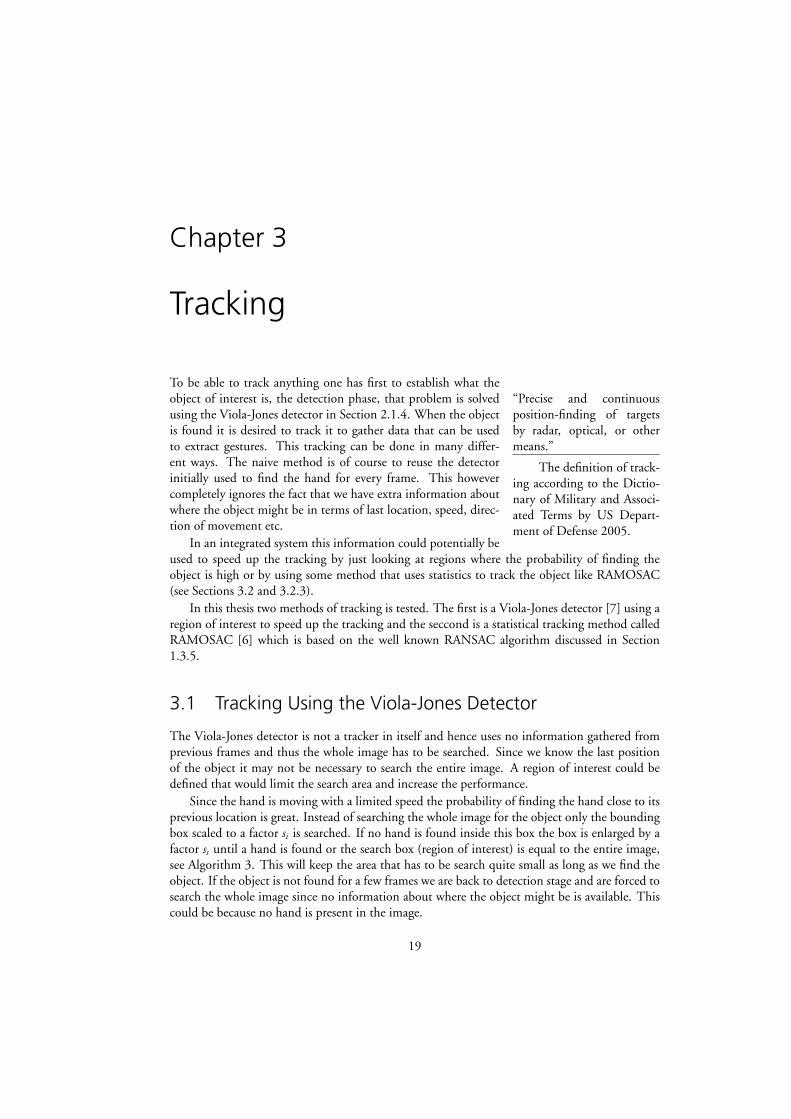
To be able to track anything one has first to establish what theobject of interest is, the detection phase, that problem is solvedusing the Viola-Jones detector in Section 2.1.4. When the objectis found it is desired to track it to gather data that can be usedto extract gestures. This tracking can be done in many differ-ent ways. The naive method is of course to reuse the detectorinitially used to find the hand for every frame. This howevercompletely ignores the fact that we have extra information aboutwhere the object might be in terms of last location, speed, direc-tion of movement etc.

In an integrated system this information could potentially beused to speed up the tracking by just looking at regions where the probability of finding theobject is high or by using some method that uses statistics to track the object like RAMOSAC(see Sections 3.2 and 3.2.3).

In this thesis two methods of tracking is tested. The first is a Viola-Jones detector [7] using aregion of interest to speed up the tracking and the seccond is a statistical tracking method calledRAMOSAC [6] which is based on the well known RANSAC algorithm discussed in Section1.3.5.

3.1 Tracking Using the Viola-Jones Detector

The Viola-Jones detector is not a tracker in itself and hence uses no information gathered fromprevious frames and thus the whole image has to be searched. Since we know the last positionof the object it may not be necessary to search the entire image. A region of interest could bedefined that would limit the search area and increase the performance.

Since the hand is moving with a limited speed the probability of finding the hand close to itsprevious location is great. Instead of searching the whole image for the object only the boundingbox scaled to a factor si is searched. If no hand is found inside this box the box is enlarged by afactor ss until a hand is found or the search box (region of interest) is equal to the entire image,see Algorithm 3. This will keep the area that has to be search quite small as long as we find theobject. If the object is not found for a few frames we are back to detection stage and are forced tosearch the whole image since no information about where the object might be is available. Thiscould be because no hand is present in the image.

19

20 CHAPTER 3. TRACKING

Input: Video framesOutput: Object bounding box

si ⇐ 0.9 {Scale down image by this factor.}ss ⇐ 1.5 {Scale up the object bounding box by this factor.}sf ⇐ 1.5 {Scale up the roi by this factor when tracking failed.}roi ⇐ size of first frameforeach frame f do

fgray ⇐ Cut out roi from f and convert to grayscale.fsmall ⇐ Scale fgray by si.fnorm ⇐ Histogram normalize fsmall .obj ⇐ Run Viola-Jones detector on fnorm

if obj found thenroi ⇐ obj bounding box scaled with a factor ssDo something usefull with the found object.

elseroi ⇐ roi scaled with a factor sf

endend

Algorithm 3: Viola-Jones tracker using roi

3.1.1 Results

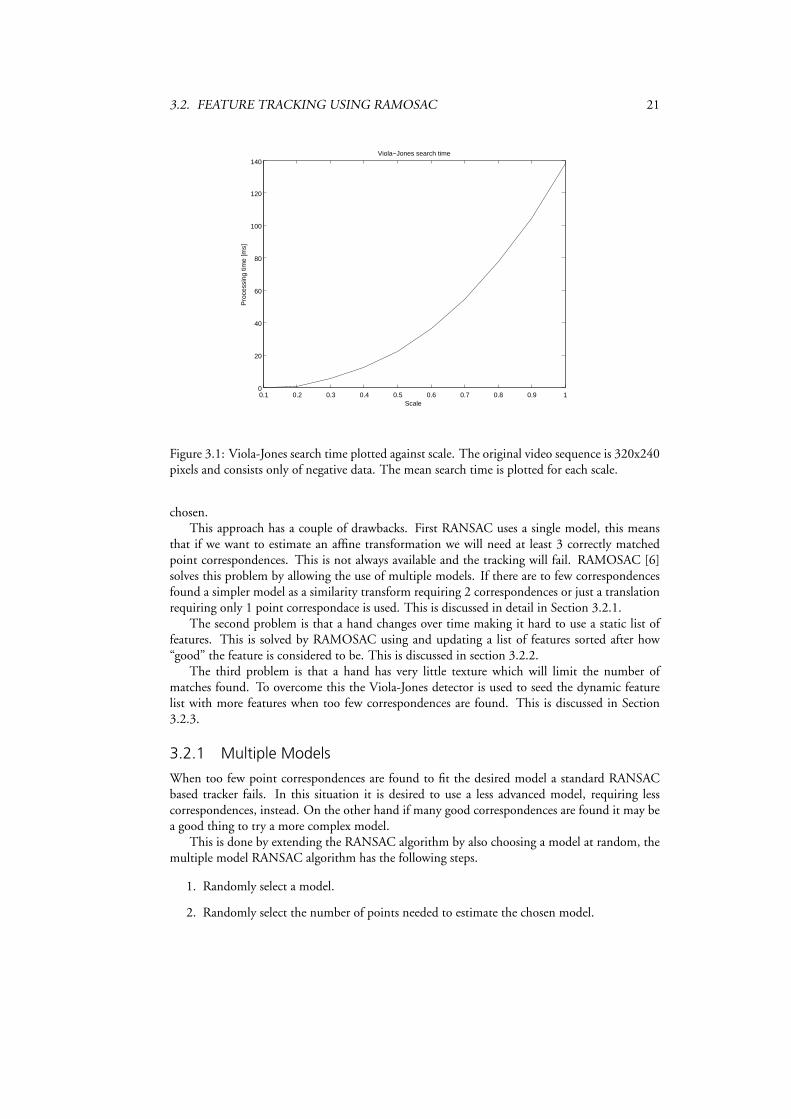
By using the method explained in Section 3.1 and just searching in a region around where thelast hand was found the time to search is somewhere around 10-20 ms/frame as long as we findthe hand, this is of course dependent on how far from the camera the hand is located that is howmuch of the image the hand occupies. If no hand is found either because the tracking failed orthere are no hands to be found the whole image has to be searched. This takes about 140mscalculated at a 320 x 240 pixel large image with no scaling that is si = 1. In most situations thisis no problem since framedropping can be used to keep the processing time down.

Interesting is that by using this method a performance gain is noticed when setting si = 1since this makes it easier to detect the hand and then also helps reduce the search area. Thishowever makes the algorithm run slower when no hand is present. This scaling factor could beused as a variable and depend on the area that is going to be searched and in this way reduce theprocessing time even more. This since a performace boost from 140ms to 100ms is noticed whensearching the whole image when si = 0.9 i.e. a area that is 19% smaller. See figure 3.1.

The actual performance of this tracker is comparable to how good the Viola-Jones cascade istrained and some tests can be found in Section 2.1.5.

3.2 Feature Tracking Using RAMOSAC

The object that is to be tracked is represented by a list of features {f1, f2, ...fn}, a feature consistsof a position and a SURF feature descriptor f = {d , x}. For every new frame the SURF featuresis calculated and matched against this list using some distance function. Those point correspon-dences are then used to estimate a transform T . The problem is now to find an estimate of Tgiven those correspondences.

RANSAC can be used for this purpose by randomly choosing the number of correspon-dences needed to estimate the desired transform, estimating the transform, evaluate the numberof consensus points and repeat n times. The transform with the most consensus points is then

3.2. FEATURE TRACKING USING RAMOSAC 21

0.1 0.2 0.3 0.4 0.5 0.6 0.7 0.8 0.9 10

20

40

60

80

100

120

140

Scale

Pro

cess

ing

time

[ms]

Viola−Jones search time

Figure 3.1: Viola-Jones search time plotted against scale. The original video sequence is 320x240pixels and consists only of negative data. The mean search time is plotted for each scale.

chosen.This approach has a couple of drawbacks. First RANSAC uses a single model, this means

that if we want to estimate an affine transformation we will need at least 3 correctly matchedpoint correspondences. This is not always available and the tracking will fail. RAMOSAC [6]solves this problem by allowing the use of multiple models. If there are to few correspondencesfound a simpler model as a similarity transform requiring 2 correspondences or just a translationrequiring only 1 point correspondace is used. This is discussed in detail in Section 3.2.1.

The second problem is that a hand changes over time making it hard to use a static list offeatures. This is solved by RAMOSAC using and updating a list of features sorted after how“good” the feature is considered to be. This is discussed in section 3.2.2.

The third problem is that a hand has very little texture which will limit the number ofmatches found. To overcome this the Viola-Jones detector is used to seed the dynamic featurelist with more features when too few correspondences are found. This is discussed in Section3.2.3.

3.2.1 Multiple Models

When too few point correspondences are found to fit the desired model a standard RANSACbased tracker fails. In this situation it is desired to use a less advanced model, requiring lesscorrespondences, instead. On the other hand if many good correspondences are found it may bea good thing to try a more complex model.

This is done by extending the RANSAC algorithm by also choosing a model at random, themultiple model RANSAC algorithm has the following steps.

1. Randomly select a model.

2. Randomly select the number of points needed to estimate the chosen model.


3. Estimate model.

4. Evaluate the model.

5. Repeat from step 1.

6. Choose the model with highest score.

The evaluation step also has to be changed to take into consideration how good the estimatedtransform is and to favor a more complex model to avoid tracking degradation.

The evaluation score is then changed from only including the number of consensus point to

S = c + log10(P(T )) + εnmin

where c is the number of consensus points, P(T ) is the probability ,nmin is the number ofpoints needed to estimate the model and ε is a scaling factor suggested to be ε = 0.1.

The probability P(T ) is calculated as

P(T ) = exp

(−λ

n∑k=1

||pt−1k − T (pt−1

k )||

)

where ptk is the polygon describing the boundary of the tracked object at time t and λ is weighted

mean

1λt

= δ1λt−1

+ (1− δ)x (3.1)

here δ is a parameter in the interval [0, 1] affecting how fast the mean changes over time.This probability will make sure that if a transform that moves the object far from the previous

location is going to be accepted it must have a large number of consensuspoints supporting it.This is in line with common sense, the object is expected to be found close to its previouslocation.

In this thesis three models/transforms are used and tested.

1. Translation transform, requiring only one point correspondence.

2. Similarity transform, requiring two point correspondences.

3. Affine transform, requiring three point correspondences.

The projective transform is not used since it requires to solve a non-linear problem makingit expensive. Furthermore this transform is not expected to give better results due to nature ofthe object being tracked and the extra information that could be calculated is not helpfull whenextracting the gestures. Even affine transformations are in most cases not needed.

3.2.2 Dynamic Feature List

Since many objects will deform or rotate over time a static list of features that describe theobject could be outdated and useless after a while. To overcome this problem RAMOSAC uses adynamic list of features that is updated with features considered “good”. This is done by keepinga list with features sorted after a score. Only the features with highest score is then used fortracking.


The score is updated as

St =

St−1 + 2 if matched, consensus pointSt−1 − 1 if matched, outlierSt−1 if not matched

which will make sure that features that often are matched and frequently used quickly will rise tothe top of the list while features that are considered to be outliers will sink to the bottom.

As the tracking goes on this list will grow. Since it is unlikely that features at the bottom ofthis list is going to give a good match only the N top entries will be tested and the bottom entriescan be thrown away to save memory and computation time.

Features found inside the boundary of the object after the estimated transformation is appliedis considered to be a part of the object and hence added to the list with a score corresponding tothe median of all scores allready in the list. This will guarantee that it is used but will not pushdown allready known good features.

3.2.3 Feature Feeding Using Viola-Jones

The benefit of using the RAMOSAC tracker to track hands is that it can be used to track anypose. The big issue is however that the performace on non textured objects is poor and it is thisproblem which we will try to solve in this section.

The idea is to use Viola-Jones detector to feed the RAMOSAC algorithm with features. Toavoid a performace hit by having to run both of the algorithms in parallel it is desired to knowwhen RAMOSAC is about to fail.

Fortunately every transform estimated also has a score connected to it. This score contains,as described in Section 3.2.1, the number of consensus points the probability and a small factorfavoring a more complex model. This score is a measure on how good the estimation is in otherwords a measure that can be used to detect when the algorithm is about to fail or is failing.

When this condition is detected the Viola-Jones detector can be used to again find the handand feed the interesting features to the dynamic feature list with a feature score equal to themedian of all features allready in the list, this is described in pseudocode in Algorithm 6.

3.2.4 Results

The great thing about the RAMOSAC algorithm is that it requires no trainingdata and is ableto track objects that changes slowly over time. An example image serie is presented in Figure3.2 where a magazine is tracked with almost 100% accuracy using a c++ implementation of thealgorithm with parameters sugested in [6].

Unfortunatelly a hand has less texture than the magazine making it harder to track reliablyusing this method. Especially the open hand pose is extra hard to track because it is not solidand features from the background will be included in the feture list. This is the reason why acombined RAMOSAC and Viola-Jones tracker was tried. This could as oposed to the Viola-Jones tracker potentialy allow the hand to sligtly transform and rotate during tracking and in thisway make the solution more robust. For comparison to the well textured object the unmodifiedRAMOSAC tracker is used to track a closed hand in Figure 3.3 and a open hand in Figure 3.4.

The combined tracker where features is extracted from regions where the Viola-Jones detectorfind the hand and fed to the RAMOSAC feature list turned out not to work very well. The mainissue is that the hand has to little texture resulting in to few features found belonging to the handand too many features belonging to the background. This made the tracking fail quite fast sincethe feature list got polluted with false positive features.


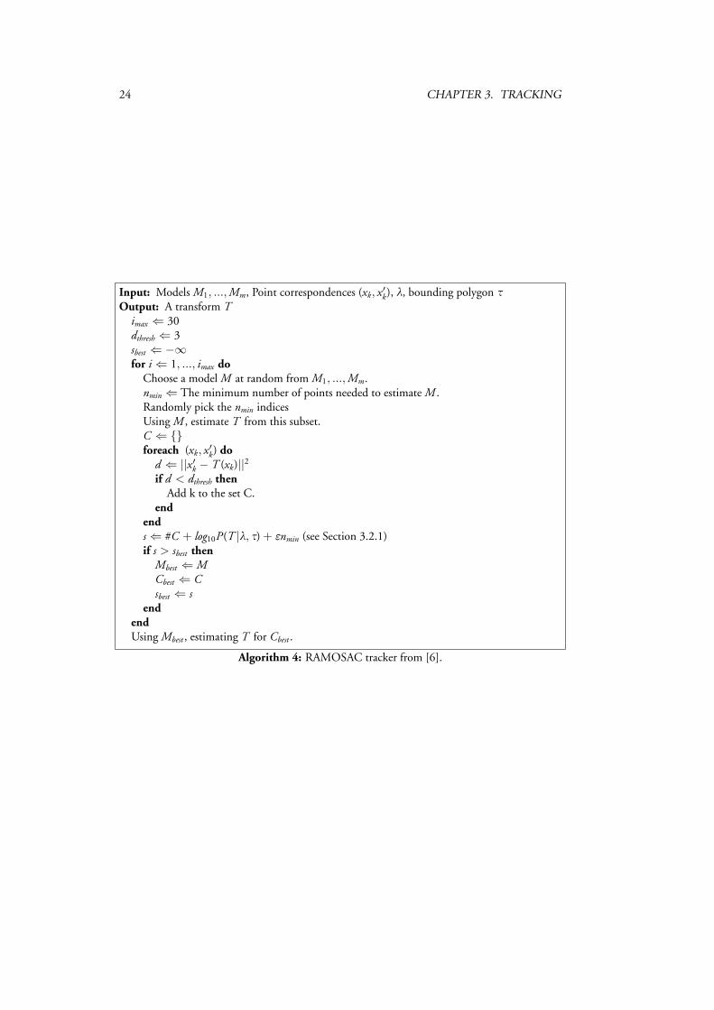
Input: Models M1, ..., Mm, Point correspondences (xk, x′k), λ, bounding polygon τOutput: A transform T

imax ⇐ 30dthresh ⇐ 3sbest ⇐ −∞for i ⇐ 1, ..., imax do

Choose a model M at random from M1, ..., Mm.nmin ⇐ The minimum number of points needed to estimate M .Randomly pick the nmin indicesUsing M , estimate T from this subset.C ⇐ {}foreach (xk, x′k) do

d ⇐ ||x′k − T (xk)||2if d < dthresh then

Add k to the set C.end

ends ⇐ #C + log10P(T |λ, τ) + εnmin (see Section 3.2.1)if s > sbest then

Mbest ⇐ MCbest ⇐ Csbest ⇐ s

endendUsing Mbest , estimating T for Cbest .

Algorithm 4: RAMOSAC tracker from [6].


Input: Video frames, Initial bounding polygon τOutput: Location of object in each frame

m⇐ 100 {Number of features to store.}Calculate features Pframe in te first video frame.Pobj ⇐ {p ∈ Pframe}Sp ⇐ 0 for all p ∈ Pobj

foreach frame f doUpdate λ according to Equation 3.1.Calculate features Pframe in f .Sort Pobj with respect to S.Ptop ⇐ {first m features in Pobj }Find matches M between Ptop and Pframe.Estimate transform T according to Table 4.τ⇐ T (τ)foreach p ∈ Pobj do

Sp =

Sp + 2 if matched, consensus point (p ∈ M , p ∈ C )Sp − 1 if matched, outlier (p ∈ M , p /∈ C )Sp if not matched (p /∈ M )

endif #(I ) > 4 and P(T |λ, τ) > 0.1 then

Pnew ⇐ {p ∈ Pframe|p inside τ} \ Msnew ⇐ median{Sp}p∈Ptop

Pobj ⇐ Pobj ∪ Pnew

SP ⇐ snew for every p ∈ Pnew

endend

Algorithm 5: RAMOSAC tracker with dynamic feature list from [6].


Input: Video frames, Initial bounding polygon τOutput: Location of object in each frame

s ⇐ 1.5 {Score threshold}foreach frame f do{τ, Ts} ⇐ RAMOSAC (f , τ) {Run RAMOSAC tracker as described in Tables 4 and 5. Ts isthe transform score. }if Ts < s then

obj ⇐ Run Viola-Jones detector on frameif obj found then

Pvj ⇐ Extract SURF features from the found region.Find matches M between Pvj and Pobj see Table 5.foreach p ∈ Pvj do

Sp ={

Sp + 2 if matched, consensus point (p ∈ M )Sp if not matched (p /∈ M )

endPnew ⇐ {p ∈ Pvj} \Msnew ⇐ median{Sp}p∈Pobj

Pobj ⇐ Pobj ∪ Pnew

SP ⇐ snew for every p ∈ Pnew

endend

end

Algorithm 6: RAMOSAC tracker with feature feeding.

An idea to make it work better is to use a skin color detector to determine if the featureactually belongs to the hand, this is however not tested.


100

200

300

400

500

600

700

800

900

Figure 3.2: Plain RAMOSAC without feature feeding, tracking magazine with almost 100%accuracy.

100

200

300

400

500

600

700

800

900

Figure 3.3: Plain RAMOSAC without feature feeding, tracking closed hand.


100

200

300

400

500

600

700

800

900

Figure 3.4: Plain RAMOSAC without feature feeding, tracking opened hand. As can be seenfeatures from the background makes it fail.

Chapter 4

Gesture

“Words represent your intel-lect.The sound, gesture andmovement represent yourfeelings.”

Patricia Fripp

In this chapter we will discuss the method used to classify ges-tures. The matching of gestures is a form of pattern matchingwhich is a well researched area [17, 18, 19]. Matching patterns isa wide area covering problems ranging from simple ones as to seeif two random variables are the same to matching multidimen-sional data.

For our work we need to be able to determine if a gestureperformed is likely to be one of the predefined templates. Weexpect the input data to be a series of points sampled from thetrajectory described by a hand.

4.1 Comparing Different Gestures

The main difficulties in comparing different gestures in this thesis are the following.

• Compare trajectories independent of where the trajectories start.

• Measure differences between trajectories.

• Compare trajectories with different number of data points.

• Different users performing the same gesture in different time.

The first problem is perhaps the easiest to circumvent by transforming the attained data in aclever way.

To motivate why this is a problem for our application consider the case where one userperforms a certain gesture two times, once starting from point (x0, y0) and the other one identicalbut starting at point (x0 + δ, y0), this would generate a difference in the measure, the differencebetween the to identical gestures performed at different locations are,

d =n∑

j=0

√(xj + δ− xj)2 − (yj − yj)2 = nδ.

This error will propagate through all kinds of template matching and thus we have to reduce theeffect.

29

30 CHAPTER 4. GESTURE

This said, it still may be the part where one has to try different methods and use the one thatperforms well for the current application. The transform we used is the one described in Section1.3.3 which fullfills our requirments.

By transforming our coordinates to the angular space, T : (x, y) → a, a ∈ [0, 360] wereduced the two dimensional data to one dimension which in turn will be matched against a setof predefined templates. Further on the transformed data was quantized in steps of 360

255 resultingin 255 different values which fits nice into 8-bit data types. This transformation and quantizationmakes it easier to match data because one dimensional data is easier to match and fit.

4.2 Matching

A rough description of matching algorithms is to find a distance function, d (S, T ), which can beapplied to a signal, S and a template, T , where

S = {si}Lsi=0

T = {ti}Lti=0.

We need our distance function to have certain properties:

d (S, T ) > 0

d (S, T ) = 0⇐ S = T

d (S, T ) = d (T , S).

These criteria are similar to the ones for distance functions on metric spaces however we lack thetriangle inequality and the property d (s, t) = 0⇒ s = t.

If one can find such a function one can easily implement a nearest neighbor algorithm whereone calculates the distance between the signal and all the possible templates. The simplest dis-tance function would be the squared Euclidean distance

d (S, T ) =n∑

i=0

(si − ti)2,

where n is the signal length. This requires that both signals have the same length. Due to thequantization the maximum distance is

n∑i=0

(255− 0)2 = n2552.

With this value we can make a rough estimate of how well a signal fits a template. Since theerrors will be in the range [0, n2552] we can scale d (S, T ) by dividing with n2552 to get a valuebetween 0 and 1, this scaling is used in the paper. When implementing the algorithm on caninstead scale by dividing with just n to get the error in the range [0, 2552] this might be a bitfaster.

4.3 Different Signal Length

A frequent problem is that without any preprocessing of the data the length of the signal rarelymatches the length of the template. It is easy to normalize the length of the templates since theyare predetermined but how do one adjust the signal length without distorting the signal? Thetwo easiest solutions are to either pad one signal or remove data from the other signal.

4.3. DIFFERENT SIGNAL LENGTH 31

4.3.1 Cut-Off

If data is removed from the signal that is longer the result would have been

d (s, t) =min(Ls,Lt )∑

i=0

(si − ti)2.

with the quantization the maximum error is

min(Ls,Lt )∑i=0

(255− 0)2 = min(Ls, Lt )2552.

This solution is not good since a signal of length 1 will have a maximum distance of 255 and willnot cover the variety of the signal.

4.3.2 Padding

If we pad a signal, that is if Ls < Lt the sequence s is padded with zeros in the end to match thesignal length. Analog if Lt < Ls.

d (s, t) =max(Ls,Lt )∑

i=0

(si − ti)2.

Because of the quantization the maximum distance is

max(Ls,Lt )∑i=0

(255− 0)2 = max(Ls, Lt )2552.

This method might be better for some signals but it still is not good.

4.3.3 Dynamic Time Warping (DTW)

DTW is a nonlinear mapping which solves the problem with different signal lengths and theproblem with users performing the same gesture in different time. DTW tries to “describe” thesecond signal with the first by finding the data in one signal that matches the second signal bestrestricted by some rules. What we try to do is warp the indices of the signals so that we let thedata in one signal at index i describe the data in the other signal at indices jk, thus we allow onedata point to be able to describe the behaviour at multiple points.

If we denote the samples from the signal by Si and the samples from the template by Ti weconstruct the matrix

C =

d (S1, T1) d (S1, T2) . . . d (S1, Tm)d (S2, T1) d (S2, T2) . . . d (S2, Tm)...

. . ....

d (Sn, T1) d (Sn, T2) . . . d (Sn, Tm)

,

where d (x, y) is a distance function, most commonly the Euclidean distance. The goal now is tofind a path through this matrix with minimal cost. We also require that the path starts in C1,1

and ends in Cn,m (boundary conditions). The path must also be continuous and monotonical,by this we require each step to either be to the right, down, or diagonally down to the right.


This can be implemented using dynamic programming by starting at C1,1 moving one stepat a time, taking the step that has the least cost, and then update the cost-matrix and continueuntil we reach Cn,m.

If two identical signals, S and T , are matched using DTW the following holds

i = j ⇒ d (Si, Tj) = 0,

which results in the main diagonal of the cost matrix only consist of zeros,

C =

0 d (S1, T2) . . . d (S1, Tm)d (S2, T1) 0 . . . d (S2, Tm)...

. . ....

d (Sn, T1) d (Sn, T2) . . . 0

,

and therfor DTW can map each index i to itself resulting in a total distance of 0 which was oneof the requirements.

In [9] a method called Derivative Dynamic Time Warping, DDTW, was introduced. Thismethod was introduced to reduce the ammount of warping, reducing singularities in the match-ing. The idea is to use the derivative of the signal in DTW instead of the original signal. Thisway an additional rule is added namely that local extremas should be matched to other localextremas. We refer to the cited paper for more information. Since this method only added theneed of taking the derivative of the signal before matching we added the method to the completesystem.

4.4 Tests and Results

To illustrate the three methods we tested with three artificial made examples and then two realworld samples captured from a regular mouse. In the artificial examples we made one templateand one signal to match against the template. The signal corresponds to the template downsam-pled with a factor of two and with added noise. All errors were computed as

Error =1

2552L

L∑i=0

|Ti − Si|2, (4.1)

where T denotes the template and S the signal. The division by 2552L asserts that the error is inthe range [0, 1] for easy comparison.

The first example in Figure 4.1 illustrates the fact that the Padding method will in fact workwell when signals are close to zero in the end. The second example is a strictly increasing function,t4, which shows that the Padding method works poorly see Figure 4.2. In Figure 4.3 we havethe last example which is closest to a real world example. We see that both the Padding and theCut-Off method fails whereas the DTW method works very well, as in the other two examples.

The real world samples were constructed by first specifying templates mathematically. Wehave a clock-wise circle and a clock-wise triangle template. By recording mouse movement wegot two samples per template. We tried to make one of the samples shorter than the templatelength and the other longer. Since the results from Figures 4.1, 4.2 and 4.3 lead to the conclusionthat DTW in fact works much better than trivial methods the following tests just displays theDTW method. We tested to do each gesture two times with a mouseand the results can be seenin Figures 4.4 and 4.5.

4.4. TESTS AND RESULTS 33

0 0.5 1 1.5 2 2.5 3 3.50

2

4

6

8

10

12

Time

data

Cut−Off method − Error: 9.0046

TemplateSignal

0 0.5 1 1.5 2 2.5 3 3.50

2

4

6

8

10

12

Time

data

Zero−Pad method − Error: 4.5491

TemplateSignal

0 0.5 1 1.5 2 2.5 30

2

4

6

8

10

12Pairing done by DTW

Time

data

0 0.5 1 1.5 2 2.5 3 3.50

2

4

6

8

10

12

Time

data

DTW method − Error: 0.0010

TemplateSignal

Figure 4.1: The decaying function e−t2and its downsampled version with noise and the com-

parison. Cut-Off method (upper left), padding (upper right) and DTW (lower right).

The first test was the clockwise circle which can be found in Figure 4.4. One thing ofimportance is to notice that the signals are quite noisy, this requires some attention by filteringthem.

The second gesture to be tested was the clockwise triangle in Figure 4.5. The interesting parthere is that the template only consist of three different angles corresponding to the slopes of thetriangle. This makes it hard for DTW to match since it is likely that DTW can describe theseangles with data from almost any signal since the signals contains noise which most likely willcover these angles.

Signal Triangle template Circle templateTriangle template 0 0.0104Triangle 1 0.0069 0.0084Triangle 2 0.0046 0.0060Circle template 0.0104 0Circle 1 0.0167 0.0032Circle 2 0.0184 0.0094

Table 4.1: Signal VS Template errors.

In Table 4.1 we tested each of the signals and templates against the templates to find outif a correct match would be done. We used the same signals as in Figures 4.1 4.2 and 4.3but filtered them using a moving average filter of length 4. The bold figures are the lowest andthe result is that DTW manages to match the signals correct. A confirmation that the distancebetween two identical signals is 0 using DTW where also achieved.


0 0.5 1 1.5 2 2.5 3 3.50

20

40

60

80

100

Time

data


TemplateSignal

0 0.5 1 1.5 2 2.5 3 3.50

20

40

60

80

100

Time

data


TemplateSignal

0 0.5 1 1.5 2 2.5 30

20

40

60

80

100Pairing done by DTW

Time

data

0 0.5 1 1.5 2 2.5 3 3.50

20

40

60

80

100

Time

data


TemplateSignal

Figure 4.2: The increasing function t4 and its downsampled version with noise and the compar-ison. Cut-Off method (upper left), padding (upper right) and DTW (lower right).

0 0.5 1 1.5 2 2.5 3 3.5−1

−0.5

0

0.5

1

1.5

Time

data


TemplateSignal

0 0.5 1 1.5 2 2.5 3 3.5−1

−0.5

0

0.5

1

1.5

Time

data


TemplateSignal

0 0.5 1 1.5 2 2.5 3−1

−0.5

0

0.5

1

1.5Pairing done by DTW

Time

data

0 0.5 1 1.5 2 2.5 3 3.5−1

−0.5

0

0.5

1

1.5

Time

data


TemplateSignal

Figure 4.3: The function cos(t) and its downsampled version with noise and the comparison.Cut-Off method (upper left), padding (upper right) and DTW (lower right).

4.4. TESTS AND RESULTS 35

−50 0 50

0

20

40

60

80

Circle template and signals

0 100 200 3000

100

200

300Angular space representation

0 50 100 1500

100

200

300Short signal match, error: 0.0032

0 100 200 300 4000

100

200

300Long signal match, error: 0.0094

Figure 4.4: Circle template and signals.

0 50 100

0

20

40

60

80

Triangle template and signals

0 100 200 3000

100

200

300Angular space representation

0 50 1000

100

200

300Short signal match, error: 0.0069

0 100 200 3000

100

200

300Long signal match, error: 0.0093

Figure 4.5: Triangle template and signals.

Chapter 5

Complete System

“A project is complete whenit starts working for you,rather than you working forit.”

Scott Allen

With all the methods and algorithms discussed in the previ-ous chapters we can now find, track and match the movementsagainst templates. In this chapter we will discuss the glue betweenthem and how to make a complete system capable of emulating amouse as well as classify performed gestures. Before we give anydetails about the complete system we will list some backgrounddetails.

5.1 Background Facts and Considerations

Since we would like this to run on a mobile platform the only “good” choices for programminglanguage was C or perhaps C++, we decided to use C++. To get started quickly we also decidedon using OpenCV and Boost. OpenCV [12] is an open source library for Computer Visionalgorithms. This is a large package of functions and data structures often used. At the timeof writing OpenCV was a “mess”, no clear structure and we would like to wish for a moreobject oriented approach (which currently is under development). Even though there are somedrawbacks design-wisely using OpenCV it felt like a good choice since Nokia has adopted someof the ideas behind OpenCV and started their NokiaCV [20] library. We also used the Boostlibrary [11] which is a huge c++ library with many good implementations of data structures andalgorithms.

Instead of writing our own user interface, we had the great opportunity to work with aframework called Cascades which is developed by TAT [21] (The Astonishing Tribe). This waywe did not have to worry about that part at all. Cascades is an advanced engine, parsing XML-like files which describes the entire user interface, graphics, effects, user input, etc. Cascadeshandles all the input to a device and has native support for touch screens. Our approach was toemulate a touch screen using our system for hand tracking and the performed gestures can easilybe sent as events for Cascades to handle. This way it is very easy to incorporate our system in anyCascades application.

The targeted hardware was the Beagle Board (see Figure 5.1) but as time got short we had toskip the implmentation on this devices. For comparacens to the computer we used for develop-ment and testing see Table 5.1 wher some of the specifications are listed.

37

38 CHAPTER 5. COMPLETE SYSTEM

Processor Texas Instruments OMAP3530 at 600Mhzapprox. laptop performanceover 1200 Dhrystone MIPS256kB L2 cache at 600MHz

DSP and Graphics TI TMS320C64x+ DSP, up to 430MHzSupports OpenGL ES 2.0 accelerationrendering about 10 million polygons per second

Power Powered over USB or external 5V adapterrequires about 300mA

Development Boot code store in ROMBoots from NAND memory, SD/MMC, USB, or SerialAlternative Boot source buttonRuns Linux

Table 5.1: BeagleBoard specifications

5.2 Technicalities and Implementation

In the final system we used the Viola-Jones detector to find the hand (see Section 2.1.4) andthe Viola-Jones region of interest tracker (see Section 3.1 because of better performance than theRAMOSAC algorithm 3.2.3 that was tested.

The Viola-Jones tracker/detector was using an alternating scheme to avoid searching the sameframe twice. When a pose was found the system locked to this pose until it disappeared and thealternating scheme took over again.

For the gesture recognition, the data from the tracking stage was buffered, translated intoangular space and derivated as described in Section 4. These translation, scale and rotationinvariant data series was then matched against templates using the Dynamic Time Warping al-gorithm. The results where sent as events into the user interface to be mapped to some functionlike stop, play, pause, etc.

Since we noticed the problem with noise in Section 4.4 we decided to implement a movingaverage filter (MA-filter) to smooth the obtained signal. This is done in parallell to the dataacquisition. The length of the filter has a not very suprising but interesting property. If the filteris short its easier to distinguish between circle and triangle but harder to classify a straight lineand vice versa. The filter length that gave a good compromise turned in this case out to be 3.

The templates where all 32 samples long and contained the “perfect” geometric shapes thatwas chosen for the gestures. For example a straight line is 32 zeros while a circle is 32 eights since32 ∗ 8 = 256 and hence cover the whole circle. Those templates where then processed by theMA-filter using the empirical determind length 3. This filter will do nothing for the line andcircle template but will smooth out other more complex templates such as the triangle.

We also built a mouse emulator that emulated a touchscreen. The open and closed poseswhere mapped to touch and click. This allowed the user to move the mouse cursor using anopen hand and click or drag by closing the hand.

5.3 Tests

Since this is a system and not a method its hard to give quantitative results. Instead we let fivepeople test the system and give their feedback on how they thought it worked. The tests where

5.3. TESTS 39

Figure 5.1: The BeagleBoard with its peripheral connections and some specifications (image fromhttp://beagleboard.org/hardware).

done in the same environment as the Viola-Jones tracker where trained to minimize the impactof a limited training set. The test persons tested two different system mouse emulator and gestureclassifier.

Comments we got on the mouse emulator where open hand was mapped to move and closedwas mapped to click/drag.

• The mouse cursor jumps when clicking making it hard to hit the desired click area.

This is because the open and closed hand has different sizes which will make the center-point jump when changing pose. This should not be to hard to correct by introducing anoffset that is changed as the size of the bounding box is changed. One could also save theprevious positions and use them when the pose changes.

• The system does not find my hand.

As said before the training is quite limited making the system sensitive to rotations andto variations in the form and shape of different users. A more “complete” trainingset andsome means to estimate the rotation would probably solve this problem.

• The cursor is not still even when my hand is not moving.

A problem arising from the fact that the Viola-Jones detector is not finding the exactsame bounding box in every frame when the hand is still. This effect could be reducedby filtering the signal more aggressively and perhaps using a threshold to remove smallmovements and make the user feel as if the cursor is still.

• Its exhausting to keep the hand up infront of the camera.

Yes it is, but the system is not intended to be a mouse/keyboard replacement but a com-plement when such devices is hard to use for examples presentations.

http://beagleboard.org/hardware


Comments on the gesture recognition system.

• Sometimes the system recognize one gesture as another.

There are quite a lot of noise in the signal which makes the matching unstable. More workis needed on the filtering of the signals to make it more reliable using DTW. It might be agood idea to try out other methods for matching such as artificial neural nets.

• The system does not always find my hand.

The same problem as for the mouse emulator.

• Sometimes the system detects different actions even though I do the same gesturemultiple times.

It is very hard to do the same gesture twice (almost impossible), even though the userthinks he/she is performing the same gesture there is some variation due to noise, poseand position. We also have the fact that the templates are not adapted to anyone. Morework has to be done to adapt the templates to the user instead of the user adapting to thesystem. However, the results from the system is the same for recorded video sequences.

5.4. CONCLUSIONS AND FUTURE WORK 41

5.4 Conclusions and Future Work

From this thesis answers to some of the questions have been found. We have actually imple-mented a system that works in preliminary tests. There are still some problems to solve.

There are however a number of issues that needs to be addressed to make the system ul. Firstof all a much larger and diversified training set has to be collected and the Viola-Jones detectorneeds to be retrained with this new data. This will make the system much more robust and makeit easier to extract continuous data series which in turn would lead to better performance of thegesture detector.

The way we have implemented the Dynamic Time Warping, only using the derivative of theangles, makes it hard to, for an example, distinguish a clockwise circle and a clockwise trianglesince they often cover the same angle space when drawn in the air. This could improve if onecould reduce the ammount of noise by having a more reliable tracking and better filtering.

The implementation ran very well on a standard PC without any special optimizations, usingthe Viola-Jones region of interest tracker the time to process each frame was around 10 ms as longas the hand was found. To search the entire frame takes around 100 ms but frame dropping canbe used to lover the processing needs.

Unfortunately we didn’t have time to get the system up and running on the Beagle Board.But since we obtained around 100 fps at a normal 2 GHz PC there are margins. Since mostcheap cameras can not acquire frames faster than 10-20 fps. Our tests shows that this rate isenough to run the system at a 5-10 times slower computer without any frame dropping.

Our implementation is not optimized and could probably be quite a bit faster if considera-tions where taken to avoid floating point operations in favor for integer operations. This wouldmake a big difference at low end computers like the Beagle Board without hardware acceleratedfloating point operations.

More and more mobile platforms as the Beagle Board has built in functions for vectorizationand contain digital signal processors (DPS) and graphics processing units (GPU) that potentiallycould be used to speed up the execution. This is however outside the scope of this thesis.

The simple algorithm with scaling search windows used in the Viola-Jones tracker in Section3.1 could be extended by incorporating a Kahlman filter estimating the next location and usingthis position as the center of the search window. The estimated speed could then be used toform a rectangle to search in. This could decrease the search window for the object even furtherand in this way speed up the algorithm. Further more the data from the Kahlman filter couldbe fed directly into the gesture classifier to take into account accelerations and velocities duringa gesture. This way it might be possible to get more nuance into gestures making differencebetween an “angry” circle gesture and a “calm” circle gesture.

In Section 4 we discussed the matching of gestures. Interesting future work could be toimplement an algorithm for adaptive templates where the standard templates adapt to the userinstead of the other way around. One way to do this might be to evaluate if the user is “satisfied”with the performed gesture and then weight the initial template with data from the performedgesture. This could potentially be done automatic by monitoring the users next action.

It would also be very interesting to make automatic training of different poses as the person isusing the system. The problems here are many and might be too hard to overcome. For instance,the ADA-boost training does not work incrementally. One might be able to use Learn++ orADA-boost.M1 see [22].

Other elements that need to be researched on a more user-interaction based level are amongother things.

• Where is it desired to use this kind of input?


• What gestures are logical for us human beings?

• Which poses should be trained if only a limited set can be used?

• Is there any other feature except touchpad/mouse-emulation and gesture recognition thatwould make sense?

There certainly are more topics that would be interesting to explore as stated above not onlytopics including future work for this particular system. There are answers to questions abouthuman↔device interaction that must be sought. This is of great importance now and in thefuture to make our daily interactions with different devices less cumbersome than today.

List of Figures

1.1 Color and Grayscale Conversion . . . . . . . . . . . . . . . . . . . . . . . . . 31.2 Integral Image . . . . . . . . . . . . . . . . . . . . . . . . . . . . . . . . . . 41.3 Example of samples from a gesture. The angle of the arrows represent the angular

space. . . . . . . . . . . . . . . . . . . . . . . . . . . . . . . . . . . . . . . 61.4 Resulting tranform of the samples in Figure 1.3. . . . . . . . . . . . . . . . . . 61.5 Difference of Gaussian pyramid generated from a hand. Matlab script written

by Andrea Vedaldi. . . . . . . . . . . . . . . . . . . . . . . . . . . . . . . . . 71.6 Original image. . . . . . . . . . . . . . . . . . . . . . . . . . . . . . . . . . 81.7 SIFT - features displayed. . . . . . . . . . . . . . . . . . . . . . . . . . . . . 91.8 Neighbors to the current pixel. Neighbors are marked with o’s, the current pixel

is marked with x. . . . . . . . . . . . . . . . . . . . . . . . . . . . . . . . . . 91.9 Discretization of Gaussian used by SURF features. Image from [15]. . . . . . . 101.10 Line fitting, Least-Square compared to RANSAC. . . . . . . . . . . . . . . . . 101.11 Line fitting, Least-Square compared to RANSAC with many outliers present.

Circles are inliers and stars are outliers. . . . . . . . . . . . . . . . . . . . . . 10

2.1 A cascade with three features. If one fail we are done. . . . . . . . . . . . . . . 112.2 Viola-Jones features. The pixelsum of the white areas are subtracted from the

pixelsum of the black areas. . . . . . . . . . . . . . . . . . . . . . . . . . . . 122.3 Examples from the training set for the open hand pose. . . . . . . . . . . . . . 132.4 Examples from the training set for the closed hand pose. . . . . . . . . . . . . 142.5 The poses used, closed pose to the left and open pose to the right. . . . . . . . . 172.6 Test movie A, Viola-Jones detector. . . . . . . . . . . . . . . . . . . . . . . . 172.7 Test movie B, Viola-Jones detector. . . . . . . . . . . . . . . . . . . . . . . . 18

3.1 Viola-Jones search time plotted against scale. The original video sequence is320x240 pixels and consists only of negative data. The mean search time isplotted for each scale. . . . . . . . . . . . . . . . . . . . . . . . . . . . . . . 21

3.2 Plain RAMOSAC without feature feeding, tracking magazine with almost 100%accuracy. . . . . . . . . . . . . . . . . . . . . . . . . . . . . . . . . . . . . . 27

3.3 Plain RAMOSAC without feature feeding, tracking closed hand. . . . . . . . . 273.4 Plain RAMOSAC without feature feeding, tracking opened hand. As can be

seen features from the background makes it fail. . . . . . . . . . . . . . . . . . 28

4.1 The decaying function e−t2and its downsampled version with noise and the

comparison. Cut-Off method (upper left), padding (upper right) and DTW(lower right). . . . . . . . . . . . . . . . . . . . . . . . . . . . . . . . . . . . 33

43

44 LIST OF FIGURES

4.2 The increasing function t4 and its downsampled version with noise and thecomparison. Cut-Off method (upper left), padding (upper right) and DTW(lower right). . . . . . . . . . . . . . . . . . . . . . . . . . . . . . . . . . . . 34

4.3 The function cos(t) and its downsampled version with noise and the compar-ison. Cut-Off method (upper left), padding (upper right) and DTW (lowerright). . . . . . . . . . . . . . . . . . . . . . . . . . . . . . . . . . . . . . . 34

4.4 Circle template and signals. . . . . . . . . . . . . . . . . . . . . . . . . . . . 354.5 Triangle template and signals. . . . . . . . . . . . . . . . . . . . . . . . . . . 35

5.1 The BeagleBoard with its peripheral connections and some specifications (imagefrom http://beagleboard.org/hardware). . . . . . . . . . . . . . . . . 39

http://beagleboard.org/hardware

List of Tables

2.1 Viola-Jones performance on test movies A and B. Examples from the movies canbe seen in Figures 2.6 and 2.7. . . . . . . . . . . . . . . . . . . . . . . . . . . 15

4.1 Signal VS Template errors. . . . . . . . . . . . . . . . . . . . . . . . . . . . . 33

5.1 BeagleBoard specifications . . . . . . . . . . . . . . . . . . . . . . . . . . . . 38

45

46 LIST OF TABLES

List of Algorithms

1 The Ada boost algorithm. . . . . . . . . . . . . . . . . . . . . . . . . . . . . 152 The algorithm to build a cascade detector as proposed by [7]. . . . . . . . . . . 163 Viola-Jones tracker using roi . . . . . . . . . . . . . . . . . . . . . . . . . . . 204 RAMOSAC tracker from [6]. . . . . . . . . . . . . . . . . . . . . . . . . . . 245 RAMOSAC tracker with dynamic feature list from [6]. . . . . . . . . . . . . . 256 RAMOSAC tracker with feature feeding. . . . . . . . . . . . . . . . . . . . . 26

47

48 LIST OF ALGORITHMS

Bibliography

[1] GestureTek, “Gesturetek website,” 2009. http://www.gesturetek.com.

[2] M. Kölsch, M. Turk, T. Höllerer, and J. Chainey, “Handvu website,” 2004. http://www.movesinstitute.org/~kolsch/HandVu/HandVu.html.

[3] M. Kolsch and M. Turk, “Fast 2d hand tracking with flocks of features and multi-cueintegration,” pp. 158–158, June 2004.

[4] M. Kölsch and M. Turk, “Robust hand detection,” in In International Conference on Auto-matic Face and Gesture Recognition (to appear), Seoul, Korea, pp. 614–619, 2004.

[5] M. Kölsch, M. Turk, T. Höllerer, and J. Chainey, “Vision-based interfaces for mobility,” inIn Intl. Conference on Mobile and Ubiquitous Systems (MobiQuitous, 2004.

[6] P. Strandmark, “Feature tracking with multiple models,” 2008.

[7] P. Viola and M. Jones, “Rapid object detection using a boosted cascade of simple fea-tures,” in Proc. Conf. Computer Vision and Pattern Recognition, IEEE Computer SocietyPress, 2001.

[8] Y. Freund and R. E. Schapire, “A short introduction to boosting,” 1999.

[9] E. J. Keogh and M. J. Pazzani, “Derivative dynamic time warping,” in In First SIAM Inter-national Conference on Data Mining (SDM’2001, 2001.

[10] F. Dadgostar and A. Sarrafzadeh, “Gesture recognition through angle space.”

[11] Boost, “Boost website,” 2009. http://www.boost.org/.

[12] “Opencv website,” 2009. http://opencv.org/.

[13] C. Harris and M. Stephens, “A combined corner and edge detection,” in Proceedings of TheFourth Alvey Vision Conference, pp. 147–151, 1988.

[14] D. G. Lowe, “Distinctive image features from scale-invariant keypoints,” International Jour-nal of Computer Vision, vol. 60, pp. 91–110, 2004.

[15] H. Bay, A. Ess, T. Tuytelaars, and L. van Gool, “Speeded-up robust features (surf ),” Com-puter Vision and Image Understanding (CVIU), vol. 110, pp. 346–359, June 2008.

[16] R. Lienhart and J. Maydt, “An extended set of haar-like features for rapid object detection,”in IEEE ICIP 2002, pp. 900–903, 2002.

49

http://www.gesturetek.com

http://www.movesinstitute.org/~kolsch/HandVu/HandVu.html

http://www.movesinstitute.org/~kolsch/HandVu/HandVu.html

http://www.boost.org/

http://opencv.org/

50 BIBLIOGRAPHY

[17] P. Hong, M. Turk, and T. S. Huang, “Constructing finite state machines for fast gesturerecognition,” in Pattern Recognition, 2000. Proceedings. 15th International Conference on,vol. 3, pp. 691–694 vol.3, 2000.

[18] B. Signer, U. Kurmann, and M. C. Norrie, “igesture: A general gesture recognition frame-work,” in Document Analysis and Recognition, 2007. ICDAR 2007. Ninth International Con-ference on, vol. 2, pp. 954–958, 2007.

[19] Y. Wu and T. S. Huang, “Vision-based gesture recognition: A review,” Lecture Notes inComputer Science, vol. 1739, 1999.

[20] “Nokiacv website,” 2009. http://research.nokia.com/research/projects/nokiacv/.

[21] “The astonishing tribe website,” 2009. http://www.tat.se/.

[22] M. M. Hussein Syed Mohammed, James Leander and R. Polikar, “Can adaboost.m1learn incrementally? a comparison to learn++ under different combination rules,”vol. 4131/2006, pp. 254–263, September 2006.

http://research.nokia.com/research/projects/nokiacv/

http://research.nokia.com/research/projects/nokiacv/

http://www.tat.se/

Master’s Theses in Mathematical Sciences 2009:E14ISSN 1404-6342

LUTFNA-3179-2009

MathematicsCentre for Mathematical Sciences

Lund UniversityBox 118, SE-221 00 Lund, Sweden

http://www.maths.lth.se/

a system for real time gesture recognition · a system for real time gesture recognition daniel...

Documents