HAL Id: inria-00602327https://hal.inria.fr/inria-00602327

Submitted on 22 Jun 2011

HAL is a multi-disciplinary open accessarchive for the deposit and dissemination of sci-entific research documents, whether they are pub-lished or not. The documents may come fromteaching and research institutions in France orabroad, or from public or private research centers.

L’archive ouverte pluridisciplinaire HAL, estdestinée au dépôt et à la diffusion de documentsscientifiques de niveau recherche, publiés ou non,émanant des établissements d’enseignement et derecherche français ou étrangers, des laboratoirespublics ou privés.

A switched system approach to exponential stabilizationthrough communication network

Alexandre Kruszewski, Wenjuan Jiang, Emilia Fridman, Jean-Pierre Richard,Armand Toguyeni

To cite this version:Alexandre Kruszewski, Wenjuan Jiang, Emilia Fridman, Jean-Pierre Richard, Armand Toguyeni. Aswitched system approach to exponential stabilization through communication network. IEEE Trans-actions on Control Systems Technology, Institute of Electrical and Electronics Engineers, 2012, 20(4), pp.887-900. �10.1109/TCST.2011.2159793�. �inria-00602327�

1

A Switched System Approach to Exponential

Stabilization through Communication Network

A. Kruszewski, W.-J. Jiang, E. Fridman, J.-P. Richard, A. Toguyeni

Abstract

The present paper considers a networked control loop, wherethe plant is a “slave” part, and the

remote controller and observer constitute the “master”. Since the performance of Networked Control

Systems (NCS) depends on the Quality of Service (QoS) available from the network, it is worth to

design a controller that takes into account qualitative information on the QoS in realtime. The goal of

the design is to provide a controller that guarantees two things: 1) high performances (here expressed

by exponential decay rates) when the QoS remains globally the same; 2) global stability when the

QoS changes. In order to guarantee the global stability, thecontroller will switch by respecting a dwell

time constraint. The dwell time parameters are obtained by using the switched system theories and the

obtained conditions are Linear Matrix Inequalities (LMI).An experiment illustrates how the controller

can be implemented for a control over Internet application (remote control of a small robot).

Index Terms

Networked control systems, time delay approach, gain scheduling, Lyapunov-Krasovskii method,

LMI

I. INTRODUCTION

With the development of computer networks and of communication technologies, real-time

control over networks became possible and attracted a lot ofattention (see [7], [12], [33], [37]

for a general overview on control trends and approaches for networked control systems - NCS).

A. Kruszewski, W.-J. Jiang, J.-P. Richard and A. Toguyeni are with LAGIS CNRS UMR 8146, Ecole Centrale de Lille, BP

48, 59651 Villeneuve d Ascq Cedex, France. J.-P. Richard is also with Equipe-Projet ALIEN, INRIA.

E. Fridman is with School of Electrical Engineering, Tel Aviv University, Tel Aviv 69978, Israel.

E-mail: {wenjuan.jiang, Alexandre.Kruszewski, jean-pierre.richard, armand.toguyeni}@ec-lille.fr, emilia@eng.tau.ac.il

July 23, 2010 DRAFT

2

At the same time, in addition to the resulting gain of flexibility, the other expected performances

(speed, robustness) also keep growing, and such a demand hasto cope with the perturbations the

networks induce. Data-packet loss and disorder, time lags depending on the traffic load, asynchro-

nism, bandwidth limitation, belong to such classical drawback of communication networks. This

is why real-time control applications classically prefer token ring local area networks, whereas

cheaper technologies such as Internet and Ethernet are still limited to less demanding applications

such as remote monitoring. The present work aims at both guaranteeing and improving the real-

time control performances achievable with classical networks that allow for sending time-stamped

packets, including Internet/Ethernet, wireless LAN, Bluetooth, Zigbee, etc.

Many authors already classified the perturbations induced by communication networks and

most of them can be regrouped into time-lag effects (see [7],[12], [33], [37] and [19]). Such

network-induced delays vary depending on the network hardware, the different protocols, data-

packet losses and disorder. This can cause poor performance, instability or danger (see for

instance chapter 1 of [27], [8], and the references herein).A variety of stability and control

techniques have been developed for general time-delay systems [2], [9], [19], [26]. Many of

these techniques consider constant delays. Their adaptation to NCS is either based on simplifying

assumptions (considering the time delay as constant [4], [14], [20], [38] is unrealistic in our

case, due to the dynamic character of the network), or lead totechnical solutions that make the

delay become constant: A delay maximizing strategy [3], [16], [23] (“virtual delay”, “buffer”,

or “waiting” strategy) can be carried out so to make the delaybecome constant and known.

However, it is obvious that maximizing the delay up to its largest value decreases the speed

performance of the remote system. Concerning time-varyingdelays, several other results were

developed. Among them, [1], [22] considered a communication delay which value is less than the

sensor and controller sampling periods. In the Internet case, this constraint leads to increase the

sampling periods up to the maximal network delay, which may be constraining for applications

with fast dynamics. Predictor-based techniques were also generalized to variable delays [34]

but, in the Internet case, the network delays cannot be modelled nor predicted and this lack of

knowledge does not allow for concluding. In [36] and [29], Linear Matrix Inequalities (LMI)

allow for guaranteeing the stability of the closed-loop systems despite any variation of the

communication delays, provided they stay within some interval, say [hmin,hmax]. In [36], the

results are based on Lyapunov-Razumikhin Functions for thecontinuous-time case, which leads

July 23, 2010 DRAFT

3

to stability without additional performance evaluation. In [29] Lyapunov-Krassovskii Functionals

(LKF) are applied and exponential stabilization is considered.

Controller

Observer Sampling

Z.O.H Plantτ c1(t)

τ c2(t)

u(t− δcon(t)) y(t)

τ s2(t)

Master Slave

yc(t) u(t)

Network

Control channel

Measurement channel

y(t− δobs(t))

τ s1(t)

Fig. 1. Feedback NCS with observer-based controller

The structure of NCS that we consider is depicted on Figure 1.It is a single feedback loop

which corresponds to the classical simplification of more general NCS, while still capturing many

important characteristics of NCS (see [12]). There, a plant(namely, the Slave) is controlled by

a remote controller and observer (the Master) via a network.The two communication delays

are denotedτc1(t) for the control channel (from Master to Slave) andτc

2(t) for the measurement

channel (Slave to Master). Inspired by [29], we limit the waiting delay strategy (aiming at

obtaining a constant, virtual delay as recalled above [3], [16], [23]) to the Slave side, while on

the side of Master there is no such additional delay. In this way, the measurement channel data

can be used directly by the Master as soon as received from theSlave. It will be shown that

this structure allows the Master to reconstruct the presentSlave’s state despite the delays. Note

that it could be possible to get rid of the waiting strategy inboth the control and measurement

channel, and thus to allow a more reactive communication. Such a solution was proposed in

[30] at the price of an additional complexity of the LMI involved in the observer design. In the

present paper, we prefer to avoid this additional complexity and to focus on the switched gain

control, which effects on the performance more essentially.

A main novelty of the present paper lays in the introduction of a QoS-dependentcontroller

structure. In the existing works [7], the stabilization is obtained on the basis of the two bounds

hmin andhmax, disregarding the way the delays vary between these extrema. If the actual delays

stay a long time near tohmin, the robust control design keeps taking into account the worst

July 23, 2010 DRAFT

4

casehmax (highest delay, lowest QoS). Such a cautious solution generally yields poor speed

performance and we prefer to design a switching controller that adapts to different intervals of

delay variation.

In this case, the usual techniques for time-delay systems cannot be directly applied and one has

to go to switched systems techniques. Switched systems are dynamical hybrid systems consisting

of a family of continuous-time subsystems and a logical rulethat orchestrates the switching

between them [13], [17]. It is well established that the stability of the subsystems themselves

is not sufficient for the stability of the overall system and Lyapunov techniques constitute the

basis of the global analysis. In what concerns switched time-delay systems, single [15], [31] and

multiple [21] Lyapunov-Krasovskii Functionals (LKFs) methods are the most frequently used

for the stabilization of the whole system. A common LKF can ensure the stability with arbitrary

switching, but it does not necessarily exist. As an alternative, dwell-time-based switching is

considered in [11], [31], [35]. These results on switched time-delay systems consider switched

linear systems with the same delaysin all the modes.

In this paper, we consider a two-modes switched system with atime-varying delay. We assume

that the control input delayδ may belong to 2 intervals: it is eithersmall (belonging to[h1,h2]

or big (belonging to[h2,h3]). Similarly, we assume that the measurement time-varying delay is

either small or big. We derive novel conditions for the exponential stability of switched systems

with switched delays and coefficients. Next, we solve the output-feedback stabilization problem

by designing switched gains for the controller and for the observer. These gains are switched

correspondingly to delay switches (such delays are known from the Round-Trip-Time (RTT)

measurement and a time-stamp strategy. Of course, more numerous modes could be considered

with an increased, off-line computation effort, but this isnot to be developed in the present

paper.

Finally, differently from the existing works on NCS, we illustrate the efficiency of our theo-

retical results by experimental ones, where a light-inertia robot is controlled via Internet.

The paper is organized as follows. The features of NCS as wellas the problem statement are

described in Section II. Section III addresses the exponential stability analysis and the design

of switched time-delay systems under arbitrary switching.In Section IV, Multiple LKFs are

adapted in the exponential stabilization theory to get a better performance and the global stability

is guaranteed by adding the minimum dwell-time into the switched system. The experimental

July 23, 2010 DRAFT

5

example is given in Section V and confirms the theoretical results.

II. PROBLEM STATEMENT

A. Description of the considered system

In the NCS of Figure 1, the process (“Slave”) is a low energy consumption system, the

embedded computer of which has a limited computation power.Thus, the control and observation

complexity is concentrated on the remote Master computer (the “Master”). This structure makes

our theory and application adaptable to sensor and actuatorNCSs.

The transmission protocol UDP [24] is applied to communicate the data packets between

Master and Slave. It is known that, compared to TCP/IP which retransmits the dropped out data

packets, UDP suffers from a lack of reliability. However, inour situation, transmitting fresh data

(control data and sampled measurement data) is preferable to retransmitting old ones. Finally,

UDP is consuming much less time and is preferred to TCP.

B. The three delay sources

In Figure 1, the control channel total delay (Master-to-Slave) δcon(t) results from the addition

of three (variable) delay sources: 1) The communication through the Internet; 2) The data-

sampling (see [6]); 3) The possible packet losses (which canbe seen as longer sampling in

the case of UDP, see [12]). The same phenomenon stands for themeasuring channel delay

(Slave-to-Master) which total value is denotedδobs(t).

1) Communication:The time-delays of communicationτci (t) are variable and not bounded, it

is reasonable to assume an upper-bound value since if the time-delay surpasses this value, the

packet can be treated as lost.

2) Sampling and packet dropout:The real remote system, including Master, Slave and Network,

must involve some data sampling. However, following [6], [28], this phenomenon is equivalent

to a time-varying, discontinuous delay. If the sampling period is not negligible, it constitutes

a disturbance that should be considered in the stabilization design [36]. If some packetptk

containing the Slave’s output (or Master’s control data) sampled attk is lost, or arrives later than

the packetptk+1, then the other part only considers the most recent data (i.e., those fromptk+1).

The phenomena acts as a longer sampling period.N is the maximum number of consecutive loss

of packet. The packet loss sampling and the sampling induceddelay isτsi (t)≤ (N+1)T, i = 1,2.

July 23, 2010 DRAFT

6

In conclusion, the total delays are treated as variable and bounded:

δcon(t) = τc1(t)+ τs

1(t)

δobs(t) = τc2(t)+ τs

2(t)(1)

C. Output stabilization

1) Stabilization for closed-loop system:The master-slaves exchanges are network packets

composed by a data and a time-stamp. From the master to slave,the time stamps represent the

instant when the master would like to apply the control input. In the other way, the time stamps

represent the timeto that the measurement has been done. The clocks of the master and the

slave are synchronized before powering up the system. The NTP (Network Time Protocol) [18]

is used for this purpose.

The Slave system, is constituted by the plant and a communication system. The communication

system is in charge of reordering the packets and applying the control value in the right moment

tc given by the master. It also in charge of acquiring the measurement and send them periodically

to the master. The measurement time is notedto . by:

x(t) = Ax(t)+Bu(tc),

y(t) = Cx(t),(2)

wherex(t) ∈ Rn, u(t)∈ R

m, y(t) ∈ Rp are respectively the state, the input and the output vector.

tc is the time of the last update of the control value.

The master part is an observer-based state-feedback controller with a communication structure.

This latter compares the newest measurements with its respective estimation done at the time

to, i.e. when the data was acquired, and send it to the observer structure. The same method

is used to send the input value to the observer, ensuring the synchronization of the observer

and the plant. This is possible thanks to the buffer in the salve part allowing the master to

choose the instanttc that the plant will apply the control value. The delay induced by this buffer

strategy must be larger than the maximum delay induced by thecommunication delayτc1(t), i.e.

tc = t +buffer= t +max(τc1(t)). The last task is to send the control values and the corresponding

appliance time to the slave.

July 23, 2010 DRAFT

7

The output controller (Master) is based on the following observer:

˙x(t) = Ax(t)+Bu(tc)+L(y(to)− y(to)),

y(t) = Cx(t),

u(t) = Kx(t)+kyc(t),

(3)

whereyc(t) is the desired setpoint

The estimation errore(t) = x(t)− x(t) is given by:

e(t) = Ae(t)−LCe(to). (4)

Note that the error system does not depend onu norx. This ensures that the separation principle

is applicable and allows for reducing the study of the closed-loop dynamic to two smaller

stabilization problems. These two problem can be formulated as delay-system stabilization

problems [29]:

1) x(t) = Ax(t)+BKx(t−δcon(t)), (5)

2) e(t) = Ae(t)−LCe(t−δobs(t)). (6)

whereδcon(t) = t − tc, δcon(t) ∈ [hmin,hmax], andδobs(t) = t − to, δobs(t) ∈ [hmin,hmax, ] being the

resulting delays described by .

2) QoS adaptation with switched controller:In order to enhance the performance of the

system and take into account the network QoS into the control, the controller switches to the

modei according to the value of the delay. The controller has the information to which predefined

subsetSi of [hmin,hmax] belongs the delays. In the following, it is assumed that the two delays

{δcon(t),δobs(t)} are always in the same subsetSi i.e. δcon(t) ∈ Si ⇔ δobs(t) ∈ Si . The number

of modes considered is two i.e.i ∈ {1, 2}. The two subsets are defined as:Si = [hi,hi+1] where

δ (t) ∈ S1 represents a small delay, andδ (t) ∈ S1 represents a big delay. To cover all possible

delays, the bounds of the sets are chosen ash1 = hmin andh3 = hmax thenS1∩S2 = [hmin,hmax].

Remark 1:Only two modes are considered and the same delay subsets are chosen for the

controller and the observer for sake of clarity. It is obvious that the results presented here can

be extended to more complex cases where the subsets are different for the two delays and where

more modes are considered. This is not detailed in this paperdue to the heavy burden it may

cause to the comprehension.

July 23, 2010 DRAFT

8

The resulting controller differs slightly from the non switching one. In theith mode, the time

tc of appliance of the control value is based on the maximum of the setSi , hi+1. It is given

by tc = t +hi+1−T. The delay is detected by analyzing the time stamps in the packets, or by

measuring the RTT. This introduce a delay in the delay measurement. According to this measure,

the switching strategy have the following properties:

1) As soon as a bigger delay is detected the controller must switch to the corresponding mode

to minimize disturbances due to a bad size of buffer (buffer <delay).

2) The controller has to follow the dwell time requirements when the detected delay becomes

smaller, i.e. in a modei smaller than the current mode. During the dwell time, the controller

artificially enlarge the delay to meet the properties of the current mode.

In its ith mode, the controller is given by:

˙x(t) = Ax(t)+Bu(t− δ icon(t))+Li(y(t −δ i

obs(t))− y(t −δ iobs(t))),

y(t) = Cx(t),

u(t) = Ki x(t)+kyc(t),

(7)

where δ icon(t) is predicted control delay implied by the buffer.δ i

con(t)) = δ icon(t)) when the

communication delay is less or equal to the buffer, otherwise δ icon(t)) 6= δ i

con(t)) and is not in

the same set thanδ icon(t). This latter case occurs when the delay moves from the setS1 to S2,

making the buffer smaller that the delay, disturbing the observer (10).

Remark 2:An important feature of this controller is that it has the ability to maintain ar-

tificially the delay at an higher value simply by increasing the buffer size. So even if the

communication delay is small, we can forceδcon to be big, i.e it belongs toS2. The global

stability will be ensured by a correct use of this ability.

Since a delay is either inS1 or in S2, one naturally introducesχ : R→{0,1}, the characteristic

function of S1, defined by:

χS1(s) =

{ 1, if s∈ S1

0, otherwise.(8)

The characteristic function ofS2 is 1−χ . Since it is assumed that the two delays are always in

the same subsets we haveχ(δcon(t)) = χ(δobs(t)).

July 23, 2010 DRAFT

9

Now, considering the control problem (29) together with this 2-modes gain switching strategy,

the stabilization problems of observer and controller can be rewritten as follows:

1) x(t) = Ax(t)+ χS1(δcon(t))BK1x(t−δcon(t))+(1−χS1

(δcon(t)))BK2x(t −δcon(t)), (9)

2) e(t) = Ae(t)−χS1(δobs(t))L1Ce(t −δobs(t))− (1−χS1

(δobs(t)))L2Ce(t−δobs(t))

−Bu(t−δ icon(t))+Bu(t− δ i

con(t)).(10)

It must be notified that the separation principle does not hold in this case because of the

term−Bu(t−δ icon(t))+Bu(t− δ i

con(t)). This term equals zero except when a switch from mode

1 to mode 2 occurs. This means that the separation principle holds if there are no switches.

III. EXPONENTIAL OUTPUT-FEEDBACK STABILIZATION OF SWITCHED TIME-DELAY SYSTEM

This part provides two results in the general framework of time delay system with switches.

The first one gives sufficient conditions for the stability oftime delay system with arbitrary

switches. The second provides a controller design procedure guaranteeing exponential stabil-

ity when no switches occurs. These two results are importantto design a switching strategy

guaranteeing stability and performances.

A. Exponential stability of switched time-delay systems

Consider the switched system:

x(t) = Ax(t)+ χS1(τ)A1x(t − τ(t))+(1−χS1

(τ))A2x(t − τ(t)), (11)

where the delaysτ ∈ S1⋃

S2 are assumed to be fast-varying (no restrictions on the delay-

derivative) within these bounds.

The easy way to guarantee the stability of a switched system with arbitrary switches is to find

a common LKF for each modes. This has a negative effect on the decay rateα which will be the

same in all the modes (the worse one) and it is not the goal of QoS based controller. Another way

to deal with switch system is to consider a LKF for each mode and compute some minimum

dwell time requirement for stability and performances. This allows performances adaptation

according to the current QoS and has a reduced conservatism (in term of finding gains and LKF

for someα).

July 23, 2010 DRAFT

10

For the present problem, the stability analysis is performed by using a pair of LKFs for each

modes. In order to be able to compute a dwell time condition, they must be easy to compare so

they have the same structure:

Vj(t,xt,xt) = xT(t)Pjx(t)+∑2i=0

∫ t−hit−hi+1

e2α j (s−t)xT(s)Si j x(s)ds

+∑2i=0(hi+1−hi)

∫ −hi−hi+1

∫ tt+θ e2α j (s−t)xT(s)Ri j x(s)dsdθ ,

(12)

where j represents the mode andh0 = 0.

Remark 3:These functionals are taking into account the two possible subsets for the delay.

It has no repercussions on the conservatism even in the case where the delay is considered to

be in a given subset (for example the delays is considered to belong toS1). The proof is based

on setting the appropriate matrices close to zero.

The following condition along the trajectories of (11)

Vj(t,xt, xt)+2α jVj(t,xt, xt) ≤ 0 (13)

implies some decay rate on the LKF

Vj(t,xt, xt) ≤ e−2α j (t−t0)Vj(t,xt0, xt0) ∀t0 ∈ R. (14)

The latter implies exponential stability of (11) since

xT(t)Pjx(t) ≤Vj(t,xt, xt) ≤ e−2α j (t−t0)Vj(t,xt0, xt0) ≤ e−2α j (t−t0)Vj(t,xt0, xt0)|α j=0.

The following theorem gives conditions guaranteeing some decay rate in each mode separately.

It DOES NOT ensure stability of the system (11) for arbitraryswitches.

Theorem 1:Given α j > 0, j = 1,2, if there existn×n-matricesPj > 0, Ri j > 0,Si j > 0, i =

0,1,2, P2 j , P3 j , Y1 j andY2 j such that the LMIs (15), (16) with (17) are feasible, then each mode

j = 1,2 of switched delay system (11) is exponentially stable withthe rateα j for all fast-varying

delaysτ ∈ [h j ,h j+1].

Φ|χ=1 =

Φ111 Φ121 R01+PT21A1−YT

11 YT11 0 [YT

11−PT21A1] YT

11

∗ Φ221 PT31A1−YT

21 YT21 0 [YT

21−PT31A1] YT

21

∗ ∗ S11− (S01+ R01) 0 0 0 0

∗ ∗ ∗ S21− (S11+ R21) R21 0 0

∗ ∗ ∗ ∗ −(S21+ R21) 0 0

∗ ∗ ∗ ∗ ∗ −R11 0

∗ ∗ ∗ ∗ ∗ ∗ −R11

< 0(15)

July 23, 2010 DRAFT

11

Φ|χ=0 =

Φ112 Φ122 R02 PT22A2−YT

12 YT12 [YT

12−PT22A2] YT

12

∗ Φ222 0 PT32A2−YT

22 YT22 [YT

22−PT32A2] YT

22

∗ ∗ S12− (S02+ R02+ R12) R12 0 0 0

∗ ∗ ∗ S22− (S12+ R12) 0 0 0

∗ ∗ ∗ ∗ −S22 0 0

∗ ∗ ∗ ∗ ∗ −R22 0

∗ ∗ ∗ ∗ ∗ ∗ −R22

< 0(16)

holds, where

Ri j = e−2α j (hi+1)Ri j ,

Si j = e−2α jhi+1Si j ,

Si j = e−2α jhi Si j ,

Φ11j = ATP2 j +PT2 jA+S0 j −e−2α jh1R0 j +2α jPj ,

Φ12j = Pj −PT2 j +ATP3 j , Φ22j = −P3 j −PT

3 j +∑2i=0(hi+1−hi)

2Ri j .

(17)

Proof: Computing (13) with the LKFs (12) gives:

Vj(t,xt, xt)+2α jVj(t,xt, xt) ≤ 2xT(t)Pjx(t)+2α jxT(t)Pjx(t)

+xT(t)[∑2i=0(hi+1−hi)

2Ri j ]x(t)−∑2i=0(hi+1−hi)e−2α j (hi+1)

∫ t−hit−hi+1

xT(s)Ri j x(s)ds+

∑2i=0x(t −hi)

Te−2α j hi Si j x(t −hi)−∑2i=0e−2α jhi+1xT(t −hi+1)Si j x(t −hi+1).

(18)

1) We start with the case ofχ = 1, i.e. τ ∈ [h1,h2], i = 0,2, j = 1. Note that:

∫ t−h1t−h2

xT(s)R11x(s)ds=∫ t−τ(t)t−h2

xT(s)R11x(s)ds+∫ t−h1t−τ(t) xT(s)R11x(s)ds ,

Applying the Jensen’s inequality [9] fori = 0,2 gives:∫ t−τ(t)t−h2

xT(s)R11x(s)ds≥ 1h2−h1

∫ t−τ(t)t−h2

xT(s)dsR11∫ t−τ(t)t−h2

x(s)ds,∫ t−h1t−τ(t) xT(s)R11x(s)ds≥ 1

h2−h1

∫ t−h1t−τ(t) xT(s)dsR11

∫ t−h1t−τ(t) x(s)ds

∫ t−hit−hi+1

xT(s)Ri1x(s)ds≥ 1hi+1−hi

∫ t−hit−hi+1

xT(s)dsRi1∫ t−hit−hi+1

x(s)ds,

(19)

Then, denotingv11 =∫ t−h1t−τ(t) x(s)ds, v12 =

∫ t−τ(t)t−h2

x(s)ds, we obtain:

V1(t,xt, xt)+2α1V1(t,xt, xt) ≤ 2xT(t)P1x(t)+2α1xT(t)P1x(t)

+xT(t)∑2i=0(hi+1−hi)

2Ri1)x(t)+∑2i=0e−2α1hi xT(t−hi)Si1x(t −hi)

−∑2i=0e−2α1hi+1xT(t −hi+1)Si1x(t −hi+1)− [x(t)−x(t−h1)]

Te−2α1h1R01[x(t)−x(t−h1)]

−[x(t −h2)−x(t −h3)]Te−2α1h3R21[x(t −h2)−x(t −h3)]−vT

11e−2α1h2R11v11−vT

12e−2α1h2R11v12.

(20)

July 23, 2010 DRAFT

12

We use further the descriptor method [5]. The following quantity:

0 = 2[xT(t)PT21+ xT(t)PT

31][Ax(t)+A1x(t −h1)−A1v11− x(t)],

with some matricesP21,P31 of the appropriate size, is added into the right-hand side of(20).

Following [10], we also add free weighting matrices:

0 = 2[xT(t)YT11+ xT(t)YT

21][−x(t −h1)+x(t−h2)+v11+v12].

Settingη j(t) = col{x(t), x(t),x(t−h1),x(t−h2),x(t−h3),v11,v12}, we obtain that the inequal-

ity:

V1(t,xt, xt)+2α1V1(t,xt, xt) ≤ ηT1 (t)Φη1(t) < 0, (21)

is satisfied if the LMI (15) holds.

2) Continuing with the caseχ = 0, i.e. τ ∈ [h2,h3], by applying the same method withj = 2

and i = 0,1, we obtain:

V2(t,xt, xt)+2α2V2(t,xt, xt) ≤ 2xT(t)P2x(t)+2α2xT(t)P2x(t)

+xT(t)∑2i=0(hi+1−hi)

2Ri2)x(t)+∑2i=0xT(t−hi)Si2x(t −hi)

−∑2i=0xT(t−hi+1)Si2x(t −hi+1)− [x(t)−x(t−h1)]

TR02[x(t)−x(t−h1)]

−[x(t −h2)−x(t −h1)]TR21[x(t −h2)−x(t−h1)]−vT

j1R22v j1−vTj2R22v j2.

(22)

The equation (21) withj = 2 is then satisfied if the LMI (16) holds.

This concludes the proof of Theorem 1.

Remark 4:Note that the Theorem 1 can also be easily applied to arbitrary switches by using

the same LKF for both the switching modes,i.e., fixing α1 = α2 = α,P1 = P2 = P,Si1 = Si2 =

Si ,Ri1 = Ri2 = Ri ,P21 = P22 = P2,P31 = P32 = P3,(i = 0,1,2) .

Form this remark, the following results can be obtained.

Corollary 1: Given α > 0, if there existn×n-matricesP > 0, Ri > 0,Si > 0, i = 0,1,2, P2,

P3, Yj1 andYj2, j = 1,2 such that the LMIs (15), (16) with notations given in (17) are feasible,

then the arbitrary switching delay system (11) is exponentially stable with the rateα for all

fast-varying delaysτ ∈ [h j ,h j+1], j = 1,2.

July 23, 2010 DRAFT

13

B. Strategy for the output stabilization

The results presented here are direct consequence of theorem 1. They provide a design

procedure to guarantee prescribed performances in each mode. As it was the case for theorem 1

it DOES NOT ensure the stability when arbitrary switches occurs. That is why it is assumed that

in (9), x(t) = x(t), and in (10),δ icon(t) = δ i

con(t) (separation principle holds). The first lemma is

used for the state feedback design procedure and the second for the observer design procedure.

Lemma 1:Given some scalarsα j > 0 andε j > 0, j = 1,2 if there exist some matricesP1 j > 0,

Ri j > 0, Si j > 0, P2 j , P3 j , Yi j , andM j such that the LMIs (23) and (24) hold, then each modej

of the closed loop (9) with ˆx(t) = x(t) is exponentially stabilized with the rateα j . The control

gains are given byK j = M jP−12 j .

Φcon1 =

Φ111 Φ121 [R01−BM1−YT11] YT

11 [YT11+BM1] YT

11 0

∗ Φ221 [−ε1BM1−YT21] YT

21 [YT21+ ε1BM1] YT

21 0

∗ ∗ S11− S01− R01 0 0 0 0

∗ ∗ ∗ S21− S11− R21 0 0 R21

∗ ∗ ∗ ∗ −R11 0 0

∗ ∗ ∗ ∗ ∗ −R11 0

∗ ∗ ∗ ∗ ∗ ∗ −S21− R21

< 0, (23)

Φcon2 =

Φ112 Φ122 [−BM2−YT12] YT

12 [YT12+BM2] YT

12 R02

∗ Φ222 [−ε2BM2−YT22] YT

22 [YT22+ ε2BM2] YT

22 0

∗ ∗ S22− S12− R12 0 0 0 R12

∗ ∗ ∗ −S22 0 0 0

∗ ∗ ∗ ∗ −R22 0 0

∗ ∗ ∗ ∗ ∗ −R22 0

∗ ∗ ∗ ∗ ∗ ∗ S12− S02− R02− R12

< 0, (24)

with:Ri j = e−2α jhi+1Ri j ,

Si j = e−2α jhi+1Si j ,

Si j = e−2α jhi Si j ,

Φ11j = AP2 j +PT2 jA

T +S0 j −e−2α jh1R0 j +2α jP1 j ,

Φ12j = P1 j −P2 j + ε jPT2 jA,

Φ22j = −ε jP2 j − ε jPT2 j +∑2

i=0(hi+1−hi)2Ri j .

(25)

Lemma 2:Given some scalarsα j > 0 andε j > 0, j = 1,2, if there exist some matricesP1 j > 0,

Ri j > 0, Si j > 0, P2 j , P3 j , Yi j , and M j such that the following LMIs (26) and (27) hold, then

each mode of the observation error equation given in (10) with δ icon(t) = δ i

con(t) is exponentially

July 23, 2010 DRAFT

14

stabilized with a decay rateα j :

Φobs1 =

Φ111 Φ121 [R01−W1C−YT11] YT

11 [YT11+W1C] YT

11 0

∗ Φ221 [−ε1W1C−YT21] YT

21 [YT21+ ε1W1C] YT

21 0

∗ ∗ S11− S01− R01 0 0 0 0

∗ ∗ ∗ S21− S11− R21 0 0 R21

∗ ∗ ∗ ∗ −R11 0 0

∗ ∗ ∗ ∗ ∗ −R11 0

∗ ∗ ∗ ∗ ∗ ∗ −S21− R21

< 0, (26)

Φobs2 =

Φ112 Φ122 [−W2C−YT12] YT

12 [YT12+W2C] YT

12 R02

∗ Φ222 [−ε2W2C−YT22] YT

22 [YT22+ ε2W2C] YT

22 0

∗ ∗ S22− S12− R12 0 0 0 R12

∗ ∗ ∗ −S22 0 0 0

∗ ∗ ∗ ∗ −R22 0 0

∗ ∗ ∗ ∗ ∗ −R22 0

∗ ∗ ∗ ∗ ∗ ∗ S12− S02− R02− R12

< 0, (27)

with:Ri j = e−2α jhi+1Ri j ,

Si j = e−2α jhi+1Si j ,

Si j = e−2α jhi Si j ,

Φ11j = ATP2 j +PT2 jA+S0 j −e−2αh1R0 j +2α jP1 j ,

Φ12j = P1 j −PT2 j + ε jATP2 j ,

Φ22j = −εP2 j − εPT2 j +∑2

i=0(hi+1−hi)2Ri j .

(28)

Proof: Both proofs remain the same as for theorem 1. Only some matrixmatrix manipulation

and changes of variables are added. For more details, similar proof are in [15], [32].

IV. GLOBAL STABILIZATION OF THE NETWORKED CONTROL SYSTEM WITH MINIMUM

DWELL TIME

The previous part was devoted to design the state feedback and the observer to ensure some

decay rate while the system does not switch. The present partgives material to design the

switching rule of the controller guaranteeing stability with/o performances. The main idea is to

exploit the ability of the controller to enlarge the delay byusing buffer and avoid some switching

occurrences. This feature permit to respect some dwell timerequirement for the global stability

with switches.

July 23, 2010 DRAFT

15

A. Networked control system Model

This subsection gives the global model of the networked controlled system. This model takes

into account the interactions between the delay detection problem, the switching buffer size and

the observer. In this part, there are no separation principle and the overall models has to be taken

into account. It assumed that the controller gainsKi andLi are designed using lemmas 1 and 2

on the non switching model for decay ratesαi .

Let recall our networked control system.

x(t) = Ax(t)+Bu(t−δcon(t)),

y(t) = Cx(t),(29)

With its controller:

˙x(t) = Ax(t)+Bu(t− δ icon(t))+Li(y(t −δ i

obs(t))− y(t −δ iobs(t))),

y(t) = Cx(t),

u(t) = Ki x(t)+kyc(t),

(30)

Remind that the controller switches as soon as a bigger delayis detected but one can choose when

it switch if the delay becomes smaller by increasing artificially the delay. The delay is measured

with some lag (takes at maximumhmax if measured on the measurement channel).Because of

this lag and because of the buffer size problem, four modes arise including two additional modes

when the estimated delay does not equals the real one:

SS1 mode,t ∈ [t0, t1]: The delays are inS1 and are correctly detected. In this case, the small

buffer is used and the controller is in the modei = 1. In that case,δcon(t) = δcon. The controller

gains,K1 andL1, are designed for exponential stability with a decay rateα1. The equations of

SS1 with ζ (t) = col{x(t),e(t)} are given by:

ζ (t) = A0ζ (t)+ A11ζ (t −δ 1con(t))+ A31ζ (t−δ 1

obs(t))

δ 1con(t),δ 1

obs(t) ∈ [h1,h2](31)

with A0 =

[

A 0

0 A

]

, A11 =

[

BK1 −BK1

0 0

]

, A31 =

[

0 0

0 −L1C

]

.

SU1 mode,t ∈ [t1, t2]: The system was inSS1 then the delay grows and belongs now inS2.

The value is not detected yet by the communication structureimplying that the controller stays

in mode 1. This mode may be unstable since the controller gains K1 and L1 are not designed

for. Its decay rate is denoted byα3 and may be negative. The second effect is that the control

July 23, 2010 DRAFT

16

buffer is smaller than the communication delay, the observed control input and the plant control

input are no more synchronized during this period becauseδcon(t) 6= δcon(t). This mode has a

maximum dwell time since the delay detection takes less thanthe maximum communication

delay. The equation ofSU1 are:

ζ (t) = A0ζ (t)+ A13ζ (t− δ 1con(t))+ A23ζ (t −δ 2

con(t))+ A33ζ (t−δ 2obs(t)).

δ 1con∈ [h1,h2],δ 2

con(t),δ 2obs(t) ∈ [h2,h3]

(32)

for A0 =

[

A 0

0 A

]

, A13 =

[

0 0

−BK1 BK1

]

, A23 =

[

BK1 −BK1

BK1 −BK1

]

, A33 =

[

0 0

0 −L1C

]

.

SS2 mode,t ∈ [t3, t4]: The system was in modeSU1 and finally detect the correct value of the

delay. The controller switches to the mode 2. In that case, the buffer works again properly, i.e.

δcon(t) = δcon(t). The controller gains,K2 andL2, are designed for exponential stability with a

decay rateα2. The equations are:

ζ (t) = A0ζ (t)+ A12ζ (t −δ 2con(t))+ A32ζ (t−δ 2

obs(t))

δ 2con(t),δ 2

obs(t) ∈ [h2,h3](33)

with A0 =

[

A 0

0 A

]

, A12 =

[

BK2 −BK2

0 0

]

, A32 =

[

0 0

0 −L2C

]

.

SU2 mode,t ∈ [t3, ts]: The delay becomes smaller and belongs toS1 but the controller do not

switch to modei = 1. It waits to meet the dwell time condition. The control gains K2 are still

design for this mode since the delay is artificially kept inS2. And the observer gainsL2 keep the

stability since if the conditions of theorem 1 hold for a given delay, it does also for a smaller

one. The global decay rate is notedα4.

ζ (t) = A0ζ (t)+ A14ζ (t−δ 2con(t))+ A34ζ (t−δ 1

obs(t)).

δ 2con(t) ∈ [h2,h3],δ 1

obs(t) ∈ [h1,h2](34)

for A0 =

[

A 0

0 A

]

, A14 =

[

BK2 −BK2

0 0

]

, A34 =

[

0 0

0 −L2C

]

.

The four modes is summarized in the following figure where thearrows represent the possible

transitions, the only controller transition isSU2→ SS1:

July 23, 2010 DRAFT

17

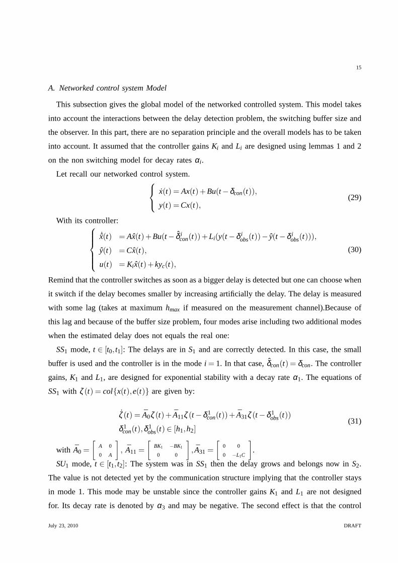
Fig. 2. Switch among four modes.

To summarize:

SS1 : t ∈ [t0, t1] i = 1, Bu f f er= h2−T δcon(t) = δcon(t) δcon(t) ∈ S1, δobs(t) ∈ S1

SU1 : t ∈ [t1, t2] i = 1, Bu f f er= h2−T δcon(t) 6= δcon(t) δcon(t) ∈ S2, δobs(t) ∈ S2

SS2 : t ∈ [t2, t3] i = 2, Bu f f er= h3−T δcon(t) = δcon(t) δcon(t) ∈ S2, δobs(t) ∈ S2

SU2 : t ∈ [t3, t4] i = 2, Bu f f er= h3−T δcon(t) = δcon(t) δcon(t) ∈ S2, δobs(t) ∈ S1

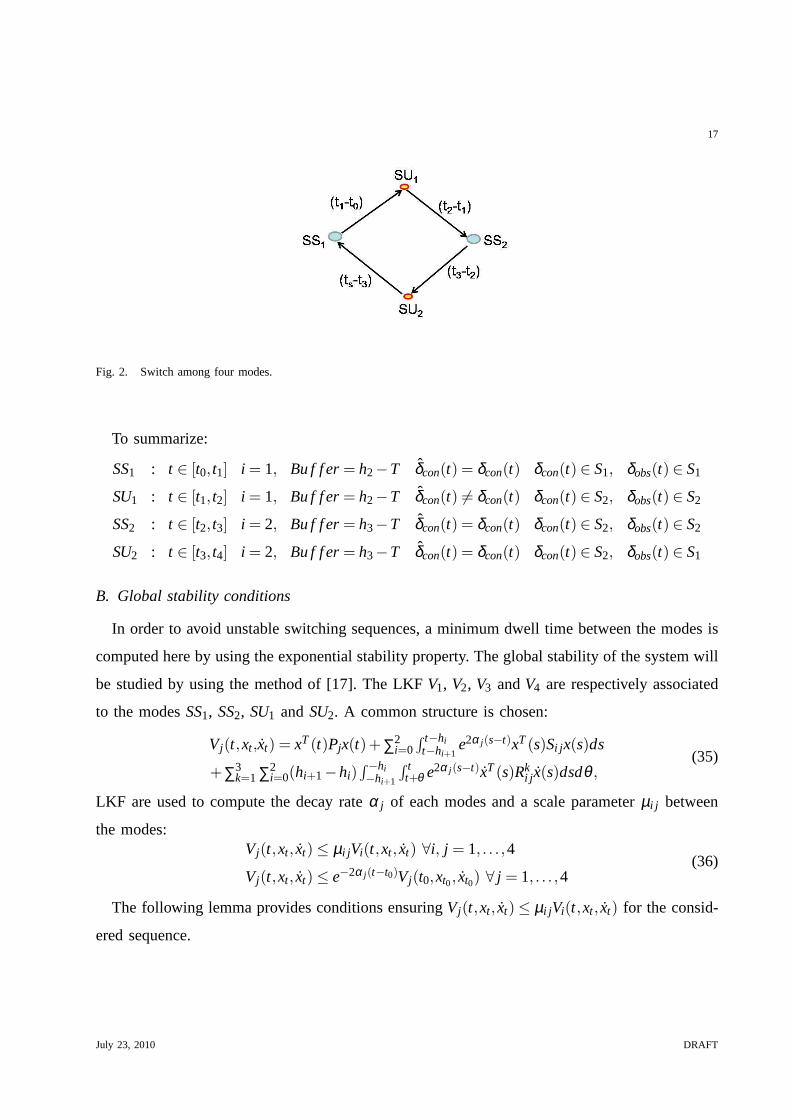
B. Global stability conditions

In order to avoid unstable switching sequences, a minimum dwell time between the modes is

computed here by using the exponential stability property.The global stability of the system will

be studied by using the method of [17]. The LKFV1, V2, V3 andV4 are respectively associated

to the modesSS1, SS2, SU1 andSU2. A common structure is chosen:

Vj(t,xt,xt) = xT(t)Pjx(t)+∑2i=0

∫ t−hit−hi+1

e2α j (s−t)xT(s)Si j x(s)ds

+∑3k=1 ∑2

i=0(hi+1−hi)∫−hi−hi+1

∫ tt+θ e2α j (s−t)xT(s)Rk

i j x(s)dsdθ ,(35)

LKF are used to compute the decay rateα j of each modes and a scale parameterµi j between

the modes:Vj(t,xt, xt) ≤ µi jVi(t,xt, xt) ∀i, j = 1, . . . ,4

Vj(t,xt, xt) ≤ e−2α j (t−t0)Vj(t0,xt0, xt0) ∀ j = 1, . . . ,4(36)

The following lemma provides conditions ensuringVj(t,xt, xt) ≤ µi jVi(t,xt, xt) for the consid-

ered sequence.

July 23, 2010 DRAFT

18

Fig. 3. Minimum dwell time: Small delay fromt0 to t1, then big delay fromt1 to t3, switches att2 and ts.

Lemma 3:The propertyVj(t,xt, xt) ≤ µi jVi(t,xt, xt), (i, j) ∈ {(1,4),(4,2),(2,3),(3,1)}} is

guaranteed if the following conditions are satisfied :

∀n∈ {0,1,2},∀h∈ {hn,hn+1},∀k∈ {1,2,3}

Pi ≤ µi j Pj

∀(i, j) ∈ {(1,4),(4,2),(2,3),(3,1)}, ,

e−2αihSni ≤ µi j e−2α jhSn j,

e−2αihRkni ≤ µi j e−2α jhRk

n j.

(37)

The computation of the parametersαi and µi j is done using the following lemma which is a

specific version of theorem 1.

Lemma 4:Given some scalarsα j and µi j , (i, j) ∈ {(1,4),(4,2),(2,3),(3,1)}, if there exist

scalarsµi j , i, j = 1, . . . ,4, matricesPj > 0, Rki j > 0 andSi j > 0(i = 0,1,2 andk = 1,2,3), P2 j , P3 j ,

Y1k j andY2k j ( j = 1,2,3,4 andk = 1,2,3) with proper dimensions, such that (38), (39) and (37)

conditions hold then the system (IV-A) has positive functionals (35) fulfilling 36.

Φ|SS1 =

[

Ψ11 Ψ21

∗ Ψ31

]

< 0, Φ|SS2 =

[

Ψ12 Ψ22

∗ Ψ32

]

< 0, (38)

Φ|SU1 =

[

Ψ13 Ψ23

∗ Ψ33

]

< 0, Φ|SU2 =

[

Ψ14 Ψ24

∗ Ψ34

]

< 0, (39)

July 23, 2010 DRAFT

19

where:

Ψ11 =

Φ111 Φ121 PT21A11+PT

21A31+∑3k=1(R

k01−YT

1k1) ∑3k=1YT

1k1 0

∗ Φ221 PT31A11+PT

31A31−∑3k=1YT

2k1 ∑3k=1YT

2k1 0

∗ ∗ S11− S01−∑3k=1 Rk

01 0 0

∗ ∗ ∗ S21− S11−∑3k=1 Rk

21 ∑3k=1 Rk

21

∗ ∗ ∗ ∗ −S21−∑3k=1 Rk

21

, (40)

Ψ21 =

YT111−PT

21A11 YT111 YT

121 YT121 YT

131−PT21A31 YT

131

YT211−PT

31A11 YT211 YT

221 YT221 YT

231−PT31A31 YT

231

0 0 0 0 0 0

0 0 0 0 0 0

0 0 0 0 0 0

, (41)

Ψ31 =

−R111 0 0 0 0 0

∗ −R111 0 0 0 0

∗ ∗ −R211 0 0 0

∗ ∗ ∗ −R211 0 0

∗ ∗ ∗ ∗ −R311 0

∗ ∗ ∗ ∗ ∗ −R311

, (42)

Ψ12 =

Φ112 Φ122 ∑3k=1 Rk

02 PT22A12+PT

21A31−∑3k=1YT

1k2 ∑3k=1YT

1k2

∗ Φ222 0 PT32A12+PT

32A32−∑3k=1(Y

T2k2) ∑3

k=1YT2k2

∗ ∗ S12− S02−∑3k=1(R

k02+ Rk

12) ∑3k=1 Rk

12 0

∗ ∗ ∗ S22− S12−∑3k=1 Rk

12 0

∗ ∗ ∗ ∗ −S22

, (43)

Ψ22 =

YT112−PT

22A12 YT112 YT

122 YT122 YT

132−PT22A32 YT

132

YT212−PT

32A12 YT212 YT

222 YT222 YT

232−PT32A32 YT

232

0 0 0 0 0 0

0 0 0 0 0 0

0 0 0 0 0 0

, (44)

Ψ32 =

−R122 0 0 0 0 0

∗ −R122 0 0 0 0

∗ ∗ −R222 0 0 0

∗ ∗ ∗ −R222 0 0

∗ ∗ ∗ ∗ −R322 0

∗ ∗ ∗ ∗ ∗ −R322

, (45)

Ψ13 =

Φ113 Φ123 ∑3k=1 Rk

03+PT23A13−YT

113 PT23(A23+ A33)+YT

113−YT123−YT

133 YT123+YT

133

∗ Φ223 PT33A13−YT

213 PT33A23+PT

33A33+YT213−YT

223−YT233 YT

223+YT233

∗ ∗ S13− S03−∑3k=1 Rk

03− R213− R3

13 R213+ R3

13 0

∗ ∗ ∗ S23− S13− R123− R2

13− R313 R1

23 0

∗ ∗ ∗ ∗ −S23− R123

, (46)

Ψ23 =

YT113−PT

23A13 YT113 YT

123−PT23A23 YT

123 YT133−PT

23A33 YT133

YT213−PT

33A13 YT213 YT

223−PT33A23 YT

223 YT233−PT

33A33 YT233

0 0 0 0 0 0

0 0 0 0 0 0

0 0 0 0 0 0

, (47)

July 23, 2010 DRAFT

20

Ψ33 =

−R113 0 0 0 0 0

∗ −R113 0 0 0 0

∗ ∗ −R223 0 0 0

∗ ∗ ∗ −R223 0 0

∗ ∗ ∗ ∗ −R323 0

∗ ∗ ∗ ∗ ∗ −R323

, (48)

Ψ14 =

Φ114 Φ124 ∑3k=1 Rk

04+PT24A34−YT

134 PT24A14+YT

134−YT114−YT

124 YT114+YT

124

∗ Φ224 PT34A34−YT

234 PT34A14+YT

234−YT214−YT

224 YT214+YT

224

∗ ∗ S14− S04−∑2k=1(R

k04+ Rk

14)− R304 ∑2

k=1 Rk14 0

∗ ∗ ∗ S24− S14−∑2k=1 Rk

14− R324 R3

24

∗ ∗ ∗ ∗ −S24− R324

, (49)

Ψ24 =

YT114−PT

24A14 YT114 YT

124 YT124 YT

134−PT24A34 YT

134

YT214−PT

34A14 YT214 YT

224 YT224 YT

234−PT34A34 YT

234

0 0 0 0 0 0

0 0 0 0 0 0

0 0 0 0 0 0

, (50)

Ψ34 =

−R124 0 0 0 0 0

∗ −R124 0 0 0 0

∗ ∗ −R224 0 0 0

∗ ∗ ∗ −R224 0 0

∗ ∗ ∗ ∗ −R314 0

∗ ∗ ∗ ∗ ∗ −R314

, (51)

and where

Ri j = e−2α j (hi+1)Ri j ,

Si j = e−2α jhi+1Si j ,

Si j = e−2α jhi Si j ,

Φ11j = ATP2 j +PT2 jA+S0 j −e−2α jh1R0 j +2α jPj ,

Φ12j = Pj −PT2 j +ATP3 j , Φ22j = −P3 j −PT

3 j +∑2i=0(hi+1−hi)

2Ri j .

(52)

�

Since the NCS global model switches are in a predetermined order, the global performance/stability

is achieved if a one of the functionalVj is decreasing each cycle. This gives the following

condition to ensure a decay rateαg over a complete cycle:V1(ts,xts, xts)≤e−2α j (ts−t0)V1(t0,xt0, xt0).

This condition is illustrated on figure 3. The following theorem gives the stability conditions for

a 4 sequenced mode switching system.

system (IV-A) has positive functionals (35) fulfilling 36.

July 23, 2010 DRAFT

21

Theorem 2:Consider a 4 sequenced mode switching model described in (IV-A). Given some

scalarsα j and µi j , (i, j) ∈ {(1,4),(4,2),(2,3),(3,1)}, if there exist scalarsµi j , i, j = 1, . . . ,4,

matricesPj > 0, Rki j > 0 andSi j > 0(i = 0,1,2 andk= 1,2,3), P2 j , P3 j , Y1k j andY2k j ( j = 1,2,3,4

and k = 1,2,3) with proper dimensions, such that (37), (38), (39) and condition (53) hold for

someαg > 0 then the model (IV-A) is exponentially stable with the decay rateαg :

µ14µ42µ23µ31e−2α4(ts−t3)−2α2(t3−t2)−2α3(t2−t1)−2α1(t1−t0) ≤ eαg(ts−t0) (53)

Proof: Using the properties (36), it comes:

V1(ts,xts,xts) ≤ µ14V4(ts,xts,xts)

≤ µ14e−2α4(ts−t3)V4(t3,xt3,xt3)

≤ µ14µ42e−2α4(ts−t3)V2(t3,xt3,xt3)

≤ µ14µ42e−2α2(ts−t2)−2α2(t3−t2)V2(t2,xt2,xt2)

...

≤ µ14µ42µ23µ31e−2α4(ts−t3)−2α2(t3−t2)−2α3(t2−t1)−2α1(t1−t0)V1(t0,xt0,xt0).

(54)

thenV1(ts,xts, xts) ≤ e−2α j (ts−t0)V1(t0,xt0, xt0) if

µ14µ42µ23µ31e−2α4(ts−t3)−2α2(t3−t2)−2α3(t2−t1)−2α1(t1−t0) ≤ eαg(ts−t0) (55)

Remark 5:There is always a solution to the problem of finding the switchtime ts in the two

following cases:

1) αg < α4 even in the case of fugitive modes,

2) αg < α1 if the dwell time in modeSS1 is sufficient.

This result could be used to provide recommendation, in the form of dwell time inSS1 mode

to choose the network type needed to achieved given performances.

Note that the conditions given in corollary 4 and in theorem 2are not strictly LMI since the

α j and theµi j must be fixed. A successive optimization of the parameters can be achieved to

get a compromise between a high values ofα j and low valuesµi j . This optimization is possible

since the conditions are harder to satisfy whenα j grows / µi j decreases.

The global approach for the switching controller design is summarized in the following

algorithm:

July 23, 2010 DRAFT

22

Algorithm 1: Controller design steps:

1) use lemmas 1 and 2 to compute the gains with givenα performances for modes 1 and 2.

2) use corollary 4 to compute a compromise between the minimum µi j and the maximumαi .

3) implement the controller (7) that uses the following switching law:

i ={ 1, if δobs(t)) ∈ S1 and t > ts

2, otherwise.(56)

ts is extracted by applying the logarithm function on the condition of theorem 2.

Remark 6:These result does not take into account the packet dropout case for sake of clarity.

Since the presented controller does not detect packet dropouts, it is treated using [30] to compute

de worst case exponential decay rate for all modes. Remark also that these results can be extended

to more zones and to the case where the control delay range is different from the observer delay

range.

V. EXPERIMENTAL RESULTS

The experiments are done on two computers separated from about 40 kilometers away (Fig.

4). The Master program runs on the remote computer with an advanced computing capability,

the Slave one on the local one which also communicates with a light-inertia robot Miabot of

the company Merlin by Bluetooth.

Fig. 4. Structure of the global system

A. The structure of the Master

In order to implement the model for the remote control system, a four-threads program is

designed to fulfill the functions of Controller and Observerin Fig.4, while the explication of all

the parameters refers to [15].

July 23, 2010 DRAFT

23

ConsThread

SenderThread

ReceiverThread

ObserverThread

File consign Slave

Slave

consTab

c(t3,p)

u(tm,k), tm,k

y(ts,k′), ts,k′ −d1

y(ts,k′), ts,k′ −d1x(t0,q)

x(t0,q)

u(tm,k), tm,k

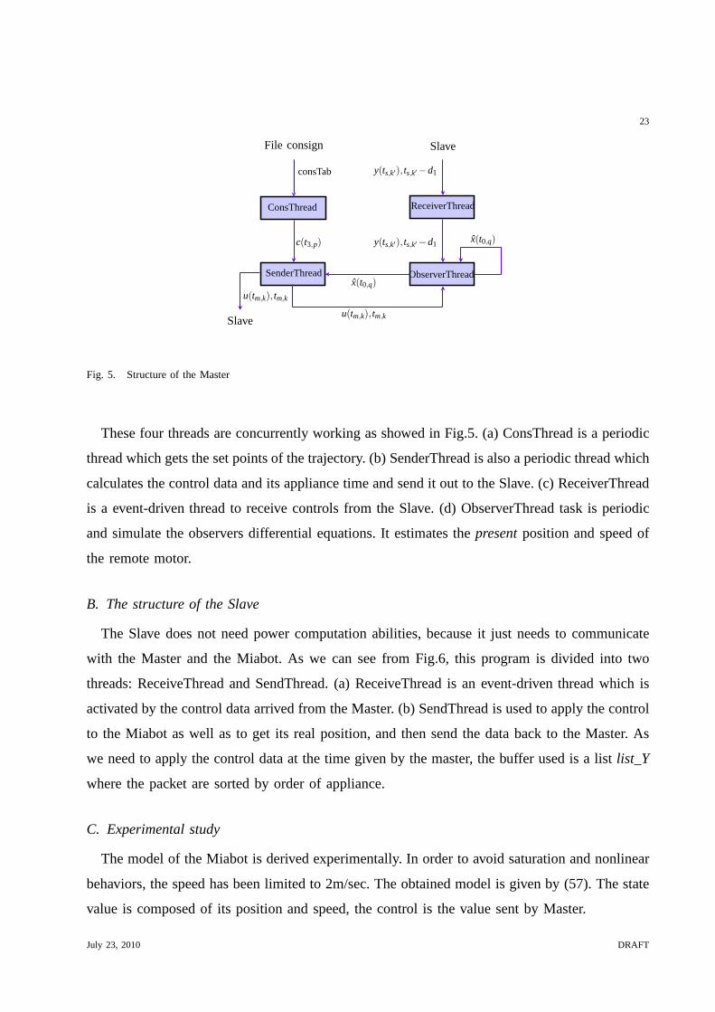
Fig. 5. Structure of the Master

These four threads are concurrently working as showed in Fig.5. (a) ConsThread is a periodic

thread which gets the set points of the trajectory. (b) SenderThread is also a periodic thread which

calculates the control data and its appliance time and send it out to the Slave. (c) ReceiverThread

is a event-driven thread to receive controls from the Slave.(d) ObserverThread task is periodic

and simulate the observers differential equations. It estimates thepresentposition and speed of

the remote motor.

B. The structure of the Slave

The Slave does not need power computation abilities, because it just needs to communicate

with the Master and the Miabot. As we can see from Fig.6, this program is divided into two

threads: ReceiveThread and SendThread. (a) ReceiveThreadis an event-driven thread which is

activated by the control data arrived from the Master. (b) SendThread is used to apply the control

to the Miabot as well as to get its real position, and then sendthe data back to the Master. As

we need to apply the control data at the time given by the master, the buffer used is a listlist_Y

where the packet are sorted by order of appliance.

C. Experimental study

The model of the Miabot is derived experimentally. In order to avoid saturation and nonlinear

behaviors, the speed has been limited to 2m/sec. The obtained model is given by (57). The state

value is composed of its position and speed, the control is the value sent by Master.

July 23, 2010 DRAFT

24

ReceiveThread

SendThread Miabot

Master

Master

u(tm,k), tm,k

y(ts,k′), ts,k′ −d1

y(ts,k′), ts,k′ −d1

u(tm,k), tm,k+h1m

Fig. 6. Structure of the Slave

x(t) =

[

0 1

0 −10

]

x(t)+

[

0

0.024

]

u(t −δcon(t))

y(t) =[

1 0]

x(t).(57)

Some delay measurement has been done between the master and the slave. During a day,

the RTT (Round-trip-time=twice the communication delay) measured using the ICMP (Internet

Control Message [25]) belonged to[4.1ms577ms] with an average value of 52.37ms. During the

experimental time, the delay was oscillating between an average value of 40msand 100ms. Taking

into account these information, considering also the Bluetooth transmission delays (considered

constant) and the sampling delays, we takeS1 = [0.01,0.08[ and S2 = [0.08,0.5] for the delay

subset. Any packet data delayed by more than 0.5secis considered lost.

According to Lemma (1) and (2), the maximum exponential convergence ensuring the modes

stability are:αc1 = 3.8, αo

1 = 4.49, αc2 = αo

2 = 0.72. The corresponding control gains are too

high to keep the speed lower than 2m/sec. To avoid actuator saturation and nonlinear behavior

when the robot speed is too high, smaller gains are computed considering the following values

: αc1 = 2, αo

1 = 2.5, αc2 = 0.6 andαo

2 = 0.72.

The resulting gainsKi andLi (i = 1,2) are given by:[

L1 L2

]

=

−7.06 −1.44

0.04 −0.01

,

K1

K2

=

−1485 −461

−99 1

. (58)

Remark 7:Note that speed related component of the control gainK2 has a positive value.

This just mean that to keep the system stability when the delay is high, it is needed slightly

degrade the performances of the system stable open-loop pole.

July 23, 2010 DRAFT

25

Once the gain are computed, the dwell time parametersαi and µi j are computed following

theses steps:

1) The values ofα3 andα4 are maximized for fixedµi j = 100,α1 andα2, satisfying corollary

4 conditions.

2) µi j are minimized using the criterionµ14+ µ42+ µ23+ µ31 for the obtainedαi and LKF

matrices, satisfying corollary 4 conditions.

These steps lead to the following solutions:α1 = 2,α2 = 0.6,α3 = −4,α4 = 0.6. The global

performanceαg chosen is chosen to only keep stability:αg = 0.

D. Results of remote experiment

The result is shown in Fig.7, in which the blue curve represents the set values; the green

and red represent respectively the robot’s estimated position and speed; the black corresponds

to the real position of the Miabot. Fig.8 illustrate the corresponding switched control signals

from Master to Slave. The red curve is the real control while the green and the black ones

are the controls calculated respectively for the two subsystems. We can see the switch points

according to the values of time-delay. Fig.9 depicts the variable global time-delays on the control

communication channel and the corresponding switching signal.

On Fig.7, one can notice three kinds of step responses. The first one corresponds to the case

when the time-delay is greater than 80ms, only the second subsystem is active. In this case,

a decay rateα2 is guaranteed. During the second step, only the first mode is active because

delays are small. The performances are better: the responsetime is smaller since a decay rate of

α1 is achieved. In the last kind of response, where a some switches occur during the transient

response. In that case, only the global stability is guaranteed. At the momentt ∈ [42ms45ms],

the time-delay becomes small, but the switching strategy ()do not permit to switch back to

mode 1 in order to guarantee the global stability.

Remark 8:Notice that despite the fact that the observer is based on delays measurements, it

this keep a good estimation on the present state of the slave.

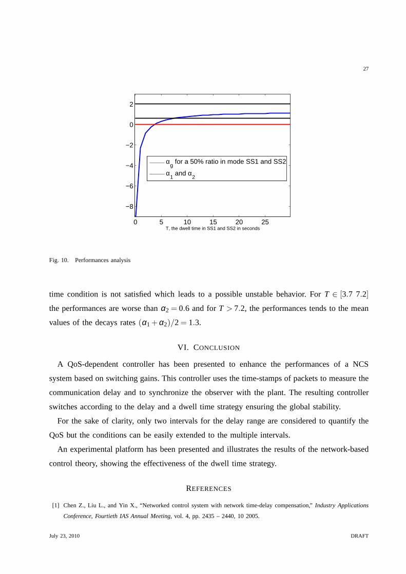
The last figure (Fig.10) provides a performance analysis in term of global decay rateαg over

one cycle (SS1 → SU1 → SS2 → SU2 → SS1). It is assumed that the dwell time in the modes

SU1 andSU2 are fixed to the maximum delay, i.e. 0.5s. The figure gives the lower boundαg

according the the dwell timeT in the modesSS1 and SS2. For T ≤ 3.7 the controller dwell

July 23, 2010 DRAFT

26

0 5 10 15 20 25 30 35 40 45 50 55−1

−0.8

−0.6

−0.4

−0.2

0

0.2

0.4

0.6

0.8

1

time(s)

Posi

tion(

m)

Tasks^x

1(t

k)

^x2(t

k)

y.dis

Fig. 7. Results of remote experiment

0 5 10 15 20 25 30 35 40 45 50 55−800

−600

−400

−200

0

200

400

600

800

time(s)

Con

trol(u

)

u1(K

1,L

1)

u2(K

2,L

2)

Control(u)

Fig. 8. The corresponding switched control

0 5 10 15 20 25 30 35 40 45 50 550

20

40

60

80

100

120

140

time (s)

Time−

delay

(ms)

Fig. 9. The corresponding variable time-delays and signalsof switching

July 23, 2010 DRAFT

27

0 5 10 15 20 25

−8

−6

−4

−2

0

2

T, the dwell time in SS1 and SS2 in seconds

αg for a 50% ratio in mode SS1 and SS2

α1 and α

2

Fig. 10. Performances analysis

time condition is not satisfied which leads to a possible unstable behavior. ForT ∈ [3.7 7.2]

the performances are worse thanα2 = 0.6 and forT > 7.2, the performances tends to the mean

values of the decays rates(α1+α2)/2 = 1.3.

VI. CONCLUSION

A QoS-dependent controller has been presented to enhance the performances of a NCS

system based on switching gains. This controller uses the time-stamps of packets to measure the

communication delay and to synchronize the observer with the plant. The resulting controller

switches according to the delay and a dwell time strategy ensuring the global stability.

For the sake of clarity, only two intervals for the delay range are considered to quantify the

QoS but the conditions can be easily extended to the multipleintervals.

An experimental platform has been presented and illustrates the results of the network-based

control theory, showing the effectiveness of the dwell timestrategy.

REFERENCES

[1] Chen Z., Liu L., and Yin X., “Networked control system with network time-delay compensation,”Industry Applications

Conference, Fourtieth IAS Annual Meeting, vol. 4, pp. 2435 – 2440, 10 2005.

July 23, 2010 DRAFT

28

[2] Chiasson J. and Loiseau J.J.,Applications of time delay systems. Springer, 2007, vol. 352.

[3] Estrada-Garcia H.J., Marquez-Martinez L.A., and Moog C.H., “Master-slave synchronization for two inverted pendulums

with communication time-delay,”7th IFAC workshop on time delay systems, Nantes, France, 2007.

[4] Fattouh A. and Sename O., “H∞-based impedance control of teleoperation systems with time delay,” 4th Workshop on

Time Delay Systems, 9 2003.

[5] Fridman E., “New Lyapunov-Krasovskii functionals for stability of linear retarded and neutral type systems,”Systems&

Control Letters, vol. 43, pp. 309–319, 2001.

[6] Fridman E., Seuret A., and Richard J.-P., “Robust sampled-data stabilization of linear systems: an input delay approach,”

Automatica, vol. 40, pp. 1441–1446, 2004.

[7] Gao H., Chen T., and Lam J., “A new delay system approach tonetwork-based control,”Automatica, vol. 44, no. 1, pp.

39–52, 2008.

[8] Georges J.-P., Divoux T., and Rondeau E., “Confronting the performances of a switched ethernet network with industrial

constraints by using the network calculus,”International Journal of Communication Systems(IJCS), vol. 18, no. 9, pp.

877–903, 2005.

[9] Gu K., Kharitonov V., and Chen J., “Stability of time-delay systems,”Birkhauser: Boston, 2003.

[10] He Y., Wu M., She J.H., and Liu G.P., “Parameter-dependent lyapunov functional for stability of time-delay systemswith

polytopic-type uncertainties,”IEEE Transactions on Automatic Control, vol. 49, pp. 828–832, 2004.

[11] Hespanha J.P. and Morse A.S., “stability of switched systems with average dwell-time,”Proceedings of the38th Conference

on Decision& Control, pp. 2655–2660, December 1999.

[12] Hespanha J.P., Naghshtabrizi P., and Xu Y., “A survey ofrecent results in networked control systems,”Proceedings of the

IEEE, vol. 95, pp. 138–162, January 2007.

[13] Hirche S., Chen C.-C, and Buss M, “Performance orientedcontrol over networks -switching controllers and switchedtime

delay-,” Proceedings of the 45th IEEE Conference on Decision& Control, December 2006.

[14] Huang J.Q. and Lewis F.L., “Neural-network predictivecontrol for nonlinear dynamic systems with time delays,”IEEE

Transactions on Neural Networks, vol. 14, no. 2, pp. 377–389, 2003.

[15] Jiang W.-J., Kruszewski A., Richard J.-P., and Toguyeni A., “A gain scheduling strategy for the control and estimation of

a remote robot via internet,”The 27th Chinese Control Conference, July 2008.

[16] Lelevé A., Fraisse P., and Dauchez P., “Telerobotics over IP networks: Towards a low-level real-time architecture,” IROS’01

International conference on intelligent robots and systems,Maui,Hawaii, October 2001.

[17] Liberzon D.,Switching in Systems and Control, T. Basar, Ed. Birkhäuser, 2003.

[18] Mills D.L., “Improved algorithms for synchronizing computer network clocks,”IEEE/ACM Transactions On Networking,

vol. 3, no. 3, pp. 245–254, June 1995.

[19] Niculescu S.-I.,Delay effects on stability: a robust control approach. Springer, 2001, vol. 269.

[20] Niemeyer G. and Slotine J.-J., “Towards force-reflecting teleoperation over the internet,”IEEE Int. Con. on Robotics&

Automation, 1998.

[21] Nilsson J., “Real-time control systems with delays,”Ph.d. thesis at the department of automatic control. Lund Institute of

Technology. Sweden, 1998.

[22] Nilsson J., Bernhardsson B., and Wittenmark B., “Stochastic analysis and control of real-time control systems with random

time delay.”Automatica, vol. 34, no. 1, pp. 57–64, 1998.

July 23, 2010 DRAFT

29

[23] Ploplys N.J., Kawka P.A., and Alleyne A.G., “Closed-loop control over wireless networks,”IEEE Control Systems

Magazine, June 2004.

[24] J. Postel, “User datagram protocol,”USC/Information Sciences Institute, RFC 768, 1980.

[25] ——, “Internet control message protocol,”USC/Information Sciences Institute, RFC 792, 1981.

[26] Richard J.-P., “Time delay systems: an overview of somerecent advances and open problems,”Automatica, vol. 39, pp.

1667–1694, 2003.

[27] Richard J.-P. and Divoux T.,Systèmes commandés en réseau. Hermes-Lavoisier, IC2, Systèmes Automatisés, 2007.

[28] Seuret A., Fridman E., and Richard J.-P., “Sampled-data exponential stabilization of neutral systems with input and state

delays,”Proc. of IEEE MED 2005, 13th Mediterranean Conference on Control and Automation, Cyprus, 2005.

[29] Seuret A., Michaut F., Richard J.-P., and Divoux T., “Networked control using gps synchronization,”Proc. of ACC06,

American Control Conf., Mineapolis, USA, June 2006.

[30] Seuret A. and Richard J.-P., “Control of a remote systemover network including delays and packet dropout,”IFAC World

Congress, Seoul, Korea, July 2008.

[31] Sun X.-M., Zhao J., and Hill D., “Stability andl2-gain analysis for switched delay systems,”Automatica, vol. 42, pp.

1769–1774, 2006.

[32] Sun Y.G. and Wang L., “Stability of switched systems with time-varying delays: delay-dependent common lyapunov

functional approach,”Proceedings of the 2006 American Control Conference, June 2006.

[33] Tipsuwan Y. and Chow M.-Y., “Control methodologies in network control systems,”Control Engineering Practice, vol. 11,

pp. 1099–1011, 2003.

[34] Witrant E., Canudas-De-Wit C., and Georges D., “Remotestabilization via communication networks with a distributed

control law,” IEEE Transactions on Automatic control, 2007.

[35] Yan P. and Özbay H., “Stability analysis of switched time delay systems,”SIAM Journal on Control and Optimization,

vol. 47, no. 2, pp. 936–949, 2008.

[36] Yu M., Wang L., and Chu T., “An LMI approach to network control systems with data packet dropout and transmission

delays,”MTNS ’04 Proc. of Mathematical Theory Networks and Systems,Leuven, Belgium, 2004.

[37] Zampieri S., “Trends in networked control systems,”Proceedings of the 17th World Congress, The International federation

of Automatic Control, July 2008.

[38] Zhang W.A. and Yu L., “Modelling and control of networked control systems with both network-induced delay and

packet-dropout,”Automatica, vol. 44, pp. 3206–3210, 2008.

July 23, 2010 DRAFT