a survey of outlier detection methodologies

A Survey of Outlier Detection Methodologies

VICTORIA J. HODGE & JIM AUSTINDepartment of Computer Science, University of York, York, YO10 5DD UK(E-mail: fvicky, [email protected])

Abstract. Outlier detection has been used for centuries to detect and, where appropri-ate, remove anomalous observations from data. Outliers arise due to mechanical faults,

changes in system behaviour, fraudulent behaviour, human error, instrument error orsimply through natural deviations in populations. Their detection can identify systemfaults and fraud before they escalate with potentially catastrophic consequences. It can

identify errors and remove their contaminating effect on the data set and as such topurify the data for processing. The original outlier detection methods were arbitrary butnow, principled and systematic techniques are used, drawn from the full gamut of

Computer Science and Statistics. In this paper, we introduce a survey of contemporarytechniques for outlier detection. We identify their respective motivations and distinguishtheir advantages and disadvantages in a comparative review.

Keywords: anomaly, detection, deviation, noise, novelty, outlier, recognition

1. Introduction

Outlier detection encompasses aspects of a broad spectrum of tech-niques. Many techniques employed for detecting outliers are funda-mentally identical but with different names chosen by the authors. Forexample, authors describe their various approaches as outlier detection,novelty detection, anomaly detection, noise detection, deviation detec-tion or exception mining. In this paper, we have chosen to call thetechnique outlier detection although we also use novelty detection wherewe feel appropriate but we incorporate approaches from all five cate-gories named above. Additionally, authors have proposed many defi-nitions for an outlier with seemingly no universally accepted definition.We will take the definition of Grubbs (1969) and quoted in Barnett andLewis (1994).

An outlying observation, or outlier, is one that appears to deviatemarkedly from other members of the sample in which it occurs.

Artificial Intelligence Review 22: 85–126, 2004.� 2004 Kluwer Academic Publishers. Printed in the Netherlands.

85

A further outlier definition from Barnett and Lewis (1994) is:

An observation (or subset of observations) which appears to beinconsistent with the remainder of that set of data.

In Figure 2, there are five outlier points labelled V, W, X, Y and Zwhich are clearly isolated and inconsistent with the main cluster ofpoints. The data in the figures in this survey paper is adapted from theWine data set (Blake and Merz, 1998).

John (1995) states that an outlier may also be ‘surprising veridicaldata’, a point belonging to class A but actually situated inside class Bso the true (veridical) classification of the point is surprising to theobserver. Aggarwal and Yu (2001) note that outliers may be con-sidered as noise points lying outside a set of defined clusters oralternatively outliers may be defined as the points that lie outside ofthe set of clusters but are also separated from the noise. These outliersbehave differently from the norm. In this paper, we focus on the twodefinitions quoted from Barnett and Lewis (1994) above and do notconsider the dual class-membership problem or separating noise andoutliers.

Outlier detection is a critical task in many safety critical environ-ments as the outlier indicates abnormal running conditions from whichsignificant performance degradation may well result, such as an aircraftengine rotation defect or a flow problem in a pipeline. An outlier candenote an anomalous object in an image such as a land mine. An outliermay pinpoint an intruder inside a system with malicious intentions sorapid detection is essential. Outlier detection can detect a fault on afactory production line by constantly monitoring specific features of theproducts and comparing the real-time data with either the features ofnormal products or those for faults. It is imperative in tasks such ascredit card usage monitoring or mobile phone monitoring to detect asudden change in the usage pattern which may indicate fraudulent usagesuch as stolen card or stolen phone airtime. Outlier detection accom-plishes this by analysing and comparing the time series of usage sta-tistics. For application processing, such as loan application processingor social security benefit payments, an outlier detection system candetect any anomalies in the application before approval or payment.Outlier detection can additionally monitor the circumstances of a ben-efit claimant over time to ensure the payment has not slipped into fraud.Equity or commodity traders can use outlier detection methods tomonitor individual shares or markets and detect novel trends which mayindicate buying or selling opportunities. A news delivery system can

VICTORIA J. HODGE AND JIM AUSTIN86

detect changing news stories and ensure the supplier is first with thebreaking news. In a database, outliers may indicate fraudulent cases orthey may just denote an error by the entry clerk or a misinterpretationof a missing value code, either way detection of the anomaly is vital fordata base consistency and integrity.

A more exhaustive list of applications that utilise outlier detection is:– Fraud detection – detecting fraudulent applications for credit cards,state benefits or detecting fraudulent usage of credit cards or mobilephones.

– Loan application processing – to detect fraudulent applications orpotentially problematical customers.

– Intrusion detection – detecting unauthorised access in computernetworks.

– Activity monitoring – detecting mobile phone fraud by monitoringphone activity or suspicious trades in the equity markets.

– Network performance – monitoring the performance of computernetworks, for example to detect network bottlenecks.

– Fault diagnosis – monitoring processes to detect faults in motors,generators, pipelines or space instruments on space shuttles forexample.

– Structural defect detection – monitoring manufacturing lines to detectfaulty production runs for example cracked beams.

– Satellite image analysis – identifying novel features or misclassifiedfeatures.

– Detecting novelties in images – for robot neotaxis or surveillancesystems.

– Motion segmentation – detecting image features moving indepen-dently of the background.

– Time-series monitoring – monitoring safety critical applications suchas drilling or high-speed milling.

– Medical condition monitoring – such as heart-rate monitors.– Pharmaceutical research – identifying novel molecular structures.– Detecting novelty in text – to detect the onset of news stories, fortopic detection and tracking or for traders to pinpoint equity, com-modities, FX trading stories, outperforming or under performingcommodities.

– Detecting unexpected entries in databases – for data mining to detecterrors, frauds or valid but unexpected entries.

– Detecting mislabelled data in a training data set.Outliers arise because of human error, instrument error, natural

deviations in populations, fraudulent behaviour, changes in behaviour

OUTLIER DETECTION METHODOLOGIES 87

of systems or faults in systems. How the outlier detection systemdeals with the outlier depends on the application area. If the outlierindicates a typographical error by an entry clerk then the entry clerkcan be notified and simply correct the error so the outlier will berestored to a normal record. An outlier resulting from an instrumentreading error can simply be expunged. A survey of human populationfeatures may include anomalies such as a handful of very tall people.Here the anomaly is purely natural, although the reading may beworth flagging for verification to ensure no errors, it should be in-cluded in the classification once it is verified. A system should use aclassification algorithm that is robust to outliers to model data withnaturally occurring outlier points. An outlier in a safety criticalenvironment, a fraud detection system, an image analysis system oran intrusion monitoring system must be detected immediately (inreal-time) and a suitable alarm sounded to alert the system admin-istrator to the problem. Once the situation has been handled, thisanomalous reading may be stored separately for comparison with anynew fraud cases but would probably not be stored with the mainsystem data as these techniques tend to model normality and use thisto detect anomalies.

There are three fundamental approaches to the problem of outlierdetection:1. Type 1 – Determine the outliers with no prior knowledge of the data.

This is essentially a learning approach analogous to unsupervisedclustering. The approach processes the data as a static distribution,pinpoints the most remote points, and flags them as potential outliers.Type 1 assumes that errors or faults are separated from the ‘normal’data and will thus appear as outliers. In Figure 3, points V, W, X, Yand Z are the remote points separated from the main cluster andwould be flagged as possible outliers. We note that the main clustermay be subdivided if necessary into more than one cluster to allowboth classification and outlier detection as with Figure 4. The ap-proach is predominantly retrospective and is analogous to a batch-processing system. It requires that all data be available beforeprocessing and that the data is static. However, once the systempossesses a sufficiently large database with good coverage, then it cancompare new items with the existing data. There are two sub-tech-niques commonly employed, diagnosis and accommodation (Rous-seeuw and Leroy, 1996). An outlier diagnostic approach highlights thepotential outlying points. Once detected, the systemmay remove theseoutlier points from future processing of the data distribution. Many


diagnostic approaches iteratively prune the outliers and fit their sys-tem model to the remaining data until no more outliers are detected.An alternative methodology is accommodation that incorporates theoutliers into the distribution model generated and employs a robustclassification method. These robust approaches can withstand out-liers in the data and generally induce a boundary of normalityaround the majority of the data which thus represents normalbehaviour. In contrast, non-robust classifier methods produce rep-resentations which are skewed when outliers are left in. Non-robustmethods are best suited when there are only a few outliers in the dataset (as in Figure 3) as they are computationally cheaper than therobust methods but a robust method must be used if there are a largenumber of outliers to prevent this distortion. Torr and Murray(1993) use a cheap Least Squares algorithm if there are only a fewoutliers but switch to a more expensive but robust algorithm forhigher frequencies of outliers.

2. Type 2 – Model both normality and abnormality. This approach isanalogous to supervised classification and requires pre-labelled data,tagged as normal or abnormal. In Figure 4, there are three classes ofnormal data with pre-labelled outliers in isolated areas. The entirearea outside the normal class represents the outlier class. The normalpoints could be classified as a single class or subdivided into the threedistinct classes according to the requirements of the system to pro-vide a simple normal/abnormal classification or to provide anabnormal and 3-classes of normally classifier.Classifiers are best suited to static data as the classification needs tobe rebuilt from first principles if the data distribution shifts unless thesystem uses an incremental classifier such as an evolutionary neuralnetwork. We describe one such approach later which uses a growwhen required (Marsland, 2001) network. A type 2 approach can beused for on-line classification, where the classifier learns the classi-fication model and then classifies new exemplars as and when re-quired against the learned model. If the new exemplar lies in a regionof normality it is classified as normal, otherwise it is flagged as anoutlier. Classification algorithms require a good spread of bothnormal and abnormal data, i.e., the data should cover the entiredistribution to allow generalisation by the classifier. New exemplarsmay then be classified correctly as classification is limited to a‘known’ distribution and a new exemplar derived from a previouslyunseen region of the distribution may not be classified correctly


unless the generalisation capabilities of the underlying classificationalgorithm are good.

3. Type 3 - Model only normality or in a very few cases modelabnormality (Japkowicz et al., 1995; Fawcett and Provost 1999).Authors generally name this technique novelty detection or noveltyrecognition. It is analogous to a semi-supervised recognition ordetection task and can be considered semi-supervised as the normalclass is taught but the algorithm learns to recognise abnormality. Theapproach needs pre-classified data but only learns data markednormal. It is suitable for static or dynamic data as it only learns oneclass which provides the model of normality. It can learn the modelincrementally as new data arrives, tuning the model to improve the fitas each new exemplar becomes available. It aims to define aboundary of normality.A type 3 system recognises a new exemplar as normal if it lies withinthe boundary and recognises the new exemplar as novel otherwise. InFigure 5, the novelty recogniser has learned the same data as shownin Figure 2 but only the normal class is learned and a boundary ofnormality induced. If points V, W, X, Y and Z from Figure 2 arecompared to the novelty recogniser they will be labelled as abnormalas they lie outside the induced boundary. This boundary may be hardwhere a point lies wholly within or wholly outside the boundary orsoft where the boundary is graduated depending on the underlyingdetection algorithm. A soft bounded algorithm can estimate the de-gree of ‘outlierness’.It requires the full gamut of normality to be available for training topermit generalisation. However, it requires no abnormal data fortraining unlike type 2. Abnormal data is often difficult to obtain orexpensive in many fault detection domains such as aircraft enginemonitoring. It would be extremely costly to sabotage an aircraftengine just to obtain some abnormal running data. Another problemwith type 2 is it cannot always handle outliers from unexpected re-gions, for example, in fraud detection a new method of fraud neverpreviously encountered or previously unseen fault in a machine maynot be handled correctly by the classifier unless generalisation is verygood. In this method, as long as the new fraud lies outside theboundary of normality then the system will be correctly detectthe fraud. If normality shifts then the normal class modelled by thesystem may be shifted by re-learning the data model or shifting themodel if the underlying modelling technique permits such as evolu-tionary neural networks.


The outlier approaches described in this survey paper generally mapdata onto vectors. The vectors comprise numeric and symbolic attri-butes to represent continuous-valued, discrete (ordinal), categorical(unordered numeric), ordered symbolic or unordered symbolic data.The vectors may be monotype or multi-type. The statistical and neuralnetwork approaches typically require numeric monotype attributes andneed to map symbolic data onto suitable numeric values1 but the ma-chine learning techniques described are able to accommodate multi-typevectors and symbolic attributes. The outliers are determined from the‘closeness’ of vectors using some suitable distance metric. Differentapproaches work better for different types of data, for different numbersof vectors, for different numbers of attributes, according to the speedrequired and according to the accuracy required. The two fundamentalconsiderations when selecting an appropriate methodology for an out-lier detection system are:– Selecting an algorithm which can accurately model the data distri-bution and accurately highlight outlying points for a clustering,classification or recognition type technique. The algorithm shouldalso be scalable to the data sets to be processed.

– Selecting a suitable neighbourhood of interest for an outlier. Theselection of the neighbourhood of interest is non-trivial. Manyalgorithms define boundaries around normality during processingand autonomously induce a threshold. However, these approachesare often parametric enforcing a specific distribution model or requireuser-specified parameters such as the number of clusters. Othertechniques discussed below require user-defined parameters to definethe size or density of neighbourhoods for outlier thresholding. Thechoice of neighbourhood whether user-defined or autonomously in-duced needs to be applicable for all density distributions likely to beencountered and can potentially include those with sharp densityvariations.In the remainder of this paper, we categorise and analyse broad

range of outlier detection methodologies. We pinpoint how each han-dles outliers and make recommendations for when each methodology isappropriate for clustering, classification and/or recognition. Barnett andLewis (1994) and Rousseeuw and Leroy (1996) describe and analyse abroad range of statistical outlier techniques and Marsland (2001)analyses a wide range of neural methods. We have observed that outlierdetection methods are derived from three fields of computing: statistics(proximity-based, parametric, non-parametric and semi-parametric),neural networks (supervised and unsupervised) and machine learning.


In the next four sections, we describe and analyse techniques from allthree fields and a collection of hybrid techniques that utilise algorithmsfrom multiple fields. The approaches described here encompass dis-tance-based, set-based, density-based, depth-based, model-based andgraph-based algorithms.

2. Statistical Models

Statistical approaches were the earliest algorithms used for outlierdetection. Some of the earliest are applicable only for single dimensionaldata sets. In fact, many of the techniques described in both Barnett andLewis (1994) and Rousseeuw and Leroy (1996) are single dimensional orat best univariate. One such single dimensional method is Grubbs’method (extreme studentized deviate) (Grubbs, 1969) which calculates aZ value as the difference between the mean value for the attribute andthe query value divided by the standard deviation for the attributewhere the mean and standard deviation are calculated from all attributevalues including the query value. The Z value for the query is comparedwith a 1% or 5% significance level. The technique requires no userparameters as all parameters are derived directly from data. However,the technique is susceptible to the number of exemplars in the data set.The higher the number of records the more statistically representativethe sample is likely to be.

Statistical models are generally suited to quantitative real-valueddata sets or at the very least quantitative ordinal data distributionswhere the ordinal data can be transformed to suitable numerical valuesfor statistical (numerical) processing. This limits their applicability andincreases the processing time if complex data transformations are nec-essary before processing.

Probably one of the simplest statistical outlier detection techniquesdescribed here, Laurikkala et al. (2000) use informal box plots topinpoint outliers in both univariate and multivariate data sets. Thisproduces a graphical representation (see Figure 1 for an example boxplot) and allows a human auditor to visually pinpoint the outlyingpoints. It is analogous to a visual inspection of Figure 2. Their ap-proach can handle real-valued, ordinal and categorical (no order)attributes. Box plots plot the lower extreme, lower quartile, median,upper quartile and upper extreme points. For univariate data, this is asimple 5-point plot, as in Figure 1. The outliers are the points beyondthe lower and upper extreme values of the box plot, such as V, Y and Z


in Figure 1. Laurikkala et al. suggest a heuristic of 1.5� inter-quartilerange beyond the upper and lower extremes for outliers but this wouldneed to vary across different data sets. For multivariate data sets

Figure 1. Shows a box plot of the y-axis values for the data in Figure 2 with the lowerextreme, the lower quartile, median, upper quartile and upper extreme from the normaldata and the three outliers V, Y and Z plotted. The points X and W from Figure 2 are

not outliers with respect to the y-axis values.

Figure 2. Shows a data distribution with 5 outliers (V, W, X, Y and Z). The data isadapted from the Wine data set (Blake and Merz, 1998).


the authors note that there are no unambiguous total orderings butrecommend using the reduced sub-ordering based on the generaliseddistance metric using the Mahalanobis distance measure (see equation(2)). The Mahalanobis distance measure includes the inter-attributedependencies so the system can compare attribute combinations. Theauthors found the approach most accurate for multivariate data wherea panel of experts agreed with the outliers detected by the system. Forunivariate data, outliers are more subjective and may be naturallyoccurring, for example the heights of adult humans, so there wasgenerally more disagreement. Box plots make no assumptions aboutthe data distribution model but are reliant on a human to note theextreme points plotted on the box plot.

Statistical models use different approaches to overcome the problemof increasing dimensionality which both increases the processing timeand distorts the data distribution by spreading the convex hull. Somemethods preselect key exemplars to reduce the processing time (Skalak,1994; Datta and Kibler, 1995). As the dimensionality increases, the datapoints are spread through a larger volume and become less dense. Thismakes the convex hull harder to discern and is known as the ‘Curse ofDimensionality’. The most efficient statistical techniques automaticallyfocus on the salient attributes and are able to process the higher numberof dimensions in tractable time. However, many techniques such ask-NN, neural networks, minimum volume ellipsoid or convex peelingdescribed in this survey are susceptible to the Curse of Dimensionality.These approaches may utilise a preprocessing algorithm to preselect thesalient attributes (Skalak and Rissland, 1990; Aha and Bankert, 1994;Skalak, 1994). These feature selection techniques essentially removenoise from the data distribution and focus the main cluster of normaldata points while isolating the outliers as with Figure 2. Only a fewattributes usually contribute to the deviation of an outlier case from anormal case. An alternative technique is to use an algorithm to projectthe data onto a lower dimensional subspace to compact the convex hull(Aggarwal and Yu, 2001) or use principal component analysis (Parraet al., 1996; Faloutsos et al., 1997).

2.1. Proximity-based techniques

Proximity-based techniques are simple to implement and make no priorassumptions about the data distribution model. They are suitable forboth type 1 and type 2 outlier detection. However, they suffer expo-nential computational growth as they are founded on the calculation of


the distances between all records. The computational complexity is di-rectly proportional to both the dimensionality of the data m and thenumber of records n. Hence, methods such as k-nearest neighbour (alsoknown as instance-based learning and described next) with Oðn2mÞruntime are not feasible for high dimensionality data sets unless therunning time can be improved. There are various flavours of k-nearestneighbour (k-NN) algorithm for outlier detection but all calculate thenearest neighbours of a record using a suitable distance calculationmetric such as Euclidean distance or Mahalanobis distance. Euclideandistance is given by equation (1):ffiffiffiffiffiffiffiffiffiffiffiffiffiffiffiffiffiffiffiffiffiffiffiffiffiffiXn

i¼1

ðxi � yiÞ2

sð1Þ

and is simply the vector distance whereas the Mahalanobis distancegiven by equation (2): ffiffiffiffiffiffiffiffiffiffiffiffiffiffiffiffiffiffiffiffiffiffiffiffiffiffiffiffiffiffiffiffiffiffiffiffiffiffiffiffiffi

ðx� lÞTC�1ðx� lÞq

ð2Þ

calculates the distance from a point to the centroid (l) defined by cor-related attributes given by the Covariance matrix (C). Mahalanobisdistance is computationally expensive to calculate for large highdimensional data sets compared to the Euclidean distance as it requiresa pass through the entire data set to identify the attribute correlations.

Ramaswamy et al. (2000) introduce an optimised k-NN to produce aranked list of potential outliers. A point p is an outlier if no more thann� 1 other points in the data set have a higher Dm (distance to mthneighbour) where m is a user-specified parameter. In Figure 3, V is mostisolated followed by X, W, Y then Z so the outlier rank would be V, X,W, Y, Z. This approach is susceptible to the computational growth asthe entire distance matrix must be calculated for all points (ALL k-NN)so Ramaswamy et al. include techniques for speeding the k-NN algo-rithm such as partitioning the data into cells. If any cell and its directlyadjacent neighbours contains more than k points, then the points in thecell are deemed to lie in a dense area of the distribution so the pointscontained are unlikely to be outliers. If the number of points lying incells more than a pre-specified distance apart is less than k then allpoints in the cell are labelled as outliers. Hence, only a small number ofcells not previously labelled need to be processed and only a relativelysmall number of distances need to be calculated for outlier detection.Authors have also improved the running speed of k-NN by creating an


efficient index using a computationally efficient indexing structure (Esteret al., 1996) with linear running time.

Knorr and Ng (1998) introduce an efficient type 1 k-NN approach. Ifm of the k nearest neighbours (where m < k) lie within a specific dis-tance threshold d then the exemplar is deemed to lie in a sufficientlydense region of the data distribution to be classified as normal. How-ever, if there are less than m neighbours inside the distance thresholdthen the exemplar is an outlier. A very similar type 1 approach foridentifying land mines from satellite ground images (Byers and Raftery,1998) is to take the mth neighbour and find the distance Dm. If thisdistance is less than a threshold d then the exemplar lies in a sufficientlydense region of the data distribution and is classified as normal. How-ever, if the distance is more than the threshold value then the exemplarmust lie in a locally sparse area and is an outlier. This has reduced thenumber of data-specific parameters from Knorr and Ng’s (1998) ap-proach by one as we now have d and m but no k value. In Figure 3,points V, W, X, Y and Z are relatively distant from their neighboursand will have fewer than m neighbours within d and a high Dm so bothKnorr and Ng and Byers and Raftery classify them as outliers. This isless susceptible to the computational growth than the ALL k-NN ap-proach as only the k nearest neighbours need to be calculated for a newexemplar rather than the entire distance matrix for all points.

A type 2 classification k-NN method such as the majority votingapproach (Wettschereck, 1994) requires a labelled data set with bothnormal and abnormal vectors classified. The k-nearest neighbours for

Figure 3. Shows a data distribution classified by type 1 – outlier clustering. The data isadapted from the Wine data set (Blake and Merz, 1998).


the new exemplar are calculated and it is classified according to themajority classification of the nearest neighbours (Wettschereck, 1994).An extension incorporates the distance where the voting power of eachnearest neighbour is attenuated according to its distance from the newitem (Wettschereck, 1994) with the voting power systematicallydecreasing as the distance increases. Tang et al. (2002) introduce an type1 outlier diagnostic which unifies weighted k-NN with a connectivity-based approach and calculates a weighted distance score rather than aweighted classification. It calculates the average chaining distance (pathlength) between a point p and its k neighbours. The early distances areassigned higher weights so if a point lies in a sparse region as points V,W, X, Y and Z in Figure 4 its nearest neighbours in the path will berelatively distant and the average chaining distance will be high. Incontrast, Wettschereck requires a data set with good coverage for bothnormal and abnormal points. The distribution in Figure 4 would causeproblems for voted k-NN as there are relatively few examples of outliersand their nearest neighbours, although distant, will in fact be normalpoints so they are classified as normal. Tang’s underlying principle is toassimilate both density and isolation. A point can lie in a relativelysparse region of a distribution without being an outlier but a point inisolation is an outlier. However, the technique is computationallycomplex with a similar expected run-time to a full k-NN matrix calcu-lation as it relies on calculating paths between all points and their kneighbours. Wettschereck’s approach is less susceptible as only the knearest neighbours are calculated relative to the single new item.

Figure 4. Shows a data distribution classified by type 2 – outlier classification. The datais adapted from the Wine data set (Blake and Merz, 1998).


Another technique for optimising k-NN is reducing the number offeatures. These feature subset selectors are applicable for most systemsdescribed in this survey, not just the k-NN techniques. Aha andBankert (1994) describe a forward sequential selection feature selectorwhich iteratively evaluates feature subsets adding one extra dimensionper iteration until the extra dimension entails no improvement in per-formance. The feature selector demonstrates high accuracy when cou-pled with an instance-based classifier (nearest neighbour) but iscomputationally expensive due to the combinatorial problem of subsetselection. Aggarwal and Yu (2001) employ lower dimensional projec-tions of the data set and focus on key attributes. The method assumesthat outliers are abnormally sparse in certain lower dimensional pro-jections where the combination of attributes in the projection correlatesto the attributes that are deviant. Aggarwal and Yu use an evolutionarysearch algorithm to determine the projections which has a faster run-ning time than the conventional approach employed by Aha andBankert.

Proximity based methods are also computationally susceptible to thenumber of instances in the data set as they necessitate the calculationof all vector distances. Datta and Kibler (1995) use a diagnostic pro-totype selection to reduce the storage requirements to a few seminalvectors. Skalak (1994) employs both feature selection and prototypeselection where a large data set can be stored as a few lower dimen-sional prototype vectors. Noise and outliers will not be stored as pro-totypes so the method is robust. Limiting the number of prototypesprevents over-fitting just as pruning a decision tree can prevent over-fitting by limiting the number of leaves (prototypes) stored. However,prototyping must be applied carefully and selectively as it will increasethe sparsity of the distribution and the density of the nearest neigh-bours. A majority voting k-NN technique such as Wettschereck (1994)will be less affected but an approach relying on the distances to the nthneighbour (Byers and Raftery, 1998) or counting the number ofneighbours within specific distances (Knorr and Ng, 1998) will bestrongly affected.

Prototyping is in many ways similar to the k-means and k-medoidsdescribed next but with prototyping a new instance is compared to theprototypes using conventional k-nearest neighbour whereas k-meansand k-medoids prototypes have a kernel with a locally defined radiusand the new instance is compared with the kernel boundaries. A pro-totype approach is also applicable for reducing the data set for neuralnetworks and decision trees. This is particularly germane for node-based


neural networks which require multiple passes through the data set totrain so a reduced data set will entail less training steps.

Dragon Research (Allan et al., 1998) and Nairac (Nairac et al., 1999)(discussed in section 5) use k-means for novelty detection. Dragon per-form on-line event detection to identify news stories concerning newevents. Each of the k clusters provides a local model of the data. Thealgorithm represents each of the k clusters by a prototype vector withattribute values equivalent to the mean value across all points in thatcluster. In Figure 4, if k is 3 then the algorithm would effectively circum-scribe each class (1, 2 and 3) with a hyper-sphere and these three hyper-spheres effectively represent and classify normality. k-Means requires theuser to specify the value of k in advance. Determining the optimumnumber of clusters is a hardproblemandnecessitates running thek-meansalgorithm a number of times with different k values and selecting the bestresults for the particular data set. However, the k value is usually smallcompared with the number of records in the data set. Thus, the compu-tational complexity for classification of new instances and the storageoverhead are vastly reduced as new vectors need only be compared tok prototype vectors and only k prototype vectors need be stored unlikek-NN where all vectors need be stored and compared to each other.

k-Means initially chooses random cluster prototypes according to auser-defined selection process, the input data is applied iteratively andthe algorithm identifies the best matching cluster and updates the clustercentre to reflect the new exemplar and minimise the sum-of-squaresclustering function given by equation (3):XK

j¼1

Xn2Sj

kxn � ljk2 ð3Þ

where l is the mean of the points (xn) in cluster Sj. Dragon use anadapted similarity metric that incorporates the word count from thenews story, the distance to the clusters and the effect the insertion has onthe prototype vector for the cluster. After training, each cluster has aradius which is the distance between the prototype and the most distantpoint lying in the cluster. This radius defines the bounds of normalityand is local to each cluster rather than the global distance settings usedin many approaches such as (Byers and Raftery, 1998; Knorr and Ng,1998; Ramaswamy et al., 2000) k-NN approaches. A new exemplar iscompared with the k-cluster model. If the point lies outside all clustersthen it is an outlier.

A very similar partitional algorithm is the k-medoids algorithm orpartition around medoids (PAM) which represents each cluster using an


actual point and a radius rather than a prototype (average) point and aradius. Bolton and Hand (2001) use a k-medoids type approach they callpeergroupanalysis for frauddetection.k-Medoids is robust tooutliersas itdoesnotuseoptimisation to solve thevectorplacementproblembut ratheruses actual data points to represent cluster centres. k-Medoids is lesssusceptible to local minima than standard k-means during training wherek-means often converges to poor quality clusters. It is also data-orderindependent unlike standard k-means where the order of the input dataaffects thepositioningof the cluster centres andBradley et al. (1999) showsthat k-medoids provides better class separation than k-means and hence isbetter suited to a novelty recognition task due to the improved separationcapabilities. However, k-means outperforms k-medoids and can handlelarger data sets more efficiently as k-medoids can require O(n2) runningtime per iteration whereas k-means is O(n). Both approaches can gener-alise from a relatively small data set. Conversely, the classification accu-racy of k-NN, least squares regression orGrubbs’method is susceptible tothe number of exemplars in the data set like the kernel-based Parzenwindowsandthenode-basedsupervisedneuralnetworksdescribed laterasthey all model and analyse the density of the input distribution.

The data mining partitional algorithm CLARANS (Ng and Han,1994), is an optimised derivative of the k-medoids algorithm and canhandle outlier detection which is achieved as a by-product of the clus-tering process. It applies a random but bounded heuristic search to findan optimal clustering by only searching a random selection of clusterupdates. It requires two user-specified parameters, the value of k and thenumber of cluster updates to randomly select. Rather than searching theentire data set for the optimal medoid it tests a pre-specified number ofpotential medoids and selects the first medoid it tests which improvesthe cluster quality. However, it still has Oðn2kÞ running time so is onlyreally applicable for small to medium size data sets.

Another proximity-based variant is the graph connectivity method.Shekhar et al. (2001) introduce an approach to traffic monitoring whichexamines the neighbourhoods of points but from a topologically con-nected rather than distance-based perspective. Shekhar detects trafficmonitoring stations producing sensor readings which are inconsistentwith stations in the immediately connected neighbourhood. A station isan outlier if the difference between its sensor value and the averagesensor value of its topological neighbours differs by more than athreshold percentage from the mean difference between all nodes andtheir topological neighbours. This is analogous to calculating theaverage distance between each point i and its k neighbours avg Dk

i and


then finding any points whose average distance avg Dk differs by morethan a specified percentage. The technique only considers topologicallyconnected neighbours so there is no prerequisite for specifying k and thenumber can vary locally depending on the number of connections.However, it is best suited to domains where a connected graph of nodesis available such as analysing traffic flow networks where the individualmonitoring stations represent nodes in the connected network.

2.2 Parametric methods

Many of the methods we have just described do not scale well unlessmodifications and optimisations are made to the standard algorithm.Parametric methods allow the model to be evaluated very rapidly fornew instances and are suitable for large data sets; the model grows onlywith model complexity not data size. However, they limit their appli-cability by enforcing a pre-selected distribution model to fit the data. Ifthe user knows their data fits such a distribution model then these ap-proaches are highly accurate but many data sets do not fit one particularmodel.

One such approach is minimum volume ellipsoid estimation (MVE)(Rousseeuw and Leroy, 1996) which fits the smallest permissible ellip-soid volume around the majority of the data distribution model (gen-erally covering 50% of the data points). This represents the denselypopulated normal region shown in Figure 2 (with outliers shown) andFigure 5 (with outliers removed).

Figure 5. Shows a data distribution classified by type 3 – outlier recognition. The data isadapted from the Wine data set (Blake and Merz, 1998).


A similar approach, convex peeling peels away the records on theboundaries of the data distribution’s convex hull (Rousseeuw and Leroy,1996) and thus peels away the outliers. In contrast MVE maintains allpoints and defines a boundary around the majority of points. In convexpeeling, each point is assigned a depth. The outliers will have the lowestdepth thus placing them on the boundary of the convex hull and are shedfrom the distribution model. For example in Figure 2, V, W, X, Y and Zwould each be assigned the lowest depth and shed during the first iter-ation. Peeling repeats the convex hull generation and peeling process onthe remaining records until it has removed a pre-specified number ofrecords. The technique is a type 1, unsupervised clustering outlierdetector. Unfortunately, it is susceptible to peeling away pþ 1 pointsfrom the data distribution on each iteration and eroding the stock ofnormal points too rapidly (Rousseeuw and Leroy, 1996).

Both MVE and convex peeling are robust classifiers that fit bound-aries around specific percentages of the data irrespective of the sparse-ness of the outlying regions and hence outlying data points do not skewthe boundary. Both however, rely on a good spread of the data. Figure 2has few outliers so an ellipsoid circumscribing 50% of the data wouldomit many normal points from the boundary of normality. Both MVEand convex peeling are only applicable for lower dimensional data sets(Barnett and Lewis, 1994) (usually three dimensional or less for convexpeeling) as they suffer the curse of dimensionality where the convex hullis stretched as more dimensions are added and the surface becomes toodifficult to discern.

Torr and Murray (1993) also peel away outlying points by iterativelypruning and re-fitting. They measure the effect of deleting points on theplacement of the least squares standard regression line for a diagnosticoutlier detector. The LS line is placed to minimise equation (4):

Xni¼1

ðyi � yiÞ2 ð4Þ

where yi is the estimated value. Torr and Murray repeatedly delete thesingle point with maximal influence (the point that causes the greatestdeviation in the placement of the regression line) thus allowing the fittedmodel to stay away from the outliers. They refit the regression to theremaining data until there are no more outliers, i.e., the next point withmaximal influence lies below a threshold value. Least squares regressionis not robust as the outliers affect the placement of the regression line soit is best suited to outlier diagnostics where the outliers are removed


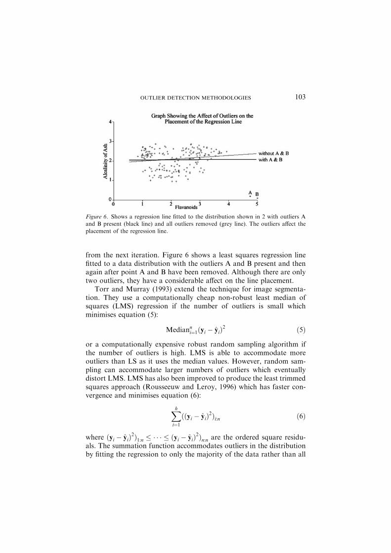
from the next iteration. Figure 6 shows a least squares regression linefitted to a data distribution with the outliers A and B present and thenagain after point A and B have been removed. Although there are onlytwo outliers, they have a considerable affect on the line placement.

Torr and Murray (1993) extend the technique for image segmenta-tion. They use a computationally cheap non-robust least median ofsquares (LMS) regression if the number of outliers is small whichminimises equation (5):

Medianni¼1ðyi � yiÞ2 ð5Þ

or a computationally expensive robust random sampling algorithm ifthe number of outliers is high. LMS is able to accommodate moreoutliers than LS as it uses the median values. However, random sam-pling can accommodate larger numbers of outliers which eventuallydistort LMS. LMS has also been improved to produce the least trimmedsquares approach (Rousseeuw and Leroy, 1996) which has faster con-vergence and minimises equation (6):

Xhi¼1

ððyi � yiÞ2Þi:n ð6Þ

where ðyi � yiÞ2Þ1:n � � � � � ðyi � yiÞ

2Þn:n are the ordered square residu-als. The summation function accommodates outliers in the distributionby fitting the regression to only the majority of the data rather than all

Figure 6. Shows a regression line fitted to the distribution shown in 2 with outliers Aand B present (black line) and all outliers removed (grey line). The outliers affect the

placement of the regression line.


of the data as in LMS. This region thus depicts normality and LTShighlights outliers as the points with large deviations from the majority.

MVE and convex peeling aim to compact the convex hull and cir-cumscribe the data with a decision boundary but are only applicable forlow dimensional data. Principal component analysis (PCA) (Parra et al.,1996; Faloutsos et al., 1997) in contrast, is suitable for higher dimen-sional data. It identifies correlated attributes in the data distribution andprojects the data onto this lower dimensional subspace. PCA is anunsupervised classifier but is linear and incapable of outperforming thecomplex non-linear class boundaries identified by the support vectormachine (see section 2.4) or neural methods described in section 3. PCAassumes that the subspaces determined by the principal components arecompact and this limits its applicability particularly for sparse distri-butions. However, it is an ideal pre-processor to select a subset ofattributes for methods which suffer the curse of dimensionality such asthe multi-layer perceptron in section 3, proximity-based techniques orsymplectic transformations described next. PCA identifies the principalcomponent of greatest variance as each component has an associatedeigenvalue whose magnitude corresponds to the variance of the pointsfrom the component vector. PCA retains the k principal componentswith greatest variance and discards all others to preserve maximuminformation and retain minimal redundancy.

Faloutsos et al. (1997) recommend retaining sufficient components sothe sum of the eigenvalues of all retained components is at least 85% ofthe sum of all eigenvalues. They use the principal components to predictattribute values in records by finding the intersection between the givenvalues for the record (i.e., excluding the omitted attribute) and theprincipal components. If the actual value for an attribute and the pre-dicted value differ then the record is flagged as an outlier. Parra et al.(1996) have developed a type-3 motor fault detector system which ap-plies PCA to the data and then applies a symplectic transformation tothe first few principal components. The symplectic transformation maybe used with non-linear data distributions. It maps the input data onto aGaussian distribution, conserving the volume and separating thetraining data (normal data) from the outliers. This double transfor-mation preserves information while removing redundancy, generates adensity estimation of the data set and thus allows a circular contour ofthe density to act as the decision boundary.

Baker et al. (1999) employ one of the hierarchical approaches de-tailed in this survey. The other hierarchical approaches are the decisiontree and cluster trees detailed in the machine learning section. Baker


uses a parametric model-based approach for novelty detection in a newsstory monitor. A hierarchy allows the domain knowledge to be repre-sented at various levels of abstraction so points can be compared fornovelty at a fine-grained or less specific level. The hierarchical statisticalalgorithm induces a topic hierarchy from the word distributions of newsstories using expectation maximisation (EM) to estimate the parametersettings followed by deterministic annealing (DA). DA constructs thehierarchy via maximum likelihood and information theory using adivisive clustering approach to split nodes into sub-nodes, starting froma single cluster, and build the hierarchy top–down. DA stochasticallydetermines the node to split. The system detects novelty when newnodes are added to the hierarchy that represent documents that do notbelong to any of the existing event clusters so new events are effectivelydescribed by their position in the hierarchy. When EM is used in con-junction with DA it avoids some of the initialisation dependence of EMbut at the cost of computational efficiency. DA can avoid local minimawhich EM is susceptible to but it may produce sub-optimal results.

2.3. Non-parametric methods

Many statistical methods described in this section have data-specificparameters ranging from the k values of k-NN and k-means to distancethresholds for the proximity-based approaches to complex modelparameters. Other techniques such as those based around convex hullsand regression and the PCA approaches assume the data follows aspecific model. These all require a priori data knowledge. Such infor-mation is often not available or is expensive to compute. Many data setssimply do not follow one specific distribution model and are oftenrandomly distributed. Hence, these approaches may be applicable for anoutlier detector where all data is accumulated beforehand and may bepre-processed to determine parameter settings or for data where thedistribution model is known. Non-parametric approaches, in contrastare more flexible and autonomous.

Dasgupta and Forrest (1996) introduce a non-parametric approachfor novelty detection in machinery operation. The authors recognisenovelty which contrasts to the other type 3 approaches we describe suchas k-means (Nairac et al., 1999) or the ART neural approach (Caudelland Newman, 1993) in section 3 which recognise or classify the normaldata space. The machinery operation produces a time-series of real-valued machinery measurements which Dasgupta and Forrest map ontobinary vectors using quantisation (binning). The binary vector (string)


effectively represents an encoding of the last n real-values from the timeseries. As the machinery is constantly monitored, new strings (binaryvector windows) are generated to represent the current operatingcharacteristics. Dasgupta and Forrest use a set of detectors where alldetectors fail to match any strings defining normality (where two stringsmatch if they are identical in a fixed number of contiguous positions (r)).If any detectors match a new string (a new time window of operatingcharacteristics) then a novelty has been detected. The value of r affectsthe performance of the algorithm and the value must be selected care-fully by empirical testing which inevitably slows processing. Eachindividual recogniser represents a subsection of the input distributionand compares the input. Dasgupta and Forrest’s approach wouldeffectively model Figure 5 by failing to match any point within thenormal boundary but would match any point from outside.

2.4. Semi-parametric methods

Semi-parametric methods apply local kernel models rather than a singleglobal distribution model. They aim to combine the speed and com-plexity growth advantage of parametric methods with the model flexi-bility of non-parametric methods. Kernel-based methods estimate thedensity distribution of the input space and identify outliers as lying inregions of low density. Roberts and Tarassenko (1995) and Bishop(1994) use Gaussian mixture models to learn a model of normal data byincrementally learning new exemplars. The GMM is represented byequation (7):

pðtjxÞ ¼XMj¼1

ajðxÞ/jðtjxÞ ð7Þ

whereM is the number of kernels (/), ajðxÞ the mixing coefficients, x theinput vector and t the target vector. Tarassenko and Roberts classifyEEG signatures to detect abnormal signals which represent medicalconditions such as epilepsy. In both approaches, each mixture repre-sents a kernel whose width is autonomously determined by the spread ofthe data. In Bishop’s approach the number of mixture models isdetermined using cross-validation. Tarassenko and Roberts’ techniqueadds new mixture models incrementally. If the mixture that best rep-resents the new exemplar is above a threshold distance, then the algo-rithm adds a new mixture. This distance threshold is determinedautonomously during system training. Once training is completed, the


final distance threshold represents the novelty threshold for new itemsto compare against. A Gaussian probability density function is definedby equation (8):

/jðtjxÞ ¼1

ð2pÞd2rdj ðxÞ

exp �kt� ljðxÞk2

2r2j ðxÞ

( )ð8Þ

where d is the dimensionality of the input space, r is the smoothingparameter, ljðxÞ represents the centre of the jth kernel and r2j ðxÞ is thevariance (width). This growing approach is somewhat analogous togrowing neural networks in section 3 as it adds a new mixture where it isnot modelling the data distribution well.

Roberts (1998) introduced extreme value theory which uses aGaussian mixture model to represent the data distribution for outlierdetection as outliers (extreme values) occur in the tails of the distribu-tions as points V, W, X, Y and Z in Figure 2 are extreme values. LeastSquares regression described earlier compares the outliers against thecorrelation of the data distribution whereas EVT compares themagainst a model of the distribution. EVT again uses EM to estimate thealgorithm’s parameter set. EVT examines the distribution tails andestimates the probability that a given instance is an extreme value in thedistribution model given by equation (9):

PðextremexÞ ¼ exp � exp � xm � lmrm

� �� ð9Þ

The approach is more principled than the proximity-based thresholdingtechniques discussed previously where a point is an outlier if it exceeds athreshold distance from the normal class as the EVT threshold is setusing a heuristic approach. EVT is ideal for novelty recognition whereabnormal samples are difficult or costly to obtain such as rare medicalcases or expensive machinery malfunctions. It is also not limited topreviously seen classes and is suitable for all three types of outlierdetection. A classifier, such as the multi-layer perceptron (section 3.1) ordecision trees (section 4), would attempt to place a new exemplar from apreviously unseen class in one of the classes it has previously learnedand would fail to detect the novelty.

The regression techniques and PCA are linear models which are toosimple for many practical applications. Tax et al. (1999) and DeCosteand Levine (2000) use support vector machines (SVMs) for type 2classification which use linear models to implement complex classboundaries. They project the input data onto higher dimensional kernels


using a kernel function in an attempt to find a hyper-plane that sepa-rates normal and abnormal data. Such a class-defining hyper-plane maynot be evident at the lower dimensions. The kernel functions range fromlinear dot product, polynomial non-linear used by DeCoste and Levine,a sigmoid kernel function which is equivalent to a multi-layer percep-tron see section 3.1. with no hidden layers and a Gaussian function as inequation (8) used in Tax et al. which is equivalent to a radial basisfunction neural network described in section 3.1. Support vectorsfunctions are positive in the dense regions of the data distribution andnegative in the sparsest regions of the distribution where the outliers lie.A support vector function is defined by equation (10):

SV ¼ signXnj¼1

ajLjKðxj; zÞ þ b

!ð10Þ

where K is the Kernel function, sign is a function returning þ1 if thedata is positive and �1 if the data is negative, Lj is the class label, b isthe bias, z the test input and xj the trained input. The data points thatdefine the class boundary of normality are the support vectors. Only thissmall set of support vectors need be stored often less than 10% of thetraining set so a large data set can effectively be stored using a smallnumber of exemplars.

Tax et al. (1999) use support vector novelty detection for machinecondition monitoring and medical classification. SVMs can induce aclassifier from a poorly balanced data set where the abnormal/normalexemplars are disproportional which is particularly true in medicaldomains where abnormal or in some case normal data is difficult andcostly to obtain. However, SVMs are computationally complex todetermine so heuristics have been devised to prevent this (DeCoste andLevine, 2000). DeCoste and Levine adapt the conventional SVM forspace instrument event detection by adapting the feature weights andthe cost of false positives as their data set is predominantly negative withfew positive instances of an event available for training.

3. Neural Networks

Neural network approaches are generally non-parametric and model-based, they generalise well to unseen patterns and are capable oflearning complex class boundaries. After training the neural networkforms a classifier. However, the entire data set has to be traversednumerous times to allow the network to settle and model the data


correctly. They also require both training and testing to fine tune thenetwork and determine threshold settings before they are ready forthe classification of new data. Many neural networks are susceptible tothe curse of dimensionality though less so than the statistical techniques.The neural networks attempt to fit a surface over the data and theremust be sufficient data density to discern the surface. Most neuralnetworks automatically reduce the input features to focus on the keyattributes. But nevertheless, they still benefit from feature selection orlower dimensionality data projections.

3.1. Supervised neural methods

Supervised neural networks use the classification of the data to drive thelearning process. The neural network uses the class to adjust the weightsand thresholds to ensure the network can correctly classify the input.The input data is effectively modelled by the whole network with eachpoint distributed across all nodes and the output representing theclassification. For example, the data in Figure 4 is represented by theweights and connections of the entire network.

Some supervised neural networks such as the multi-layer perceptroninterpolate well but perform poorly for extrapolation so cannot classifyunseen instances outside the bounds of the training set. Nairacet al. (1999) and Bishop (1994) both exploit this for identifying novel-ties. Nairac identifies novelties in time-series data for fault diagnosis invibration signatures of aircraft engines and Bishop monitors processessuch as oil pipeline flows. The MLP is a feed forward network. Bishopand Nairac use a MLP with a single hidden layer. This allows thenetwork to detect arbitrarily complex class boundaries. The nodes in thefirst layer define convex hulls analogous to the convex hull statisticalmethods discussed in the previous section. These then form the inputsfor the second layer units which combine hulls to form complex classes.Bishop notes that the non-linearity offered by the MLP classifier pro-vides a performance improvement compared to a linear technique. It istrained by minimising the square error between the actual value and theMLP output value given by equation (11):

Error ¼Xmj¼1

Z½yjðx;wÞ � htjjxi�2pðxÞdx

þXmj¼1

Zfht2j jxi � htjjxi2gpðxÞdx ð11Þ


from Bishop (1994) where tj is the target class, yj is the actual class, pðxÞis the unconditional probability density which may be estimated by, forexample, Parzen windows (Bishop, 1994) (discussed in section 5) andyjðx;wÞ is the function mapping. Provided the function mapping isflexible, if the network has sufficient hidden units, then the minimumoccurs when yjðx;wÞ ¼ phtjjxi. The outputs of the network are theregression of the target data conditioned with the input vector. The aimis thus to approximate the regression by minimising the sum-of-squareserror using a finite training set. The approximation is highest where thedensity of pðxÞ is highest as this is where the error function penalises thenetwork mapping if it differs from the regression. Where the density islow there is little penalisation. Bishop assumes that the MLP ‘knows’the full scope of normality after training so the density pðxÞ is high, thenetwork is interpolating and confidence is high (where confidence isgiven by equation (12):

ryðxÞ ¼ fpðxÞg12 ð12Þ

If a new input lies outside the trained distribution where the den-sity pðxÞ is low and the network is extrapolating, the MLP willnot recognise it and the confidence is low. Nairac uses the MLPto predict the expected next value based on the previous n values.This assumes that the next value is dependent only on the previous nvalues and ignores extraneous factors. If the actual value differsmarkedly from the predicted value then the system alerts the humanmonitoring it.

Japkowicz et al. (1995) use an auto-associative neural network fortype 3 novelty recognition. The auto associator network is also a feed-forward perceptron-based network which uses supervised learning.Auto associators decrease the number of hidden nodes during networktraining to induce a bottleneck. The bottleneck reduces redundancies byfocusing on the key attributes while maintaining and separating theessential input information and is analogous to principal componentanalysis. Japkowicz trains the auto-associator with normal data only.After training, the output nodes recreate the new exemplars applied tothe network as inputs. The network will successfully recreate normaldata but will generate a high re-creation error for novel data. Japkowiczcounts the number of outputs different from the input. If this valueexceeds a pre-specified threshold then the input is recognised as novel.Japkowicz sets the threshold at a level that minimises both false positiveand false negative classifications. Taylor and Addison (2000) demon-strated that auto-associative neural networks were more accurate than


SOMs or Parzen windows for novelty detection. However, auto-asso-ciators suffer slow training as with the MLP and have various data-specific parameters which must be set through empirical testing andrefinement.

Hopfield networks are also auto-associative and perform supervisedlearning. However, all node weights are þ1 or �1 and it is fully con-nected with no bottleneck. Hopfield nets are computationally efficientand their performance is evident when a large number of patterns isstored and the input vectors are high dimensional. Crook and Hayes(1995) use a Hopfield network for type 3 novelty detection in mobilerobots. The authors train the Hopfield network with pre-classifiednormal exemplars. The input pattern is applied to all nodes simulta-neously unlike the MLP where the input ripples through the layers ofthe network. The output is fed back into the network as input to allnodes. Retrieval from a Hopfield network requires several networkcycles while node weights update and to allow the network to settle andconverge towards the ‘best compromise solution’ (Beale and Jackson,1990). However, the energy calculation requires only the calculation ofthe sum of the weights see equation (13):

Energy ¼ � 1

2

XNi¼1

XNj¼1

xixjwij ð13Þ

where N is the number of neurons and thus has a fixed execution timeregardless of the number of input patterns stored providing a compu-tationally efficient retrieval mechanism. If the energy is above athreshold value calculated from the distribution model and the numberof patterns stored then Crook and Hayes classify the input as novel.During empirical testing, the Hopfield network trained faster thanMarsland’s HSOM but the HSOM discerned finer-grained image detailsthan the Hopfield network.

The MLP uses hyper-planes to classify the data. In contrast, thesupervised radial basis function (RBF) neural network in Bishop (1994)and Brotherton et al. (1998) uses hyper-ellipsoids defined by equation(14) for k dimensional inputs:

sk ¼Xmj¼1

wjk/ðkx� yjkÞ ð14Þ

where wjk is the weight from the kernel to the output, / is a Gaussianfunction (see equation (8)) and k � � � k the Euclidean distance. RBF is alinear combination of basis functions similar to a Gaussian mixture


model and guaranteed to produce a solution as hyper-ellipsoids guar-antee linear separability (Bishop, 1995). Training the network is muchfaster than an MLP and requires two stages: the first stage clusters theinput data into the hidden layer nodes using vector quantisation. TheRBF derives the radius of the kernel from the data as with the Gaussianmixture model approach (see equation (8)) using the kernel centre andvariance. The second training stage weights the hidden node outputsusing least mean squares weighting to produce the required outputclassification from the network.

Brotherton et al. (1998) revise the network topology and vectorquantisation so there is a group of hidden nodes exclusively assigned foreach class with a separate vector quantisation metric for each class. Thismeans that the groups of hidden nodes represent distinct categoriesunlike a conventional RBF where weight combinations of all hiddennodes represent the categories. The output from each group of nodescorresponds to the probability that the input vector belongs to the classrepresented by the group. Brotherton uses the adapted RBF for type 3novelty recognition in electromagnetic data or machine vibrationanalysis. Brotherton’s adaptation creates an incremental RBF. Newnodes can be added to represent new classes just as new mixtures areadded to Roberts and Tarassenko’s (1995) adaptive mixture model ornew category nodes are added to evolutionary neural networks.

3.2. Unsupervised neural methods

Supervised networks require a pre-classified data set to permit learning.If this pre-classification is unavailable then an unsupervised neuralnetwork is desirable. Unsupervised neural networks contain nodeswhich compete to represent portions of the data set. As with perceptron-based neural networks, decision trees or k-means, they require a trainingdata set to allow the network to learn. They autonomously cluster theinput vectors through node placement to allow the underlying datadistribution to be modelled and the normal/abnormal classes differen-tiated. They assume that related vectors have common feature valuesand rely on identifying these features and their values to topologicallymodel the data distribution.

Self organising maps, Kohonen (1997) are competitive, unsupervisedneural networks. SOMs perform vector quantisation and non-linearmapping to project the data distribution onto a lower dimensional gridnetwork whose topology needs to be pre-specified by the user. Each nodein the grid has an associated weight vector analogous to the mean vector


representing each cluster in a k-means system. The network learns byiteratively reading each input from the training data set, finding the bestmatching unit, updating the winner’s weight vector to reflect the newmatch like k-means. However, the SOM also updates the neighbouringnodes around the winner unlike k-means. This clusters the network intoregions of similarity. The radius of the local neighbourhood shrinksduring training in the standard SOM and training terminates when theradius of the neighbourhood reaches its minimum permissible value.Conversely, Ypma and Duin (1997) enlarges the final neighbourhood toincrease the SOMs ‘stiffness’ by providing broader nodes to prevent overfitting. After training, the network has evolved to represent the normalclass. In Figure 5, the SOM nodes would model the normal class, dis-tributed according to the probability density of the data distribution.

During novelty recognition, the unseen exemplar forms the input tothe network and the SOM algorithm determines the best matching unit.In Saunders and Gero (2001a) and Vesanto et al. (1998), if the vectordistance or quantisation error between the best matching unit (bmu)and new exemplar exceeds some pre-specified threshold (d) then theexemplar is classified as novel. Equation (15) gives the minimum vectordistance for the bmu and compares this to the threshold.

minXn�1

i¼0

ðxiðtÞ � wijðtÞÞ2 !

> d ð15Þ

For example, if the SOM nodes modelled Figure 5 (the normal classfrom Figure 2), the points V, W, X, Y and Z from Figure 2 would all bedistant from their respective best matching units and would exceed d soV, W, X, Y and Z would be identified as novel. This is analogous to ak-means approach (section 2.1); the SOM equates to a k-means clus-tering with k equivalent to the number of SOM nodes. However, SOMsuse a user-specified global distance threshold whereas k-means auton-omously determines the boundary during training allowing local settingof the radius of normality as defined by each cluster. This distancematch can be over simplistic and requires the selection of a suitabledistance threshold so other approaches examine the response of allnodes in the grid. Himberg et al. (2001) look at the quantisation errorfrom the input to all nodes, given by equation (16):

gðx;miÞ ¼1

1þ kx�mika

� �2 ð16Þ


where a is the average distance between each training data and its bmumi. The scaling factor compares the distance between x and its bmu mi

against the overall average accuracy of the map nodes during training.Ypma and Duin (1997) uses a further advancement for mechanical faultdetection. They recommend an approach unifying normalised distancemeasure for 2 and 3 nearest neighbours rather than a single nearestneighbour of Saunders and Gero and Vesanto and normalised mean-square error of mapping.

Saunders and Gero (2001b) and Marsland’s (2001) systems usean extended SOM, the Habituating SOMs (HSOMs) where everynode is connected to an output neuron through habituating syn-apses which perform inverse Hebbian learning by reducing their con-nection strength through frequency of activation. The SOM forms anovelty detector where the novelty of the input is proportional to thestrength of the output thus simplifying novelty detection compared to aconventional SOM as the output node indicates novelty, there is norequirement for identifying best matching units or complex quantisationerror calculations. The HSOM requires minimal computational re-sources and is capable of operating and performing novelty detectionembedded in a robot (Marsland, 2001). It also trains quickly andaccurately. However, HSOMs are susceptible to saturation where anyinput will produce a low strength output as the HSOM cannot addnew nodes and the number of classes (groups of inputs mapping toparticular nodes) in the input distribution is equal to or greater than thenumber of nodes. If the number of classes is known in advance, then asuitable number of nodes can be pre-selected but for many outlierdetection problems, particularly on-line learning problems, this infor-mation may not be available.

Evolutionary neural network growth is analogous to Roberts andTarassenko’s (1995) approach of adding new Gaussian mixtures when anew datum does not fit any of the existing mixtures. Marsland (2001)introduces the grow when required (GWR) evolutionary neural networkfor type 3 novel feature detection in a mobile inspection robot (robotneotaxis). It is suited to on-line learning and novelty recognition as thenetwork can adapt and accurately model a dynamic data distribution.The growing neural network connects the best matching node and thesecond best match and adds new nodes when the response of the bestmatching node for an input vector is below some threshold value. TheGWR network grows rapidly during the first phase of training but onceall inputs have been processed (assuming a static training set), then thenumber of nodes stabilises and the network accurately represents the


data distribution. As with the SOM, the GWR would learn the normalclass in Figure 5 and the points V, W, X, Y and Z from Figure 2 wouldall then be distant from their respective best matching units which are allwithin the normal class.

Caudell and Newman (1993) introduce a type 3 recogniser for time-series monitoring based on the adaptive resonance theory (ART)(Carpenter and Grossberg, 1987) incremental unsupervised neural net-work. The network is plastic while learning, then stable while classifyingbut can return to plasticity to learn again making them ideal for time-series monitoring. The ART network trains by taking a new instancevector as input, matching this against the classes currently covered bythe network and if the new data does not match an existing class givenby equation (17): Pn

i¼1 wijðtÞxiPni¼1 xi

> q ð17Þ

where n is the input dimensionality and q is a user-specified parameter(vigilance threshold) then it creates a new class by adding a new nodewithin the network to accommodate it. Caudell and Newman monitorthe current ART classes and when the network adds a new class thisindicates a change in the time series. GWR grows similarly but GWR istopology preserving with neighbourhoods of node representing similarinputs whereas ART simply aims to cover the entire input space uni-formly. By only adding a new node if the existing mapping is insufficientand leaving the network unchanged otherwise, the ART network doesnot suffer from over-fitting which is a problem for MLPs and decisiontrees. The training phase also requires only a single pass through theinput vectors unlike the previously described neural networks whichrequire repeated presentation of the input vectors to train. Duringempirical evaluation, Marsland (2001) noted that the performance ofthe ART network was extremely disappointing for robot neotaxis. TheART network is not robust and thus susceptible to noise. If the vigilanceparameter is set too high the network becomes too sensitive and addsnew classes too often.

4. Machine Learning

Much outlier detection has only focused on continuous real-valued dataattributes there has been little focus on categorical data. Most statisticaland neural approaches require cardinal or at the least ordinal data to


allow vector distances to be calculated and have no mechanism forprocessing categorical data with no implicit ordering. John (1995) andSkalak and Rissland (1990) use a C4.5 decision tree to detect outliers incategorical data and thus identify errors and unexpected entries in da-tabases. Decision trees do not require any prior knowledge of the dataunlike many statistical methods or neural methods that requireparameters or distribution models derived from the data set. Con-versely, decision trees have simple class boundaries compared with thecomplex class boundaries yielded by neural or SVM approaches.Decision trees are robust, do not suffer the curse of dimensionality asthey focus on the salient attributes, and work well on noisy data. C4.5 isscalable and can accommodate large data sets and high dimensionaldata with acceptable running times as they only require a single trainingphase. C4.5 is suited to type 2 classifier systems but not to noveltyrecognisers which require algorithms such as k-means which can definea boundary of normality and recognise whether new data lies inside oroutside the boundary. However, decision trees are dependent on thecoverage of the training data as with many classifiers. They are alsosusceptible to over fitting where they do not generalise well to com-pletely novel instances which is also a problem for many neural networkmethods. There are two solutions to over-fitting: pre-selection of recordsor pruning.

Skalak and Rissland (1990) pre-select cases using the taxonomy froma case-based retrieval algorithm to pinpoint the ‘most-on-point-cases’and exclude outliers. They then train a decision tree with this pre-selected subset of normal cases. Many authors recommend pruningsuperfluous nodes to improve the generalisation capabilities and preventover-fitting. John (1995) exploits this tactic and uses repeated pruningand retraining of the decision tree to derive the optimal tree represen-tation until no further pruning is possible. The pruned nodes representthe outliers in the database and are systematically removed until onlythe majority of normal points are left.

Arning et al. (1996) also uses pruning but in a set-based machine-learning approach. It processes categorical data and can identify out-liers where there are errors in any combination of variables. Arningidentifies the subset of the data to discard that produces the greatestreduction in complexity relative to the amount of data discarded. Heexamines the data as a sequence and uses a set-based dissimilarityfunction to determine how dissimilar the new exemplar is compared tothe set of exemplars already examined. A large dissimilarity indicates apotential outlier. The algorithm can run in linear time though this relies


on prior knowledge of the data but even without prior knowledge, it isstill feasible to process large data mining data sets with the approach.However, even the authors note that it is not possible to have a uni-versally applicable dissimilarity function as the function accuracy is datadependent. This pruning is analogous to the statistical techniques (seesection 2.2) of convex peeling or Torr and Murray’s approach ofshedding points and re-fitting the regression line to the remaining data.

Another machine learning technique exploited for outlier detection isrule-based systems which are very similar to decision trees as they bothtest a series of conditions (antecedents) before producing a conclusion(class). In fact rules may be generated directly from the paths in thedecision tree. Rule-based systems are more flexible and incremental thandecision trees as new rules may be added or rules amended withoutdisturbing the existing rules. A decision tree may require the generationof a complete new tree. Fawcett and Provost (1999) describe their DC-1activity monitoring system for detecting fraudulent activity or newsstory monitoring. The rule-based module may be either a classifierlearning classification rules from both normal and abnormal trainingdata or a recogniser trained on normal data only and learning rules topinpoint changes that identify fraudulent activity. The learned rulescreate profiling monitors for each rule modelling the behaviour of asingle entity, such as a phone account. When the activity of the entitydeviates from the expected, the output from the profiling monitor re-flects this. All profiling monitors relating to a single entity feed into adetector which combines the inputs and generates an alarm if thedeviation exceeds a threshold. This approach detects deviations in se-quences compared to Nairac’s time-series approach which uses one-stepahead prediction to compare the expected next value in a sequence withthe actual value measured. There is no prediction in activity monitoringall comparisons use actual measured values.

Lane and Brodley (1997a, b) introduced a similar approach foractivity monitoring using similarity-based matching. The system storesand records the activities of users on a computer system as sequences.The system uses similarity-based matching to compare command se-quences issued by users against the stored sequences. Due to the asyn-chronous nature of human-computer interaction, a new fraudulentcommand sequence is unlikely to exactly match a previously storedsequence. The matching metric must allow for the interpolation of gapsand non-matching sub-sequences reflecting, for example, the user col-lecting an incoming e-mail. Lane and Brodley take their cue from Mi-chalski’s (Dietterich and Michalski, 1985) sequential data modelling


techniques and generate a validity analysis for each step in the com-mand sequence entered. They incorporate adjacency into their similaritymetric. If the similarity value is between a lower and upper boundthreshold then the current sequence up to and including the currentcommand is not anomalous.

Data mining algorithms such as BIRCH (Zhang et al., 1996) andDBSCAN (Ester et al., 1996) are robust and as such tolerant to outliersbut were specifically optimised for clustering large data sets. They arebased around tree structured indices and cluster hierarchies. Bothtechniques are capable of identifying outliers but cannot provide a de-gree of novelty score. BIRCH (Zhang et al., 1996) uses local clusteringand data compression and has O(n) running time. BIRCH can operateincrementally, clustering data as and when it becomes available. How-ever, it is limited to numerical data and is dependent on the order ofpresentation of the data set. It uses a specialised balanced tree structurecalled a CF-tree which is designed for large, high dimensional data setsand induces a good quality clustering from only a single pass throughthe data set which can optionally be improved by further passes. It canonly store a limited number of records in each tree node and this canlead to an artificial cluster topology.

DBSCAN (Ester et al., 1996) is density-based with Oðn log nÞ run-ning time and generates an R*-tree to cluster the data and identify the knearest neighbours. It can identify clusters of arbitrary shape like theGaussian mixture model described earlier. DBSCAN has two user-specified parameters which determine the density of the data in the treebut it autonomously determines the number of clusters unlike forexample the k-means algorithm. One parameter, the number of neigh-bours is generally set to 4 but the other parameter (the neighbourhooddistance) requires Oðn log nÞ time to calculate. The pre-initialisationstep for DBSCAN calculates the distance between a point and its fourthnearest neighbours, plots the distance graph and then requires the userto find a valley in the distance plot. The user must identify where thevalley begins from the graph profile and set the parameter accordingly.

5. Hybrid Systems

The most recent development in outlier detection technology is hybridsystems. The hybrid systems discussed in this section incorporatealgorithms from at least two of the preceding sections (statistical, neuralor machine learning methods). Hybridisation is used variously to


overcome deficiencies with one particular classification algorithm, toexploit the advantages of multiple approaches while overcoming theirweaknesses or using a meta-classifier to reconcile the outputs frommultiple classifiers to handle all situations. We describe approacheswhere an additional algorithm is incorporated to overcome weaknesseswith the primary algorithm next.

The MLP described in section 3 interpolates well but cannotextrapolate to unseen instances. Therefore, Bishop (1994) augments hisMLP with a Parzen window novelty recogniser. The MLP classifies newitems similar to those already seen with high confidence. The Parzenwindow provides an estimate of the probability density to induce aconfidence estimate. Any completely novel instances will lie in a lowdensity and the MLP prediction confidence will be low. Parzen windowsare kernel-based algorithms which use various kernel functions to rep-resent the data. Bishop uses one Gaussian kernel (as defined by equation(8)) per input vector with the kernel centred on the attribute values ofthe vector. The Parzen window method can provide a hard boundaryfor outlier detection by classifying new exemplar as normal if they be-long to a kernel and an outlier otherwise. It can also provide a softboundary by calculating the probability that the new exemplar belongsto a Gaussian kernel. Nairac et al. (1999) similarly incorporate ak-means module with the MLP module in an aircraft engine fault diag-nosis system. The k-means module partitions the data and models graphshape normality. It can detect anomalies in the overall vibration shape ofnew signatures and the MLP detects transitions within the vibrationgraphs through one-step ahead prediction described in section 3.

Smyth (1994) stabilises the output from an MLP to monitor spaceprobe data for fault detection using a hidden Markov model (HMM) asthe MLP is susceptible to rapid prediction changes many of which areextraneous. The approach uses time-series data, a snapshot of the spaceprobe transmitted periodically with equal intervals between transmis-sions. The feed-forward MLP trained using back propagation aims tomodel the probe and predicts the next state of the probe. However, theMLP has a tendency to switch between states at an artificially high rateso Smyth uses a HMM to correlate the state estimations and smooth theoutputs producing a predictor with high accuracy. Hollmen and Tresp(1999) incorporate hierarchical HMMs with EM which helps determinethe parameters for time series analysis in the task of cell-phone frauddetection. The authors use the HMM to predict one-step ahead valuesfor a fraud variable in the time series given the current and previousstates of a user’s account and the EM algorithm is used to provide


optimal parameter settings for the HMM to enable accurate one-stepahead prediction.

Hickinbotham and Austin (2000) introduced a strain gauge faultdetection system to detect gauges which are not reading correctly. Thesystem assimilates Gaussian basis function networks (GBFN) andprincipal components. The technique produces a frequency of occur-rence matrix (FOOM) from data taken from aircraft strain gaugesoperating under normal conditions. The FOOM represents the normalconditions expected during a flight with readings weighted according totheir likelihood of occurrence. The approach extracts two unlikelinessfeatures and two principal components from the FOOM and feeds theminto a series of GBFN, each trained with different parameter settings.The system selects the GBFN with highest classification accuracy for thedata and uses this to classify new FOOMs by thresholding for novelty.A high novelty reading indicates a strain gauge error. Hollier andAustin (2002) have incorporated a further component into the straingauge system to detect another form of strain gauge error not coveredby the previous approach. They incorporate auxiliary data comprising avector of accelerations encountered during a flight. Hollier and Austinfind the maximally correlated components between the FOOM and themean and first principal component of the auxiliary data. By estab-lishing a relationship between the auxiliary data and normal FOOMs,they can detect corrupted FOOMs when the relationship breaks down.

Authors are beginning to examine the possibilities of ensembleclassifiers where a number of different classification algorithms are usedand the results from each classifier amalgamated using a suitable metric.From the preceding discussion, it is apparent that all classifiers havediffering strengths and weaknesses so a combined approach can exploitthe strengths of each classifier while mitigating their weaknesses.

The JAM system (Java agents for meta-learning) being developed atColumbia University (Stolfo et al., 1997) incorporates five machine-learning techniques into a single modular architecture. JAM uses meta-learning to assimilate the results from the various modules and produce asingle system output. JAM modules are based on the ID3 decision tree(Quinlan, 1986), its successors CART (Breiman et al., 1984) and C4.5(Quinlan, 1993), Ripper (a rule based learner; Cohen, 1995) and a naiveBayes classifier. In experiments, Prodromidis and Stolfo (1998) demon-strated that these classifiers were complimentary, each performingwell onsomedata sets and comparatively poorly onother data sets. By identifyingwhich approaches excel onwhichdata sets andunderwhich conditions themeta-learner can assess the degree of accuracy and confidence for the


outputs from the various classifiers and select the appropriate techniquefor the data. Ensemble classifiers also permit sub-division of the trainingdata with individual classifier modules trained on subsets of the data. Byusingmultiple datamodels, JAMmitigates for any loss of accuracy in anyone model due to data subdivision. It allows parallel training and classi-fication with each module classifying a new instance in parallel and themeta-learner metric assimilating the results.

Brodley and Friedl (1996) also use an ensemble approach for iden-tifying misclassified instances in a training set of pixels from satelliteimages of land where each pixel needs to be classified as for example,grassland, woodland, etc. They use three classifiers: a decision tree, anearest neighbour and a linear machine. The system combines theoutputs from the three classifiers using consensus voting. Consensusvoting is a more conservative approach than the widely used majorityvoting. In consensus voting, the system only eliminates an instance fromthe data set if all three classifiers identify it as an outlier whereas amajority voting system eliminates an instance if the majority of classi-fiers identify it as an outlier. Consensus voting favours false negativesover false positives with respect to identifying outliers. The three clas-sifiers each use a different distribution model so if all three agree that apoint is an outlier then the user can be confident about the decision.

Combining multiple classifiers must be done judiciously. An ensem-ble should obey Occam’s Razor, it should be as simple as possible withminimal redundancy, as superfluous modules waste resources, increasecomplexity and slow processing. Paradoxically, identifying the bestcombination of classifiers is a combinatorial problem.

6. Conclusions

There is no single universally applicable or generic outlier detectionapproach. From the previous descriptions, authors have applied a widevariety of techniques covering the full gamut of statistical, neural andmachine learning techniques. We have tried to provide a broad sampleof current techniques but obviously, we are unable to describe all ap-proaches in a single paper. We hope to have provided the reader with afeel of the diversity and multiplicity of techniques available.

In outlier detection, the developer should select an algorithm that issuitable for their data set in terms of the correct distribution model, thecorrect attribute types, the scalability, the speed, any incremental capa-bilities to allow new exemplars to be stored and the modelling accuracy.


The developer should also consider which of the three fundamentalapproaches is suitable for their problem, a clustering approach, a clas-sification approach or a novelty approach. This will depend on: the datatype, whether the data is pre-labelled, the ground truth of the labelling(i.e., whether any novel records will be mislabelled as normal), how theywish to detect outliers and how they wish to handle them.

How the developers wish to handle outliers is very important, whetherthey wish to expunge them from future processing in a diagnostic clus-tering or a recognition systemor retain themwith an appropriate label in aaccommodating clustering or a classification system. Developers shouldalso consider whether they wish to simply classify a new exemplar as anoutlier or notorwhether theywish toapply a scale of ‘outlierness’ suchas apercentage probability that the particular point is an outlier. The devel-oper should carefully consider anypre-processing theywill performon thedata such as feature extraction or prototyping to reduce the storageoverhead of the data. Alternatively they can select an approach such as k-meansor support vectormachines that storeonly aminimal data setwhicheffectively covers the data distribution through a small subset of seminalexemplars. Francis et al. (1999) showed equivalent classification accuracywhen the data set of a novelty detection system based on neural networkapproaches was pre-processed with feature extraction compared to theclassification accuracy with that of the novelty detector trained using thefull range of attributes. The authors used linear regression to combinemultiple attributes into single dependent attributes.

Acknowledgements

We wish to thank the reviewers for their insightful comments that al-lowed us to improve this paper. This work was supported by EPSRCGrant No. GR/R55191/01.

Note

There are statistical models for symbolic data (such as log-linear models) but these are not

generally used for outlier analysis.

References

Aggarwal, C. C. & Yu, P. S. (2001). Outlier Detection for High Dimensional Data.

Proceedings of the ACM SIGMOD Conference 2001.


Aha, D. W. & Bankert, R. B. (1994). Feature Selection for Case-Based Classification ofCloud Types: An Empirical Comparison. Proceedings of the AAAI-94 Workshop on

Case-Based Reasoning.Allan, J., Carbonell, J., Doddington, G., Yamron, J. & Yang, Y. (1998). Topic

Detection and Tracking Pilot Study: Final Report. Proceedings of the DARPA

Broadcast News Transcription and Understanding Workshop.Arning, A., Agrawal, R. & Raghavan, P. (1996). A Linear Method for Deviation

Detection in Large Databases. Proceedings of the ACM SIGKDD InternationalConference on Knowledge Discovery and Data Mining, 164–169.

Baker, L. D., Hofmann, T., McCallum, A. K. & Yang, Y. (1999). A HierarchicalProbabilistic Model for Novelty Detection in Text. NIPS’99, Unpublished manu-script.

Barnett, V. & Lewis, T. (1994). Outliers in Statistical Data, 3rd edn. John Wiley & Sons.Beale, R. & Jackson, T. (1990). Neural Computing: An Introduction. Bristol, UK and

Philadelphia, PA: Institute of Physics Publishing.

Bishop, C. M. (1994). Novelty detection & Neural Network validation. Proceedings ofthe IEE Conference on Vision, Image and Signal Processing, 217–222.

Bishop, C. M. (1995). Neural Networks for Pattern Recognition. Oxford University

Press.Blake, C. L. & Merz, C. J. (1998). UCI Repository of Machine Learning Databases,

http://www.ics.uci.edu/mlearn/MLRepository.html, University of California, Ir-vine, Department of Information and Computer Sciences.

Bolton, R. J. & Hand, D. J. (2001). Unsupervised Profiling Methods for FraudDetection. Credit Scoring and Credit Control VII, Edinburgh, UK, 5–7September.

Bradley, P. S., Fayyad, U. M. & Mangasarian, O. L. (1999). Mathematical Program-ming for Data Mining: Formulations and Challenges. INFORMS Journal onComputing 11(3): 217–238.

Breiman, L., Friedman, J., Olshen, R. & Stone, C. (1984). Classification and RegressionTrees. Belmont, CA: Wadsworth International Group.

Brodley, C. E. & Friedl, M. A. (1996). Identifying and Eliminating Mislabeled TrainingInstances. Proceedings of the 13th National Conference on Artificial Intelligence, 799–

805, AAAI Press.Brotherton, T., Johnson, T. & Chadderdon, G. (1998). Classification and Novelty

Detection using Linear Models and a Class Dependent – Elliptical Bassi Function

Neural Network. Proceedings of the International conference on neural networks.Anchorage, Alaska.

Byers, S. & Raftery, A. E. (1998). Nearest Neighbor Clutter Removal for Estimating

Features in Spatial Point Processes. Journal of the American Statistical Association93(442): 577–584.

Carpenter, G. & Grossberg, S. (1987). ‘A Massively Parallel Architecture for a Self-

Organizing Neural Pattern Recognition Machine’. Computer Vision, Graphics, andImage Processing 37: 54–115.

Caudell, T. P. & Newman, D. S. (1993). An Adaptive Resonance Architecture to DefineNormality and Detect Novelties in Time Series and Databases. IEEE World Con-

gress on Neural Networks, Portland, Oregon. 166–176.Cohen, W. W. (1995). Fast Effective Rule Induction. International Conference on Ma-

chine Learning, 115–123.


Crook, P. & Hayes, G. (1995). A Robot Implementation of a Biologically InspiredMethod for Novelty Detection. Proceedings of TIMR-2001, Towards Intelligent

Mobile Robots Manchester.Dasgupta, D. & Forrest, S. (1996). Novelty Detection in Time Series Data Using Ideas

from Immunology. Proceedings of the Fifth International Conference on Intelligent

Systems.Datta, P. & Kibler, D. (1995). Learning prototypical concept descriptions. Proceedings

of the 12th International Conference on Machine Learning, 158–166, Morgan Ka-ufmann.

DeCoste, D. & Levine, M. B. (2000). Automated Event Detection in Space Instruments:A Case Study Using IPEX-2 Data and Support Vector Machines. Proceedings of theSPIE Conference on Astronomical Telescopes and Space Instrumentation.

Dietterich, T. G. & Michalski, R. S. (1986). Learning to Predict Sequences. In Mi-chalski, Carbonell & Mitchell (eds.) Machine Learning: An Artificial IntelligenceApproach San Mateo, CA: Morgan Kaufmann.

Ester, M., Kriegel, H. -P. & Xu, X. (1996). A Density-Based Algorithm for DiscoveringClusters in Large Spatial Databases with Noise. Proceedings of the Second Inter-national Conference on Knowledge Discovery and Data Mining, Portland, Oregon,

226–231. AAAI Press.Faloutsos, C., Korn, F., Labrinidis, A., Kotidis, Y., Kaplunovich, A. & Perkovic, D.

(1997). Quantifiable Data Mining Using Principal Component Analysis. TechnicalReport CS-TR-3754, Institute for Systems Research, University of Maryland,

College Park, MD.Fawcett, T. & Provost, F. J. (1999). Activity Monitoring: Noticing Interesting Changes

in Behavior. Proceedings of the 5th ACM SIGKDD International Conference on

Knowledge Discovery and Data Mining, 53–62.Francis, J., Addison, D., Wermter, S. & MacIntyre, J. (1999). Effectiveness of Feature

Extraction in Neural Network Architectures for Novelty Detection. Proceedings of

the ICANN Conference.Grubbs, F. E. (1969). Procedures for Detecting Outlying Observations in Samples.

Technometrics 11: 1–21.Hickinbotham, S. & Austin, J. (2000). Novelty Detection in Airframe Strain Data.

Proceedings of 15th International Conference on Pattern Recognition, Barcelona,536–539.

Himberg, J., Jussi, A., Alhoniemi, E., Vesanto, J. & Simula, O. (2001). The Self-

Organizing Map as a Tool in Knowledge Engineering, In Pattern Recognition inSoft Computing Paradigm, 38–65. Soft Computing. World ScientificPublishing.

Hollier, G. & Austin, J. (2002). Novelty Detection for Strain-Gauge Degradation UsingMaximally Correlated Components. Proceedings of the European Symposium onArtificial Neural Networks, ESANN’2002, Bruges, 257–262.

Hollmen, J. & Tresp, V. (1999). Call-based Fraud Detection in Mobile CommunicationNetworks using a Hierarchical Regime-Switching Model. Advances in NeuralInformation Processing Systems – Proceedings of the 1998 Conference (NIPS’11),889–895, MIT Press.

Japkowicz, N., Myers, C. & Gluck M. A. (1995). A Novelty Detection Approach toClassification. Proceedings of the 14th International Conference on Artificial Intelli-gence (IJCAI-95), 518–523.


John, G. H. (1995). Robust Decision Trees: Removing Outliers from Databases. Pro-ceedings of the First International Conference on Knowledge Discovery and Data

Mining, 174–179. Menlo Park, CA: AAAI Press.Knorr, E. M. & Ng, R. T. (1998). Algorithms for Mining Distance-Based Outliers in

Large Datasets. Proceedings of the VLDB Conference, 392–403, New York, USA.

Kohonen, T. (1997). Self-Organizing Maps, Vol. 2. Springer-Verlag, Heidelberg.Lane, T. & Brodley, C. E. (1997a). Applications of Machine Learning to Anomaly

Detection. In Adey, R.A., Rzevski, G, and Teti, T. (eds.) Applications of ArtificialIntelligence in Engineering X11, 113–14, Southampton, UK: Comput. Mech. Pub-

lications.Lane, T. & Brodley, C. E. (1997b). Sequence matching and learning in anomaly

detection for computer security. AAAI Workshop: AI Approaches to Fraud Detection

and Risk Management, 43–49. AAAI Press.Laurikkala, J., Juhola, M. & Kentala, E. (2000). Informal Identification of Outliers in

Medical Data. Fifth International Workshop on Intelligent Data Analysis in Medicine

and Pharmacology IDAMAP-2000 Berlin, 22 August. Organized as a workshop of the14th European Conference on Artificial Intelligence ECAI-2000.

Marsland, S. (2001). On-Line Novelty Detection Through Self-Organisation, with

Application to Inspection Robotics. Ph.D. Thesis, Faculty of Science and Engi-neering, University of Manchester, UK.

Nairac, A., Townsend, N., Carr, R., King, S., Cowley, P. & Tarassenko, L. (1999). ASystem for the Analysis of Jet System Vibration Data. Integrated ComputerAided

Engineering 6(1): 53–65.Ng, R. T. & Han, J. (1994). Efficient and Effective Clustering Methods for Spatial Data

Mining. Proceedings of the 20th International Conference on Very Large Data Bases,

September 12–15, 1994, Santiago, Chile, 144–155. Morgan Kaufmann Publishers.Parra, L., Deco, G. & Miesbach S. (1996). Statistical Independence and Novelty

Detection with Information Preserving Nonlinear Maps. Neural Computation 8 (2):

260–269.Prodromidis, A. L. & Stolfo, S. J. (1998). Mining Databases with Different Schemas:

Integrating Incompatible Classifiers. Proceedings of the ACM SIGKDD InternationalConference on Knowledge Discovery and Data Mining, 314–318.

Quinlan, J. R. (1986). Induction of Decision Trees. Machine Learning 1(1): 81–106.Quinlan, J. R. (1993). C4.5: Programs for Machine Learning. Morgan Kaufmann.Ramaswamy, S., Rastogi, R. & Shim, K. (2000). Efficient Algorithms for Mining

Outliers from Large Data Sets. Proceedings of the ACM SIGMOD Conference onManagement of Data, Dallas, TX, 427–438.

Roberts, S. J. (1998). Novelty Detection Using Extreme Value Statistics. IEE Pro-

ceedings on Vision, Image and Signal Processing 146(3): 124–129.Roberts, S. & Tarassenko, L. (1995). A Probabilistic Resource Allocating Network for

Novelty Detection. Neural Computation 6: 270–284.

Rousseeuw, P. & Leroy, A. (1996). Robust Regression and Outlier Detection, 3rd edn.John Wiley & Sons.

Saunders, R. & Gero, J. S. (2001a). A Curious Design Agent: A Computational Modelof Novelty-Seeking Behaviour in Design. Proceedings of the Sixth Conference on

Computer Aided Architectural Design Research in Asia (CAADRIA 2001), Sydney.Saunders, R. & Gero, J. S. (2001b). Designing for Interest and Novelty: Motivating

Design Agents. Proceedings of CAAD Futures 2001, Eindhoven.


Shekhar, S., Lu, C. & Zhang, P. (2001). Detecting Graph-Based Spatial Outliers:Algorithms and Applications. Proceedings of the Seventh ACM SIGKDD Interna-

tional Conference on Knowledge Discovery and Data Mining.Skalak, D. B. (1994). Prototype and feature selection by sampling and random mutation

hill climbing algorithms.Machine Learning: Proceedings of the Eleventh International

Conference, 293–301.Skalak, D. B. & Rissland, E. L. (1990). Inductive Learning in a Mixed Paradigm

Setting. Proceedings of the Eighth National Conference on Artificial Intelligence,Boston, MA, 840–847.

Smyth, P. (1994). Markov Monitoring with Unknown States. IEEE Journal on SelectedAreas in Communications, Special Issue on Intelligent Signal Processing for Com-munications 12(9): 1600–1612.

Stolfo, S. J., Prodromidis, A. L., Tselepis, S., Lee, W., Fan, D. W. & Chan, P. K. (1997).JAM: Java Agents for Meta-Learning over Distributed Databases. Proceedings ofthe ACM SIGKDD International Conference on Knowledge Discovery and Data

Mining, 74–81.Tang, J., Chen, Z., Fu, A. & Cheung, D. (2002). A Robust Outlier Detection Scheme in

Large Data Sets, 6th Pacific-Asia Conference on Knowledge Discovery and Data

Mining, Taipei, Taiwan, May, 2002.Tax, D. M. J., Ypma, A. & Duin, R. P. W. (1999). Support Vector Data Description

Applied to Machine Vibration Analysis. Proceedings of ASCI’99, Heijen, Nether-lands.

Taylor, O. & Addison, D. (2000). Novelty Detection Using Neural Network Technol-ogy. Proceedings of the COMADEN Conference.

Torr, P. H. S. & Murray, D. W. (1993). Outlier Detection and Motion Segmentation.

Proceedings of SPIE.Vesanto, J., Himberg, J., Siponen, M. & Simula, O. (1998). Enhancing SOM Based

Data Visualization. Proceedings of the 5th International Conference on Soft Com-

puting and Information/Intelligent Systems. Methodologies for the Conception, Designand Application of Soft Computing, Vol. 1, 64–67, Singapore: World Scientific.

Wettschereck, D. (1994). A Study of Distance-based Machine Learning Algorithms.Ph.D. Thesis, Department of Computer Science, Oregon State University, Corvallis.

Ypma, A. & Duin, R. P. W. (1997). Novelty Detection Using Self-Organizing Maps. InKasabov, N., Kozma, R. Ko, K., O’Shea, R., Coghill, G. & Gedeon, T. (eds.)Progress in Connectionist-Based Information Systems, Vol. 2, London: Springer.

1322–1325.Zhang, T., Ramakrishnan, R. & Livny, M. (1996). BIRCH: An Efficient Data Clus-

tering Method for Very Large Databases’. In Jagadish, H. V. & Mumick, I. S. (eds.)

Proceedings of the 1996 ACM SIGMOD International Conference on Management ofData, Montreal, Quebec, Canada, June 4–6, 1996, 103–114. ACM Press.


a survey of outlier detection methodologies

Documents