a survey of mobility models for ad hoc network research survey of mobility models for ad hoc...a...

A Survey of Mobility Models for Ad Hoc Network Research∗ † ‡

Tracy Camp Jeff Boleng Vanessa [email protected] [email protected] [email protected]

Dept. of Math. and Computer SciencesColorado School of Mines, Golden, CO

10 September 2002

Abstract:In the performance evaluation of a protocol for an ad hoc network, the protocol should be tested under realisticconditions including, but not limited to, a sensible transmission range, limited buffer space for the storage of messages,representative data traffic models, and realistic movements of the mobile users (i.e., a mobility model). This paper isa survey of mobility models that are used in the simulations of ad hoc networks. We describe several mobility modelsthat represent mobile nodes whose movements are independent of each other (i.e., entity mobility models) and severalmobility models that represent mobile nodes whose movements are dependent on each other (i.e., group mobilitymodels). The goal of this paper is to present a number of mobility models in order to offer researchers more informedchoices when they are deciding upon a mobility model to use in their performance evaluations. Lastly, we presentsimulation results that illustrate the importance of choosing a mobility model in the simulation of an ad hoc networkprotocol. Specifically, we illustrate how the performance results of an ad hoc network protocol drastically change asa result of changing the mobility model simulated.

Keywords:ad hoc networks, entity mobility models, group mobility models

Short title:Survey of Mobility Models

∗This work supported in part by NSF Grants ANI-9996156 and ANI-0073699.†Research group’s URL is http://toilers.mines.edu.‡Final version of this paper published in: Wireless Communication & Mobile Computing (WCMC): Special issue on Mobile Ad Hoc Networking:

Research, Trends and Applications, vol. 2, no. 5, pp. 483-502, 2002.

1

T. Camp, J. Boleng, and V. Davies: Survey of Mobility Models 2

1 Introduction

In order to thoroughly simulate a new protocol for an ad hoc network, it is imperative to use a mobility model thataccurately represents the mobile nodes (MNs) that will eventually utilize the given protocol. Only in this type ofscenario is it possible to determine whether or not the proposed protocol will be useful when implemented. Currentlythere are two types of mobility models used in the simulation of networks: traces and synthetic models [28]. Tracesare those mobility patterns that are observed in real life systems. Traces provide accurate information, especially whenthey involve a large number of participants and an appropriately long observation period. However, new networkenvironments (e.g. ad hoc networks) are not easily modeled if traces have not yet been created. In this type ofsituation it is necessary to use synthetic models. Synthetic models attempt to realistically represent the behaviors ofMNs without the use of traces. In this paper, we present several synthetic mobility models that have been proposed for(or used in) the performance evaluation of ad hoc network protocols.

A mobility model should attempt to mimic the movements of real MNs. Changes in speed and direction mustoccur and they must occur in reasonable time slots. For example, we would not want MNs to travel in straight lines atconstant speeds throughout the course of the entire simulation because real MNs would not travel in such a restrictedmanner. In Section 2, we discuss seven different synthetic entity mobility models for ad hoc networks:

1. Random Walk Mobility Model (including its many derivatives): A simple mobility model based on randomdirections and speeds.

2. Random Waypoint Mobility Model: A model that includes pause times between changes in destination andspeed.

3. Random Direction Mobility Model: A model that forces MNs to travel to the edge of the simulation area beforechanging direction and speed.

4. A Boundless Simulation Area Mobility Model: A model that converts a 2D rectangular simulation area into atorus-shaped simulation area.

5. Gauss-Markov Mobility Model: A model that uses one tuning parameter to vary the degree of randomness inthe mobility pattern.

6. A Probabilistic Version of the Random Walk Mobility Model: A model that utilizes a set of probabilities todetermine the next position of an MN.

7. City Section Mobility Model: A simulation area that represents streets within a city.

There are other synthetic entity mobility models available for the performance evaluation of a protocol in a cellularnetwork or personal communication system (PCS). Although some of these mobility models could be adapted to an adhoc network, this paper focuses on those models that have been proposed for (or used in) the performance evaluationof an ad hoc network.

In Section 3, we present five group mobility models that allow researchers to simulate situations where the MNs’decisions on movement depend upon the other MNs in the group.

1. Exponential Correlated Random Mobility Model: A group mobility model that uses a motion function to createmovements.

2. Column Mobility Model: A group mobility model where the set of MNs form a line and are uniformly movingforward in a particular direction.

3. Nomadic Community Mobility Model: A group mobility model where a set of MNs move together from onelocation to another.

4. Pursue Mobility Model: A group mobility model where a set of MNs follow a given target.

5. Reference Point Group Mobility Model: A group mobility model where group movements are based upon thepath traveled by a logical center.


In all five group mobility models, random motion of each individual MN within a given group occurs.In Section 4, we illustrate that a mobility model has a large effect on the performance evaluation of an ad hoc

network protocol. In other words, we show how the performance results of an ad hoc network protocol significantlychange when the mobility model in the simulation is changed. The results presented prove the importance of choosingan appropriate mobility model (or models) for a given performance evaluation.

We survey a number of synthetic mobility models used in ad hoc network simulations in this paper. The detailsof the models provide a good resource to researchers when they are deciding upon a mobility model to use in theirperformance evaluations. In addition, implementations of all the mobility models described in this paper (exceptExponential Correlated Random Mobility Model) are available at http://toilers.mines.edu.

2 Entity Mobility Models

In this section, we present seven mobility models that have been proposed for (or used in) the performance evaluationof an ad hoc network protocol. The first two models presented, the Random Walk Mobility Model and the RandomWaypoint Mobility Model, are the two most common mobility models used by researchers. Thus, we discuss thesetwo models in more depth than the other five models presented.

2.1 Random Walk

2.1.1 Overview

The Random Walk Mobility Model was first described mathematically by Einstein in 1926 [29]. Since many entitiesin nature move in extremely unpredictable ways, the Random Walk Mobility Model was developed to mimic thiserratic movement [9]. In this mobility model, an MN moves from its current location to a new location by randomlychoosing a direction and speed in which to travel. The new speed and direction are both chosen from pre-definedranges, [speedmin,speedmax] and [0,2π] respectively. Each movement in the Random Walk Mobility Model occursin either a constant time interval t or a constant distance traveled d, at the end of which a new direction and speedare calculated. If an MN which moves according to this model reaches a simulation boundary, it “bounces” off thesimulation border with an angle determined by the incoming direction. The MN then continues along this new path.

Many derivatives of the Random Walk Mobility Model have been developed including the 1-D, 2-D, 3-D, andd-D walks. In 1921, Polya proved that a random walk on a one or two-dimensional surface returns to the origin withcomplete certainty, i.e., a probability of 1.0 [32]. This characteristic ensures that the random walk represents a mobilitymodel that tests the movements of entities around their starting points, without worry of the entities wandering awaynever to return.

The 2-D Random Walk Mobility Model is of special interest, since the Earth’s surface is modeled using a 2-Drepresentation. Figure 1 shows an example of the movement observed from this 2-D model. The MN begins its move-ment in the center of the 300mx600m simulation area or position (150, 300). At each point, the MN randomly choosesa direction between 0 and 2π and a speed between 0 and 10 m/s. The MN is allowed to travel for 60 seconds beforechanging direction and speed. In the Random Walk Mobility Model, an MN may change direction after traveling aspecified distance instead of a specified time. We illustrate this variation of the model in Figure 2. In this example,the MN travels for a total of 10 steps (instead of 60 seconds) before changing its direction and speed. Unlike Figure 1,each movement of the MN in Figure 2 is the exact same distance.

The Random Walk Mobility Model is a widely used mobility model (e.g. [1, 10, 26, 33]), which is sometimesreferred to as Brownian Motion. In its use the model is sometimes simplified. For example, [2] simplified the RandomWalk Mobility Model by assigning the same speed to every MN in the simulation.

2.1.2 Discussion

The Random Walk Mobility Model is a memoryless mobility pattern because it retains no knowledge concerning itspast locations and speed values [19]. The current speed and direction of an MN is independent of its past speedand direction [13]. This characteristic can generate unrealistic movements such as sudden stops and sharp turns (seeFigure 1). (Other models, such as the Gauss-Markov Mobility Model, which we discuss in Section 2.5, can fix thisdiscrepancy.)


0

100

200

300

400

500

600

0 50 100 150 200 250 300

Figure 1: Traveling pattern of an MN using the 2-D Random Walk Mobility Model (time).

0

100

200

300

400

500

600

0 50 100 150 200 250 300

Figure 2: Traveling pattern of an MN using the 2-D Random Walk Mobility Model (distance).


0

100

200

300

400

500

600

0 50 100 150 200 250 300

Figure 3: Traveling pattern of an MN using the Random Waypoint Mobility Model.

If the specified time (or specified distance) an MN moves in the Random Walk Mobility Model is short, then themovement pattern is a random roaming pattern restricted to a small portion of the simulation area. Some simulationstudies using this mobility model (e.g., [2, 10]) set the specified time to one clock tick or the specified distance toone step. Figure 2 illustrates the static nature obtained in the Random Walk Mobility Model when the MN is allowedto move 10 steps (not one) before changing direction; as shown, the MN does not roam far from its initial position.In summary, if the goal of the performance investigation is to evaluate a semi-static network, then the parameter tochange an MN’s direction should be given a small value. Otherwise, a larger value should be used.

2.2 Random Waypoint

2.2.1 Overview

The Random Waypoint Mobility Model includes pause times between changes in direction and/or speed [16]. AnMN begins by staying in one location for a certain period of time (i.e., a pause time). Once this time expires, theMN chooses a random destination in the simulation area and a speed that is uniformly distributed between [minspeed,maxspeed]. The MN then travels toward the newly chosen destination at the selected speed. Upon arrival, the MNpauses for a specified time period before starting the process again.

Figure 3 shows an example traveling pattern of an MN using the Random Waypoint Mobility Model starting at arandomly chosen point or position (133, 180); the speed of the MN in the figure is uniformly chosen between 0 and10 m/s. We note that the movement pattern of an MN using the Random Waypoint Mobility Model is similar to theRandom Walk Mobility Model if pause time is zero and [minspeed, maxspeed] = [speedmin, speedmax].

The Random Waypoint Mobility Model is also a widely used mobility model (e.g., [4, 8, 11, 15]). In addition, themodel is sometimes simplified. For example, [18] uses the Random Waypoint Mobility Model without pause times.

2.2.2 Discussion

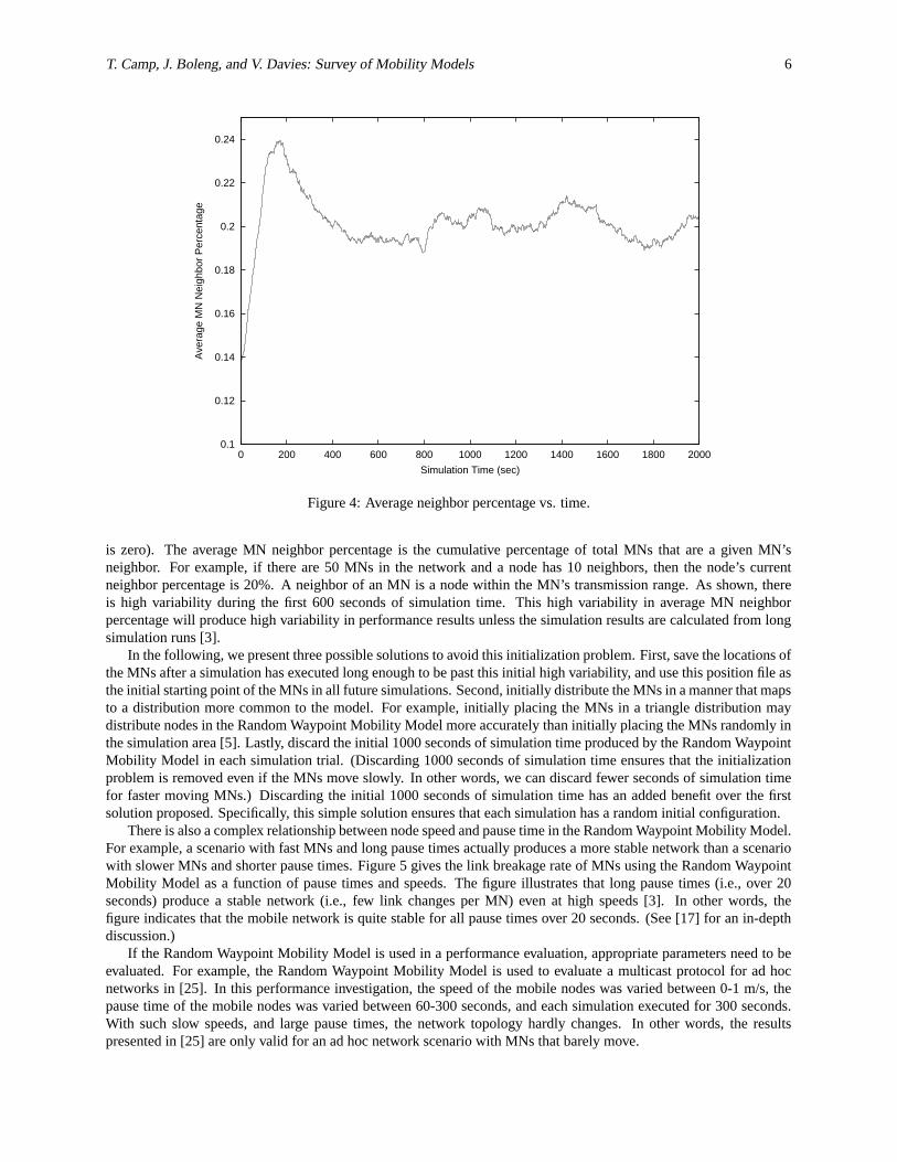
In most of the performance investigations that use the Random Waypoint Mobility Model, the MNs are initiallydistributed randomly around the simulation area. This initial random distribution of MNs is not representative of themanner in which nodes distribute themselves when moving. Figure 4 illustrates the cumulative average MN neighborpercentage for MNs using the Random Waypoint Mobility Model as time progresses (speed is 1 m/s and pause time


0.1

0.12

0.14

0.16

0.18

0.2

0.22

0.24

0 200 400 600 800 1000 1200 1400 1600 1800 2000

Ave

rage

MN

Nei

ghbo

r P

erce

ntag

e

Simulation Time (sec)

Figure 4: Average neighbor percentage vs. time.

is zero). The average MN neighbor percentage is the cumulative percentage of total MNs that are a given MN’sneighbor. For example, if there are 50 MNs in the network and a node has 10 neighbors, then the node’s currentneighbor percentage is 20%. A neighbor of an MN is a node within the MN’s transmission range. As shown, thereis high variability during the first 600 seconds of simulation time. This high variability in average MN neighborpercentage will produce high variability in performance results unless the simulation results are calculated from longsimulation runs [3].

In the following, we present three possible solutions to avoid this initialization problem. First, save the locations ofthe MNs after a simulation has executed long enough to be past this initial high variability, and use this position file asthe initial starting point of the MNs in all future simulations. Second, initially distribute the MNs in a manner that mapsto a distribution more common to the model. For example, initially placing the MNs in a triangle distribution maydistribute nodes in the Random Waypoint Mobility Model more accurately than initially placing the MNs randomly inthe simulation area [5]. Lastly, discard the initial 1000 seconds of simulation time produced by the Random WaypointMobility Model in each simulation trial. (Discarding 1000 seconds of simulation time ensures that the initializationproblem is removed even if the MNs move slowly. In other words, we can discard fewer seconds of simulation timefor faster moving MNs.) Discarding the initial 1000 seconds of simulation time has an added benefit over the firstsolution proposed. Specifically, this simple solution ensures that each simulation has a random initial configuration.

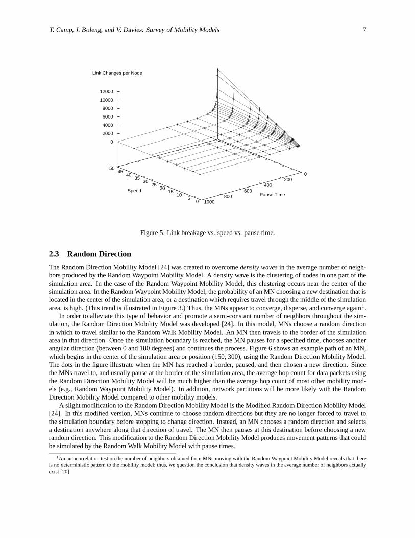
There is also a complex relationship between node speed and pause time in the Random Waypoint Mobility Model.For example, a scenario with fast MNs and long pause times actually produces a more stable network than a scenariowith slower MNs and shorter pause times. Figure 5 gives the link breakage rate of MNs using the Random WaypointMobility Model as a function of pause times and speeds. The figure illustrates that long pause times (i.e., over 20seconds) produce a stable network (i.e., few link changes per MN) even at high speeds [3]. In other words, thefigure indicates that the mobile network is quite stable for all pause times over 20 seconds. (See [17] for an in-depthdiscussion.)

If the Random Waypoint Mobility Model is used in a performance evaluation, appropriate parameters need to beevaluated. For example, the Random Waypoint Mobility Model is used to evaluate a multicast protocol for ad hocnetworks in [25]. In this performance investigation, the speed of the mobile nodes was varied between 0-1 m/s, thepause time of the mobile nodes was varied between 60-300 seconds, and each simulation executed for 300 seconds.With such slow speeds, and large pause times, the network topology hardly changes. In other words, the resultspresented in [25] are only valid for an ad hoc network scenario with MNs that barely move.


05

1015

2025

3035

4045

50

Speed

0200

400600

8001000

Pause Time

0

2000

4000

6000

8000

10000

12000

Link Changes per Node

Figure 5: Link breakage vs. speed vs. pause time.

2.3 Random Direction

The Random Direction Mobility Model [24] was created to overcome density waves in the average number of neigh-bors produced by the Random Waypoint Mobility Model. A density wave is the clustering of nodes in one part of thesimulation area. In the case of the Random Waypoint Mobility Model, this clustering occurs near the center of thesimulation area. In the Random Waypoint Mobility Model, the probability of an MN choosing a new destination that islocated in the center of the simulation area, or a destination which requires travel through the middle of the simulationarea, is high. (This trend is illustrated in Figure 3.) Thus, the MNs appear to converge, disperse, and converge again1.

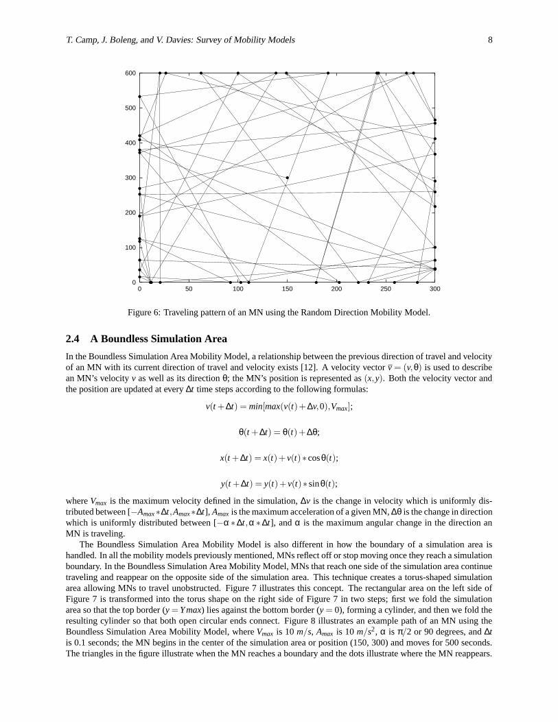
In order to alleviate this type of behavior and promote a semi-constant number of neighbors throughout the sim-ulation, the Random Direction Mobility Model was developed [24]. In this model, MNs choose a random directionin which to travel similar to the Random Walk Mobility Model. An MN then travels to the border of the simulationarea in that direction. Once the simulation boundary is reached, the MN pauses for a specified time, chooses anotherangular direction (between 0 and 180 degrees) and continues the process. Figure 6 shows an example path of an MN,which begins in the center of the simulation area or position (150, 300), using the Random Direction Mobility Model.The dots in the figure illustrate when the MN has reached a border, paused, and then chosen a new direction. Sincethe MNs travel to, and usually pause at the border of the simulation area, the average hop count for data packets usingthe Random Direction Mobility Model will be much higher than the average hop count of most other mobility mod-els (e.g., Random Waypoint Mobility Model). In addition, network partitions will be more likely with the RandomDirection Mobility Model compared to other mobility models.

A slight modification to the Random Direction Mobility Model is the Modified Random Direction Mobility Model[24]. In this modified version, MNs continue to choose random directions but they are no longer forced to travel tothe simulation boundary before stopping to change direction. Instead, an MN chooses a random direction and selectsa destination anywhere along that direction of travel. The MN then pauses at this destination before choosing a newrandom direction. This modification to the Random Direction Mobility Model produces movement patterns that couldbe simulated by the Random Walk Mobility Model with pause times.

1An autocorrelation test on the number of neighbors obtained from MNs moving with the Random Waypoint Mobility Model reveals that thereis no deterministic pattern to the mobility model; thus, we question the conclusion that density waves in the average number of neighbors actuallyexist [20]


0

100

200

300

400

500

600

0 50 100 150 200 250 300

Figure 6: Traveling pattern of an MN using the Random Direction Mobility Model.

2.4 A Boundless Simulation Area

In the Boundless Simulation Area Mobility Model, a relationship between the previous direction of travel and velocityof an MN with its current direction of travel and velocity exists [12]. A velocity vector v = (v,θ) is used to describean MN’s velocity v as well as its direction θ; the MN’s position is represented as (x,y). Both the velocity vector andthe position are updated at every ∆t time steps according to the following formulas:

v(t +∆t) = min[max(v(t)+∆v,0),Vmax];

θ(t +∆t) = θ(t)+∆θ;

x(t +∆t) = x(t)+ v(t)∗ cosθ(t);

y(t +∆t) = y(t)+ v(t)∗ sinθ(t);

where Vmax is the maximum velocity defined in the simulation, ∆v is the change in velocity which is uniformly dis-tributed between [−Amax∗∆t,Amax∗∆t], Amax is the maximum acceleration of a given MN, ∆θ is the change in directionwhich is uniformly distributed between [−α ∗∆t,α ∗∆t], and α is the maximum angular change in the direction anMN is traveling.

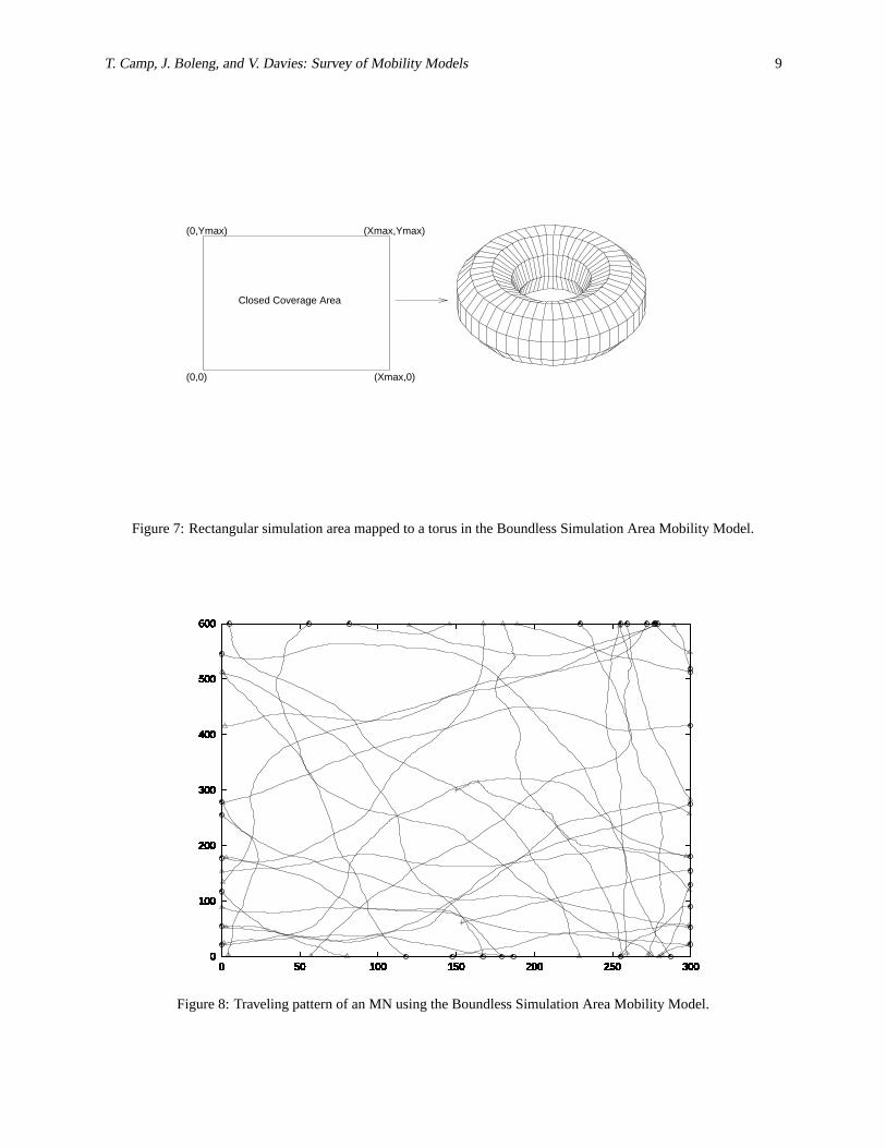
The Boundless Simulation Area Mobility Model is also different in how the boundary of a simulation area ishandled. In all the mobility models previously mentioned, MNs reflect off or stop moving once they reach a simulationboundary. In the Boundless Simulation Area Mobility Model, MNs that reach one side of the simulation area continuetraveling and reappear on the opposite side of the simulation area. This technique creates a torus-shaped simulationarea allowing MNs to travel unobstructed. Figure 7 illustrates this concept. The rectangular area on the left side ofFigure 7 is transformed into the torus shape on the right side of Figure 7 in two steps; first we fold the simulationarea so that the top border (y = Y max) lies against the bottom border (y = 0), forming a cylinder, and then we fold theresulting cylinder so that both open circular ends connect. Figure 8 illustrates an example path of an MN using theBoundless Simulation Area Mobility Model, where Vmax is 10 m/s, Amax is 10 m/s2, α is π/2 or 90 degrees, and ∆tis 0.1 seconds; the MN begins in the center of the simulation area or position (150, 300) and moves for 500 seconds.The triangles in the figure illustrate when the MN reaches a boundary and the dots illustrate where the MN reappears.


(Xmax,0)

(0,Ymax) (Xmax,Ymax)

(0,0)

Closed Coverage Area

Figure 7: Rectangular simulation area mapped to a torus in the Boundless Simulation Area Mobility Model.

0

100

200

300

400

500

600

0 50 100 150 200 250 3000

100

200

300

400

500

600

0 50 100 150 200 250 3000

100

200

300

400

500

600

0 50 100 150 200 250 3000

100

200

300

400

500

600

0 50 100 150 200 250 3000

100

200

300

400

500

600

0 50 100 150 200 250 3000

100

200

300

400

500

600

0 50 100 150 200 250 3000

100

200

300

400

500

600

0 50 100 150 200 250 3000

100

200

300

400

500

600

0 50 100 150 200 250 3000

100

200

300

400

500

600

0 50 100 150 200 250 3000

100

200

300

400

500

600

0 50 100 150 200 250 3000

100

200

300

400

500

600

0 50 100 150 200 250 3000

100

200

300

400

500

600

0 50 100 150 200 250 3000

100

200

300

400

500

600

0 50 100 150 200 250 3000

100

200

300

400

500

600

0 50 100 150 200 250 3000

100

200

300

400

500

600

0 50 100 150 200 250 3000

100

200

300

400

500

600

0 50 100 150 200 250 3000

100

200

300

400

500

600

0 50 100 150 200 250 3000

100

200

300

400

500

600

0 50 100 150 200 250 3000

100

200

300

400

500

600

0 50 100 150 200 250 3000

100

200

300

400

500

600

0 50 100 150 200 250 3000

100

200

300

400

500

600

0 50 100 150 200 250 3000

100

200

300

400

500

600

0 50 100 150 200 250 3000

100

200

300

400

500

600

0 50 100 150 200 250 3000

100

200

300

400

500

600

0 50 100 150 200 250 3000

100

200

300

400

500

600

0 50 100 150 200 250 3000

100

200

300

400

500

600

0 50 100 150 200 250 3000

100

200

300

400

500

600

0 50 100 150 200 250 3000

100

200

300

400

500

600

0 50 100 150 200 250 3000

100

200

300

400

500

600

0 50 100 150 200 250 3000

100

200

300

400

500

600

0 50 100 150 200 250 3000

100

200

300

400

500

600

0 50 100 150 200 250 3000

100

200

300

400

500

600

0 50 100 150 200 250 3000

100

200

300

400

500

600

0 50 100 150 200 250 3000

100

200

300

400

500

600

0 50 100 150 200 250 3000

100

200

300

400

500

600

0 50 100 150 200 250 3000

100

200

300

400

500

600

0 50 100 150 200 250 3000

100

200

300

400

500

600

0 50 100 150 200 250 3000

100

200

300

400

500

600

0 50 100 150 200 250 3000

100

200

300

400

500

600

0 50 100 150 200 250 3000

100

200

300

400

500

600

0 50 100 150 200 250 3000

100

200

300

400

500

600

0 50 100 150 200 250 3000

100

200

300

400

500

600

0 50 100 150 200 250 3000

100

200

300

400

500

600

0 50 100 150 200 250 3000

100

200

300

400

500

600

0 50 100 150 200 250 3000

100

200

300

400

500

600

0 50 100 150 200 250 3000

100

200

300

400

500

600

0 50 100 150 200 250 3000

100

200

300

400

500

600

0 50 100 150 200 250 3000

100

200

300

400

500

600

0 50 100 150 200 250 3000

100

200

300

400

500

600

0 50 100 150 200 250 3000

100

200

300

400

500

600

0 50 100 150 200 250 3000

100

200

300

400

500

600

0 50 100 150 200 250 3000

100

200

300

400

500

600

0 50 100 150 200 250 3000

100

200

300

400

500

600

0 50 100 150 200 250 3000

100

200

300

400

500

600

0 50 100 150 200 250 3000

100

200

300

400

500

600

0 50 100 150 200 250 3000

100

200

300

400

500

600

0 50 100 150 200 250 3000

100

200

300

400

500

600

0 50 100 150 200 250 3000

100

200

300

400

500

600

0 50 100 150 200 250 3000

100

200

300

400

500

600

0 50 100 150 200 250 3000

100

200

300

400

500

600

0 50 100 150 200 250 3000

100

200

300

400

500

600

0 50 100 150 200 250 3000

100

200

300

400

500

600

0 50 100 150 200 250 3000

100

200

300

400

500

600

0 50 100 150 200 250 3000

100

200

300

400

500

600

0 50 100 150 200 250 3000

100

200

300

400

500

600

0 50 100 150 200 250 3000

100

200

300

400

500

600

0 50 100 150 200 250 3000

100

200

300

400

500

600

0 50 100 150 200 250 3000

100

200

300

400

500

600

0 50 100 150 200 250 3000

100

200

300

400

500

600

0 50 100 150 200 250 3000

100

200

300

400

500

600

0 50 100 150 200 250 3000

100

200

300

400

500

600

0 50 100 150 200 250 3000

100

200

300

400

500

600

0 50 100 150 200 250 3000

100

200

300

400

500

600

0 50 100 150 200 250 3000

100

200

300

400

500

600

0 50 100 150 200 250 3000

100

200

300

400

500

600

0 50 100 150 200 250 3000

100

200

300

400

500

600

0 50 100 150 200 250 3000

100

200

300

400

500

600

0 50 100 150 200 250 3000

100

200

300

400

500

600

0 50 100 150 200 250 3000

100

200

300

400

500

600

0 50 100 150 200 250 3000

100

200

300

400

500

600

0 50 100 150 200 250 3000

100

200

300

400

500

600

0 50 100 150 200 250 3000

100

200

300

400

500

600

0 50 100 150 200 250 3000

100

200

300

400

500

600

0 50 100 150 200 250 3000

100

200

300

400

500

600

0 50 100 150 200 250 3000

100

200

300

400

500

600

0 50 100 150 200 250 3000

100

200

300

400

500

600

0 50 100 150 200 250 3000

100

200

300

400

500

600

0 50 100 150 200 250 3000

100

200

300

400

500

600

0 50 100 150 200 250 3000

100

200

300

400

500

600

0 50 100 150 200 250 3000

100

200

300

400

500

600

0 50 100 150 200 250 3000

100

200

300

400

500

600

0 50 100 150 200 250 3000

100

200

300

400

500

600

0 50 100 150 200 250 3000

100

200

300

400

500

600

0 50 100 150 200 250 3000

100

200

300

400

500

600

0 50 100 150 200 250 3000

100

200

300

400

500

600

0 50 100 150 200 250 3000

100

200

300

400

500

600

0 50 100 150 200 250 3000

100

200

300

400

500

600

0 50 100 150 200 250 3000

100

200

300

400

500

600

0 50 100 150 200 250 3000

100

200

300

400

500

600

0 50 100 150 200 250 3000

100

200

300

400

500

600

0 50 100 150 200 250 3000

100

200

300

400

500

600

0 50 100 150 200 250 3000

100

200

300

400

500

600

0 50 100 150 200 250 3000

100

200

300

400

500

600

0 50 100 150 200 250 3000

100

200

300

400

500

600

0 50 100 150 200 250 3000

100

200

300

400

500

600

0 50 100 150 200 250 300

Figure 8: Traveling pattern of an MN using the Boundless Simulation Area Mobility Model.


2.5 Gauss-Markov

The Gauss-Markov Mobility Model was originally proposed for the simulation of a PCS [19]; however, this modelhas been used for the simulation of an ad hoc network protocol [31]. In this section, we describe how the model wasimplemented in [31].

The Gauss-Markov Mobility Model was designed to adapt to different levels of randomness via one tuning pa-rameter. Initially each MN is assigned a current speed and direction. At fixed intervals of time, n, movement occursby updating the speed and direction of each MN. Specifically, the value of speed and direction at the nth instanceis calculated based upon the value of speed and direction at the (n−1)st instance and a random variable using thefollowing equations:

sn = αsn−1 +(1−α)s+√

(1−α2)sxn−1

dn = αdn−1 +(1−α)d +√

(1−α2)dxn−1

where sn and dn are the new speed and direction of the MN at time interval n; α, where 0 ≤ α ≤ 1, is the tuningparameter used to vary the randomness; s and d are constants representing the mean value of speed and direction asn → ∞; and sxn−1 and dxn−1 are random variables from a Gaussian distribution. Totally random values (or Brownianmotion) are obtained by setting α = 0 and linear motion is obtained by setting α = 1 [19]. Intermediate levels ofrandomness are obtained by varying the value of α between 0 and 1.

At each time interval the next location is calculated based on the current location, speed, and direction of move-ment. Specifically, at time interval n, an MN’s position is given by the equations:

xn = xn−1 + sn−1 cosdn−1

yn = yn−1 + sn−1 sindn−1

where (xn,yn) and (xn−1,yn−1) are the x and y coordinates of the MN’s position at the nth and (n−1)st time intervals,respectively, and sn−1 and dn−1 are the speed and direction of the MN, respectively, at the (n−1)st time interval.

To ensure that an MN does not remain near an edge of the grid for a long period of time, the MNs are forced awayfrom an edge when they move within a certain distance of the edge. This is done by modifying the mean directionvariable d in the above direction equation. For example, when an MN is near the right edge of the simulation grid, thevalue d is changed to 180 degrees. Thus, the MN’s new direction is away from the right edge of the simulation grid.The values of mean direction for different locations in the simulation grid are shown in Figure 9.

Figure 10 illustrates an example traveling pattern of an MN using the Gauss-Markov Mobility Model; the MNbegins its movement in the center of the simulation area or position (150, 300) and moves for 1000 seconds. InFigure 10, n is 1 second, α is 0.75, sxn−1 and dxn−1 are chosen from a random Gaussian distribution with mean equalto zero and standard deviation equal to one. The value of s is fixed at 10 m/s; the value of d is initially 90 degrees butchanges over time according to the edge proximity of the node.

As shown in Figure 10, the Gauss-Markov Mobility Model can eliminate the sudden stops and sharp turns encoun-tered in the Random Walk Mobility Model (see Section 2.1) by allowing past velocities (and directions) to influencefuture velocities (and directions).

The above description is how the Gauss-Markov Mobility Model was implemented in [31]. Other implementationsof the model exist. For example, the Markov process can be applied to the x and y equations directly instead of throughspeed and direction variables; in addition, a velocity vector can be used instead of a direction equation.

2.6 A Probabilistic Version of Random Walk

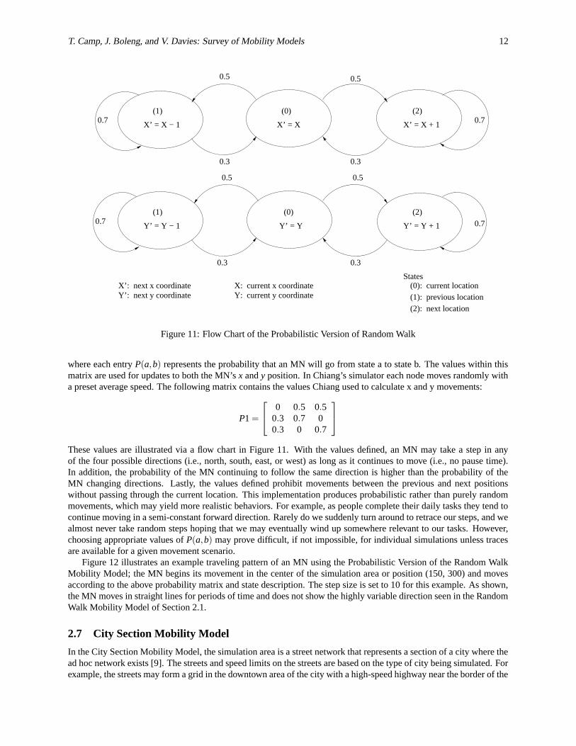
Chiang’s mobility model utilizes a probability matrix to determine the position of a particular MN in the next timestep, which is represented by three different states for position x and three different states for position y [7]. State 0represents the current (x or y) position of a given MN, state 1 represents the MN’s previous (x or y) position, and state2 represents the MN’s next position if the MN continues to move in the same direction. The probability matrix used is

P =

P(0,0) P(0,1) P(0,2)P(1,0) P(1,1) P(1,2)P(2,0) P(2,1) P(2,2)


mean=0

mean=90

mean=270

mean = 180

mean=45 mean=135

mean=225mean=315

Figure 9: Change of Mean Angle Near the Edges (in degrees)

0

100

200

300

400

500

600

0 50 100 150 200 250 3000

100

200

300

400

500

600

0 50 100 150 200 250 3000

100

200

300

400

500

600

0 50 100 150 200 250 300

Figure 10: Traveling pattern of an MN using the Gauss-Markov Mobility Model.


X’ = X − 1

(1)

(1)

Y’ = Y − 1

Y’: next y coordinate Y: current y coordinateX’: next x coordinate X: current x coordinate

(0)

X’ = X

(0)

Y’ = Y

(2)

Y’ = Y + 1

(2)

X’ = X + 1

0.5

0.7

0.70.7

0.7

0.5

0.50.5

0.3

0.30.3

0.3

States(0): current location(1): previous location(2): next location

Figure 11: Flow Chart of the Probabilistic Version of Random Walk

where each entry P(a,b) represents the probability that an MN will go from state a to state b. The values within thismatrix are used for updates to both the MN’s x and y position. In Chiang’s simulator each node moves randomly witha preset average speed. The following matrix contains the values Chiang used to calculate x and y movements:

P1 =

0 0.5 0.50.3 0.7 00.3 0 0.7

These values are illustrated via a flow chart in Figure 11. With the values defined, an MN may take a step in anyof the four possible directions (i.e., north, south, east, or west) as long as it continues to move (i.e., no pause time).In addition, the probability of the MN continuing to follow the same direction is higher than the probability of theMN changing directions. Lastly, the values defined prohibit movements between the previous and next positionswithout passing through the current location. This implementation produces probabilistic rather than purely randommovements, which may yield more realistic behaviors. For example, as people complete their daily tasks they tend tocontinue moving in a semi-constant forward direction. Rarely do we suddenly turn around to retrace our steps, and wealmost never take random steps hoping that we may eventually wind up somewhere relevant to our tasks. However,choosing appropriate values of P(a,b) may prove difficult, if not impossible, for individual simulations unless tracesare available for a given movement scenario.

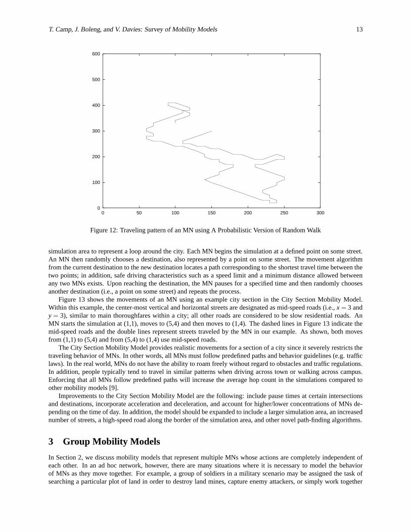
Figure 12 illustrates an example traveling pattern of an MN using the Probabilistic Version of the Random WalkMobility Model; the MN begins its movement in the center of the simulation area or position (150, 300) and movesaccording to the above probability matrix and state description. The step size is set to 10 for this example. As shown,the MN moves in straight lines for periods of time and does not show the highly variable direction seen in the RandomWalk Mobility Model of Section 2.1.

2.7 City Section Mobility Model

In the City Section Mobility Model, the simulation area is a street network that represents a section of a city where thead hoc network exists [9]. The streets and speed limits on the streets are based on the type of city being simulated. Forexample, the streets may form a grid in the downtown area of the city with a high-speed highway near the border of the


0

100

200

300

400

500

600

0 50 100 150 200 250 300

Figure 12: Traveling pattern of an MN using A Probabilistic Version of Random Walk

simulation area to represent a loop around the city. Each MN begins the simulation at a defined point on some street.An MN then randomly chooses a destination, also represented by a point on some street. The movement algorithmfrom the current destination to the new destination locates a path corresponding to the shortest travel time between thetwo points; in addition, safe driving characteristics such as a speed limit and a minimum distance allowed betweenany two MNs exists. Upon reaching the destination, the MN pauses for a specified time and then randomly choosesanother destination (i.e., a point on some street) and repeats the process.

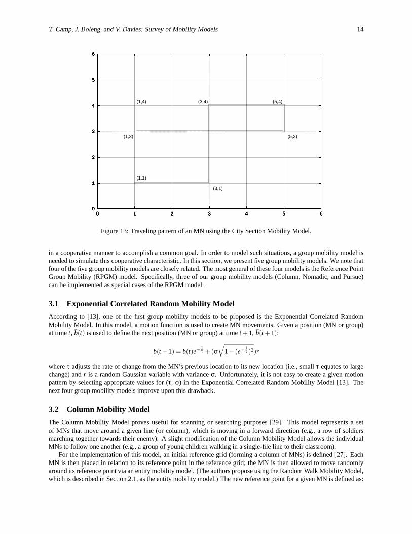
Figure 13 shows the movements of an MN using an example city section in the City Section Mobility Model.Within this example, the center-most vertical and horizontal streets are designated as mid-speed roads (i.e., x = 3 andy = 3), similar to main thoroughfares within a city; all other roads are considered to be slow residential roads. AnMN starts the simulation at (1,1), moves to (5,4) and then moves to (1,4). The dashed lines in Figure 13 indicate themid-speed roads and the double lines represent streets traveled by the MN in our example. As shown, both movesfrom (1,1) to (5,4) and from (5,4) to (1,4) use mid-speed roads.

The City Section Mobility Model provides realistic movements for a section of a city since it severely restricts thetraveling behavior of MNs. In other words, all MNs must follow predefined paths and behavior guidelines (e.g. trafficlaws). In the real world, MNs do not have the ability to roam freely without regard to obstacles and traffic regulations.In addition, people typically tend to travel in similar patterns when driving across town or walking across campus.Enforcing that all MNs follow predefined paths will increase the average hop count in the simulations compared toother mobility models [9].

Improvements to the City Section Mobility Model are the following: include pause times at certain intersectionsand destinations, incorporate acceleration and deceleration, and account for higher/lower concentrations of MNs de-pending on the time of day. In addition, the model should be expanded to include a larger simulation area, an increasednumber of streets, a high-speed road along the border of the simulation area, and other novel path-finding algorithms.

3 Group Mobility Models

In Section 2, we discuss mobility models that represent multiple MNs whose actions are completely independent ofeach other. In an ad hoc network, however, there are many situations where it is necessary to model the behaviorof MNs as they move together. For example, a group of soldiers in a military scenario may be assigned the task ofsearching a particular plot of land in order to destroy land mines, capture enemy attackers, or simply work together


0

1

2

3

4

5

6

0 1 2 3 4 5 60

1

2

3

4

5

6

0 1 2 3 4 5 60

1

2

3

4

5

6

0 1 2 3 4 5 60

1

2

3

4

5

6

0 1 2 3 4 5 60

1

2

3

4

5

6

0 1 2 3 4 5 60

1

2

3

4

5

6

0 1 2 3 4 5 6

(1,4)

(3,1)

(3,4) (5,4)

(5,3)(1,3)

(1,1)

Figure 13: Traveling pattern of an MN using the City Section Mobility Model.

in a cooperative manner to accomplish a common goal. In order to model such situations, a group mobility model isneeded to simulate this cooperative characteristic. In this section, we present five group mobility models. We note thatfour of the five group mobility models are closely related. The most general of these four models is the Reference PointGroup Mobility (RPGM) model. Specifically, three of our group mobility models (Column, Nomadic, and Pursue)can be implemented as special cases of the RPGM model.

3.1 Exponential Correlated Random Mobility Model

According to [13], one of the first group mobility models to be proposed is the Exponential Correlated RandomMobility Model. In this model, a motion function is used to create MN movements. Given a position (MN or group)at time t,~b(t) is used to define the next position (MN or group) at time t +1,~b(t +1):

b(t +1) = b(t)e−1τ +(σ

√

1− (e−1τ )2)r

where τ adjusts the rate of change from the MN’s previous location to its new location (i.e., small τ equates to largechange) and r is a random Gaussian variable with variance σ. Unfortunately, it is not easy to create a given motionpattern by selecting appropriate values for (τ, σ) in the Exponential Correlated Random Mobility Model [13]. Thenext four group mobility models improve upon this drawback.

3.2 Column Mobility Model

The Column Mobility Model proves useful for scanning or searching purposes [29]. This model represents a setof MNs that move around a given line (or column), which is moving in a forward direction (e.g., a row of soldiersmarching together towards their enemy). A slight modification of the Column Mobility Model allows the individualMNs to follow one another (e.g., a group of young children walking in a single-file line to their classroom).

For the implementation of this model, an initial reference grid (forming a column of MNs) is defined [27]. EachMN is then placed in relation to its reference point in the reference grid; the MN is then allowed to move randomlyaround its reference point via an entity mobility model. (The authors propose using the Random Walk Mobility Model,which is described in Section 2.1, as the entity mobility model.) The new reference point for a given MN is defined as:


anglereference grid

reference point

MN

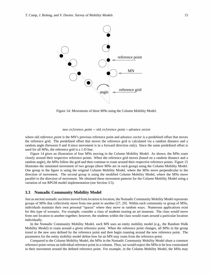
Figure 14: Movements of three MNs using the Column Mobility Model.

new re f erence point = old re f erence point +advance vector

where old reference point is the MN’s previous reference point and advance vector is a predefined offset that movesthe reference grid. The predefined offset that moves the reference grid is calculated via a random distance and arandom angle (between 0 and π since movement is in a forward direction only). Since the same predefined offset isused for all MNs, the reference grid is a 1-D line.

Figure 14 gives an illustration of four MNs moving in the Column Mobility Model. As shown, the MNs roamclosely around their respective reference points. When the reference grid moves (based on a random distance and arandom angle), the MNs follow the grid and then continue to roam around their respective reference points. Figure 15illustrates the simulated movement of two groups (three MNs are in each group) using the Column Mobility Model.One group in the figure is using the original Column Mobility Model, where the MNs move perpendicular to thedirection of movement. The second group is using the modified Column Mobility Model, where the MNs moveparallel to the direction of movement. We obtained these movement patterns for the Column Mobility Model using avariation of our RPGM model implementation (see Section 3.5).

3.3 Nomadic Community Mobility Model

Just as ancient nomadic societies moved from location to location, the Nomadic Community Mobility Model representsgroups of MNs that collectively move from one point to another [27, 29]. Within each community or group of MNs,individuals maintain their own personal ”spaces” where they move in random ways. Numerous applications existfor this type of scenario. For example, consider a class of students touring an art museum. The class would movefrom one location to another together; however, the students within the class would roam around a particular locationindividually.

In the Nomadic Community Mobility Model, each MN uses an entity mobility model (e.g., the Random WalkMobility Model) to roam around a given reference point. When the reference point changes, all MNs in the grouptravel to the new area defined by the reference point and then begin roaming around the new reference point. Theparameters for the entity mobility model define how far an MN may roam from the reference point.

Compared to the Column Mobility Model, the MNs in the Nomadic Community Mobility Model share a commonreference point versus an individual reference point in a column. Thus, we would expect the MNs to be less constrainedin their movement around the defined reference point. For example, in the Column Mobility Model, the MNs may


0

100

200

300

400

500

600

0 50 100 150 200 250 300

Original Mode (parallel to direction)

0

100

200

300

400

500

600

0 50 100 150 200 250 3000

100

200

300

400

500

600

0 50 100 150 200 250 3000

100

200

300

400

500

600

0 50 100 150 200 250 300

Modified Mode (perpendicular to direction)

0

100

200

300

400

500

600

0 50 100 150 200 250 3000

100

200

300

400

500

600

0 50 100 150 200 250 300

Figure 15: Traveling pattern of MNs using the Column Mobility Model.

Figure 16: Movements of seven MNs using the Nomadic Community Mobility Model.


Figure 17: Movements of six MNs using the Pursue Mobility Model.

only travel for two seconds before changing direction and speed; in the Nomadic Community Mobility Model, theMNs may be allowed to travel for 60 seconds before changing direction and speed. Figure 16 gives an illustration ofseven MNs moving with the Nomadic Community Mobility Model. The reference point (represented by a small blackdot) moves from one location to another; as shown, the MNs follow the movement of the reference point. While we donot illustrate a simulated movement pattern for the Nomadic Community Mobility Model, one could easily be createdby using the implementation of the RPGM model (see Section 3.5).

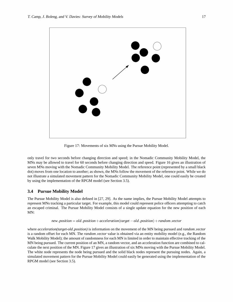
3.4 Pursue Mobility Model

The Pursue Mobility Model is also defined in [27, 29]. As the name implies, the Pursue Mobility Model attempts torepresent MNs tracking a particular target. For example, this model could represent police officers attempting to catchan escaped criminal. The Pursue Mobility Model consists of a single update equation for the new position of eachMN:

new position = old position+acceleration(target −old position)+ random vector

where acceleration(target-old position) is information on the movement of the MN being pursued and random vectoris a random offset for each MN. The random vector value is obtained via an entity mobility model (e.g., the RandomWalk Mobility Model); the amount of randomness for each MN is limited in order to maintain effective tracking of theMN being pursued. The current position of an MN, a random vector, and an acceleration function are combined to cal-culate the next position of the MN. Figure 17 gives an illustration of six MNs moving with the Pursue Mobility Model.The white node represents the node being pursued and the solid black nodes represent the pursuing nodes. Again, asimulated movement pattern for the Pursue Mobility Model could easily be generated using the implementation of theRPGM model (see Section 3.5).


GM

RP(t)

RP(t+1)

RM

MN

Figure 18: Movements of three MNs using the RPGM model.

3.5 Reference Point Group Mobility Model

The Reference Point Group Mobility (RPGM) model represents the random motion of a group of MNs as well as therandom motion of each individual MN within the group [13]. Group movements are based upon the path traveled bya logical center for the group. The logical center for the group is used to calculate group motion via a group motionvector, ~GM. The motion of the group center completely characterizes the movement of its corresponding group ofMNs, including their direction and speed. Individual MNs randomly move about their own pre-defined referencepoints, whose movements depend on the group movement. As the individual reference points move from time t tot +1, their locations are updated according to the group’s logical center. Once the updated reference points, RP(t +1),are calculated, they are combined with a random motion vector, ~RM, to represent the random motion of each MNabout its individual reference point.

Figure 18 gives an illustration of three MNs moving with the RPGM model. The figure illustrates that, at time t,three black dots exist to represent the reference points, RP(t), for the three MNs. As shown, the RPGM model usesa group motion vector ~GM to calculate each MN’s new reference point, RP(t + 1), at time t + 1; as stated, ~GM maybe randomly chosen or predefined. The new position for each MN is then calculated by summing a random motionvector, ~RM, with the new reference point. The length of ~RM is uniformly distributed within a specified radius centeredat RP(t +1) and its direction is uniformly distributed between 0 and 2π.

Movement patterns using the RPGM model are shown in Figures 19 and 20. Figure 19 is an illustration of threeMNs moving together as one group. Figure 20 is an illustration of five groups moving, such that each group hasa different number of MNs. Both the movement of the logical center for each group, and the random motion ofeach individual MN within the group, are implemented via the Random Waypoint Mobility Model. One difference,however, is that individual MNs do not use pause times while the group is moving. Pause times are only used whenthe group reference point reaches a destination and all group nodes pause for the same period of time.

The RPGM model was designed to depict scenarios such as an avalanche rescue. During an avalanche rescue, theresponding team consisting of human and canine members work cooperatively. The human guides tend to set a generalpath for the dogs to follow, since they usually know the approximate location of victims. The dogs each create their


0

100

200

300

400

500

600

0 50 100 150 200 250 3000

100

200

300

400

500

600

0 50 100 150 200 250 3000

100

200

300

400

500

600

0 50 100 150 200 250 300

Figure 19: Traveling pattern of one group (three MNs) using the RPGM model.

0

100

200

300

400

500

600

0 50 100 150 200 250 300

2 nodes

0

100

200

300

400

500

600

0 50 100 150 200 250 3000

100

200

300

400

500

600

0 50 100 150 200 250 300

3 nodes

0

100

200

300

400

500

600

0 50 100 150 200 250 3000

100

200

300

400

500

600

0 50 100 150 200 250 3000

100

200

300

400

500

600

0 50 100 150 200 250 300

4 nodes

0

100

200

300

400

500

600

0 50 100 150 200 250 3000

100

200

300

400

500

600

0 50 100 150 200 250 3000

100

200

300

400

500

600

0 50 100 150 200 250 3000

100

200

300

400

500

600

0 50 100 150 200 250 300

5 nodes

0

100

200

300

400

500

600

0 50 100 150 200 250 3000

100

200

300

400

500

600

0 50 100 150 200 250 3000

100

200

300

400

500

600

0 50 100 150 200 250 3000

100

200

300

400

500

600

0 50 100 150 200 250 3000

100

200

300

400

500

600

0 50 100 150 200 250 300

6 nodes

0

100

200

300

400

500

600

0 50 100 150 200 250 3000

100

200

300

400

500

600

0 50 100 150 200 250 3000

100

200

300

400

500

600

0 50 100 150 200 250 3000

100

200

300

400

500

600

0 50 100 150 200 250 3000

100

200

300

400

500

600

0 50 100 150 200 250 300

Figure 20: Traveling pattern of five groups using the RPGM model.


Number of Number of Total Percent ofgroup members these groups nodes total

2 7 14 28%3 4 12 24%4 2 8 16%5 2 10 20%6 1 6 12%

TOTAL 16 50 100%

Table 1: Groups specified in the RPGM model.

own “random” paths around the general area chosen by their human counterparts.The RPGM model was originally defined in [13] and then used in [21]. If appropriate group paths are chosen,

along with proper initial locations for various groups, many different mobility applications may be represented withthe RPGM model. In [13], three applications for the RPGM model are defined. First, the In-place Mobility Modelpartitions a given geographical area such that each subset of the original area is assigned to a specific group; thespecified group then operates only within that geographic subset. Second, the Overlap Mobility Model simulatesseveral different groups, each of which has a different purpose, working in the same geographic region; each groupwithin this model may have different characteristics than other groups within the same geographical boundary. Forexample, in disaster recovery of a geographical area, one might encounter a rescue personnel team, a medical team,and a psychologist team, each of which have unique traveling patterns, speeds, and behaviors. Lastly, the ConventionMobility Model divides a given area into smaller subsets and allows the groups to move in a similar pattern throughouteach subset. Similar to the Overlap Mobility Model, some groups in the Convention Mobility Model may travel fasterthan others

As mentioned, Figure 15, which is an illustration of the Column Mobility Model, was created via our RPGMmodel implementation. To create this movement pattern, we added the following restriction to the RPGM model: allthe nodes’ reference points in a group must be in a column which is either perpendicular or parallel to the directionof travel. While simulated movement patterns are not illustrated in Sections 3.3 and 3.4, an implementation of theNomadic Community Mobility Model and the Pursue Mobility Model are obtained from our RPGM model imple-mentation. Specifically, we use a value of zero for the input parameter reference point separation in our RPGM modelimplementation to ensure that all the individual node reference points are the same as the group reference point.

4 Importance of Choosing a Mobility Model

In this section, we illustrate that the choice of a mobility model can have a significant effect on the performanceinvestigation of an ad hoc network protocol. The results presented illustrate the importance of choosing an appropriatemobility model (or models) for the performance evaluation of a given ad hoc network protocol.

We use ns-2 [23] to compare the performance of the Random Walk Mobility Model, the Random Waypoint Mo-bility Model, the Random Direction Mobility Model, and the Reference Point Group Mobility (RPGM) model via asimulation with 50 MNs. (Table 1 details how the 50 MNs are separated into groups for the RPGM model.) Two setsof results are presented for the RPGM model; one set of results consists of intergroup communication only, and theother set of results consists of 50% intergroup communication and 50% intragroup communication (see details be-low). Each MN in the simulations has a 100m transmission range, and the routing of packets is accomplished with theDynamic Source Routing Protocol (DSR) [16]. The parameters for these four mobility models were chosen in a wayto simulate path movements that were as similar as possible. For example, in the Random Walk Mobility Model, theMN changes directions after moving a distance of 100m, which produces movement patterns similar to the RandomWaypoint Mobility Model when pause time is zero.

DSR is a source routing protocol which determines routes on demand. In a source routing protocol, each packetcarries the full route (a sequenced list of nodes) that the packet should be able to traverse in its header. In an on demand(or reactive) routing protocol such as DSR, a route to a destination is requested only when there is data to send to thatdestination, and a route to that destination is unknown or expired. We chose DSR since it performs well in many of


50

60

70

80

90

100

0 5 10 15 20

Dat

a P

acke

t Del

iver

y R

atio

(%

)

Average Speed (m/s)

Random WaypointRPGM intragroup and intergroup

Random WalkRPGM all intergroup

Random Direction

Figure 21: Data packet delivery ratio vs. speed.

the performance evaluations of unicast routing protocols (e.g. [4, 15]).The ns-2 code used in our simulations of DSR was obtained from [22]. The simulations are executed for 2010

seconds; however, our results are gathered from 1010 seconds of simulated time and data is only sent from 1000-2000seconds of simulation time, which accounts for the conclusions drawn from Figure 4. Our communication model issimilar to the communication model used in [4] and [15]. For the entity mobility models and RPGM with all intergroupcommunication, we have 20 CBR (constant bit rate) sources sending packets at a rate of 1 packet per second to 20different receivers. In other words, 20,000 packets are transmitted between 20 peers. For the RPGM results withboth intergroup and intragroup communication, 10,000 packets are transmitted between 20 peers in different groups(1 packet every 2 seconds) and 10,000 packets are transmitted within groups (1 packet every 5 seconds). All packetsare of size 64 bytes. We avoid unnecessary contention in the transmission of packets by offsetting the transmission ofa data packet by 0.0001 seconds.

All the performance results presented are an average of 10 different simulation trials. The initial locations of theMNs in each trial are random (i.e., via the uniform distribution). We calculate a 95% confidence interval for theunknown mean, and we plot these confidence intervals on the figures. Since most of the confidence intervals are quitesmall (in fact, some of the intervals are smaller than the symbol used to represent the mean on our plots), we areconvinced that our simulation results precisely represent the unknown mean.

In our comparison of the four mobility models, we consider the following performance metrics obtained from theDSR protocol: data packet delivery ratio, end-to-end delay, average hop count, and protocol overhead. The data packetdelivery ratio is the ratio of the number of data packets delivered to the destination nodes divided by the number ofdata packets transmitted by the source nodes.

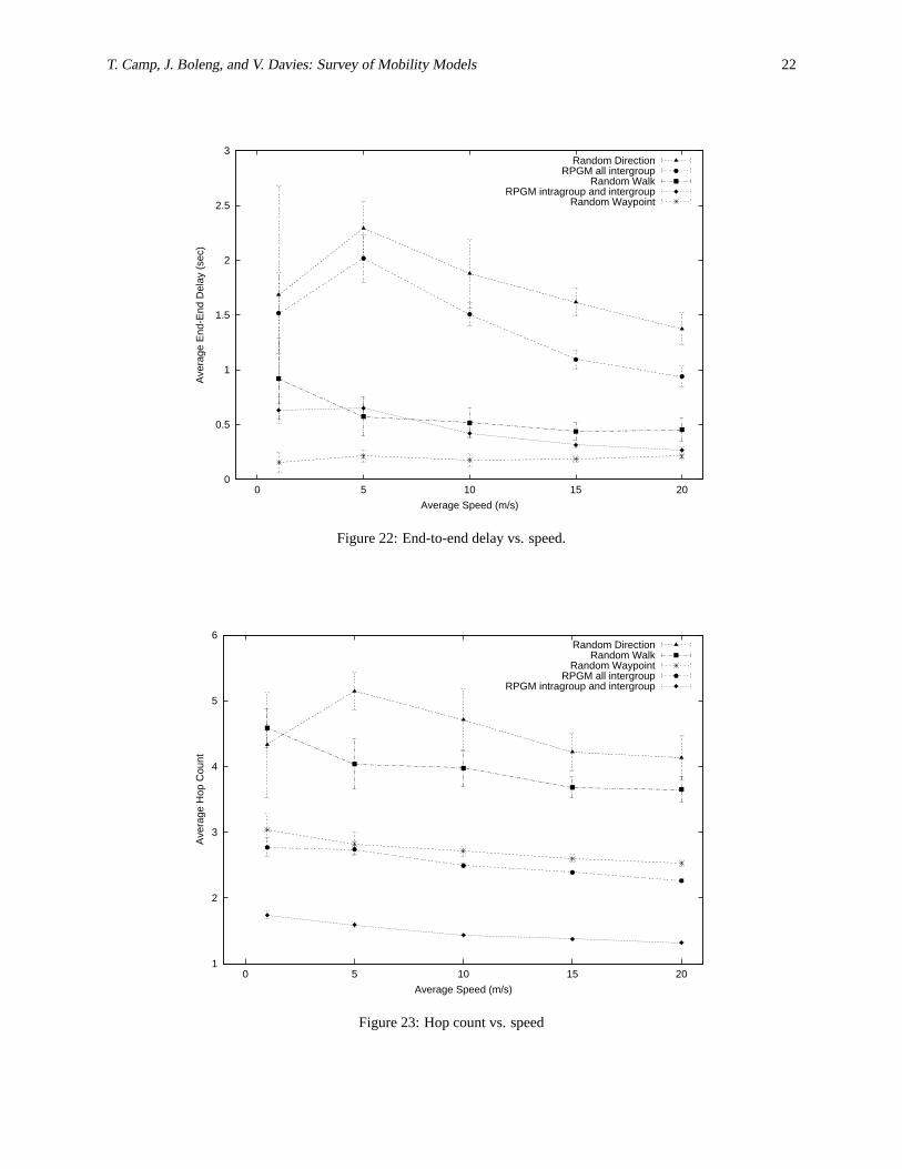
Figures 21 and 22 illustrate the performance (i.e., data packet delivery ratio and end-to-end delay) of DSR withthe four mobility models chosen. Figure 23 illustrates the average hop count versus speed, which helps us understandthese two performance figures. The three figures combine to illustrate that the Random Waypoint Mobility Modelstresses DSR less than the other two entity mobility models. Specifically, the Random Waypoint Mobility Model hasthe highest data packet delivery ratio, the lowest end-to-end delay, and the lowest average hop count compared tothe Random Walk Mobility Model and Random Direction Mobility Model. These results exist since MNs using theRandom Waypoint Mobility Model are often traveling through (or to) the center of the simulation area.

The Random Direction Mobility Model has the highest average hop count, the highest end-to-end delay, and thelowest data packet delivery ratio since the Random Direction Mobility Model has each MN move to the border of the


0

0.5

1

1.5

2

2.5

3

0 5 10 15 20

Ave

rage

End

-End

Del

ay (

sec)

Average Speed (m/s)

Random DirectionRPGM all intergroup

Random WalkRPGM intragroup and intergroup

Random Waypoint

Figure 22: End-to-end delay vs. speed.

1

2

3

4

5

6

0 5 10 15 20

Ave

rage

Hop

Cou

nt

Average Speed (m/s)

Random DirectionRandom Walk

Random WaypointRPGM all intergroup

RPGM intragroup and intergroup

Figure 23: Hop count vs. speed


0

5

10

15

20

25

30

35

0 5 10 15 20

Con

trol

Pac

ket T

rans

mis

sion

s pe

r D

ata

Pac

ket D

eliv

ered

Average Speed (m/s)

Random WalkRandom Direction

RPGM all intergroupRandom Waypoint


Figure 24: Control packet overhead vs. speed.

simulation area before changing direction. Thus, hop counts between a sender and receiver are higher and transientnetwork partitions are more likely in the Random Direction Mobility Model compared to the other two entity mobilitymodels. The performance of DSR when using the Random Walk Mobility Model falls between these two extremes.Lastly, we note that the confidence intervals of the Random Walk Mobility Model and Random Direction MobilityModel are the largest; more variation in movement patterns exist in these two mobility models.

The Reference Point Group Mobility (RPGM) model with only intergroup communication has approximately thesame hop count as the Random Waypoint Mobility Model (see Figure 23). As mentioned, both a group’s movementand an MN’s movement within a group in the RPGM model is done via the Random Waypoint Mobility Model. Thus,we would expect the hop counts for received packets to be similar between these two simulations. The RPGM modelwith only intergroup communication has a much lower data packet delivery ratio and higher end-to-end delay thanthe results for the Random Waypoint Mobility Model. Since only 16 groups exist (see Table 1) in the RPGM modelsimulation, the network will be much sparser than the 50 MNs that roam in the Random Waypoint Mobility Model.And, since all communication is between groups, the performance of the mobility model in terms of data packetdelivery ratio and end-to-end delay will suffer from transient partitions that exist in the sparse network.

The RPGM model with both intergroup and intragroup communication has the lowest average hop count (seeFigure 23), since 50% of the packets transmitted are sent within the groups. Low average hop count corresponds to ahigh data packet delivery ratio, which is illustrated in Figure 21. The data packet delivery ratio is not, however, as highas one would expect; since 50% of the packets are transmitted between groups, these packets are sometimes droppeddue to the transient partitions that occur. Figure 22 illustrates that the partitions also affect the end-to-end delay of theresults for the RPGM model with both intergroup and intragroup communication.

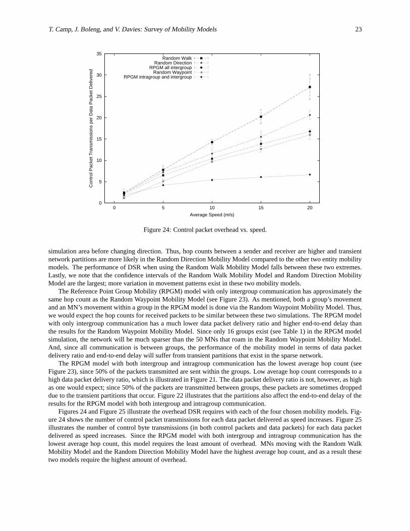
Figures 24 and Figure 25 illustrate the overhead DSR requires with each of the four chosen mobility models. Fig-ure 24 shows the number of control packet transmissions for each data packet delivered as speed increases. Figure 25illustrates the number of control byte transmissions (in both control packets and data packets) for each data packetdelivered as speed increases. Since the RPGM model with both intergroup and intragroup communication has thelowest average hop count, this model requires the least amount of overhead. MNs moving with the Random WalkMobility Model and the Random Direction Mobility Model have the highest average hop count, and as a result thesetwo models require the highest amount of overhead.


0

100

200

300

400

500

600

0 5 10 15 20

Con

trol

Byt

e T

rans

mis

sion

s pe

r D

ata

Pac

ket D

eliv

ered

Average Speed (m/s)

Random DirectionRandom Walk

RPGM all intergroupRandom Waypoint


Figure 25: Control byte overhead vs. speed

5 Conclusions

Conclusion 1: The performance of an ad hoc network protocol can vary significantly with different mobility models.Figures 21–25 illustrate the performance of one ad hoc network routing protocol with different mobility models. Asshown, the performance of the protocol is greatly affected by the mobility model.Conclusion 2: The performance of an ad hoc network protocol can vary significantly when the same mobility modelis used with different parameters. Figures 1 and 2 illustrate the widely different movement patterns that can occurwith the Random Walk Mobility Model when different input parameters are used. When evaluated, these differentmovement patterns lead to widely different performance results.Conclusion 3: The selection of a mobility model may require a data traffic pattern which significantly influences pro-tocol performance. For instance, if a group mobility model is simulated, then protocol evaluation should be done witha portion of the traffic local to the group. Intragroup communication changes a protocol’s performance dramatically,compared to the same mobility scenarios and all intergroup communication (see Figures 21–25).Conclusion 4: The performance of an ad hoc network protocol should be evaluated with the mobility model that mostclosely matches the expected real-world scenario. In fact, the anticipated real-world scenario can aid the developmentof the ad hoc network protocol significantly. However, since the development of ad hoc networks is relatively new,we do not yet know what a realistic model is for a given scenario. In fact, we are just beginning to see realistic tracefiles for PCS or cellular networks. In [30], results are presented on how often MNs move and how far they move forthe Metricom radio network. Traffic patterns and on-line behavior for wireless users of a high speed wireless accessnetwork are presented in [14].Conclusion 5: If the expected real-world scenario is unknown, then researchers should make an informed choice aboutthe mobility model to use2. The following list summarizes our conclusions for the seven synthetic entity mobilitymodels for ad hoc networks.

1. The Random Walk Mobility Model with a small input parameter (distance or time) produces Brownian motionand, therefore, basically evaluates a static network (see Figure 2) when used in a performance investigation. Alarge input parameter (distance or time) is similar to the Random Waypoint Mobility Model without pause times

2Since a single mobility model is unlikely to depict the behavior of the MNs in all scenarios, it may be best to evaluate an ad hoc networkprotocol with multiple mobility models.


(see Figure 1 and Figure 3). The main difference between these two mobility models is that MNs are more likelyto cluster in the center of the simulation area with the Random Waypoint Mobility Model.

2. The Random Waypoint Mobility Model is used in many prominent simulation studies of ad hoc network pro-tocols. It is flexible, and it appears to create realistic mobility patterns for the way people might move in, forexample, a conference setting or museum (see Figure 3). One concern with this model is the straight movementpattern created by the MN to the next chosen destination.

3. The Random Direction Mobility Model (see Figure 6) is an unrealistic model because it is unlikely that peoplewould spread themselves evenly throughout an area (a building or a city). In addition, it is unlikely that peoplewill only pause at the edge of a given area. The Modified Random Direction Mobility Model allows MNs topause and change directions before reaching the simulation boundary; this version, however, is identical to theRandom Walk Mobility Model with pause times.

4. The Boundless Simulation Area Mobility Model provides movement patterns that one might expect in the real-world (see Figure 8). In addition, this model is the only one that allows MNs to travel unobstructed in thesimulation area, thus removing any simulation edge effects from the performance evaluation. One concern,however, is the undesired side effects that would occur from allowing the MNs to move around a torus. Forexample, one static MN and one MN that continues to move in the same direction become neighbors again andagain. In addition, a simulation area without edges would force modification of the radio propagation model towrap transmissions from one edge of the area to the other.

5. The Gauss-Markov Mobility Model also provides movement patterns that one might expect in the real-world(see Figure 10), if appropriate parameters are chosen. In addition, the method used to force MNs away from theedges of the simulation area (thus avoiding undesired edge effects) is of note.

6. While the Probabilistic Random Walk Mobility Model also provides movement patterns that one might expectin the real-world (see Figure 12), choosing appropriate parameters for the probability matrix may be difficult.This model could become useful, however, when we have scenario trace data that we want to model.

7. The City Section Mobility Model (see Figure 13) appears to create realistic movements for a section of a city,since it severely restricts the traveling behavior of MNs; MNs do not have the ability to roam freely withoutregard to obstacles and other traffic regulations. Further development of this model (e.g., to use realistic citymaps) is desired.

Regarding the five synthetic group mobility models for ad hoc networks, the following list summarizes our conclusions.

1. The Exponential Correlated Random Mobility Model appears to theoretically describe all other mobility models.However, selecting appropriate parameter values is (almost) impossible.

2. The Column, Nomadic Community, and Pursue Mobility Models are useful group mobility models for specificrealistic scenarios. The movement patterns provided by these three mobility models can be obtained by changingthe parameters associated with the Reference Point Group Mobility Model.

3. The Reference Point Group Mobility Model (RPGM) is a generic method for handling group mobility. Anentity mobility model (or models) needs to be specified to handle both the movement of a group of MNs andthe movement of the individual MNs within the group. The input parameters of the RPGM model allow theflexibility to implement the Column, Nomadic Community, and Pursue Mobility Models.

In summary, if a group mobility model is desired, we recommend using the Reference Point Group Mobility Modelwith appropriate parameters. If an entity mobility model is desired, we recommend using either the Random WaypointMobility Model, the Random Walk Mobility Model (if clustering in the middle of the simulation area is undesired), orthe Gauss-Markov Mobility Model. However, a preferred entity mobility model combines the strengths of the currententity mobility models (see Conclusion 7). As mentioned, implementations of all the mobility models described inthis paper (except Exponential Correlated Random Mobility Model) are available at http://toilers.mines.edu. Ourimplementations allow a user to create either a gnuplot figure or an ns-2 mobility file of a given mobility model.Conclusion 6: The results of DSR presented in Figures 21–25 differ greatly from the results presented in [4] and[15]. As an example, all the data packet delivery ratios presented in [4] for DSR (using the Random Waypoint


Mobility Model) are over 95%. Their results are not comparable to ours because of the differences in our simulationenvironments. (For example, the maximum average speed considered in [4] is only 10 m/s; our maximum averagespeed is 20 m/s.) Furthermore, the metric used for the x-axes in [4] is pause time, rather than speed. As discussedin Section 2.2.2 (see Figure 5), speed has a much greater impact than pause time on link breakage rates [3]. Theresults presented in [15] are taken from only 250 seconds of simulation time. As shown in Figure 4, there is highvariability in the average number of neighbors during the initial seconds of simulation time for MNs using the randomwaypoint model. Since the authors of [15] do not present confidence intervals for the unknown mean in the randomscenarios, the precision of their estimates can not be determined. See [6] for more details on the differences betweenthe simulation environments in [4], [15], and herein.Conclusion 7: Further research on mobility models for ad hoc network protocol evaluation is needed. One avenue offuture work is to devote further effort in examining the movements of entities in the real world to produce accuratemobility models. A second avenue is to develop a new model that combines the best attributes of some of the models.For example, a new model could handle edges via the method in the Gauss-Markov Mobility Model and then combinethe movement patterns of the Boundless Simulation Area Mobility Model and the Random Waypoint (or RandomWalk) Mobility Model. A third avenue is to develop a minimum mobility model standard for performance evaluation.This minimum standard would allow us to evaluate different mobility models more thoroughly. Lastly, we shouldexamine the method used to choose a future MN location. In other words, the similarities and differences betweenmobility models that randomly select directions and mobility models that randomly select specific locations should beanalyzed.

References

[1] A. Bar-Noy, I. Kessler, and M. Sidi. Mobile users: To update or not to update? In Proceedings of the JointConference of the IEEE Computer and Communications Societies (INFOCOM), pages 570–576, 1994.

[2] S. Basagni, I. Chlamtac, V.R. Syrotiuk, and B.A. Woodward. A distance routing effect algorithm for mobility(DREAM). In Proceedings of the ACM/IEEE International Conference on Mobile Computing and Networking(MOBICOM), pages 76–84, 1998.

[3] J. Boleng. Normalizing mobility characteristics and enabling adaptive protocols for ad hoc networks. In Pro-ceedings of the Local and Metropolitan Area Networks Workshop (LANMAN), pages 9–12, March 2001.

[4] J. Broch, D. Maltz, D. Johnson, Y. Hu, and J. Jetcheva. Multi-hop wireless ad hoc network routing protocols. InProceedings of the ACM/IEEE International Conference on Mobile Computing and Networking (MOBICOM),pages 85–97, 1998.

[5] T.X. Brown. Personal correspondance. April 2001.

[6] T. Camp, J. Boleng, B. Williams, L. Wilcox, and W. Navidi. Performance evaluation of two location basedrouting protocols. In Proceedings of the Joint Conference of the IEEE Computer and Communications Societies(INFOCOM), 2002.

[7] C. Chiang. Wireless Network Multicasting. PhD thesis, University of California, Los Angeles, 1998.

[8] C. Chiang and M. Gerla. On-demand multicast in mobile wireless networks. In Proceedings of the IEEEInternational Conference on Network Protocols (ICNP), 1998.

[9] V. Davies. Evaluating mobility models within an ad hoc network. Master’s thesis, Colorado School of Mines,2000.

[10] J.J. Garcia-Luna-Aceves and E.L. Madrga. A multicast routing protocol for ad-hoc networks. In Proceedings ofthe Joint Conference of the IEEE Computer and Communications Societies (INFOCOM), pages 784–792, 1999.

[11] J.J. Garcia-Luna-Aceves and M. Spohn. Source-tree routing in wireless networks. In Proceedings of the 7thInternational Conference on Network Protocols (ICNP), 1999.

[12] Z. Haas. A new routing protocol for reconfigurable wireless networks. In Proceedings of the IEEE InternationalConference on Universal Personal Communications (ICUPC), pages 562–565, Oct. 1997.


[13] X. Hong, M. Gerla, G. Pei, and C. Chiang. A group mobility model for ad hoc wireless networks. In Proceedingsof the ACM International Workshop on Modeling and Simulation of Wireless and Mobile Systems (MSWiM),August 1999.

[14] R. Hutchins and E. W. Zegura. Measurements from a campus wireless network. In Proceedings of the IEEEInternational Conference on Communications (ICC), 2002.

[15] P. Johansson, T. Larsson, N. Hedman, B. Mielczarek, and M. Degermark. Routing protocols for mobile ad-hocnetworks - a comparative performance analysis. In Proceedings of the ACM/IEEE International Conference onMobile Computing and Networking (MOBICOM), pages 195–206, 1999.

[16] D. Johnson and D. Maltz. Dynamic source routing in ad hoc wireless networks. In T. Imelinsky and H. Korth,editors, Mobile Computing, pages 153–181. Kluwer Academic Publishers, 1996.

[17] B. Karp. Geographic Routing for Wireless Networks. PhD thesis, Harvard University, 2000.

[18] Y. Ko and N.H. Vaidya. Location-aided routing (LAR) in mobile ad hoc networks. In Proceedings of theACM/IEEE International Conference on Mobile Computing and Networking (MOBICOM), pages 66–75, 1998.

[19] B. Liang and Z. Haas. Predictive distance-based mobility management for PCS networks. In Proceedings of theJoint Conference of the IEEE Computer and Communications Societies (INFOCOM), March 1999.

[20] W. Navidi. Personal correspondance. October 2000.

[21] G. Pei, M. Gerla, X. Hong, and C. Chiang. A wireless hierarchical routing protocol with group mobility. InProceedings of the IEEE Wireless Communications and Networking Conference (WCNC), September 1999.

[22] The Rice University Monarch Project.Monarch extensions to the ns simulator. URL: http://www.monarch.cs.rice.edu/. Page accessed on May 30th,2002.

[23] The VINT Project. The network simulator - ns-2. http://www.isi.edu/nsnam/ns/. Page accessed on May 30th,2002.

[24] E. Royer, P.M. Melliar-Smith, and L. Moser. An analysis of the optimum node density for ad hoc mobilenetworks. In Proceedings of the IEEE International Conference on Communications (ICC), 2001.

[25] E.M. Royer and C. Perkins. Multicast operation of the ad-hoc on-demand distance vector routing protocol. InProceedings of the ACM/IEEE International Conference on Mobile Computing and Networking (MOBICOM),pages 207–218, 1999.

[26] I. Rubin and C. Choi. Impact of the location area structure on the performance of signaling channels in wirelesscellular networks. IEEE Communications Magazine, pages 108–115, 1997.

[27] M. Sanchez. Mobility models. http://www.disca.upv.es/misan/mobmodel.htm. Page accessed on May 30th, 2002.

[28] M. Sanchez and P. Manzoni. A java-based ad hoc networks simulator. In Proceedings of the SCS WesternMulticonference Web-based Simulation Track, Jan. 1999.

[29] M. Sanchez and P. Manzoni. Anejos: A java based simulator for ad-hoc networks. Future Generation ComputerSystems, 17(5):573–583, 2001.

[30] D. Tang and M. Baker. Analysis of a metropolitan-area wireless network. In Proceedings of the ACM/IEEEInternational Conference on Mobile Computing and Networking (MOBICOM), pages 13–23, 1999.

[31] V. Tolety. Load reduction in ad hoc networks using mobile servers. Master’s thesis, Colorado School of Mines,1999.

[32] E. W. Weisstein. The CRC Concise Encyclopedia of Mathematics. CRC Press, 1998.

[33] M. Zonoozi and P. Dassanayake. User mobility modeling and characterization of mobility pattern. IEEE Journalon Selected Areas in Communications, 15(7):1239–1252, 1997.

a survey of mobility models for ad hoc network research survey of mobility models for ad hoc...a...

Documents