a survey of butterfly diagrams for knots and links
TRANSCRIPT

University of Northern Iowa University of Northern Iowa
UNI ScholarWorks UNI ScholarWorks
Dissertations and Theses @ UNI Student Work
2017
A survey of butterfly diagrams for knots and links A survey of butterfly diagrams for knots and links
Mark Ronnenberg University of Northern Iowa
Let us know how access to this document benefits you
Copyright ©2017 Mark Ronnenberg
Follow this and additional works at: https://scholarworks.uni.edu/etd
Part of the Geometry and Topology Commons
Recommended Citation Recommended Citation Ronnenberg, Mark, "A survey of butterfly diagrams for knots and links" (2017). Dissertations and Theses @ UNI. 364. https://scholarworks.uni.edu/etd/364
This Open Access Thesis is brought to you for free and open access by the Student Work at UNI ScholarWorks. It has been accepted for inclusion in Dissertations and Theses @ UNI by an authorized administrator of UNI ScholarWorks. For more information, please contact [email protected].
A SURVEY OF BUTTERFLY DIAGRAMS FOR KNOTS AND LINKS
An Abstract of a ThesisSubmitted
in Partial Fulfillmentof the Requirement for the Degree
Master of Arts
Mark RonnenbergUniversity of Northern Iowa
May 2017
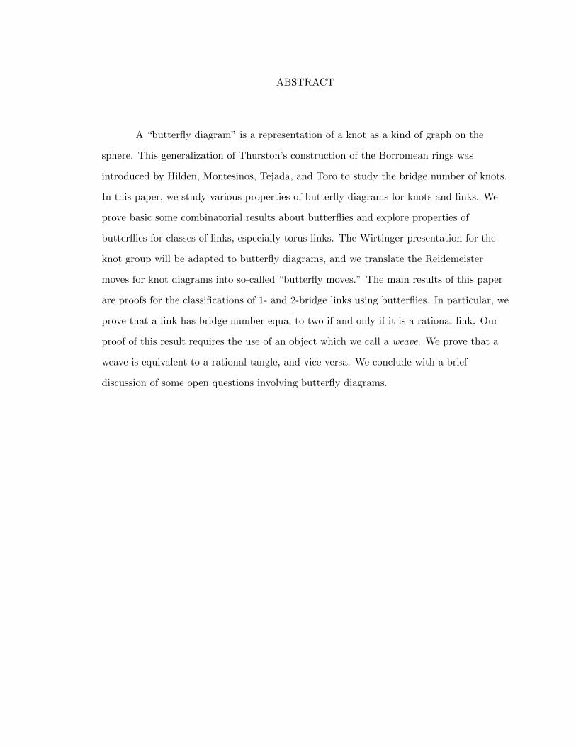
ABSTRACT
A “butterfly diagram” is a representation of a knot as a kind of graph on the
sphere. This generalization of Thurston’s construction of the Borromean rings was
introduced by Hilden, Montesinos, Tejada, and Toro to study the bridge number of knots.
In this paper, we study various properties of butterfly diagrams for knots and links. We
prove basic some combinatorial results about butterflies and explore properties of
butterflies for classes of links, especially torus links. The Wirtinger presentation for the
knot group will be adapted to butterfly diagrams, and we translate the Reidemeister
moves for knot diagrams into so-called “butterfly moves.” The main results of this paper
are proofs for the classifications of 1- and 2-bridge links using butterflies. In particular, we
prove that a link has bridge number equal to two if and only if it is a rational link. Our
proof of this result requires the use of an object which we call a weave. We prove that a
weave is equivalent to a rational tangle, and vice-versa. We conclude with a brief
discussion of some open questions involving butterfly diagrams.
A SURVEY OF BUTTERFLY DIAGRAMS FOR KNOTS AND LINKS
A ThesisSubmitted
in Partial Fulfillmentof the Requirement for the Degree
Master of Arts
Mark RonnenbergUniversity of Northern Iowa
May 2017

ii
This Study by: Mark Ronnenberg
Entitled: A SURVEY OF BUTTERFLY DIAGRAMS FOR KNOTS AND LINKS
Has been approved as meeting the thesis requirement for the
Degree of Master of Arts.
Date Dr. Theron Hitchman, Chair, Thesis Committee
Date Dr. Olena Ostapyuk, Thesis Committee Member
Date Dr. Bill Wood, Thesis Committee Member
Date Dr. Kavita Dhanwada, Dean, Graduate College

iii
To my parents, Douglas and Mary Ronnenberg. Without your unwavering
support, I would never have gotten this far.

iv
ACKNOWLEDGEMENTS
I would like to thank Dr. Bill Wood, for reviewing this paper as a member of my
committee, and for fostering my curiosity in his geometry courses. These courses were
some of the most enjoyable I have taken at UNI.
I would like to thank Dr. Olena Ostapyuk, for serving on my thesis committee,
but most importantly for being my first true mentor. Dr. Ostapyuk took a chance on me
by agreeing to work with me on my first research project. While I clearly had no idea
what I was getting myself into, her patience and guidance encouraged me to persevere.
Given our research and all of the courses I have taken under her, it is safe to say that no
one has influenced the mathematician I am now as much as she has.
I would like to thank Dr. Adrienne Stanley, for introducing me to the fascinating
world of abstract mathematics via set theory and topology. Dr. Stanley has gone out her
way to create opportunities for me, and others, to grow as mathematicians, and for that I
am forever grateful. In addition, she introduced me to the game Set, which has provided
relief from the stresses of academics so many times.
I owe a special thanks to Latricia Hylton, of the Academic Learning Center at UNI,
and to Dr. Douglas Mupasiri, head of the math department at UNI. Latricia has been the
most caring and supportive supervisor I have ever had in any position, and she has made
the past three and a half years at the ALC memorable in so many ways. Dr. Mupasiri’s
unwavering cheerfulness and passion for mathematics have been inspiring to me, especially
when the demands of graduate school have seemed daunting, which they often do.
Perhaps most of all, I would like to thank Dr. Theron Hitchman, my thesis adviser
and chair of my committee, for spending so much time with me doing mathematics, and
for pushing me to be a better mathematician and person. These past two years learning
topology under him (even if he isn’t a real topologist!) have confirmed my ambitions of
being a mathematician. His zest for mathematics, and life in general, have inspired me to
press on, no matter what challenges may lie ahead.
Finally, I would like to thank my parents, Douglas and Mary Ronnenberg, and my

v
fiance, Brittany Rinehart, for their unending care and support. I owe so much of my
success to them.

vi
TABLE OF CONTENTS
LIST OF FIGURES . . . . . . . . . . . . . . . . . . . . . . . . . . . . . . . . . . . . . . . . . . . . . . . . . . . . . . . . . . . . . . . . . . vii
CHAPTER 1. INTRODUCTION . . . . . . . . . . . . . . . . . . . . . . . . . . . . . . . . . . . . . . . . . . . . . . . . . . . . 1
CHAPTER 2. KNOTS AND LINKS. . . . . . . . . . . . . . . . . . . . . . . . . . . . . . . . . . . . . . . . . . . . . . . . . 3
CHAPTER 3. BUTTERFLY DIAGRAMS FOR LINKS . . . . . . . . . . . . . . . . . . . . . . . . . . . . . 8
CHAPTER 4. BUTTERFLIES FOR CLASSES OF LINKS . . . . . . . . . . . . . . . . . . . . . . . . . . 20
CHAPTER 5. KNOT GROUPS AND BUTTERFLIES . . . . . . . . . . . . . . . . . . . . . . . . . . . . . . 27
CHAPTER 6. BUTTERFLY MOVES AND REIDEMEISTER’S THEOREM . . . . . . . . 37
CHAPTER 7. CLASSIFICATION OF 1-BUTTERFLIES . . . . . . . . . . . . . . . . . . . . . . . . . . . . 47
CHAPTER 8. RATIONAL TANGLES AND WEAVES . . . . . . . . . . . . . . . . . . . . . . . . . . . . . . 56
CHAPTER 9. 2-BUTTERFLIES AND RATIONAL LINKS . . . . . . . . . . . . . . . . . . . . . . . . . 78
CHAPTER 10. FUTURE QUESTIONS . . . . . . . . . . . . . . . . . . . . . . . . . . . . . . . . . . . . . . . . . . . . . . 90
BIBLIOGRAPHY . . . . . . . . . . . . . . . . . . . . . . . . . . . . . . . . . . . . . . . . . . . . . . . . . . . . . . . . . . . . . . . . . . . . 92
vii
LIST OF FIGURES
2.1 Regular projection of a trefoil . . . . . . . . . . . . . . . . . . . . . . . . . . 5
2.2 Knot diagram of a trefoil . . . . . . . . . . . . . . . . . . . . . . . . . . . . 5
2.3 Knot diagram of a trefoil, which is equivalent to the diagram in Figure 2.2. 6
2.4 Reidemeister moves . . . . . . . . . . . . . . . . . . . . . . . . . . . . . . . . 7
3.1 A 3-butterfly for the trefoil. . . . . . . . . . . . . . . . . . . . . . . . . . . . 11
3.2 A butterfly with edges which must be double-counted. . . . . . . . . . . . . 12
3.3 Butterfly-link algorithm on a 3-butterfly for the trefoil. . . . . . . . . . . . . 13
3.4 Applying the link-butterfly algorithm to a trefoil. . . . . . . . . . . . . . . . 14
3.5 Simple butterfly. . . . . . . . . . . . . . . . . . . . . . . . . . . . . . . . . . 16
3.6 Constructing a butterfly on `. . . . . . . . . . . . . . . . . . . . . . . . . . . 17
4.1 Some examples of torus link diagrams . . . . . . . . . . . . . . . . . . . . . 20
4.2 Obtaining a canonical butterfly diagram for the (2, 3)-torus knot from its
canonical knot diagram. . . . . . . . . . . . . . . . . . . . . . . . . . . . . . 21
4.3 Canonical butterfly diagram for a (3,-5)-torus link. . . . . . . . . . . . . . . 22
4.4 Canonical butterfly diagarm for a (p, q)-torus link, with graph arcs labeled. 24
4.5 The twist knot T2. . . . . . . . . . . . . . . . . . . . . . . . . . . . . . . . . 25
4.6 Canonical butterfly diagrams for twist knots. . . . . . . . . . . . . . . . . . 25
5.1 Obtaining relations for the Wirtinger presentation. . . . . . . . . . . . . . . 28
5.2 Oriented knot diagram for a trefoil. Crossings and strands are labeled for
the Wirtinger presenation. . . . . . . . . . . . . . . . . . . . . . . . . . . . . 29
5.3 Obtaining relations for the Wirtinger presentation from a butterfly diagram. 30
5.4 Obtaining a relation for a presentation of G(K) from the equivalence class of
ai under '. . . . . . . . . . . . . . . . . . . . . . . . . . . . . . . . . . . . . 31
viii
5.5 Oriented (3,2)-torus knot butterfly diagram, labeled for the Wirtinger pre-
sentation. . . . . . . . . . . . . . . . . . . . . . . . . . . . . . . . . . . . . . 33
5.6 Oriented (p, q)-torus link butterfly diagram. . . . . . . . . . . . . . . . . . . 35
6.1 Canonical butterfly for a (3,2)-torus knot. . . . . . . . . . . . . . . . . . . . 37
6.2 Type I Reidemeister move. . . . . . . . . . . . . . . . . . . . . . . . . . . . 38
6.3 Type I butterfly move. . . . . . . . . . . . . . . . . . . . . . . . . . . . . . . 38
6.4 Type II Reidemeister move. . . . . . . . . . . . . . . . . . . . . . . . . . . . 40
6.5 Type II butterfly move. . . . . . . . . . . . . . . . . . . . . . . . . . . . . . 40
6.6 Determining which edges are connected to b′2 and b′′2, respectively. . . . . . . 41
6.7 Type III Reidemeister move. . . . . . . . . . . . . . . . . . . . . . . . . . . 43
6.8 Type III butterfly move. . . . . . . . . . . . . . . . . . . . . . . . . . . . . . 43
6.9 Performing a sequence of Reidemeister moves on T2. . . . . . . . . . . . . . 44
6.10 Performing a sequence of butterfly moves on a butterfly diagram for T2, which
is analogous to the moves in Figure 6.9. . . . . . . . . . . . . . . . . . . . . 45
7.1 A 1-butterfly diagram cannot have four sides. . . . . . . . . . . . . . . . . . 49
7.2 8-sided 1-butterfly diagrams. The corresponding knot diagrams are mirror
images of each other, and are the unknot. . . . . . . . . . . . . . . . . . . . 49
7.3 x is an A-vertex and y is an E-vertex. . . . . . . . . . . . . . . . . . . . . . 51
7.4 After inverse trunk-reducing move is applied to y, and then applying a Type
I butterfly move. . . . . . . . . . . . . . . . . . . . . . . . . . . . . . . . . . 52
7.5 BL if both y and z are A-vertices. . . . . . . . . . . . . . . . . . . . . . . . . 52
7.6 After applying inverse trunk-reducing moves to all E-vertices of BL, and the
result of a Type II butterfly move. . . . . . . . . . . . . . . . . . . . . . . . 53
7.7 After applying inverse trunk-reducing moves to all E-vertices of BL. . . . . 54
7.8 After applying inverse trunk-reducing moves to all E-vertices of BL. . . . . 54
8.1 Tangle sum. . . . . . . . . . . . . . . . . . . . . . . . . . . . . . . . . . . . . 57
8.2 Tangle product. . . . . . . . . . . . . . . . . . . . . . . . . . . . . . . . . . . 57

ix
8.3 Examples of integer tangles. . . . . . . . . . . . . . . . . . . . . . . . . . . . 58
8.4 Examples of reciprocal tangles. . . . . . . . . . . . . . . . . . . . . . . . . . 58
8.5 Examples of weave diagrams. . . . . . . . . . . . . . . . . . . . . . . . . . . 62
8.6 Performing an un-weaving step on a (5, 2)-weave. . . . . . . . . . . . . . . . 64
8.7 Performing an un-weaving step on a (5,-2)-weave. . . . . . . . . . . . . . . . 65
8.8 (2, 1)-weave, which is equivalent to the integer tangle [1]. . . . . . . . . . . . 67
8.9 Performing a weaving step on a (5, 2)-weave, plus an additional crossing. . . 73
8.10 Performing a weaving step on a (5,-2)-weave. . . . . . . . . . . . . . . . . . 74
9.1 Numerator and denominator closures of a rational tangle T . . . . . . . . . . 78
9.2 2-butterfly with a univalent B-vertex. . . . . . . . . . . . . . . . . . . . . . 80
9.3 This is not a 2-butterfly, since the trunks have coincident endpoints. . . . . 81
9.4 2-butterfly diagram representing the Hopf Link. . . . . . . . . . . . . . . . . 82
9.5 (7, 3) 2-butterfly diagram. . . . . . . . . . . . . . . . . . . . . . . . . . . . . 83
9.6 A (p, q) 2-butterfly with its vertices labeled modulo 4p. . . . . . . . . . . . . 84
9.7 A (p, q) 2-butterfly, with A- and E-vertices labeled modulo 2p. . . . . . . . 84
9.8 Turning a 2-butterfly into a weave. . . . . . . . . . . . . . . . . . . . . . . . 86
9.9 Flattening the sphere, giving the numerator closure of w(5, 2) + [1]. . . . . . 87

1
CHAPTER 1
INTRODUCTION
In 2012, Hilden, Montesinos, Tejada and Toro (HMTT) introduced the concept of
a butterfly as a way to represent knots and links [3]. Their idea is to generalize Thurston’s
construction of the Borromean Rings [10]. Thurston’s construction is achieved selecting
six line segments, one on each face of a cube, which cut each face in half. We then glue
the faces of the cube together in a particular way. The result of the gluing is a copy of the
3-dimensional sphere S3, with a link embedded within it.
Notice that the cube is homeomorphic to S2. Thus HMTT construct their
butterflies out of graphs embedded on S2, which divide S2 into polygonal faces. We select
special arcs on each of these faces, which we will call trunks. When we glue the faces in a
particular way, “folding” along the trunks, the result is a copy of S3 with a link embedded
within it.
HMTT developed the concept of butterflies in hopes of generalizing the
classification of 2-bridge links to 3-bridge links. They lay the groundwork for this endeavor
in [4]. We believe that to gain insight into this problem, it will be useful to reconstruct the
classification of 2-bridge links using butterflies. This is the main thrust of this paper.
In Chapter 2 we review basic notions about knots and links. In Chapter 3, we will
define precisely what a butterfly is, as defined by HMTT. We will alter their definition
slightly for this paper. This altered definition will simplify some of the arguments we
make throughout this paper. Toward the end of Chapter 3, we will prove some basic
results about butterflies, including a method for determining the crossing number of a
knot diagram from a butterfly diagram.
Chapter 4 will introduce some examples of butterflies, including a treatment of
butterflies for torus links. In Chapter 5, we will discuss knot groups as they relate to
butterflies. In particular, we will adapt the Wirtinger presentation for knot groups to
butterflies, and derive a simplified method from this adaptation. We will use this
2
simplified method to derive the well-known presentation of the knot group for torus links
using butterflies.
An open problem, posed by HMTT, is to find a complete set of “butterfly moves”
to transform a given butterfly diagram into an equivalent one. In Chapter 6, we develop
butterfly moves which are analogous to the traditional Reidemeister moves for knot
diagrams. At the end of the chapter, we prove that these butterfly moves, along with the
trunk-reducing move introduced by HMTT, is enough to determine equivalence of
butterfly diagrams.
The remaining chapters focus on the classification of links by bridge number. In
particular, we reconstruct the classifications of 1- and 2-bridge links using butterflies. In
Chapter 7, we show that every 1-butterfly corresponds to the unknot. Chapter 8 begins
with a review of the theory of rational tangles. We then introduce a new object, which we
call a weave. At the end of the chapter, we will prove the every weave is a rational tangle,
and vice-versa.
The main result of this paper is proved in Chapter 9. We prove that any
2-butterfly corresponds to a rational link, and that any rational link has a 2-butterfly.
Thus we construct a new proof that any 2-bridge link is a rational link, and vice-versa.
We conclude this paper with a brief discussion of further questions in Chapter 10.

3
CHAPTER 2
KNOTS AND LINKS
This chapter will introduce basic ideas and notations needed throughout the rest
of this paper. For comprehensive discussions of these topics and more, see [1].
A knot can be considered as an embedding of a circle S1 into S3. Here, we let S3
the 3-dimensional sphere, or the one point compactification of R3. By an embedding, we
mean a map f : S1 → f(S1) ⊂ S3, which is a homeomorphism. We will consider a knot as
an equivalence class of embeddings of a circle. The equivalence relation between knots will
be ambient isotopy.
Definition 2.1. (Isotopy) Two embeddings f0, f1 : S1 → S3 are said to be isotopic if there
exists an embedding F : S1 × I → S3 × I such that F (x, t) = (f(x, t), t), x ∈ S1,
t ∈ I = [0, 1], and f(x, 0) = f0(x), f(x, 1) = f1(x).
The mapping F is called a level-preserving isotopy connecting f0 to f1.
It can be shown that any two embeddings S1 → S3 are isotopic [1]. Thus the
notion of isotopy is not strong enough to differentiate between different knots.
Definition 2.2. (Ambient Isotopy) Two embeddings f0, f1 : S1 → S3 are said to be
ambient isotopic if there is a level-preserving isotopy H : S3 × I → S3 × I, with
H(x, t) = (ht(x), t), such that f1 = h1f0 and f0 is the identity map on S3. The mapping
H is called an ambient isotopy.
The notion of ambient isotopy is closer to what we seek. However, some strange
cases are allowed by our definition of embedding, known as wild knots [1]. We do not want
to consider wild knots in our study. We will only consider tame knots, that is, knots which
are ambient isotopic to a simple closed polygon in S3. To ensure that we will only have to
deal with tame knots, we will restrict our maps to the piecewise linear category. Thus we
restrict our definitions of embeddings and isotopies to be piecewise linear.

4
We can now state our definition for a knot. We shall consider a knot to be a
piecewise linear ambient isotopy equivalence class of piecewise linear embeddings S1 → S3.
Definition 2.3. (Knot Equivalence) Two piecewise linear knots are equivalent if they are
piecewise linear ambient isotopic.
A piecewise linear embedding of a finite disjoint union of circles into S3 is called a
link. If a link is an embedding of n circles, then it is an n-component link. A knot is a link
with one component. Often we will use the terms “knot” and “link” interchangeably.
When we really mean knot, and not link, or vice-versa, we shall say so. From now on we
will assume that we are working within the piecewise linear category. Thus we will omit
the phrase “piecewise linear.”
It will often be convenient to consider projections of knots onto a plane in R3.
Instead of considering a knot as an embedding in S3, we may consider it in R3 via
stereographic projection. Thus a knot K is a simple closed polygon in R3. Let p : R3 → E
be an orthogonal projection of R3 onto the plane E. A point P ∈ p(K) ⊂ E whose
preimage p−1(P ) contains more than one point of K is called a multiple point.
Definition 2.4. (Regular Projection) A projection p of a knot K is called regular if
(i) There are only finitely many multiple points, and each multiple point is a double
point, that is, it has exactly two points in its preimage.
(ii) No vertex of K is mapped onto a multiple point.
For example, Figure 2.1 is a regular projection of a trefoil knot.
A regular projection is not enough to uniquely determine a knot. We need to
include more information. Imagine looking down onto a knot from the projection point for
a regular projection. Some of the arcs cross over other arcs. The arcs which go over are
called overpasses, and the arcs which go under are called underpasses. If in a regular
projection we indicate which arc is the overpass and which arc is the underpass at each
double point, by breaking the underpass, then the knot can be recovered. We will refer to

5
Figure 2.1: Regular projection of a trefoil
such a regular projection as a knot diagram. If orientation is also indicated, we will call
such a projection an oriented knot diagram. In a knot diagram, double points will be
called crossings. Figure 2.2 is a knot diagram for the trefoil, obtained from the regular
projection in Figure 2.1.
Figure 2.2: Knot diagram of a trefoil
Definition 2.5. (Equivalence of Knot Diagrams) We say that two knot digrams are
equivalent if they represent the same knot.
We note that if two knot diagrams are related via a planar isotopy, that is, a
continuous deformation in E which does not change any of the crossings of a diagram,

6
then they are equivalent. This allows to draw knot diagrams with smooth curves, such as
in Figure 2.3. This knot diagram corresponds to a trefoil, and is equivalent to the diagram
in Figure 2.2. However, two equivalent knot diagrams may not in general be related by
planar isotopy.
Figure 2.3: Knot diagram of a trefoil, which is equivalent to the diagram in Figure 2.2.
By a theorem of Reidemeister, there is another way to determine when two knot
diagrams are equivalent. Consider the Reidemeister moves depicted in Figure 2.4. These
are simple moves performed on a knot diagram which do not alter the topology of the
corresponding knot. By Reidemeister’s Theorem, the Reidemeister moves are enough to
determine, up to ambient isotopy, whether two knot diagrams are equivalent.
Theorem 2.6. (Reidemeister’s Theorem) Let D and D′ be two knot diagrams. Then D
and D′ are equivalent if and only if they are related be a finite sequence of Reidemeister
moves and planar isotopies.

7
(a) Type I move (b) Type II move
(c) Type III move
Figure 2.4: Reidemeister moves
8
CHAPTER 3
BUTTERFLY DIAGRAMS FOR LINKS
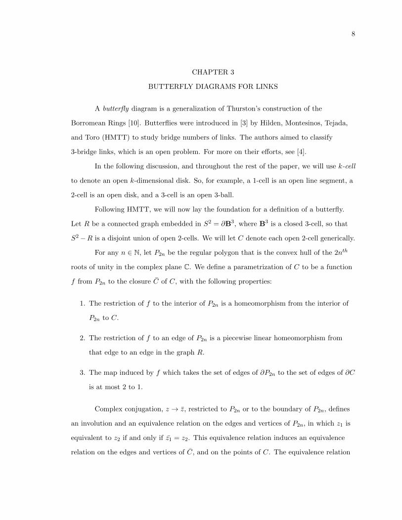
A butterfly diagram is a generalization of Thurston’s construction of the
Borromean Rings [10]. Butterflies were introduced in [3] by Hilden, Montesinos, Tejada,
and Toro (HMTT) to study bridge numbers of links. The authors aimed to classify
3-bridge links, which is an open problem. For more on their efforts, see [4].
In the following discussion, and throughout the rest of the paper, we will use k-cell
to denote an open k-dimensional disk. So, for example, a 1-cell is an open line segment, a
2-cell is an open disk, and a 3-cell is an open 3-ball.
Following HMTT, we will now lay the foundation for a definition of a butterfly.
Let R be a connected graph embedded in S2 = ∂B3, where B3 is a closed 3-cell, so that
S2−R is a disjoint union of open 2-cells. We will let C denote each open 2-cell generically.
For any n ∈ N, let P2n be the regular polygon that is the convex hull of the 2nth
roots of unity in the complex plane C. We define a parametrization of C to be a function
f from P2n to the closure C of C, with the following properties:
1. The restriction of f to the interior of P2n is a homeomorphism from the interior of
P2n to C.
2. The restriction of f to an edge of P2n is a piecewise linear homeomorphism from
that edge to an edge in the graph R.
3. The map induced by f which takes the set of edges of ∂P2n to the set of edges of ∂C
is at most 2 to 1.
Complex conjugation, z → z, restricted to P2n or to the boundary of P2n, defines
an involution and an equivalence relation on the edges and vertices of P2n, in which z1 is
equivalent to z2 if and only if z1 = z2. This equivalence relation induces an equivalence
relation on the edges and vertices of C, and on the points of C. The equivalence relation

9
on C induces an equivalence relation on S2 = ∂B3. We denote the equivalence relation on
a 2-cell C by ∼. We denote the equivalence relation on S2 = B3, which is generated by
the relations ∼, by '. Then for all x and y in S2, x ' y if and only if there exists a finite
sequence x = x1, . . ., xl = y with xi ∼ xi+1 for i = 1, . . ., l − 1.
Each P2n contains the line segment [−1, 1], which is the fixed point set of z → z
restricted to P2n. The image of this line segment, fC([−1, 1]), is called the trunk t of C. A
pair, (C, t), is called a butterfly with trunk t. The wings W and W ′ are just fC(P2n∩ upper
half plane) and fC(P2n∩ lower half plane), and W ∩W ′ = t. We denote by T the
collection of all trunks t over all C.
Let us denote by M(R, T ) the space B3/ ' with the topology of the identification
map p : B3 →M(R, T ), where ' is the minimal equivalence relation generated by the
equivalence relation ' defined on S2.
Equivalence classes of points of C, under ∼, contain two points except for those
points in f([−1, 1]), where there is only one point. If x is a vertex of R, its equivalence
class under the equivalence relation ', on S2 = B3, is composed entirely of vertices of R.
We classify the vertices as follows: A member of R ∩ T will be called an A-vertex. A
member of p−1(p(v)), v ∈ R ∩ T , which is not an A-vertex will be called an E-vertex. A
vertex of R which is neither an A-vertex nor an E-vertex will be called a B-vertex iff
p−1(p(v)) contains at least one non-bivalent vertex of R.
With these definitions in hand, we are ready to define an m-butterfly as HMTT do
in [3].
Definition 3.1. (HMTT m-butterfly) Let R and T be as above. For m ≥ 1, an
m-butterfly is a 3-ball B3 with m butterflies (Ci, ti), i = 1, . . ., m, on its boundary
S2 = ∂B3, such that R has only A-vertices, E-vertices, and B-vertices, each A-vertex and
each E-vertex is bivalent in R, and T has m components.
Now, for our purposes we wish to alter this definition slightly. First, we remove the
condition that a B-vertex is such that p−1(p(v)) contains a vertex which is non-bivalent.
Instead, we will allow a B-vertex to simply be a vertex which is neither an A-vertex nor an
10
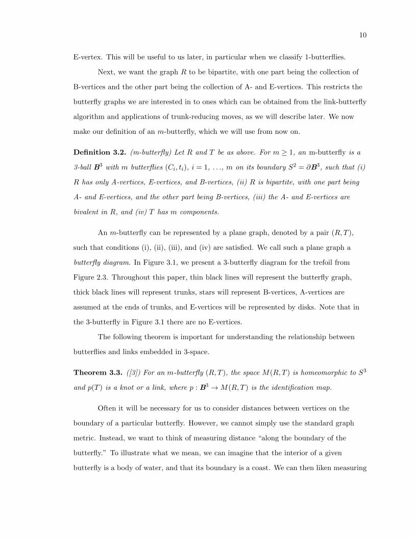
E-vertex. This will be useful to us later, in particular when we classify 1-butterflies.
Next, we want the graph R to be bipartite, with one part being the collection of
B-vertices and the other part being the collection of A- and E-vertices. This restricts the
butterfly graphs we are interested in to ones which can be obtained from the link-butterfly
algorithm and applications of trunk-reducing moves, as we will describe later. We now
make our definition of an m-butterfly, which we will use from now on.
Definition 3.2. (m-butterfly) Let R and T be as above. For m ≥ 1, an m-butterfly is a
3-ball B3 with m butterflies (Ci, ti), i = 1, . . ., m on its boundary S2 = ∂B3, such that (i)
R has only A-vertices, E-vertices, and B-vertices, (ii) R is bipartite, with one part being
A- and E-vertices, and the other part being B-vertices, (iii) the A- and E-vertices are
bivalent in R, and (iv) T has m components.
An m-butterfly can be represented by a plane graph, denoted by a pair (R, T ),
such that conditions (i), (ii), (iii), and (iv) are satisfied. We call such a plane graph a
butterfly diagram. In Figure 3.1, we present a 3-butterfly diagram for the trefoil from
Figure 2.3. Throughout this paper, thin black lines will represent the butterfly graph,
thick black lines will represent trunks, stars will represent B-vertices, A-vertices are
assumed at the ends of trunks, and E-vertices will be represented by disks. Note that in
the 3-butterfly in Figure 3.1 there are no E-vertices.
The following theorem is important for understanding the relationship between
butterflies and links embedded in 3-space.
Theorem 3.3. ([3]) For an m-butterfly (R, T ), the space M(R, T ) is homeomorphic to S3
and p(T ) is a knot or a link, where p : B3 →M(R, T ) is the identification map.
Often it will be necessary for us to consider distances between vertices on the
boundary of a particular butterfly. However, we cannot simply use the standard graph
metric. Instead, we want to think of measuring distance “along the boundary of the
butterfly.” To illustrate what we mean, we can imagine that the interior of a given
butterfly is a body of water, and that its boundary is a coast. We can then liken measuring

11
Figure 3.1: A 3-butterfly for the trefoil.
distance from two points on the boundary of the butterfly to measuring the length of the
shoreline between them, which we do by counting graph edges. Consider, for example, the
butterfly in Figure 3.2. Sticking with our water and coast analogy, we can measure the
distance from α to β, traveling counterclockwise. If we imagine we are swimming from α
to β, while remaining very close to the shoreline the entire time, the we must travel
around the two edges which contain γ as an endpoint. In fact, in counting edges to
measure distance, we will count these two edges twice. Thus the distance measured from
α to β, traveling counterclockwise, is six. In fact, if we measure the distance from α to β
clockwise, the distance is also six. In general, we should expect to obtain different values
depending on whether we measured distance clockwise or counterclockwise.
Measuring distance in this way has the peculiar feature that we do not always
obtain a value of zero when measuring distance from a vertex to itself. This is because in

12
some cases it matters which “side” of a vertex we begin measuring from. For example,
consider the vertex γ in Figure 3.2. We can measure the distance from γ to itself,
beginning on the “trunk side,” and traveling clockwise, to be equal to two. Note that we
count the edge connecting γ to the univalent B-vertex twice.
When we measure distance as described above, we refer to it as butterfly boundary
distance.
α
β
γ
Figure 3.2: A butterfly with edges which must be double-counted.
Definition 3.4. (t-equivalence) Let t be the trunk of a butterfly B. Let a be an A-vertex
of t. If two vertices α and α′ of B are equidistant from a, on the “trunk side” of a, in
butterfly boundary distance, then we say that α and α′ are t-equivalent.
Remark 3.5. Note that if α and α′ are t-equivalent, then α ∼ α′, where ∼ is the
equivalence relation on the butterfly containing t, as defined previously in this chapter.
We will now describe a practical algorithm for obtaining a knot diagram from a
given butterfly diagram. This algorithm is referred to as the butterfly-link algorithm [3].
Consider an m-butterfly (R, T ) which represents the knot K. For each t ∈ T we perform
the following steps. Identify t-equivalent pairs of A- or E-vertices on the boundary of the
butterfly containing t. For each pair, draw an arc connecting the vertices which crosses t
exactly once and never leaves the butterfly containing t. These are the arcs of the link

13
which are obtained from the quotient map p : B3 →M(R, T ). Consider a vertical line
segment in P2n, which connects two vertices of ∂P2n. Then each arc we draw corresponds
to the image of such a vertical line under p. These arcs will pass under the trunks in the
resulting link diagram. The newly constructed arcs, together with the trunks, will make
up a knot diagram for K. See [3] for details. Figure 3.3 shows the results of the
butterfly-link algorithm on the 3-butterfly in Figure 3.1. The dotted lines represents the
arcs drawn in the algorithm, which are under-arcs in the resulting diagram. The resulting
diagram is equivalent to the trefoil diagram from Figure 2.3.
Figure 3.3: Butterfly-link algorithm on a 3-butterfly for the trefoil.
It is also possible to obtain a butterfly diagram from a given knot diagram. This
process shall be called the link-butterfly algorithm. The link-butterfly algorithm is
described in proving the following theorem, due to HMTT.
Theorem 3.6. (Link-Butterfly Algorithm [3]) Every knot or link can be represented by an
14
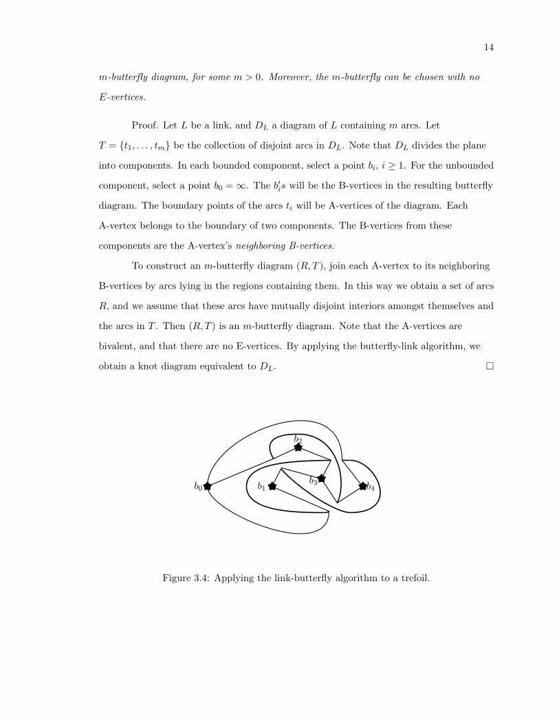
m-butterfly diagram, for some m > 0. Moreover, the m-butterfly can be chosen with no
E-vertices.
Proof. Let L be a link, and DL a diagram of L containing m arcs. Let
T = {t1, . . . , tm} be the collection of disjoint arcs in DL. Note that DL divides the plane
into components. In each bounded component, select a point bi, i ≥ 1. For the unbounded
component, select a point b0 =∞. The b′is will be the B-vertices in the resulting butterfly
diagram. The boundary points of the arcs ti will be A-vertices of the diagram. Each
A-vertex belongs to the boundary of two components. The B-vertices from these
components are the A-vertex’s neighboring B-vertices.
To construct an m-butterfly diagram (R, T ), join each A-vertex to its neighboring
B-vertices by arcs lying in the regions containing them. In this way we obtain a set of arcs
R, and we assume that these arcs have mutually disjoint interiors amongst themselves and
the arcs in T . Then (R, T ) is an m-butterfly diagram. Note that the A-vertices are
bivalent, and that there are no E-vertices. By applying the butterfly-link algorithm, we
obtain a knot diagram equivalent to DL. �
b3b0
b2
b4b1
Figure 3.4: Applying the link-butterfly algorithm to a trefoil.

15
Consider a knot diagram D. An arc of D which is an overpass (that is, an arc
which has an under-crossing) is called a bridge of D. We define a maximal bridge of D to
be a bridge which is not contained in another bridge which has more under-crossings.
Note that if an arc has no under-crossings at all, then we do not consider it as a bridge
(nor as a maximal bridge). The bridge number of D is defined to be the number of
maximal bridges in D. We can define bridge number for links.
Definition 3.7. (Bridge Number) Let L be a link. We define the bridge number of L to be
the least bridge number over all diagrams of L. We denote the bridge number of L by b(L).
In a similar vein, HMTT define what they call the butterfly number of a link.
Definition 3.8. (Butterfly number) Let L be a link. The least m such that L has an
m-butterfly diagram is called the butterfly number of L. We denote the butterfly number
of L by m(L).
Theorem 3.9. ([3]) For any link L, the butterfly number of L is equal to the bridge
number of L.
As a consequence of Theorem 3.9, we can obtain results about the bridge number
of a link by studying its butterfly number. This fact is of great importance when we study
1- and 2-bridge links, and is a motivating factor for HMTT’s study of 3-butterflies in an
attempt to classify 3-bridge links.
In their proof of Theorem 3.9, HMTT utilize what they call a trunk-reducing
move. Let L be a link and D = (R, T ) an m-butterfly diagram of L obtained from the
link-butterfly algorithm. Recall that D has no E-vertices. In fact, D will consist of only
two types of butterflies. The butterflies which come from overpasses will have more than
two A-vertices, while the trunks coming from underpasses will have exactly two
A-vertices. The latter type of butterfly will be called a simple butterfly. Simple butterflies
have four sides, see Figure 3.5. A trunk-reducing move allows us to replace a simple
butterfly in D with an E-vertex. We have the following theorem.

16
Figure 3.5: Simple butterfly.
Theorem 3.10. ([3]) A trunk-reducing move converts an m-butterfly diagram of a link L
into an (m− 1)-butterfly diagram of the same link L. The new diagram gets a new
E-vertex in place of a simple butterfly.
For details and proofs of Theorem 3.9 and Theorem 3.10, see [3]. A trunk-reducing
move turns a given butterfly diagram into a different diagram of the same link. The
notion of a link having more than one butterfly diagram is very important, and is
analogous to the fact that a link has infinitely many knot diagrams. From this notion we
can define equivalence of butterfly diagrams.
Definition 3.11. (Equivalence of butterfly diagrams) Two butterfly diagrams are said to
be equivalent if they represent the same link.
With the basic theory of butterflies laid out, we proceed to prove some simple
combinatorial theorems about butterfly diagrams.
Theorem 3.12. Let L be a link, and D a knot diagram of L, and B a butterfly diagram
for L obtained from D by the link-butterfly algorithm. Let ` be an overpass of D. Then `
has n underpasses if and only if the butterfly corresponding to ` has 4(n+ 1) sides.
Proof. First suppose ` has n underpasses. Apply the link-butterfly algorithm on D
to obtain B. In Figure 3.6 we show the application of the algorithm locally about `. Recall
that in measuring butterfly boundary distance, we do so by traveling along the boundary
of a butterfly in some consistent orientation, and that we may have to double-count some
edges. With this in mind, it can be shown that each underpass of ` will contribute four
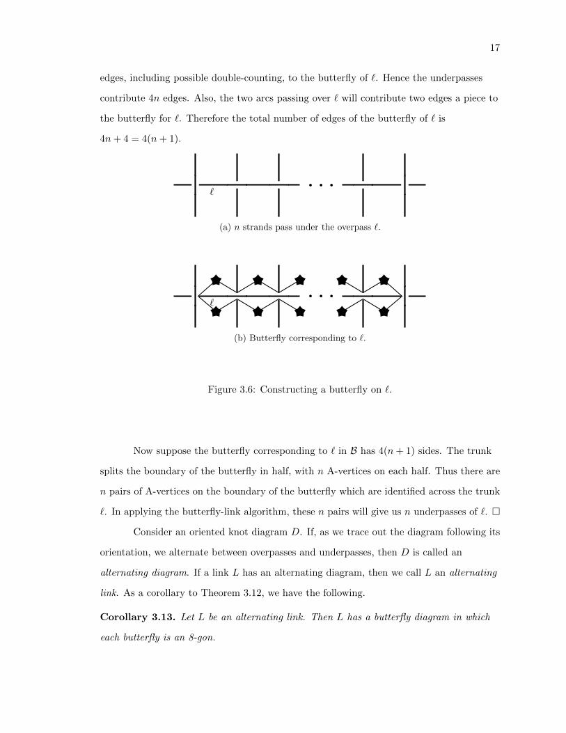
17
edges, including possible double-counting, to the butterfly of `. Hence the underpasses
contribute 4n edges. Also, the two arcs passing over ` will contribute two edges a piece to
the butterfly for `. Therefore the total number of edges of the butterfly of ` is
4n+ 4 = 4(n+ 1).
`
(a) n strands pass under the overpass `.
`
(b) Butterfly corresponding to `.
Figure 3.6: Constructing a butterfly on `.
Now suppose the butterfly corresponding to ` in B has 4(n+ 1) sides. The trunk
splits the boundary of the butterfly in half, with n A-vertices on each half. Thus there are
n pairs of A-vertices on the boundary of the butterfly which are identified across the trunk
`. In applying the butterfly-link algorithm, these n pairs will give us n underpasses of `. �
Consider an oriented knot diagram D. If, as we trace out the diagram following its
orientation, we alternate between overpasses and underpasses, then D is called an
alternating diagram. If a link L has an alternating diagram, then we call L an alternating
link. As a corollary to Theorem 3.12, we have the following.
Corollary 3.13. Let L be an alternating link. Then L has a butterfly diagram in which
each butterfly is an 8-gon.

18
Proof. Since L is alternating, it has an alternating knot diagram. In this diagram,
each overpass has exactly one underpass. Apply the link-butterfly algorithm. By Theorem
3.12, each butterfly will have 4(1 + 1) = 8 sides. �
Let D be a knot diagram. We define the crossing number of D to be the number
of crossings in D. Similarly to our definition of the bridge number of a link, we can define
the crossing number of a link as follows.
Definition 3.14. (Crossing Number) Let L be a link. We define the crossing number of L
to be the least crossing number among all knot diagrams of L. We denote the crossing
number of L by cr(L).
Our next theorem gives us a way to determine crossing numbers from butterflies.
Theorem 3.15. Let L be a link and B a butterfly diagram of L. Let a and e be the
number of A-vertices and E-vertices of B, respectively. Then the crossing number of the
link diagram corresponding to B is a2 + e.
Proof. Expand each E-vertex of B into a simple butterfly via inverse
trunk-reducing moves. Note that each simple butterfly contains exactly two A-vertices.
Let n be the number of A-vertices in the resulting butterfly diagram. Let D be the link
diagram corresponding to B via the butterfly-link algorithm. The identification of two
A-vertices across a trunk corresponds to a crossing in D. Thus D has n2 crossings. Now we
return to the original butterfly diagram B by performing trunk-reducing moves on each of
the simple butterflies we obtained earlier. Since there were e E-vertices in B, we will
perform e trunk-reducing moves. Each move eliminates two A-vertices. So the number of
A-vertices in B is given by a = n− 2e = 2(n2 − e). It follows that n2 = a
2 + e. Since neither
a trunk-reducing move nor its inverse alters the link diagram D, we conclude that the
crossing number of D is given by a2 + e. �
As an immediate corollary, it is possible to compute the crossing number of a link
from its butterfly diagrams.

19
Corollary 3.16. Let L be a link. For a butterfly diagram of L, let a and e be the number
of A-vertices and E-vertices, respectively. Then cr(L) is the least value of a2 + e taken over
all butterfly diagrams of L.

20
CHAPTER 4
BUTTERFLIES FOR CLASSES OF LINKS
In this section we present descriptions for butterflies of some important classes of
links. We begin with a study of torus links. A torus link is a link which can be embedded
on a torus without self-intersection. A familiar example is the trefoil knot of Figure 2.3.
In particular, we will now describe a construction for a (p, q)-torus link, where p and q are
integers and p > 0. Construct p horizontal parallel strands. For q > 0, the bottom most q
strands are wrapped up and over the remaining strands, one at a time. For q < 0, the
upper most q strands are wrapped down and over the remaining strands, one at a time.
Once the wrapping is complete, close off the strands so that no new crossings are created.
See Figure 4.1 for some examples.
(3, 2) (2,−5)
Figure 4.1: Some examples of torus link diagrams
From this canonical diagram, we can construct a canonical butterfly diagram for a
(p, q)-torus link. Our canonical butterfly diagram is obtained by applying the
link-butterfly algorithm to a canonical knot diagram. In applying the algorithm, the
B-vertex ∞ will be actually be taken as the north pole on S2 = ∂B3. In projecting S2
down to the plane, the B-vertex ∞ will really be the point at infinity of the plane. The
butterfly diagram obtained from the algorithm will likely contain simple butterflies. We
will replace these with E-vertices via trunk-reducing moves. The resulting butterfly
diagram will consist of |q| arcs, with endpoints at two B-vertices, one of which is b0 =∞

21
(since it lies in the unbounded component of the projection plane), the other we call b1.
These two B-vertices will each have degree |q|. Each arc of the graph will contain exactly
two A-vertices, and p− 2 E-vertices. The diagram will contain 2q + q(p− 2) = pq total A-
and E-vertices. For q > 0, the trunks will, moving from b1 toward ∞, start on an A-vertex
nearest to b1, and end on the A-vertex on the adjacent arc which is nearest to b0 =∞
(moving counterclockwise about b1). See Figure 4.2 and Figure 4.3.
(a)
b1
∞
∞
∞
(b)
∞
∞
∞b1
(c)
Figure 4.2: Obtaining a canonical butterfly diagram for the (2, 3)-torus knot from its canon-ical knot diagram.
With our canonical diagrams in hand, we cite a few useful results without proof.
The interested reader may find details in [7].
Theorem 4.1. Let L1 be a (p, q)-torus link.
(i) Suppose q > 0. Let L2 be a (q, p)-torus link. Then L1 is equivalent to L2.
(ii) Let L2 be a (p,−q)-torus link. Then L2 is the mirror image of L1.
Our canonical butterfly diagram for torus links allows us to give a new proof for a
basic result about torus links. First we prove the following lemma.

22
∞
∞
∞
∞
∞b1
Figure 4.3: Canonical butterfly diagram for a (3,-5)-torus link.
Lemma 4.2. Let L be a (p, q)-torus link and BL a canonical butterfly diagram for L. Let
a be an A-vertex of BL. Then the equivalence class of a, under the equivalence relation '
on S2 = B3, contains exactly p elements.
Proof. Without loss of generality, we may assume q > 0. For the case q < 0, a
similar argument will apply, the only difference being that we label trunks and vertices in
a counterclockwise fashion.
We label the trunks of BL as t0, t1, . . ., tq−1, going clockwise about the B-vertex
b1. Next we orient each trunk of BL, so that the corresponding link diagram is an oriented
diagram. In particular, we will orient each trunk as “moving away from” b1. For each
trunk ti, we denote by ai and a′i the incoming and outgoing A-vertices of ti, respectively.
In Figure 5.6, the omitted sections of each ray, represented by three dots, are the segments
containing the p− 2 E-vertices. We note that these sections contain 2(p− 2) edges.
Fix i ∈ {0, . . ., p− 1}. We will determine the size of the equivalence class of a′i. As

23
a result of the symmetric properties of BL, this will be sufficient to determine the size of
the equivalence class of any A-vertex of BL.
Note that the butterfly boundary distance of a′i to b1 is 2 + 2(p− 1) + 1 = 2p− 1.
Also note that a′i is ti+1-equivalent to some vertex e1, which is either an E-vertex or an
A-vertex. Since the butterfly boundary distance from b1 to a′i is 2p− 1, and the butterfly
boundary distance from b1 to ai+1 is 1, we obtain that the butterfly boundary distance
from b1 to e1 must be 2p− 1− 2 = 2p− 3.
Similarly, for some j, we have ej is ti+j+1-equivalent to ej+1, and that the butterfly
boundary distance from b1 to ej+1 is 2p− 1− 2(j + 1), where the trunk indices are taken
modulo q. Now, note that the equivalence class of a′i must contain another A-vertex.
Then for some ` we obtain e` = aj , for some j. In particular, note that the butterfly
boundary distance from b1 to aj is 1. Thus we want to find ` such that 2p− 1− 2` = 1.
But then we see that p = `. So the sequence a′i = e0, e1, e2, . . ., ep−2, ep−1 = aj is such
that the corresponding sequence of butterfly boundary distances to b1 is 2p− 1, 2p− 3,
2p− 5, . . ., 3, 1. Thus the equivalence class of a′i contains exactly p elements. �
Theorem 4.3. Let L be a (p, q)-torus link. Let d = gcd(p, q). Then L has d link
components.
Proof. Let BL be the canonical butterfly diagram for L. Without loss of generality,
suppose q > 0, since a similar argument applies if q < 0. Note that by Lemma 4.2, each
equivalence class of A- or E-vertices under ' contains exactly p elements.
We will count the components of L from BL. Let a0 be an A-vertex of B, which is
nearer to b0 =∞ than to b1 in butterfly boundary distance. Starting at the arc containing
a0, and traveling clockwise about b1, label the arcs in ascending order modulo q. Then the
arc containing a0 is labeled “0”. To trace out the component of L corresponding to a0’s
equivalence class, we do the following. Trace out the equivalence class of a0 clockwise from
a0. We will eventually reach an A-vertex. If it is on the trunk containing a0, we are done.
If not, then we move to the A-vertex on the other end of the trunk and trace out its
equivalence class in the same way. Eventually, we will end up at the trunk containing a0.

24
∞
∞
∞
∞
∞
0
1
2
3
q − 1
b1
a0
Figure 4.4: Canonical butterfly diagarm for a (p, q)-torus link, with graph arcs labeled.
When this happens, we will have traced out the component corresponding to a0.
Now, we would like to know how many trunks are in each component. Again, by
symmetry of BL, each component should contain the same number of trunks. In tracing
a0’s component, the process terminates when we arrive at an A-vertex lying on the arc
labeled “0”. Since each equivalence class of A- and E-vertices contains p elements, we can
find a positive integer ` such that p` ≡ 0 (mod q). In particular, let ` be least such that
this property holds. In other words, let p` = lcm(p, q). Thus there are ` trunks in each
component of L. There are q total trunks, so there are q/` components of L. Now recall
that p` = lcm(p, q) = pqd . It follows that ` = q
d , so q/` = d. Therefore L has d components.
�
The next class of knots we consider is the twist knots. Let n be a positive integer.
A twist knot of n half-twists, which we denote by Tn, is obtained by twisting two parallel

25
strands n times and closing them up so that the resulting knot is alternating. For
example, a knot diagram of T2 is depicted in Figure 4.5.
Figure 4.5: The twist knot T2.
∞b1
(a) General twist knot Tn. The squaresrepresent A-vertices. (b) The twist knot T2.
Figure 4.6: Canonical butterfly diagrams for twist knots.
By applying the link-algorithm to a twist knot Tn, we can obtain a canonical
butterfly diagram for twist knots. We present the canonical diagram in Figure 4.6a. The
shaded region of Figure 4.6a will contain n 8-sided butterflies “stacked on top of each
other.” They are to be constructed as follows. Construct n− 1 paths connecting the

26
B-vertices b0 =∞ and b1 which intersect only at their endpoints. Each of these paths will
contain four edges, including two A-vertices and one B-vertex. As a result, the B-vertices
∞ and b1 will each have degree n+ 1. There is only one way to place the trunks in the
resulting polygonal faces so that we obtain a proper (n+ 2)-butterfly diagram. The n
8-sided butterflies in the shaded region correspond to the n twists in the knot. For an
example of a canonical butterfly diagram for T2, see Figure 4.6b. We encourage the reader
to apply the butterfly-link algorithm to Figure 4.6b and to compare the result with the
knot diagram of T2 in Figure 4.5.

27
CHAPTER 5
KNOT GROUPS AND BUTTERFLIES
Recall that knots are embedded in S3 (or R3). It turns out that one can learn a lot
about a knot by studying its complement in S3. The famous Gordon-Luecke Theorem [2]
states that if two knots have complements which are orientation-preserving
homeomorphic, then the knots are isotopic, hence equivalent. This results does not hold
for links in general, so in this section we will restrict our attention to knots. A powerful
tool for studying knot complements is the fundamental group of the complement. The
fundamental group of a knot complement will be referred to as the knot group of a knot.
It is known that homeomorphic spaces have isomorphic fundamental groups. Thus
equivalent knots have isomorphic knot groups. Knot groups therefore are useful in
distinguishing distinct knots. In this section we will develop methods for computing knot
groups from butterflies based on the well-known Wirtinger presentation. The following
discussion of the Wirtinger presentation is based heavily on [1].
The Wirtinger presentation is a way to present a knot group via generators and
relations. We will describe the general method of the Wirtinger presentation, and then we
will develop the method for butterflies. To obtain a Wirtinger presentation for a given
knot, we will consider consider a knot diagram. We must put an orientation on the
diagram. Each strand of the diagram is assigned a label si. These will be the generators of
the knot group. The relations are obtained from the crossings of the diagram. Beginning
with the under-arc which is leaving the crossing, travel counterclockwise on a small circle
about the crossing, reading off the labels of the strands. The strands which are leaving the
crossing are assigned an exponent of −1, whereas the strands that are entering the
crossing are assigned an exponent of 1. In this way each crossing gives us a word in the
generators of the knot group, which is taken as a relation.
This method is summarized in the following theorem.
28
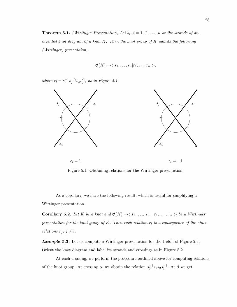
Theorem 5.1. (Wirtinger Presentation) Let si, i = 1, 2, . . ., n be the strands of an
oriented knot diagram of a knot K. Then the knot group of K admits the following
(Wirtinger) presentaion,
G(K) =< s1, . . . , sn|r1, . . . , rn >,
where ri = s−1i s−εij sksεij , as in Figure 5.1.
sisj
sk
sisj
sk
εi = 1 εi = −1
Figure 5.1: Obtaining relations for the Wirtinger presentation.
As a corollary, we have the following result, which is useful for simplifying a
Wirtinger presentation.
Corollary 5.2. Let K be a knot and G(K) =< s1, . . ., sn | r1, . . ., rn > be a Wirtinger
presentation for the knot group of K. Then each relation ri is a consequence of the other
relations rj, j 6= i.
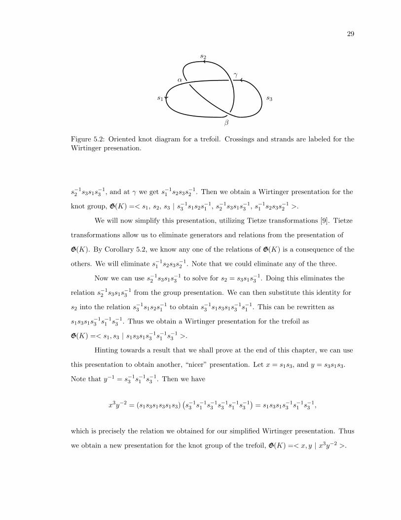
Example 5.3. Let us compute a Wirtinger presentation for the trefoil of Figure 2.3.
Orient the knot diagram and label its strands and crossings as in Figure 5.2.
At each crossing, we perform the procedure outlined above for computing relations
of the knot group. At crossing α, we obtain the relation s−13 s1s2s−11 . At β we get
29
s1 s3
s2
α
β
γ
Figure 5.2: Oriented knot diagram for a trefoil. Crossings and strands are labeled for theWirtinger presenation.
s−12 s3s1s−13 , and at γ we get s−11 s2s3s
−12 . Then we obtain a Wirtinger presentation for the
knot group, G(K) =< s1, s2, s3 | s−13 s1s2s−11 , s−12 s3s1s
−13 , s−11 s2s3s
−12 >.
We will now simplify this presentation, utilizing Tietze transformations [9]. Tietze
transformations allow us to eliminate generators and relations from the presentation of
G(K). By Corollary 5.2, we know any one of the relations of G(K) is a consequence of the
others. We will eliminate s−11 s2s3s−12 . Note that we could eliminate any of the three.
Now we can use s−12 s3s1s−13 to solve for s2 = s3s1s
−13 . Doing this eliminates the
relation s−12 s3s1s−13 from the group presentation. We can then substitute this identity for
s2 into the relation s−13 s1s2s−11 to obtain s−13 s1s3s1s
−13 s−11 . This can be rewritten as
s1s3s1s−13 s−11 s−13 . Thus we obtain a Wirtinger presentation for the trefoil as
G(K) =< s1, s3 | s1s3s1s−13 s−11 s−13 >.
Hinting towards a result that we shall prove at the end of this chapter, we can use
this presentation to obtain another, “nicer” presentation. Let x = s1s3, and y = s3s1s3.
Note that y−1 = s−13 s−11 s−13 . Then we have
x3y−2 = (s1s3s1s3s1s3)(s−13 s−11 s−13 s−13 s−11 s−13
)= s1s3s1s
−13 s−11 s−13 ,
which is precisely the relation we obtained for our simplified Wirtinger presentation. Thus
we obtain a new presentation for the knot group of the trefoil, G(K) =< x, y | x3y−2 >.

30
We will now adapt the Wirtinger presentation for butterfly diagrams. Let K be a
knot and BK a butterfly diagram for K. We assume that BK contains no E-vertices, since
we can always use inverse trunk-reducing moves to obtain an equivalent butterfly diagrams
with E-vertices replaced by simple butterflies. Let t1, t2, . . ., tm be the trunks of BK . The
trunks of BK will correspond to generators of G(K). Assign a consistent orientation to the
trunks of BK . That is, assign orientations to the trunks in such a way that if we apply the
butterfly-link algorithm on BK , the resulting knot diagram is oriented. To obtain relations
for G(K), we will perform the following procedure for each pair of tj-equivalent A-vertices.
Let ai and ak be A-vertices of BK which are tj-equivalent. Suppose that ai is an
endpoint of the trunk ti and ak is an endpoint of the trunk tk. Without loss of generality,
suppose ti is oriented so that it is leaving the butterfly containing tj . Then tk must be
oriented so that it is entering the butterfly containing tj . We then obtain a relation
ri = t−1i t=εij tktεij , where εi is determined via Figure 5.3.
ti
tk
tj
εi = 1
ti
tk
tj
εi = −1
Figure 5.3: Obtaining relations for the Wirtinger presentation from a butterfly diagram.

31
Since the identification of A-vertices across a trunk corresponds to a crossing in a
knot diagram, and each trunk corresponds to a strand, it is easy to see that this process is
equivalent to the standard method for obtaining a Wirtinger presentation. We would like
to simplify the process by eliminating unnecessary generators from the presentation. It
turns out we can eliminate the generators corresponding to simple butterflies (and
E-vertices).
Theorem 5.4. Let K be a knot and BK an oriented butterfly diagram of K with no
E-vertices. Let t1, . . ., tm be the trunks of BK which are not contained in simple
butterflies. Then the knot group of K admits the presentation
G(K) =< t1, . . . , tm|R1, . . . , Rm >,
where Ri =(tit
εj1j1. . . t
εjnjn
)t−1k
(t−εjnjn
. . . t−εj1j1
), as in Figure 5.4, and with εjl determined
as in Figure 5.3 for l = 1, . . ., n.
ti
tj1
ej1
tj2
ej2
tjn
ejn
tjn+1
tk
Figure 5.4: Obtaining a relation for a presentation of G(K) from the equivalence class of aiunder '.
Proof. Let e1, . . ., e` be the trunks of BK which are contained in simple butterflies.
By performing trunk-reducing moves to each el we obtain a new butterfly diagram B′K
which is equivalent to BK and which contains no simple butterflies. Let e′1, . . ., e′` be the
E-vertices of B′K , with e′l obtained by performing a trunk-reducing move on the simple
butterfly of BK containing el.
32
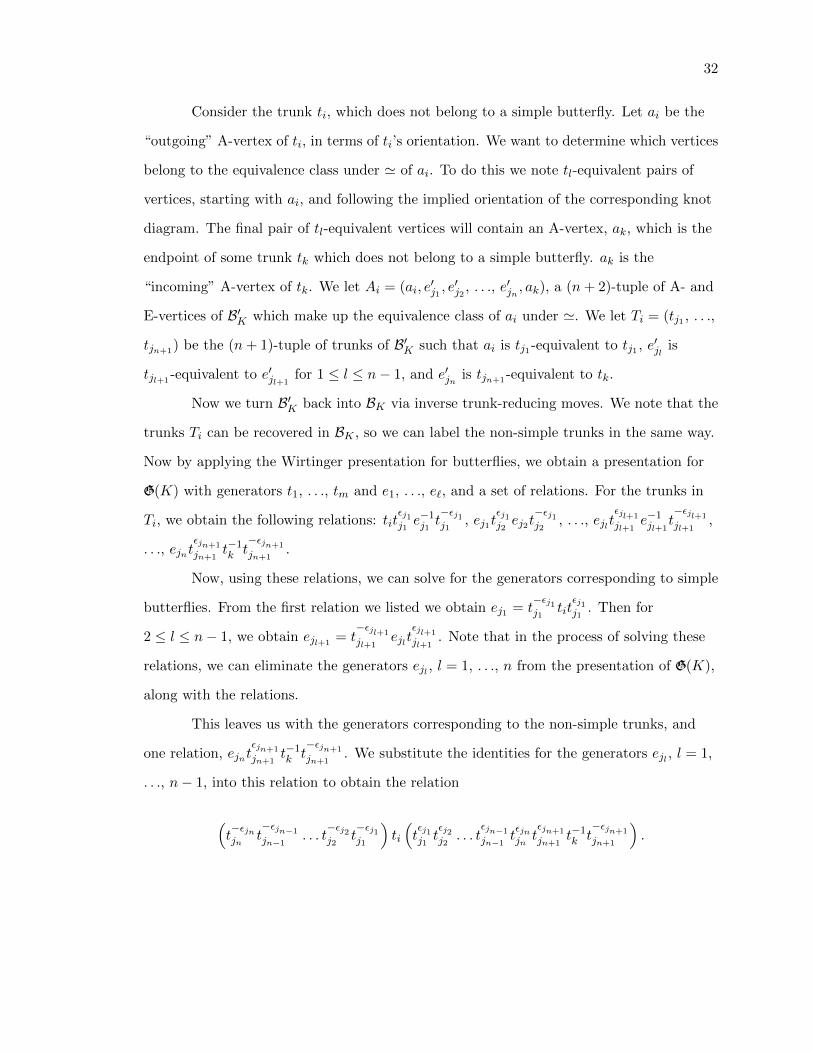
Consider the trunk ti, which does not belong to a simple butterfly. Let ai be the
“outgoing” A-vertex of ti, in terms of ti’s orientation. We want to determine which vertices
belong to the equivalence class under ' of ai. To do this we note tl-equivalent pairs of
vertices, starting with ai, and following the implied orientation of the corresponding knot
diagram. The final pair of tl-equivalent vertices will contain an A-vertex, ak, which is the
endpoint of some trunk tk which does not belong to a simple butterfly. ak is the
“incoming” A-vertex of tk. We let Ai = (ai, e′j1, e′j2 , . . ., e′jn , ak), a (n+ 2)-tuple of A- and
E-vertices of B′K which make up the equivalence class of ai under '. We let Ti = (tj1 , . . .,
tjn+1) be the (n+ 1)-tuple of trunks of B′K such that ai is tj1-equivalent to tj1 , e′jl is
tjl+1-equivalent to e′jl+1
for 1 ≤ l ≤ n− 1, and e′jn is tjn+1-equivalent to tk.
Now we turn B′K back into BK via inverse trunk-reducing moves. We note that the
trunks Ti can be recovered in BK , so we can label the non-simple trunks in the same way.
Now by applying the Wirtinger presentation for butterflies, we obtain a presentation for
G(K) with generators t1, . . ., tm and e1, . . ., e`, and a set of relations. For the trunks in
Ti, we obtain the following relations: titεj1j1e−1j1 t
−εj1j1
, ej1tεj1j2ej2t
−εj1j2
, . . ., ejltεjl+1
jl+1e−1jl+1
t−εjl+1
jl+1,
. . ., ejntεjn+1
jn+1t−1k t
−εjn+1
jn+1.
Now, using these relations, we can solve for the generators corresponding to simple
butterflies. From the first relation we listed we obtain ej1 = t−εj1j1
titεj1j1
. Then for
2 ≤ l ≤ n− 1, we obtain ejl+1= t−εjl+1
jl+1ejlt
εjl+1
jl+1. Note that in the process of solving these
relations, we can eliminate the generators ejl , l = 1, . . ., n from the presentation of G(K),
along with the relations.
This leaves us with the generators corresponding to the non-simple trunks, and
one relation, ejntεjn+1
jn+1t−1k t
−εjn+1
jn+1. We substitute the identities for the generators ejl , l = 1,
. . ., n− 1, into this relation to obtain the relation
(t−εjnjn
t−εjn−1
jn−1. . . t
−εj2j2
t−εj1j1
)ti
(tεj1j1tεj2j2. . . t
εjn−1
jn−1tεjnjntεjn+1
jn+1t−1k t
−εjn+1
jn+1
).

33
We can rewrite this relation as
(tit
εj1j1tεj2j2. . . t
εjn−1
jn−1tεjnjntεjn+1
jn+1
)t−1k
(t−εjn+1
jn+1t−εjnjn
t−εjn−1
jn−1. . . t
−εj2j2
t−εj1j1
),
as desired. �
Example 5.5. As an application of Theorem 5.4, let us compute a presentation for the
knot group of the (3,2)-torus knot. We orient and label the trunks of the butterfly
diagram in Figure 5.5. The generators of the knot group will correspond to the trunks t1
and t2. We also label the E-vertices as e1 and e2, and we label the A-vertices as a1, a′1, a2,
and a′2. b0 and ∞ are B-vertices as in the construction of the canonical butterfly diagram
as described in Chapter 4.
b0e1 e2 a′1
a′2 a2a1
t1
t2
∞∞
Figure 5.5: Oriented (3,2)-torus knot butterfly diagram, labeled for the Wirtinger presen-tation.
To determine the relations R1 and R2, we must first determine the equivalence
classes, under the relation ' on S2 = B3, of the A- and E-vertices of the diagram. By
following the orientation of t1, we obtain A1 = (a′1, e1, a2) and T1 = (t2, t1), as in the proof
of Theorem 5.4. That is, a′1 is t2-equivalent to e1, and e1 is t1-equivalent to a2. Similarly,
we have A2 = (a′2, e2, a1) and T2 = (t1, t2).
Thus we obtain the relations R1 = s1s2s1s−12 s−11 s−12 and R2 = s2s1s2s
−11 s−12 s−11 .
Thus we obtain a Wirtinger presentation for G(K) as G(K) =< s1, s2 | R1, R2 >. Note
That R2 = R−11 . Thus R2 is redundant, so we can remove it from our presentation of
34
G(K). Then we can express G(K) with only one relation, R1. We can, however, simplify
the presentation even further. Let x = s1s2 and y = s2s1s2. Then x3y−2 = R1. Thus we
obtain G(K) =< x, y | x3y−2 >, just as we did in Example 5.3.
Recall that by Theorem 4.1, we know that the (3,2)-torus knot and the (2,3)-torus
knot are equivalent. So we should not be surprised that we obtained the same knot group
presentation for both butterfly diagrams. What is interesting to note is that the
(2,3)-torus knot admits a knot group presentation whose sole relation is x2y−3. We
generalize this result in the following theorem.
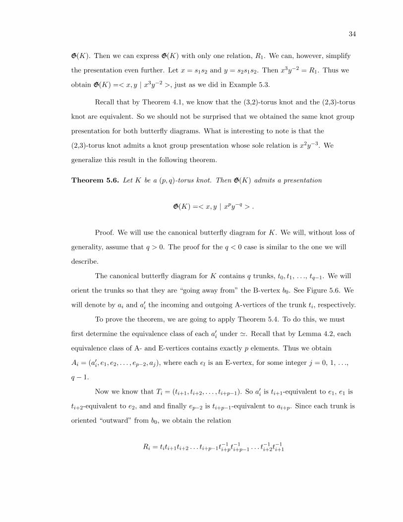
Theorem 5.6. Let K be a (p, q)-torus knot. Then G(K) admits a presentation
G(K) =< x, y | xpy−q > .
Proof. We will use the canonical butterfly diagram for K. We will, without loss of
generality, assume that q > 0. The proof for the q < 0 case is similar to the one we will
describe.
The canonical butterfly diagram for K contains q trunks, t0, t1, . . ., tq−1. We will
orient the trunks so that they are “going away from” the B-vertex b0. See Figure 5.6. We
will denote by ai and a′i the incoming and outgoing A-vertices of the trunk ti, respectively.
To prove the theorem, we are going to apply Theorem 5.4. To do this, we must
first determine the equivalence class of each a′i under '. Recall that by Lemma 4.2, each
equivalence class of A- and E-vertices contains exactly p elements. Thus we obtain
Ai = (a′i, e1, e2, . . . , ep−2, aj), where each el is an E-vertex, for some integer j = 0, 1, . . .,
q − 1.
Now we know that Ti = (ti+1, ti+2, . . . , ti+p−1). So a′i is ti+1-equivalent to e1, e1 is
ti+2-equivalent to e2, and and finally ep−2 is ti+p−1-equivalent to ai+p. Since each trunk is
oriented “outward” from b0, we obtain the relation
Ri = titi+1ti+2 . . . ti+p−1t−1i+pt
−1i+p−1 . . . t
−1i+2t
−1i+1

35
∞
∞
∞
∞
∞
a′0
a0
t0
t1
t2
t3
Figure 5.6: Oriented (p, q)-torus link butterfly diagram.
for each i = 0, . . . , q − 1, with the indices of the trunks taken modulo q.
To simplify our notation, we will let Xi = titi+1ti+2 . . . ti+p−1, for i = 0, . . . , q − 1,
and the indices of trunks taken modulo q. Then we can rewrite our relations as
Ri = XiX−1i+1. We thus obtain a presentation of the knot group of K as
G(K) =< t0, . . . , tq−1 | R0, . . . , Rq−1 >. Our next goal is to simplify this presentation so
as to match the presentation in the statement of the theorem.
Consider X0X`1X`2 . . . X`q−1 = (t0t1 . . . tq−1)p, where `j ≡ jp (mod q). Also note
that since Ri = XiX−1i+1, we obtain Xi = Xi+1. From this it follows that
X1 = X2 = . . . = Xq−1. Note that Rq−1 = Xq−1X−10 . Then in G(K), Xq−1 = X0.
However, this has already been determined from the relations R0, R1, . . ., Rq−2. Thus
Rq−1 is redundant, so we can eliminate it from our presentation of G(K).
36
Now note that, in particular, X1 = X`j for any j. Thus
(t0t1 . . . tq−1)p(X−11 )q = (X0X`1 . . . X`q−1)(X−1`q−1
. . . X−1`1 X−11 ) = X0X
−11 .
But X0X−11 is a relation of the group, and is thus trivial. So it follows that
(t0 . . . tq−1)p(X−11 )q = 1.
Let x = t0 . . . tq−1 and y = X1. Then we obtain xpy−q = 1. Thus we can rewrite
the knot group of K as G(K) =< x, y | xpy−q >. �
37
CHAPTER 6
BUTTERFLY MOVES AND REIDEMEISTER’S THEOREM
In Chapter 2, we saw that a given knot may have many knot diagrams. Recall
that by Reidemeister’s Theorem, any two diagrams for a given knot can be related by a
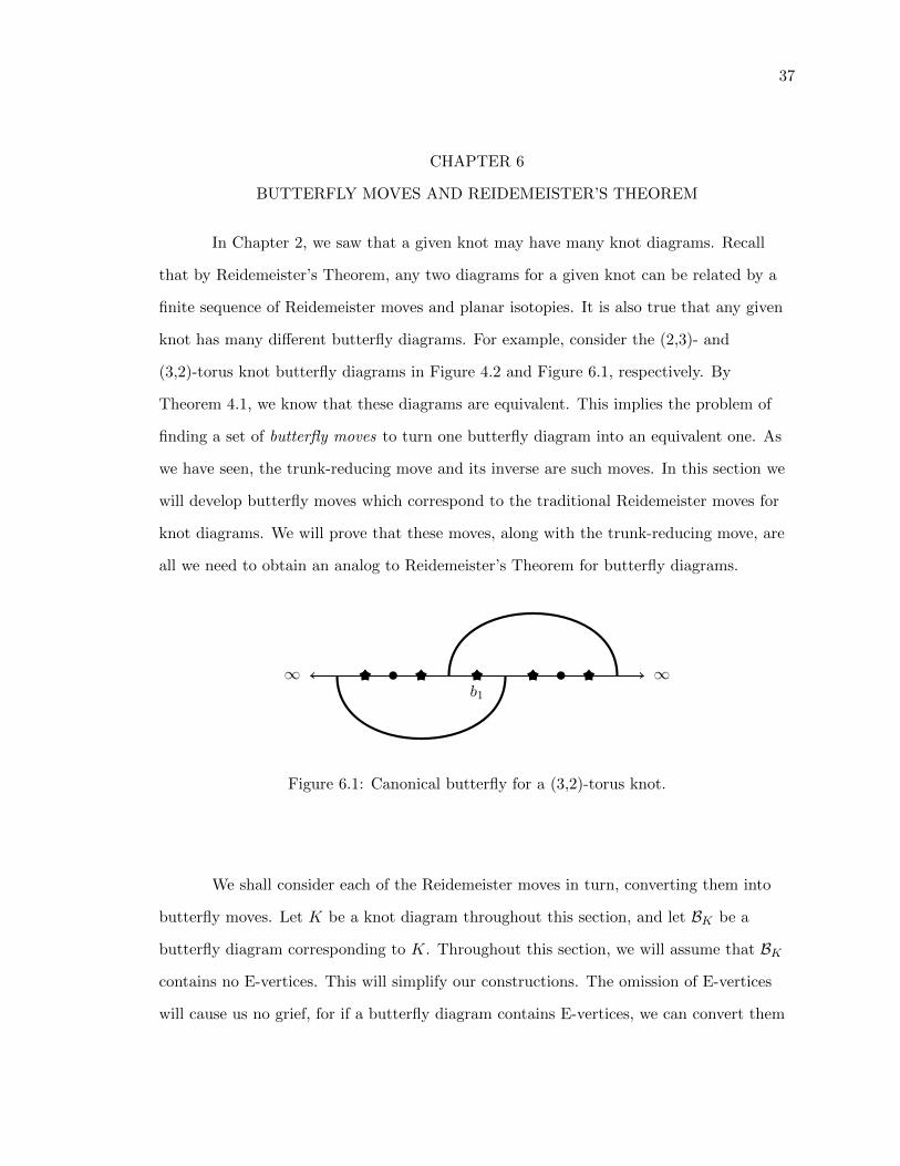
finite sequence of Reidemeister moves and planar isotopies. It is also true that any given
knot has many different butterfly diagrams. For example, consider the (2,3)- and
(3,2)-torus knot butterfly diagrams in Figure 4.2 and Figure 6.1, respectively. By
Theorem 4.1, we know that these diagrams are equivalent. This implies the problem of
finding a set of butterfly moves to turn one butterfly diagram into an equivalent one. As
we have seen, the trunk-reducing move and its inverse are such moves. In this section we
will develop butterfly moves which correspond to the traditional Reidemeister moves for
knot diagrams. We will prove that these moves, along with the trunk-reducing move, are
all we need to obtain an analog to Reidemeister’s Theorem for butterfly diagrams.
b1∞∞
Figure 6.1: Canonical butterfly for a (3,2)-torus knot.
We shall consider each of the Reidemeister moves in turn, converting them into
butterfly moves. Let K be a knot diagram throughout this section, and let BK be a
butterfly diagram corresponding to K. Throughout this section, we will assume that BK
contains no E-vertices. This will simplify our constructions. The omission of E-vertices
will cause us no grief, for if a butterfly diagram contains E-vertices, we can convert them
38
to simple butterflies via inverse trunk-reducing moves, perform our butterfly moves, and
then convert the simple butterflies back into E-vertices.
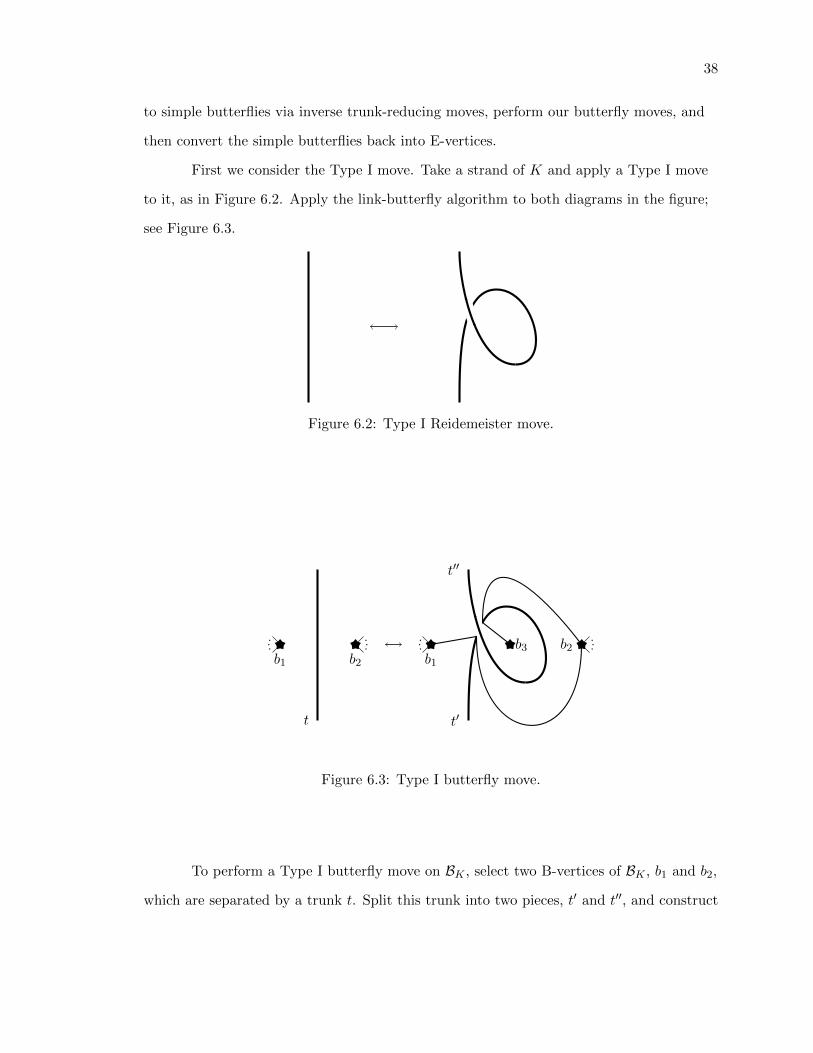
First we consider the Type I move. Take a strand of K and apply a Type I move
to it, as in Figure 6.2. Apply the link-butterfly algorithm to both diagrams in the figure;
see Figure 6.3.
Figure 6.2: Type I Reidemeister move.
t t′
t′′
b1 b2 b1b3 b2
Figure 6.3: Type I butterfly move.
To perform a Type I butterfly move on BK , select two B-vertices of BK , b1 and b2,
which are separated by a trunk t. Split this trunk into two pieces, t′ and t′′, and construct
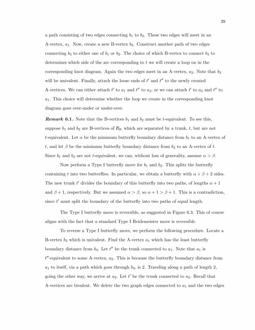
39
a path consisting of two edges connecting b1 to b2. These two edges will meet in an
A-vertex, a1. Now, create a new B-vertex b3. Construct another path of two edges
connecting b3 to either one of b1 or b2. The choice of which B-vertex to connect b3 to
determines which side of the arc corresponding to t we will create a loop on in the
corresponding knot diagram. Again the two edges meet in an A-vertex, a2. Note that b3
will be univalent. Finally, attach the loose ends of t′ and t′′ to the newly created
A-vertices. We can either attach t′ to a1 and t′′ to a2, or we can attach t′ to a2 and t′′ to
a1. This choice will determine whether the loop we create in the corresponding knot
diagram goes over-under or under-over.
Remark 6.1. Note that the B-vertices b1 and b2 must be t-equivalent. To see this,
suppose b1 and b2 are B-vertices of BK which are separated by a trunk, t, but are not
t-equivalent. Let α be the minimum butterfly boundary distance from b1 to an A-vertex of
t, and let β be the minimum butterfly boundary distance from b2 to an A-vertex of t.
Since b1 and b2 are not t-equivalent, we can, without loss of generality, assume α > β.
Now perform a Type I butterfly move for b1 and b2. This splits the butterfly
containing t into two butterflies. In particular, we obtain a butterfly with α+ β + 2 sides.
The new trunk t′ divides the boundary of this butterfly into two paths, of lengths α+ 1
and β + 1, respectively. But we assumed α > β, so α+ 1 > β + 1. This is a contradiction,
since t′ must split the boundary of the butterfly into two paths of equal length.
The Type I butterfly move is reversible, as suggested in Figure 6.3. This of course
aligns with the fact that a standard Type I Reidemeister move is reversible.
To reverse a Type I butterfly move, we perform the following procedure. Locate a
B-vertex b3 which is univalent. Find the A-vertex a1 which has the least butterfly
boundary distance from b3. Let t′′ be the trunk connected to a1. Note that a1 is
t′′-equivalent to some A-vertex, a2. This is because the butterfly boundary distance from
a1 to itself, via a path which goes through b3, is 2. Traveling along a path of length 2,
going the other way, we arrive at a2. Let t′ be the trunk connected to a2. Recall that
A-vertices are bivalent. We delete the two graph edges connected to a1 and the two edges
40
connected to a2, along with the vertex b3. We fuse the loose ends of t′ and t′′, to make a
new trunk t.
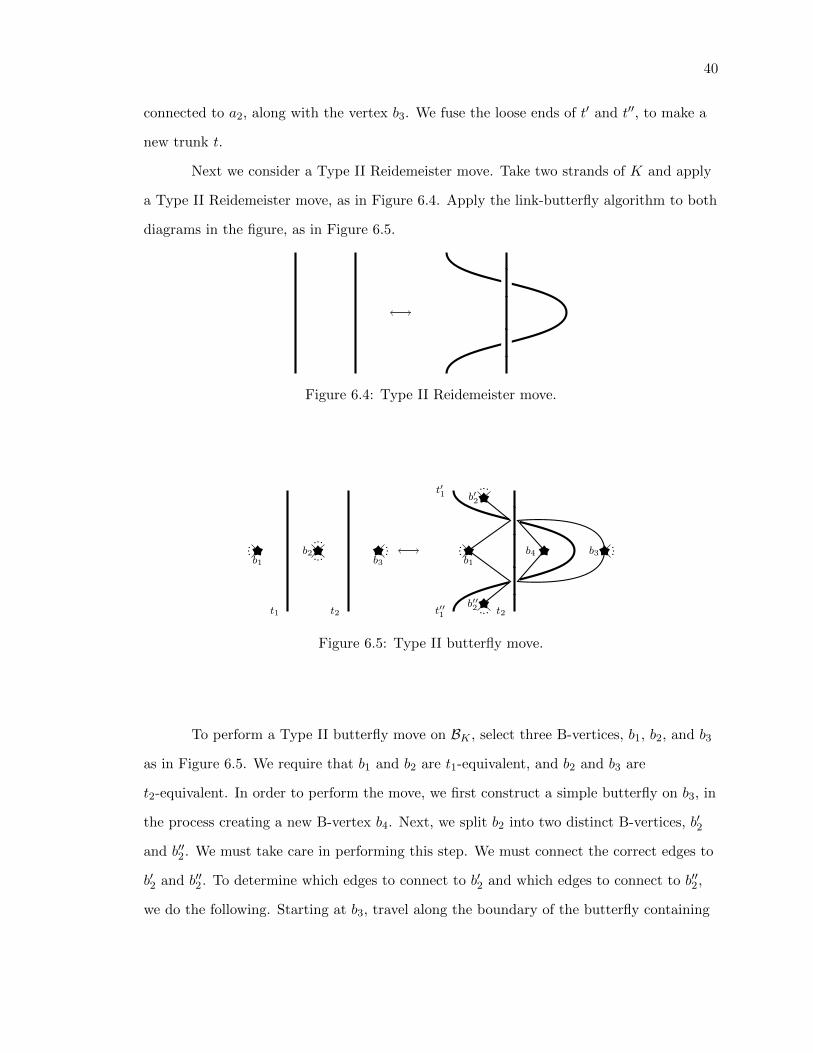
Next we consider a Type II Reidemeister move. Take two strands of K and apply
a Type II Reidemeister move, as in Figure 6.4. Apply the link-butterfly algorithm to both
diagrams in the figure, as in Figure 6.5.
Figure 6.4: Type II Reidemeister move.
t1 t2 t2t′′1
t′1
b1b2
b3 b1
b′2
b′′2
b3b4
Figure 6.5: Type II butterfly move.
To perform a Type II butterfly move on BK , select three B-vertices, b1, b2, and b3
as in Figure 6.5. We require that b1 and b2 are t1-equivalent, and b2 and b3 are
t2-equivalent. In order to perform the move, we first construct a simple butterfly on b3, in
the process creating a new B-vertex b4. Next, we split b2 into two distinct B-vertices, b′2
and b′′2. We must take care in performing this step. We must connect the correct edges to
b′2 and b′′2. To determine which edges to connect to b′2 and which edges to connect to b′′2,
we do the following. Starting at b3, travel along the boundary of the butterfly containing
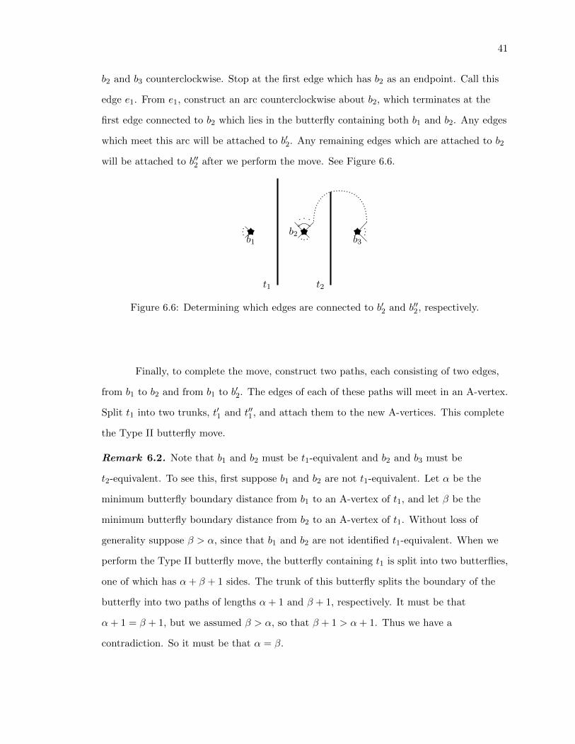
41
b2 and b3 counterclockwise. Stop at the first edge which has b2 as an endpoint. Call this
edge e1. From e1, construct an arc counterclockwise about b2, which terminates at the
first edge connected to b2 which lies in the butterfly containing both b1 and b2. Any edges
which meet this arc will be attached to b′2. Any remaining edges which are attached to b2
will be attached to b′′2 after we perform the move. See Figure 6.6.
t1 t2
b1b2
b3
Figure 6.6: Determining which edges are connected to b′2 and b′′2, respectively.
Finally, to complete the move, construct two paths, each consisting of two edges,
from b1 to b2 and from b1 to b′2. The edges of each of these paths will meet in an A-vertex.
Split t1 into two trunks, t′1 and t′′1, and attach them to the new A-vertices. This complete
the Type II butterfly move.
Remark 6.2. Note that b1 and b2 must be t1-equivalent and b2 and b3 must be
t2-equivalent. To see this, first suppose b1 and b2 are not t1-equivalent. Let α be the
minimum butterfly boundary distance from b1 to an A-vertex of t1, and let β be the
minimum butterfly boundary distance from b2 to an A-vertex of t1. Without loss of
generality suppose β > α, since that b1 and b2 are not identified t1-equivalent. When we
perform the Type II butterfly move, the butterfly containing t1 is split into two butterflies,
one of which has α+ β + 1 sides. The trunk of this butterfly splits the boundary of the
butterfly into two paths of lengths α+ 1 and β + 1, respectively. It must be that
α+ 1 = β + 1, but we assumed β > α, so that β + 1 > α+ 1. Thus we have a
contradiction. So it must be that α = β.

42
Next we want to show that b2 and b3 must be t2-equivalent. Let β be the
minimum butterfly boundary distance from b2 to an A-vertex of t2, and let γ be the
minimum butterfly boundary distance from b3 to an A-vertex of t2. Without loss of
generality, suppose γ > β, so that b2 and b3 are not t2-equivalent. Perform a Type II
butterfly move, which creates a simple butterfly on b3. We label the other B-vertex of this
simple butterfly as b4. In the resulting butterfly diagram, we label A-vertices as follows.
The A-vertex between b1 and b′2 is labeled as a1, the A-vertex between b′2 and b3 is labeled
as a2, and the A-vertex between b3 and b4 is labeled as a3. For the butterfly move to
correspond to a Type II Reidemeister move, we expect a1 and a3 to be t2-equivalent.
However, the butterfly boundary distance from a1 to a2 is β + 1, and the butterfly
boundary distance from a2 to a3 is γ + 1. Since we assumed β < γ, this implies that a1
and a3 are not t2-equivalent. Thus the butterfly move will not correspond to a Type II
Reidemeister move. We conclude that b2 and b3 must be t2-equivalent.
The Type II butterfly move is reversible, just as the Type I move is. To perform
an inverse Type II butterfly move, we do the following. Select a simple butterfly of BK ,
with B-vertices b3 and b4, as in Figure 6.5. Locate B-vertices which are separated from b3
and b4 by a trunk, t2, label them b′2, b′′2, and b1, as in Figure 6.5. We require that b3 is
t2-equivalent to both b′2 and b′′2, and that b4 is t2-equivalent to b1. Two trunks, t′1 and t′′1,
have A-vertices between b′2 and b1, and b′′2 and b1, respectively. To perform the inverse
Type II move, delete the simple butterfly containing b3 and b4, leaving only b3 in its place.
Next delete the edges connecting b1 to b′2 and b1 to b′′2, and fuse the loose ends of t′1 and t′′1
to form a new trunk, t1. Finally, combine b′2 and b′′2 into a single B-vertex, b2.
Finally we consider Type III Reidemeister moves. Suppose K has an arrangement
of strands as in Figure 6.7. Apply the link-butterfly algorithm to both diagrams in the
figure, as in Figure 6.8.
To perform a Type III butterfly move on BK , we first locate a configuration as in
Figure 6.8. The B-vertices b1 and b3 must be t3-equivalent, b2 and b6 must be
t1-equivalent, and b1 and b4 must be t1-equivalent. We simply replace the edges between

43
Figure 6.7: Type III Reidemeister move.
t1
t2
t3 t1
t2
t3
b1 b6
b3
b4
b2
b5
b1 b6
b2
b5
b3
b4
Figure 6.8: Type III butterfly move.
b1, b2, and b3, and b4, b5, and b6, as shown in the figure. Note that the simple butterfly is
moved entirely from one side of t1 to the other.
Example 6.3. We now present an example which will apply each of the butterfly moves
just described. We will transform a canonical butterfly diagram for the twist knot T2 into
an equivalent butterfly diagram via a sequence of butterfly moves. The sequence of
butterfly moves is depicted in Figure 6.10. To help the reader see how the moves are
applied, we provide the analogous sequence of Reidemeister moves, applied to a knot
diagram of T2, in Figure 6.9. The reader is encouraged to compare the diagrams in each
figure to see how they relate. The reader may also find it useful to perform the
butterfly-link algorithm to the butterfly diagrams in Figure 6.10, and to compare their
results with the knot diagrams in Figure 6.9.
Furthermore, we have labeled B-vertices and trunks of the butterfly diagrams

44
(a) The twist knot T2 (b) Applying a Type II.
(c) Applying a Type III. (d) Applying a Type I.
Figure 6.9: Performing a sequence of Reidemeister moves on T2.
similarly to our discussions of the butterfly moves earlier in this chapter. So in Figure
6.10a, we have labeled B-vertices b1, b2, and b3, which the relevant B-vertices for
performing the desired Type II move. In Figure 6.10b, the B-vertices b1, b2, b3 = b6, b4,
and b5 are the relevant B-vertices for performing the desired Type III move. We note that
b3 = b6. As a result, by performing the Type III move, we obtain a butterfly diagram
which contains a univalent B-vertex, which corresponds to b2.
Finally, in Figure 6.10c, the B-vertices b1, b2, and b3 are the relevant B-vertices for
performing an inverse Type I move. Figure 6.10d depicts the end result of the sequence of

45
b3
b2
b1
(a) Canonical butterfly for T2, prepped for aType II move.
b4
b5
b3 = b6
b2b1
(b) After applying a Type II move, andprepped for a Type III move.
b3b2
b1
(c) After applying a Type III move, andprepped for a Type I move. (d) After applying a Type I move.
Figure 6.10: Performing a sequence of butterfly moves on a butterfly diagram for T2, whichis analogous to the moves in Figure 6.9.
butterfly moves.
Recall that two butterfly diagrams are said to be equivalent if they correspond to
the same link. Thus far, we have defined four types of butterfly moves: three moves which
are analogous to the Reidemeister moves for knot diagrams, and trunk-reducing moves.
These moves transform a given butterfly diagram into an equivalent one. It is natural to
ask if there are any other moves that we need to investigate in order to define equivalence
for butterfly diagrams. It turns out that we do not.
Theorem 6.4. Let B1 and B2 be butterfly diagrams for a link L. Then B1 is equivalent to

46
B2 if and only if there is a finite sequence of butterfly moves which transforms B1 into B2.
Proof. First suppose there exists a finite sequence of butterfly moves which
transforms B1 into B2. We know that trunk-reducing moves and their inverses do not alter
the link diagram corresponding to a given butterfly diagram. Furthermore, Type I, II, and
III butterfly moves are equivalent to Reidemeister moves on the corresponding link
diagrams. Thus if two butterfly diagrams are related by a single Type I, II, or III butterfly
move, then they must be equivalent. So it follows that B1 and B2 are equivalent.
Conversely, suppose B1 and B2 are equivalent. Let D1 and D2 be the link diagrams
corresponding to B1 and B2, respectively. We perform inverse trunk-reducing moves to B1
to obtain an equivalent butterfly diagram B′1 which does not contain any E-vertices. Not
only are B1 and B′1 equivalent, but they have the exact same corresponding link diagram,
D1. Similarly, we can obtain a butterfly diagram B′2 which is equivalent to B2 and to
which D2 corresponds. Now since B1 and B2 where assumed to be equivalent, it must be
that B′1 and B′2 are equivalent. In addition, it must be that D1 and D2 are equivalent as
link diagrams. Thus by Theorem 2.6, there exists a finite sequence of Reidemeister moves
and planar isotopies which transform D1 into D2. Now, planar isotopies on a link diagram
do not alter corresponding butterfly diagrams, so we omit them from consideration. Each
of the Reidemeister moves in the sequence taking D1 to D2 has an equivalent butterfly
move. Thus we can apply these butterfly moves in the proper order, beginning with B′1,
and obtaining B′2. Finally, perform inverse trunk-reducing moves to B′2 to obtain B2. Thus
we have constructed a sequence of butterfly moves transforming B1 into B2. �
Theorem 6.4 defines equivalence of butterfly diagrams in a way that is analogous
to Theorem 2.6 for link diagrams. We take caution by noting that our constructions of
butterfly moves are specific to our restricted definition of butterfly diagram. Thus while
for our definition of butterfly diagram the moves we have described are enough to define
equivalence, this may not be the case for the more general definition of butterfly diagram
initially proposed by HMTT.

47
CHAPTER 7
CLASSIFICATION OF 1-BUTTERFLIES
The next few chapters will focus on the classification of links by their butterfly
number. Recall that Theorem 3.9 states that the butterfly number of a link is equivalent
to its bridge number. Thus classifying links by their butterfly number is equivalent to
classifying them by their bridge number. The latter classification is well known for 1- and
2-bridge links. The classification of 3-bridge links is still an open problem. It is our goal to
recreate the classifications of 1- and 2-bridge links via their butterfly diagrams. Thus we
will classify 1- and 2-butterflies.
We begin by studying 1-butterflies. It is well known that any 1-bridge link is the
unknot. The same holds for butterflies.
Theorem 7.1. Let L be a link. Then L is the unknot if and only if m(L) = 1.
Before proving Theorem 7.1, we need to discuss some properties of 1-butterfly
diagrams in general. Let B = (R, T ) be a 1-butterfly. By definition, R is embedded on
S2 = ∂B3 so that S2 \R is a single 2-cell (in other words, S2 \R is homeomorphic to a
disk). If R contained any cycles, then R would necessarily divide S2 into more than one
2-cell. Thus for B to be a 1-butterfly, it must be that R is a finite tree.
A vertex of a tree which has degree equal to one is called a leaf. Since we will only
consider finite trees, R will always have a leaf. Furthermore, since we require A- and
E-vertices to be bivalent in R, it follows that if a vertex of R is a leaf, then it is a B-vertex.
Since R divides S2 = ∂B3 into a single polygonal face, each edge of R has exactly
two edges of ∂P2n in its preimage under f : P2n → C ⊆ S2. Thus in measuring butterfly
boundary distance for B, each edge is double-counted. As a consequence of Theorem 3.12,
we have the following lemma.
Lemma 7.2. Let B be a 1-butterfly diagram. Suppose B’s only butterfly has N sides.
Then N is divisible by 4.

48
Proof. Let t be the unique trunk of B. Let D be the knot diagram corresponding
to B, via the butterfly-link algorithm. Let m be the number of underpasses of the arc of D
which corresponds to t. Then by Theorem 3.12, t belongs to a butterfly with 4(m+ 1)
sides. But B has exactly one butterfly, of which t is the trunk. This butterfly has N sides.
Thus N = 4(m+ 1), so 4 divides N . �
Since each edge of R is double-counted, Lemma 7.2 implies that R must have an
even number of edges when strictly considered as a graph, rather than the boundary of a
butterfly.
Our next lemma states that no 1-butterfly can have 0 or 4 sides. For a 1-butterfly
to be properly defined, it must have at least 8 sides.
Lemma 7.3. Let B = (R, T ) be a 1-butterfly diagram. Then B’s only butterfly has
4(n+ 1) sides, with n ≥ 1.
Proof. Suppose n = −1, so that B’s only butterfly has 0 sides. Then R has no
edges. Note, however, that R is connected. Thus R consists of a single vertex, which must
be a B-vertex. This is not a butterfly diagram, since there are no A-vertices, and hence no
trunks.
Next suppose n = 0. Then B’s only butterfly has 4 sides. This means that as a
graph, R is a tree with exactly two edges. Since R is a tree with two edges, it must have
two leaves, which are B-vertices, and one other vertex. This other vertex must be an
A-vertex. However, since it is the only A-vertex, there is no way to construct a trunk
which has distinct endpoints. See Figure 7.1. This violates our requirement that the
trunks of B must not have coincident endpoints. So if n = 0, B is not a butterfly diagram.
Thus it must be that n ≥ 1. �
Lemma 7.4. Let B = (R, T ) be a 1-butterfly diagram such that B’s only butterfly has
exactly 8 sides. Then R must be one of the graph in Figure 7.2, and B corresponds to the
unknot.
Proof. First we show by construction that R must match the graph of the

49
Figure 7.1: A 1-butterfly diagram cannot have four sides.
b1 b2 b3 b1 b2 b3
Figure 7.2: 8-sided 1-butterfly diagrams. The corresponding knot diagrams are mirrorimages of each other, and are the unknot.
butterfly in Figure 7.2. Note that since the butterfly has 8 sides, R must have exactly four
graph edges. Consider a leaf of R, which we know is a B-vertex. Label this B-vertex b1.
Since b1 is a leaf, it is univalent, and thus only has one edge, h1, connected to it. Since R
is bipartite, we know that the other vertex on h1 must be either an A- or E-vertex. Let x1
be this vertex. Thus b1 is connected to x1 by h1. Now A- and E-vertices are bivalent in R,
so x1 has another edge, h2, connected to it, and the other endpoint of h2 must be a
B-vertex. Label this vertex b2.
Now we have accounted for two of R’s four graph edges, so we must account for
two more. Note that it cannot be that b2 has degree three. If it did, then there would be
two edges attached to b2 distinct from h2. The endpoints of these edges would have to be

50
univalent in R. We know that any univalent vertex of R must be a B-vertex. Thus b2
would be connected to two B-vertices, contradicting the fact that R is bipartite.
Thus b2 must be bivalent in R. Let h3 be the edge connected to b2 which is
distinct from h2. We know that the other endpoint of h3 must be either an A- or E-vertex.
Let x2 be this vertex. Again, since A- and E-vertices of R must be bivalent, there is
another edge h4 attached to x2. The other endpoint of h4 must be a B-vertex, b3.
Thus we have constructed all four graph edges of R. Now, note that for us to be
able to properly place a trunk in B, R must contain exactly two A-vertices. Since x1 and
x2 are the only vertices of R which are not B-vertices, it follows that x1 and x2 must be
A-vertices.
Thus we obtain the graph of the butterfly diagrams in Figure 7.2. To see that both
of these diagrams correspond to the unknot, we simply apply the butterfly-link algorithm
to both of them and note that the resulting knot diagrams are clearly trivial. �
Now we are ready to prove Theorem 7.1. First we suppose m(L) = 1. Our goal is
to show that L is the unknot. Let BL be a 1-butterfly diagram for L, whose only butterfly
has 4(n+ 1) sides. We proceed by induction on n.
For our base case we consider n = 1. Note that by Lemma 7.3, we need not
consider the cases n = −1 or n = 0. Since n = 1, the butterfly in BL must have eight
sides, and so by Lemma 7.4, we know that L is the unknot.
Now suppose that for some positive integer n > 1 that any 1-butterfly with exactly
4(m+ 1) sides is trivial if m < n. We want to show that a 1-butterfly with exactly
4(n+ 1) sides is trivial. So suppose BL consists of a butterfly with 4(n+ 1) sides. Since
BL is a 1-butterfly diagram, its graph is a finite tree. Thus its graph has a leaf, which we
know is a B-vertex of degree equal to one. Let b1 be this B-vertex. Since b1 is univalent, it
is connected to exactly one graph edge, h1. Let x be the other vertex on h1. The vertex x
is either an A- or an E-vertex. So x is bivalent. Let h2 be the edge attached to x which is
distinct from h1, and let b2 be the B-vertex on h2’s other end. We now have two separate
cases to consider: x is an A-vertex and x is an E-vertex.
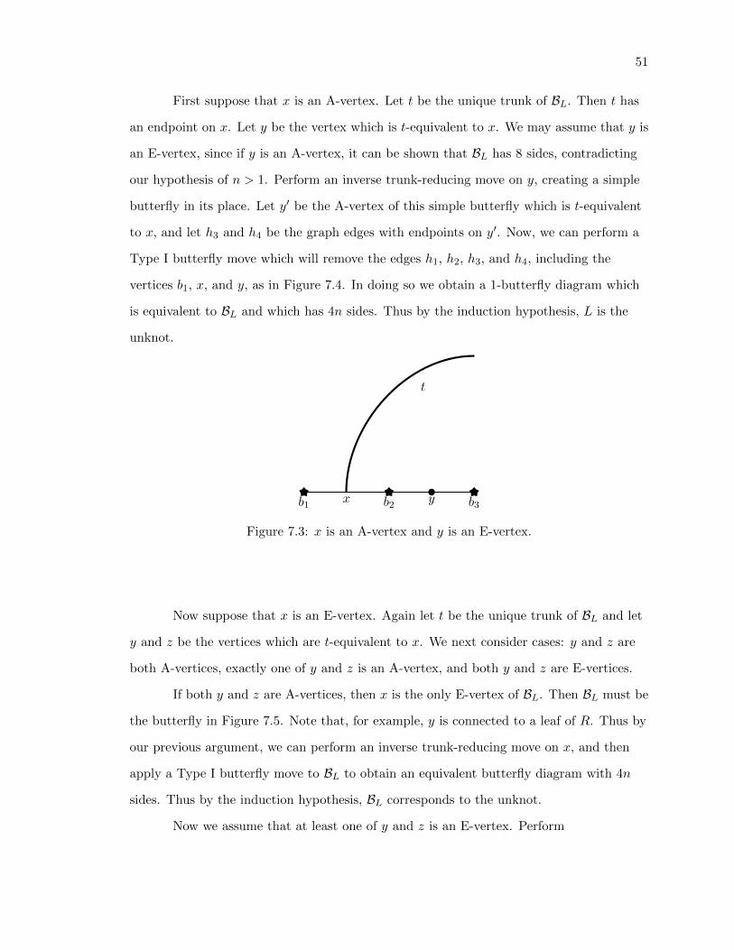
51
First suppose that x is an A-vertex. Let t be the unique trunk of BL. Then t has
an endpoint on x. Let y be the vertex which is t-equivalent to x. We may assume that y is
an E-vertex, since if y is an A-vertex, it can be shown that BL has 8 sides, contradicting
our hypothesis of n > 1. Perform an inverse trunk-reducing move on y, creating a simple
butterfly in its place. Let y′ be the A-vertex of this simple butterfly which is t-equivalent
to x, and let h3 and h4 be the graph edges with endpoints on y′. Now, we can perform a
Type I butterfly move which will remove the edges h1, h2, h3, and h4, including the
vertices b1, x, and y, as in Figure 7.4. In doing so we obtain a 1-butterfly diagram which
is equivalent to BL and which has 4n sides. Thus by the induction hypothesis, L is the
unknot.
x yb1 b2 b3
t
Figure 7.3: x is an A-vertex and y is an E-vertex.
Now suppose that x is an E-vertex. Again let t be the unique trunk of BL and let
y and z be the vertices which are t-equivalent to x. We next consider cases: y and z are
both A-vertices, exactly one of y and z is an A-vertex, and both y and z are E-vertices.
If both y and z are A-vertices, then x is the only E-vertex of BL. Then BL must be
the butterfly in Figure 7.5. Note that, for example, y is connected to a leaf of R. Thus by
our previous argument, we can perform an inverse trunk-reducing move on x, and then
apply a Type I butterfly move to BL to obtain an equivalent butterfly diagram with 4n
sides. Thus by the induction hypothesis, BL corresponds to the unknot.
Now we assume that at least one of y and z is an E-vertex. Perform
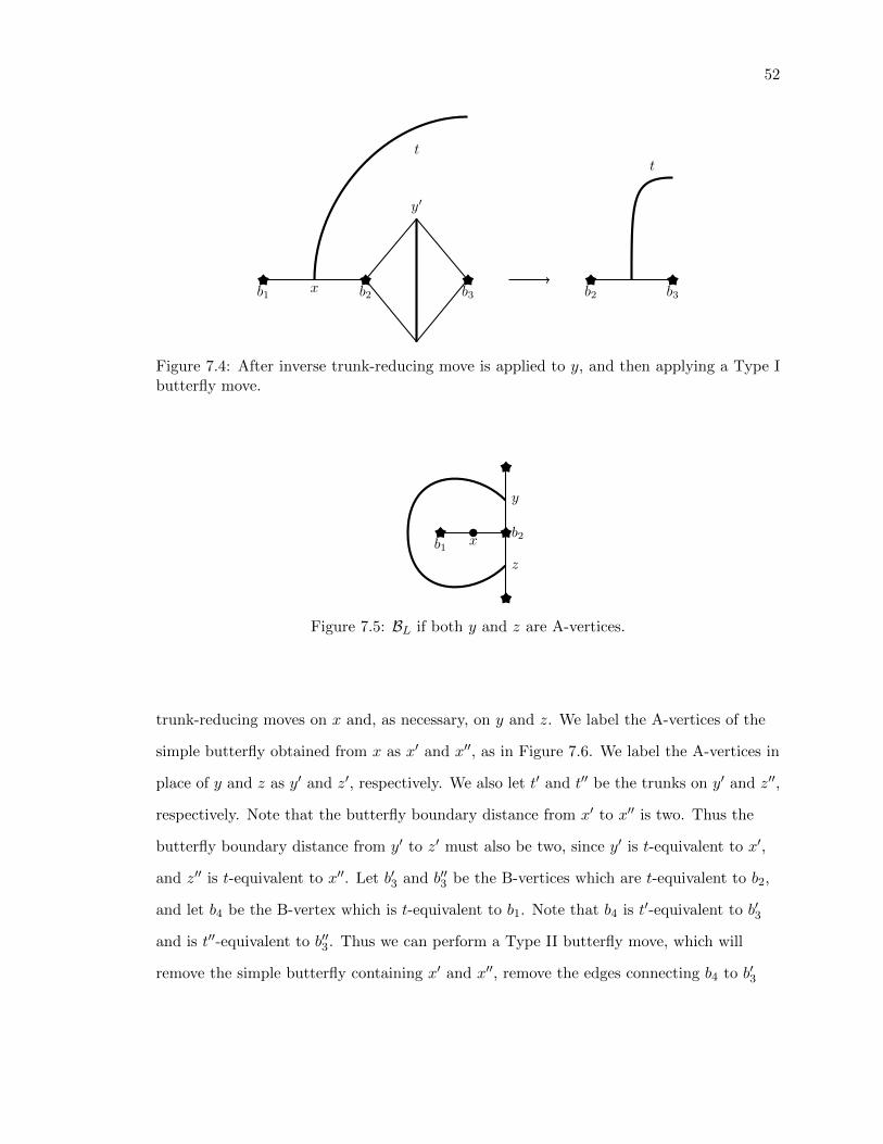
52
t
x
y′
b1 b2 b3 b2 b3
t
Figure 7.4: After inverse trunk-reducing move is applied to y, and then applying a Type Ibutterfly move.
xb1b2
y
z
Figure 7.5: BL if both y and z are A-vertices.
trunk-reducing moves on x and, as necessary, on y and z. We label the A-vertices of the
simple butterfly obtained from x as x′ and x′′, as in Figure 7.6. We label the A-vertices in
place of y and z as y′ and z′, respectively. We also let t′ and t′′ be the trunks on y′ and z′′,
respectively. Note that the butterfly boundary distance from x′ to x′′ is two. Thus the
butterfly boundary distance from y′ to z′ must also be two, since y′ is t-equivalent to x′,
and z′′ is t-equivalent to x′′. Let b′3 and b′′3 be the B-vertices which are t-equivalent to b2,
and let b4 be the B-vertex which is t-equivalent to b1. Note that b4 is t′-equivalent to b′3
and is t′′-equivalent to b′′3. Thus we can perform a Type II butterfly move, which will
remove the simple butterfly containing x′ and x′′, remove the edges connecting b4 to b′3

53
and b4 to b′′3, combine b′3 and b′′3 into a single B-vertex, and will combine the trunks t′ and
t′′ into a single trunk s. See Figure 7.6.
tx′′
x′y′
z′′
b1 b2
b′3
b4
b′′3
t′
t′′
b2 b3 b4
t s
Figure 7.6: After applying inverse trunk-reducing moves to all E-vertices of BL, and theresult of a Type II butterfly move.
Next, we claim that by performing a Type II butterfly move, we create at most
one simple butterfly. To show this, we consider two cases: exactly one of y1 and y2 is an
E-vertex, and both y1 and y2 are E-vertices. First, we suppose, without loss of generality,
that y1 is an E-vertex, and that y2 is an A-vertex. An argument similar to the one we
present holds if the roles of y1 and y2 are reversed.
Since y is an E-vertex, we perform an inverse trunk-reducing move to create a
simple butterfly in its place. Notice that since z is an A-vertex, t′′ = t. When we perform
a Type II move to remove the simple butterfly obtained from x, we also remove two edges
from the simple butterfly on y′. The result is as in Figure 7.7. Notice that the trunk s,
obtained from combining t and t′, actually coincides with t. As a result, no new butterflies
are created at all, so the result of performing a Type II move is still a 1-butterfly diagram.
Next suppose that both y1 and y2 are E-vertices. Then we perform inverse trunk-reducing
moves on both y1 and y2, creating simple butterflies in their places. In this case, when we
perform a Type II move to remove the simple butterfly on x, we create a simple butterfly.
Note that the trunk of this simple butterfly is s, which we obtain by combining the trunks
t′ and t′′. See Figure 7.8. Notice that we do not create any other new butterflies. Also
note that the butterfly diagram we obtain has 8 fewer sides. Thus performing a Type II
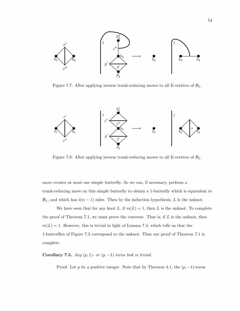
54
tx′
x′′y′
z′′
b1 b2
b′3
b4
b′′3
t′
t
b2 b4b3
Figure 7.7: After applying inverse trunk-reducing moves to all E-vertices of BL.
tx′
x′′y′
z′′
b1 b2
b′3
b4
b′′3
t′
t′′
t
b2 b4b3s
Figure 7.8: After applying inverse trunk-reducing moves to all E-vertices of BL.
move creates at most one simple butterfly. So we can, if necessary, perform a
trunk-reducing move on this simple butterfly to obtain a 1-butterfly which is equivalent to
BL, and which has 4(n− 1) sides. Then by the induction hypothesis, L is the unknot.
We have seen that for any knot L, if m(L) = 1, then L is the unknot. To complete
the proof of Theorem 7.1, we must prove the converse. That is, if L is the unknot, then
m(L) = 1. However, this is trivial in light of Lemma 7.4, which tells us that the
1-butterflies of Figure 7.2 correspond to the unknot. Thus our proof of Theorem 7.1 is
complete.
Corollary 7.5. Any (p, 1)- or (p,−1)-torus link is trivial.
Proof. Let p be a positive integer. Note that by Theorem 4.1, the (p,−1)-torus

55
link is the mirror image of the (p, 1)-torus link. Thus if we can show that the (p, 1)-torus
link is trivial, it will immediately follow that the (p,−1)-torus link is trivial.
So let L be a (p, 1)-torus link. Its canonical butterfly diagram is a 1-butterfly.
Thus m(L) = 1. By Theorem 7.1, L must be the unknot. �

56
CHAPTER 8
RATIONAL TANGLES AND WEAVES
In the previous chapter, we achieved a classification of 1-butterflies: they all
correspond to the unknot. In this chapter and the following, we will describe a
classification for links with butterfly number equal to 2. This is, of course, equivalent to
classifying 2-bridge links. Such a classification is well-known, and it is our goal to
reconstruct this classification using butterflies.
Before we can discuss the classification of 2-bridge links and 2-butterflies, we must
first discuss rational tangles.
Definition 8.1. A tangle diagram is a link diagram contained in a disk that consists of
two arcs whose four endpoints are fixed along the boundary circle of the disk. We will
often omit the boundary circle in our figures. We assume that the four fixed endpoints are
located at the NW, NE, SE, and SW compass points on the boundary of the disk. We will
often refer to the arcs within the disk as a tangle.
Definition 8.2. We say that two tangle diagrams are equivalent if one can be
transformed into the other by a finite sequence of planar isotopies and Reidemeister moves
restricted to the interior of the disk, and which keep the four endpoints of the arcs fixed.
We use ∼= to denote equivalence of two tangles.
Definition 8.3. Let T , T1, and T2 be tangles. The tangle sum of T1 and T2, denoted T1
+ T2, is the result of horizontally arranging T1 and T2 and connecting their adjacent arc
endpoints, as in Figure 8.1. The tangle product of T1 and T2, denoted T1 ? T2 is the the
result of vertically stacking T1 and T2 and connecting their adjacent arc endpoints, as in
Figure 8.2. The rotation of a tangle T ,denoted T r, is the tangle obtained by rotating T by
90 degrees clockwise. The mirror of a tangle T , denote −T , is the tangle resulting from
switching all of the crossings of T . Finally, we define the inverse of a tangle T to be −T r,
denoted by T i.

57
T1 T2
(a) T1 and T2.
T1 T2
(b) T1 + T2.
Figure 8.1: Tangle sum.
T1
T2
(a) T1 and T2.
T1
T2
(b) T1 ? T2.
Figure 8.2: Tangle product.
We will next want to define what we call a rational tangle, which is a special type
of tangle. We will build rational tangles out of integer and reciprocal tangles. We denote
integer tangles by [n], where n ∈ Z, and reciprocal tangles by 1[n] . The integer tangle [n] is
obtained by taking two parallel horizontal arcs and twisting them |n| times. The
reciprocal tangle 1[n] is obtained by taking two parallel vertical arcs and twisting them |n|
times. Some examples are depicted in Figure 8.3 and in Figure 8.4.
Definition 8.4. A rational tangle is a tangle that can be constructed as follows. We
declare all integer and reciprocal tangles to be rational tangles. Given a rational tangle Tk,
the tangle Tk+1 that is obtained from Tk by either (1) adding an integer tangle to the right,

58
[−2] [−1] [0] [1] [2] [3]
Figure 8.3: Examples of integer tangles.
1[−3]
1[−2]
1[−1]
1[0] = [∞] 1
[1]1[2]
1[3]
Figure 8.4: Examples of reciprocal tangles.
or (2) multiplying by a reciprocal tangle to the bottom, is also a rational tangle. A diagram
of a rational tangle that depicts the finite sequence in the inductive construction of the
tangle is called a twist diagram of the rational tangle.
Remark 8.5. Note that a rational tangle is built inductively, starting from [0] or [∞], by
adding integer tangles on the right, or multiplying by reciprocal tangles on the bottom.
Since the very first crossing of a rational tangle can equally be seen as horizontal or as
vertical, we will always assume that the first crossing is horizontal, as in [5]. That is, we
always build our rational tangles by twisting from the integer tangle [0].
The following lemma gives us some identities for handling sums and products of
integer and reciprocal tangles.
Lemma 8.6. Let n and m be integers. Then
(i) [n] + [m] ∼= [n+m]
(ii) 1[n] ?
1[m]∼= 1
[n+m]
A key fact for us is that each rational tangle has an associated fraction (this is
part of why we use the name rational tangle). It will be especially useful to express such a

59
fraction as a continued fraction, and to relate this to a canonical form for rational tangles.
We will state several results, with proof omitted, which will lay out the relationship
between rational tangles and their fractions. For details, see [5]. We note that for a
rational tangle T , we may denote T i by 1T .
Theorem 8.7. (The Product-to-Inverse Equivalence) Let T be a rational tangle and
n ∈ Z. Then
T ?1
[n]∼=
1
[n] + 1T
and1
[n]? T ∼=
11T + [a]
.
Definition 8.8. Let T be a rational tangle. A continued fraction form of T is given by
T = [an] +1
[an−1] + ...+ 1[a2]+
1[a1]
,
where each ai is nonzero, except possibly for an. We write T = [[a1], . . ., [an]] to denote a
continued fraction form of T .
Definition 8.9. Let T be a rational tangle, with continued fraction form
[an] +1
[an−1] + ...+ 1[a2]+
1[a1]
We define the fraction of T , denoted by F (T ), to be
F (T ) = an +1
an−1 + ...+ 1a2+
1a1
.
Theorem 8.10. Every rational tangle has a diagram in continued fraction form.
Lemma 8.11. Let T be a rational tangle in continued fraction form. Then F (T ) has the
following properties.
(i) F (T + [k]) = F (T ) + [k] for any k ∈ Z.
(ii) F ( 1T ) = 1
F (T ) .

60
(iii) F (T ∗ 1[k]) = 1
k+ 1F (T )
for any k ∈ Z.
Theorem 8.12. (Conway’s Theorem) Two rational tangles are equivalent if and only if
their fractions are equal.
It is useful to assume that a given rational tangle is in a specified form. Continued
fraction form is one such form. However, we desire a form with even stronger conditions
on the integers a1, . . ., an in the continued fraction form.
Remark 8.13. Let T be a rational tangle in continued fraction form,
T = [an] +1
[an−1] + . . .+ 1[a2]+
1[a1]
.
We can always assume that n is odd [5].
Definition 8.14. Let T be a rational tangle in continued fraction form, with
T = [an] +1
[an−1] + . . .+ 1[a2]+
1[a1]
.
Then T is said to be in canonical form if T is alternating and n is odd. Moreover, T is
said to be positive or negative according to the sign of its terms.
Theorem 8.15. Every rational tangle has a diagram in canonical form.
There are necessary and sufficient conditions for equivalence of rational links. We
defer this discussion until Chapter 10.
Now that we have described rational tangles, we will describe a new object, which
we call a weave. Let p and q be integers, with p ≥ 2, q 6= 0, |q| ≤ p/2, and gcd(p, q) = 1.
Consider a circle S which is constructed as a graph with 2p vertices. There exist two
distinct vertices of this graph whose distance in the graph metric is equal to p. Label
these vertices NW and SE. Note that NW and SE define two “halves” of S, each with
p− 1 vertices of the graph. We would like to label two more vertices as SW and SE,
analogous to the boundary circle for a tangle diagram for a rational tangle. For q > 0, SW
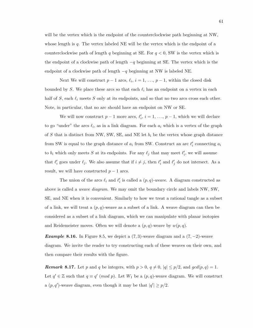
61
will be the vertex which is the endpoint of the counterclockwise path beginning at NW,
whose length is q. The vertex labeled NE will be the vertex which is the endpoint of a
counterclockwise path of length q beginning at SE. For q < 0, SW is the vertex which is
the endpoint of a clockwise path of length −q beginning at SE. The vertex which is the
endpoint of a clockwise path of length −q beginning at NW is labeled NE.
Next We will construct p− 1 arcs, `i, i = 1, . . ., p− 1, within the closed disk
bounded by S. We place these arcs so that each `i has an endpoint on a vertex in each
half of S, each `i meets S only at its endpoints, and so that no two arcs cross each other.
Note, in particular, that no arc should have an endpoint on NW or SE.
We will now construct p− 1 more arcs, `′i, i = 1, . . ., p− 1, which we will declare
to go “under” the arcs `i, as in a link diagram. For each ai which is a vertex of the graph
of S that is distinct from NW, SW, SE, and NE let bi be the vertex whose graph distance
from SW is equal to the graph distance of ai from SW. Construct an arc `′i connecting ai
to bi which only meets S at its endpoints. For any `j that may meet `′i, we will assume
that `′i goes under `j . We also assume that if i 6= j, then `′i and `′j do not intersect. As a
result, we will have constructed p− 1 arcs.
The union of the arcs `i and `′i is called a (p, q)-weave. A diagram constructed as
above is called a weave diagram. We may omit the boundary circle and labels NW, SW,
SE, and NE when it is convenient. Similarly to how we treat a rational tangle as a subset
of a link, we will treat a (p, q)-weave as a subset of a link. A weave diagram can then be
considered as a subset of a link diagram, which we can manipulate with planar isotopies
and Reidemeister moves. Often we will denote a (p, q)-weave by w(p, q).
Example 8.16. In Figure 8.5, we depict a (7, 3)-weave diagram and a (7,−2)-weave
diagram. We invite the reader to try constructing each of these weaves on their own, and
then compare their results with the figure.
Remark 8.17. Let p and q be integers, with p > 0, q 6= 0, |q| ≤ p/2, and gcd(p, q) = 1.
Let q′ ∈ Z such that q ≡ q′ (mod p). Let W1 be a (p, q)-weave diagram. We will construct
a (p, q′)-weave diagram, even though it may be that |q′| ≥ p/2.

62
NW
SESW
NE
(a) (7, 3)-weave.
NW
SE
NE
SW
(b) (7,−2)-weave.
Figure 8.5: Examples of weave diagrams.
Without loss of generality, suppose q′ ≥ p/2. A construction which is similar to the
following can be described for the case q′ ≤ −p/2. Construct the graph of the boundary
circle of the diagram as usual, and label the points NW and SE. Now, since q ≡ q′ (mod
p), q − q′ = np for some n ∈ Z. Note that since p > 0 and q′ > q, it must be that n < 0.
Thus we obtain q − np = q′, and note that −pn > 0. Now we want to label the vertices
SW and NE. Suppose q > 0. We travel counterclockwise from NW q edges, arriving at a
vertex we will label x. Now, from x, we travel counterclockwise −np more edges, arriving
at a vertex, y, after traveling a total of q − np = q′. Now, one trip around the boundary
circle requires traveling over 2p edges. Thus if n is even, we see that y = x. Thus We label
x as SW. We see that this is the same as the SW of W1, and thus we have constructed a
weave diagram which is identical to W1. If n is odd, then our trip ends on the opposite
half of the boundary circle. In this case we simply label y as NE instead, and again this
NE coincides with the NE of W1. Thus we have again constructed a weave diagram which
is identical to W1.
Similar arguments show that if q < 0 we will also construct a weave diagram which

63
is the same as W1. Thus a (p, q)- and (p, q′)-weave diagram are identical. So we will
always assume that |q| ≤ p/2.
We will now describe a sequence of Reidemeister moves on a (p, q)-weave diagram
which will reduce it into a different weave diagram, plus an additional crossing. The
location of this additional crossing in relation to the new weave will depend on the value
of q. Thus we will describe sequences for two cases: q > 0 and q < 0.
Let W be a (p, q)-weave. First suppose q > 0. Let a1 be the vertex on the
boundary circle that is adjacent to SE via a clockwise path, and let a2 be the other vertex
which is adjacent to SE. Let `1 denote the overstrand with endpoints at a1 and a2. Let `2
be the overstrand which is “to the left” of `1 in our weave diagram. Let `3 be the
understrand with endpoint at SE, and let α denote the crossing of `1 and `3. Finally, let
`4 be the overstrand with endpoint at NE, and let β denote the crossing of `3 and `4. See
Figure 8.6a for a weave diagram of the (5, 2)-weave, with the indicated labeling. Note that
for w(5, 2), `2 and `4 are the same strand.
The first move we make is a Type III Reidemeister move which pulls `2 from the
left side of α to the other side. This sets up a Type II Reidemeister move, in which we
pull `1 completely out from under `2. In the case of the (5, 2)-weave, as in Figure 8.6c,
this sets up another Type II Reidemeister move, which will pull `1 completely off of `3.
Finally, we perform a Type I move which will remove the crossing α. This results in NW
and SW being connected by a single arc.
In general, there may be more overstrands which we must pull `1 underneath to
set up this Type II move. In particular, we perform the Type III and Type II moves as
above for the |q| − 1 overstrands between `1 and the overstrand with endpoint at SW.
After moving these overstrands, the crossing β is exposed. When we perform the above
sequence of Reidemeister moves on a (p, q)-weave diagram, removing |q| − 1 overstrands
from the diagram and exposing a crossing, we say we have performed an un-weaving step.

64
NW
SE
SW
NE
a2
a1
`1`2
`3
α
β
(a)
NW
SE
SW
NE
`2
`1
`3
α
β
(b)
NW
SE
SW
NE
`2
`1
`3
α
β
(c)
NW
SE
SW
NE
`2
`1
`3
β
(d)
NW
SE
SW
NE
`2
`3
β
(e)
NW
SESW
NE
`2
`3
β
(f)
Figure 8.6: Performing an un-weaving step on a (5, 2)-weave.
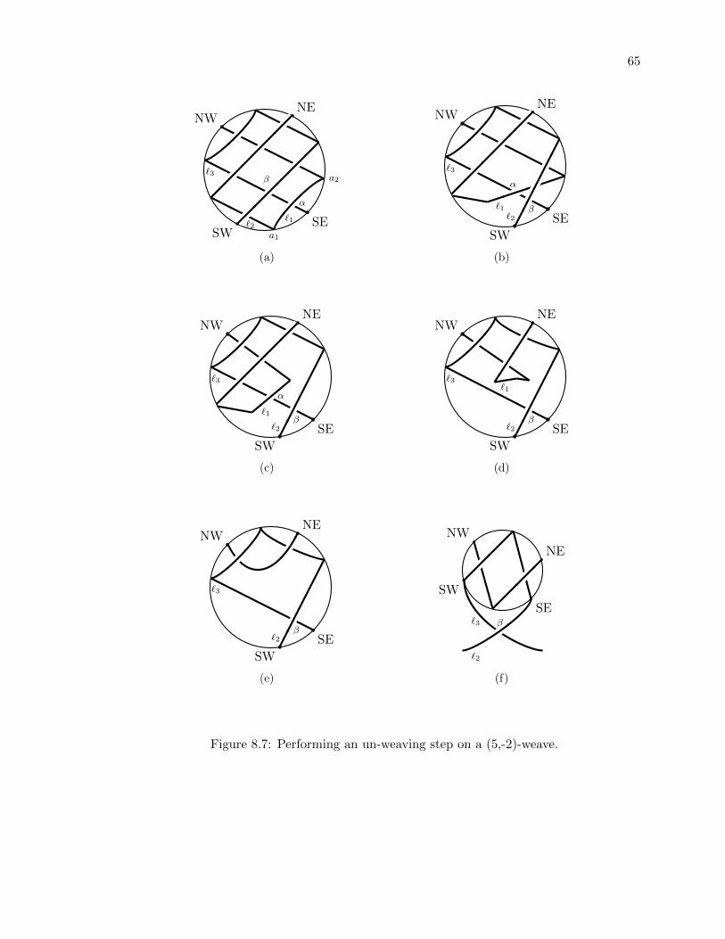
65
NW
SE
NE
SW a1
a2
`1
`3
`2
α
β
(a)
NW
SE
NE
SW
`1
`3
`2
α
β
(b)
NW
SE
NE
SW
`1
`3
`2
α
β
(c)
NW
SE
NE
SW
`1`3
`2β
(d)
NW
SE
NE
SW
`3
`2β
(e)
NW
SE
SW
NE
`3
`2
β
(f)
Figure 8.7: Performing an un-weaving step on a (5,-2)-weave.

66
In Figure 8.7, we show how to perform an un-weaving step on the weave w(5,−2).
Notice that instead of exposing a crossing to the right, we expose a crossing on the
bottom. In general, this will be the case for any weave w(p, q) with q < 0.
Notice that in Figure 8.6f, we have depicted the result of an un-weaving step on
the (5, 2)-weave as a (3,−1)-weave plus an integer tangle [1]. In particular, the result of
an un-weaving step on any (p, q)-weave includes a weave. We would like to determine
which weave we obtain via an un-weaving step. Suppose q > 0. The crossing we expose
via an un-weaving step is the crossing of the understrand `3 with endpoint at SE, and the
overstrand `2 with endpoint at NE. Let x be the endpoint of `3 which is not SE, and y be
the endpoint of `2 which is not NE. Then after performing an un-weaving step, we see
that x is the NE of the new weave, and y is the SE of the new weave. Now, there are q− 1
overstrands between `2 and the overstrand with endpoint at x. Thus the distance from SE
to NE in the new weave is q, since we travel along a path which hits exactly one endpoint
of each of the q − 1 overstrands, and ends at x. Also, NW and SW are unchanged when
we perform an un-weaving step, so the distance from NW to SW is still q. Then, since we
removed q− 1 overstrands, the new weave is a (p− q, q)-weave. Note that we may consider
the new weave as a (p− q, q − p)-weave if q > p−q2 .
In the case q < 0, we note that y will be on the opposite side of SE. After
performing an un-weaving step, y will be the SE of the new weave. Also, x will be the SW
of the new weave. There were −q − 1 overstrands between SW and SE in w(p, q). We
removed these overstrands, plus the overstrand `2 from the original weave. Thus the new
weave has p+ q − 1 overstrands. Notice that the offset does not change. So the new weave
is w(p+ q, q), if −p+q2 < q < 0.
We summarize our results about un-weaving a (p, q)-weave in the following lemma.
We recall, for emphasis, that any weave is a tangle.
Lemma 8.18. Let W be a (p, q)-weave.
(i) If q > 0, then performing an un-weaving step on W results in W ′ + [1], where W ′ is
a (p− q, q)-weave.
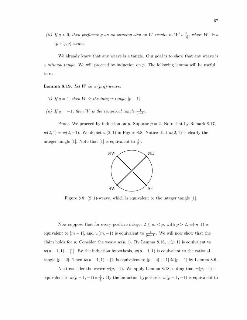
67
(ii) If q < 0, then performing an un-weaving step on W results in W ′ ? 1[1] , where W ′ is a
(p+ q, q)-weave.
We already know that any weave is a tangle. Our goal is to show that any weave is
a rational tangle. We will proceed by induction on p. The following lemma will be useful
to us.
Lemma 8.19. Let W be a (p, q)-weave.
(i) If q = 1, then W is the integer tangle [p− 1].
(ii) If q = −1, then W is the reciprocal tangle 1[p−1] .
Proof. We proceed by induction on p. Suppose p = 2. Note that by Remark 8.17,
w(2, 1) = w(2,−1). We depict w(2, 1) in Figure 8.8. Notice that w(2, 1) is clearly the
integer tangle [1]. Note that [1] is equivalent to 1[1] .
NW
SESW
NE
Figure 8.8: (2, 1)-weave, which is equivalent to the integer tangle [1].
Now suppose that for every positive integer 2 ≤ m < p, with p > 2, w(m, 1) is
equivalent to [m− 1], and w(m,−1) is equivalent to 1[m−1] . We will now show that the
claim holds for p. Consider the weave w(p, 1). By Lemma 8.18, w(p, 1) is equivalent to
w(p− 1, 1) + [1]. By the induction hypothesis, w(p− 1, 1) is equivalent to the rational
tangle [p− 2]. Then w(p− 1, 1) + [1] is equivalent to [p− 2] + [1] ∼= [p− 1] by Lemma 8.6.
Next consider the weave w(p,−1). We apply Lemma 8.18, noting that w(p,−1) is
equivalent to w(p− 1,−1) ? 1[1] . By the induction hypothesis, w(p− 1,−1) is equivalent to

68
the reciprocal tangle 1[p−2] . Then w(p− 1,−1) is equivalent to 1
[p−2] ?1[1]∼= 1
[p−1] by Lemma
8.6.
�
Since any integer or reciprocal tangle is rational, Lemma 8.19 implies that any
(p,±1)-weave is a rational tangle. When p = 2, this will give us our base case for our
induction. We now prove the general theorem.
Theorem 8.20. Let W be a (p, q)-weave.
(i) If q > 0, then W is equivalent to the rational tangle T with F (T ) = p−qq .
(ii) If q < 0, then W is equivalent to the rational tangle T with F (T ) = −qp+q .
Proof. We will proceed by induction on p. Note that the case p = 2 is a direct
result of Lemma 8.19. Next we suppose that for some positive integer p, for all 2 ≤ m < p,
(i) and (ii) hold for w(m, q) for any integer q such that gcd(m, q) = 1. We will show that
(i) and (ii) hold for w(p, q) for any q with gcd(p, q) = 1.
To prove (i), suppose q > 0 and gcd(p, q) = 1. We consider two cases: q ≤ p−q2 and
q > p−q2 . First suppose q ≤ p−q
2 . By Lemma 8.18, w(p, q) is equivalent to w(p− q, q) + [1].
Note that p− q < p and that gcd(p− q, q) = 1, so by the induction hypothesis, we have
F (w(p− q, q)) = (p−q)−qq = p−2q
q . Then by Lemma 8.11,
F (w(p− q, q) + [1]) = F (w(p− q, q)) + 1 =p− 2q
q+ 1 =
p− qq
.
For the second case, suppose q > p−q2 . Again, we have w(p, q) is equivalent to
w(p− q, q) + [1], but since q > p−q2 , we consider w(p− q, q) as
w(p− q, q − (p− q)) = w(p− q, 2q − p). Note in particular that 2q − p < 0, and that
gcd(p− q, 2q − p) = 1. By the induction hypothesis, we obtain
F (w(p− q, 2q − p)) =p− 2q
(p− q) + (2q − p)=p− 2q
q.

69
Again by Lemma 8.11,
F (w(p− q, 2q − p) + [1]) = F (w(p− q, 2q − p)) + 1 =p− 2q
q+ 1 =
p− qq
.
To prove (ii), suppose q < 0 and gcd(p, q) = 1. Again, we consider two cases:
q > p+q2 and q ≤ p+q
2 . First suppose q > p+q2 . Then by Lemma 8.18, w(p, q) is equivalent
to w(p+ q, q) ? 1[1] . By the induction hypothesis, we obtain
F (w(p+ q, q)) = −q(p+q)+q = −q
p+2q . Then
F
(w(p+ q, q) ?
1
[1]
)=
1
1 + 1F (w(p+q,q))
=1
1 + 1−q
p+2q
=1
1 + p+2q−q
=−q
−q + p+ 2q=−qp+ q
.
Finally, suppose q ≤ p+q2 . We know that w(p, q) is equivalent to w(p+ q, q). But
since q ≤ p+q2 , we take w(p+ q, q) to be w(p+ q, q + (p+ q)) = w(p+ q, p+ 2q). Note that
p+ q < p, and p+ 2q > 0. By the induction hypothesis, we obtain
F (w(p+ q, p+ 2q)) = p+q−(p+2q)p+2q = −q
p+2q . Then we have
F
(w(p+ q, p+ 2q) ?
1
[1]
)=
1
1 + 1F (w(p+q,p+2q))
=1
1 + 1−q
p+2q
=−qp+ q
.
�
Theorem 8.20 tells us that the class of weaves is contained in the class of rational
tangles. It turns out that a partial converse is also true. To prove this, we need to be able
to turn a given rational tangle into a weave. Since the process we described for
transforming a weave into a rational tangle involved only sequences of Reidemeister
moves, it is reversible. Thus, given w(p, q) + [1] or w(p, q) ? 1[1] , we can “weave in” the
extra crossing given to obtain a weave. We illustrate this process for the weave w(5, 2), in
Figure 8.9, and for w(5,−2) in Figure 8.10.
Lemma 8.21. Let W be a (p, q)-weave.
(i) If q > 0, then W + [1] is equivalent to w(p+ q, q).
70
(ii) If q > 0, then W ? 1[1] is equivalent to w(2p− q, q − p).
(iii) If q < 0, then W + [1] is equivalent to w(2p+ q, p+ q).
(iv) If q < 0, then W ? 1[1] is equivalent to w(p− q, q).
Proof. To prove (i), suppose q > 0. Note that there are q − 1 overpasses of W with
endpoints between SE and NE on the boundary circle. By weaving in the integer tangle
[1], which is attached to W at SE and NE, we will pull each of the q − 1 overpasses
through hte crossing at [1], by the sequence of Reidemeister moves outlined previously.
This will create q − 1 new overpasses, and an additional overpass from the over-crossing in
the integer tangle [1]. Thus we have obtained a weave W ′ with a total of
p− 1 + (q − 1) + 1 = p+ q − 1 overpasses. Then if W ′ = w(p′, q′), we have p′ = p+ q.
Notice that W ′ has q − 1 the distance from SE to NE, around the boundary circle of W ′,
is q. Then we see that q′ = q. Thus W ′ = w(p+ q, q).
Next we prove (ii). We notice that there are p− q − 1 overpasses of W with
endpoints between SE and NE on the boundary circle. When we perform a weaving step,
weaving in 1[1] , we pull each of these p− q − 1 overpasses through the crossing of 1
[1] . In
doing so, we create p− q − 1 new overpasses, plus an additional overpass from the
over-crossing of 1[1] . Thus we create p− q total new overpasses. So we have a new weave
W ′ = w(p′, q′) with a total of p− 1 + p− q = 2p− q − 1 overpasses. So p′ = 2p− q. Now,
in W ′ there are q + p− q − 1 = p− 1 overpasses with endpoints between NW and SW. So
we might expect that q′ = p. However, we have p > p− q2 = 2p−q
2 . Thus we take
q′ = p− (2p− q) = q − p. Thus W ′ = w(2p− q, q − p).
To see that (iii) holds, assume q < 0. In this case, there are p+ q − 1 overpasses of
W with endpoints between SE and NE on the boundary circle. To weave in the integer
tangle [1], we pull each of these overpasses through [1] by the same sequence of
Reidemeister moves as we did in (i). We obtain a new weave W ′. The weave W ′ has p+ q
more overpasses than W . We obtain p+ q − 1 of these overpasses from the p+ q − 1
overpasses of W which we performed the moves on, and we obtain an additional overpass

71
from the integer tangle [1]. Thus W ′ has p− 1 + (p+ q) = 2p+ q − 1 total overpasses. If
we suppose that W ′ = w(p′, q′), then it follows that p′ = 2p+ q.
Recall that in W , the distance from NW to NE, around the boundary circle, was
−q. In the weave W ′, the distance from NW to NE is −q + p+ q = p. So we might expect
that q′ = −p, giving W ′ = w(2p+ q,−p). However, since q < 0, we have −p < −(2p+q)2 .
Thus we take W ′ to be w(2p+ q,−p+ 2p+ q) = w(2p+ q, p+ q), as desired.
Finally, we prove (iv). In this case, there are −q − 1 overpasses with endpoints
between SE and SW. When we perform a weaving step, we pull these −q − 1 overpasses
through the crossing of 1[1] , creating −q − 1 new overpasses. The result of the weaving step
is a new weave W ′ = w(p′, q′) with a total of (p− 1)− q − 1 + 1 = p− q − 1 overpasses.
Thus p′ = p− q. Now, the weaving step had no effect on the number of overpasses with
endpoints between NW and NE, which is −q. Thus we see that q′ = q. So
W ′ = w(p− q, q). �
We can generalize Lemma 8.21 for general positive integer tangles and reciprocal
tangles.
Lemma 8.22. Let W be a (p, q)-weave, and n a positive integer.
(i) If q > 0, then W + [n] is equivalent to w(p+ nq, q).
(ii) If q > 0, then W ? 1[n] is equivalent to w(p(n+ 1)− nq, q − p).
(iii) If q < 0, then W + [n] is equivalent to w(p(n+ 1) + nq, p+ q).
(iv) If q < 0, then W ? 1[n] is equivalent to w(p− nq, q).
Proof. We can prove all four statements via induction on n. First suppose n = 1.
Then all four statements are true as a direct consequence of Lemma 8.21. Now suppose
that all four statements hold for some positive integer n. We will show that each
statement holds for n+ 1.
First we consider (i). We have w(p, q) + [n+ 1] ∼= w(p, q) + [n] + [1] ∼= w(p+ nq, q),
by the induction hypothesis. Then by Lemma 8.21, w(p+ nq, q) + [1] ∼= w(p+ (n+ 1)q, q).
72
For (ii), we have w(p, q) ? 1[n+1]
∼= w(p, q) ? 1[1] ?
1[n]∼= w(2p− q, q − p) ? 1
[n] by
Lemma 8.21. Then by the induction hypothesis, we have
w(2p− q, q − p) ? 1[n]∼= w(2p− q − n(q − p), q − p) = w(p(n+ 2)− (n+ 1)q, q − p).
To prove (iii) and (iv), we assume q < 0. For (iii), we have
w(p, q) + [n+ 1] ∼= w(2p+ q, p+ q) + [n] by Lemma 8.21. Then we have
w(2p+ q, p+ q) + [n] ∼= w(2p+ q + n(p+ q), p+ q) = w(p(n+ 2) + (n+ 1)q, p+ q) by the
induction hypothesis.
Finally, to prove (iv), we have w(p, q) ? 1[n+1]
∼= w(p− nq, q) ? 1[1] by the induction
hypothesis. Then by Lemma 8.21, we have
w(p− nq, q) ? 1[1]∼= w(p− nq − q, q) = w(p− (n+ 1)q, q).
Thus all four statements hold for n+ 1. We conclude by induction that all four
statements hold for all positive integers. �

73
NW
SESW
NE
(a)
NW
SESW
NE
(b)
NW
SESW
NE
(c)
NW
SESW
NE
(d)
NW
SESW
NE
(e)
NW
SE
SWNE
(f)
Figure 8.9: Performing a weaving step on a (5, 2)-weave, plus an additional crossing.

74
NW
SE
NE
SW
(a)
NW
SE
NE
SW
(b)
NW
SE
NE
SW
(c)
NW
SE
NE
SW
(d)
NW
SE
NE
SW
(e)
NW
SE
NE
SW
(f)
Figure 8.10: Performing a weaving step on a (5,-2)-weave.

75
Theorem 8.23. Let T be a rational tangle in canonical form
T = [a2n+1] +1
[a2n] + . . .+ 1[a2]+
1[a1]
,
and F (T ) = pq . Then T is equivalent to the weave w(p+ q, q).
Proof. We proceed by induction on n, or the number of terms in the continued
fraction of T . First suppose n = 0. Then T has only one term in its continued fraction
form, and is thus an integer tangle. Then q = 1, and by Lemma 8.19 T is equivalent to the
weave w(p+ 1, 1).
Now suppose that n > 0, and that the statement of the theorem holds for any
rational tangle with 2m+ 1 terms in continued fraction form, where 0 ≤ m < n.
Since T is in canonical form, we note that T is equivalent to (T ′ ? 1[a2n]
) + [a2n+1],
where T ′ is a rational tangle, in canonical form, with
T ′ = [a2n−1] +1
[a2n−2] + . . .+ 1[a2]+
1[a1]
.
Then choose integers p′ and q′ such that
p′
q′= a2n−1 +
1
a2n−2 + . . .+ 1a2+
1a1
.
Since T ′ has only 2n− 1 terms in its continued fraction form, the induction hypothesis
implies T ′ is equivalent to the weave w(p′ + q′, q′).
We notice that
p
q= a2n+1 +
1
a2n + 1a2n−1+
1
a2n−2+...+ 1
a2+1a1
= a2n+1 +1
a2n + 1p′q′
.
76
Then we obtain
a2n+1 +1
a2n + 1p′q′
= a2n+1 +p′
a2np′ + q′=a2na2n+1p
′ + a2n+1q′ + p′
a2np′ + q′.
We have
gcd(a2na2n+1p′ + a2n+1q
′ + p′, a2np′ + q′) = gcd(p′, q′) = 1,
so we obtain p = a2na2n+1p′ + a2n+1q
′ + p′ and q = a2np′ + q′.
We will now show that (T ′ ? 1[a2n]
) + [a2n+1] is equivalent to w(p+ q, q). First we
consider T ′ ? 1[a2n]
. Recall that T ′ ∼= w(p′ + q′, q′). Note that, since q′ < p′, we have
p′ + q′
2>q′
2+q′
2= q′.
Thus, by Lemma 8.22, part (ii),
w(p′ + q′, q′) ?1
[a2n]∼= w((p′ + q′)(a2n + 1)− a2nq′, q′ − (p′ + q′)) = w(a2np
′ + p′ + q′,−p′).
Now, since a2n ≥ 1, and p′ > q′ > 0, we have
a2np′ + p′ + q′
2>a2np
′ + p′
2≥ p′ + p′
2= p′.
Thus −p′ < a2np′+p′+q′
2 . Then by Lemma 8.22, part (iii), we have
w(a2np′+p′q′,−p′)+[a2n+1] ∼= w((a2p
′+p′+q′)(a2n+1+1)+a2n+1(−p′),−p′+a2n+ 1p′+p′+q′).
We notice that
(a2p′ + p′ + q′)(a2n+1 + 1) + a2n+1(−p′) = a2na2n+1p
′ + a2n+1q′ + p′ + a2np
′ + q′ = p+ q,
and that
−p′ + a2n+1p′ + p′ + q′ = a2np
′ + q′ = q.

77
Thus it follows that (T ′ ?
1
[a2n]
)+ [a2n+1] ∼= w (p+ q, q) .
�

78
CHAPTER 9
2-BUTTERFLIES AND RATIONAL LINKS
In this chapter, we will prove that the 2-bridge links coincide with a class of links
known as the rational links. We give a proof that utilizes butterflies and weaves. In
Chapter 8, we proved that every weave is a rational tangle, and that almost every rational
tangle is a weave (the rational tangles [0] and [∞], for instance, cannot be realized as
weaves as we have defined them). A rational link is a link obtained from a rational tangle
in a particular way. We will utilize our previous results to relate a link obtained from a
weave to a link obtained from a rational tangle, and vice-versa.
Definition 9.1. Let T be a rational tangle. We call the link obtained by connecting NW
to NE, and SW to SE, without creating new crossings, the numerator closure of T . We
call the link obtained by connecting NW to SW, and NE to SE, without creating new
crossings, the denominator closure of T . We denote the numerator and denominator
closures of T by N(T ) and D(T ), respectively. See Figure 9.1.
T T
N(T ) D(T )
Figure 9.1: Numerator and denominator closures of a rational tangle T .

79
Definition 9.2. Let L be a link. Suppose L is equivalent to the numerator closure of a
rational tangle T , with continued fraction form
T = [an] +1
[an−1] + . . .+ 1[a2]+
1[a1]
,
such that each ai is nonzero. Then we call L a rational link, and we denote L by its
Conway notation, [[a1 a2 . . . an]].
Note that, without loss of generality, we will only consider numerator closures of
rational tangles, since N(T ) = D(T r), and D(T ) = N(T r) [6].
Remark 9.3. Suppose L is a rational link with Conway notation [[a1 . . . an]]. Note that
in Definition 9.2, we require that each ai is a nonzero integer. Since L is the numerator
closure of a rational tangle T with
F (T ) =p
q= an +
1
an−1 + . . .+ 1a2+
1a1
,
it must be that p > q, if pq is in reduced form. This will be very important for us later on.
Furthermore, recall Remark 8.5 and Remark 8.13. In the Conway notation [[a1 . . .
an]], the integers ai alternate between corresponding to integer and reciprocal tangles.
Since we can always assume that the first tangle in T is horizontal, and since we assume n
is odd, the last tangle in T is horizontal. That is, both a1 and an correspond to integer
tangles.
Theorem 9.4. Let L1 = N(T1) and L2 = N(T2) be rational links. If T1 and T2 have
fractions which are equal, then L1 and L2 are equivalent.
There are necessary and sufficient conditions for the equivalence of two rational
links [6]. However, we defer discussion of this result until Chapter 10.
Now that we have defined what we mean by rational links, we discuss 2-butterflies.
Recall that a 2-butterfly consists of a graph R, which divides S2 = ∂B3 into two polygonal

80
faces, each of which contains an arc t, which we call a trunk. Each polygonal face, with its
trunk, is called a butterfly. We would like for our 2-butterfly diagrams to consist of a cycle
graph. That is, we would like every vertex of the butterfly graph to be bivalent. Consider,
for example, the 2-butterfly in Figure 9.2. This 2-butterfly contains a univalent B-vertex.
We note that this diagram can be transformed into a 2-butterfly in which each vertex is
bivalent via a Type I butterfly move.
Figure 9.2: 2-butterfly with a univalent B-vertex.
In fact, we can show that any 2-butterfly which contains a univalent B-vertex can
be transformed into a 2-butterfly in which every vertex is bivalent. The proof of this claim
is very similar to the proof of Theorem 7.1. Let B be a 2-butterfly, and let b1 be a
univalent B-vertex of B. Since b1 is univalent, it is connected to exactly one other vertex,
which we label x. Since the graph of B is bivalent, x is either an A-vertex or an E-vertex.
If x is an A-vertex, we can perform a Type I butterfly move, removing b1 and associated
edges. If x is an E-vertex, we can perform a Type II butterfly move, removing b1 and
associated edges. By inducting on the length of the path from b1 to the nearest
non-univalent B-vertex, we can show that B is equivalent to a 2-butterfly diagram in

81
which each vertex is bivalent. We leave it to the reader to compare to the proof of
Theorem 7.1 and fill in details.
Lemma 9.5. Let B = (R, T ) be a 2-butterfly diagram. Then B is equivalent to a
2-butterfly diagram in which each vertex is bivalent.
From now on, when we consider a 2-butterfly diagram, we will assume that each of
its vertices is bivalent.
Figure 9.3: This is not a 2-butterfly, since the trunks have coincident endpoints.
Let B = (R, T ) be a 2-butterfly diagram. Let n be the number of edges in R. By
Lemma 7.2, we know that n is divisible by 4. Let p ∈ Z such that n = 4p. If p = 1, then B
is as in Figure 9.3. Note that this fails to be a 2-butterfly, because the two trunks have
coincident endpoints. Thus we have proved the following lemma.
Lemma 9.6. Let B = (R, T ) be a 2-butterfly diagram. Then R has 4p edges, where p ≥ 2.
The simplest 2-butterfly diagram is the case where p = 2, as in Figure 9.4. In this
case, the butterfly graph is a cycle graph with 8 edges. The corresponding link of two
components is known as the Hopf Link.
Definition 9.7. Let B = (R, T ) be a 2-butterfly diagram. Suppose T = {t1, t2}, such that
t1 is the trunk of the bounded component. Fix an A-vertex a1 of t1. Let 2q denote the
minimum butterfly boundary distance from a1 to an A-vertex of t2, measured
counterclockwise. We call q the offset of B.

82
Figure 9.4: 2-butterfly diagram representing the Hopf Link.
Since the two trunks of a 2-butterfly diagram have distinct endpoints, the offset q
is always defined. Also, since R is bipartite, we have q ≥ 1. In the case of the 2-butterfly
diagram of Figure 9.4, the offset is q = 1.
Note that to construct a 2-butterfly diagram, all we need to do is (1) construct a
cycle graph with an acceptable number of edges, and (2) place the trunks. These two
steps correspond to picking an integer p so our graph has 4p edges, and choosing the offset
q. Thus we can associate to each 2-butterfly diagram an ordered pair (p, q).
Definition 9.8. Let B = (R, T ) be a 2-butterfly diagram. Suppose R contains 4p edges
and the offset of B is q, with 0 < q < p, and gcd(p, q) = 1. Then we call B a (p, q)
2-butterfly diagram.
Example 9.9. In Figure 9.5, we depict a (7, 3) 2-butterfly diagram. Notice that each
vertex is bivalent. Furthermore, the graph contains 14 B-vertices, 10 E-vertices, and 4
A-vertices. In general, a (p, q) 2-butterfly diagram will contain 2p B-vertices, 2p− 4
E-vertices, and 4 A-vertices.
Remark 9.10. In our definition of a (p, q) 2-butterfly, we require gcd(p, q) = 1. This
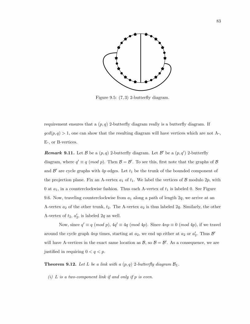
83
Figure 9.5: (7, 3) 2-butterfly diagram.
requirement ensures that a (p, q) 2-butterfly diagram really is a butterfly diagram. If
gcd(p, q) > 1, one can show that the resulting diagram will have vertices which are not A-,
E-, or B-vertices.
Remark 9.11. Let B be a (p, q) 2-butterfly diagram. Let B′ be a (p, q′) 2-butterfly
diagram, where q′ ≡ q (mod p). Then B = B′. To see this, first note that the graphs of B
and B′ are cycle graphs with 4p edges. Let t1 be the trunk of the bounded component of
the projection plane. Fix an A-vertex a1 of t1. We label the vertices of B modulo 2p, with
0 at a1, in a counterclockwise fashion. Thus each A-vertex of t1 is labeled 0. See Figure
9.6. Now, traveling counterclockwise from a1 along a path of length 2q, we arrive at an
A-vertex a2 of the other trunk, t2. The A-vertex a2 is thus labeled 2q. Similarly, the other
A-vertex of t2, a′2, is labeled 2q as well.
Now, since q′ ≡ q (mod p), 4q′ ≡ 4q (mod 4p). Since 4np ≡ 0 (mod 4p), if we travel
around the cycle graph 4np times, starting at a2, we end up either at a2 or a′2. Thus B′
will have A-vertices in the exact same location as B, so B = B′. As a consequence, we are
justified in requiring 0 < q < p.
Theorem 9.12. Let L be a link with a (p, q) 2-butterfly diagram BL.
(i) L is a two-component link if and only if p is even.

84
012
3
2q − 1
2q
2q + 1
2p− 5
2p− 4
2p− 3
2p− 2 2p− 12p2p+ 1 2p+ 2
2p+ 3
2p+ 2q − 1
2p+ 2q
2p+ 2q + 1
4p− 5
4p− 4
4p− 34p− 2
4p− 1
t1t2
Figure 9.6: A (p, q) 2-butterfly with its vertices labeled modulo 4p.
(ii) L is a knot if and only if p is odd.
Proof. First we will show that there are precisely two equivalence classes, under
the map p, of A- and E-vertices of BL. Let t1 and t2 be the trunks of BL. Fix an A-vertex
a1 of t1. We label the A- and E-vertices of BL modulo 2p, beginning with 0 at a1, in
ascending counterclockwise order. See Figure 9.7.
01
q
p− 2
p− 1 p p+ 1
p+ q
2p− 2
2p− 1
t1t2
Figure 9.7: A (p, q) 2-butterfly, with A- and E-vertices labeled modulo 2p.
We claim that the two equivalence classes of A- and E-vertices of BL, under the
85
equivalence relation ', are the sets of even and odd labeled vertices, respectively. Let A
be the set of A- and E-vertices of BL. Suppose x ' y. Then x and y are t1-equivalent, or x
and y are t2-equivalent. If x and y are t1-equivalent, then they are equidistant, via
butterfly boundary distance, from a1. Let 2d be the common distance of x and y to a1,
which is even since the butterfly graph is bipartite. Without loss of generality, we assume
that x is the endpoint of the counterclockwise path, starting at a1, with length 2d. We
will assume y is the endpoint of such a path, going clockwise. Then x is labeled d and y is
labeled 2p− d. If d is odd, then so is 2p− d. Thus x and y are both labeled as odd.
Similarly, if d is even, then both x and y are labeled as even.
A similar argument will show that if x and y are t2-equivalent, then they are both
labeled even or are both labeled odd.
Now let x ∈ A such that x is labeled as 2k. Let x′ ∈ A such that x′ is t1-equivalent
to x. Let 2d be the butterfly boundary distance of x to a1. Then the butterfly boundary
distance of x′ to a1 is also 2d. Thus we can construct a path of length 4d which starts at x
and ends x′. If this path goes clockwise, then 2k < p, and 2k = d. Then x′ is labeled as
d− 2d = −d, which is even. If the path goes counterclockwise, then 2k > p, and 2k ≡ −d
(mod 2p). Then x′ is labeled as −d+ 2d = d, which is even. Thus each vertex in the
equivalence class of x is labeled as even.
Similar arguments will prove the cases in which x is labeled as odd, and in which
x′ is t2-equivalent to x. We conclude that the equivalence classes under ' of vertices in A
are precisely the sets of even and odd labeled A- and E-vertices of BL.
To prove (i), suppose p is even. Let a1 be the A-vertex of t1 which is labeled as 0
as above, and a2 be the other A-vertex of t1. Note that a2 is labeled as p. Since p is even,
a1 and a2 belong to the same equivalence class. Thus t1 corresponds to a component of
the link L. Then t2 must also correspond to a component of L. Thus L is a
two-component link.
Now suppose L is a two-component link. Note that if we label the vertices as
before, a1 and a2 are still labeled as 0 and p, respectively. Since L is a two-component

86
link, t1 corresponds to a component of L. Thus a1 and a2 must belong to the same
equivalence class under '. Since a1 is labeled as 0, which is even, a2 must also be labeled
as even. Thus p is even.
To prove (ii), first suppose p is odd. Note that a1 is labeled as 0, and thus even,
and a2 is labeled as p, which is odd. Thus a1 and a2 are not members of the same
equivalence class under '. Thus L must be a one-component link. In other words, L is a
knot.
Conversely, suppose L is a knot. Then a1 and a2 do not belong to the same
equivalence class under '. Since a1 is labeled as 0, which is even, and a2 is labeled as p, it
must be that p is odd.
�
Theorem 9.13. Let B = (R, T ) be a (p, q) 2-butterfly diagram. Then B corresponds to
N(w(p, k) + [1]), where −p/2 < k < p/2 and k ≡ q (mod p).
(a) (5, 2) 2-butterfly on a sphere. (b) Pulling the trunks off of the sphere.
Figure 9.8: Turning a 2-butterfly into a weave.
Proof. Recall that R is a cycle graph embedded on S2 = ∂B3. The sphere is split
into two hemispheres, which make up the two butterflies of B. Let B1 and B2 be these two

87
butterflies. When we fold the wings of B1 and B2, we obtain a link L which is embedded
in S3. In particular, we imagine the arcs of the link L which are obtained as under-arcs
from the butterfly-link algorithm as embedded on the sphere S2. We imagine that the
over-arcs corresponding to the trunks of B1 and B2 come off of S2, being contained within
the unit ball.
We want to shift our perspective, from the center of the ball, to outside of it. We
instead imagine t1 and t2 as being contained outside of the unit ball, with the under-arcs
of L still being embedded on S2. Note in particular that each hemisphere of S2 contains
exactly p− 1 arcs of L. We arrange the structure so that, from our perspective, we are
looking down directly at the center of B1, with the graph R appearing as the equator of
the sphere. See Figure 9.8a.
NW
SW
SE
NE
Figure 9.9: Flattening the sphere, giving the numerator closure of w(5, 2) + [1].
Next we pull the two trunks, t1 and t2, away from the sphere. From our
persepctive, we want to pull them to the right. In doing so, we make so that t1 crosses
over t2 from our point of view. See Figure 9.8b. Next we flatten S2 down into a disk,
which we imagine is embedded in a plane. The p− 1 arcs from one hemisphere will now
appear to pass over the p− 1 strands of the other hemisphere. See Figure 9.9.

88
We can arrange this process so that t1 has endpoints at NW and SE of the disk,
and t2 has endpoints at NE and SW of the disk. Then each of the p− 1 under-arcs
contained in the disk has endpoints which are equidistant from SW of the disk, since its
endpoints come from E-vertices of B which are t2-equivalent. Furthermore, since the offset
of B is q, the distance around the boundary of the disk from NW to SW is q. Similarly,
the distance from SE to NE is q. Then we see that the disk contains a (p, q)-weave. Thus
the result of the process is N(w(p, q) + [1]). �
Theorem 9.14. Let L be a link with a (p, q) 2-butterfly diagram B. Then L = N(T ),
where T is a rational tangle with fraction F (T ) = pq .
Proof. By Theorem 9.13, we know that B corresponds to N(w(p, k) + [1]), where
−p/2 < k < p/2 and k ≡ q (mod p). If k > 0, then k = q. Thus
N(w(p, k) + [1]) = N(w(p, q) + [1]). By Theorem 8.20, w(p, q) + [1] is a rational tangle
with fraction
F (w(p, q) + [1]) = F (w(p, q)) + 1 =p− qq
+ 1 =p
q.
If k < 0, then k = q − p. Thus N(w(p, k) + [1]) = N(w(p, q − p) + [1]). Again by
Theorem 8.20, w(p, q − p) + [1] is a rational tangle with fraction
F (w(p, q − p) + [1]) = F (w(p, q − p)) + 1 =p− q
p+ (q − p)+ 1 =
p− qq
+ 1 =p
q.
�
We can prove a partial converse to Theorem 9.14. Its proof will rely on the fact
that we can turn N(w(p, q) + [1]) into a (p, k) 2-butterfly diagram, where k ≡ q (mod p),
and 0 < k < p. This transformation is obtained by reversing the process described in the
proof of Theorem 9.13. We leave the details to the reader.
Theorem 9.15. Let L = N(T ) be a rational link with F (T ) = pq . Then L has a (p, k)
2-butterfly diagram, where k ≡ q (mod p), and 0 < k < p.
Proof. Let T be a rational tangle, in canonical form, with F (T ) = pq , such that

89
L = N(T ). We will consider two cases: q < p2 and q > p
2 .
First suppose q < p2 . Then by Theorem 8.23, T be equivalent to the weave
w(p+ q, q). Thus L is equivalent to N(w(p+ q, q). Since q < p2 , we know q < p+q
2 . Thus
by Lemma 8.18, N(w(p+ q, q)) is equivalent to N(w(p, q) + [1]), which can be transformed
into a (p, q) 2-butterfly diagram, which corresponds to L.
Now suppose q > p2 . Again by Theorem 8.23, T is equivalent to the weave
w(p, q − p). Thus L is equivalent to N(w(p+ q, q)). Since p2 < q < p, we know
p2 + q < 2q < p+ q, from which we obtain p
4 + q2 < q < p+q
2 . Thus by Lemma 8.18,
N(w(p+ q, q)) is equivalent to N(w(p, q − p) + [1]). Note that we consider the weave as
w(p, q − p) since q > p2 . We can transform N(w(p, q − p) + [1]) into a (p, q) 2-butterfly as a
consequence of Remark 9.11. �

90
CHAPTER 10
FUTURE QUESTIONS
In this chapter, we address a few directions in which future research can take.
These include problems which we have thus far failed to resolve, in spite of much effort,
and problems which we have considered only briefly.
As noted in Remark 9.11, a (p, q) 2-butterfly is the same as any (p, q′) 2-butterfly,
with q ≡ q′ (mod p). This is related to a result which is known as Schubert’s Theorem.
Theorem 10.1. (Schubert’s Theorem) Let L1 = N(T1) and L2 = N(T2) be rational links
with F (T1) = pq and F (T2) = p′
q′ . Then L1 and L2 are equivalent as links if and only if
(i) p = p′
(ii) Either q ≡ q′ (mod p) or qq′ ≡ 1 (mod p).
The original proof of this theorem is due to Schubert [8], who showed that the
double-branched cover of a rational link is a lens space. He then used the classification of
lens spaces to obtain the statement of Theorem 10.1. Kauffman and Lambropoulou give a
combinatorial proof of Schubert’s Theorem in [6].
We have attempted to construct a proof of Schubert’s Theorem utilizing
butterflies, thus far to no avail. We are able to show that if p = p′ and q ≡ q′ (mod p),
then a (p, q) 2-butterfly and a (p′, q′) 2-butterfly are the same (this is the content of
Remark 9.11. We hope that obtaining a proof of Schubert’s Theorem which utilizes
butterflies may give us valuable insight into the classification of 3-bridge links.
The classification of 3-bridge links is an open problem. Hilden, Montesinos,
Tejada, and Toro (HMTT) tackle this problem in [4], although they do not achieve a
classification. They approach the problem using 3-butterfly diagrams. Similarly to how we
could, without loss of generality, consider only 2-butterfly diagrams in which each vertex
is bivalent, HMTT consider 3-butterfly diagrams in which there are no univalent vertices.

91
HMTT prove that each 3-butterfly diagram can be associated to a 3-tuple of
rational numbers, (p/n, q/m, s/l). They also prove some special cases of equivalence of
3-butterfly diagrams.
Theorem 10.2. (i) The 3-butterfly (p/n, q/m, s/l) is equivalent to the 3-butterflies
(q/m, s/l, p/n) and (s/l, p/n, q/m).
(ii) If s > q, then the 3-butterfly (p/n, q/m, s/l) is equivalent to (p/n′, s/l′, q/m′), where
n′ ≡ (n+ s− q) (mod p), m′ ≡ (m+ p− s) (mod q), and l′ ≡ (l + q − p) (mod s).
Notice that the statement of this theorem is similar to Shubert’s Theorem.
However, Theorem 10.2 does not provide both necessary and sufficient conditions for the
equivalence of two 3-butterfly diagrams. As of yet, no such conditions are known.

92
BIBLIOGRAPHY
[1] Burde, Gerhard and Zieschang, Heiner and Heusener, Michael, Knots, De Gruyter,
Berlin, 2014.
[2] Gordon, C. McA. and Luecke, J., “Knots are determined by their complements”, J.
Amer. Math. Soc., vol. 2, no. 2, pp.371-415, 1989.
[3] Hilden, Hugh Michael and Montesinos, Jose Marıa and Tejada, Debora Marıa and
Toro, Margarita Marıa, “A new representation of links: Butterflies”, arXiv:1203.2045,
2012.
[4] Hilden, Hugh Michael and Montesinos, Jose Marıa and Tejada, Debora Marıa and
Toro, Margarita Marıa, “On the classification of 3-bridge links”, Revista Colombiana
de Matematicas, vol. 46, no. 2, pp.113-144, 2012.
[5] Kauffman, Louis H. and Lambropoulou, Sofia, “On the classification of rational
tangles”, Adv. in Appl. Math., vol. 33, no. 2, pp.199-273, 2004.
[6] Kauffman, Louis H. and Lambropoulou, Sofia, “On the classification of rational
knots”, Enseign. Math. (2), vol. 49, no. 3-4, pp.357-410, 2003.
[7] Murasugi, Kunio, Knot theory & its applications, Translated from the 1993 Japanese
original by Bohdan Kurpita, Reprint of the 1996 translation [MR1391727], Birkhauser
Boston, Inc., Boston, MA, 2008.
[8] Schubert, Horst, “Knoten mit zwei Brucken”, Mathematische Zeitschrift, vol. 65,
pp.133-170, 1956.
[9] Stillwell, John, Classical topology and combinatorial group theory, 2nd edition,
Springer-Verlag, New York, 1993.
93
[10] Thurston, William P., Three-dimensional geometry and topology. Vol. 1, Princeton
Mathematical Series, vol. 35, Edited by Silvio Levy, Princeton University Press,
Princeton, NJ, 1997.