a supra-convergent finite difference scheme for the...

DOI: 10.1007/s10915-006-9122-8Journal of Scientific Computing, Vol. 31, Nos. 1/2, May 2007 (© 2007)

A Supra-Convergent Finite Difference Schemefor the Poisson and Heat Equations on IrregularDomains and Non-Graded Adaptive Cartesian Grids

Han Chen,1 Chohong Min,2 and Frederic Gibou3

Received March 30, 2006; accepted (in revised form) November 28, 2006; Published online March 31, 2007

We present finite difference schemes for solving the variable coefficient Poissonand heat equations on irregular domains with Dirichlet boundary conditions.The computational domain is discretized with non-graded Cartesian grids, i.e.,grids for which the difference in size between two adjacent cells is not con-strained. Refinement criteria is based on proximity to the irregular interfacesuch that cells with the finest resolution is placed on the interface. We samplethe solution at the cell vertices (nodes) and use quadtree (in 2D) or octree (in3D) data structures as efficient means to represent the grids. The boundary ofthe irregular domain is represented by the zero level set of a signed distancefunction. For cells cut by the interface, the location of the intersection point isfound by a quadratic fitting of the signed distance function, and the Dirichletboundary value is obtained by quadratic interpolation. Instead of using ghostnodes outside the interface, we use directly this intersection point in the discret-ization of the variable coefficient Laplacian. These methods can be applied in adimension-by-dimension fashion, producing schemes that are straightforward toimplement. Our method combines the ability of adaptivity on quadtrees/octreeswith a quadratic treatment of the Dirichlet boundary condition on the inter-face. Numerical results in two and three spatial dimensions demonstrate sec-ond-order accuracy for both the solution and its gradients in the L1 and L∞norms.

KEY WORDS: Poisson equation; heat equation; irregular domains; supra-convergence; non-graded adaptive Cartesian grids; quadtrees; octrees.

1 Computer Science Department, University of California, Santa Barbara, CA 93106, USA.2 Department of Mathematics, KyungHee University, 130–701, Seoul, Korea.3 Mechanical Engineering Department and Computer Science Department, University of

California, Santa Barbara, CA 93106, USA. E-mail: [email protected]

19

0885-7474/07/0500-0019/0 © 2007 Springer Science+Business Media, LLC

20 Chen, Min, and Gibou

1. INTRODUCTION

The Poisson and the heat equations are two of the fundamentalequations used in the modeling of diffusion dominated phenomena, rang-ing from electromagnetism to semi-conductor growth to fluid mechanics. Awide variety of approaches exist for solving the Poisson equation on irreg-ular domains. In [26] Peskin introduced the immersed boundary method,which uses a δ-function that smears out the solution on a thin finite bandaround the interface. Leveque and Li introduced the immersed interfacemethod [16], which is a second-order accurate numerical method designedto preserve the jump condition at the interface. In [22, 24], Mayo et al.proposed a fast method using boundary integral techniques. Based on theGhost Fluid Method of Fedkiw et al. [8], Liu et al. [18] developed a first-order accurate symmetric discretization of the variable coefficient Poissonequation in the presence of an irregular interface across which the variablecoefficient, the solution and its derivative may have jumps. Gibou et al.[11] introduced a second-order accurate symmetric discretization of thevariable coefficient Poisson equation in the case where Dirichlet boundaryconditions are imposed on the irregular domain. In this case, ghost valuesacross the interface are defined by linear extrapolation allowing standardcentral differencing formulas to be used when discretizing the Laplaciannear the interface. Third and fourth-order accurate schemes were later pro-posed in Gibou et al. [9] by defining ghost values with higher-order extrap-olations. In this case the corresponding linear system is non-symmetric butthe method produces accurate results for very coarse grids, making themethod extremely efficient. Jomaa and Macaskill [14] showed that in thecase where ghost values are defined by linear extrapolations, the error nearthe boundary is in general large compared to the error found for regu-lar domains. Defining ghost values by a quadratic extrapolation makes thelinear system non-symmetric, but leads to errors comparable with thoseobtained for a regular domain.

Many physical problems have different scales and more often thannot, only small portions of the computational domain require finer res-olution. In this case, uniform grids become inefficient in terms of mem-ory storage and CPU usage, and adaptive mesh strategies are usuallyadopted. Adaptive mesh strategies for elliptic partial differential equations,such as the Poisson equations, are often associated with the finite elementmethod (see, e.g., [7, 13]). Young et al. [35] introduced a finite elementmethod employing adaptive mesh refinements for second-order variablecoefficient elliptic equations using a cut-cell representation of irregulardomains. However, adaptive mesh refinement strategies for the finite ele-ment method can be complex in the case of irregular domains due to the

A Supra-Convergent Finite Difference Scheme 21

organization of the resulting data structure. In addition, special care mustbe taken for moving boundary problems in order to guarantee good meshquality (see, e.g., [31]).

Cartesian grids have the advantage of easier grid generation overunstructured grids, especially in three spatial dimensions. In [12], Johan-sen and Colella presented a cell-centered finite volume discretization tosolve the variable coefficient Poisson equation on irregular domains withDirichlet boundary conditions. They used a multigrid approach and ablock-grid algorithm related to the adaptive mesh refinement scheme ofBerger and Oliger [5]. McCorquodale et al. [23] presented a node-cen-tered finite difference approach to solving the variable coefficient Poissonequation with Dirichlet boundary conditions on irregular domains usingthe block-structured adaptive mesh refinement and the multigrid solver ofAlmgren et al. [2–4]. Numerical evidence in [23] showed that while bothlinear and quadratic interpolations produce second-order accurate solu-tions, only quadratic interpolations (Shortley–Weller approximation [32])yield second-order accurate gradients in the L∞ norm. These methods,however, do not consider non-graded adaptive grids in which the differ-ence in size between two adjacent cells is not constrained.

Aftomis et al. [1] pointed out that quadtree/octree data structures (see,e.g., [29, 30] for an introduction on quadtree/octree data structures) couldbe used as an efficient means to represent Cartesian grids. Popinet [27]proposed a second-order non-symmetric numerical method to study theincompressible Navier–Stokes equations using an octree data structure torepresent the spatial discretization. In this method, a Poisson equation forthe pressure is solved to account for the incompressibility condition usinga standard projection method. Only graded trees, i.e., trees for which theratio between two adjacent cell sizes cannot exceed two, were consideredin [27]. Non-graded grids generate less nodes leading to efficient methodsand allow for more flexible grid generations since the size between adja-cent cells is not constrained. In [20], Losasso et al. proposed a first-orderaccurate symmetric discretization of the Poisson equation on non-gradedoctrees in the context of free surface flows. This work was then extendedto second-order accuracy in [19] using the work of Lipnikov et al. [17]. Acommon criticism of quadtree/octree data structures is the time it takes totraverse the tree from the root to a leaf. This issue can be alleviated byusing a uniform grid at the coarsest level and a quadtree/octree in everycell of this uniform grid as demonstrated in [19].

Recently, Min et al. [25] introduced a supra-convergent finite differ-ence scheme for solving the variable coefficient Poisson equation on reg-ular domains using non-graded grids represented by quadtrees/octrees.A hallmark of this method is that it produces second-order accurate


solutions with second-order accurate gradients (supra-convergence). In thispaper, we extend this method to solve the variable coefficient Poisson andthe heat equations on irregular domains. We describe the interface by theset of points where a level set function is zero. We automatically constructnon-graded Cartesian grids based on the proximity to the interface, i.e., weimpose the finest resolution at the interface. Such grid generations yieldstraightforward approximations of both the Poisson and the heat equa-tions on non-graded Cartesian meshes. We note, however, that one can inaddition refine the mesh in other regions if needed, as shown in Sec. 5.For interior nodes, the variable coefficient Laplacian is discretized as in[25], where the spurious error induced by interpolation at ghost nodes atT-junctions is cancelled out by a weighted combination of the discretiza-tions in other Cartesian directions. For nodes adjacent to the interface, thelocation of the interface point is found by a quadratic fitting of the signeddistance level set function, and the Dirichlet boundary value is obtainedeither explicitly (if an analytic formula is known) or calculated using aquadratic interpolation using neighboring nodal values in the case wherethe Dirichlet boundary values are defined at the nodes. The Shortley–Weller approximation [32], based on quadratic extrapolation, is then usedto discretize the Laplacian. The resulting non-symmetric linear system issolved using the stabilized bi-conjugate gradient (Bi-CGSTAB) methodwith the incomplete LU preconditioner [28]. In the case of the heat equa-tion, the Crank–Nicolson scheme is used with a time step of ∆t = c∆x,where 0<c<1 and ∆x is the size of the smallest cell. Numerical examplesdemonstrate that our method produces second-order accuracy for the solu-tion as well as its gradients in the L1 and L∞ norms. We emphasize thatsecond-order accuracy for the gradient is particularly important in Stefan-type problems since the overall accuracy of the method is determined bythe accuracy of the gradients at the interface. We find that our method onadaptive grids favorably compares to the symmetric solver of Gibou et al.[11] on uniform grids.

2. EQUATIONS

2.1. Poisson Equation

Consider a Cartesian computational domain, Ω, with exterior bound-ary, ∂Ω, and a lower-dimensional irregular interface, Γ , which divides thecomputational domain into disjoint pieces, the interior region Ω− and theexterior region Ω+ (see Fig. 1). The regions are represented by a level setfunction φ, taken to be the signed distance function to the interface Γ .That is, Ω− is represented by the set of points where φ < 0 and Ω+ is


Fig. 1. Schematic of two distinct regions Ω− and Ω+, separated by an interface Γ .

represented by the set of points where φ >0, whereas Γ is represented bythe set of points where φ = 0 The variable coefficient Poisson equation iswritten as

∇ · (ρ(x)∇u(x))=f (x), x ∈Ω, (1)

where ∇ = ( ∂∂x

, ∂∂y

, ∂∂z

) is the gradient operator and where ρ(x) is assumedto be continuous on each of the disjoint subdomains, Ω− and Ω+,but may be discontinuous across the interface Γ . Furthermore, ρ(x) isassumed to be bounded from below by a positive constant. On ∂Ω, eitherDirichlet or Neumann boundary conditions are specified. On the interfaceΓ , a Dirichlet boundary condition of uΓ =g(x) is specified. Thus, Eq. (1)decouples into two distinct equations, one on Ω− and one on Ω+, andthe solutions can be obtained independently.

2.2. Heat Equation

Ignoring the effects of convection, the standard heat equation reads

ρcvTt =∇ · (k∇T ), (2)

where T is the temperature, ρ the density, cv the specific heat at constantvolume, and k is the thermal conductivity. Assuming that ρ and cv are


constant allows Eq. (2) to be written as

Tt =∇ · (k∇T ), (3)

where k = kρcv

.

3. SPATIAL DISCRETIZATION ON QUADTREES/OCTREES

The computational domain Ω is discretized into squares (in 2D) orcubes (in 3D), and quadtree (in 2D) or octree (in 3D) data structuresare used to represent this discretization. As depicted in Fig. 6 for a 2Ddomain, the entire domain is originally associated with the root of thetree, which has a level of zero by definition. Then this discretization pro-ceeds recursively, i.e., each cell can be in turn split into four children whichhave one more level than their parent cell. A cell with no children is calleda leaf. Two cells are called neighbors if they share a common face or partof a face. The interested reader is referred to [29, 30] for more details onquadtree and octree data structures (Fig. 2).

By definition, a quadtree is graded if the difference between two adja-cent cell levels is at most one. In this paper, we sample the solution atthe nodes (vertices of cells) and we consider non-graded Cartesian grids,i.e., grids for which the level difference between two adjacent cells is notconstrained. In our non-graded Cartesian grids, a node is regular if it islinked to another node by a cell edge in each of the directions. In two

Fig. 2. Discretization of a 2D domain (left) and its quadtree representation (right). Theentire domain corresponds to the root of the tree (level 0), and each cell is subdivided intofour children, in the order of lower-left, upper-left, lower-right, upper-right. In this example,the tree is not graded since the difference of levels between neighboring cells exceeds one.


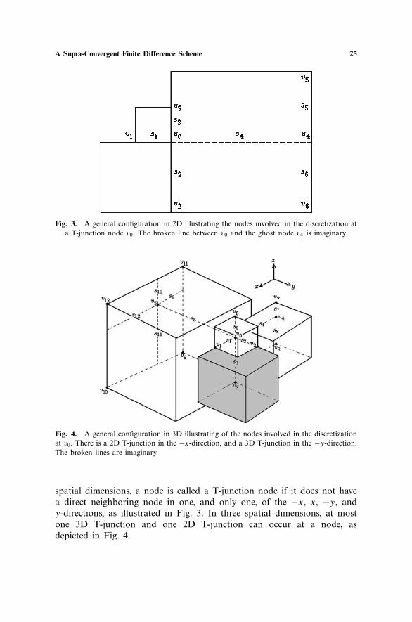
Fig. 3. A general configuration in 2D illustrating the nodes involved in the discretization ata T-junction node v0. The broken line between v0 and the ghost node v4 is imaginary.

Fig. 4. A general configuration in 3D illustrating of the nodes involved in the discretizationat v0. There is a 2D T-junction in the −x-direction, and a 3D T-junction in the −y-direction.The broken lines are imaginary.

spatial dimensions, a node is called a T-junction node if it does not havea direct neighboring node in one, and only one, of the −x, x, −y, andy-directions, as illustrated in Fig. 3. In three spatial dimensions, at mostone 3D T-junction and one 2D T-junction can occur at a node, asdepicted in Fig. 4.


Adaptive grids are usually generated in such a way as to produce auniform error throughout the entire domain, see, e.g., [34] for adaptivemesh generations based on a posteriori error estimate. For many problems,e.g., Stefan-type problems [6, 10], the solution’s gradient at the interfacedrives the interface motion and therefore the accuracy of the method. It istherefore desirable to discretize the computational domain in such a waythat the cell size is proportional to the distance to the interface. In thiswork, we split a cell c if the following test is satisfied:

minv∈V

|φ(v)|< lip×diag2

, (4)

where v is a vertex of the current cell c, V the set of all vertices of c, lipthe Lipschitz constant associated with φ, and diag is the diagonal lengthof the current cell. As pointed out by Strain in [33], this is a splitting algo-rithm that automatically generates non-graded Cartesian grids and guaran-tees the finest resolution on the interface. In addition, enforcing uniformcells with the smallest size on the interface prevents the occurrence ofT-junctions. This greatly simplifies our finite difference discretization inSec. 4.2 and allows a straightforward extension of the method of Minet al. [25].

4. FINITE DIFFERENCE SCHEMES

4.1. Variable Coefficient Poisson Equation on Regular Domains

We first recall the finite difference discretization from Min et al. [25]for the variable coefficient Poisson Eq. (1) on regular domains.

4.1.1. One Spatial Dimension

In one spatial dimension, the finite difference discretization on a non-uniform grid at a grid node xi is(

ui+1 −ui

si+ 1

2

· ρi+1 +ρi

2+ ui−1 −ui

si− 1

2

· ρi−1 +ρi

2

)· 2si+ 1

2+ s

i− 12

=fi +si+ 1

2− s

i− 12

3·uxxx +O(h2), (5)

where si− 1

2=xi −xi−1 and h=maxi si+ 1

2. Even though this scheme appears

to be second-order accurate only in the case where the grid is uniform, itis in fact second-order accurate (see, e.g., [15, 21]).


4.1.2. Two Spatial Dimensions

In two spatial dimensions, a node is either a regular node or aT-junction node, i.e., a node with a missing direct neighboring node. Weemphasize that the T-junction can only occur at one of the −x, +x, −y,and +y-directions. Let us consider the finite difference discretization fora T-junction node without a direct right neighboring node as depicted inFig. 3 noting that the discretization when the T-junction is in the otherdirections can be derived in a similar manner: denote by ui the solutionvalue at node vi . The ghost value u4 is calculated by linear interpolationusing u5 and u6:

u4 = s5u6 + s6u5

s5 + s6. (6)

The forward difference for ρux at node v0 is also linearly interpolated as

(ρux)+∣∣

v0= s5D6 + s6D5

s5 + s6, (7)

where

D5 = u5 −u0

s4· ρ5 +ρ0

2, (8)

D6 = u6 −u0

s4· ρ6 +ρ0

2. (9)

The discretizations for (ρux)x and (ρuy)y at the node v0, along with theirTaylor series expansions, are given by

(u1 −u0

s1· ρ1 +ρ0

2+ s6D5 + s5D6

s5 + s6

)· 2s1 + s4

= (ρux)x + s5s6

(s1 + s4)s4

(ρuy

)y+O(h) (10)

and

(u2 −u0

s2· ρ2 +ρ0

2+ u3 −u0

s3· ρ3 +ρ0

2

)· 2s2 + s3

= (ρuy

)y+O(h), (11)

respectively, where D5 and D6 are given by Eqs. (8) and (9). The spuri-ous term s5s6

(s1+s4)s4

(ρuy

)y

is due to the T-junction, and can be canceled by


appropriately weighting Eqs. (10) and (11) as:(u1 −u0

s1· ρ1 +ρ0

2+ s6D5 + s5D6

s5 + s6

)· 2s1 + s4

+(

u2 −u0

s2· ρ2 +ρ0

2+ u3 −u0

s3· ρ3 +ρ0

2

)

· 2s2 + s3

·(

1− s5s6

(s1 + s4)s4

)=f0 +O(h). (12)

Although this scheme appears to be first-order accurate, it is indeed sec-ond-order accurate as in the one spatial dimension. Not surprisingly, thisweighted scheme (12) reduces to the usual five point scheme in the case ofa regular node:(

u1−u0

s1· ρ1+ρ0

2+u4−u0

s4· ρ4+ρ0

2

)· 2s1+s4

+(

u2−u0

s2· ρ2+ρ0

2+u3−u0

s3· ρ3+ρ0

2

)· 2s2+s3

=f0+O(h), (13)

where v4 is the direct neighboring node of v0 to the right.

4.1.3. Three Spatial Dimensions

In three spatial dimensions, more complex configurations can occurdue to the adaptive nature of the Cartesian grid. The most general case isdepicted in Fig. 4, where one 2D T-junction in the −x-direction and one3D T-junction in the −y-direction are present. We emphasize that this isthe most general case and that no other T-junctions can occur at a singlenode. In this case two ghost values u4 and u5 are linearly interpolated as:

u4 = u7s8 +u8s7

s8 + s7(14)

and

u5 = u11s11s12 +u12s11s9 +u9s10s12 +u10s10s9

(s11 + s10)(s9 + s12). (15)

The backward difference (ρux)− and (ρuy)

− at node v0 are also linearlyinterpolated as

(ρux)− = ρ7 +ρ0

2· u7 −u0

s4· s8

s8 + s7+ ρ8 +ρ0

2· u8 −u0

s4· s7

s8 + s7(16)


and

(ρuy)− = ρ11 +ρ0

2· u11 −u0

s5· s11s12

(s11 + s10)(s9 + s12)

+ ρ12 +ρ0

2· u12 −u0

s5· s11s9

(s11 + s10)(s9 + s12)

+ ρ10 +ρ0

2· u10 −u0

s5· s10s9

(s11 + s10)(s9 + s12)

+ ρ9 +ρ0

2· u9 −u0

s5· s10s12

(s11 + s10)(s9 + s12), (17)

respectively.The discretizations for (ρux)x , (ρuy)y , and (ρuz)z at the node v0,

along with their Taylor series expansions, are given by

(ρ1 +ρ0

2· u1 −u0

s1− (ρux)

−)

2s1 + s4

= (ρux)x + s7s8

s4(s1 + s4)(ρuz)z +O(h),

(18)(ρ2 +ρ0

2· u2 −u0

s2− (ρuy)

−)

2s2 + s5

= (ρuy

)y+ s9s12

s5(s2 + s5)(ρux)x

+ s10s11

s5(s2 + s5)(ρuz)z +O(h) (19)

and

(ρ3 +ρ0

2· u3 −u0

s3+ ρ6 +ρ0

2· u6 −u0

s6

)2

s3 + s6= (ρuz)z +O(h), (20)

respectively, where (ρux)− and (ρuy)

− are given by Eqs. (16) and (17).As in two spatial dimensions, a linear combination of Eqs. (18)–(20)allows for the cancellation of the spurious errors terms s7s8

s4(s1+s4)(ρuz)z,

s9s12s5(s2+s5)

(ρux)x , and s10s11s5(s2+s5)

(ρuz)z, yielding the following scheme:

(ρ1 +ρ0

2· u1 −u0

s1+ (ρux)

−)

2s1 + s4

·α

+(

ρ2 +ρ0

2· u2 −u0

s2+ (ρuy)

−)

2s2 + s5

+(

ρ3 +ρ0

2· u3 −u0

s3+ ρ6 +ρ0

2· u6 −u0

s6

)2

s3 + s6·β =f0 +O(h)

(21)


with

α = 1− s10s11

s5(s2 + s5),

β = 1− s9s12

s5(s2 + s5)−α

s7s8

s4(s1 + s4). (22)

Although this scheme appears to be first-order accurate, it is in fact sec-ond-order accurate as it is in the 1D case. Not surprisingly, this weightedscheme (21) reduces to the usual seven point scheme in the case of a reg-ular node:(

u1 −u0

s1· ρ1 +ρ0

2+ u4 −u0

s4· ρ4 +ρ0

2

)· 2s1 + s4

+(

u2 −u0

s2· ρ2 +ρ0

2+ u5 −u0

s5· ρ5 +ρ0

2

)· 2s2 + s5

+(

u6 −u0

s6· ρ6 +ρ0

2+ u3 −u0

s3· ρ3 +ρ0

2

)· 2s6 + s3

=f0 +O(h),

(23)

where v4 and v5 are the direct neighbors of v0 in the −x and −y-directions.

4.2. Discretization Near the Interface

In the case where one or more of the neighboring nodes involved inthe spatial discretization, e.g., v1–v3, v5, v6 in Fig. 3 or v1–v3, v6–v12 inFig. 4, are outside the irregular domain (i.e., φ is positive), the interfaceintersects between the node v0 and the neighboring node(s). By enforcinga band of uniform cells along the interface, we guarantee that only uni-form cells are cut by the interface, and in this case v0 is a regular node.Let’s consider the 1D case, as depicted in Fig. 5, in which the interfaceintersects between v0 and v4 at vI. Denote by sI the distance between vIand v0. sI is approximated by finding the zero crossing of the quadratic

Fig. 5. v0 is a regular node and the interface Γ intersects between v0 and v4 at vI.


interpolant φ =φ0 +φxs + 12φxxs

2, where φ is the signed distance level setfunction. Since v1 and v0 are inside the irregular domain with negativevalues in φ and v4 is outside with a positive φ, the quadratic interpolantin φ is convex with a positive φxx , and sI is calculated as:

sI =

−φx +√

φ2x −2φxxφ0

φxx

, if φxx >ε,

−φ0

φx

if |φxx | ε,

(24)

where ε is a small positive number to avoid division by zero. φx and φxx

are approximated at v0 using central difference schemes:

φx =s1

φ4−φ0s4

+ s4φ0−φ1

s1

s1 + s4(25)

and

φxx =(

φ4 −φ0

s4− φ0 −φ1

s1

)2

s1 + s4. (26)

These schemes (25) and (26) are second-order accurate because of thelocally uniform grid spacing near the interface.

Once we know the location of the interface point, the Dirichletboundary value uI and ρI are either calculated with an analytic expres-sion or by quadratic interpolation using neighboring nodal values. Thenthe standard central difference scheme is used to approximate (ρux)x :

(ρux)x =(

uI −u0

sI· ρI +ρ0

2− u0 −u1

s1· ρ1 +ρ0

2

)· 2sI + s1

. (27)

When the interface intersects between the node and its neighboring nodesin any of the other directions, the discretization can be performed inde-pendently in a similar manner, which makes the method straightforward toimplement in a dimension-by-dimension framework. In addition, the qua-dratic interpolation near the interface prevents that the largest error besystematically located near the interface, as pointed out in [14, 23] andguarantees second-order accuracy for both the solution and its gradients.The resulting non-symmetric linear systems are diagonally dominant.

4.3. Heat Equation

We consider only the constant coefficient heat equation:

Tt =k∆T, (28)


noting that extension to the variable coefficient heat equation is straight-forward. Explicit schemes impose a time step restriction of ∆t (θ∆x)2

2kfor

stability, where ∆x is the size of the smallest cell and θ is the smallestcell fraction for cells cut by the interface. Since θ can be arbitrarily small,so is the time step restriction ∆t , which leads to unpractical schemes.Implicit schemes avoid such time step restrictions. We use the Crank–Nicolson scheme to discretize the heat Eq. (28):(

I − 12∆tk∆

)T n+1 =

(I + 1

2∆tk∆

)T n, (29)

where I is the identity matrix and T n is the solution at the nth time step.The spatial discretization of the Laplace operator in Secs. 4.1 and 4.2, isused to approximate ∆T . Since the Crank–Nicolson scheme (29) is uncon-ditionally stable and second-order accurate we choose a time step ∆t pro-portional to ∆x.

4.4. Computing Second-Order Accurate Gradients

To compute the gradients to second-order accuracy when T-junctionsare present, the ghost values u4 in Fig. 3 and u4, u5 in Fig. 4 are linearlyinterpolated as in Eqs. (6), (14), and (15). The spurious error caused bythe interpolation is successfully removed and the gradients are computedin 2D (following the notations in Fig. 3) as:

ux = u4 −u0

s4· s1

s1 + s4+ u0 −u1

s1· s4

s1 + s4− s5s6s1

2s4(s1 + s4)uyy,

(30)uy = u3 −u0

s3· s2

s2 + s3+ u0 −u2

s2· s3

s2 + s3,

where

uyy =(

u3 −u0

s3+ u2 −u0

s2

)· 2s2 + s3

.

Following the notations in Fig. 4, the gradients in 3D are calculated as:

ux = u1 −u0

s1· s4

s1 + s4+ u0 −u4

s4· s1

s1 + s4+ s7s8

2s4· s1

s1 + s4·uzz,

uy = u2 −u0

s2· s5

s2 + s5+ u0 −u5

s5· s2

s2 + s5+ s9s12

2s5· s2

s2 + s5·uxx

+ s10s11

2s5· s2

s2 + s5·uzz,

uz = u6 −u0

s6· s3

s3 + s6+ u0 −u3

s3· s3

s3 + s6, (31)


where uxx , uyy , and uzz are given by solving Eqs. (18)–(20) simultaneously.In the case where v0 is a regular node, Eqs. (31) and (31) reduce to theusual weighted average forward and backward differences:

ux = u4 −u0

s4· s1

s1 + s4+ u0 −u1

s1· s4

s1 + s4,

uy = u3 −u0

s3· s2

s2 + s3+ u0 −u2

s2· s3

s2 + s3(32)

in 2D, and

ux = u1 −u0

s1· s4

s1 + s4+ u0 −u4

s4· s1

s1 + s4,

uy = u2 −u0

s2· s5

s2 + s5+ u0 −u5

s5· s2

s2 + s5,

uz = u6 −u0

s6· s3

s3 + s6+ u0 −u3

s3· s6

s3 + s6(33)

in 3D. For nodes next to the interface, interface nodes are used in Eqs.(32) and (33) instead of those neighboring nodes that are outside thedomain. We note that the calculation of the gradient involves the samecells as those used in the discretization of the Poisson or heat equation,hence preserving the locality and ease of implementation of the method.

5. EXAMPLES

In this section, we present numerical evidence that confirms theschemes described in this paper produce second-order accuracy in the L1

and L∞ norms for both the solution and its gradients. We use meshesfor which the difference of level between adjacent cells can be greaterthan one, illustrating the fact that the method is supra-convergent on non-graded adaptive grids. The linear systems of equations are solved using thestabilized bi-conjugate gradient (Bi-CGSTAB) method with an incompleteLU preconditioner (see, e.g., [28]). In these examples, we solve the pois-son or heat equation on Ω− only, noting that the procedure to obtainthe solution on Ω+ is similar. We denote by min resoln and max resolnthe minimum and maximum grid resolution corresponding to the coars-est and finest cells in the grid, respectively. Specifically, if the cell size isdenoted by ∆x, then ∆x = L/min resoln for the coarsest cell and ∆x =L/max resoln for the finest cell, where L is the length of the computa-tional domain. In the following examples, we start with an initial adaptivegrid, e.g., with (min resoln, max resoln)=(16,128), and then recursivelysplit each cell into four (in 2D) or eight cells (in 3D), which effectively


increases min resoln and max resoln by one, to obtain the convergencetest results for the solution and its gradients. Other starting values of(min resoln, max resoln) can also be used to obtain similar results. Wealso assume the variable coefficients and the Dirichlet boundary values aredefined on grid nodes. Therefore, the variable coefficients and the Dirichletboundary values on the interface points are calculated by quadratic inter-polation using neighboring nodal values.

5.1. Poisson Equation

5.1.1. Example 1

Consider ∇ · (ρ∇u) = f on Ω = [−1,1] × [−1,1] with an exact solu-

tion of u=e10(x2+y2 −0.752), where ρ =1. The interface is a circle on whichφ =

√x2 +y2 −0.75=0. In this example, large solution gradients exist near

the circular interface where we impose the finest grid resolution, while thesolution near the center is smoother, where we can impose coarser gridresolution. We generate the adaptive grids by proximity to the interface,as described by the criterion in (4). Figure 6 depicts the adaptive Carte-sian grid with (min resoln, max resoln) = (16, 64), as well as the inter-face. The numerical solution on this grid is plotted in Fig. 7. Numerical

Fig. 6. Domain Ω = [−1,1] × [−1,1] and the spatial discretization in example 5.1.1 with(min resoln, max resoln) = (16, 64).


–1

–0.5

0

0.5

1

–1

–0.5

0

0.5

1

0.20.40.60.8

xy

u

Fig. 7. Graph of the solution in example 5.1.1, where (min resoln, max resoln) = (16, 64).The dots represent the approximate solution and the mesh represents the exact solution.

Table I. Accuracy Results for the Solution u in Example 5.1.1

(min resoln, max resoln) L∞ error Order L1 error Order

(32,128) 6.042×10−2 – 1.948×10−2 –(64,256) 1.673×10−2 1.852 5.136×10−3 1.924(128,512) 4.279×10−3 1.968 1.292×10−3 1.991(256,1024) 1.075×10−3 1.993 3.226×10−4 2.001

accuracy test results for the solution and its gradients are given in TablesI and II, respectively.

In many applications (e.g., Stefan type of problems), high-orderaccuracy of the solution’s gradients at the interface is desired. In thisexample, numerical accuracy test is also performed for the gradient at

Table II. Accuracy Results for the Solution’s Gradients ∇u in Example 5.1.1


(16,128) 6.676×10−1 – 3.897×10−1 –(32,256) 2.014×10−1 1.729 1.065×10−1 1.872(64,512) 5.713×10−2 1.818 2.739×10−2 1.959(128,1024) 1.581×10−2 1.853 6.914×10−3 1.986


Table III. Accuracy Results for the Solution’s Gradients ∇u on the Interface in Example 5.1.1


(16,64) 2.749 – 1.260 –(32,128) 9.751×10−1 1.495 3.977×10−1 1.663(64,256) 2.949×10−1 1.725 9.719×10−2 2.033(128,512) 8.145×10−2 1.857 2.568×10−2 1.920

the interface, which is obtained by second-order extrapolation of thegradient from Ω− to Ω+ followed by quadratic interpolation on theinterface. Table III demonstrates that second-order accuracy of the solu-tion’s gradients can be obtained at the interface in both the L1 and L∞norms.

The resulting linear system is non-symmetric but diagonally domi-nant, which we solve with the stabilized bi-conjugate gradient (Bi-CGSTAB)method with an incomplete LU preconditioner. In [11], Gibou et al. pro-posed a symmetric solver for the Poisson and heat equation on irregulardomains and uniform grids. The advantage of this method is the symmetryof the linear system, which can be inverted with a number of fast meth-ods, such as the conjugate gradient method with an incomplete Choleskypreconditioner [28]. However, the solutions gradients are only first-orderaccurate. We present a brief comparison between the method in Gibouet al. [11] with that of the present paper. We find that the present methodcompares favorably.

We plot the maximum solution and gradient errors as a function ofthe number of nodes inside the irregular domain in Figs. 8 and 9, respec-tively. It can be seen that while both methods yield second-order accu-rate solutions, the number of nodes in our method is about one order ofmagnitude less than that in [11], if the same error is to be obtained. Ourmethod is also advantageous in that the maximum gradient error, whichoccurs near the interface in this example, decays quadratically, while itdecays linearly in [11]. This is consistent with the argument in [14] aboutthe method in [11]. Since different solvers of the linear system are used inthese two methods, we also plot the maximum solution and gradient errorsas a function of the computational time in Figs. 10 and 11, respectively.Our method is obviously more efficient, especially when high accuracy ofthe gradient is desired. In these plots, the adaptive grid resolutions are(min resoln, max resoln) = (16, 64), (32, 128), (64, 256), (128, 512), andthe uniform grid resolutions are 64 × 64,128 × 128,256 × 256,512 × 512.


102 103 104 105 10610–4

10–3

10–2

10–1

number of nodes in the irregular domain

erro

rmaximum solution error on adaptive gridsmaximum solution error on uniform grids

Fig. 8. Log–log plot of the solution error as a function of the number of nodes in the irreg-ular domain for example 5.1.1. Our method on adaptive grids is compared with that on uni-form grids in [11].

We also note that in term of speed, one should invest on the implementa-tion of the fast linear solver using for example multigrid methods, whichare significantly more efficient than Bi-CGSTAB.

5.1.2. Example 2

Consider ∇ · (ρ∇u)=f on Ω = [−1,1]× [−1,1] with an exact solution

of u= sin(x) sin(y)+ e−100(x2+y2 ), where ρ =1. The interface is a circle onwhich φ =

√x2 +y2 − 0.75 = 0. Large solution gradients are expected near

the center of the circle where we put finer resolution in our adaptive grids,while solutions near the interface is smoother and we put coarser reso-lution there. An adaptive Cartesian grid with (min resoln, max resoln) =(16, 128), as well as the interface, are illustrated in Fig. 12. The numer-ical solution on this grid is plotted in Fig. 13. Numerical accuracy testresults for the solution and its gradients are given in Tables IV and V,respectively.


102 103 104 105 10610–3

10–2

10–1

100

101

number of nodes in the irregular domain

erro

r

maximum gradient error on adaptive gridsmaximum gradient error on uniform grids

Fig. 9. Log–log plot of the gradient error as a function of the number of nodes in the irreg-ular domain for example 5.1.1. Our method on adaptive grids is compared with that on uni-form grids in [11].

Table IV. Accuracy results for the solution u in example 5.1.2


(16,128) 2.120×10−2 – 7.116×10−3 –(32,256) 4.271×10−3 2.311 1.747×10−3 2.026(64,512) 9.358×10−4 2.190 4.396×10−4 1.990(128,1024) 2.332×10−4 2.005 1.111×10−4 1.985

Table V. Accuracy Results for the Solution’s Gradients ∇u in Example 5.1.2


(16,128) 3.323×10−1 – 7.727×10−2 –(32,256) 7.854×10−2 2.081 1.845×10−2 2.066(64,512) 1.893×10−2 2.053 4.535×10−3 2.025(128,1024) 4.878×10−3 1.956 1.129×10−3 2.006


10–2 10–1 100 101 10210–4

10–3

10–2

10–1

time (seconds)

erro

rmaximum solution error on adaptive gridsmaximum solution error on uniform grids

Fig. 10. Log–log plot of the solution error as a function of the computational time forexample 5.1.1. Our method on adaptive grids is compared with that on uniform grids in [11].

5.1.3. Example 3

Consider ∇ · (ρ∇u) = f on Ω = [−1,1] × [−1,1] with an exact solu-tion of u= sin(πx) sin(πy), where ρ = sin(xy)+ 2. This equation is solvedwithin an annulus between two circles with radii being 0.25 and 0.75. Inthis example, and all the following examples in this paper, we generate theadaptive grids by the criterion in 4, and put the finest resolution in a uni-form band along the interface. A non-graded Cartesian grid with (minresoln, max resoln) = (8, 128), as well as the interface, are illustrated inFig. 14. The numerical solution on this grid is plotted in Fig. 15. Numer-ical accuracy test results for the solution and its gradients are given inTables VI and VII, respectively.

5.1.4. Example 4

Consider ∇ · (ρ∇u)=f on Ω = [−1,1]× [−1,1] with an exact solutionof u= exy , where ρ = x2 + y2. The interface is diamond shaped, given bythe set of points where φ =|y|+1.5|x|−0.75=0. A non-graded Cartesiangrid with (min resoln, max resoln) = (8, 128), as well as the interface, are


10–2 10–1 100 101 10210–3

10–2

10–1

100

101

time (seconds)

erro

r

maximum gradient error on adaptive gridsmaximum gradient error on uniform grids

Fig. 11. Log–log plot of the gradient error as a function of the computational time forexample 5.1.1. Our method on adaptive grids is compared with that on uniform grids in [11].



–1–0.5

00.5

1

–1

–0.5

0

0.5

1

0

0.5

1

xy

u

Fig. 13. Graph of the solution in example 5.1.2, where (min resoln, max resoln) = (16,128). The dots represent the approximate solution and the mesh represents the exact solution.



–1 –0.8 –0.6 –0.4 –0.2 0 0.2 0.4 0.6 0.8 1–1

–0.5

0

0.5

1–1

–0.5

0

0.5

1

x

y

u


Table VI. Accuracy Results for the Solution u in Example 5.1.3


(8,128) 4.416×10−3 – 6.347×10−4 –(16,256) 1.166×10−3 1.921 1.473×10−4 2.107(32,512) 2.816×10−4 2.050 3.516×10−5 2.067(64,1024) 6.947×10−5 2.019 8.560×10−6 2.038

Table VII. Accuracy Results for the Solution’s Gradients ∇u in Example 5.1.3


(8,128) 7.274×10−2 – 2.033×10−2 –(16,256) 1.956×10−2 1.895 5.142×10−3 1.983(32,512) 5.047×10−3 1.955 1.288×10−3 1.998(64,1024) 1.276×10−3 1.983 3.213×10−4 2.003

illustrated in Fig. 16. The numerical solution on this grid is plotted in Fig.17. Numerical accuracy test results for the solution and its gradients aregiven in Tables VIII and IX, respectively.


Fig. 16. Domain Ω = [−1,1] × [−1,1] and the spatial discretization in examples 5.1.4 and5.2.2 with (min resoln, max resoln) = (8, 128).

–1–0.5

00.5

1

–1

–0.5

00.5

1

0.920.940.960.98

11.021.041.061.08

xy

u


5.1.5. Example 5

Consider ∇ · (ρ∇u)=f on Ω = [−1,1]× [−1,1] with an exact solutionof u= cos(πx) sin(πy), where ρ = exy . The interface is a cardioid given bythe set of points where φ = ((3(x2 + y2)− x)2 − x2 − y2)/47 = 0. Note that


Table VIII. Accuracy Results for the Solution u in Example 5.1.4


(8,128) 5.062×10−3 – 5.298×10−4 –(4,8) 1.416×10−3 1.838 1.387×10−4 1.933(5,9) 3.860×10−4 1.875 3.508×10−5 1.984(6,10) 9.879×10−5 1.966 8.735×10−6 2.006

Table IX. Accuracy Results for the Solution’s Gradients ∇u in Example 5.1.4


(8,128) 3.836×10−2 – 1.583×10−2 –(4,8) 1.483×10−2 1.371 4.642×10−3 1.770(5,9) 4.883×10−3 1.603 1.252×10−3 1.891(6,10) 1.489×10−3 1.713 3.227×10−4 1.955

Table X. Accuracy Results for the Solution u in Example 5.1.5


(8,128) 4.600×10−3 – 4.538×10−4 –(4,8) 1.214×10−3 1.922 1.148×10−4 1.983(5,9) 3.091×10−4 1.973 2.885×10−5 1.993(6,10) 7.774×10−5 1.991 7.236×10−6 1.995

the interface is not even Lipschitz continuous and the singular point ofthe interface is the cusp point (0,0). A non-graded Cartesian grid with(min resoln, max resoln) = (8, 128), as well as the interface, are illus-trated in Fig. 18. The numerical solution on this grid is plotted in Fig. 19.Numerical accuracy test results for the solution and its gradients are givenin Tables X and XI, respectively.

5.1.6. Example 6

Consider ∇ · (ρ∇u)=f on Ω = [−1,1]× [−1,1] with an exact solutionof u=exy , where ρ =x2 +y2. The interface is star shaped, given by the setof points where φ = r −0.5− y5+5x4y−10x2y3

3r5 =0, and r =√

x2 +y2. A non-graded Cartesian grid with (min resoln, max resoln) = (8, 128), as well as



–1

–0.5

0

0.5

1

–1–0.5

00.5

1

–0.5

0

0.5

x

y

u



Table XI. Accuracy Results for the Solution’s Gradients ∇u in Example 5.1.5


(8,128) 5.676×10−2 – 1.477×10−2 –(4,8) 1.582×10−2 1.844 3.889×10−3 1.925(5,9) 4.329×10−3 1.869 9.940×10−4 1.968(6,10) 1.176×10−3 1.880 2.516×10−4 1.982


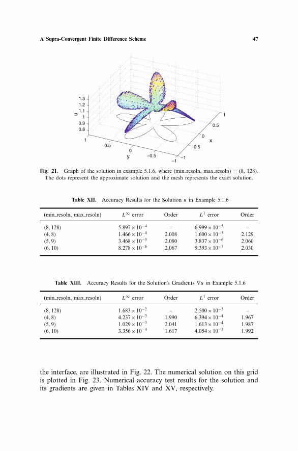
the interface, are illustrated in Fig. 20. The numerical solution on this gridis plotted in Fig. 21. Numerical accuracy test results for the solution andits gradients are given in Tables XII and XIII, respectively.

5.1.7. Example 7

Consider ∇ · (ρ∇u) = f on Ω = [−2,2] × [−2,2] with an exact solu-tion of u = cos(πx) sin(πy), where ρ = 2 + sin(πx) cos(πy). The interfaceis given by the set of points where φ =16y4 −x4 −32y2 +9x2 =0. A non-graded Cartesian grid with (min resoln, max resoln) = (8, 128), as well as


–1

–0.5

0

0.5

1

–1–0.5

00.5

1

0.80.9

11.11.21.3

x

y

u


Table XII. Accuracy Results for the Solution u in Example 5.1.6


(8,128) 5.897×10−4 – 6.999×10−5 –(4,8) 1.466×10−4 2.008 1.600×10−5 2.129(5,9) 3.468×10−5 2.080 3.837×10−6 2.060(6,10) 8.278×10−6 2.067 9.393×10−7 2.030

Table XIII. Accuracy Results for the Solution’s Gradients ∇u in Example 5.1.6


(8,128) 1.683×10−2 – 2.500×10−3 –(4,8) 4.237×10−3 1.990 6.394×10−4 1.967(5,9) 1.029×10−3 2.041 1.613×10−4 1.987(6,10) 3.356×10−4 1.617 4.054×10−5 1.992

the interface, are illustrated in Fig. 22. The numerical solution on this gridis plotted in Fig. 23. Numerical accuracy test results for the solution andits gradients are given in Tables XIV and XV, respectively.


Fig. 22. Domain Ω = [−2,2] × [−2,2] and the spatial discretization in examples 5.1.7and 5.2.5 with (min resoln, max resoln) = (8, 128).

–2–1.5

–1–0.5

00.5

11.5

2

–2–1.5

–1–0.5

00.5

11.5

2–1

–0.5

0

0.5

1

xy

u


5.1.8. Example 8

Consider a 3D Poisson equation ∇ · (ρ∇u)=f on Ω = [−0.75,0.75]×[−0.75,0.75] × [−0.75,0.75], with an exact solution of u= exp(−x2 − y2 −z2), where ρ =2+ sin(x +y +z). The interface is the surface of an ellipsoid


Table XIV. Accuracy Results for the Solution u in Example 5.1.7


(8,128) 3.876×10−2 – 4.420×10−3 –(4,8) 9.342×10−3 2.053 1.033×10−3 2.097(5,9) 2.262×10−3 2.046 2.473×10−4 2.062(6,10) 5.598×10−4 2.014 6.048×10−5 2.032

Table XV. Accuracy Results for the Solution’s Gradients ∇u in Example 5.1.7


(8,128) 2.803×10−1 – 8.066×10−2 –(4,8) 7.430×10−2 1.915 1.981×10−2 2.025(5,9) 1.975×10−2 1.911 4.896×10−3 2.017(6,10) 5.182×10−3 1.931 1.220×10−3 2.005

Table XVI. Accuracy Results for the Solution u in Example 5.1.8


(4,16) 2.413×10−4 – 9.603×10−5 –(8,32) 8.476×10−5 1.509 2.578×10−5 1.897(16,64) 2.370×10−5 1.838 7.602×10−6 1.762(32,128) 6.287×10−6 1.914 2.147×10−6 1.824

where φ = x2 + 9/4y2 + 4z2 − 0.25 = 0. A non-graded Cartesian grid with(min resoln, max resoln) = (4, 32), as well as the interface, are illustratedin Fig. 24. The numerical accuracy test results for the solution and its gra-dients are given in Tables XVI and XVII, respectively.

5.2. Heat Equation

We consider Eq. (2) in two and three spatial dimensions, where ρ is a(possibly different) constant on each subdomain. Again, we only computesolutions on Ω−. Dirichlet boundary conditions are applied on the inter-face. The time step in the Crank–Nicolson scheme is chosen as ∆t =∆x/2,where ∆x is the size of the smallest cell, so that an overall second-orderaccuracy is obtained. Since the solutions in the following examples decay


Fig. 24. Domain Ω = [−0.75,0.75] × [−0.75,0.75] × [−0.75,0.75] and the spatial discretiza-tion in example 5.1.8 with (min resoln, max resoln) = (4, 32).

Table XVII. Accuracy Results for the Solution’s Gradients ∇u in Example 5.1.8


(4,16) 1.229×10−2 – 2.969×10−3 –(8,32) 3.017×10−3 2.026 6.704×10−4 2.147(16,64) 9.018×10−4 1.742 1.694×10−4 1.985(32,128) 2.255×10−4 2.000 4.189×10−5 2.015

exponentially, we choose the final time as t =0.25, so that the solution atthe final time is not too small. Other choices of the final time would yieldsimilar results.

5.2.1. Example 1

Consider ut =∇ · (ρ∇u) on Ω = [−π,π ] × [−π,π ] with an exact solu-tion of u = e−2ρt sin(x) cos (y), where ρ = 1. The interface is given bythe set of points where φ =

√x2 + (y −1)2 − 1.5 = 0. Dirichlet boundary

condition is also applied on ∂Ω. An adaptive Cartesian grid with (minresoln, max resoln) = (8, 64), as well as the interface, are illustrated in



–2

0

2

–20

2

–0.5

0

0.5

xy

u


Fig. 25. The numerical solution at t = 0.25 on this grid is plotted in Fig.26. Numerical accuracy test results for the solution and its gradients aregiven in Tables XVIII and XIX, respectively.


Table XVIII. Accuracy Results for the Solution u in Example 5.2.1


(8,64) 1.073×10−2 – 2.278×10−3 –(16,128) 3.126×10−3 1.779 6.537×10−4 1.801(32,256) 7.847×10−4 1.994 1.675×10−4 1.965(64,512) 1.958×10−4 2.003 4.219×10−5 1.989

Table XIX. Accuracy Results for the Solution’s Gradients ∇u in Example 5.2.1


(8,64) 9.100×10−2 – 1.706×10−2 –(16,128) 2.837×10−2 1.682 4.713×10−3 1.856(32,256) 7.747×10−3 1.872 1.206×10−3 1.967(64,512) 1.983×10−3 1.966 3.036×10−4 1.990

5.2.2. Example 2

Consider ut = ∇ · (ρ∇u) on Ω = [−1,1] × [−1,1] with an exact solu-

tion of u=e−2π2 ρt cos(πx) cos(πy), where ρ =1. The interface is the sameas in example 5.1.4. The numerical solution at t = 0.25 on a grid with(min resoln, max resoln) = (8, 64) is plotted in Fig. 27. Numerical accu-racy test results for the solution and its gradients are given in Tables XXand XXI, respectively.

Table XX. Accuracy Results for the Solution u in Example 5.2.2


(8,64) 4.237×10−4 – 1.031×10−4 –(16,128) 1.229×10−4 1.786 2.696×10−5 1.935(32,256) 3.134×10−5 1.972 6.585×10−6 2.034(64,512) 7.872×10−6 1.993 1.616×10−6 2.026


–1–0.5

00.5

1

–0.5

0

0.5

1–4

–2

0

2

4

6

x 10–3

x

y

u


Table XXI. Accuracy Results for the Solution’s Gradients ∇u in Example 5.2.2


(8,64) 3.131×10−3 – 1.759×10−3 –(16,128) 9.487×10−4 1.722 5.142×10−4 1.775(32,256) 2.591×10−4 1.873 1.348×10−4 1.931(64,512) 6.919×10−5 1.905 3.428×10−5 1.976

5.2.3. Example 3

Consider ut = ∇ · (ρ∇u) on Ω = [−1,1] × [−1,1] with an exact solu-tion of u = e−2ρt cos(x) cos(y), where ρ = 1. The interface is the same asin example 5.1.5. The numerical solution at t =0.25 on a grid with (minresoln, max resoln) = (8, 64) is plotted in Fig. 28. Numerical accuracytest results for the solution and its gradients are given in Tables XXII andXXIII, respectively.

5.2.4. Example 4

Consider ut = ∇ · (ρ∇u) on Ω = [−1,1] × [−1,1] with an exact solu-tion of u = e−ρt (sin(x) + cos(y)), where ρ = 8. The interface is the sameas in example 5.1.6. The numerical solution at t = 0.25 on a grid with


–1–0.5

00.5

1

–0.5

0

0.5

1

0.5

0.52

0.54

0.56

0.58

0.6

x

y

u


Table XXII. Accuracy Results for the Solution u in Example 5.2.3


(8,64) 7.455×10−5 – 1.433×10−5 –(16,128) 1.871×10−5 1.994 3.501×10−6 2.034(32,256) 4.623×10−6 2.017 8.582×10−7 2.028(64,512) 1.148×10−6 2.009 2.122×10−7 2.016

Table XXIII. Accuracy Results for the Solution’s Gradients ∇u in Example 5.2.3


(8,64) 7.826×10−4 – 2.888×10−4 –(16,128) 2.307×10−4 1.762 7.475×10−5 1.950(32,256) 6.541×10−5 1.818 1.901×10−5 1.975(64,512) 1.824×10−5 1.842 4.785×10−6 1.991

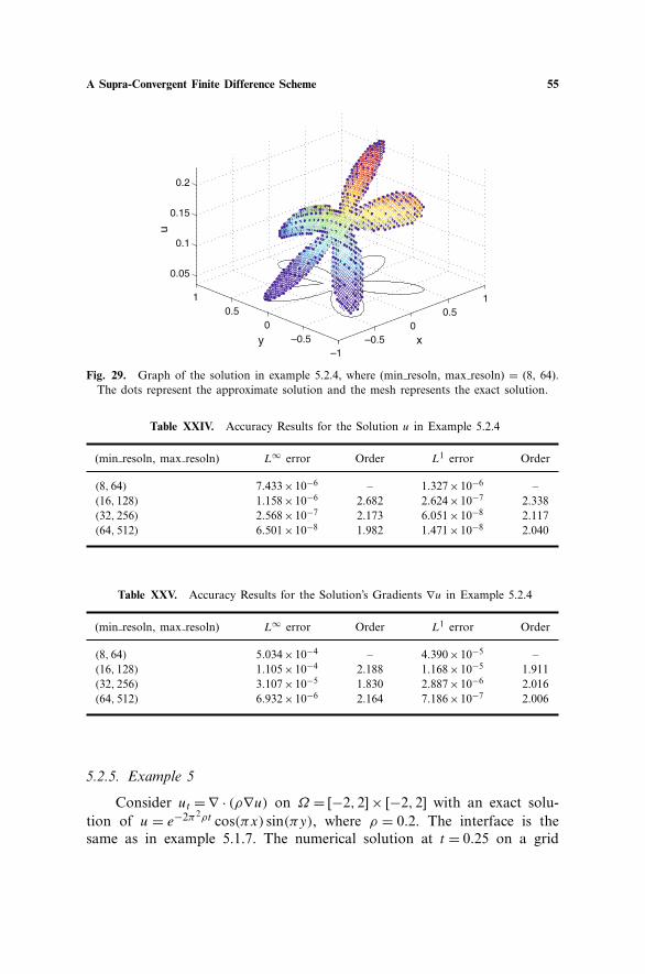
(min resoln, max resoln) = (8, 64) is plotted in Fig. 29. Numerical accu-racy test results for the solution and its gradients are given in TablesXXIV–XXVI, respectively.


–1–0.5

00.5

1

–0.50

0.51

0.05

0.1

0.15

0.2

xy

u


Table XXIV. Accuracy Results for the Solution u in Example 5.2.4


(8,64) 7.433×10−6 – 1.327×10−6 –(16,128) 1.158×10−6 2.682 2.624×10−7 2.338(32,256) 2.568×10−7 2.173 6.051×10−8 2.117(64,512) 6.501×10−8 1.982 1.471×10−8 2.040

Table XXV. Accuracy Results for the Solution’s Gradients ∇u in Example 5.2.4


(8,64) 5.034×10−4 – 4.390×10−5 –(16,128) 1.105×10−4 2.188 1.168×10−5 1.911(32,256) 3.107×10−5 1.830 2.887×10−6 2.016(64,512) 6.932×10−6 2.164 7.186×10−7 2.006

5.2.5. Example 5

Consider ut = ∇ · (ρ∇u) on Ω = [−2,2] × [−2,2] with an exact solu-tion of u = e−2π2ρt cos(πx) sin(πy), where ρ = 0.2. The interface is thesame as in example 5.1.7. The numerical solution at t = 0.25 on a grid


–2–1.5

–1–0.5

00.5

11.5

2

–2

–1

0

1

2

–0.2

0

0.2

x

y

u


Table XXVI. Accuracy Results for the Solution’s Gradients ∇u in Example 5.2.4


(8,64) 5.034×10−4 – 4.390×10−5 –(16,128) 1.105×10−4 2.188 1.168×10−5 1.911(32,256) 3.107×10−5 1.830 2.887×10−6 2.016(64,512) 6.932×10−6 2.164 7.186×10−7 2.006

Table XXVII. Accuracy Results for the Solution u in Example 5.2.5


(8,64) 1.741×10−2 – 3.872×10−3 –(16,128) 4.111×10−3 2.083 8.922×10−4 2.118(32,256) 1.011×10−3 2.024 2.158×10−4 2.048(64,512) 2.519×10−4 2.005 5.304×10−5 2.024

with (min resoln, max resoln) = (8, 64) is plotted in Fig. 30. Numericalaccuracy test results for the solution and its gradients are given in TablesXXVII and XXVIII, respectively.


Table XXVIII. Accuracy Results for the Solution’s Gradients ∇u in Example 5.2.5


(8,64) 1.155×10−1 – 4.272×10−2 –(16,128) 3.102×10−2 1.896 1.073×10−2 1.994(32,256) 8.436×10−3 1.878 2.671×10−3 2.006(64,512) 2.283×10−3 1.886 6.670×10−4 2.002

Fig. 31. Domain Ω = [−0.75,0.75] × [−0.75,0.75] × [−0.75,0.75] and the spatial discretiza-tion in example 5.2.6 with (min resoln, max resoln) = (4, 32).

5.2.6. Example 6

Consider a 3D heat equation ut = ∇ · (ρ∇u) on Ω = [−0.75,0.75] ×[−0.75,0.75] × [−0.75,0.75] with an exact solution of u = e−t (sin(x) +cos(y) + cos(z). The interface is the surface of a sphere on whichφ =

√x2 +y2 + z2 − 0.7. A non-graded Cartesian grid with (min resoln,

max resoln) = (4, 32), as well as the interface, are illustrated in Fig. 31.Numerical accuracy test results for the solution and its gradients are givenin Tables XXIX and XXX, respectively.


Table XXIX. Accuracy Results for the Solution u in Example 5.2.6


(4,16) 6.239×10−4 – 1.537×10−4 –(8,32) 1.473×10−4 2.083 3.640×10−5 2.079(16,64) 3.912×10−5 1.913 8.779×10−6 2.052(32,128) 1.008×10−5 1.956 2.144×10−6 2.034

Table XXX. Accuracy Results for the Solution’s Gradients ∇u in Example 5.2.6


(4,16) 6.950×10−3 – 2.952×10−3 –(8,32) 1.876×10−3 1.889 7.901×10−4 1.902(16,64) 5.262×10−4 1.834 2.027×10−4 1.962(32,128) 1.390×10−4 1.920 5.145×10−5 1.979

6. CONCLUSIONS

We have proposed finite difference algorithms for the variable coeffi-cient Poisson equation as well as for the heat equation on irregulardomains and non-graded Cartesian grids. These schemes leverage bothadaptivity strategy and the quadratic treatment of the Dirichlet bound-ary condition near the interface and produce second-order accuracy forthe solution and its gradients. T-junction nodes neighboring the irregu-lar interface are excluded by imposing that cells on the interface havethe finest resolution. Sampling the solution at the nodes produces efficientand simple procedures that can be applied in a dimension-by-dimensionframework. At T-junctions, linear interpolations are used to generate inter-mediate ghost values used in the discretizations. These intermediate val-ues introduce spurious O(1) errors that are successfully removed by linearcombinations of the discretizations in the transversal directions. For nodesneighboring the interface, a quadratic fitting of the signed distance levelset function is used to find the location of the interface, and the Dirich-let boundary value is obtained either explicitly when a analytic formulais known or by quadratic interpolation of the neighboring nodal values.The calculation of the solution’s gradients involves the same cells as thoseused in the discretization of the Poisson or heat equation, hence preservingthe locality and ease of implementation of the method. We have presented


ample numerical results to demonstrate the second-order accuracy in theL1 and L∞ norms for the solution and its gradients.

ACKNOWLEDGMENTS

The research of F. Gibou was supported in part by the Alfred P.Sloan Foundation through a research fellowship in Mathematics.

REFERENCES

1. Aftosmis, M. J., Berger, M. J., and Melton, J. E. (1998). Adaptive Cartesian mesh gener-ation. In CRC Handbook of Mesh Generation (Contributed Chapter).

2. Almgren, A. (1991). A Fast Adaptive Vortex Method Using Local Corrections. PhD the-sis, University of California, Berkeley.

3. Almgren, A., Bell, J., Colella, P., Howell, L., and Welcome, M. (1998). A conservativeadaptive projection method for the variable density incompressible navier-stokes equa-tions. J. Comput. Phys. 142, 1–46.

4. Almgren, A., Buttke, R., and Colella, P. (1994). A fast adaptive vortex method in threedimensions. J. Comput. Phys. 113, 177–200.

5. Berger, M., and Oliger, J. (1984). Adaptive mesh refinement for hyperbolic partial differ-ential equations. J. Comput. Phys. 53, 484–512.

6. Chen, S., Merriman, B., Osher, S., and Smereka, P. (1997). A simple level set method forsolving Stefan problems. J. Comput. Phys. 135, 8–29.

7. Babuska, I., Flaherty, J. E., Henshaw, W. D., Hopcroft, J. E., Oliger, J. E., and Tezduyar,T. (eds.) (1995). Modeling, Mesh Generation, and Adaptive Numerical Methods for PartialDifferential Equations. Springer Verlag, Berlin, 450 pp.

8. Fedkiw, R., Aslam, T., Merriman, B., and Osher, S. (1999). A non-oscillatory Eulerianapproach to interfaces in multimaterial flows (the ghost fluid method). J. Comput. Phys.152, 457–492.

9. Gibou, F., and Fedkiw, R. (2005). A fourth order accurate discretization for the laplaceand heat equations on arbitrary domains, with applications to the stefan problem.J, Comput. Phys. 202, 577–601.

10. Gibou, F., Fedkiw, R., Caflisch, R., and Osher, S. (2003). A level set approach for thenumerical simulation of dendritic growth. J. Sci. Comput. 19, 183–199.

11. Gibou, F., Fedkiw, R., Cheng, L.-T., and Kang, M. (2002). A second–order–accuratesymmetric discretization of the poisson equation on irregular domains. J. Comput. Phys.176, 205–227.

12. Johansen, H., and Colella, P. (1998). A cartesian grid embedded boundary method forpoisson’s equation on irregular domains. J. Comput. Phys. 147, 60–85.

13. Johnson, C. (1987). Numerical Solution of Partial Differential Equations by the Finite Ele-ment Method. Cambridge University Press, New York, NY.

14. Jomaa, Z., and Macaskill, C. (2005). The embedded finite difference method for thepoisson equation in a domain with an irregular boundary and dirichlet boundary condi-tions. J. Comput. Phys. 202, 488–506.

15. Kreiss, H. O., Manteuffel, H.-O., Schwartz, T. A., Wendroff, B., and White, A. B., Jr.(1986). Supra-convergent schemes on irregular grids. Math. Comp. 47, 537–554.

16. LeVeque, R., and Li, Z. (1994). The immersed interface method for elliptic equations withdiscontinuous coefficients and singular sources. SIAM J. Numer. Anal. 31, 1019–1044.


17. Lipnikov, K., Morel, J., and Shashkov, M. (2004). Mimetic finite difference methodsfor diffusion equations on non-orthogonal non-conformal meshes. J. Comput. Phys. 199,589–597.

18. Liu, X., Fedkiw, R., and Kang, M. (2000). A boundary condition capturing method forPoisson’s equation on irregular domains. J. Comput. Phys. 154, 151.

19. Losasso, F., Fedkiw, R., and Osher, S. (2006). Spatially adaptive techniques for level setmethods and incompressible flow. Comput. Fluids 35, 995–1010.

20. Losasso, F., Gibou, F., and Fedkiw, R. (2004). Simulating water and smoke with anoctree data structure. SIGGRAPH 2004, ACM TOG 23, 457–462.

21. Manteuffel, T., and White, A. (1986). The numerical solution of second-order boundaryvalue problems on nonuniform meshes. Math. Comput. 47(176), 511–535.

22. Mayo, A. (1984). The fast solution of poisson’s and the biharmonic equations on irregu-lar regions. SIAM J. Numer. Anal. 21, 285–299.

23. McCorquodale, P., Colella, P., Grote, D., and Vay, J.-L. (2004). A node-centered localrefinement algorithm for poisson’s equation in complex geometries. J. Comput. Phys. 201,34–60.

24. McKenney, A., and Greengard, L. (1995). A fast poisson solver for complex geometries.J. Comput. Phys. 118, 348–355.

25. Min, C., Gibou, F., and Ceniceros, H. D. (2006). A supra-convergent finite differencescheme for the variable coefficient poisson equation on non-graded grids. J. Comput.Phys. 218(1), 123–140.

26. Peskin, C. (1977). Numerical analysis of blood flow in the heart. J. Comput. Phys. 25,220–252.

27. Popinet, S. (2003). Gerris: a tree-based adaptive solver for the incompressible euler equa-tions in complex geometries. J. Comput. Phys. 190, 572–600.

28. Saad, Y. (1996). Iterative Methods for Sparse Linear Systems. PWS Publishing, NewYork, NY.

29. Samet, H. (1989). The Design and Analysis of Spatial Data Structures. Addison-Wesley,New York.

30. Samet, H. (1990). Applications of Spatial Data Structures: Computer Graphics, ImageProcessing and GIS. Addison-Wesley, New York.

31. Schmidt, A. (1996). Computation of three dimensional dendrites with finite elements.J. Comput. Phys. 125, 293–312.

32. Shortley, G. H., and Weller, R. (1938). The numerical solution of laplace’s equation.J. Appl. Phys. 9, 334–348.

33. Strain, J. (1999). Tree methods for moving interfaces. J. Comput. Phys. 151, 616–648.34. Verfurth, R. (1996). A Review of a Posteriori Error Estimation and Adaptive Mesh-Refine-

ment Techniques. Wiley-Teubner, Berlin.35. Young, D., Melvin, R., Bieterman, M., Johnson, F., Samant, S., and Bussoletti, J. (1991).

A locally refined rectangular grid finite element method: application to computationalfluid dynamics and computational physics. J. Comput. Phys. 92, 1–66.

a supra-convergent finite difference scheme for the...

Documents