a supporting infrastructure for wireless sensor networks ... · a supporting infrastructure for...
TRANSCRIPT

Thanh-Dien Tran
A Supporting Infrastructure for Wireless Sensor Networks
in Critical Industrial Environments
Thesis submitted as partial fulfillment of the requirements of the Doctoral Program on Information Science and Technology in the University of Coimbra, for the award of Doctor in the domain of Telematics Networking and Communications under the supervision of Professor Doctor Jorge Miguel Sá Silva.
Coimbra 2013


UNIVERSITY OF COIMBRA
FACULTY OF SCIENCES AND TECHNOLOGY
Department of Informatics Engineering
A Supporting Infrastructure for Wireless Sensor Networks in
Critical Industrial Environments
Thanh-Dien Tran
Coimbra
2013

The whole of science is nothing more than a refinement of everyday thinking.
Albert Einstein

i
Acknowledgements
I am especially grateful to my supervisor, Dr. Jorge Miguel Sá Silva, and I would like to
thank him for inspiring me in this exciting research area and giving me advice whenever
I needed it. I am grateful for his constant encouragement, support, and guidance during
my PhD at the University of Coimbra. I would also give my special thanks to Dr. Luiz
Henrique Andrade Correia at Federal University of Lavras – UFLA for his ideas and
cooperative works during his time in the University of Coimbra.
I wish to thank to Dr. Carlos Pina Teixeira, the CEO of Eneida company, who gave me
the opportunity not only to do research in the Wireless Solutions Group of Eneida, but
also to support the funding. I would also like to thank Mr. João Marco Lopes, Eneida
Business Manager, who has provided me with necessary assistance and support.
I am very grateful to have had the opportunity to work with so many wonderful people at
the wireless Solutions Group, Eneida and the Laboratory of Telematics and
Communication of Informatics Engineering of the University of Coimbra, Portugal. A
special thank to José Oliveira, Engineering & Development Manager, and Nuno Sousa
at Eneida. I would like to thank my colleagues of the sensor network group, in particular,
Ricardo Silva, David Nunes, Duarte Raposo, André Gomes, Vasco Pereira, and André
Rodrigues.
I would like to express my gratitude to Ms. Diana Taborda, the manager of postgraduate
programs of DEI, University of Coimbra, for her instantaneous responsiveness and
outstanding helps. Especially, I would like to thank her for the time and effort taken to
review this thesis and give me useful advices to improve it.
This work was sponsored by the Portuguese Ministry of Science (scholarship contract
SFRH/BDE/51738/2011), and partially supported by the Project QREN PULSE
(Scholarship contract CB/C17/2010/01), TRIG Program of Can Tho University -
Vietnam, GINSENG Project (under grant agreement n° 224282), and the Eneida
Company.
To my parents and brothers for their constant encouragement and understanding when I
could not come home for such a long time. I would like to express my gratitude to my
wife, Ngoc Diem, and my daughter, Ngoc Minh, for their love, who fully supported me
and stood by me. Especially, I would like to express my deepest gratitude to my wife for
being pregnant and bringing a wonderful child into the world during the time I was
working on my thesis far away.
Without the help of the particular people mentioned above, I would have faced many
difficulties while writing this doctoral thesis.
ii
Resumo
As Redes de Sensores Sem Fios (RSSFs) têm uma aplicabilidade muito elevada nas
mais diversas áreas, como na indústria, nos sistemas militares, na saúde e nas casas
inteligentes. No entanto, continuam a existir várias limitações que impedem que esta
tecnologia tenha uma utilização extensiva. A fiabilidade é uma destas principais
limitações que tem atrasado a adopção das RSSFs em ambientes industriais,
principalmente quando sujeitos a elevadas interferências e ruídos. Por outro lado, a
interoperabilidade é também um dos principais requisitos a cumprir nomeadamente com
o avanço para o paradigma da Internet of Things.
A determinação da localização dos nós, principalmente dos nós móveis, é, também ele,
um requisito crítico em muitas aplicações. Esta tese de doutoramento propõe novas
soluções para a integração e para a localização de RSSFs que operem em ambientes
industriais e críticos.
Como os nós sensores são, na maioria das vezes, instalados e deixados sem
intervenção humana durante longos períodos de tempo, isto é, meses ou mesmo anos,
é muito importante oferecer processos de comunicação fiável. No entanto, muitos
problemas ocorrem durante a transmissão dos pacotes, nomeadamente devido a
ruídos, interferências e perda de potência do sinal. A razão das interferências deve-se à
existência de mais do que uma rede ou ao espalhamento espectral que ocorre em
determinadas frequências. Este tipo de problemas é mais severo em ambientes
dinâmicos nos quais novas fontes de ruído pode ser introduzidas em qualquer instante
de tempo, nomeadamente com a chegadas de novos dispositivos ao meio.
Consequentemente, é necessário que as RSSFs tenham a capacidade de lidar com as
limitações e as falhas nos processos de comunicação. O protocolo Dynamic MAC
(DunMAC) proposto nesta dissertação utiliza técnicas de rádio cognitivo (CR) para que
a RSSF se adapte, de forma dinâmica, a ambientes instáveis e ruidosos através da
selecção automática do melhor canal durante o período de operação.
As RSSFs não podem operar em isolação completa do meio, e necessitam de ser
monitoradas e controladas por aplicações externas. Apesar de ser possível adicionar a
pilha protocolar IP aos nós sensores, este procedimento não é adequado para muitas
aplicações. Para estes casos, os modelos baseados em gateway ou proxies continuam
a apresentar-se preferíveis para o processo de integração. Um dos desafios existentes
para estes processos de integração é a sua adaptabilidade, isto é, a capacidade da
gateway ou do proxy poder ser reutilizado sem alterações por outras aplicações. A

iii
razão desta limitação deve-se aos consumidores finais dos dados serem aplicações e
não seres humanos. Logo, é difícil ou mesmo impossível criar normas para as
estruturas de dados dada a infinidade de diferentes formatos. É então desejável
encontrar uma solução que permita uma integração transparente de diferentes RSSFs e
aplicações. A linguagem Sensor Traffic Description Language (STDL) proposta nesta
dissertação propõe uma solução para esta integração através de gateways e proxies
flexíveis e adaptados à diversidade de aplicações, e sem recorrer à reprogramação.
O conhecimento da posição dos nós sensores é, também ele, crítico em muitas
aplicações industriais como no controlo da deslocação dos objectos ou trabalhadores.
Para além do mais, a maioria dos valores recolhidos dos sensores só são úteis quando
acompanhados pelo conhecimento do local onde esses valores foram recolhidos. O
Global Positioning Systems (GPS) é a mais conhecida solução para a determinação da
localização. No entanto, o recurso ao GPS em cada nó sensor continua a ser
energeticamente ineficiente e impraticável devido aos custos associados. Para além
disso, os sistemas GPS não são apropriados para ambientes in-door.
Este trabalho de doutoramento propõe-se actuar nestas áreas. Em particular, é
proposto, implementado e avaliado o protocolo DynMAC para oferecer fiabilidade às
RSSFs. Para a segunda temática, a linguagem STDL e o seu motor são propostos para
suportar a integração de ambientes heterogéneos de RSSFs e aplicações. As soluções
propostas não requerem reprogramação e suportam também serviços de localização
nas RSSFs. Diferentes métodos de localização foram avaliados para estimar a
localização dos nós. Assim, com estes métodos as RSSFs podem ser usadas como
componentes para integrar e suportar a Futura Internet.
Todas as soluções propostas nesta tese foram implementadas e validadas tanto em
simulação com em plataformas práticas, laboratoriais e industriais.

iv
Abstract
The Wireless Sensor Network (WSN) has a countless number of applications in almost
all of the fields including military, industrial, healthcare, and smart home environments.
However, there are several problems that prevent the widespread of sensor networks in
real situations. Among them, the reliability of communication especially in noisy
industrial environments is difficult to guarantee. In addition, interoperability between the
sensor networks and external applications is also a challenge. Moreover, determining
the position of nodes, particularly mobile nodes, is a critical requirement in many types
of applications. My original contributions in this thesis include reliable communication,
integration, localization solutions for WSNs operating in industrial and critical
environments.
Because sensor nodes are usually deployed and kept unattended without human
intervention for a long duration, e.g. months or even years, it is a crucial requirement to
provide the reliable communication for the WSNs. However, many problems arise during
packet transmission and are related to the transmission medium (e.g. signal path-loss,
noise and interference). Interference happens due to the existence of more than one
network or by the spectral spread that happens in some frequencies. This type of
problem is more severe in dynamic environments in which noise sources can be
introduced at any time or new networks and devices that interfere with the existing one
may be added. Consequently, it is necessary for the WSNs to have the ability to deal
with the communication failures. The Dynamic MAC (DynMAC) protocol proposed in
this thesis employs the Cognitive Radio (CR) techniques to allow the WSNs to adapt to
the dynamic noisy environments by automatically selecting the best channel during its
operation time.
The WSN usually cannot operate in complete isolation, but it needs to be monitored,
controlled and visualized by external applications. Although it is possible to add an IP
protocol stack to sensor nodes, this approach is not appropriate for many types of
WSNs. Consequently, the proxy and gateway approach is still a preferred method for
integrating sensor networks with external networks and applications. The problem of the
current integration solutions for WSNs is the adaptability, i.e., the ability of the gateway
or proxy developed for one sensor network to be reused, unchanged, for others which
have different types of applications and data frames. One reason behind this problem is
that it is difficult or even impossible to create a standard for the structure of data inside
the frame because there are such a huge number of possible formats. Consequently, it

v
is necessary to have an adaptable solution for easily and transparently integrating
WSNs and application environments. In this thesis, the Sensor Traffic Description
Language (STDL) was proposed for describing the structure of the sensor networks’
data frames, allowing the framework to be adapted to a diversity of protocols and
applications without reprogramming.
The positions of sensor nodes are critical in many types of industrial applications such
as object tracking, location-aware services, worker or patient tracking, etc. In addition,
the sensed data is meaningless without the knowledge of where it is obtained. Perhaps
the most well-known location-sensing system is the Global Positioning System (GPS).
However, equipping GPS sensor for each sensor node is inefficient or unfeasible for
most of the cases because of its energy consumption and cost. In addition, GPS is not
appropriate in some environments, e.g., indoors. Similar to the original concept of
WSNs, the localization solution should also be cheap and with low power consumption.
This thesis aims to deal with the above problems. In particular, in order to add the
reliability for WSN, DynMAC protocol was proposed, implemented and evaluated. This
protocol adds a mechanism to automatically deal with the noisy and changeable
environments. For the second problem, the STDL and its engine provide the adaptable
capability to the framework for interoperation between sensor networks and external
applications. The proposed framework requires no reprogramming when deploying it for
new applications and protocols of WSNs. Moreover, the framework also supports
localization services for positioning the unknown position sensor nodes in WSNs. The
different localization methods are employed to estimate the location of mobile nodes.
With the proposed framework, WSNs can be used as plug and play components for
integrating with the Future Internet. All the proposed solutions were implemented and
validated using simulation and real testbeds in both the laboratory and industrial
environments.

vi
Foreword
The work in this thesis was conducted at the Laboratory of Telematics and
Communication of the Centre for Informatics and Systems of the University of Coimbra
and the Eneida Company within the context of the BDE scholarship number:
SFRH/BDE/51738/2011:
The works done in this thesis resulted in the following publications:
T.D. Tran, D. Nunes, C. Herrera, and J. Sá Silva, “An Adaptable Framework for
Interoperating Between Wireless Sensor Networks and external Applications,” 3rd
International Conference on Sensor Networks (SENSORNETS 2014), Lisbon,
2014.
T.D. Tran, D. Nunes, A. Gomes, and J. Sá Silva, “An Adaptive Model for
Exposing WSN as a Service platform,” In Procedding of 4th National
Symposium on Informatics (iNForum 2012), Caparica , Lisbon, 2012.
D. Nunes, T.D. Tran, D. Raposo, A. Pinto, A. Gomes, and J. Sá Silva, “A Web
Service-Based Framework Model for People-Centric Sensing Applications
Applied to Social Networking,” Sensors, vol. 12, no, 2, pp. 1688-1701, February
2012.
T.D. Tran, R. Silva, D. Nunes, and J. Sá Silva, “Characteristics of Channels of
IEEE 802.15.4 Compliant Sensor Networks,” Wireless Personal
Communications, vol. 67, no. 3, pp. 541-556, December 2011.
T. D. Tran, R. Silva, D. Nunes, and J. Sá Silva, “Channel Quality of IEEE
802.15.4 based sensor networks,” In Procedding of 10ª Conferência sobre
Redes de Computadores (CRC 2010), Braga, Portugal, 2010.
T.D. Tran and J. Sá Silva, “A Framework for Integrating WSNs and external
environments,” in proceeding of 5th IFAC International Conference on
Management Control and Production and Logistics (MCPL 2010), Coimbra,
Portugal, September 8-10, 2010.

vii
F. Cheng, T.D. Tran, S. Roschke, and Ch. Meinel, “A Specialized Tool for
Simulating Lock-Keeper Data Transfer,” in Proceedings of 24th IEEE
International Conference on Advanced Information Networking and Applications
(AINA'10), IEEE Press, Perth, Australia, April 20-23, 2010.
S. Roschke, F. Cheng, T.D. Tran, and Ch. Meinel, “A Theoretical Model of Lock-
Keeper Data Exchange and its Practical Verification,” in Proceedings of 6th IFIP
International Conference on Network and Parallel Computing (NPC'09), IEEE
Press, Gold Coast, Australia, October 19 - 21, 2009
T.D. Tran, J. Oliveira, J. Sá Silva, V. Pereira, N. Sousa, D. Raposo, and F.
Cardoso, “A Scalable Localization System for Critical Controlled Wireless Sensor
Networks,” the Industrial Electronics Magazine, 2013 (Submitted).
L. H. A. Correia, T.D. Tran, V. Pereira, J. C. Giacomin, and J. Sá Silva,
“DynMAC: a resistant MAC protocol to coexistence in wireless sensor networks,”
Computer Networks, 2013 (Submitted).
T.D Tran and J. Sá Silva, “A Supporting Infrastructure for Wireless Sensor
Networks in Critical and Industrial Environments,” Mobile Networks and
Applications, 2013 (Submitted).

viii
Table of Content
ACKNOWLEDGEMENTS ........................................................................................................... I
RESUMO ...................................................................................................................................... II
ABSTRACT ................................................................................................................................. IV
FOREWORD ............................................................................................................................... VI
LIST OF FIGURES ................................................................................................................. XIV
LIST OF TABLES ................................................................................................................... XVI
LIST OF ACRONYMS .......................................................................................................... XVII
1 INTRODUCTION ................................................................................................................ 1
1.1 Motivation and problem Statement ....................................................................................... 1
1.1.1 Reliable Communication .................................................................................................... 2
1.1.2 Integration .......................................................................................................................... 3
1.1.3 Localization ........................................................................................................................ 5
1.2 Objectives ................................................................................................................................ 7
1.3 Contributions ........................................................................................................................... 8
1.4 Outline of the Thesis ............................................................................................................... 9
2 LITERATURE REVIEW .................................................................................................. 10
2.1 Overview ................................................................................................................................. 11
2.1.1 Wireless Sensor Networks ............................................................................................... 11
2.1.2 Challenges ....................................................................................................................... 12
2.1.3 Requirements ................................................................................................................... 14
2.1.4 Supporting Services ......................................................................................................... 15

ix
2.2 Medium Access Control protocol (MAC) for WSNs ........................................................... 16
2.2.1 Contention-based MAC Protocols ............................................................................... 18
2.2.1.1 Asynchronous Coordination Contention-based MAC Protocols .......................... 18
2.2.1.2 Synchronous Coordination Contention-based MAC Protocols ............................ 21
2.2.2 Schedule-based MAC Protocols.................................................................................. 22
2.2.2.1 Scheduling of Communication Link ...................................................................... 22
2.2.2.2 Scheduling of Transmitters .................................................................................. 25
2.2.2.3 Scheduling of Receivers ...................................................................................... 26
2.2.3 Hybrid MAC Protocols ................................................................................................. 27
2.3 Wireless network Coexistence and Cognitive Radio (CR) ................................................ 28
2.3.1 Wireless Network Coexistence ........................................................................................ 28
2.3.2 Cognitive Radio (CR) ....................................................................................................... 31
2.4 Integrating Sensor networks With External Environments .............................................. 32
2.4.1 Internetworking ................................................................................................................ 32
2.4.1.1 Gateway-based Approach ........................................................................................ 33
2.4.1.1.1 Application-level Gateway ................................................................................. 33
2.4.1.1.2 Low-level Gateway ............................................................................................ 33
2.4.1.2 IP-enabled WSNs ..................................................................................................... 35
2.4.2 Integration ........................................................................................................................ 36
2.4.2.1 Direct Access Approach ........................................................................................... 36
2.4.2.2 Indirect Access Approach ......................................................................................... 38
2.4.3 Comparison of the Integration Methods for WSNS ......................................................... 39
2.5 Localization ............................................................................................................................ 42
2.5.1 Measurement Techniques ............................................................................................... 42
2.5.1.1 Received Signal Strength Indication (RSSI) ............................................................. 43
2.5.1.2 Propagation Time ..................................................................................................... 43
2.5.1.3 Angle of Arrival ......................................................................................................... 44
2.5.2. Localization Methods ...................................................................................................... 45
2.5.2.1 Localization Methods for Ad-hoc Sensor Networks.................................................. 46

x
2.5.2.1.1 Lateration-based Methods ................................................................................. 47
2.5.2.1.2 Point-In-Triangle Test ........................................................................................ 50
2.5.2.1.3 Multidimensional Scaling (MDS)-based Methods ............................................. 51
2.5.2.1.4 Mass-spring based Optimization ....................................................................... 52
2.5.2.1.5 Sequential Quadratic Programming .................................................................. 52
2.5.2.1.6 Simulated Annealing Localization ..................................................................... 53
2.5.2.1.7 Support Vector Machine .................................................................................... 54
2.5.2.1.8 Hybrid Methods ................................................................................................. 54
2.5.2.2 Localization Methods for Controlled Sensor Networks ............................................. 55
2.5.2.2.1 Proximity ............................................................................................................ 55
2.5.2.2.2 Centroid Method ................................................................................................ 56
2.5.2.2.3 Lateration ........................................................................................................... 56
2.5.2.2.4 Angulation .......................................................................................................... 57
2.5.2.2.5 Kalman filter....................................................................................................... 58
2.5.2.2.6 Pattern Matching-based methods ..................................................................... 60
2.6 Some Related Projects.......................................................................................................... 64
2.7 Summary ................................................................................................................................ 65
3 QUALITY OF CHANNELS OF IEEE 802.15.4 COMPLIANT SENSOR
NETWORKS AND DYNAMIC MAC....................................................................................... 66
3.1 Introduction ............................................................................................................................ 67
3.2 An Empirical Study of Quality of Channels of IEEE 802.15.4 Compliant Sensor
Networks....................................................................................................................................... 68
3.2.1 IEEE 802.15.4 Standard .................................................................................................. 68
3.2.2 Related Work ................................................................................................................... 70
3.2.3 Experimental Environments ............................................................................................. 71
3.2.4 Study Method ................................................................................................................... 72
3.2.5 Experimental Results ....................................................................................................... 74
3.2.5.1 The Characteristics of Channels in Clean Environments ......................................... 74
3.2.5.2 Effects of Interference on IEEE 802.15.4 based Sensor Networks. ......................... 77

xi
3.2.5.3 IEEE 802.15.4 Channel Quality in Noisy Environment ............................................ 78
3.2.5.4 Characteristics of Channels of IEEE 802.15.4 in Multi-motes Sensor Network ....... 79
3.2.6 Discussion ........................................................................................................................ 80
3.3 Dynamic Medium Access Control protocol (DynMAC) ..................................................... 81
3.3.1 Context ............................................................................................................................. 81
3.3.2 Related Work ................................................................................................................... 82
3.3.3 Ginseng MAC protocol (GinMAC) .................................................................................... 85
3.3.3.1 Topology Control Mechanism ................................................................................... 86
3.3.3.2 GinMAC Slot Allocation ............................................................................................ 86
3.3.4 Dynamic Channel Allocation MAC Protocol for WSN (DynMAC) .................................... 88
3.3.4.1 Network Synchronization .......................................................................................... 89
3.3.4.1.1 Local Best Channel Selection ........................................................................... 90
3.3.4.1.2 Network Joining ................................................................................................. 92
3.3.4.2 Global Best Channel Selection ................................................................................. 93
3.3.4.3 Periodically Re-evaluating the Best Channel ........................................................... 96
3.3.4.4 Recovery from Connection Loss .............................................................................. 96
3.3.5 Experiments and Results ................................................................................................. 97
3.3.5.1 Experiments with Simulation .................................................................................... 97
3.3.5.1.1 Scanning and Network Coverage Time ............................................................ 98
3.3.5.1.2 Handoff Time ..................................................................................................... 99
3.3.5.2 Experiments With Testbed ...................................................................................... 99
3.3.5.2.1 Evaluation of the Quality of Different Channels .............................................. 100
3.3.5.2.2 Scanning and Network Coverage Time .......................................................... 102
3.3.5.2.3 Dynamic Noise and Interference Detection .................................................... 104
3.3.5.2.4 Recovery from Connection Loss ..................................................................... 105
3.4 Summary .............................................................................................................................. 105
4 THE INTEGRATION FRAMEWORK AND SENSOR TRAFFIC DESCRIPTION
LANGUAGE (STDL) ................................................................................................................ 106
4.1 Introduction ......................................................................................................................... 107

xii
4.2 The Interoperability Model .................................................................................................. 110
4.2.1 The Gateway .................................................................................................................. 111
4.2.2 The proxy ....................................................................................................................... 113
4.3 Sensor Traffic Description Language (STDL) .................................................................. 115
4.3.1 Overview of the Language ............................................................................................. 115
4.3.2 The General Content Model of STDL ............................................................................ 118
4.3.3 The Frame Identification ................................................................................................ 119
4.3.4 The Frame Header Specification ................................................................................... 121
4.3.5 The Frame Content Specification .................................................................................. 124
4.3.5.1 The Field Type ........................................................................................................ 124
4.3.5.2 Simple Frame Description ...................................................................................... 125
4.3.5.3 Data Table Frame Description ................................................................................ 126
4.3.5.4 Complex Frame Description ................................................................................... 127
4.3.6 STDL Editor .................................................................................................................... 130
4.4 The STDL engine ................................................................................................................. 131
4.5 Prototype and Example Applications ................................................................................ 135
4.5.1 Prototype ........................................................................................................................ 135
4.5.2 Example Applications ..................................................................................................... 135
4.6 Conclusion ........................................................................................................................... 138
5 LOCALIZATION SYSTEM FOR WIRELESS SENSOR NETWORKS ................... 139
5.1 Introduction .......................................................................................................................... 140
5.2 Related Work ........................................................................................................................ 141
5.3 The Application Scenarios ................................................................................................. 147
5.4 Scalable Localization System ............................................................................................ 149
5.4.1 General Model of the System ........................................................................................ 149
5.4.2 Localization Middleware ................................................................................................. 150
5.4.3 Localization Methods ..................................................................................................... 151

xiii
5.4.4 Scalable Mechanisms .................................................................................................... 152
5.5 The Testbeds ....................................................................................................................... 155
5.5.1 Sensor Platform ............................................................................................................. 155
5.5.2 Testbed Environments ................................................................................................... 156
5.6 Experimental Results .......................................................................................................... 157
5.6.1 RSSI Calibration ............................................................................................................ 158
5.6.2 The Spread and Distribution of RSSI Values ................................................................. 160
5.5.3 Training Dataset ............................................................................................................. 161
5.6.4 Evaluating the Lateration Localization Methods ............................................................ 161
5.6.5 Evaluating the Localization Methods with the Laboratory Testbed ............................... 162
5.6.6 Evaluating the Localization Methods with the Testbed in industrial Environment ......... 163
5.7 Summary .............................................................................................................................. 166
6 CONCLUSION AND FUTURE WORK ........................................................................ 167
6.1 Conclusion ........................................................................................................................... 168
6.2 Future Work ......................................................................................................................... 170
REFERENCES .......................................................................................................................... 171
APPENDIX A: STDL GRAMMAR .................................................................................... 190
A.1 The syntax of the STDL in Extended Backus-Naur Form (EBNF) ................................. 190
A.2 The syntax graphs of the STDL. ........................................................................................ 192

xiv
List of Figures
Fig. 2.1 A Category for MAC Protocols for WSNs ......................................................... 18
Fig. 2.2 Comparison of timelines between LPL’s extended preamble and X-MAC’s
short preamble approach [62] ............................................................................... 20
Fig. 2.3 Category of Localization Methods .................................................................... 46
Fig. 2.4 Circle Lateration Localization Technique ......................................................... 48
Fig. 2.5 Hyperbolic Lateration Localization Technique ................................................. 57
Fig. 2.6 Angulation Localization Method ....................................................................... 58
Fig. 2.7 Kalman Filter Algorithm.................................................................................... 60
Fig. 2.8 An Example of a Neural Network with 3 Layers (4 input neurons, 6 hidden
neurons, 3 output neurons) ................................................................................... 63
Fig. 3.1 Interference Between IEEE 802.15.4 and IEEE 802.11g ................................. 69
Fig. 3.2 The Workflow of the Nodes in the Experimental Network ................................. 73
Fig. 3.3 Experimental results in the clean indoor environment ...................................... 75
Fig. 3.4 The Variability of the RSSI with Time in Clean Indoor Environment ................. 76
Fig. 3.5 Measurement results in the clean outdoor environment ................................... 76
Fig. 3.6 Experimental Results in an Interference Environment ...................................... 77
Fig. 3.7 Experimental Results in an Oil Refinery ........................................................... 78
Fig. 3.8 Experimental Results of a four Mote Sensor Network ..................................... 79
Fig. 3.9 Slot Allocation for the Tree in Fig. 3.15 ............................................................ 87
Fig. 3.10 Algorithm 1: Sink node - locally best channel selection ................................ 90
Fig. 3.11 Algorithm 2: Computing Cost for Channels .................................................. 91
Fig. 3.12 Algorithm 3: Scanning the Communication Channel of the Sink ................... 92
Fig. 3.13 The Process of Selecting Global Best Channel. ............................................. 94
Fig. 3.14 Algorithm 4: Choosing the Global Best Channel. .......................................... 95
Fig. 3.15 Testbed sensor network ................................................................................. 97
Fig. 3.16 Scanning and Booting Time at Different Levels (Simulation). ......................... 99
Fig. 3.17 The Quality of Channel at the Sink............................................................... 101
Fig. 3.18 Loss Rate of Good vs Worse Channels. ..................................................... 102
Fig. 3.19 The Scanning and Booting at Different Levels (Testbed) ............................ 103
Fig. 4.1 The General Model for Interoperability ........................................................... 111
Fig. 4.2 The Core Components of Middleware of the Gateway ................................... 112
Fig. 4.3 The Components of the Proxy ....................................................................... 113
Fig. 4.4 The General Content Model of STDL ............................................................. 118
Fig. 4.5 A Simple Frame From a WSN with TinyOS .................................................... 120
Fig. 4.6 STDL for a Part of a Simple Frame ............................................................... 121
Fig. 4.7 The Content Model of the Frame Header Description .................................... 122
xv
Fig. 4.8 The Simple Type for a Sequence of bits or Hexadecimal ............................... 123
Fig. 4.9 The STDL Header Description for Simple Frame in Fig. 4.6 ........................... 124
Fig. 4.10 The Model of Frame Content Specification ................................................... 125
Fig. 4.11 Frame Description of the Raw Frame in Fig. 4.5 .......................................... 126
Fig. 4.12 An Example of a Complex Frame Containing a Data Table .......................... 128
Fig. 4.13 STDL Description for the Content of the Raw Frame in Fig. 4.13 ................ 129
Fig. 4.14 The Main Menu of STDL Editor .................................................................... 130
Fig. 4.15 The Header Composer ................................................................................. 130
Fig. 4.16 The Simple Frame Content Composer ......................................................... 131
Fig. 4.17 STDL Engine ................................................................................................ 132
Fig. 4.18 The Analysis Process for Raw Frame........................................................... 133
Fig. 4.19 The Process of Analyzing Simple Frame ...................................................... 133
Fig. 4.20 The Process of Analyzing Data Table Frame ............................................... 134
Fig. 4.21 The Process of Analyzing Complex Frame ................................................... 135
Fig. 4.22 Publishing Sensor Data on FaceBook .......................................................... 136
Fig. 4.23 Displaying Temperature Using Object Attached to Avatar in SL ................... 137
Fig. 5.1 A Typical Part of an Oil Refinery..................................................................... 148
Fig. 5.2 Localization Middleware ................................................................................. 151
Fig. 5.3 EWS Sensor Network Topology ..................................................................... 156
Fig. 5.4 Testbed at IPN Building and Fire Department ................................................ 157
Fig. 5.5 The Errors in Converting RSSI Value and Distance........................................ 159
Fig. 5.6 The Distribution of RSSI Values ..................................................................... 160
Fig. 5.7 The Distance Errors of Localization Algorithms With IPN Testbed .................. 163
Fig. 5.8 The Distance Errors of the Localization Algorithms at Soporcel ..................... 164
Fig. 5.9 The Distance Errors of the Best Subzones at Soporcel .................................. 165
xvi
List of Tables
Table 2.1 Comparison of Different Approaches for Integrating WSNs and External
Environments ........................................................................................................ 39
Table 3.1 Frenquency Bands and Data Rates of IEEE 802.15.4................................... 69
Table 3.2 Scanning and Booting Time of Nodes at Different Levels (Simulation) .......... 98
Table 3.3 Experimental Result of Evaluating the Local Best Channel. ....................... 100
Table 3.4 Scanning and Booting Time of Nodes at Different Levels (Testbed) ........... 103
Table 4.1 The Notations Used in the Content Model Diagram .................................... 116
Table 5.1 The Errors in Converting RSSI Value to Distance ....................................... 159
Table 5.2 The Distance Errors of Localization Algorithms in Laboratory ..................... 162
Table 5.3 The Distance Errors of Localization Algorithms with the .............................. 163
Table 5.4 The Distance Errors of Best Subzones at Soporcel Testbed ....................... 165

xvii
List of Acronyms
AAA Authentication, Authorization and Auditing
ABC Assumption Based Coordinates
AEA Adaptive Election Algorithm
AFL Anchor-Free distributed Localization
ANN Artificial Neural Network
AOA Angle-of-Arrival
AP Access Point
APIT Approximate PIT Test
APS Ad-hoc Positioning System
ASK Amplitude Shift Keying
B-MAC Berkeley Media Access Control
BPSK Binary Phase Shift Keying
BPS-MAC Backoff Preamble Sequential
CA Coexistence Assurance
CCA Clear Channel Assessment
CDMA Code Division Multiple Access
CF Cost Function
CM Control Message
CR Cognitive Radio
CRSN Cognitive Radio Sensor Networks
CSMA Carrier Sense Multiple Access
CTS Clear-To-Send
DM Data Message
DSA Dynamic Spectrum Access

xviii
DSAP Dynamic Spectrum Access Protocol
DTD Document Type Definition
DynMAC Dynamic Media Access Control Protocol
EBNF Extended Backus-Naur Form
ECN Explicit Contention Notification
EHTTP Embedded Binary HTTP
FB FaceBook
FDMA Frequency Division Multiple Access
FHSS Frequency Hopping Spread Spectrum
FRTS Future Request-To-Send
GinMAC Ginseng MAC
GML Maximum-Likelihood
GPS Global Positioning System
GSN Global Sensor Networks
GTS Guaranteed Time Slot
HTTP Hypertext Transfer Protocol
ICMP Internet Control Message Protocol
ID Identification
IoT Internet of Things
IP Internet Protocol
IR Infrared
ISM Industrial, Scientific and Medical
JSON JavaScript Object Notation
KNN K-Nearest Neighbors
LE Localization Engine
LMAC Lightweight Medium Access Control
LoS Line-of-Sight
LPL Low Power Listening

xix
LQI Link Quality Indicator
MAC Media Access Control
MACA Multiple Access with Collision Avoidance
MACAW Multiple Access with Collision Avoidance for Wireless
MDS Multidimensional Scaling
MH-MAC Mobility Adaptive Hybrid MAC
MLMAC Mobile LMAC
NCR Neighborhood-aware Contention Resolution
NLoS Non-Line of Sight
NP Neighbor Protocol
O&M Observations and Measurements
OGC Open Geospatial Consortium
O-QPSK Orthogonal Quadrature Phase Shift Keying
OSA Opportunistic Spectrum Allocation
PAMAS Power Aware Multi-Access with Signaling
PDM Proximity Distance Map
PEDAMACS Power Efficient and Delay Aware Medium Access Protocol for
Sensor Networks
PER Packet Error Rate
PETF Pattern Exchange Time Frame
PIT Point-In-Triangle Test
PMAC Pattern-MAC
QoS Quality of Service
REST Representation State Transfer
RF Radio Frequency
RSSI Received Signal Strength Indicator
RTLS Real Time Location System
RTS Request-to-Send
xx
SAL Simulated Annealing Localization
SCADA Supervisory Control and Data Acquisition
SCP-MAC Scheduled channel polling MAC
SDR Software Defined Radio
SensorML Sensor Model Language
SEP Schedule Exchange Protocol
SHARP Simple Hybrid Absolute Relative Positioning
SL Second Life
S-MAC Sensor MAC
SOAP Simple Object Access Protocol
SOS Sensor Observation Service
SPS Sensor Planning Service
SQL Structured Query Language
SQP Sequential Quadratic programming
STDL Sensor Traffic Description Language
SVD Singular Value Decomposition
SVM Support Vector Machine
SWE Sensor Web Enablement
TCP Transmission Control Protocol
TDMA Time Division Multiple Access
TEDS Transducer Electronic Data Sheets
TERRAIN Triangulation via Extended Range and Redundant Association of
Intermediate Nodes
T-MAC Timeout-MAC
ToA Time-of-Arrival
TRAMA Traffic-Adaptive Medium Access
UDP User Datagram Protocol
uIP micro IP

xxi
UWB Ultra-wide band
VBLM Verification-Based Localization Method
WLAN Wireless Local Area Network
WoT Web of Things
WPAN Wireless Personal Area Network
WSN Wireless Sensor Networks
XML eXtensible Markup Language
XDR XML-Data Reduced
XSD XML schema
Z-MAC Zebra MAC

Introduction
1
1 Introduction
Summary
1.1 Motivation and Problem Statement
1.2 Objectives
1.3 Contributions
1.4 Outline of the Thesis
his thesis deals with the problem of reliable communication, localization, and
integration infrastructure for Wireless Sensor Networks in critical and industrial
environments. The first section of this chapter discusses the motivation behind
the research and the problem statement. The objectives of the work in this thesis are
presented in Section 1.2. Then, Section 1.3 summarizes the main contributions of the
thesis. The final section outlines the structure of the document.
1.1 Motivation and problem Statement
Wireless Sensor Networks (WSNs) have been emerging as a promising system for
monitoring and possibly actuating the physical world. With ability to sense, process, and
disseminate the ambient conditions of the physical environment as well as to activate
the physical things, WSNs have a diversity of applications in most of the areas including
military strategy, security, transportation, industry, healthcare and smart home. In
addition, the small size and self-organizing features of sensor nodes allow them to be
deployed in places where it is difficult to monitor such as volcanic and biological or
nuclear agents. However, because of the constraints of sensor nodes such as small
size, low energy consumption, the limited memory and computation, and low cost, there
are a lot of problems in designing, developing, and deploying WSNs. The following
sections discuss the problems that are dealt with in the thesis.
T

Introduction
2
1.1.1 Reliable Communication
One of the crucial questions in this research domain is how to guarantee the reliable
communication for WSNs. This requirement is important especially in the noisy and
interference environments. As WSNs operate on the same frequency band with other
wireless networks and devices, e.g., Wireless Local Area Network (WLAN), Bluetooth,
and microwave, it makes the problem more severe. A recent study in [1] showed that
with the interference of IEEE 802.11 wireless networks the Packet Error Rate (PER) of
IEEE 802.15.4 based sensor networks could be up to 95% when the interferer was in
the distance of 1.5 meters. In the inverse, the throughput of IEEE 802.11 wireless
network could reduce up to 30% in case of there was the present of IEEE 802.15.4
networks in a short distance [2]. Besides the interference, other noise sources, such as
machineries and heating, also affect the reliability of the WSNs.
In order to tackle this problem, researchers have proposed a number of Media Access
Control (MAC) protocols [3]. In addition, IEEE 802.15.2-2003 [4] recommended two
approaches for coexistence between WLANs and Wireless Personal Area Networks
(WPANs). The first mechanism is a collaborative approach which requires the exchange
of the information between two wireless networks to mitigate the interference. However,
the problem with this approach is that it is necessary to have a communication link
between two networks, and to exchange information between the two totally different
types of networks. Consequently, it is difficult to implement this mechanism. The second
one is non-collaborative approach, which is intended to be used when there is no
communication link between the WLAN and WPAN. The possible techniques that can
be used in these approaches include scheduling the medium access, packet traffic
arbitration, scheduling packet depending on the condition of channel, and channel
hoping [4]. In addition, Cognitive Radio (CR) is a recent study which aims at a more
flexible and efficient usage of the radio spectrum [5]. According to [6] technological
advances in CR enable the application of Dynamic Spectrum Access (DSA) models to
WSNs. That may permit the efficient use of the frequency spectrum and the coexistence
of networks. Although it is a potential mechanism for coexisting problems for WSNs, the
full CR may be too heavy for sensor nodes and thus it is inefficient when applied for
WSNs. The problem with the proposed protocols and solutions is that they cannot deal
well with the dynamical environments in which the new interference and noise may be
introduced at any time after the sensor network has been deployed.
Introduction
3
1.1.2 Integration
With the ability to interface with physical environments, WSNs are considered as a
bridge between the physical with digital worlds. They are envisioned to be an integral
part of our life, and an important component of the future Internet. However, in order to
realize their usefulness and potential, WSNs cannot operate in complete isolation, but
they need to somehow be interconnected with the external networks, e.g., Internet, and
applications [7]. This is a crucial requirement because the sensed data need to be
collected, processed, and visualized by applications to make them understandable by
the users. In addition, the sensor nodes and networks should also need to be monitored
and controlled by users through the external applications. When considering
interconnecting with the Internet, the obvious solution that most people think of is to use
Transmission Control Protocol / Internet Protocol (TCP/IP) protocol suit. However, the
constraints of sensor nodes on memory, computation, communication and power
consumption [8] and special characteristics of WSNs such as data-centric, data flow
patterns, application-specific, and heterogeneous network platforms and protocols [7],
[9], [10] make them more challenging. Consequently, in order to make sensor networks
applicable for everyday usage, the interconnection and integration infrastructure must
take these requirements into account.
There are currently two approaches for integrating WSNs with the external networks and
applications: gateway-based and IP-based. In the first approach, one or more gateways
are deployed between the sensor networks and external networks to translate and
forward the traffic between them. On the other hand, the second approach tries to
directly implement IP protocol stack and/or web services on the sensor nodes. There are
several gateway-based methods for integrating WSNs with the Internet, and applications
including [7], [10], [11], [12], [13]. The advantage of the gateway-based approach is that
it makes the sensor networks transparent to external environments. In addition, the
developers can use any protocols that are most suitable for sensor networks.
It was often assumed that TCP/IP protocol was unfeasible and inefficient to be directly
deployed into sensor nodes. However, the studies in [14], [15], [16] have proven that it is
feasible to deploy IP protocol suite into sensor nodes. In addition, it is also possible to
implement the web services on the constraint sensor nodes as shown in [17], [18], [19],
[20]. Although it is possible to deploy TCP/IP protocol stack on sensor nodes, there are

Introduction
4
still several problems with this approach including energy efficiency, security and
applicability.
An important question that arises out of this problem is that which approach (Gateway-
based or IP-based) should be used to integrate WSNs with external environments.
There are no trivial answers for this question because it depends on the deployment
environments and on other requirements. However, it is believed that both solutions
should concurrently exist and complement with each other [21], [22]. Furthermore, in
many cases, gateway-based solutions are more appropriate [10], [11], [12]. In fact,
although the web service is directly implemented on the sensor nodes as shown in [17],
[18], [19], [20], it cannot be accessed directly but still needs a gateway or a proxy. The
problem is that the compression and other optimization mechanisms applying to the IP
protocol stack and web services running on sensor nodes makes them incompatibility
with their counterpart standards. Actually, the works in [17], [18], [19] combined both
approaches, and the access to sensor nodes always went through the gateway or proxy
even for the nodes on which the web services were implemented. As a matter of fact,
gateway-based approach for interoperating between WSNs and external applications
will continue to exist in the foreseeable future.
As the constraints and characteristics of WSNs, the gateway-based approach is still a
preferred choice for integrating sensor networks with the Internet and applications. The
problem with current gateway-based integration solutions is their adaptability, i.e., the
ability of the gateway or proxy to be reused, unchanged, for other networks with different
data frames. The main cause of this problem is that it is difficult or even impossible to
create a standard for the structures of data inside the frames of sensor networks
because there are so huge numbers of possible formats. The traditional mechanism for
this problem is to modify or reprogram the gateway or proxy, e.g., adding software driver
or analyzer, to make them adaptable to the change of the protocols and/or applications
of sensor networks. Consequently, it is necessary to have a mechanism to deal with this
problem, i.e., the gateway or proxy has the ability to adapt to different types of protocols
and data formats of sensor networks without reprogramming
Introduction
5
1.1.3 Localization
Localization, i.e., determining the position of sensor nodes, is critical for many
applications of WSNs because data are meaningless without knowing the location in
which the data was obtained. In addition, locations of mobile nodes plays an important
role in many types of sensor networks due to the nature of applications such as
healthcare, patients' monitoring, monitoring of workers within hazardous environments,
tracking children in a smart home, etc. The localization problem was studied since
1960s resulting in the most success location system that is widely in use today, i.e.,
Global Positioning System (GPS) [23]. However, because of the constraints of sensor
nodes, localization in WSNs using GPS is inefficient in most of the cases. Firstly, cost
and energy consumption constraints prevent equipping GPS sensors for every node. In
addition, there are some cases in which GPS is not feasible such as indoor or places
with a lot of obstacles. Moreover, the accuracy of civil GPS, in some cases, does not
satisfy the requirements of the applications. The work in [24] tried to reduce energy
consumption of GPS for sensor nodes by offloading the processing to the cloud.
However, the accuracy of this work is still low (35m) [24]. Accordingly, it is necessary to
have alternative solutions for localization in WSNs.
The localization in WSNs can be divided into two broad classes: one for ad-hoc sensor
networks, and the other for infrastructure-based or controlled sensor networks. The
former is based on the assumption that WSNs are randomly deployed into the field and
after deployment nodes are rarely moved. The latter is applied for the sensor networks
that are carefully designed, using engineering methods. In addition, the nodes in the
controlled sensor network are divided into two groups: infrastructure which comprises
nodes with the fixed known position; and mobile nodes, which are attached to people,
vehicle or other movable things. In this thesis, we focus our work on the controlled
sensor networks as we are particularly interested in applying the proposed solutions for
critical and industrial environments.
There are numerous approaches and systems proposed for locating the position of
mobile nodes in infrastructure-based sensor networks. Active Badge [25], Cricket [26]
and Identec [27] are examples of the simple localization systems that are based on the
closest anchor principle. This means that the location of mobile node is that of the
nearest beacon based on some measurement, e.g., Received Signal Strength Indication
(RSSI). The advantage of this method is that it is very easy to implement. However, this

Introduction
6
method only provides relative locations such as in which room a node resides. Another
simple method is centroid algorithm [28], which estimates the position of a mobile node
by computing the arithmetic mean of the coordinates of all the beacons that are in range
of it. This method returns the same position for nodes that are in the range of the same
group of beacons. A more complex method is called lateration that expresses the
localization problem as a system of n equations (e.g., circles or spheres) and estimates
them using the linear or non-linear least square method [29], [30] or Extended Kalman
filter [31], [32], [33]. The most well-known public localization service employs this
method is GPS [23]. In addition, Bat [34] is the example of the multi-lateration based
location system for sensor networks. The advantage of this method is that it is more
accurate than the first two. However, its accuracy depends on the accuracy of the
distance measurement or estimation.
Another approach for localization in WSNs is to employ algorithms in machine learning
field. The localization methods in this group are also known as pattern matching,
learning-based, fingerprinting, or scene analysis methods. There are several algorithms
in this approach including K-Nearest Neighbors (KNN) [35], [36], [37], [38]; probability-
based [39], [40], [41]; Artificial Neural Networks (ANN) [42]; and Support Vector Machine
(SVM) [43], [44]. The advantage of these localization methods is that they produce a
higher accuracy than other methods. However, they are more complex to implement and
require high memory and computation demand. In addition, it takes time to sample the
environment in which the WSN was deployed to get the data to train the algorithms.
It is important to note that the critical problem in localization is the accuracy and the
stability of the measurement methods and not the localization algorithms themselves. In
WSNs, it is difficult to find an appropriate method for measuring the distance from the
unknown node to the anchors, considering the hardware and software restrictions, and
the requirements of accuracy, feasibility and cost. This problem is even more severe in
critical and industrial environments with high degree of noise and interferences.
Consequently, it is necessary to have a scalable, near real-time, and low cost
localization system that can produce an acceptable accuracy using the commonly
available measurements for controlled WSNs.
Introduction
7
1.2 Objectives
The aim of this thesis is to propose a supporting infrastructure for facilitating the
development, deployment, and maintenance of WSNs in critical and industrial
environments. In particular, it covers three main important areas for WSNs: reliable
communication, integration, and localization. To realize this aim, the following specific
objectives need to be satisfied.
Firstly, it is necessary to have the mechanisms allowing WSNs to operate reliably in
noisy and interference environments. This means that the deployed sensor network can
somehow automatically avoid the existing noise and interferences. In addition, it can
also be adaptable to new noise or interference occurring during its operation.
Secondly, the proposed integration infrastructure should be easily adaptable to different
protocols and applications of sensor networks. This means that integration framework
can be used for existing or new sensor networks without preprogramming. In addition, it
should allow external environments seamlessly to interoperate with the sensor nodes
and networks. Moreover, it is also easy to integrate other services for WSNs such as
localization and security to the framework. In short, the infrastructure for integrating
WSNs with the Internet and external environments should be interoperable, reusable,
scalable and extensible.
Finally, as the increasing importance of positioning mobile nodes in WSNs, the
infrastructure for them should also include the localization service. One important
requirement is that the localization method should be scalable to apply for large sensor
networks while producing an acceptable accuracy using the existing measurement
methods.

Introduction
8
1.3 Contributions
The aim of this dissertation is to design and implement the supporting infrastructure for
sensor networks targeting at critical and industrial environments. The relevant
contributions of the work in this thesis are:
The mechanisms for supporting reliable communication in WSNs.
The work in this thesis proposed and implemented the mechanisms to allow the WSNs
to reliably operate in noisy and interference environments. Moreover, during its
operation time the sensor network can be resilient to normal work without user
intervention when there are new sources of noise and/or interference. In particular,
Dynamic MAC (DynMAC) protocol is designed, implemented, and evaluated with both
simulation and real testbed.
An interoperable, reusable, scalable and extensible framework for interoperating
between sensor networks and external environments.
The proposed integration framework can be adaptable to the new protocols and
applications of WSNs. This means that the framework can be reused for a multitude
sensor networks with different types of applications and data frames without
reprogramming. In addition, it makes the sensor network and external applications
transparently to each other. Thus, it allows the programmers to develop client
applications that can consume and control sensors even without knowledge of WSNs.
The main component which served as the key for realizing the adaptable requirement of
the framework is the Sensor Traffic Description Language (STDL).
A near real time localization engine for controlled sensor networks
The main purpose of the proposed localization methods is to provide an acceptable
accuracy in estimating the locations of unknown position nodes. One critical
requirement is that the localization method is fast and scalable for estimating the
location for sensor network with a large number of mobile sensor nodes.
Prototyping and evaluating the proposed models in real environments
All the proposed models and framework are implemented and validated in real sensor
networks. More important, the localization service was tested with testbeds both in
laboratory and critical industrial environments.
Introduction
9
1.4 Outline of the Thesis
The remainder of the thesis is divided into five chapters and organized as follows.
Chapter 2 provides background information about WSNs. It presents most relevant and
recent research on Media Access Control, Cognitive Radio, integration, and localization
for WSNs. This chapter also discusses the gaps in the current research that are
addressed in this thesis.
Chapter 3 consists of two main parts. The first part dedicates to an empirical study of
the quality of different channels of IEEE 802.15.4 compliant WSNs. The second one
presents our proposed approach for providing the reliable communication for sensor
networks. In particular, it describes the DynMAC protocol and its prototype. In addition, it
also presents the experimental results and evaluation of DynMAC using both simulation
and testbed.
Chapter 4 presents the proposed framework for interoperating between sensor
networks and external applications. The most important component of this framework is
the Sensor Traffic Description Language (STDL), which makes the integration
framework adaptable to different types of protocols and data frames of sensor networks.
This chapter also presents a prototype of this framework and some illustrated
applications.
Chapter 5 focuses on the solutions for determining the unknown position nodes in
controlled WSNs. It details model and localization methods implemented in the project.
More important, it presents the experimental results with different testbeds both in
laboratory and industrial environments.
Chapter 6 summarizes the main achievements of this thesis as well as describes some
future work.

Literature Review
10
2 Literature Review
Summary
2.1 Overview
2.2 Medium Access Control protocol (MAC)
2.3 Coexistence and Cognitive Radio (CR)
2.4 Integration Solution
2.5 Localization in WSN
2.6 Some Related Projects
2.7 Summary
his chapter is devoted to the background on the Wireless Sensor Network
(WSN) and the relevant works related to the problems tackled in this thesis. The
first part of the chapter presents an overview of WSNs including the concept,
potential applications, challenges, requirements, and supporting services. In the second
part, the research related to reliable communication for sensor network is discussed.
Then, the current approaches for integrating sensor networks with external
environments are reviewed. The fourth part is dedicated to the current localization
services for WSN. The fifth introduces some international research projects related to
the topics presented in the thesis. The final part summarizes the chapter and set the
scene for the work in this thesis.
T

Literature Review
11
2.1 Overview
2.1.1 Wireless Sensor Networks
A Wireless Sensor Network (WSN) is originally defined as a network that consists of a
large number of small sensor nodes which are densely deployed inside or close to the
phenomenon [8]. One example of such a network is that the sensor nodes are randomly
scattered into the destination environment. However, the current research and
deployments have considered several types of WSNs. Concerning the size, a sensor
network may vary from a small network with several nodes to a very large one with
thousands of nodes. In addition, they can also be categorized as structured or
unstructured [45]. The structured, also called infrastructure-based, WSNs refer to the
sensor networks in which the positions of a portion of sensor nodes are pre-planned. On
the other hand, the unstructured WSN is similar to its original definition one, i.e., the
positions of all or most of sensor nodes are unknown. The type of sensor network that is
employed depends on the environments and on the requirements of the applications.
The core element of a WSN is the sensor node, which has computation and
communication capabilities. What makes the WSNs distinct from other types of networks
is that the sensor nodes have ability to sense (i.e., measure some properties of) the
ambient environment. In addition, it may also include the ability to activate things such
as appliances, pumps, etc. This means that the sensor nodes can interface with the
physical environment to gather data from it as well as to send instructions to physical
things. These capabilities of sensor nodes bring innumerable potential applications for
sensor networks in most of the fields.
In addition to the sensor nodes, a sensor network also consists of one or more sink
nodes, which also called base stations. Sinks act as the intermediate nodes between the
sensor nodes and the controlling and monitoring applications. They receive sensed data
from the sensor nodes and forward it to the application. In addition, they also forward the
commands or instructions from the controlling application to the sensor nodes.
A typical model of sensor networks is follows: the sensor nodes measure ambient
conditions at different spatial and temporal positions or targets, process the measured
data, and transmit (active or passive) them to the sinks via a set of intermediate nodes.
This is the information gathering paradigm of sensor networks which is based on the
cooperation of a multitude of sensor nodes to obtain needed data. In addition to sensing

Literature Review
12
capability, the sensor nodes can also be used to actuate other devices or appliances
based on the commands from external monitoring and controlling systems.
With these abilities, WSNs are emerging as the promising tools for bridging the gap
between virtual world and physical world. Consequently, WSNs have unlimited useful
and important applications in most of the areas including military, industrial,
environment, healthcare, and civilization [8], [45]. They offer potential tools to explore
the ambient conditions of the physical environments for variety purposes such as
monitoring environment conditions (e.g., temperature, humidity, pressure, radiation,
etc.), monitoring and tracking people (e.g., workers, patients, etc), etc.
However, the constraints on size and cost cause the limitations of the sensor nodes on
memory, storage, processing and communication. Most of the sensor nodes currently
available on the market have a 8-bit or 16-bit processor, 1 to 512 KB of RAM, and 8 to
256 KB of program flash memory [46], [47]. In addition, the communication range of
sensor nodes is around 10 meters [48]. Moreover, because sensor nodes are usually
powered by battery, the energy is also a scarce resource. Consequently, these
limitations have significant impact on the designing and developing of the sensor
networks and applications.
2.1.2 Challenges
With these above concepts, constraints and limitations, there are numerous challenges
when designing, developing and deploying WSNs. The following paragraphs discuss
these important challenges and their implications.
Limited memory and computation: The obvious problem in a sensor network is the
limitation of memory and computing resources of the sensor nodes. This implies that the
sensor nodes cannot host and run large and complex protocol and programs. This
means that the operating systems, protocol stacks, and applications running on normal
computers or other devices cannot be used for sensor nodes. Consequently, it is
necessary to have specific operating systems, protocol stacks and applications for
WSNs.
Limited energy sources: Because the sensor nodes are mainly powered by batteries,
the energy is the scarcest resource in sensor networks. In order to be able to operate
unattendedly for months even years, the critical requirement for WSNs is low energy
consumption [8]. Therefore, the protocols and applications for WSNs must take into

Literature Review
13
account this problem to prolong the operation time of sensor nodes, and thus the lifetime
of WSNs.
High bit-error rate: The bit error rate in communication in WSNs is very high in the
range of 5% to 10% or even more [49]. Therefore, it is difficult to control error as well as
to provide reliability in WSNs while considering the energy efficiency.
Limited bandwidth and small frame size: IEEE 802.15.4 [48], a standard for low
power, low cost, short range and small size devices, is currently supported by most of
the common sensor devices. In this standard the maximum data rate is 250 Kbps and
the maximum frame size is 127 bytes. These limitations impact the design of protocols
and applications for WSNs.
Large number of sensor nodes: A sensor network may consist of hundreds or even
thousands of sensor nodes [8], [45]. This leads to several problems that need to take
into account when designing, developing, deploying and managing WSNs including
energy efficiency, multi-hop communication, routing, delay and reliability.
Node failures: The nodes in a sensor network may fail because of energy drain or other
factors. This leads to the problem of coverage and topology changes and affects the
normal operations of the sensor networks.
Data-centric routing: A common type of applications of WSNs is data gathering and
processing. In this new paradigm, the data at sensor nodes is usually named using
attribute-value pairs, and the routing protocols may be likely based on this named data
and not based on the addresses [8], [45].
Data flow pattern: The common data flow pattern in most TCP/IP networks is one-to-
one, i.e., the client requests the data or service on another computer by using a specific
IP address. However, in WSNs the common data flow is one-to-many and many-to-one
[9]. For instance, when an application needs data from a WSN, it will send the request to
the sink, which in turn broadcasts the request to all sensor nodes, i.e., one-to-many
pattern. In the reversed direction, the data flow pattern is usually many-to-one because
multiple sensor nodes may have data satisfied the client's request.
Positioning: The locations of sensor nodes are crucial information for many
applications because the collected data are meaningless without knowing the places in
which they are obtained. Although the localization in WSNs attracted a numerous
researchers in both academia and industrial [45], [50], it is still to be a hard problem
especially for the sensor networks that comprise mobile nodes.
Literature Review
14
Security: Similar to other networks, WSNs are also exposed to security threats and
risks such as eavesdrop, attacks to the integrity of the messages, or injection of fake
messages [45]. However, the risks of sensor networks are more severe than other
traditional networks because the hardware constraints of the sensor nodes. In addition,
the nodes can be captured, modified or destroyed by adversaries.
Interconnection and integration: The data collected by sensors finally need to be
processed, analyzed and visualized by suitable tools or applications for making them
meaningful. However, because of the limitation of sensor nodes, the existing
interconnecting and integrating solutions for other networks are not appropriate or
efficient to be used for sensor networks.
2.1.3 Requirements
In order for WSNs become wildly used in a real environment, the following requirements
should be taken into account when designing and developing the protocols and
applications for them.
Small code footprint: In order to fit to the sensor nodes, which have limited memory
and computing capability [8], the codes for protocols and applications must be simple,
small and optimized.
Energy efficiency: As battery is the primary power source of sensor nodes, the energy
is a scarce resource. Therefore, energy efficiency is the main concern when designing
the protocols for WSNs. In addition, because the component that consumes most
energy is the radio communication [8], [51], in order to save energy it has to be
minimized.
Fault-tolerance: The nodes in a WSN could be failed due to the drain of energy or other
factors. In addition, the positions of sensor nodes can be intentionally or accidently
moved because of human beings or other causes such as wind. These factors cause
the change of the network topology, and affect the normal operations of the sensor
networks. Therefore, the protocols and applications designed for WSNs should have a
mechanism to deal with these changes. This means that the sensor network should
continue to work normally in case there are some failed nodes or in case the topology
has changed [8].
Routing: The routing protocols for WSNs have to be reliable delivery, energy efficiency,
and able to deal with the changes of topology [45].

Literature Review
15
Self-organizing: As mentioned in [45], the self-organizing refers to the ability of sensor
nodes to organize themselves to form a network as well as the ability to control and
manage themselves efficiently. In addition, the protocols of sensor network should also
include the capability to detect communication failures and to adjust to them.
Scalability: A sensor network can have up to thousands of sensor nodes [8], [45].
Therefore, the protocols designed for it should be able to work efficiently with such a
large network.
Support data flow patterns: The protocols and applications should support all kind of
data flow patterns of sensor networks. It should also support the data-centric feature of
sensor network efficiently.
Security: Secured data transmission is an essential requirement of numerous sensor
networks especially in critical environment. In addition, detecting other malicious attacks,
e.g., jamming or replay is also an important requirement. Security solutions have to take
into account the constraints of sensor nodes while providing an acceptable performance.
Coverage: One of the main functionalities of the sensor nodes is to gather the data
surrounding them. Therefore, sensor networks and protocols designed for them have to
ensure the acceptable coverage to produce the reliable results [45]. This means that the
nodes in a sensor network cooperate to sense and transmit data so that any instance of
the collected data cover the expected area.
2.1.4 Supporting Services
Besides the core requirements as discussed in previous section, it is necessary to
support other requirements such as mobility, localization, and integration to bring the
sensor networks into real life.
Mobility: Movement is a natural activity of most of the living objects, and it is an
important feature of communication systems. In wireless network, mobility is the ability
of devices such as laptop and smart phones to move freely but remaining connected.
Such devices can switch from one network to another automatically. In WSNs, mobility
can be classified in two main different fields: Mobility of the Sink, Mobility of the Node.
Wang et al. [52], among others, introduces the mobility of sinks in which the sinks (base
stations or data collectors) move across the networks to provide the communication or
collecting data. In mobility of node, the mote itself has the ability to move [53] or is
attached to a movable body. Mobility plays an important role in WSNs especially in
maintaining coverage, connectivity and in increasing the lifetime of the sensor networks

Literature Review
16
[54]. In fact, supporting mobility for WSNs is an essential requirement for many
applications.
Localization: Localization is the process or method for determining the location of
unknown position objects. It plays an important role in WSNs, and it has been identified
as one of the fundamental systems services that are essential for proper functioning of
many types of sensor networks [55]. The positioning systems can be used for
monitoring the location of patients in health care applications, monitoring workers in
hazardous working environments, tracking the children in smart home, etc.
Integration: In order for WSNs becomes an integral part of our life as well as an
important component of future Internet, interoperating WSNs with the IP network and
external applications is desirable. By interoperating with the IP-based networks, WSNs
are considered as an integral part of the Internet of Things (IoT) because they provide a
digital interface to the physical world. Furthermore, the sensed data from WSNs can be
processed, analyzed, and visualized by external applications such as Supervisory
Control and Data Acquisition (SCADA), enterprise applications, Web 2.0, etc.
2.2 Medium Access Control protocol (MAC) for WSNs
In WSNs, besides energy efficiency, the reliable communication, i.e., the ability to
successfully deliver packets to their destinations in a reasonable time, is also a desirable
requirement. There are several factors that affect the reliability of sensor networks
including noise, interference, multipath fading, and poor hardware. The mechanism for
providing reliable communication can be done at data link layer or span all layers of a
communication protocol stack. This section reviews recent research on the Medium
Access Control protocol (MAC) for WSNs.
Because the wireless medium is shared by multiple wireless devices, it is necessary to
have a mechanism to regulate the access to it. This is where the MAC protocol comes to
take its role. The main function of MAC protocol is to decide when a node can access
the medium and to resolve the collision between competing nodes when it happens.
Moreover, it also provides the reliable transmission by error detection and
retransmission. In order to provide this, two most common problems that most MAC
protocols for wireless networks try to solve are hidden terminal and exposed terminal
[56], [57].
The traditional MAC protocols can be divided into two main categories: contention-free
and contention-based. The contention-free protocols avoid collisions by allocating

Literature Review
17
resources to devices such that each device can exclusively use the allocated resource
during the given time. Frequency Division Multiple Access (FDMA), Time Division
Multiple Access (TDMA), Code Division Multiple Access (CDMA) [56] are examples of
the mechanisms used in the contention-free protocols. On the other hand, the
contention-based protocols allow multiple nodes to access the medium concurrently, but
to provide mechanisms for nodes to minimize and to deal with the collisions. The
common mechanisms used in wireless network are Carrier Sense Multiple Access
(CSMA) [56], Multiple Access with Collision Avoidance (MACA), and Multiple Access
with Collision Avoidance for Wireless (MACAW) [57].
Because of the special characteristics of sensor networks, e.g., large number of nodes,
and limited capability of nodes, the primary concern of MAC protocols is energy
efficiency. There are several sources causing energy wastage in WSNs including [58]:
• Collisions: This happens when two or more nodes within transmission range
are simultaneously transmitting. The effect of collisions is that the collided
packets are corrupted.
• Overhearing: In this case, a node wastes energy for getting packets that are not
destined for it but for its neighbor.
• Idle listening: The nodes listen when there is no traffic on the channel.
• Overhead: There are two types of overheads: packet header and the control
packets. The former refers to the header part of the frame or packet. The latter
are the control packets that are sent and received by the protocol for
synchronizing among the nodes before sending the data packet(s). These
overheads cause energy wastage especially for transmitting short data packet.
Consequently, MAC protocols for WSNs try to reduce these waste energy sources. In
addition to the energy saving concern, the MAC protocols for WSNs should also address
the following problem: reliable communication, latency control (i.e., low and predictable),
scalability, and adaptability (e.g., changes in topology). The existing MAC protocols for
WSNs can be approximately divided into three categories: (1) contention-based, (2)
schedule-based, and (3) hybrid as shown in Fig. 2.1. It is important to note that the
schedule-based category is not always contention-free, i.e., some method is contention-
free and some is not. In addition, most of schedule-based MAC protocols can also be
hybrid because they employ both scheduled-based and contention-based mechanisms.
The following sub-sections review the MAC protocols in these types.
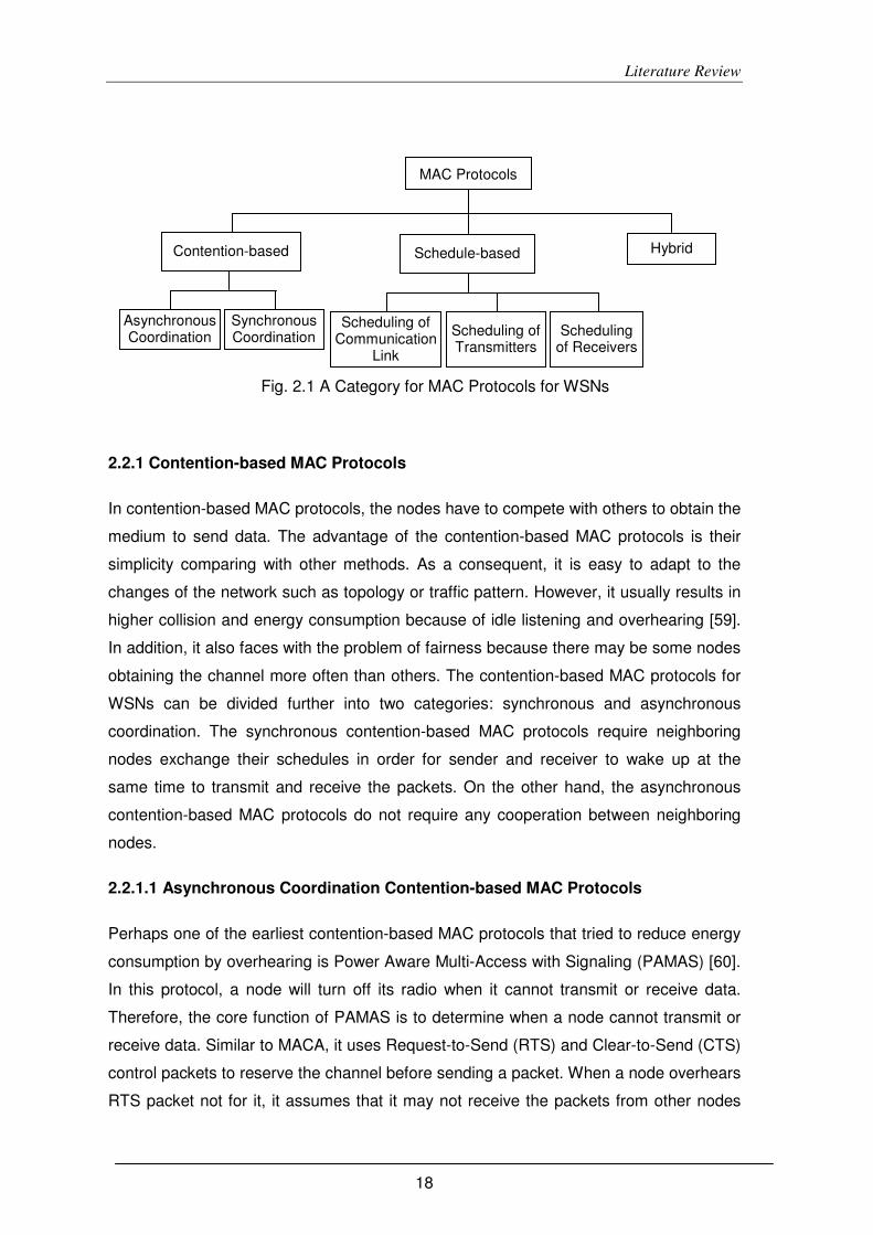
Literature Review
18
2.2.1 Contention-based MAC Protocols
In contention-based MAC protocols, the nodes have to compete with others to obtain the
medium to send data. The advantage of the contention-based MAC protocols is their
simplicity comparing with other methods. As a consequent, it is easy to adapt to the
changes of the network such as topology or traffic pattern. However, it usually results in
higher collision and energy consumption because of idle listening and overhearing [59].
In addition, it also faces with the problem of fairness because there may be some nodes
obtaining the channel more often than others. The contention-based MAC protocols for
WSNs can be divided further into two categories: synchronous and asynchronous
coordination. The synchronous contention-based MAC protocols require neighboring
nodes exchange their schedules in order for sender and receiver to wake up at the
same time to transmit and receive the packets. On the other hand, the asynchronous
contention-based MAC protocols do not require any cooperation between neighboring
nodes.
2.2.1.1 Asynchronous Coordination Contention-based MAC Protocols
Perhaps one of the earliest contention-based MAC protocols that tried to reduce energy
consumption by overhearing is Power Aware Multi-Access with Signaling (PAMAS) [60].
In this protocol, a node will turn off its radio when it cannot transmit or receive data.
Therefore, the core function of PAMAS is to determine when a node cannot transmit or
receive data. Similar to MACA, it uses Request-to-Send (RTS) and Clear-to-Send (CTS)
control packets to reserve the channel before sending a packet. When a node overhears
RTS packet not for it, it assumes that it may not receive the packets from other nodes
MAC Protocols
Contention-based Schedule-based Hybrid
Asynchronous Coordination
Scheduling of Communication
Link
Scheduling of Transmitters
Scheduling of Receivers
Synchronous Coordination
Fig. 2.1 A Category for MAC Protocols for WSNs

Literature Review
19
because the arrival packets will be collided with the sending packets from its neighbors.
Therefore, this node will turn off its radio if it has no packets to send. Similarly, when a
node overhears CTS message, it will turn its radio off because it knows that it cannot
send packets. The PAMAS can significantly reduce the energy consumption caused by
idle listening and overhearing. However, it is costly to implement and inappropriate for
WSNs because it uses two separate channels (radios): one for sending control
messages, i.e., RTS and CTS and the other for data messages [60]. In addition, during
receiving message time, the energy consumption of the receiver is almost double
because it has to issue the busy tone on the control channel to blocking its neighboring
nodes from initializing new transaction.
A more common approach for saving energy in WSNs is to use duty-cycle, i.e., the
nodes turns off its radio as much time as possible and only turns on its radio when they
have packets to transmit or to receive. For the asynchronous coordination MAC
protocols, each node independently chooses its active/sleep schedule. Because
neighboring nodes do not wake up at the same period, in order for a receiver to detect a
transmission, a preamble is prepended to a data frame. When a node wakes up, it will
sample the medium. If it detects a preamble, it will stay awake to receive the data,
otherwise it goes back to sleep immediately. It is important that the preamble should be
long enough for its intended receiver to wake up, detect it and receive the data. This
type of protocols is also called channel polling or Low Power Listening (LPL).
Berkeley Media Access Control (B-MAC) [61] is a preamble sample MAC protocol in
which the preamble is slightly longer than the sleep interval of the receiver to assure that
the receiver will wake up and receive the packet. To reduce the collision, B-MAC uses
backoff mechanism. In addition, to improve the efficiency of the clear channel
determination, it proposed a Clear Channel Assessment (CCA) method based on outlier
[61]. Furthermore, the active/sleep interval of a node can be configured to adapt with the
traffic load of the application. B-MAC significantly saves the energy wasted by the idle
listening, and control overhead. However, this protocol suffers wastes energy caused by
overhead of long preamble, and overhearing problem.
X-MAC [62] tries to reduce the overhearing problem of B-MAC by dividing the long
preamble into a series of short preambles. In addition, each short preamble also
includes the identification (ID) of the receiver. When a node detects that the incoming
packet is for it, it will send an early acknowledgement to inform the sender that the
receiver is awake and ready to receive the packet. As shown in Fig. 2.2, the early
acknowledgement will stop the sender from sending more preambles and thus it saves

Literature Review
20
energy. In addition, it also saves the energy from overhearing by using the ID of the
receiver.
Another preamble sampling MAC protocol for WSNs is Backoff Preamble Sequential
(BPS-MAC) [63], which uses a backoff preamble with variable length to reserve the
access to the medium. The primary objective of this protocol is to provide reliably data
exchange in dense WSNs. In this method, the interval during medium access is divided
into very short slots whose duration is equal or larger than the CCA delay duration [63].
When a node wants to transmit a packet, it senses the medium for three slots. If the
medium is free after the third slot, the node switches its transceiver from receive to
transmit mode. Then, it randomly chooses a length of the backoff preamble, which is
between one and the maximum backoff window, and transmits the preamble. After
transmitting the preamble, the node switches from transmit to receive mode to sense the
medium. If the medium is still free, the node switches its transceiver back to transmit
mode and starts transmitting the data. Otherwise, it switches off its transceiver and waits
for duration between two and the maximum backoff window before restarting the
process. The use of preambles with variable lengths reduces the collision. However, the
energy consumption of this protocol is very high because it does not use the duty-cycle.
Long preamble Data LPL Sender (S)
LPL Receiver (R)
Data
Data
Data
X-MAC Sender (S)
X-MAC Receiver (R)
Time
Time
Time
Time
A C K
extended wait time
Target address in data header
R wakes up Listen for queued packets
Receive early ACK Short preamble with target address
R wakes up Time & energy saved at S & R
Fig. 2.2 Comparison of timelines between LPL’s extended preamble and X-MAC’s short
preamble approach [62]

Literature Review
21
2.2.1.2 Synchronous Coordination Contention-based MAC Protocols
In this approach, nodes also employ the duty-cycle method, i.e., the node periodically
switches between active and sleep period, to save energy consumption. However,
differing from asynchronous coordination protocols, this method requires neighboring
nodes to be synchronized to wake up at the same time. Consequently, during the active
period, the neighboring nodes compete to gain the access to medium to transmit the
data.
Sensor MAC (S-MAC) [58] employs a fixed length active interval and a configurable
sleep interval, defined by its duty-cycle parameter. The active interval is divided into two
main portions: one for exchanging the SYNC packets and the other for transmitting the
data packets [58]. Each sub interval is further divided into smaller slots. In order for the
neighboring nodes to be able to communicate with each others, they have to wake up at
the same periods, i.e., common active periods. S-MAC employs a distributed method for
neighboring nodes to establish and synchronize their schedules. A node starts by
listening on the medium for duration at least one active interval plus one sleep interval. If
during this startup period, the node receives a SYNC packet, then it adopts the schedule
carried in that packet. Otherwise, it forms a schedule for itself by randomly choosing a
sleep interval. The node, then, broadcasts its schedule using the SYNC packet. To
maintain the schedule synchronization, each node consists of a table of its neighbors’
schedules, which are periodically broadcasted to the medium using SYNC packets [58].
In S-MAC, nodes transmit packets using the RTS/CTS handshake as used in MACAW
[57]. In addition, to avoid overhearing, a node turn its radio off when it detects that it
cannot neither transmit nor receive data as in PAMAS [60]. The packet of S-MAC
includes a duration field to help the neighboring nodes to decide their sleep duration.
Moreover, it also includes a mechanism that allows a node to reserve the medium for
transmitting long message called message passing [58]. One limitation of this MAC
protocol is that the schedule is decided beforehand, and it may be inefficient in real
networks. In addition, because the listening period of S-MAC is fixed, it may waste
energy if there is little or no traffic or it may be not enough when having heavy traffic.
Furthermore, the energy wasted by the control packets, i.e., SYNC, RTS/CTS packets,
is also high. Moreover, the collision is still high in dense WSNs.
A variation of S-MAC is Timeout-MAC (T-MAC) [64], which provides a mechanism to
adapt with variable traffic load by using an adaptive duty-cycle. When a node wakes up,
it listens for activity on the medium in a short duration and return to sleep mode when no

Literature Review
22
communication is observed. In addition, it employs a flexible active period that let a node
continue listening for a short interval after completing transmitting, receiving, or
overhearing a message. This allows the node to receive or transmit multiple packets
during its active interval. When a node has data to send but cannot transmit because the
channel is busy, it continues waked up until the channel becomes idle. This leads to the
early sleep problem, i.e., the intended receiver may return to sleep mode. T-MAC
resolves this problem by using Future Request-To-Send (FRTS) message [64] to inform
the intended receiver that there are incoming packets for it. This works as following:
when seeing the CTS on the medium, the node, which has data to transmit but cannot
do it, will send a FRTS message to request the intended receiver to stay awake. It is
important to note that the FRTS message may collide with the data message of the
neighbor transmitter. To solve this problem, after receiving CTS message the transmitter
transmits another dummy message called Data-Send (DS) to delay the transmission of
actual messages. However, this mechanism significantly increases idle listening and
thus wastes energy.
2.2.2 Schedule-based MAC Protocols
The schedule-based approach requires coordination among neighboring or all nodes to
reduce collision, idle listening and overhearing. Among the three common coordination
techniques for traditional MAC protocols, i.e., TDMA, FDMA, and CDMA, the first is the
highly used in WSNs. In addition, because their special characteristics, there are several
variations of TDMA schedule-based MAC protocols for WSNs. The MAC protocols in
this category can be divided into three groups: (1) Scheduling of communication link, (2)
Scheduling the transmitter, and (3) Scheduling of the receiver.
2.2.2.1 Scheduling of Communication Link
This is the traditional approach in which the time is divided into frames which in turn are
divided into slots. In each frame, each pair of neighboring nodes is assigned two slots:
one for transmitting and the other for receiving. The advantage of this traditional method
is that the internal collision can almost completely be avoided. In addition, the
overhearing and idle listening are minimized. However, in multihop WSNs the collision
may still happen because different paths may have different schedules. Another
disadvantage of this type of MAC protocol is that it requires a high accuracy time
synchronization, and thus increasing overhead. The scheduling mechanisms can be
either centralized or distributed.

Literature Review
23
The Traffic-Adaptive Medium Access (TRAMA) [65] is a distributed election scheme to
establish the schedules for nodes. In this protocol, each time frame is divided into
random and scheduled access periods. The former period is used for synchronization
and updating two-hop neighbour information while the latter one is used to contention-
free exchange data between nodes. The Neighbor Protocol (NP) is used to gather and
periodically update the two-hop neighbor information by using the signaling packets
during the random access period. The nodes use Schedule Exchange Protocol (SEP) to
exchange their schedules. For each time frame, every node computes number of slots it
needed and employs the Adaptive Election Algorithm (AEA) to decide which time slots it
can transmit. AEA computes the priority for a node at the time slot t using the pseudo-
random hash on the time slot ID and the node’s identification similar to that of used in
Neighborhood-aware Contention Resolution (NCR) [66]. Each node computes this
priority for all time slots for the node itself and all its two-hop neighbors, and it uses
those time slots for which it has the highest priority. Based on the schedules exchanged
using SEP protocol, nodes know when it should wake up to transmit and receive the
packets and when it should go to sleep to save energy. The nodes without any data to
send will give up the unused slots to its neighbors, thus, improving the channel
utilization.
Besides saving energy, this protocol also scales well because the schedule is computed
only based on the two-hop neighbors. In addition, it can also be easy to adapt to the
addition and removal of nodes. Moreover, it allows node to give up the unused slots for
other nodes and thus improving the throughput. However, the election algorithm is
complex. In addition, the overhead caused by control packets was very high. Moreover,
the delay of the packet may be long and unbounded. Furthermore, the fairness is also a
problem of this protocol.
DMAC [67] is designed for the data-gathering tree pattern, i.e., the traffic flow is from the
nodes to the sink. In this protocol, a “staggered wakeup schedule” is created for each
route from a leaf node to the sink as follows. During its sending interval, a node sends a
packet to the next hop on the route and waits for an acknowledgement. At the same
time, the next hop node is in receiving state and immediately follows by a sending state
to forward the packet to the next hop. This process is repeated until the packet reaches
its destination. DMAC minimizes the energy wastage by idle listening and overhearing.
In addition, it can guarantee a bounded delay. However, the collision between the
nodes with different parents, i.e., different paths, is still happen. In addition, its traffic

Literature Review
24
model is designed for sensor networks with static routes. Therefore, it cannot work well
for arbitrary flow between source and destination or when the data flow is changed.
Power Efficient and Delay Aware Medium Access Protocol for Sensor Networks
(PEDAMACS [68]) proposed a method for applying centralized TDMA for dealing with
the unplanned sensor network. It consists of three phases: topology learning, topology
collection and scheduling. In the first phase, each node collects information about its
neighbors and decides its parent node based on the control packets sent by the sink.
Then, the nodes send this information to the sink during the second phase. Based on
the gathered information, the sink calculates the schedule for all nodes in the network
such that in each time frame a node can transmit a packet to its parent without collision.
After finishing computing, the sink broadcast the schedule to the nodes. It is important to
note that the communication during the first two phases is contention-based and the
schedule is only for the uplink, i.e., only including the path from nodes to sink.
PEDAMACS minimizes the collision, overhearing, and idle listening. In addition, it gives
a bounded delay in a multi-hop network. However, besides the cost of control packets,
the limitation of PEDAMACS is that it assumes the sink is powerful enough to reach all
the nodes. This leads to the scalability problem. In addition, its performance is poor with
a large sensor network.
Ginseng MAC (GinMAC) [69], [70] is another TDMA MAC protocol which guarantees
reliable and timely data delivery while providing energy efficiency. It is used for multi-hop
WSNs with a pre-dimensioned virtual tree topology and hierarchical addresses. The
three main features of GinMAC are [69], [70]: off-line dimensioning, i.e., the network
topology and traffic patterns are defined before deployment; exclusive TDMA, i.e., a slot
used by one node cannot be re-used by other nodes in the network; Delay Conform
Reliability Control, i.e., it supports delay bounds of time to send data to sink and time to
send commands from the sink to actuators while achieving very high data transport
reliability. Similar to traditional TDMA, with GinMAC the schedule is computed by the
sink and broadcasted to the nodes. However, the topology and the maximum number of
nodes of the sensor network must be defined in advance.
In GinMAC, each node is aware of its position in the tree and knows the slot numbers
assigned to its child nodes and parent node, thus allowing it to transfer data in a
collision-free mode. However, because the time slots are exclusively used it reduces the
throughput. In addition, also has a problem with the scalability. Furthermore, if during its
receiving slot the node does not has data to receive; it wastes the energy by idle
listening.

Literature Review
25
2.2.2.2 Scheduling of Transmitters
The lightweight medium access control (LMAC) [71] is a TDMA-based protocol in which
every node based on its two-hop neighborhood information to choose a time slot for
itself. A node gets one slot in a frame to transmit packet, i.e., this method only creates
the schedules for the transmitters. In order to indicate the intended receivers of each
packet, a time slot is divided into control message (CM) and data message (DM). The
former is used to send control message that includes ID of the intended receivers.
When a node has data to send it waits until its allocated time slot and sends a control
message during the CM period. Every other node has to listen at the beginning time
slots of other nodes to check for incoming packets. If there is a packet for it, the node
will wake up during the DM interval to get the packet; otherwise it will go to sleep mode.
To establish the schedule at startup every node has to find a free time slot in its two-hop
neighbors and then randomly choose one of them. It does this by listening for the CM
from its neighbors, which contains a field named occupied slots indicating which slots
are occupied. By combining the occupied slots in CMs from its neighbors, a node can
find a list of free slot and randomly choose one of them. If there is a collision between
nodes, the involved nodes will restart the process of choosing time slot. This process
starts at the base station by randomly choosing a time slot and broadcasting it to the
network.
Because scheduling only based on the information from two-hop neighborhood allows
spatial reuse of the time slots, i.e., nodes whose distances are more than two-hops can
use the same time slot. It provides fairness among nodes in the network. However, the
nodes have to wake up at every time slot to check the destination of a packet, and thus
it will increase the idle listening. In addition, the schedule is only calculated once, it does
not adapt well to mobile sensor networks in which nodes regularly join and leave the
network.
The Mobile LMAC (MLMAC) [72] is an improvement of LMAC by allowing nodes to
update their schedules. In MLMAC, when two nodes are no longer receiving control
messages from each others, they will remove them from their neighbor lists. On the
other hand, when a node moves to new area, its old schedule might collide with a new
neighbor. If this happens, at least one node in their neighbor will recognize the collision,
and it will set the collision time slot as unused. This process forces the collision nodes to
restart their scheduling process. Because both these MAC protocols use fixed allocation
method, the bandwidth is not efficient used. In addition, control packet overhead also
high.

Literature Review
26
2.2.2.3 Scheduling of Receivers
In contrast to the scheduling of transmitters, this type of MAC protocols creates the
schedule for receivers, i.e., the node’s schedule is the time slot in which it will listen for
the incoming packets. It is important to note that scheduling of receivers is not collision-
free because at any time there may be more than one node to transmit packets to a
specific receiver. In this case, the transmitters have to contend to transmit the packets.
Pattern-MAC (P-MAC) [73] is contention-based and duty-cycle MAC protocol in which
nodes use patterns to describe its tentative awake and sleep time. The pattern is a
string of bits in the form 0m1, where m=0,1,…,N-1, and N is the period or the frame
length. The bits 0/1 represents the sleep and awake slot, respectively. For example, a
pattern of 0001 and N=8 indicates that this node will wake up at the slots fourth and
eighth of the period. This means that the pattern is repeated if its length is less than N.
Nodes exchange their patterns during a time interval called the Pattern Exchange Time
Frame (PETF) [73]. This pattern is only the tentative sleep-awake plan. The actual
schedule of a node also depends on its current traffic and the patterns of receivers. A
node always wakes up during bit 1 of its tentative plan to receive data. When a node has
data to send, it will wake up and attempt to transmit at the time slot of the receiver. The
node will go to sleep during other time slots. In order to save energy, during its time slot,
a node only wakes up at the beginning of that time slot and listens for a certain period of
time. If it hears nothing from its neighbors within that period, it goes to sleep again.
Although P-MAC can adapt to the traffic changes in the network, it does not improve idle
listening during active slots. In addition, the collision may be high when there is high
contention during a slot. Moreover, its control header is also high because of the pattern
synchronization.
O-MAC [74] is similar to P-MAC [73] in which each node independently selects its
reception slot. During its reception slot, the node wakes up and senses the channel. If it
detects a preamble then it remains active until it receives the whole packet [74]. In O-
MAC, the nodes are scheduled to wake up so that the neighboring receivers do not
interfere with each others. This protocol minimizes idle listening and overhearing but the
collision and overhead is still high.
Y-MAC [75] is another TDMA-based protocol, but it uses a multiple channels. Each time
frame is divided into broadcast period and unicast period. Each period contains a
number of time slots which further are divided into two parts: (1) contention window and
(2) message. Nodes wake up at the beginning of the broadcast period to exchange
Literature Review
27
broadcast messages, e.g., control messages to synchronize the schedules among
nodes. Each node is assigned a unicast slot to receive the data packets. When having a
packet to transmit, during the contention window of the time slot of the receiver, the
transmitter polls the base channel at a random time. If the channel is idle, it will occupy
the channel by sending a preamble to the channel until the end of the contention window
to suppress competing nodes. In order to further reduce idle listening, during its time
slot a node only wakes up at the end of the contention window to checks whether there
is any packet to receive.
In order to improve the performance (the throughput and delay), Y-MAC employs
multiple channels and light-weight channel hopping mechanisms to hop between
channels [75]. The advantage of this MAC protocol is that it can improve throughput and
reduce deliver latency using multiple channels. In addition, scheduling receiver
mechanism improves the energy efficiency. However, the overhead by control packets is
high. In addition, it works poorly in the heavy traffic conditions.
2.2.3 Hybrid MAC Protocols
The hybrid MAC protocols combine the characteristics of both contention-based and
schedule-based mechanisms. These protocols try to take the advantages of these types
of protocols and try to eliminate their limitations.
Zebra MAC (Z-MAC) [76] is a MAC protocol that combines the TDMA and CSMA. As
other distributed scheduling method, each node first collects information about its two-
hop neighbor nodes. Then, each node employs DRAND schedule algorithm [77] to
assign slots to every node in the network. DRAND ensures that no two nodes within
two-hop neighborhood are assigned the same slot. Each time slot is large enough to
transmit multiple frames. Z-MAC [76] has two operation modes depending on the
contention level. In a low contention level mode, nodes compete in all slots with different
priority. During its assigned slot, the owner has backoff time from 0 to T0 and other
nodes have backoff from T0 to Tn0. After the backoff time, the nodes sense the channel
to determine the channel conditions. In the high contention level mode, a node can use
Explicit Contention Notification (ECN) [76] messages to notify all nodes within two-hops
not to send during its time-slot.
Scheduled channel polling MAC (SCP-MAC) [78] is an ultra-low duty cycle which
combines the strengths of scheduling and LPL, and other optimal mechanisms to save
energy. Similar to other MACs, SCP-MAC also synchronizes the schedule with its two-
hop neighbors. In addition, it avoids idle listening and overhearing within the active

Literature Review
28
period through the sampling technique like that of used in X-MAC, i.e., including the
address of the receiver in the preamble messages. Moreover, SCP-MAC can also be
adapted to the traffic changes by additional wakeups that are added in the interval
between two regular wakeups.
The Mobility Adaptive Hybrid MAC (MH-MAC) [79] protocol is another hybrid MAC
protocol in which the scheduled–based approach is used for static nodes and
contention-based approach is used for mobile nodes. A frame is divided into time slots
which consist of two types: static slots and mobile slots. Each node estimates its mobility
by using a mobility estimation algorithm based on received signal strength [79], and it
uses a static or mobile slot depending on its mobility status. The nodes exchange its
mobility during the contention time at that start of frame. MH-MAC uses the same
mechanism as that of LMAC [71] to schedule static slots. For the mobile slots, the nodes
contend for using the medium in a two-phase contention period by using the preamble
sampling mechanism. Because all nodes have to wake up to sense the medium during
the mobile slots, it increases the energy consumption. In addition, the overhead is also
high because each frame includes first few slots for exchange mobility information of
nodes.
It is important to note that besides the internal collisions, there are other factors that
affect the communication in sensor networks including noise and interference from other
devices and networks. In addition, in real environments, there is probable that other
networks coexist with the sensor networks, which make it difficult to control the
operations and reliability of the sensor network. One current research direction that tries
to deal with these issues is Cognitive Radio (CR). The next section reviews current
research in this field.
2.3 Wireless network Coexistence and Cognitive Radio (CR)
2.3.1 Wireless Network Coexistence
As the wireless networks and devices become ubiquitous and many of them operate on
the same frequency band, interference happens almost everywhere. The interference
affects the performance of the involved networks and devices. As an example, the IEEE
802.11b/g/n and IEEE 802.15.4 compliant networks use the same 2.4 GHz band and
they may be deployed in the same area. The study in [1] showed that with the
interference caused by IEEE 802.11 based network the Packet Error Rate (PER) of
IEEE 802.15.4 was up to 95% when the interferer is in the distance of 1.5 meters.

Literature Review
29
Inversely, the throughput of IEEE 802.11 based network was reduced up to 30% when
the IEEE 802.15.4 based network in a short distance [2].
Yuan et al. [80] presented a model based on power and timing to evaluate the
coexistence of WLAN (IEEE 802.11b/g) and WSN (IEEE 802.15.4). In this work, the
CSMA/CA was employed and the CCA mechanism was used by a node to decide
whether or not to transmit a frame. Results from simulation showed that interference
between the networks was related to the power of transmission and the distance
between nodes and it severely affects the throughput of sensor networks. In addition,
Toscano and Lo Bello [81], [82] showed that even in networks consisting only of WSN,
interference still exists. Their test results on IEEE 802.15.4 based networks showed that
interference depended on the transmission power, on the distance between nodes and
on the duty-cycle. From these studies, it is important to note that interference is a hard
problem in coexistence of wireless networks, and it is necessary to have mechanisms
for different wireless networks to work reliable in the same area without affecting each
others.
Interference in wireless networks can be divided into two different types: co-channel and
adjacent channel. Co-channel interference is defined as the use of the same frequency
by more than one network or devices in the same area [83]. This type of interference
cannot be solved by increasing the signal power as that would increase the interference
and the communication problems in other neighbor networks. On the other hand,
adjacent channel interference occurs when consecutive channels are used by different
devices which lead to the degradation of both signals. That is the reason why channels
of a standard are separated in frequency to avoid interference. However, the separated
mechanism may not be sufficient because the filters and transceivers used by devices
are imperfect and they cannot cancel all the interference [83]. The effect may even be
more severe when transmitters and receivers from different networks using adjacent
channels are close to each other. To prevent this, better filters can be used in
transceivers and non-adjacent channels should be selected.
In order to deal with the coexistence of different wireless networks in the same area, the
IEEE 802.15.2-2003 work group [4] proposed a recommended practice for coexistence
of Wireless Personal Area Networks (WPANs) with other wireless devices operating in
unlicensed frequency bands, particularly wireless Local Area Networks (WLANs). This
recommendation suggests two approaches for coexistence between WLANs and
WPANs. The first approach requires the involved networks to collaboratively exchange
the information about the traffic patterns to mitigate the interference. However, the

Literature Review
30
problem with this approach is that it is necessary to have a communication link between
two networks. In addition, it requires a central control system to synchronize to grant the
access to the medium. The control mechanisms could be timing or on demand.
Moreover, it is difficult to realize in real environments.
The second approach is to use non-collaborative mechanisms in which no common
communication link between the two types of networks is required. The possible
techniques that can be used in this approaches are adaptive packet selection and
scheduling, signal processing, adjust packet size depending on the condition of channel,
and channel hoping [4]. Recently, the IEEE 802.19 work group [84] was created to
continue the previous recommendations and to develop a standard for coexistence
between wireless devices operating in unlicensed band.
The work in [85] illustrated the utilization of the collaborative mechanism for allocating
channels among WSNs. The network model in this study consists of a central entity and
the WSN coordinators. It is assumed that all WSN coordinators have wireless and wired
interfaces and that the communication to the central entity is made using an Ethernet
network. Results showed that this mechanism could be used to allocate the resources
(i.e., the channel) to sensor nodes and allow coexistence among WSNs. However, this
mechanism is only validated with simulation. In addition, it only works for the same types
of networks (i.e., WSNs). Consequently, it cannot deal with the interference from other
wireless devices.
Zhou et al [86] experimentally demonstrated how electronic devices operating at 2.400
MHz can cause interference and even hinder the operation of the IEEE 802.15.4 based
WSNs. To avoid this, the authors proposed a multi-channel approach for WSNs, which
have multi-frequency radios. They also proposed a middleware between the physical
and MAC layers in order to support multiple channels. However, this model was not
validated.
Frequency Hopping Spread Spectrum (FHSS) can be used as an alternative solution to
the coexistence of WSNs. According to [87], channel hopping can reduce interference
and increase resilience between neighborhood networks. However, this mechanism
uses a pseudo-random sequence to make the frequency hops and does not consider
the quality of different channels. If interference exists in more than one channel, FHSS
technique may result in loss of packets and intermittent disruptions.

Literature Review
31
2.3.2 Cognitive Radio (CR)
A more recent technique for flexible and efficient usage of radio spectrum is Cognitive
Radio (CR) [88]. The objective of CR is to allow secondary devices to opportunistically
access the radio channel without affecting the primary users. One of the main
characteristics of CR is the ability to change the radio parameters (including frequency,
power, modulation, bandwidth) depending on the radio environment, user’s situation,
network condition, etc [89]. Consequently, it is important to have such a kind of radio
that enables dynamically reconfiguring these parameters by software; and this type of
radio is called Software Defined Radios (SDR) [5], [89]. CR is based on Dynamic
Spectrum Allocation (DSA), or Opportunistic Spectrum Allocation (OSA) scheme to
improve the usage of the radio spectrum. The main functions of CR are sensing,
management, mobility, and sharing the spectrum [5]. These functions help to indentify a
best channel or available hole for devices or networks to use at current time
Dynamic Spectrum Access Protocol (DSAP) [90] is a collaborative protocol for
coexistence with central coordination. It is designed to be used in limited geographical
areas and aims to lower the congestion and interference between networks by adjusting
the channels used by the nodes, according to information provided by the central
coordinator. To accomplish this, management coordinators must have previous
knowledge of the channels in use in the region. The coordinators use two interfaces,
one to have a common channel to communicate with its client nodes and other to
access the information about the channel usage in the region. Results show that the
DSAP reduces interference and improves the throughput. However, a wrong choice of
the common channel or the effects of noise in the communication environment may
disrupt the communication between nodes.
The study in [6] showed that it is possible to apply DSA models for WSN to efficiently
use frequency spectrum and to support the coexistence of the networks. To accomplish
that, CR explores the frequency spectrum using an opportunistic mode, adjusting the
transmission parameters (frequency, transmission power and/or codification) based on
the information gathered from the environment. Other approaches using CR are
discussed in [5], [88] and propose that CR, besides the programmable reconfiguration,
may also learn to adapt to the surrounding environment by reconfiguring, in an intelligent
way, all the transmission parameters.
A framework for employing CR for WSNs, named Cognitive Radio Sensor Networks
(CRSN), was proposed in [91]. In this work, the authors developed two spectrum

Literature Review
32
decision protocols for applying CR mechanism for WSNs. These protocols employ
distributed mechanisms to select the best wireless channel based on the application’s
Quality of Service (QoS) requirements. Simulations of low, medium and high noise
scenarios have shown that the protocols improve the delivery rate while keeping the
delay and energy consumption unchanged. However, the works in [91] only validated
using simulation, its applicability for real WSNs is a question and needs more efforts to
realize. In addition, the proposed protocols are based on CSMA/CA whose response
time is not deterministic and therefore are not suitable for critical environments.
Although cognitive radio is a potential mechanism for coexistence, the full CR may be
too complicated for sensor networks. Therefore, it is necessary to have simpler
mechanisms for WSNs to coexist with other wireless networks while providing an
acceptably reliable communication. In addition, the coexisting solution should also take
into account other noise sources such as machineries, engines, and turbulences.
2.4 Integrating Sensor networks With External Environments
Although there are numerous potentials, WSNs are useless if operating in isolation. It is
clear that the sensed data must be collected, processed and visualized by some
applications to make them meaningful to users. In addition, the sensed data could be
mashed up with other data resources via web to create new applications. Moreover, the
sensor nodes and networks can also be remotely monitored and controlled by users
through front-end applications. Consequently, interoperability between sensor networks
and external environments is an undeniable requirement. Realizing this requirement will
make WSNs an important component of the future Internet and integral part of our lives.
The following subsections reviews the current works on interconnection and integration
approaches for WSNs as well as discusses their advantages and limitations.
In this thesis, the term external application refers to an application such as Supervisory
Control and Data Acquisition (SCADA), enterprise application, or application platforms
such as web 2.0. In addition, the term external network refers to the networks other than
sensor network such as LAN or Internet. Moreover, the term external environment refers
to both external application and network.
2.4.1 Internetworking
The approaches for interconnecting WSNs with external networks can be divided into
two main categories: Gateway-based and IP-based.

Literature Review
33
2.4.1.1 Gateway-based Approach
As sensor networks are very different from the IP-based networks, the common
approach to interconnect them is to deploy one or more gateways or proxies between
the two dissimilar networks. Different gateway-based methods have been proposed for
connecting WSNs with external networks.
2.4.1.1.1 Application-level Gateway
In this approach, the gateway or proxy translates and forwards the packets between two
networks. The gateway or proxy can act as a relay or as a front-end [7]. In the relay
mode, when receiving a message from sensor network, the gateway/proxy simply
translates and relays it to the client applications on TCP/IP network. In order to know to
destinations to forward the messages, the clients must register for the particular interest
data with the gateway. On the other hand, in the front-end mode, the sensed data are
collected and stored in the database on the gateway, and the clients then query it for the
required information.
The main advantage of application-level gateway is that it completely decouples two
types of networks. This makes them totally transparent to each other, i.e., the client
applications can use the sensed data without knowing details about sensor networks. In
addition, it is simple to implement. Furthermore, some security features such as
authentication and authorization can be implemented with the front-end gateway
approach. However, the application-level gateway is usually for specific tasks or a set of
specific protocols, i.e., it requires a specific gateway or proxy for each sensor network
[7]. In addition, conventional application-level gateway does not support direct access to
individual sensor nodes. Furthermore, the gateway is the single-point of failure, i.e., if
the gateway fails, then the communication between two networks becomes impossible.
In order to allow direct access to individual sensor nodes from the Internet using
application-level gateway, Kim et al [11] proposed a scheme for assigning IPv6
addresses to sensor nodes. In this method, the gateway maintains a table of mapping
between IP address and sensor node’s identification information such as network ID and
sensor ID.
2.4.1.1.2 Low-level Gateway
Low-level gateway is another approach for interconnecting sensor networks with
external networks. Differing from the application-level gateway, in this approach the
Literature Review
34
gateway does not translate the content of the packets but it only translates the lower
level header information of the packets between these two networks.
Shu et al. [12] proposed an approach for interconnecting several isolated heterogeneous
WSNs with IP-based networks to form a virtual sensor network named VIP Bridge. VIP
Bridge was based on the node-centric or location-centric communication paradigm to
map node IDs to IPv6 addresses. Because the TCP/IP protocol stack was not
implemented on the sensor nodes, the IP addresses of sensor nodes were stored on the
VIP Bridge. Similar to the application-level gateway, the packets that comes from one
side is translated into the corresponding format and sent to the other side by the VIP
Bridge. However, VIP Bridge is not an application-level gateway but a low-level
gateway, i.e., it does not translate the content of the packets but only makes a mapping
between IPv6 addresses and sensor node IDs and routes the traffic between these two
networks.
The main advantage of this approach is that Internet applications can directly access to
the sensor node using IP addresses. This makes the sensor networks transparent to the
Internet users, i.e., sensor nodes are viewed as normal IP hosts. In addition, the
communication protocols in WSNs could freely be chosen. However, this approach has
several limitations. First, it requires the sensor nodes to register their IDs or location
addresses as well as the essential information with VIP bridges. In addition, the client
applications are WSNs-specific, i.e., they must have the ability to understand and
analyze the payload of the WSN packets. One more drawback is that the packet
analysis and translation are based on a specific field to categorize the packets into
operation or query commands (O/Q) or data or acknowledgement (D/A) [12]. As a result,
the VIP Bridge regulates its own packet format for communication between WSNs and
IP networks, i.e., this solution cannot be deployed for existing sensor networks and
applications. Furthermore, creating and sending multiple packet to WSNs for a data
query is not efficient.
Another low-level gateway that bases on the idea of VIP Bridge with some
improvements was proposed in [10]. First, it does not require sensor nodes register their
information to the gateway. Second, it does not use a specific field to identify the type of
commands (operation or query). Therefore, it also does not require modification of user
and sensor applications. In addition, it supports the data-centric WSNs by assigning a
virtual IP address for a specific interest similar to multicast IP. Furthermore, it also
provides two-way communication by assigning virtual sensor node IDs for IP hosts.
However, this approach has several drawbacks. First, the low-level gateways assume

Literature Review
35
that the application protocol is the same on both sides. This makes the sensor networks
not totally transparent to Internet host. This also means that the low-level gateway
approach requires that the user applications must have ability to analyze the packets
from the WSNs to get the useful data. Furthermore, these frameworks are not well
support for data-centric network, i.e., one-to-many and many-to-one data flow.
2.4.1.2 IP-enabled WSNs
Because of the resource-constraint of sensor nodes many researchers assumed that it
was unfeasible or inefficient to deploy TCP/IP protocol stack directly into sensor nodes
[8], [10], [12]. However, the micro IP (uIP) implemented in [14] proved that it is possible
to implement the TCP/IP stack on the sensor nodes with limited memory and
computation. In addition, Dunkels et al. [21] introduced some optimization mechanisms
such as spatial IP address assignment, header compression, application overlay routing,
and distributed TCP caching for adapting TCP/IP protocol stack for WSNs. These works
laid groundwork for exploring the use of TCP/IP for WSNs.
In recent years, IPv6 for sensor nodes has attracted a lot of attention of the research
community because of its huge number of addresses and its simplicity. In order to apply
IPv6 for sensor networks, 6LoWPAN [15], [92], [93] proposed an adaptation layer
between link layer and network layer to enable efficient IPv6 communication over IEEE
802.15.4 links. In addition, it also proposed a cross-layer optimization with three primary
elements: hear compression, fragmentation and layer-two forwarding. Currently, both
TinyOS [94] and Contiki [95], the two most common operating system for WSNs, include
an implementation of the 6LowPAN [15].
Incorporating IP directly in sensor nodes makes the interconnection between sensor
nodes and the Internet easier and more natural, i.e., the Internet host can directly
communicate with the sensor nodes. It is the crucial step to realize the vision of Internet
of Things (IoT). However, its efficiency in terms of energy and usefulness as well as its
suitability and applicability for WSNs still needs more investigation. The most obvious
issue with this approach is that it is not suitable for data-centric sensor networks, where
the routing is based on the contents and not on the addresses of sensor nodes. In
addition, security is also a big issue. Furthermore, adaptation layer and other optimal
mechanisms make 6LoWPAN [15] incompatible with conventional IP network.
Consequently, it still needs a bridge/router/gateway between WSNs and IP networks.
Although the studies have shown that it is possible to deploy TCP/IP protocol stack into
sensor nodes, both approaches (gateway-based and IP-enabled) for interconnecting

Literature Review
36
WSNs with the external networks have been continue co-existing. In some case, IP-
based approach is more appropriate but in others gateway-based must be used.
Furthermore, the combination of gateway-based and IP-based approaches is also
possible.
2.4.2 Integration
Interconnecting sensor networks with external networks opens the gate for realizing the
IoT. However, because the primary functions of a WSN are to sense or gather the
physical data and to activate things, it needs to be monitored and controlled by other
applications. In order to allow a seamless interoperability between sensor networks and
external applications, it is necessary to have another abstraction layer. This means that
it needs an infrastructure for simplifying the data exchange between sensor networks
and external applications.
The current work on integrating sensor networks with external applications can be
approximately categorized into two groups: direct access and Indirect access. The
following subsections review the research on these areas.
2.4.2.1 Direct Access Approach
One research direction on integrating sensor network with Internet and external
applications is to treat the sensor nodes as the normal nodes of the IP based network.
This means that each node has a unique IP address, a web server, and/or a Web
service API. In this approach, each sensor node is treated as an information server [18],
and it can be directly accessed from the Internet.
One of the early works on this approach was Tiny Web Services [17], which employed
uIP [14] and Web services for sensor nodes. Because the standard implementation of
Simple Object Access Protocol (SOAP)-based web services [96] is unlikely to be
suitable for sensor nodes, Tiny Web Services employed numerous optimization
mechanisms to reduce overhead and delay [17]. First, the TCP persistent connection
was used to reduce the number of TCP messages in each call. In addition, TCP
acknowledgements were disabled to reduce delay. Furthermore, to support end-to-end
reliability, link layer retransmissions were employed instead of transport layer. Moreover,
the low power mode between TCP messages could also be used to improve the energy
efficiency. Notably, although, the Hypertext Transfer Protocol (HTTP) binding is used to
remove the SOAP envelopes from the messages, the sizes of messages are still too
large for constraint devices. Therefore, Tiny Web service [17] employed a context based

Literature Review
37
compression method in which the method name was replaced by its compact tag, i.e., a
number. For supporting duty cycled nodes the WS-Eventing [97] was implemented at
the gateway. A prototype was implemented to prove that it was possible to use Web
service for resource-constrained sensor nodes. However, despite the payload of the
message being compressed, it was still very large when compared with the bare-bone
protocol. In addition, because Tiny Web Services [17] employed the generic
compression algorithms and supported cycled duty, it still required an HTTP proxy
between the client applications and sensor nodes.
Another work that implemented an embedded IP stack and HTTP server on each node
to make its sensors and actuators available through web service API was introduced in
Web of Things (WoT) [19]. Different from Tiny Web Services [17], this work employed
Representation State Transfer (REST) [98] based web service, i.e., it was built on top of
HTTP and uses JavaScript Object Notation (JSON) [99] instead of eXtensible Markup
Language (XML) [100] for formatting messages. Because the work in [19] did not
employ any optimization mechanisms for reducing the overhead, it is possible for user
applications to directly access sensors’ data and functionalities. However, although
RESTful web service [98], [101] is more compact then XML based web service, it is still
inappropriate for many constraints sensor nodes. In addition, it is difficult and inefficient
to implement both standard TCP/IP stack and traditional web services on sensor nodes.
In fact, the current implementations of this work was not included the TCP/IP protocol
stack. Consequently, a proxy and gateway is still needed to access the web service API
implemented on the sensor.
A similar work to [19], which implemented RESTful web service on the sensor nodes,
was sMAP [18]. However, sMAP targeted at the representation and transmission of the
physical information. Particularly, it defined a hierarchical organization for the
information. In addition, the web service on each node also provided the necessary
information for interpreting the sensed data. Moreover, to make the message more
compact for sensor nodes, sMAP employs the adaptations at different layers for running
on constraint devices including 6LowPAN [15] at network layer, User Datagram
Protocol (UDP) [102] at transport layer, Embedded Binary HTTP (EHTTP) [103] for web
instead of HTTP, and packed JSON [18]. Similar to previous works, the proxy and/or
gateway was still needed for the communication between the user applications and
sensor networks.
Literature Review
38
2.4.2.2 Indirect Access Approach
This approach refers to the integration methods that comprise one or more gateways or
proxies sitting between the sensor networks and the client applications. The gateway
provides a set of web service API for the client applications to access the sensed data
as well as to communicate the commands to the sensor networks.
Global Sensor Networks (GSN) [13] proposed an infrastructure for data integration from
multiple sensor networks through the virtual sensor abstraction. The virtual sensor
receives and processes the input data from the real sensors or other virtual sensors to
produce a unique output. Which input data and how they are processed to create the
output is described by the virtual sensor description. This way, the virtual sensor
abstracts the details of access to the sensor data. The input and output data structure
are described using XML, and Structured Query Language (SQL) syntax is used to
describe how the input data are manipulated to produce output. Consequently, GSN
[13] can help to integrate data from multiple sensor networks, and to hide the details of
sensor networks from client applications. In addition, it also allows client applications to
easily combine the sensed data as other traditional data sources. However, in order to
feed the input data to GSN, a software wrapper is needed for each specific type of
devices and for each data frame structure.
Inspired by the success of Web 2.0 paradigm, researchers have tried to leverage this
model for integrating sensor networks with the applications. This means that the sensed
data and sensor nodes can be treated as traditional data sources, i.e., they can be
easily accessed by applications, e.g., via web service API or using a browser.
SenseWeb [104] was such an approach which proposed an infrastructure for sharing
sensor data in order for them to be consumed or mashed up with other applications. It
provides a Web Services API for applications to access shared sensor data. In addition,
to communicate with sensors, it comprises a gateway, called DataHub [104], and drivers
to communicate with sensors. Moreover, it also includes mobile proxy for
communicating with mobile devices such as mobile phone or sensor attached to
vehicles. Furthermore, in order to add semantics to the data, it also consists of a set of
transformers to convert raw data to suitable format as well as adding the description to
it.

Literature Review
39
2.4.3 Comparison of the Integration Methods for WSNS
This section makes a comparison among the current approaches for integrating WSNs
with the external environments. This comparison is mainly based on the features that an
integration solution should provide. It is important to note that the 6LowPAN [15] is not
included in this comparison because it is considered as the infrastructure for other
higher layer integration solutions. In addition, the application level gateway in this
context is the traditional gateway, i.e., it simply translates the messages between two
different types of networks.
In this comparison:
- “Potential” means that it is possible to provide such features but it was not
considered or implemented in traditional methods.
- “Partial” means that the proposed solution does not fully support the feature.
The “transparency” feature in this context means that the details of sensor nodes and
networks are hidden from the external applications. In addition, the changes inside the
WSNs (e.g., adding new frame format, changing routing protocols, etc) should be hidden
from the client applications. What the application needs to know is how to obtain
required data or how to send command to the sensor network(s). VIP Bridge [12] only
provided virtual IP address for sensor nodes, it did not hide the higher layers from
Application level
gateway
VIP ridge [12]
Tiny Web Service
[17]
WoT [19] sMAP [18] GSN [13] and SenseWeb
[104]
Transparency Yes No Yes Yes Yes Yes
Interoperability Potential No Yes Yes Yes Yes
Freely choose optimal protocols
for WSNs
Yes Yes No No No Yes
Individual node access
Potential Yes Yes Yes Yes Yes
Easy Integration Potential No Yes Yes Yes Yes
Data-Centric Potential No No Partial Partial Yes
Adaptability Potential No Partial Partial Partial Partial
Table 2.1 Comparison of Different Approaches for Integrating WSNs and External
Environments

Literature Review
40
applications. In addition, it required modifying the sensor node applications to register to
the gateway.
The second feature, interoperability, means that the integration solution should follow a
well-known encoding format for exchanging information. In addition, the contents
presented in the message are correctly understood by the applications, i.e., semantics.
Moreover, it should also provide a standard interface for accessing sensor networks.
The Internet host's applications can interact with WSNs using the similar methods that
are used to interact with other software components, e.g., using web services. The first
two methods in Table 2.1only concentrate on interconnect the two types of networks,
and it leaves the user applications to analyze and interpret the sensed data. On the
other hand, the remaining solutions exposed the sensed data using web services. In
addition, it could also include the semantics for the sensed data, as an example, sMAP
[18] comprises description for the representation of data. Consequently, it is very easy
for the user applications to interoperate with WSNs.
Because the sensor nodes have very limited resources, the integration solutions should
maintain the optimization mechanisms for the sensor networks, i.e., the developers can
freely choose protocols that best fit for the specific deployment. Because the Tiny Web
service [17], WoT [19], and sMAP [18] directly deployed web services on sensor nodes,
it limits that the optimization mechanisms can only be related to TCP/IP and web
services. Therefore, it is difficult or impossible to choose the optimal protocols for WSNs.
The other solutions do not intervene in the internal operations of sensor networks;
therefore, they are free to choose the protocols to be used in WSNs.
In this section, “individual node access” means that Internet hosts can directly send
commands to individual sensor nodes using some types of identification, e.g., IP
address. This type of access is required for remotely manage purposes such as
monitoring, reprogramming, reconfiguring nodes (e.g., control sensing and report
functions) or actuating other systems. Among the current approaches, implementing
web services on sensor nodes naturally provides access to individual sensor node.
Similarly, low-level gateway [12], which assigns a global unique IP for every sensor
node on the bridge, also allows to directly access to individual sensor node using its
virtual IP address. Meanwhile, it is assumed that application-level gateway does not
provide direct access to sensor nodes. However, it is possible to adopt this functionality
into application-level gateway to provide access to individual sensor nodes.
One crucial requirement for integration solution is that it is easy for the applications to
access and consume the sensed data. By exposing the sensed data using web service

Literature Review
41
API, e.g., Tiny web service [17], WoT [19], sMAP [18], and SenseWed [104] make the
interoperability between sensor networks and applications easy. They allow the physical
information available to be mashed up with other data source via web. Other solutions
require the application to know how to analyze the message from the sensor networks.
However, the application-level gateway could include the web services to expose the
sensed data; and therefore, it can make the integration with external applications easier.
Data-centric, named data query, is one of the typical features of WSNs. It is also a
challenge for integrating WSNs with IP-based networks. The approach embedding
HTTP servers and web services into sensor nodes mainly focuses on providing access
to individual sensor nodes, and do not dedicate much attention towards methods for
querying sensor networks (data-centric). Although VIP Bridge [12] allows to send
queries, it only allows to send individual sensor nodes. Additionally, it does not provide a
mechanism for processing and aggregating the result data. The gateway-based
approach, .e.g., GSN [13] and SenseWeb [104] can supports data-centric for WSNs.
Adaptability feature refers to the ability of the integration solution to be able to adapt to
different types of protocols and data frame formats of sensor networks. It is an important
requirement because there is a large number of protocols and a frame formats
developed for WSNs, and the numbers have never stopped increasing. In addition, the
sensed data is not consumed directly by end users but by other applications. This leads
to a small change in data format could lead to totally different packet for the client
applications. Because web service in sensor nodes sits on top the communication layer,
this approach adapts well with the diversity of protocols and data formats of sensor
networks. VIP Bridge [12] cannot adapt well with the changes in sensor networks
because they needs to know the detail of the protocols to make the conversion. In order
to add a new type of sensor, or data format frame, it is necessary for the gateway-based
solution to have new modules or drivers to deal with this change.
From the analysis in this section, we recognize that in order to seamlessly integrate
WSNs with external applications, the integration solution should take into account the
requirements mentioned in Table 2.1. The integration infrastructure should be able to
adapt to different data formats of WSNs without reprogramming. As adaptability is an
important feature and it is not resolved by the current gateway-based, the integration
framework in this thesis tries to propose a solution for this problem. In addition, the
interoperability is also a primary focus.
Literature Review
42
2.5 Localization
Localization is the process of determining the positions of devices, objects, things or
people within an area of interest. Localization in wireless networks (including WSNs) is
an important area attracting considerable research and development both in academia
and industry. It is especially important in WSNs because the measured data are
meaningless without knowing the location from which the data are obtained. In addition,
many important and useful applications, e.g., rescue, target tracking and monitoring, and
health-care, need information about the place in which the events happened, i.e., the
position of the objects involved in the events. Furthermore, the positions of nodes can
be used in routing algorithms and for reducing power consumption mechanisms.
In order to estimate the position of unknown position objects (e.g., sensor nodes), the
localization algorithms need some inter-sensor measurement, e.g., the signal strength,
the angle, or the propagation time. In addition, in most cases, it is necessary to have the
presence of a number of known position nodes called anchors, reference points or
beacons. Based on different assumptions and applications, numerous localization
algorithms have been proposed for WSNs. Although using different algorithms and
having different requirements, the localization systems usually comprise two main
phases: measurement and position estimation. In each phase, there may be one or
more steps depending on the localization algorithm. During the measurement phase,
data useful for the localization purpose are obtained from the network. The measured
data are then used by the location algorithms to estimate the position of the object in
second phase.
This section reviews the measurement techniques that are practically feasible in
wireless networks and major localization algorithms that were proposed so far for
determining the positions of nodes in WSNs.
2.5.1 Measurement Techniques
In order to determine the position of a device, it is necessary to have some
measurement between nodes or between a node and several anchors in the network.
The common measurement methods that can be used in estimating the position of a
device in a wireless network are Received Signal Strength Indication (RSSI),
Propagation time, and Angle-of-Arrival (AOA). This section reviews these measurement
methods and discusses their strengths and limitations.

Literature Review
43
2.5.1.1 Received Signal Strength Indication (RSSI)
Perhaps the simplest and cheapest measurement method is RSSI because it is easy to
measure and is available in almost every wireless network including WSNs. RSSI is the
magnitude of the power of the signal received at the receiver. Theoretically, by using
RSSI, the transmitted power, the gain of antennae at the transmitter and receiver, and
the propagation model, it is possible to estimate the distance between the transmitter
and receiver. However, because the propagation characteristics of the channel change
from place to place and from time to time [105], it is very difficult to find a good
propagation model for a specific environment. In addition, there are a number of factors
that affect the quality of the received signal strength including pathloss (i.e., attenuation
and the effects of the propagation channel), shadowing (e.g., absorption, reflection,
scattering, and diffraction caused by obstacles between the transmitter and receiver)
[106], interference, noise, and even the quality of the devices (e.g., anisotropy and the
sensitivity of the antenna) themselves. These factors make the RSSI value be unstable
and unreliable. As a result, it is high inaccurate to estimate the distance using RSSI
value.
2.5.1.2 Propagation Time
Signal propagation time, also called time-of-flight, is the time taken by a signal to travel
from the transmitter to the receiver. It is possible to use the propagation time to estimate
the distance between two devices because the propagation speed of signal in the
medium is usually known in advance. For instance, the sound signal travels at the speed
of 344 meters per second in dry air at 21◦c; or radio signal travels at the speed of
299,792,458 meters per second [107]. There are several different techniques that can
be used to measure the propagation time including Time-of-Arrival (ToA), Round-trip
time-of-flight, combining radio signal and Ultra-sound, and Ultra-wide band (UWB).
Time-of-Arrival (ToA): ToA measures the difference between the time at which a signal
is received (arrival) at the receiver and the time that signal was transmitted by the
transmitter [108], [109]. In order to compute this time difference, it is required that the
transmitter has to timestamp the frames when sending them. More importantly, the local
time of transmitter and receiver must be very accurately synchronized. However,
because the travel speed of radio signal is very fast and WSNs only communicate in a
short distance, it demands that sensor nodes have a very high accurate clock and more
complexity algorithms to have the high accurate synchronization, i.e., nanosecond (ns).
Consequently, ToA is not a suitable measurement method for WSNs.

Literature Review
44
Round-trip time-of-flight: This method to measures the difference between the time a
frame was sent by a node and the time that frame arrived back to it [108], [109], [110].
Although the time synchronization is not required, because the same clock is used,
there are still several sources of errors. First, the waiting times at the transmitter and
receiver, i.e., the duration that the frame is in queue because channel is busy. In
addition, the processing time of MAC protocol and higher layers is usually difficult to
compute. Moreover, the precision of hardware packet timestamp also contribute to the
accuracy of this measurement method. Furthermore, other factors such as Non-Line of
Sight (NLoS) also significantly affect the accuracy of measurement. Finally, because
this method requires multiple frames to be exchanged between unknown position device
and anchors, it is difficult to use in localization algorithms for highly mobile nodes.
Combination of Radio and Ultra-sound signals: A more accurate but more costly
method for measuring propagation time without time synchronization is to combine
Radio Frequency (RF) signal and Ultra-sound signal [26]. In this method, the transmitter
sends both the RF signal and ultrasound pulse at the same time. Because the speed of
RF signal is very fast comparing with that of Ultra-sound pulse and the communication in
WSN is in very short range, the RF signal could be considered as instantaneously
received at the receiver without any delay. Consequently, the propagation time can
approximately be calculated as the difference between the arrival time of Ultra-sound
pulse and that of RF signal. The advantage of this method is the accurate estimate of
the propagation time. However, it requires the additional hardware which is costly and
energy inefficient for WSNs. In addition, the Ultra-sound is severely affected by
obstacles, multipath and other noise sources.
Ultra-wide band (UWB): A signal is considered as an UWB if its total bandwidth is more
than 500 Mhz [111]. It is a new wireless technology for short-range high bandwidth
communication with a low energy level. The characteristics of UWB signal can be
exploited to improve the accuracy of the propagation time measurement. In addition,
[112] proposed to use generalized maximum-likelihood (GML) estimation for detecting
the direct path of the signal. The process of measurement of propagation time is the
same as that of ToA or round-trip time of flight. Therefore, this method also has the
same issues as those of these two techniques but it is more accurate.
2.5.1.3 Angle of Arrival
Angle of Arrival (AoA) technique measures the angle of the received signal at a
measurement unit [113]. Based on the angles obtained from measurement units, the

Literature Review
45
location of the devices can be estimated by localization algorithms. The AOA techniques
can be divided into two subclasses: amplitude response and phase response [108]. The
former uses the amplitude while the latter exploits the phase of the received signals to
infer the angle. A common technique in both these approaches is to use an array of the
antennae (at least 2 antennae).
The amplitude-based approach exploits the anisotropy in the reception pattern of
antennae, i.e. the antenna is not uniform in all direction – the same transmitted signal
has different strength if received by the different directions, to infer the direction and thus
the angle of the transmitted signal. In [114], an array of antennae is used to measure the
angle by comparing the received signal strengths received at different antennae and
overlapping the reception patterns of the antennae.
Similar to amplitude-based approach, the phase-based approach also uses an array of
antennae at the receiver but it measures the phases of the signals instead of the
strengths of received signals at different antennae. Phase interferometry discussed in
[115] uses an array of antennae separated by a uniform distance to measure the
phases of the transmitted signal. The signals received at different antennae have
different phases and this information is used to estimate the angle or direction of the
transmitter.
The AOA could produce an angle measurement with an accuracy of up to 2 degrees.
However, it requires an array of antennae, which is more expensive than the normal
one. In addition, the accuracy of this method relies on the Line-of-Sight (LoS) path from
the transmitter and receiver. Therefore, it is severely affected by shadowing, multipath
and obstacles.
Having reviewed the potential measurement methods in WSN, the next section presents
methods which can be used for estimating the positions of sensor nodes in WSNs.
2.5.2. Localization Methods
There are numerous ways to categorize the localization methods based on different
criteria such as whether or not the algorithm requires the distance measurements
(range-based and range-free); whether or not it needs the beacons (beacons and
beaconless); whether or not it supports mobile nodes, etc. In this review the localization
algorithms are divided into two main groups: one for ad-hoc sensor networks and the
other for controlled ones. As shown in Fig. 2.3, in each main category, the algorithms
are further divided into different types depending on mathematical model or algorithm

Literature Review
46
type. It is important to note that some localization methods could apply to both types of
sensor networks such as lateration, SVM, etc.
Almost all of the localization algorithms assume that a proportion of nodes in the
network have fixed known positions. These special nodes are called different names
such as anchors, reference nodes, beacons or landmarks. In the following subsections
these terms are used interchangeable.
2.5.2.1 Localization Methods for Ad-hoc Sensor Networks
Based on the original concept of WSNs, i.e., a large number of small and inexpensive
sensor nodes are wirelessly connected together to form a network with the useful
functions for monitoring and controlling the physical environments [116], one research
direction targets localization problem with assumption that sensor networks are static or
semi-static. This means that the sensor networks will be deployed by randomly
scattering nodes on the area of interest (e.g., forest or battle field). In addition, after
deployment the nodes rarely change their positions except some minor changes such as
accidently moved, or dead. In such deployments, the positions of the sensor nodes are
usually unknown; therefore, it is necessary to have a mechanism to determine their
positions.
With the above-mentioned scenarios, a sensor network can be modeled as a graph
whose vertices are the sensor nodes and whose edges are the direct connections
between two nodes. With this view, finding positions of sensor nodes is equivalent to
Fig. 2.3 Category of Localization Methods
Lateration-Based
Point-in-Triangle Test
Localization
Ad-hoc sensor network Controlled sensor network
MDS
Mass-Spring
SQP Proximity Centroid Kalman Filter
Pattern Matching
KNN Neural Network
Probability-Based
SVM
Circle Lateration
Angulation
Hyperbolic Lateration
SA
Hybrid
Lateration
SVM

Literature Review
47
finding the best positions of vertices in the graph with the weights (e.g., distances)
between them provided. In order to accurately determine the locations for nodes in a
WSN, it is necessary to have some nodes with known position. The following sub-
sections review algorithms and methods proposed for estimating the locations of nodes
in such deployments.
2.5.2.1.1 Lateration-based Methods
Perhaps one of the early mathematical models applied for localization is lateration in
which the location problem is expressed as a system of n equations (e.g., circles (2D) or
spheres (3D)). In which n is the number of equations, and it is called trilateration when n
equal to 3. In order to apply this method, it is necessary to have some reference points,
i.e., anchors. In addition, it is required to have the distance measurement from a device
to several anchors to estimate the position of the device. If the measurement between
the unknown position node and the anchors is distance then a system of circles or
spheres is formed. The measurements that could be used with this type of algorithms
are RSSI, ToA or Ultra-sound. Because of the errors in measurements and distance
conversion, the intersection of circles or spheres is often not a single point but an area
as shown in Fig. 2.4 or no intersection at all. Consequently, instead of solving the
system of equation, the linear or non-linear least square method [29], [30] is used to
estimate the location of the node. The most well-known positioning system that employs
lateration is Global Positioning System (GPS) [23].
Ad-hoc Positioning System (APS) [117] proposed a method to allow nodes to estimate
its position in the multi-hop ad-hoc sensor network. Each node employs lateration
method to estimate its position. The distances from a node to an anchor are estimated
using the hop by hop propagation. After having the distance to three or more anchors, a
node can estimate its position. APS proposed three propagation methods for estimate
distance from a node to the anchor: DV-Hop, DV-Distance and Euclidian [117]. DV-Hop
uses the number of hops to the landmarks to estimate the distance. The distance of a
hop is computed by landmarks based on the number of hops between two landmarks
and their corresponding Euclidian distance. Because there may be more than one value
for the distance of a hop, each node only retains the first value it receives and uses it in
the positioning process. On the other hand, DV-Distance propagation method uses the
RSSI between neighboring nodes as the distance measurement (in meters) instead of
hop count. Each node computes the accumulative distances from it to the anchors and
forwards them to its neighbors. Similar to DV-distance, the Euclidian method also
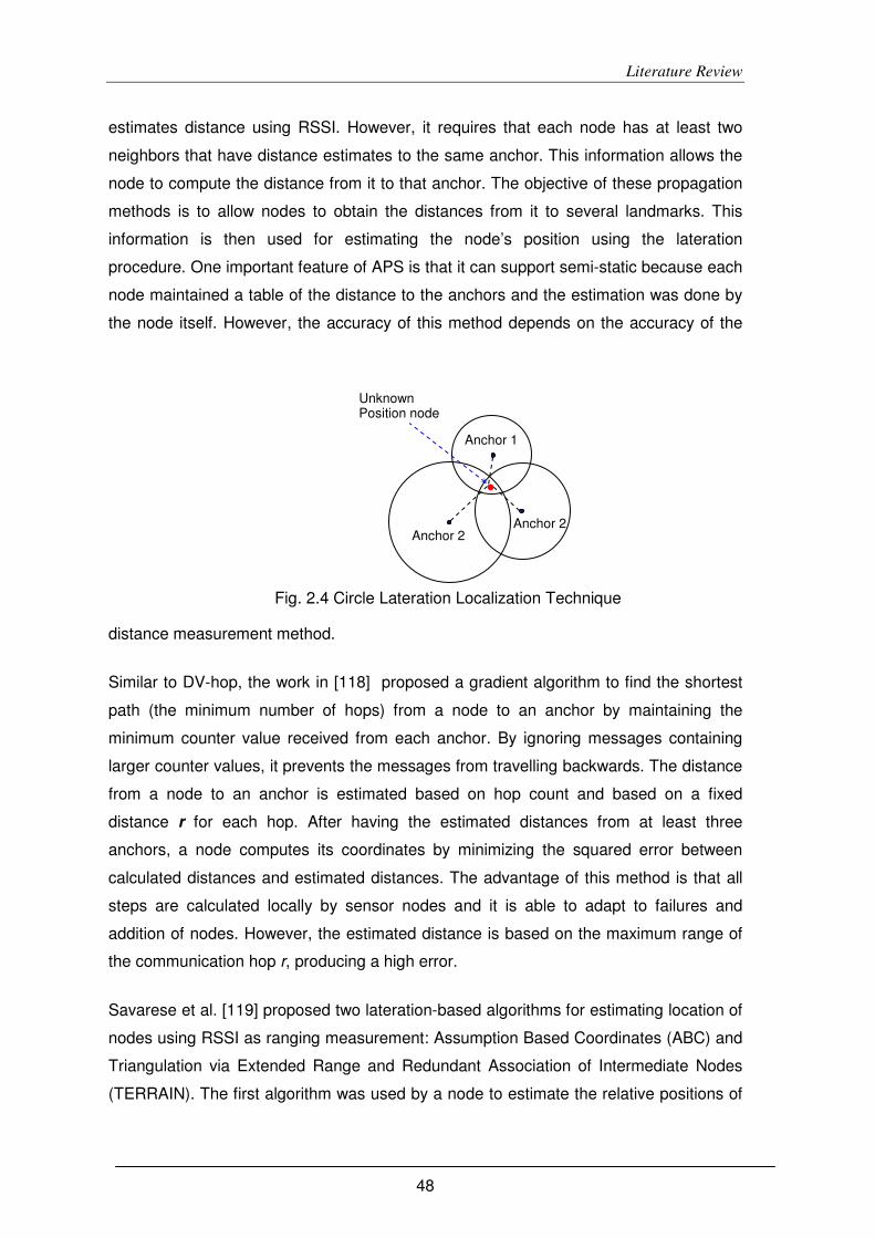
Literature Review
48
estimates distance using RSSI. However, it requires that each node has at least two
neighbors that have distance estimates to the same anchor. This information allows the
node to compute the distance from it to that anchor. The objective of these propagation
methods is to allow nodes to obtain the distances from it to several landmarks. This
information is then used for estimating the node’s position using the lateration
procedure. One important feature of APS is that it can support semi-static because each
node maintained a table of the distance to the anchors and the estimation was done by
the node itself. However, the accuracy of this method depends on the accuracy of the
distance measurement method.
Similar to DV-hop, the work in [118] proposed a gradient algorithm to find the shortest
path (the minimum number of hops) from a node to an anchor by maintaining the
minimum counter value received from each anchor. By ignoring messages containing
larger counter values, it prevents the messages from travelling backwards. The distance
from a node to an anchor is estimated based on hop count and based on a fixed
distance r for each hop. After having the estimated distances from at least three
anchors, a node computes its coordinates by minimizing the squared error between
calculated distances and estimated distances. The advantage of this method is that all
steps are calculated locally by sensor nodes and it is able to adapt to failures and
addition of nodes. However, the estimated distance is based on the maximum range of
the communication hop r, producing a high error.
Savarese et al. [119] proposed two lateration-based algorithms for estimating location of
nodes using RSSI as ranging measurement: Assumption Based Coordinates (ABC) and
Triangulation via Extended Range and Redundant Association of Intermediate Nodes
(TERRAIN). The first algorithm was used by a node to estimate the relative positions of
Anchor 2
Anchor 1
Unknown Position node
Anchor 2
Fig. 2.4 Circle Lateration Localization Technique

Literature Review
49
its neighboring nodes, one at a time, based on the order in which they established the
communication with the node. Assuming that the ABC algorithm starts on the node n0
with the coordinates (0,0,0). For the first few neighbors, it does not have enough
information for forming lateration problem. ABC dealt with this issue as follows. When
the first node communicated with n0, it was considered this node as n1 and its
coordinates would be (r01,0,0). In which r01 is the distance between n0 and n1 based on
the RSSI measurement. The location of the next node (i.e., n2) communicating with n0
was computed using the follow equations [119]:
�� = ���� + ���� + ����2��� ; �� = � ���� − ����; �� = 0
From the node ni (i>=3), its coordinates are estimated using the standard lateration
method (i.e., least square) on the following system of equations [119]:
�� = ���� + ���� + ����2��� ; �� = ���� − � ������ + ����� + ����� + 2������2���� ; �� = ����� − ��� − ���
With ABC the locations of neighbor nodes were relative to that of the estimated node.
Therefore, to determine the global positioning for an ad-hoc sensor network TERRAIN
algorithm [119] was proposed as follows. First, the ABC algorithm was applied at the
anchor nodes. The results computed at the anchor nodes were then forwarded to other
nodes. The unknown nodes waited for the results from at least four independent anchor
nodes to compute its own position using a lateration method. To improve the accuracy,
after these steps the nodes could apply an iterative refinement process [119] which
combines the most recently computed coordinates of its neighboring nodes and the
ranging measurements to these neighbors to recompute its own position.
Collaborative multi-lateration proposed in [120] is another lateration based method that
allows nodes to collaborate with each others to jointly estimate their locations in a multi-
hop ad-hoc sensor network. This method comprises three main phases: (1) formation of
collaborative subtrees, (2) computation of initial estimates, and (3) position refinement.
In the first phase, each unknown position node finds a set of neighboring nodes (at least
three) that satisfy the tentatively unique conditions proposed in [120]. To build the
subtree, each unknown position node tests whether it has at least three neighbors with
tentatively unique positions, i.e., they are anchors or their positions can be estimated
using information from their neighbors. In the second phase, each node estimates its
initial coordinates based on the locations of beacons and the distance measurements to

Literature Review
50
these beacons using the bounding box method proposed in [120]. Finally, the position of
node is refined using Kalman Filter [121], [122] based on the information about the
subtree, its initial position, distance measurements to neighbors and location of
neighbors. Although it was claimed that this method could be implemented in a
distributed mode, it is inefficient or unfeasible to implement the Kalman filter on most of
the current sensor nodes because of the heavy matrix and float number computation.
Proximity Distance Map (PDM) [123] proposed a method to deal with the anisotropic
WSNs in which the nodes were distributed non-uniformly caused by geographic shapes
of the region, different node densities, anisotropic radio patterns, etc. It proposed a
mapping method between the proximity measurement, e.g., RSSI, and a geographic
distance using the truncated singular value decomposition (SVD) pseudo-inverse
technique [29]. To collect the information for this process, PDM employs the method
similar to that of DV-hop [117] to collect the number of hops to the anchors. By applying
the PDM on the hop counts and physical distance between anchors, more accurate
distance estimations for hops are obtained and thus more accuracy in location
estimation. Similar to APS, the node also employs lateration based method to estimate
its position. The drawback of this method is that it requires a high ratio of beacons to
produce the proximity map of anisotropy networks. In addition, SVD has a high
computational complexity O(n3).
2.5.2.1.2 Point-In-Triangle Test
He et al. [124] proposed a distributed localization method based on the Point-In-
Triangle Test (PIT) principle named Approximate PIT (APIT). It consists of four main
steps. First, each node obtains information about the positions of anchors and the signal
strengths to these anchors, and exchanges this information with its neighbors. Then, the
node runs the approximate PIT Test algorithm [124] to determine a set of triangles in
which it resides. In the third step, APIT runs SCAN algorithm [124] to calculate the
intersection of all the triangles determined in step 2. Finally, the coordinates of the node
are the center of gravity of this intersection area. Because APIT runs on every node, it
is totally distributed and it is thus very scalable. However, it requires that the anchors
must have the high power transmitters to reach all the nodes in the network. In addition,
the node density must be high (e.g., each node must have at least 6 neighbors) to
obtain an acceptable accurate rate in the determination of whether a node is inside or
outside a triangle. Furthermore, similar to GPS system, in order for this method to be
applied, each unknown position node must be in range of at least 3 anchors.

Literature Review
51
2.5.2.1.3 Multidimensional Scaling (MDS)-based Methods
Multidimensional Scaling (MDS) is the search for a low dimensional space [125], and it
is often used in reconstructing the maps, i.e., finding relative positions of points in the
maps, given the distances between points. Consequently, MDS can be used in solving
the relative locations of nodes in ad-hoc sensor networks.
One of the localization methods based on MDS is MDS-MAP [126] which accepts as its
input the WSN’s information in form of an undirected graph in which a set of vertices are
the sensor nodes and the edges are measurements between nodes (e.g., signal
strengths or distances). This method consists of three steps. In the first step, the weights
of the edges are assigned based on the input information. If the measurement between
neighboring nodes is the distance then it is also the weight of the corresponding edge,
otherwise, the value one is assigned to all edges. Then, the shortest distances between
all pairs of nodes are computed to construct the distance matrix for MDS. In the second
step, the classical MDS [125] is applied on the distance matrix to construct a 2-D (or 3-
D) relative map of the sensor network. The result from MDS is an arbitrarily rotated and
flipped version of the original layout. Consequently, when there are a number of anchors
exist, step 3 is applied to transform the relative map to an absolute map based on the
position of anchors. This step includes scale, rotation and reflection to minimize the error
of localization. The advantages of MDS-MAP are that it can be applied even if there are
no anchors and the measurement is not the distance but the connectivity information.
A variant version of MDS-MAP to make it work in distributed mode is MDS-MAP(P) [127]
which stands for MDS-MAP using patches of relative maps. MDS-MAP(P) comprises
two main phases: (1) each individual node computes its own local map using its local
information, and (2) the local maps are merged to form a global map. In the first phase,
each node obtains the measurements of its nearby neighbor nodes within Rlm hops (Rlm
was chosen in advanced). Then, it employs the first two steps of MDS-MAP algorithm to
compute its local map. Finally, the node applies the least-square minimization to refine
its local map. In the second phase, local maps are merged to create global map. First,
one node is elected as core map in which the merging process starts. Then, the core
map is grown by merging with the maps of its neighbor nodes. Each time a neighbor
node with maximum number of common nodes is selected. This process is repeated
until the core map covers the entire network. The MDS-MAP(P) [127] also comprises an
optional step to refine the global map by applying least square minimization to the
coordinates produced in previous step. The problem with this method is that it is too
complex for sensor nodes.

Literature Review
52
2.5.2.1.4 Mass-spring based Optimization
Priyantha et al. [128] proposed a distributed localization method based on mass-spring
optimization named anchor-free distributed localization (AFL). In this method each node
is considered as a mass and the edge connects two nodes is considered as the spring
between two masses. The spring is on the rest state when its length is equal to the
measured distance between two nodes; otherwise, there is a force that pulls or pushes
the nodes apart. With this view, localization can be seen as a mass-spring optimal
process. AFL comprise two main phases [128]: (1) generating a fold-free configuration,
and (2) mass-spring optimization. The objectives of the first phase are to avoid folds in
the resulting graph, and to assign the initial coordinates for every node. It starts by
nodes cooperatively electing 5 nodes to become reference nodes using the heuristic
algorithm proposed in [128]. The reference nodes are elected such that four of them are
on the periphery of the graph, and roughly perpendicular pairs; and the fifth node is on
the centre of the graph. Then, every other node, ni, computes its polar coordinates (pi,
θi) as follows:
�� = ℎ�,� ∗ �
�� = tanh�� ℎ�,� − ℎ�,�� ℎ�,� − ℎ ,�� In which, R is the maximum radio range; and hi,j is the hop count from node i to node j
After calculating its polar coordinates, the node periodically broadcasts its position to its
neighbors.
In second phase, every node uses its current coordinates, the coordinates of its
neighbors, the measured distances from it to its neighbors to build the mass-spring
model [128] and runs the optimization process on this model to minimize the errors.
One advantage of this method is that it is anchor-free and it can produce a good network
topology. However, as other anchor-free methods, the resulting graph is usually
translated, rotated or reflected. In addition, it requires distance measurement between
neighboring nodes. Furthermore, it may be too complex for constraint devices.
2.5.2.1.5 Sequential Quadratic Programming
Sequential Quadratic programming (SQP) is a framework for solving the nonlinear
optimization problems directly [129]. It was proposed to solve the localization problem of
static/semi-static WSNs based on the RSSI as shown [130]. The proposed method

Literature Review
53
comprises three stages [130]: (1) RF mapping of the network, (2) Creation of ranging
model, and (3) Centralized localization algorithm. In the first stage, each node
exchanges the short packets at different power levels in order to obtain RSSI values and
then sends them to the centre server for further processing. In the second stage, the
RSSI values obtained in the first phase are used to find the best values for parameters a
and b of the model family !" = # + $"%. In which, Pr is the received power of the signal; r
is the distance, and k can be set to 2, 3 or 4 according to the specific environment.
Finally, the SQP is used to estimate the positions of nodes by minimizing the cost
function proposed in [130], which is the sum of error between the measured and
estimated distance between nodes. This work was validated with a real testbed with
MICAz [47] sensor nodes. However, its drawback is that it requires to create the ranging
model (calibration) for every deployment environment.
2.5.2.1.6 Simulated Annealing Localization
Simulated annealing is inspired by the process of annealing in metallurgy [131], in which
a solid material is heated and then slowly cooled down until it is crystallized. This
process can be simulated to solve the optimal problem. Although it does not guarantee
to find a best solution, it can find a global optimum with a high probability.
Kannan et al. [132] proposed a method based on simulated annealing algorithm to
solve the flip ambiguity problem in the localization problem for WSNs named Simulated
Annealing Localization (SAL). SAL requires m anchor nodes with known locations and
thus the network has n-m unknown location nodes. In addition, before the location
process starts, each non-anchor node is initialized with a random position within the
boundaries of the network. The SAL method consists of two main phases: (1) estimating
the localizable nodes, and (2) refinement of flipped nodes [132]. In the first phase, SAL
employs the simulated annealing algorithm to minimize this cost function [132], which is
the sum of errors of all unknown position nodes. The error at each node is the difference
in the measured and the estimated distances between the node and its one-hop
neighbors. This step results in the positions of all localizable nodes with some flipped
nodes, i.e., nodes with incorrect positions. The second phase is applied by firstly
identifying the nodes whose positions are likely to be flipped and then moving them to
correct positions. To determine whether a node is in the wrong position, SAL compares
the radio range and the Euclidian distance from itself to its non-neighbor nodes. If there
is a radio range greater than the distance, then the node must be in the wrong position.
Literature Review
54
The second phase also uses the simulated annealing algorithm but with a cost function
that takes into account the non-neighbors [132], and it only applies for flipped nodes.
SAL could produce more accurate results by overcoming the local minimum of the
optimal problem. However, it does not guarantee obtaining the optimal answer. In
addition, it requires the distance measurement which is hard to obtain in real
environment. Furthermore, it requires a high node density to obtain a good result.
Otherwise, flip ambiguity cannot be solved because the node is flipped but still maintains
correct neighbors.
2.5.2.1.7 Support Vector Machine
Support Vector Machine (SVM) is a modern approach of learning machine for
classification and regression. The idea of SVM [133] is to find the equations that divide
the feature space into separable hyper-planes with maximum margins around them. The
important feature of SVM is that the decision function is fully specified by a subset of
training samples. This means that after training, the parameters of the model can be
written as subset of training samples, which are so-called support vectors [134]. The
SVM can be used for the localization in ad-hoc WSNs as shown in [135], [136], and
LSVM [137]. The advantage of this method is that it is simpler and with less
computational requirements than other methods. However, it requires a high ratio of
anchors to obtain a good accuracy.
2.5.2.1.8 Hybrid Methods
In [138] authors proposed a localization method named Simple Hybrid Absolute Relative
Positioning (SHARP) which is based on MDS [125] and APS [117]. This method
consists of three phases: (1) selecting preference nodes; (2) localizing reference nodes;
(3) localizing non-reference nodes. First, the reference nodes are chosen randomly or
along outer perimeter of the network using the algorithm that is similar to the algorithm
proposed in AFL [128] but with more reference nodes selected. Then, the MDS [125] is
used to relatively localize the selected reference nodes, using the shortest distances
among reference nodes. The result of this phase is the relative coordinates of the
reference nodes. Finally, the locations of the remaining nodes are estimated using the
reference nodes in second phase as anchors. In the final phase, each node estimates
the distances from itself to the anchors using the DV-distance version of the APS
method [117], and then it computes its own location using the lateration-based method.
Literature Review
55
Another hybrid algorithm is proposed in [139] which combines MDS [125] and PDM
[123] in a phased approach. As most of other methods, this method requires some
nodes with known positions called primary anchors. In the first phase, a subset of
unknown location nodes is elected to become secondary anchors. Then, every node
(including primary anchors) collects the proximity information, e.g., distance or hop
count, to the primary anchors using the similar process proposed in APS [117]. After
having the proximity information to all primary anchors, each secondary anchor
estimates its own position using MDS [125]. In the second phase, PDM [123] is
employed to create the proximity distance mapping among anchors (both primary and
secondary), which is then distributed to all normal nodes. Similar to PDM, each normal
node can then estimate its position using this proximity map and the table of hop count
from itself to anchors. This method reduces the high number of anchors problem in PDM
[123]. However, the introduction of secondary anchors reduces the accuracy comparing
with PDM method.
2.5.2.2 Localization Methods for Controlled Sensor Networks
Because controlled WSNs have been becoming increasing popular, determining the
locations of unknown position (mobile) nodes in this type of networks is more and more
important. This section focuses on the methods that can be used to determine the
positions of sensor nodes in controlled sensor networks.
2.5.2.2.1 Proximity
The proximity localization method is based on the “closest anchor” principle, i.e., the
location of the mobile node is the location of closest anchor based on some
measurement. The measurement can be signal strength or distance. As a result the
closest anchor is the one with the strongest signal strength or shortest distance. Active
Badge [25], [140] was one of the positioning systems that employs this method. The
Active Badge [25], also called the tag, was attached to people, and it emitted a unique
code using infrared (IR) signal every 15 seconds. This information was collected by the
sensors and stored into a central database for use by the location system. The location
system used the position of the sensor which received the last signal from the tag to
infer the tag’s position. Another location system based on this method was Cricket [26],
which based on the distance to infer the closest anchor. In order to produce an accurate
distance estimate, Cricket uses a combination of RF signal and Ultra-sound. In addition,
to overcome the beacon interference problems, a simple algorithm, called MinMode [26],
was proposed to choose the closest beacon. For each beacon, a tag picks the mode of

Literature Review
56
the distance in a time window, and chooses the beacon that has the minimum distance
among all beacons. The advantage of proximity method is that it is very easy to
implement. However, it only provides relative locations such as in which room the mobile
node resides.
2.5.2.2.2 Centroid Method
A simple localization method that uses the measurement from multiple reference points
is centroid algorithm [28]. In this method, the position of a node is determined by the
arithmetic mean of the coordinates of all the beacons that are in range of it. For
example, if a mobile node detects n beacons which are located at positions { Xi=(xi,yi),
i=1,..,n } then its position can be estimated using the equation & = �' ∑ &�. This method is
simple to implement and requires no distance measurement. However, its accuracy is
low. In addition, it produces the same position for the node if it is in the ranges of the
same set of beacons regardless of the measurements.
2.5.2.2.3 Lateration
As presented in the previous section, lateration can be used to estimate the position of a
device by expressing the localization problem as a system of equations. If it is possible
to measure or estimate the distance between the sensor nodes and several anchors
then the localization problem can be expressed as a system of equations of circles or
spheres. However, in case of the differences of time at which the signal arrives at
different anchors obtained, a system of hyperbolas is formed and used to estimate the
position of the transmitter. As shown in Fig. 2.5, the difference between the arrival times
of a signal at two anchors restricts the possible locations of the device to be along a
hyperbola in which two anchors are its foci [107]. By adding a third anchor, two more
hyperbolas are formed. Intersection of two or more hyperbolas defines the possible
location of the device. Similar to circle lateration, this method also faces the problem of
no single point intersection and no intersection of curves. One method to this problem is
to linearize the equations through the use of Taylor-series expansion and to solve it
using the iterative algorithm [141]. Another method is to use the correlation techniques
using the cross-correlation function of the signals [142]. The main disadvantage of
hyperbolic lateration is that it requires that the time of all anchors must be accurately
synchronized. In addition, its accuracy is also severely affected by noise, obstacles, and
NLoS environments.
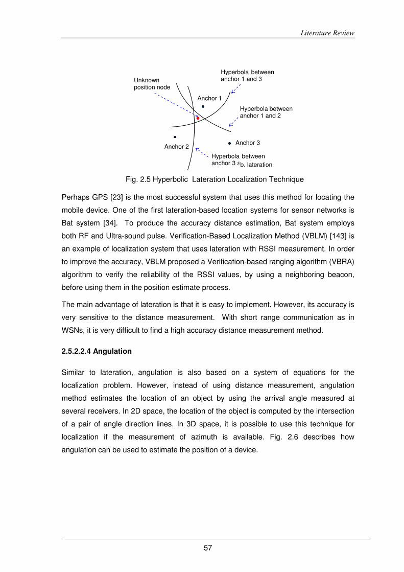
Literature Review
57
Perhaps GPS [23] is the most successful system that uses this method for locating the
mobile device. One of the first lateration-based location systems for sensor networks is
Bat system [34]. To produce the accuracy distance estimation, Bat system employs
both RF and Ultra-sound pulse. Verification-Based Localization Method (VBLM) [143] is
an example of localization system that uses lateration with RSSI measurement. In order
to improve the accuracy, VBLM proposed a Verification-based ranging algorithm (VBRA)
algorithm to verify the reliability of the RSSI values, by using a neighboring beacon,
before using them in the position estimate process.
The main advantage of lateration is that it is easy to implement. However, its accuracy is
very sensitive to the distance measurement. With short range communication as in
WSNs, it is very difficult to find a high accuracy distance measurement method.
2.5.2.2.4 Angulation
Similar to lateration, angulation is also based on a system of equations for the
localization problem. However, instead of using distance measurement, angulation
method estimates the location of an object by using the arrival angle measured at
several receivers. In 2D space, the location of the object is computed by the intersection
of a pair of angle direction lines. In 3D space, it is possible to use this technique for
localization if the measurement of azimuth is available. Fig. 2.6 describes how
angulation can be used to estimate the position of a device.
Anchor 2
Anchor 1
Anchor 3
Unknown position node
Hyperbola between anchor 1 and 3
Hyperbola between anchor 3 and 3
Hyperbola between anchor 1 and 2
Fig. 2.5 Hyperbolic Lateration Localization Technique
b. lateration

Literature Review
58
The advantages of this method are that it does not require time synchronization and
fewer anchors needed as comparing to lateration. However, it requires a more complex
and expensive hardware by using directional antennae [144] or an array of antennae at
the receivers. In addition, it needs a line of sight (LoS) between unknown position node
and the anchors, which are rarely obtained in real environments. Consequently, the
accuracy of this method is severely affected by the shadowing, multipath, obstacles, and
non-LOS environments.
2.5.2.2.5 Kalman filter
Kalman filter [121], [122], [145], [146] is a recursive optimization estimator that is widely
used in almost every fields including localization. It uses the prior knowledge of noise
characteristics to account for and filter out the noises [31]. The Kalman filter processes
all available measurements, regardless of their precision, to estimate the current state of
the variables of interests. To apply the Kalman filter, the real world system must be
described as a set of differential equations, which is the mathematical model for
dynamic systems whose states we want to estimate. It is important to note that the
dynamic system describes the propagation of state mean and error covariance through
time.
The most common way of describing the real world system is in the form of state-space
model [121], [146]:
tanh ��� = �� − ��� − �
θ1
θ2
(x,y)
Anchor 2 (x2,y2)
Anchor 1 (x1,y1)
Unknown position
Anchor 3 (x3,y3)
Fig. 2.6 Angulation Localization Method

Literature Review
59
�) = *� + +
In which:
x is a column vector whose entries are the states of the system;
A the system dynamics matrix;
w is the process noise, which is also expressed as a vector.
There is a process noise matrix Q that is related to the process noise vector and
calculated using the equation , = -[++/]. In addition, the Kalman filter requires that the
measurements are related to the states according to the equation:
1 = 2� + 3.
In which:
z is the measurement vector;
H is the measurement matrix;
v is measurement noise, which is also expressed as a vector.
Similar to process noise, the measurement noise matrix R is related to the measurement
noise vector v according to the equation � = -[33/]. It is important to note that in case
of the measurement equation is non-linear equation then it is called the extended
Kalman Filter [121].
In order to implement the Kalman filter on the computer, the system dynamics must be
discretized. The dynamic system for discrete-time Kalman filter is described as follows
[146, pp. 124-124]:
�4 = 54���4�� + +4��
Then, the discrete form of the Kalman filtering measurement equation becomes:
14 = 24�4 + 34
Kalman filter algorithm consists of two phases: prediction and correction [146, pp. 128-
129]. In the first phase the state of the system is predicted based on the dynamic model
and in the second phase the predicted state is corrected by the data obtained from the
measurements and the observation model. The Kalman filter algorithm tries to minimize
the error covariance of the estimation; therefore, it is an optimal estimator. Fig. 2.7
describes these two phases:

Literature Review
60
In which:
Pk: Covariance of the estimation error.
Kk: Kalman Gain
An important application of Kalman filter in localization is to improve the accuracy of
GPS system as show in [147]. In addition, it is also employed for the localization
problem in WSNs as proposed in [31].
2.5.2.2.6 Pattern Matching-based methods
The pattern matching-based localization methods are also called learning-based or
fingerprinting based methods. The methods in this approach usually consist of two
stages: (1) training stage, and (2) estimating stage. The training stage is often called
offline stage because it is done offline before the location system running to response to
the location request. In order to have the dataset for training the localization algorithm,
the features, e.g., RSSI, of the deployed network are first collected and stored in a
dataset, also called fingerprinting or training dataset. The objective of the training phase
is to build a model or parameters for the localization algorithm. After having a model, the
estimating stage (also called online stage) can be used to estimate position of the
sensor nodes. The common feature collected for localization is RSSI because it is
available in almost every wireless networks. In case of the feature is RSSI, each record
Fig. 2.7 Kalman Filter Algorithm
�64� = *�64��
!4� = *!4��*/ + 7 84 = !4�2/ 2!4�2/ + ����
Prediction Phase:
1. Estimate the next state �64�based on the previous
estimated state �64��:
2. Compute the Covariance and Kalman gain
�64 = �64� + 84 14 − 2�64�� Correction Phase:
1. Estimate the next state base on measurement
2. Compute the error covariance
!4 = !4� + 842!4�

Literature Review
61
of the training dataset consists of the coordinates of the collected position and a list of
RSSI values from nearby anchors. There are several localization algorithms using this
approach including k-Nearest Neighbors (kNN), Probabilistic-based, Support Vector
Machine (SVM) and Artificial Neural Network (ANN).
k-Nearest-Neighbors (kNN)
kNN [148] is a common algorithm in machine learning and data mining for classifying a
test object by finding a group of k objects in the training dataset that are closest (based
on some similarity metric) to it. These k objects in the dataset are called neighbors of the
test object. The resultant class of the test object is the class that predominates in k
involved neighbors. The simplest case of kNN is assigning the test object to the class of
its closest neighbor (i.e., k=1).
kNN can be used to estimate the location of a device by first searching the fingerprint
dataset to find k records, i.e., positions, that have feature(s) most similar to those of the
new observed measurement according to a distance function, e.g., Euclidean distance.
Then, by averaging these k positions, an estimated position of the mobile device is
obtained. The distances between the new observed measurement and k nearest
records can be used as the weights when computing the average and it is called
weighted kNN. The examples of localization systems that employ the kNN include
RADAR [35], LADMARC [37], and MoteTrack [38].
Probabilistic-Based Method
Similar to kNN but instead of using the distance to measure the “similarity” between the
new observed measurement and records in the fingerprinting dataset, the probabilistic-
based method uses the probability theory to determine the similarity between records.
As with kNN, in this method, k records with the highest probability are selected. Then,
the position of the mobile node is the (weighted) average of the coordinates of these k
records.
A common method is to use Bayes rule [149] to calculate the probabilities of matching
between the test object and the records in training dataset. Assuming that the
fingerprinting dataset has n candidate records D = { Li | i=1,...,n }. The class of the new
observed data vector s is determined by the Bayes rule as follows:
Choose class Li if P(Li | s) > P(Lj | s) for i and j=1,..., n and j ≠ i
It is normally assumed that the likelihood of each record in the fingerprinting dataset has
normal or Gaussian distribution in which the mean and standard deviation (SD) of each
anchor at position candidate can be calculated using the measured data. Because the

Literature Review
62
probabilistic-based method takes into account the standard deviation of the measured
feature(s) of each anchor, the accuracy of this method is better than that of kNN. Horus
[39], [150] is an example of the usage of probabilistic-based method for estimating the
mobile nodes in WLAN. In addition, Elnahrawy et al. [151] proposed Area-Based
probability (ABP) to estimate the area in which a mobile node resides for WLAN.
Similarly, [40] is an example of the usage of this method to estimate position of devices
in indoor WSNs.
Support Vector Machines (SVMs)
As discussed in previous section, SVMs, also called kernel machines, are ”maximum
margin methods that allow the model to be written as a sum of the influences of a subset
of training instances” [149]. SVMs can also be used for localization in controlled wireless
network as shown in [44].
Artificial Neural network (ANN)
ANN [152], inspired by the structure and operation of the brain, can also be used to
solve many real world problems in different domains, including pattern recognition and
classification. The neural network structure comprises numerous neurons divided into
multiple layers: one input layer, one output layer and zero or more hidden layers in
between these layers. The neurons are connected to each other and each connection is
assigned a connection weight. The weights of the connections are determined during
the training phase and are used to compute the results when receiving inputs from input
neurons. Different kinds of neural networks are formed by different methods of
connection among neurons. One of the common used neural network structures is feed
forward, i.e., the neurons in one layer only connected to the neurons of the next layer as
described in Fig. 2.8.
The ANN computes the results based on the combination of inputs, the weights of the
connections between neurons and the sigmoid function [152]. For localization, the RSSI
values measured at different positions can be used as inputs for ANN. During the
training phase, the training algorithm uses the coordinates of the measured positions to
calculate the errors. Training neural network can be seen as an optimal problem in
which the errors between the outputs from ANN and the actual values are minimized.
There are a number of approaches for solving this optimal problem including: gradient
descent algorithms, optimization heuristics like simulated annealing or special
optimization techniques like genetic algorithms [152]. After the training phase, the
appropriate weights are obtained and used during the position estimate process.

Literature Review
63
The research on using the ANN for localization in WSNs includes [42], [153], [154]. The
advantage of neural network is that it is very fast to estimate the location (online stage).
However, the training stage takes a very long time and needs experiential or empirical
study to choose the good structure. In addition, it cannot work well in the case the
training dataset has many non-separable records.
From the study in this chapter, we can figure out that the accuracy of the localization
mainly depends on the accuracy and the stability of the type of measurements. In
WSNs, it is a challenge to find such an accurate and stable but cheap measurement
method. As RSSI value is the cheap and available data in WSNs, it is the most common
data used in Localization in WSNs. As a result, the objective of our work is to develop a
scalable localization system target industrial WSNs with an acceptable accuracy.
∫
∫
∫
∫
∫
∫
∫
∫
∫
Input Layer Hidden Layer Output Layer
RSSI_1
RSSI_2
RSSI_3
RSSI_4
x
y
z
Fig. 2.8 An Example of a Neural Network with 3 Layers (4 input neurons, 6 hidden
neurons, 3 output neurons)
Literature Review
64
2.6 Some Related Projects
This section reviews some projects that are related to the work done in this thesis.
One of the project that is closely related to the work in chapter three of this thesis is
GINSENG project [155]. The aim of this project is to develop a performance-controlled
Wireless Sensor Network that guarantees reliable and timely data delivery. The targets
of this project are critical environments such as the oil refinery in which the time
response, packet loss and reliability are bounded by some constraints.
WSN-DPCM project [156] is a international project that develops toolset for developing,
planning, commissioning and maintaining large-scale WSNs. It includes reusable
middleware for heterogeneous hardware platforms. In addition, it also has tools for
assisting the planning the sensor network before deployment. This helps to reduce the
time of trial-and-error iterations. Furthermore, it also consists of the integration toolset to
seamlessly handle the information flow between tools.
CodeBlude [157] is a project which explored medical sensors as well as software for
wireless medical devices. One of the areas of this project was 3D location tracking using
radio signal information. The MoteTrack location system [38] is one of the outcomes of
this project.
Smart Monitoring of Historic Structures [158] is a project which uses sensor network to
monitor ambient conditions of the historic structure such as temperature, humidity, air
velocity, vibration etc. This helps the owners and professional to identify the threats to
produce recommendations for action.
EMMON - EMbedded MONitoring [159] is another project for monitoring the physical
properties of specific geographical areas. One of its objectives is to improve reliability
and fault tolerance mechanisms in WSN. In addition, it also target at the middleware for
end-users to monitor and control WSN.

Literature Review
65
2.7 Summary
This chapter presented an overview of WSN, its challenges and requirements. In
addition, it reviewed the research on the coexistence, integration, and localization
problems.
It is important to note that the MAC protocols could provide some level of reliability for
communication in WSNs. However, it usually has the problem in the noisy and
interference environments in which there are other wireless networks or devices
operating on the same frequency band. Cognitive radio may be a potential technique for
dealing with the interference and polluted environments. However, it is too complicated
for WSNs and may not work well in case of the noise and interferences change with
time. Consequently, it is important to have an appropriate mechanism to provide a
reliable communication for WSNs operating with environments.
Implementing TCP/IP protocol stack and web services on sensor nodes realizes the
vision of IoT. However, it is not the solution for all WSNs. In fact, it is not appropriate for
many types of current WSNs. As a consequence, gateway-based approach is still a
common method for integrating WSNs with external environments in the foreseeable
future. The primary advantage of gateway-based approach is that it hides the details of
sensor networks from external environments. In addition, the developers can freely
choose protocols and applications for sensor networks. More importantly, by exposing
the data and functionality of a WSN as web services, WSNs can be treated as traditional
networks. However, the problem with current gateway-based approach is that the
gateway or proxy is application-specific, i.e., it has to be modified or reprogrammed
when using for other sensor network or adding new applications to current network.
Although there is a large volume of publish studies on localization for WSNs, it is still a
hard problem in terms of accuracy. The main reason behind this is that is difficult to
have an accurate, reliable, and low-cost measurement technique for WSNs. In addition,
the scalability of localization system is also a concern because the sensor network
usually comprises a large number of nodes and is deployed in a large region.
Consequently, it is necessary to have a scalable, low cost and near real-time localization
system for controlled WSNs that can produce an acceptable accuracy.
In summary, the work in this thesis tackles three main problems for WSNs: (1) reliable
communication, (2) integration, and (3) localization.

Quality of Channels of IEEE 802.15.4 Compliant Sensor Networks and DynMAC
66
3 Quality of Channels of IEEE 802.15.4 Compliant Sensor
Networks and Dynamic MAC
Summary
3.1 Introduction
3.2 Quality of Channels of IEEE 802.15.4 Compliant Sensor Networks
3.3 Dynamic Medium Access Control (DynMAC)
3.4 Experiment Results
3.5 Conclusion
ne of the crucial requirements of WSNs is to maintain its operation
uninterruptedly for a long duration. Besides the energy, routing and security,
there are other factors that might affect the reliability of a sensor network such
as noise and interference at the deployment environment. The effects of these factors
are different from place to place and from time to time. In addition, their effects might
also be different on different channels of a standard compliant device. This chapter
presents a study of quality of channels of IEEE 802.15.4 compliant sensor networks at
different environments. In addition, it also presents a proposed solution for providing the
reliable communication for sensor networks in noisy and interference environments.
More importantly, the proposed solution includes mechanisms to deal with the noise and
interference that are changeable with time.
O

Quality of Channels of IEEE 802.15.4 Compliant Sensor Networks and DynMAC
67
3.1 Introduction
WSN is different from other types of networks in that the end users seldom interact
directly with the nodes, but mainly with the applications at the control centre. The reason
behind this is that the sensor nodes do not have a user interface. In addition, they may
be deployed into areas to which the users may not have access. Moreover, there could
be so many nodes that users cannot deal with them individually. Therefore, energy
efficiency and high reliability are the main concerns when designing and deploying
sensor networks. This study focuses on the latter requirement, i.e., reliability for sensor
networks, without neglecting the former requirement.
There are several factors that affect the reliable communication of WSNs including the
noise and interference caused by the other wireless networks, e.g., Wi-fi, Bluetooth,
cordless phone, machinery and other devices. Because of the limitations of sensor
nodes, their radios are more susceptible to noise and interference than those of other
wireless technologies. Consequently, the effects of these factors on the quality and
stability of the sensor networks are even more severe.
Each wireless communication standard usually supports a set of discrete channels,
allowing a wireless network to utilize a single channel or a subset of these channels.
Therefore, multiple wireless networks of the same standard or different standards of the
same frequency band can coexist in the same area by using different channels.
However, several questions arise for this situation. First, how to determine which
channels are not occupied? This means that how to determine unused channels in an
area in which other wireless networks exist? In addition, how to determine the effects of
the above-mentioned factors on different channels of a standard compliant device?
Moreover, how to deal with the noise and interferences in case of the new wireless
networks or other devices are added. In fact, all of these questions are related to the
problem of dynamically selecting the most appropriate channels during the operation for
a sensor network. This chapter presents a study and a solution for this problem. In
particular, it presents the results of a study about the quality of different channels of
IEEE 802.15.4 compliant sensor networks in several environments. More importantly, it
details the proposed MAC protocol to deal with the noise and interference that are
changeable with time, allowing WSNs to coexist with other wireless networks and to
work smoothly in noisy environments.

Quality of Channels of IEEE 802.15.4 Compliant Sensor Networks and DynMAC
68
3.2 An Empirical Study of Quality of Channels of IEEE 802.15.4
Compliant Sensor Networks
A defining characteristic of wireless communication is that its signal strength varies over
time, location, and frequency [160]. In addition, the radio frequency (RF) signal is
influenced by multiple factors such as interference, noise, multi-path, shadowing, etc.
These factors affect the error rate, delay, and the stability of the signal strength in the
WSNs and thus their reliability and the quality of service. Furthermore, most wireless
networks, including WSNs, are deployed using the default or a random channel, thus
making the interference problem worse.
In this section, we present the experimental studies of the quality of channels of IEEE
802.15.4 compliant sensor networks in ISM band. We are particularly interested in the
study of quality of wireless sensor networks in differences environments both academic
and industrial as most current studies and experiments were done in purely academic or
laboratory. We conducted experiments at several different locations including an oil
refinery where we implemented WSNs as the case study in the context of the FP7
GINSENG project [155]. Our study shows that it is very difficult to predict the quality and
reliability of the different channels of a sensor network at because the environment
conditions greatly influence the network performance. Consequently, empirical approach
is a suitable method for choosing the appropriate channels to deploy WSNs in noisy and
interference environments.
3.2.1 IEEE 802.15.4 Standard
IEEE 802.15.4 [48] was intended to be the key enabler for low complexity, ultra low
power consumption, and low data rate wireless connectivity among inexpensive fixed,
portable and moving devices. In fact, it was proposed as a standard for WSNs. IEEE
802.15.4 based networks can utilize three Radio Frequency (RF) bands: 868–868.6;
902–928 and 2400–2483.5 MHz; these are referred to as 868, 915, and 2450 MHz
bands, respectively. The 2450 MHz band is commonly known as the Industrial, Scientific
and Medical (ISM) band. The frequency bands, modulation techniques, and data rates
of IEEE 802.15.4 are described in Table 3.1. The frequency bands 868 and 915 MHz
can utilize Binary Phase Shift Keying (BPSK), Amplitude Shift Keying (ASK), or
Orthogonal Quadrature Phase Shift Keying (O-QPSK) modulation while the ISM bands
(2450 MHz) only use O-QPSK modulation. This standard divides the available spectrum
in the three bands into a total of 27 channels as follows [48]:

Quality of Channels of IEEE 802.15.4 Compliant Sensor Networks and DynMAC
69
• channel k = 0, at the frequency of 868.3 MHz
• channels k = 1…10, at frequencies 906 + 2(k − 1) MHz
• channels k = 11…26 in the ISM band, at frequencies 2405 + 5(k − 11) MHz.
Channel allocation in the ISM band is illustrated in Fig. 3.1.
The PHY protocol of IEEE 802.15.4 can handle packets with the payload up to 127
bytes each. IEEE 802.15.4 networks support two main types of topologies: peer-to-peer
and star. These networks can operate in beacon-enabled mode, which utilizes the
slotted CSMA/CA access mechanism, or beaconless mode, which employs the
unslotted CSMA/CA. In the beacon-enabled mode, contention-free access can be
provided by the coordinator, i.e., the nodes can request a guaranteed time slot (GTS) of
appropriate duration and the coordinator decides whether to accept or reject the request
[48], [161].
As the ISM band is the common used band and supported by most sensor vendors, we
did our experiments on sensor networks operating on the channels of this band.
Fig. 3.1 Interference Between IEEE 802.15.4 and IEEE 802.11g
PHY (MHz) Frenquency band (MHz)
Modulation Bit rate (kb/s) Symbol rate (ksymbols/s)
868/915 868–868.6 902–928
BPSK BPSK
20 40
20 40
868/915 868–868.6 902–928
ASK ASK
250 250
12.5 50
868/915 868–868.6 902–928
O-QPSK O-QPSK
100 250
50 62.5
2450 2400–2483.5 O-QPSK 250 62.5
Table 3.1 Frenquency Bands and Data Rates of IEEE 802.15.4

Quality of Channels of IEEE 802.15.4 Compliant Sensor Networks and DynMAC
70
Because ISM band is also used by other wireless network protocols (e.g., Bluetooth,
IEEE 802.11b,g,n), IEEE 802.15.4 based sensor networks frequently coexist with other
wireless networks, affecting each others’ quality and reliability. However, the effects of
this interference may not be the same on all channels. We are experiencing this problem
in the context of the FP7 European Project GINSENG [155] in which a real WSN was
implemented at Galp Energias refinery, Portugal. While at first the sensor network was
configured to operate on the default channel (e.g., channel 26), we soon discovered that
the hazardous refinery environment (containing machineries, pumps, tubes, various
metallic structures, etc) greatly influenced the networks performance, which was very
good in our early laboratory prototypes. This issue brought several questions to our
attention: do the different channels of IEEE 802.15.4 compliant WSNs have the same
quality? How are they affected by factors such as interference and noise? How is the
quality of channels of WSNs in different environments? In order to find the answers to
these questions, we decided to conduct an empirical study about the characteristics of
the channels of IEEE 802.15.4 compliant WSNs in different environments.
The main contribution of this work is to propose an experimental procedure study the
characteristics of different channels of IEEE 802.15.4 compliant sensor networks. In
addition, different metrics (RSSI, loss rate, delay) of the different channels of IEEE
802.15.4 compliant sensor network in different environments were measured and
analyzed. The results of this study showed that the performance and reliability of the
IEEE 802.15.4 channels are channel-specific and location-dependent. As a matter of
fact, it is necessary to do the empirical study of the deployed environment before
selecting a channel or channels to use for a sensor network. As far as we know this is
the first time that WSNs are being used in critical environments like refineries. From the
scientific point of view this is very important because refineries represent one of the
most critical industrial environments.
3.2.2 Related Work
The major studies in wireless communication are about radio propagation modeling
[162], [163], which models the behavior of radio wave propagation signals in different
environments. These models help to predict the quality and reliability of wireless
networks in different environments. However, it is required to have the knowledge to
choose the right model for a specific environment. Therefore, the accuracy of these
methods is limited since different models give different results. In addition, in some
environments, it is very difficult to find a suitable propagation model.

Quality of Channels of IEEE 802.15.4 Compliant Sensor Networks and DynMAC
71
In wireless communication, the Received Signal Strength Indication (RSSI) is the
measurement of the power level of the received signal. In addition, in [164] RSSI and
Link Quality Indicator (LQI) were used to study the spatial and temporal characteristics
of IEEE 802.15.4-compliant sensor network in a specific environment. In this study, the
RSSI and LQI were measured at different locations in a specific room. The measured
information could be used to predict the performance at any location in the room. A
similar work was done by Doherty et al. [165] which studied quality and stability of
different channels and of different channel paths. However, they studied the
characteristics of channels on only one environment (i.e., the printing factory in
Berkeley, California) and did not present a comparison with other environments with
different conditions. In addition, in this study the characteristics of channels could be
affected by internal interference (i.e., other sensor nodes in the same network).
3.2.3 Experimental Environments
In our experiments we used TelosB sensor nodes [47], Contiki Operating System [95],
and X-MAC protocol [62], a duty-cycle (i.e., it uses awake, sleep intervals) low power
MAC protocol for wireless sensor networks. It reduces latency and energy consumption
by letting the senders use a short preamble with target address. When a receiver wakes
up and receives a preamble having a target address equal to its address, the receiver
will send an early ACK to inform the sender that it is ready to accept a packet. The short
preamble saves energy at the transmitter and receiver with low latency. X-MAC protocol
does not support retransmissions in case of packet errors (e.g., by collisions or
interferences). In our experiments, the X-MAC was set to turn on the radio to check the
channel at the rate of 8 Hertz (i.e., 125 ms). The transmitted power in the experiments
was set to 0 dBm (i.e., 1 milliwatt).
In order to study the characteristics of the channels, different environments have been
selected to perform the experiments. The first one was a room without interferences
from other ISM wireless networks. The second environment was an open space also
without the presence of any other ISM wireless networks. These two environments were
considered “clean environments” because there were no interferences from other
wireless networks, no obstacles, and no obvious noise sources. The third environment
was our laboratory at the Department of Informatics Engineering of the University of
Coimbra. This is a noisy and interference environment because there exist several IEEE
802.11g wireless networks that operate on the channels 1, 6 and 11. The interference
between these wireless networks and the IEEE 802.15.4 standard is shown in Fig. 3.1.

Quality of Channels of IEEE 802.15.4 Compliant Sensor Networks and DynMAC
72
The final location is an industrial environment at the Sines refinery, Galp Energia,
Portugal. Although there are no other wireless networks that interfere with the IEEE
802.15.4 within the refinery, there is a considerable amount of noise caused by several
types of machines, pumps, etc working 24 hours a day.
3.2.4 Study Method
The following data was collected to study the characteristics of different channels of the
IEEE 802.15.4 based WSNs:
• Channel number
• Message sequence number
• Received Signal Strength Indication (RSSI) of each packet
• Delay time (the time it takes to transmit a packet from sender to receiver)
In order to avoid internal interference among sensor nodes, a simple sensor network
with two motes was setup to gather the necessary data. One mote acted as base station
and was connected to a computer to collect and record the data for post-processing.
This mote also controlled which channel the sensor network should operate on and
when it would switch to a different channel. The workflow of the base station and that of
the normal node are described in Fig. 3.2a and b, respectively.
The base station starts to operate on a predefined channel, which is set manually in the
code or at installation time. As described in Fig. 3.2a, after setting the start channel, it
initializes two timers. The first one, which is fired periodically every tr time units, is used
to send request messages. These messages are used to collect the metrics, e.g., RSSI,
delay and loss rate, for evaluating the characteristics of the channels. The second timer,
which is fired periodically every tsc time units, is used to control the operating channel,
i.e., when the network should switch to a different channel. When the tsc event occurs
the base station calculates the new channel on which the sensor network should
operate. It then broadcasts the channel switching messages three times to insure that all
nodes receive the request. It is important to note that before sending the channel
switching messages the base station stops the timer tr. In order to make the system
work smoothly, after broadcast the switching channel messages the base station waits
for a while (e.g., 15 seconds) before switching to the new channel. After switching to
new channel, the base station restarts its tr timer to continue the measuring process. In
our tests, tsc and tr were set to 5 minutes and one second, respectively.

Quality of Channels of IEEE 802.15.4 Compliant Sensor Networks and DynMAC
73
Like the base station, all the other nodes in a sensor network are set to start with a
predefined channel. The predefined channel on the nodes and base station must always
be the same. After booting, the nodes start listening for the messages and other events
on this pre-defined wireless channel. When receiving a request message from the base
station, the node will get the RSSI of that message and send this information to the base
station. If it receives a channel switching message, it will switch to the indicated channel,
and start to listen on this new channel. This process is repeated indefinitely.
Although the communication between two motes cannot represent the traffic model of a
typical real multi-node WSN, it is enough to study the characteristics of channels of
IEEE 802.15.4 based sensor networks. However, we also did some experiments with a
multi-node sensor network (1 base station and 3 normal nodes) to evaluate how the
internal interference affects the performance of the sensor network.
Because the main objective of the experiments is to study the characteristics of
channels of the IEEE 802.15.4 based sensor networks, the uniform traffic model was
used. Although it is unrealistic traffic model, uniform traffic model is sufficient for
studying the metrics and for understanding the characteristics of IEEE 802.15.4 based
sensor networks. In this simple sensor network, the base station broadcasts a request
message to the other node every one second (this schedule can be changed), which
Type of Event
Channel switching
start
Setting the start channel
Listen for messages and events
Return RSSI to Base Station
Switching to new channel
End
Request message Stop
Type of Event
Stop
start
- Setting the start channel - Initializing the timer tr - Initializing the timer tsc
Broadcast request message
Calculating new channel
- Stop tr timer - Broadcast channel
switching message (3 times)
- Wait for t seconds
- Switch channel - Restart tr timer
End
tr event tsc event
b. The workflow of the normal node
Fig. 3.2 The Workflow of the Nodes in the Experimental Network
a. The workflow of the Base Station

Quality of Channels of IEEE 802.15.4 Compliant Sensor Networks and DynMAC
74
includes the message sequence number for tracing and computing the loss rate. In
order to calculate the round-trip time between the base station and the other node, the
base station records both the time when it sends a request message as well as the time
when it receives the returned message.
3.2.5 Experimental Results
3.2.5.1 The Characteristics of Channels in Clean Environments
In the first two experiments we intended to study the characteristics of the IEEE
802.15.4 based sensor networks in a clean environment, i.e., no interference from other
ISM wireless network sources, no obvious noise source and no obstacles. For the
indoor environment, we did the experiments for 20 hours. As shown in Fig. 3.3a, the
average received signal strength of channels varies similar to a sine line. It begins with a
low RSSI then alternatively increases and decreases. As we can see, the RSSI of
channels 11 and 18 were lower than the rest. In addition, some middle channels (e.g.,
17, 18 and 19) have outliers with rather low signal strength (< −75 dBm) that might affect
the loss rate. As shown in Fig. 3.3b, some channels have a higher packet loss rate than
the others, especially channel 17.
The Fig. 3.3c presents the delay of transmission on each channel. Although the average
delay was not much different among channels, some channels had outliers, which may
be caused by collisions, and therefore packets lost. Although the network is simple and
only comprises two nodes, packet collisions still occur because the communication
between two nodes is two-way. When a packet was delayed at the received node, the
response packet sent from the received node could probably collide with a new packet
sent by the base station. The delay was caused by the processing or by the duty cycled
of X-MAC [62] protocol. In addition, the large packet delay could also be caused by the
quality of the antenna. As simplistic design philosophy and the constraints of sensor
nodes, its radio often has minimum complexity (quality). Moreover, the antennae of
sensor nodes are anisotropic and RSS of radio is very susceptible to the environment: a
small change in position or direction of the sensor node could result in a large variance
in RSSI values. These factors lead to the instability of sensor radio. As we see in Fig.
3.3, the channels with the highest loss rate usually have the lowest signal strength with
a larger variation (i.e., standard deviations) and/or outliers in signal strength or delay.
For example, in case of channel 17, its signal strength had many outliers with very low
value as well as various outliers in delay. Consequently, its loss rate was very high.
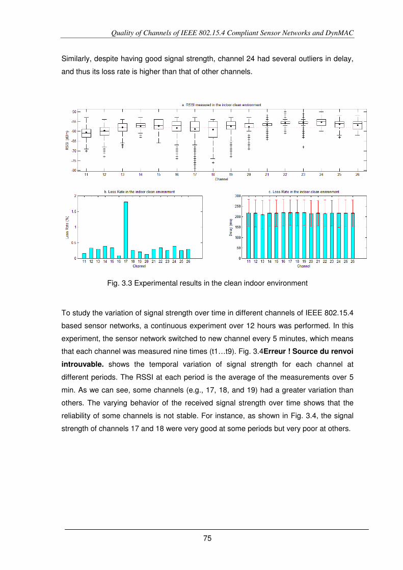
Quality of Channels of IEEE 802.15.4 Compliant Sensor Networks and DynMAC
75
Similarly, despite having good signal strength, channel 24 had several outliers in delay,
and thus its loss rate is higher than that of other channels.
Fig. 3.3 Experimental results in the clean indoor environment
To study the variation of signal strength over time in different channels of IEEE 802.15.4
based sensor networks, a continuous experiment over 12 hours was performed. In this
experiment, the sensor network switched to new channel every 5 minutes, which means
that each channel was measured nine times (t1…t9). Fig. 3.4Erreur ! Source du renvoi
introuvable. shows the temporal variation of signal strength for each channel at
different periods. The RSSI at each period is the average of the measurements over 5
min. As we can see, some channels (e.g., 17, 18, and 19) had a greater variation than
others. The varying behavior of the received signal strength over time shows that the
reliability of some channels is not stable. For instance, as shown in Fig. 3.4, the signal
strength of channels 17 and 18 were very good at some periods but very poor at others.

Quality of Channels of IEEE 802.15.4 Compliant Sensor Networks and DynMAC
76
In addition to the indoor clean environment, we also did some experiments with the
outdoor clean environment. Similar to the indoor clean environment, some channels
(e.g., 11, 12, 13, and 14) had lower RSSI values than others as depicted Fig. 3.5a. In
addition, the channels with low RSSI usually have more packet loss, taking as an
example the channels 11, 13, and 15 as shown Fig. 3.5Erreur ! Source du renvoi
introuvable.b. The average delays are not so different between channels, but similar to
the indoor clean environment case, i.e., the channels with high packet loss have outliers
in delays.
Fig. 3.5 Measurement results in the clean outdoor environment
Fig. 3.4 The Variability of the RSSI with Time in Clean Indoor Environment

Quality of Channels of IEEE 802.15.4 Compliant Sensor Networks and DynMAC
77
3.2.5.2 Effects of Interference on IEEE 802.15.4 based Sensor Networks.
To study how the interferences from other ISM wireless networks affect the IEEE
802.15.4 based sensor networks, we did numerous experiments at our laboratory at the
University of Coimbra. Several IEEE 802.11g wireless networks operating on channel 1,
6, and 11 present in the laboratory building. The interference between these wireless
networks and an IEEE 802.15.4 based network is described in Fig. 3.1. From this figure,
we can guess that the channels 15, 20, 25, and 26 potentially have better quality (signal
strength, loss rate, delay, etc) and reliability than the others. The results of our
experiments over 10 continuous hours were depicted in Fig. 3.6.
As shown in Fig. 3.6a, besides the non-interfered channels, some other channels also
have acceptable quality and reliability such as 16, 17, 19 and 21. We can also see that
the best channels (high signal strength, less loss rate, and short delay time) are not the
non-interfered ones. In terms of loss rate channel 16 and 19 were the ones with the
greatest performance. It is important to note that the results depicted in Fig. 3.6 are
similar to the clean environments in which some initial channels (e.g., 11, 12 and 13) are
worse concerning signal quality and loss rate.
Fig. 3.6 Experimental Results in an Interference Environment

Quality of Channels of IEEE 802.15.4 Compliant Sensor Networks and DynMAC
78
3.2.5.3 IEEE 802.15.4 Channel Quality in Noisy Environment
The final environment where we did the experiments was the Sines Refinery, Galp
Energia, Portugal. This is the environment in which the real sensor networks have been
deployed, as part of GINSENG project [155], for monitoring and controlling the physical
environment. As shown in Fig. 3.7, the results are not easy to predict as in case of pure
interference environment presented in previous section. Although the RSSI of the first
channel (channel 11) is better than in the other channels, in accordance to environments
previously studied, its loss rate is high due to some sporadic conditions. In addition, the
large RSSI variation of this channel is also leading to instable channel. From the results
of Fig. 3.7a, we also see that channels 16, 18, 19, and 20 are more stable than the
others since their signal strength is less spread (less variance). Channel 23 is the worst
in terms of both signal strength and loss rate. A more important point in the result of this
experiment is that although there is no interference from other wireless networks, the
loss rate of all channels are very high. The reason behind this is the noise caused by the
infrastructure of the refinery, e.g., machinery, bumps, etc.
Fig. 3.7 Experimental Results in an Oil Refinery

Quality of Channels of IEEE 802.15.4 Compliant Sensor Networks and DynMAC
79
3.2.5.4 Characteristics of Channels of IEEE 802.15.4 in Multi-motes Sensor
Network
To see how the internal interference influences the characteristics of IEEE 802.15.4
based sensor network, we did several experiments with a four-mote sensor network in
three different environments. The Fig. 3.8 shows the results of these experiments. As
we can see from this figure the internal interference significantly affects the quality of
channels because the increasing in the number of sensors causes the collisions
increasing, therefore, influencing the RSS, loss rate, etc. However, the effect was not
the same in all channels. In addition, as in case of simple 2 mote network, the quality of
channels also depends on the environments.
As shown in Fig. 3.8, a channel is good in one environment may become worse in
another. As an example, the loss rate of channel 19 indoor clean environment is good
but it become worse in the outdoor clean environment. In terms of RSSI, channels 15,
a. RSSI measurement on a multi-mote sensor network b. Delay on a multi-mote sensor network
c. Loss Rate on a multi-mote sensor network
Fig. 3.8 Experimental Results of a four Mote Sensor Network

Quality of Channels of IEEE 802.15.4 Compliant Sensor Networks and DynMAC
80
22, and 23 are stable than the others. As for delays, channels 13, 14, 17, 18, 20, and 21
are better. Concerning loss rate, channel 14, 22 and 23 are better.
3.2.6 Discussion
From the experimental results over the different environments we could make several
remarks about the characteristics of channels in the IEEE 802.15.4 based sensor
networks.
- The quality and reliability of sensor networks are affected by multiple factors
including noise, interference and obstacle. In addition, these effects are not the
same on different channels.
- The characteristics of channels also depend on the deployment environment. In
clean environments or the ones with the presence of known interference
sources, by using the knowledge of present wireless networks we could choose
a-priory the appropriate channels for deploying a wireless sensor network.
However, in environments with noisy sources, predicting the best channels is
very difficult without an empirical study.
- The quality of signal strengths of a channel also varies with time. In some cases,
a channel is good at a time but very bad at some others.
- The signal strength has significant impact on the performance and on the
reliability of the wireless communication.
- In WSNs, because of the limited battery of sensor nodes, it is required that the
radios transmit at very low power. Therefore, the effects of noise, interference,
obstacles, etc on the WSNs are more severe than on other wireless networks.
- There may be other hidden factors that affect the quality and reliability of
different channels of a sensor device.
From these studies, we recognized that the noise, interference and other factors
significantly affect the performance of IEEE 802.15.4 compliant sensor networks. More
important, the effects of these factors are not the same on different channels.
Consequently, it is very difficult to predict the quality of different channels of a sensor
network at the deployment environment. From the results of our experiments, we can
conclude that when deploying a wireless network, especially sensor networks in noisy
and interference environments, it is necessary to have an experimental evaluation
phase, where the behavior of different wireless channels in the deployment environment
is analyzed in order to select the most suitable one(s). Another important point to note is
that the conditions of deployment environment, e.g., noise, interference, can be changed
Quality of Channels of IEEE 802.15.4 Compliant Sensor Networks and DynMAC
81
during the operation of WSNs. Therefore, it is important to have mechanisms to deal
with such changeable environments. The next section presents our proposed solution to
this problem.
3.3 Dynamic Medium Access Control protocol (DynMAC)
Wireless communication is very useful and flexible but, on the other hand, it is also
susceptible to noise, interference, multi-path, obstacles, among other problems. As the
wireless communication presents almost everywhere, the problems of interference,
spectrum pollution, and network coexistence have been increasing. Thus, this leads to
several challenges to assure the quality and reliability of the wireless network in such
conditions, especially for industrial and critical environments.
3.3.1 Context
The demand for ubiquitous and wireless devices has grown exponentially in recent
years, as more and more applications were created. However, the extensive use of
these devices in the same location causes problems because many of them use
the same unlicensed radio spectrum known as ISM bands. In addition, ISM bands are
also used by other devices such as microwave ovens, remote controls, cordless phones,
Bluetooth communications, Hi-Fi and video systems. Although most of these devices
have small ranges and use signals with low amplitude, their interference and noise in
the ISM spectrum is not negligible.
In industrial scenarios, however, the effects induced by common ubiquitous mobile
devices are lower due to the strict control typical of these environments. Nevertheless,
the interference problem still arises because of the multiple wireless devices working in
the ISM spectrum, such as monitoring and actuator devices. In addition, as industrial
applications demand very strict requirements in regards to packet delay and packet loss,
the interference may lower the expected quality of service (QoS). Because WSNs are
increasingly used to replace old cabled monitoring and actuator systems, the
coexistence of different wireless networks and devices may result in several problems
including communication failures or inadmissible response time. These problems are
especially serious in critical and industrial systems.
Because IEEE 802.15.4 based WSNs operate on the same frequency band as that of
WLAN (IEEE 802.11 b/g/n), the most common wireless communication existing almost
everywhere, and the interference will occur if they are deployed in the same area. As

Quality of Channels of IEEE 802.15.4 Compliant Sensor Networks and DynMAC
82
shown in Fig. 3.1, these two standards divide frequency band into channels of 5MHz
and 22MHz respectively and they overlap in almost all extension of the spectrum. This
demonstrates that the frequency spectrum in the ISM bands may become overloaded
even for the WSNs. Several studies were done to understand how the interference from
these two types of networks affects each other.
The studies in [166] showed that at some places the 2400 MHz frequency spectrum, a
frequency used by several wireless networks, had an occupation of 90%. In addition,
Zhou et al. [86] predicted that the growth of wireless communication networks using the
ISM spectrum would suffer overlapping problems. The coexistence of different networks
and devices that operate in the same frequency, or in adjacent frequencies, may
lead to harmful interference, limiting the capabilities of the applications and, in some
cases, resulting in the complete shutdown of those networks [167]. The study in [1]
showed that with the interference of IEEE 802.11 network the Packet Error Rate (PER)
of IEEE 802.15.4 can be up to 95% when the interferer is in the distance of 1.5 meters.
Inversely, the throughput of IEEE 802.11network can be reduced up to 30% when the
IEEE 802.15.4 in a short distance [2]. In addition, Toscano and Bello [81], [82] figured
out that even in networks environments only consisting of WSNs, the interference still
exists. By testing IEEE 802.15.4 networks their results showed that interference
depends on the transmission power, on the distance between nodes and on the duty-
cycle. Our study presented in previous section showed that the quality of different
channels of IEEE 802.15.4 compliant WSNs varies from place to place. In addition, in
the same place the quality of channels also varies from time to time. Moreover, the
effects of noise and interference are very difficult to predict especially in noisy
environment such as refinery. Consequently, it is necessary to have mechanisms for
WSNs to operate in the interference and noisy environments.
3.3.2 Related Work
WSNs deployed in industrial and critical environments require strict performance control
especially in regards to packet delay and loss. Most of the problems arise during packet
transmission and relate to the transmission medium (e.g. signal path-loss, noise and
interference) and poor hardware. Controlling the transmission power, improving the
antennas, and carefully placing transmitters and receivers can partly reduce the effects
of noise and path-loss. Interference occurs due to the existence of more than one
network or by the spectral spread in some wireless standards. Solutions to mitigate or
avoid interference include selective licensing of spectrum by area, use of hardware

Quality of Channels of IEEE 802.15.4 Compliant Sensor Networks and DynMAC
83
standards and use of signal coding. However, in a non-licensed frequency spectrum
such as the ISM, there is no guarantee of noninterference. Consequently, in this
frequency bands, any interference from ISM devices must be tolerated as unlicensed
operations are typically permitted to use these bands.
Two different types of interference in WSNs are co-channel and adjacent channel. Co-
channel interference is defined as the use of the same frequency by more than one
network or device in the same area [83]. This interference cannot be solved with the
increase of the signal power, as that would increase the interference and the
communication problems in any neighbor networks. Adjacent channel interference
occurs when consecutive channels are used by different devices in the same area,
which leads to the degradation of both signals. To avoid this type of interference,
channels in a wireless standard are separated in frequency. However, that may not be
sufficient because the filters and receivers used by radios are imperfect and do not
cancel all the interference [83]. That effect may even be more visible when transmitters
and receivers from different networks using adjacent channels are closer to each other.
To prevent this, better filters can be used in receivers and non-adjacent channels should
be selected used if possible.
The problem of WSN coexistence has been broadly researched and one of the
early recommendation for coexistence between WLANs and WPANs is IEEE 802.15.2 -
TG2 [4] . In addition, a new IEEE 802.19 Wireless Coexistence Working Group [168]
was formed to develop standards for coexistence between wireless standards of
unlicensed devices. The objectives of this group are to guarantee the coexistence (CA –
Coexistence Assurance), i.e., to allow multiple wireless networks to operate in the same
location without causing significant interference to one another. However, current
devices do not support most of these recommendations yet.
Researches focusing the coexistence problem propose some solutions that can be
classified in two different classes regarding their mechanisms: collaborative and non-
collaborative. Collaborative mechanisms are based on the exchange of information
between networks to minimize the mutual interference. On the other hand, non-
collaborative mechanisms do not require the involved networks to cooperate. The
mechanisms for coexistence between wireless networks are also referred to Cognitive
Radio (CR) which based on the Software Defined Radio (SDR) [89] to make use of
frequency bands efficiently. Examples of such mechanisms are Dynamic Spectrum
Access (DSA) and Opportunistic Spectrum Allocation (OSA) which allow the secondary

Quality of Channels of IEEE 802.15.4 Compliant Sensor Networks and DynMAC
84
users to use the free hole or channel in the frequency band [5] without affecting the
primary users.
The principles of CR can be applied to WSN to efficiently use the frequency spectrum
and to support the coexistence of networks. To accomplish that, CR allows nodes to
explore the frequency spectrum using an opportunistic mode, and to adjust the
transmission parameters (frequency, transmission power and codification) based on the
information gathered from the environment. This means that the enable CR nodes have
ability to adapt to the surrounding environment by reconfiguring, in an intelligent way, all
the transmission parameters [5], [88].
A coexistence collaborative mechanism was presented in [167] which explored the
synchronization capabilities of WSNs. In this work, each sensor network had a
coordinator to manage the traffic in the network. In addition, there is a central entity that
coordinates the channels used by the involved networks. It was required that all WSN
coordinators have wireless and wired interfaces and that the communication to the
central entity is made using an Ethernet network. Results in this study showed that the
nodes’ lifetime were increased and proved that coexistence was possible.
Dynamic Spectrum Access Protocol (DSAP) [90] is a central collaborative mechanism
for managing and coordinating spectrum access. This protocol aimed at mitigating the
congestion and interference between networks by adjusting the channels used by the
nodes. To accomplish this, the DSAP server, also called arbitrator, keeps track of its
clients and channel conditions in the region. When a client wants to communicate with
another one, it has to negotiate the channel with the arbitrator. Results show that the
DSAP reduces interference and improves the throughput. However, this protocol is not
appropriate for controlling access for multiple types of networks because it requires a
central coordinator which has a radio map of the deployment environment, i.e.,
knowledge of the channels currently in used in the region. In addition, it cannot deal with
the effects of dynamic noise and interference in the communication.
The principles of DSA are to make the spectrum sensing, choose the best
channel/frequency available and to dynamically reconfigure the devices radio. This
mechanism has been used in cognitive or intelligent radios. Akan et al. [169] showed
that these same techniques may be applied to WSN to solve coexistence problems.
A framework for Cognitive Radio Sensor Networks (CRSN) was proposed in [91]. In
this work, the authors proposed two spectrum decision protocols for selecting the best
wireless channel based on the application’s QoS requirements. However, this work was
Quality of Channels of IEEE 802.15.4 Compliant Sensor Networks and DynMAC
85
only implemented in the simulations. In addition, the proposed protocols are based on
CSMA/CA whose response time is not deterministic and therefore is not suitable for
industrial environments.
Frequency Hopping Spread Spectrum (FHSS) has been used as an alternative solution
to the coexistence of WSNs. According to [87], channel hopping can reduce interference
and increase resilience between neighbor networks. However, this mechanism uses a
pseudo-random sequence to make the frequency hops and does not consider the
quality of different channels. If interference exists in more than one channel, FHSS
technique may result in loss of packets and intermittent disruptions.
To provide a reliable WSN for industrial environment with performance assurances,
several studies were made and projects implemented. The GINSENG [155]
developed a reliable medium access protocol called GinMAC [69], [70]. It is a TDMA
based protocol and contains specific mechanism to improve reliability and to assure
maximum delays. Also, it uses a specific topology control mechanism and implements
message routing.
The problem with the existing MAC protocol is that it cannot deal with the dynamic noise
and interference, i.e., the noise and interference occur during the operation time of the
sensor network. The DynMAC introduced in the following sections provides mechanisms
to this problem. Because the current implementation of DynMAC is based on GinMAC
[69], [70], the next subsection presents an overview of this protocol.
3.3.3 Ginseng MAC protocol (GinMAC)
The aim of the GINSENG project is to develop a performance-controlled Wireless
Sensor Network that guarantees reliable and timely data delivery [155]. The targets of
this project are critical environments such as the oil refinery in which the time response,
packet loss and reliability are bounded by some constraints. In order to fulfill these
requirements, GinMAC [69], [70] was developed to provide a reliable and energy
efficient control for WSNs. It assures a time-critical network by using a TDMA
mechanism and also by implementing a topology control mechanism that ensures the
reliability of time-critical data delivery. As a case study, the GINSENG project
implemented two WSNs in the oil refinery at Sines, Portugal.
Quality of Channels of IEEE 802.15.4 Compliant Sensor Networks and DynMAC
86
3.3.3.1 Topology Control Mechanism
The network topology supported by GinMAC [69], [70] is a tree in which the sink node is
the root of the tree and the other nodes, consisting of sensors and actuators, are the
child nodes. The topology of GinMAC based sensor network is defined by two main
parameters: maximum hop H; and fan-out degree Oh(0<h≤H) [69], [170] at each tree
level h. The Oh specifies the maximum number of children associated with each node at
level h-1. It is important to note that the fan-out degree at the root node is always
defined as O0 = 1 because there is only one root node in a tree. From these parameters,
the maximum number of nodes (Nmax) that this topology can accommodate is calculated
by the equation 3.1.
9 :;< = 1 + > ? @A'
AB�C
'B� 3.1� However, in the GINSENG project the maximum number of nodes per tree was limited
to 25 to assure time restriction in industrial application. 3.3.3.2 GinMAC Slot Allocation
In GinMAC, time slots are used exclusively, i.e., if a slot is allocated to one node it
cannot be reused by other nodes. Each sensor or actuator has a different time slot to
transmit and receive data to/from the sink node. The GinMAC [69], [170] super frame, F,
contains a number of basic slots that allow each sensor to send one message to the
sink and the sink can transmit a command to every actuator. In addition, it also contains
additional time slots to improve the transmission reliability. Moreover, GinMAC frame
may also contain unused slots to improve energy consumption [170].
The GinMAC basic slots accommodate two different types of traffic: the upstream and
downstream. The upstream is the traffic flow from sensor nodes to the sink. Each leaf
node requires one time slot within F to communicate data to its direct parent node. A
parent node requires a slot for each child node plus one slot for its own data. Therefore,
the number of upstream slots for each node at level h is calculated as follows
FAGH = @AI�. FAI�GH + 1 3.2� with FCGH = 1.
Because there are ∏ @�4�B� nodes at level k, the total number of basic upstream slot for
this level is F4GH ∏ @�4�B� . Consequently, the number of basic slots of upstream is
calculated by the equation 3.3 [170]:

Quality of Channels of IEEE 802.15.4 Compliant Sensor Networks and DynMAC
87
FGH = > FAGHCAB� ? @�
A�B� 3.3�
On the other hand, the downstream is the traffic from the sink to the actuators. The sink
should be able to send one data packet to each actuator within a frame. Therefore, the
sink requires at least as many basic slots as the number of actuators. In addition, the
number of slots allocated for nodes at level h is the minimum between the maximum
actuators in the network and the number of nodes below this level. Assuming that the
maximum number of actuator nodes in the network is 9;:;<, the number of basic
downstream slots for each node at level h is calculated as follows:
FAKLM' = min P9;:;<, > ? @Q�
QBAI�C
�BAI� R ; +STℎ FCKLM' = 0 3.4�
Consequently, the number of basic slots for downstream is computed using the equation
3.5:
FKLM' = > FAKLM' ? @�A
�B�C��AB� 3.5�
Thus, the total of basic time slots is Stotal = Sup + Sdown (3.6).
To illustrate, let’s examine the sensor network in Fig. 3.15. With this network we have
H=3, O1=3, O2=1, and O3=2. Applying the equation (3.3), we have Sup=27. Assuming 9W:;< = 2, from equations (3.4) and (3.5) we have Sdown = 14. The basic slot allocation
of the GinMAC frame for this example network is shown in Fig. 3.9.
The main advantage of GinMAC [170] is its assurance of good performance and
reliability, i.e., loss rate and delivery delays are within acceptable boundaries at all
times. In GinMAC, each node is aware of its relative position in the tree and knows the
slots assigned to itself, its children (to handle sensor data messages) and parent (to
Fig. 3.9 Slot Allocation for the Tree in Fig. 3.15
s1s2 s3 s4 s5 s6 s7 s8 …
N-1-1-0
N-1
-1-1
N
-1-1
-2
N-1-0-0
N-2
-1-1
N
-2-1
-2
N-2-1-0 N-2-0-0
N-3
-1-0
N
-3-1
-0
N-3
-0-0
N
-3-0
-0
N-2
-1-0
N
-2-1
-0
N-2
-0-0
N
-2-0
-0
N-1
-1-0
N-1
-1-0
N
-1-0
-0
N-1
-0-0
N
-0-0
-0
N-0
-0-0
Upstream slots Downstream slots

Quality of Channels of IEEE 802.15.4 Compliant Sensor Networks and DynMAC
88
handle sink data messages). This allows a node to transfer its data in a collision-free
mode and thus the behavior of network is deterministic. In addition, it allows nodes to
sleep during the time slots of others. Moreover, the tree structure of WSNs is
automatically built based on the node identification and GinMAC automatically provides
the routing.
In spite of having good overall performance, GinMAC with the fixed and preconfigured
channel mechanism of traditional MAC protocol cannot guarantee the reliability in noisy
and interference environments which are changeable with time. In order to overcome
this while avoiding the complexity of cooperate coexistence of DASP and full CR, we
proposed Dynamic MAC protocol (DynMAC), which employs the dynamic channel
reconfiguration mechanism. It includes most of the properties found in cognitive radios
(sensing, decision, and sharing of spectrum). Furthermore, to maintain the network
resilience, a mechanism was proposed to allow nodes to automatically recover from the
connection loss.
3.3.4 Dynamic Channel Allocation MAC Protocol for WSN (DynMAC)
Although the original GinMAC had mechanisms to reduce the problem of packet loss
and to improve the delay, it does not have an efficient mechanism to
automatically avoid interference to allow the coexistence of wireless networks. In
addition, it cannot deal with the noise or interference introduced by new networks or
other devices. Consequently, it is necessary to have a new solution for such problems.
The goal of the DynMAC protocol is to minimize the effects of noise and interference on
WSNs. In particular, it provides mechanisms to avoid the effects of noise and
interference by automatically detecting the best channel and configuring the network
operate on that channel. It is important to note that the proposed protocol can deal with
the new noise and interference introduced during the operation of the WSNs. The
design of DynMAC is based on the techniques of non-cooperative coexistence. Thus,
there is no centralized coordination between wireless networks in the same region.
DynMAC takes into account industrial and critical environments and has the same
constraints as those assumed by GinMAC [69], [70], i.e., low packet loss and
bounded delay. In order to ensure the network requirements, such as delay and
delivery rate, a time-slotted technique (TDMA) is used, so the sink node knows all nodes
in the network, as well as their hierarchical position. The best channel decision is
computed in at the sink node. However, all nodes collaborate with the choice of the

Quality of Channels of IEEE 802.15.4 Compliant Sensor Networks and DynMAC
89
global best channel. Furthermore, to ensure the resilience of network, the common
control channel (CCC) is not used in the implementation.
DynMAC adds an additional reliable level to the GinMAC [69], [70] protocol by including
the periodically evaluation of the spectrum, the recovery from lost links, and the
reconfiguration of transmission parameters by using techniques similar to those used in
cognitive radio. The cognitive characteristics of DynMAC protocol are based on the
sensing of the environment conditions, making decision on best channel, sharing of
information with network nodes. This cognitive capacity of the protocol allows the
dynamic and periodic reconfiguration of channels for WSNs, taking into account the
variations of the noise and interference. Furthermore, to ensure the resilience of the
network, two mechanisms were employed in DynMAC: (1) Packet Error Rate (PER)
threshold (2) lost link monitoring. The former requires every node to monitor its PER
over a specified period of time, e.g., the last 5 minutes. If the PER of the last time period
exceeds a threshold, e.g., 5%, the node will send an alert to the sink. Based on the
alerts received from the nodes, the sinks will decide when a re-evaluation of the best
channel is needed. For instance, the sink will start the re-evaluation of the best channel
when it received more than 3 alert messages from the normal nodes. The lost link
monitoring mechanism allows the node to detect and to recover from a link loss when it
happens. If a node cannot receive the super-frame for a predefined time, e.g., 30
seconds, it assumes that the link to its parent is lost. Consequently, the node is forced to
rescan the operating channel of the network.
The DynMAC protocol consists of four main phases to add reliability for WSNs: (1)
network synchronization, (2) global best channel selection, (3) periodically re-evaluating
the best channel and (4) Recovery from connection loss. The following subsections
details these phases.
3.3.4.1 Network Synchronization
This phase is only run once to form the WSN. The purpose of this phase is to allow the
sink to select a channel for network and to allow the normal nodes to detect the channel
of the sink and join the network. In this phase, the process running on the sink and on
normal nodes are different. In order to avoid problems with the choice of default
common channel, which may lead to unstable network operation, the sink node chooses
a best channel based on RSSI and then broadcasts the information to the network. On
the other hand, the process running on the children nodes scans different channels until
it receives a message from a specific sink node.

Quality of Channels of IEEE 802.15.4 Compliant Sensor Networks and DynMAC
90
3.3.4.1.1 Local Best Channel Selection
This process is run by the sink to evaluate the quality of different channels and to select
the best one. The best channel in this case is called local best channel because it is only
based on the local information collected by the sink node. Two metrics used to evaluate
the channel quality are the RSSI value and the frequency of the RSSI values that are
greater than the CCA threshold. It is important to note that the RSSI value associated
with a received packet indicates the signal power. Therefore, the higher RSSI value is
the better quality of signal. However, the RSSI values collected when no nodes
transmitting indicate the level of noise and interference. Thus, the meaning of RSSI
values is reversed, i.e., the higher the RSSI value, the worse the channel’s quality.
Accordingly, the best channel is the one that has the least accumulated RSSI and low
frequency of RSSI values greater than the CCA threshold. Algorithm 1 describes the
steps of the best channel selection process.
Initially, during the spectrum sensing, the sink node samples 16 channels, channel 11 to
26, N times to collect the information for evaluating the quality of channels (lines 2–8).
The RSSI accumulated values of the channels are stored in the array rssi_values (line
6). In addition, the frequency of the RSSI values that are greater than the CCA threshold
is also counted and stored in the array rssi_count (lines 7–8). After finishing the
1 Procedure SinkSensing 2 for (1 to N) do
/* N: the number of time to scan the spectrum*/ 3 for (c to 11..26) do 4 set channel(c) // set c as working channel */ 5 current rssi = get current rssi() 6 rssi values[c-11]+= current rssi
/* keep the maximum RSSI of the channel c */ 7 if (current rssi > CCA THRESHOLD) then 8 rssi count[c-11]++
/* Ascending order sorting of accumulated rssi */ 9 acc channel index = index sort(rssi values) 10 channel index = cost computing(acc channel index) 11 return (channel index[0]+11)
Fig. 3.10 Algorithm 1: Sink node - locally best channel selection

Quality of Channels of IEEE 802.15.4 Compliant Sensor Networks and DynMAC
91
spectrum sensing, the channels are sorted in ascending order of the accumulated RSSI
values (line 9). The index sorting is used to make the process of selection of the best
channel easier (the element at the first index (0) is the best channel). Then, the cost of
each channel is calculated and sorted (line 10). The process of computing cost for each
channel is shown in Algorithm 2. Because the channels are sorted in ascending order by
its cost, the best channel is the one at the first position (line 11).
As shown in Algorithm 2, the RSSI cost, the cost for the accumulated RSSI metric, is
initially set to one (line 2). For each channel, its cost is first assigned to RSSI cost of that
the channel (line 5). Then, the threshold cost, i.e., the frequency of the RSSI values
greater than CCA threshold, for that channel is added to the channel’s cost (line 6). It is
important to note that the channels have the same accumulated RSSI value will have
the same RSSI cost. When the accumulated RSSI changes, its cost is increased by one
unit (lines 7-8). Finally, channels are sorted according to their cost (from lowest to
highest cost) (line 9).
After choosing the best channel, the sink node sets it as its operating channel. Finally,
the sink node inform all other nodes about the channel on which it is running by building
the control frames with the network’s GID (Group Identification) and broadcasts them to
the network.
1. Procedure CostComputing 2. cost=1 3. for (i to 0..15) do
/* get the channel at the index i */ 4. channel = acc_channel_index[i] 5. Channel_cost[channel]+=cost
/* add the frequency as additional cost */ 6. Channel_cost[channel]+=rssi_count[channel]
/* computing the cost based on accumulated rssi for next channel */ 7. if rssi_values[acc_channel_index[i+1]] > rssi_values[channel] ) then 8. cost++ 9. return index_sort(channel cost)
Fig. 3.11 Algorithm 2: Computing Cost for Channels
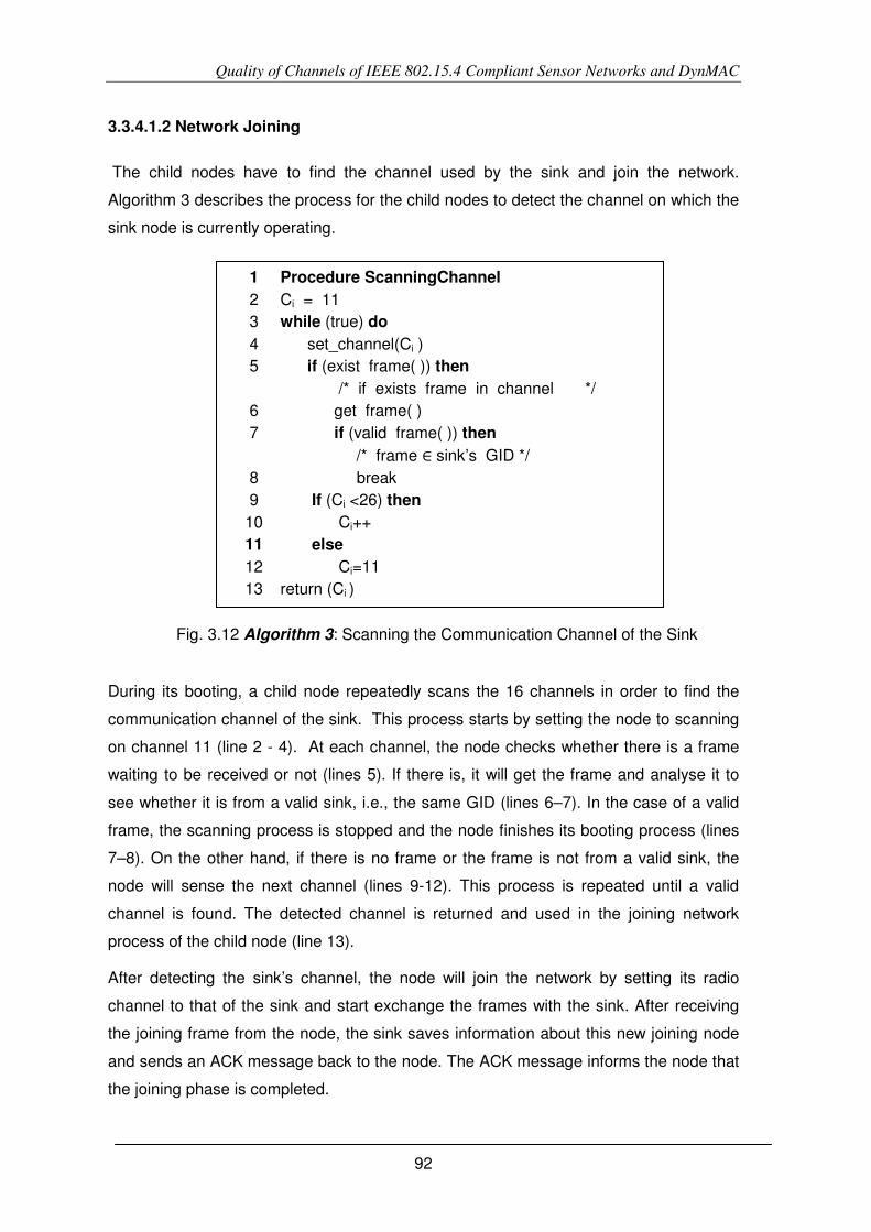
Quality of Channels of IEEE 802.15.4 Compliant Sensor Networks and DynMAC
92
3.3.4.1.2 Network Joining
The child nodes have to find the channel used by the sink and join the network.
Algorithm 3 describes the process for the child nodes to detect the channel on which the
sink node is currently operating.
During its booting, a child node repeatedly scans the 16 channels in order to find the
communication channel of the sink. This process starts by setting the node to scanning
on channel 11 (line 2 - 4). At each channel, the node checks whether there is a frame
waiting to be received or not (lines 5). If there is, it will get the frame and analyse it to
see whether it is from a valid sink, i.e., the same GID (lines 6–7). In the case of a valid
frame, the scanning process is stopped and the node finishes its booting process (lines
7–8). On the other hand, if there is no frame or the frame is not from a valid sink, the
node will sense the next channel (lines 9-12). This process is repeated until a valid
channel is found. The detected channel is returned and used in the joining network
process of the child node (line 13).
After detecting the sink’s channel, the node will join the network by setting its radio
channel to that of the sink and start exchange the frames with the sink. After receiving
the joining frame from the node, the sink saves information about this new joining node
and sends an ACK message back to the node. The ACK message informs the node that
the joining phase is completed.
1 Procedure ScanningChannel
2 Ci = 11 3 while (true) do 4 set_channel(Ci ) 5 if (exist frame( )) then
/* if exists frame in channel */ 6 get frame( ) 7 if (valid frame( )) then
/* frame ∈ sink’s GID */ 8 break 9 If (Ci <26) then
10 Ci++ 11 else
12 Ci=11 13 return (Ci )
Fig. 3.12 Algorithm 3: Scanning the Communication Channel of the Sink

Quality of Channels of IEEE 802.15.4 Compliant Sensor Networks and DynMAC
93
3.3.4.2 Global Best Channel Selection
Because the best channel chosen by the sink node only uses the local information at the
sin, it may not be a good channel for the entire network. The reason is that the noise
and interference at the child nodes might be different from those at the sink. Therefore, it
is necessary that all nodes in the network contribute to the process of choosing the best
channel. This process should be started when all the nodes have already joined the
network. However, in the real environment the full network may never be reached for
some reason, e.g. some nodes are not available. Therefore, we define a stable state for
the network. We consider a network is in stable state if there at least one child node
joined the network for long enough duration (e.g., 5 minutes). When the network is in
stable state, the process of choosing the best global channel is started. This process is
shown in Fig. 3.13 and consists of the following steps:
1. The sink node broadcasts messages to solicit information about the channel
conditions at other nodes. The broadcast message is sent 3 times to make sure
that all nodes receive at least one request.
2. When receiving the broadcast message from the sink, the normal node forwards
this message to its children. The node then samples the RSSI values on all
channels a number of times. The process of sampling of RSSI values is the
same as the one done at the sink in the local best channel selection process
(Algorithm 1).
3. The node then employs the Algorithm 2 to compute the cost of each channel and
to sort them in ascending order of the cost.
4. The ordered channel list (not RSSI values) computed by the normal node in step
3 is then sent to the sink.
5. When the sink has enough information from network nodes, it will decide which
channel is the best one. The process of choosing the global best channel is
described in Algorithm 4.
6. After choosing the best channel and it is different from the current working
channel, the sink will broadcast three switching channel messages to ask other
node to switch to the new channel.
7. When receiving the switching channel message from the sink, child node will
forward it to its children. To ensure that at least one of these broadcast
messages reaches the leaf node, the intermediate child nodes will wait at least
three switching channel messages or until a predetermined duration elapsed,

Quality of Channels of IEEE 802.15.4 Compliant Sensor Networks and DynMAC
94
e.g., 15 seconds. After the waiting condition passes, it will switch to new
channel.
8. The sink will switch to new channel after finishing sending the last switching
channel message.
Because the sink only gets an ordered list of channels (from the best one to the worst)
from the normal nodes in the network in order to decide which channel is the best one,
the procedure shown in Algorithm 4 is employed.
Computing and Selecting the global
best channel
5
Sink Child Node
Broadcast solicit
messages
1
Broadcast switching channel messages
6
Sensing 16 channels N times to collect needed
information
2
Computing the cost for
each channel and sorting them using index sorting
3
Sending the sorted
channel list to the sink
4
Switching to new channel
7
Switching to new
channel
8
Fig. 3.13 The Process of Selecting Global Best Channel.

Quality of Channels of IEEE 802.15.4 Compliant Sensor Networks and DynMAC
95
The global best channel is selected based on the total costs of channels. In order to
compute the total cost for channels, it is necessary to assign a cost for each position of
the ordered lists obtaining from the normal nodes. For simplicity, the cost of the channel
is also its position in the sorted list, i.e., the cost of the first position is 1, the second
position is 2, etc. Consequently, the total cost of each channel is calculated as described
in (lines 2–5). To avoid choosing the worst channel of some nodes in the network, i.e.,
the channel located in the last position of the ordered channels, the sink node also
stores a list of the worst channels (lines 6–7). The list of costs of the channels is then
sorted, in ascending order by cost, and stored in the channel_index_ global array (line
8). The global best channel is the channel in the lower position in the channel cost list
that does not appear in the worst channel list (lines 9–14). In case there is no such
channel, the channel in the first position of the channel cost list is chosen as best
channel.
1 Procedure GlobalBestChannel /* Compute the cost for each channel */
2 for (node_id ∈ nodeList) do 3 for (pos in 0..15) do
/* get the channel at pos */
4 channel = Channel_index_list[node id][pos] 5 channel cost[channel]+=pos+1
/* Store the worst channel list */ 6 if (channel index list[node_id][pos] == 15) then 7 bad_channel[channel]+=1
/* Sorts channels by cost and store in channel index global */ 8 Sort_channel(channel_cost, channel_index _global)
/* Choosing the best channel */ 9 best _channel = channel _index _global[0]
/* Reselect the best channel if it exists in bad_channel_list */
10 c=0; 11 while ( (c < 16)&&(bad _channel[c] > 0) ) do 12 c++ 13 If (c<16) 14 best_channel = channel_index_global[c] 15 return best_channel
Fig. 3.14 Algorithm 4: Choosing the Global Best Channel.

Quality of Channels of IEEE 802.15.4 Compliant Sensor Networks and DynMAC
96
3.3.4.3 Periodically Re-evaluating the Best Channel
Because the quality of the channel may vary with time, the best channel at one period
may become the worse (e.g., high lost rate) during the operation of the network. As a
result it is necessary to periodically re-evaluate the quality of the channels. Two possible
approaches are: (1) the sink periodically sends the request to the normal nodes to solicit
the channel information to re-evaluate the best channel (2) the nodes periodically
evaluate the quality of the current channel based on different metrics, such as error rate
or on the number of lost links, and send this information to the sink.
In DynMAC, the second approach is employed using the PER as the evaluation metric.
Every normal node periodically checks its PER and if it is higher than a threshold (e.g.,
1%), the node will send a message to the sink stating this information. When the sink
receives the information, it will decide whether there is a need to re-select the global
best channel. In our implementation, the sink makes the decision based on the number
of nodes that send the re-evaluation request. Because the sensor networks usually
operate for a long time if the pure accumulated PER is used for evaluating the current
condition of the channel then it will take very long for detecting dynamic noise and
interference. Consequently, DynMAC employs the PER over a predefined time interval,
to evaluate the channel condition. Particularly, in our implementation, we use the PER of
the last 5 minutes as the evaluation metric. The best channel re-evaluation process is
the same as the process of the global best channel selection described in previous
section.
3.3.4.4 Recovery from Connection Loss
During network operation any node may lose the connection to its parent for different
reasons. One example of such scenario is that the node did not receive a switching
channel message from the sink. In this case, the sink switches to the new channel,
leaving the node working in the old channel. Therefore, it is necessary to have a
mechanism for the node to recover from such a situation. To resolve this issue, the
node is forced to re-scan the communication channel of the sink if it cannot
communicate with its parent for a specific duration. To do this, a child node runs the
Algorithm 3 to scan the sink’s channel.

Quality of Channels of IEEE 802.15.4 Compliant Sensor Networks and DynMAC
97
3.3.5 Experiments and Results
In order to evaluate the mechanisms implemented in the DynMAC protocol, the Contiki
operating system [95], together with TelosB [47] sensor nodes, was used. As a first
step, DynMAC was evaluated using the COOJA simulator [171], [172] provided together
with ContikiOS. COOJA simulator was used to make a first evaluation of the settings
that would be used later in the real testbed. The structure of the network used for
experiments is shown in Fig. 3.15. Within this network, the number of slots of the super-
frame was set to 100. Therefore, each super-frame has 1000 ms (10 ms per slot).
3.3.5.1 Experiments with Simulation
COOJA simulator [171], [172] was used to test the functionality of the proposed
algorithms. Specifically, the scanning, the coverage, and the handoff time were
measured.
Fig. 3.15 Testbed sensor network
n-0-0-0
n-1-1-0
n-2-0-0 n-1-0-0
n-1-1-1 n-1-1-2
n-2-1-0
n-2-1-1 n-2-1-2
n-3-0-0
n-3-1-0
n-3-1-1 n-3-1-2

Quality of Channels of IEEE 802.15.4 Compliant Sensor Networks and DynMAC
98
3.3.5.1.1 Scanning and Network Coverage Time
The first simulation was done to evaluate the scanning and the network coverage time.
For the scanning time, it measured how long it takes for the nodes at different levels to
detect the channel on which the sink is currently working. For the network coverage
time, it is measured the time for all nodes to successfully join the network. In these tests,
we measured the time from the moment when the sink finished its booting. The results
of the experiments concerning the scanning time are shown in Table 3.2 and in Fig.
3.16.
As shown in Table 3.2, some nodes at level 1 can immediately detect the channel on
which the sink is running during, i.e., on the first super-frame (112ms). The scanning at
this level has a maximum of 9 super-frames (8648 ms), and an average of about 4
super-frames (3842.68 ms). For the nodes at Levels 2 and 3, they also take the similar
amount of time to detect the channel of the sink (or its parent). It means that the node
can detect its parent on the first super-frame. Furthermore, most of the nodes (75
percent) can detect their parents during the first 5 super-frames (4860ms). However, for
the node at Level 3, sometimes it takes a little bit longer up to 15 super-frames (14264
ms).
In addition to the scanning time, the nodes also need time to initialize the parameters for
their environment to finish the booting process. In most cases, it takes a node less than
600ms to finish its booting. In our experiments with the simulation, after the detection of
the parent channel, the node needs a maximum of 729 ms. From Table 3.2 we can
estimate the coverage time of the network, that is, the maximum duration for all nodes in
the network to detect and join the network. In this case, the coverage time was less than
Table 3.2 Scanning and Booting Time of Nodes at Different Levels (Simulation)
Statistic Level 1 Scanning time (ms)
Level 1 Finish
booting time (ms)
Level 2 Scanning time (ms)
Level 2 Finish
booting time (ms)
Level 3 Scanning time (ms)
Level 3 Finish
booting time (ms)
Minimum 112 160 24 72 24 136
Q1 2228 2652 784 1170 822 1074
Median 3798 4054.5 2104 2352 2236 2468 Q3 4860 5462 2483.75 2753.25 4264 4554
Maximum 8648 8920 8872 8984 14264 14856 Average 3842.68 4175.21 2309.26 2569.97 3056.15 3332

Quality of Channels of IEEE 802.15.4 Compliant Sensor Networks and DynMAC
99
33 seconds (8920ms + 8984ms + 14856ms = 32760ms). We also repeated this
experiment numerous times to measure this coverage time and in all the experiments it
took less than 17 seconds (maximum 16920ms).
3.3.5.1.2 Handoff Time
In this context, handoff time is the time that a node (e.g., mobile nodes) takes to rejoin
the network, that is, resynchronize itself with its parent after leaving the network. From
the simulation, it takes from 3 ms to 384ms for a node to resynchronize with its parent
node. If this node is not a leaf, its children also have to resynchronize with it and with the
sink. From the experiments, it is very fast for other nodes to resynchronize with its
parent (maximum 678ms).
3.3.5.2 Experiments With Testbed
In addition to simulation, we also set up a testbed using TelosB motes [47], and using
the same topology as depicted in Fig. 3.15. The objective of the experiments using
testbed was to validate the mechanisms proposed in DynMAC. More important, the
experiment with the testbed proved that the proposed solution is feasible.
Fig. 3.16 Scanning and Booting Time at Different Levels (Simulation).
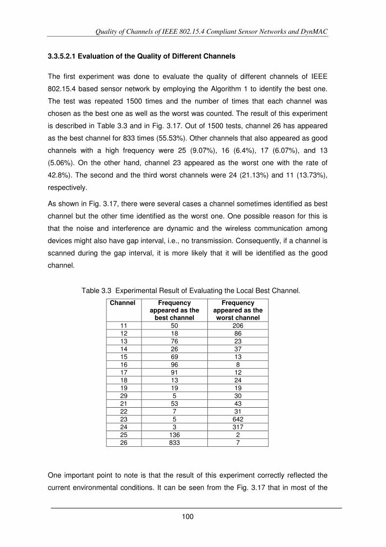
Quality of Channels of IEEE 802.15.4 Compliant Sensor Networks and DynMAC
100
3.3.5.2.1 Evaluation of the Quality of Different Channels
The first experiment was done to evaluate the quality of different channels of IEEE
802.15.4 based sensor network by employing the Algorithm 1 to identify the best one.
The test was repeated 1500 times and the number of times that each channel was
chosen as the best one as well as the worst was counted. The result of this experiment
is described in Table 3.3 and in Fig. 3.17. Out of 1500 tests, channel 26 has appeared
as the best channel for 833 times (55.53%). Other channels that also appeared as good
channels with a high frequency were 25 (9.07%), 16 (6.4%), 17 (6.07%), and 13
(5.06%). On the other hand, channel 23 appeared as the worst one with the rate of
42.8%). The second and the third worst channels were 24 (21.13%) and 11 (13.73%),
respectively.
As shown in Fig. 3.17, there were several cases a channel sometimes identified as best
channel but the other time identified as the worst one. One possible reason for this is
that the noise and interference are dynamic and the wireless communication among
devices might also have gap interval, i.e., no transmission. Consequently, if a channel is
scanned during the gap interval, it is more likely that it will be identified as the good
channel.
One important point to note is that the result of this experiment correctly reflected the
current environmental conditions. It can be seen from the Fig. 3.17 that in most of the
Table 3.3 Experimental Result of Evaluating the Local Best Channel.
Channel Frequency appeared as the
best channel
Frequency appeared as the worst channel
11 50 206 12 18 86 13 76 23 14 26 37 15 69 13 16 96 8 17 91 12 18 13 24 19 19 19 29 5 30 21 53 43 22 7 31 23 5 642 24 3 317 25 136 2 26 833 7

Quality of Channels of IEEE 802.15.4 Compliant Sensor Networks and DynMAC
101
time the channel the channel 23 and 24 were identified the worst ones. The reason is
that there is an IEEE 802.11g wireless Access Point (AP) operating on the channel 11
positioned very near the sink (1 meter). Consequently, this AP significantly affects the
quality of the channels of IEEE 802.15.4 based WSNs. Similarly, the experimental result
also showed that 26 and 25 were selected as the best channel with a very high
frequency. It is explicable because, in the experimental location, these channels did not
interfere with other wireless networks. For other channels, because there are many WIFI
networks operating on the channels 1, 6, and 11, their quality depends on the traffic rate
of these networks. In fact, as shown in Fig. 3.17, there are still some good channels that
can be used for WSNs such as channel 16 and 17.
To evaluate the differences in performance between the identified good channels and
worse ones, we did numerous experiments with three best channels (26, 25, and 16)
and three worst ones (23, 24, and 11). In these experiments, the packet loss rate of
each selected channel was measured with two MAC protocols: X-MAC [62] and
DynMAC. The objective of this test was not to compare the performance between these
two protocols but to see how they perform on the different channels. Because X-MAC
[62] is a CSMA based MAC protocol, we set up a testbed with only two nodes: one for
sending packets and the other for collecting packets and calculating the packet loss
rate. The reason for this simple testbed was to avoid the internal interference among the
Fig. 3.17 The Quality of Channel at the Sink

Quality of Channels of IEEE 802.15.4 Compliant Sensor Networks and DynMAC
102
nodes in the WSN. The testbed for the DynMAC has the same topology described in
Fig. 3.15. The result of these experiments is shown in Fig. 3.18.
It can be seen from Fig. 3.18 that there is a significant difference in loss rate between
the best and worst channels. With X-MAC, a simple two-node testbed, the packet loss
rate of the worst channel was more than 6% while that rate of the best channel was less
than 3%. For the DynMAC, because it is a TDMA protocol with the acknowledgment
and retransmission mechanism, the loss rate was significantly reduced. However, there
is still a noticeable difference between the best and the worst ones. For the worst
channel, the loss rate could be up to more than 3% while that rate for the best one is
about 0.25%. Considering the experimental results, it could be concluded that the
selecting the right communication channel could significantly improve the performance
of a WSN.
3.3.5.2.2 Scanning and Network Coverage Time
The next experiment we did was to measure the scanning time of the nodes and the
network coverage time. The former refers to the time it took for a node at different levels
to detect the channel on which the sink is currently running was measured. On the other
hand, the latter measures the total time it takes for all nodes to successfully join the
network. In these tests, the time was measured from the moment when the sink node
finished booting. The experimental results concerning the scanning time using
simulation are shown in Table 3.4 and Fig. 3.19.
Fig. 3.18 Loss Rate of Good vs Worse Channels.

Quality of Channels of IEEE 802.15.4 Compliant Sensor Networks and DynMAC
103
As shown in Table 3.4, it is very fast for a node to scan and detect the channel of its
parent. In most cases the nodes only take 1 super-frame (less than 1 second) to detect
the communication channel of the sink. However, in some cases, it takes up to 3 super-
frames (2120 ms) to scan the operation channel of the sink node, a situation that occurs
mainly from nodes at a level far away from the sink. This is reasonable because nodes
at higher levels have to wait for their parents to join the network before they can detect
them.
Fig. 3.19 The Scanning and Booting at Different Levels (Testbed)
Table 3.4 Scanning and Booting Time of Nodes at Different Levels (Testbed)
Statistic Level 1 Scanning time (ms)
Level 1 Finish
booting time (ms)
Level 2 Scanning time (ms)
Level 2 Finish
booting time (ms)
Level 3 Scanning time (ms)
Level 3 Finish
booting time (ms)
Minimum 16 168 8 88 8 88
Q1 120 432 160 392 160 376
Median 424 832 384 720 336 668
Q3 688 1048 664 1048 658 954
Maximum 984 1352 1328 1720 2120 3496
Average 432.35 745.41 459.63 794.35 477.24 761.41

Quality of Channels of IEEE 802.15.4 Compliant Sensor Networks and DynMAC
104
Similarly to the simulation result, after knowing the channel of the sink node, the nodes
need time to finish its booting. Observing the experimental results obtained from the
testbed, we saw that this duration was similar to those obtained from simulation.
However, in some cases, it takes a little bit longer for the node to finish booting. In our
experiments, there was a case where it took 1696 ms for a node to finish booting after it
detected the channel. As shown in Table 3.4, the coverage time of the network can be
estimated and it takes less than 7 seconds: (1352ms maximum booting time at level 1 +
1720ms maximum booting time at level 2 + 3496ms maximum booting time at level 3 =
6568ms). We did numerous experiments to measure the network coverage time. And
most of the time it took about 3 seconds for all nodes to form the entire network. In
addition, the maximum network coverage time was about 6040ms.
3.3.5.2.3 Dynamic Noise and Interference Detection
Besides the ability to select the best channel automatically, DynMAC is also able to deal
with dynamic noise and interference, which occur during the sensor network’s operation.
The mechanism how DynMAC can realize this function is described in Section 3.3.4.3.
To prove that the proposed mechanism is applicable and workable solution, we did
numerous experiments. In the experiments, the time interval for computing the PER was
set to 5 minutes and the threshold was 1%. It means that if the PER of the last 5
minutes is equal or greater than 1% then the normal node will send an alert message to
the sink. In addition, if the sink receives 3 or more alert messages from the nodes it will
start the best channel re-evaluation process.
In order to evaluate this functionality of DynMAC, during the normal operation of the
WSN, we tried to introduce the interference in its currently communication channel (e.g.,
channel 26). We did this by putting 4 sensor nodes continuously broadcast on the
working channel of the sensor network. The interference caused by these 4 sensors
affected the PER of some nodes in the network. Consequently, these affected nodes
detected the interference and sent warning messages to the sink. Observing the
operation of sensor network, we recognized that after introducing interference about 10-
15 minutes the sink started the best channel re-evaluation process. In addition, the
effect of this process was that the sensor network was switched to a new channel, e.g.,
from channels 26 to 25.

Quality of Channels of IEEE 802.15.4 Compliant Sensor Networks and DynMAC
105
3.3.5.2.4 Recovery from Connection Loss
Another type of experiment we did was to evaluate the ability of a node to recover from
the connection loss. It is important to note that the connection loss in this context is
mainly referred to the case in which the normal nodes did not receive any switching
channel request message from the sink. The result of such a scenario is that the sensor
network switches to operate on another communication channel but some specific
nodes. Consequently, these nodes have to somehow resynchronize themselves with the
sink to continue to communicate.
In order to test whether this functionality can be achieved, during the switching channel
process we moved a node to a place in which it could not communicate with its parent.
Then, after the sensor network successfully switched to the new channel, that node was
moved back to its original position. We did a number of experiments with two types of
normal nodes: leaf and intermediate nodes. The experimental result showed that it is
very fast for these nodes to detect its parent and re-establish its communication. In
most cases, it took a node about 3 seconds, with maximum less than 10 seconds, to
resynchronize with its parent.
3.4 Summary
The work presented in this chapter focuses on the reliable communication of the WSNs.
It first discusses the experimental studies of the characteristics of channels of 802.15.4
compliant sensor networks. The results of this study show that the quality of channels of
WSNs depends on the deployment environments and varies with time. In addition, it is
difficult to predict the quality of different channels based on theoretical models.
Consequently, empirical study is the appropriate method for choosing the appropriate
channel when deploying sensor networks. More importantly, this chapter presents our
proposed MAC protocol, DynMAC, to allow WSNs to coexist with other wireless
networks as well as to operate in noisy environments. The proposed protocol adds
additional reliable level to GinMAC by allowing the WSN to dynamically adapt to the
noise and interference conditions of the deployment environment. In particularly, it
employs the mechanisms for best channel evaluation, noise and interference detection,
and lost communication recovery. DynMAC were successfully evaluated using both
simulation and real testbed. The experimental results showed that our mechanisms
resolve the configuration problems of the WSN in noisy and interference environments
while maintaining the application requirements under critical scenarios.

Sensor Traffic Description Language (STDL)
106
4 The Integration Framework and Sensor Traffic Description
Language (STDL)
Summary
4.1 Introduction
4.2 The Interoperability Model
4.3 Sensor Traffic Description Language (STDL)
4.4 STDL engine
4.5 Prototype and Sample Applications
4.6 Summary
SNs are considered the bridge between physical and digital worlds, and
they are envisioned to become an integral part of our daily life as well as
an important element of the Future Internet. Therefore, integrating WSNs
into external networks and applications is an undeniable requirement. The problem of
current integration solutions for WSNs is their adaptability, i.e., the ability to reuse
gateways and proxies in a multitude of sensor networks with different types of protocols
and data frames. One reason behind this problem is that it is difficult or even impossible
to standardize the structure of data inside the frame because there are a huge number
of possible formats. Consequently, it is necessary to have a mechanism to deal with this
problem. Our approach for this problem is to propose a framework that uses a language
for describing the traffic in sensor networks named Sensor Traffic Description Language
(STDL). In order to reuse the framework on a new sensor network, it is only necessary
to describe the network’s frame structures using STDL. This chapter details proposed
framework, STDL and its prototype implementation.
W

Sensor Traffic Description Language (STDL)
107
4.1 Introduction
The major applications of WSNs are monitoring and controlling their target
environments. They are as a bridge between physical to digital worlds. Therefore, in
most cases, WSNs cannot operate in a complete isolation, but they need to be
monitored and/or managed by control centers, which hosts Supervisory Control and
Data Acquisition (SCADA) systems or other applications. The interoperability between
WSNs and the external applications is a challenge because of their differences in
communication protocols as well as diversity of possible sensor data formats. The
solution for this problem is either to implement the same protocol on both environments
or to add a gateway and/or a proxy between them.
Interconnecting WSNs with IP networks is desirable because it offers the opportunity to
integrate WSNs with the future Internet, i.e., Internet of Thing (IoT). The recent
researches have been proven that it is possible to implement both IP protocol stack
[173], 6LowPAN [15] and web services [17], [18], [19], [20] on the sensor nodes.
However, the limitations of sensor nodes in terms of memory, computation,
communication and power source make it difficult and inefficient to deploy the full
TCP/IP protocol stack and web services into all sensor nodes. Consequently, some
optimal mechanisms such as header compression [15], Message Compression [20],
packed JSON [18], EBHTTP [103], UDP binding [18], [20], etc need to be applied to the
original standards to make it feasible for sensor nodes. As a result, the current solutions
for interconnection such as 6LowPAN [15] and integration such as Tiny web services
[17], WoT [19], and sMAP [18], and CoAP [20] still needs a bridge, proxy or gateway for
the external applications to interact with sensor networks. In addition, allowing directly
access to sensors from the Internet brings many challenges such as security, energy
efficiency, and routing. Consequently, integrating IP stack and web services to sensor
nodes is not a solution for all types of WSNs. As a matter of fact, the gateway or proxy
approach for interoperating between WSNs and external applications will continue exist
in the foreseeable future.
Other works on integrating WSNs with the external environments includes GSN [13],
SensorWeb [104], VIP Bridge [12]. The common feature of most of these works,
excluding VIP Bridge, is that the data, and/or functionalities of sensor nodes and
networks are exposed as web services, which make the interoperability with applications
over Internet easier. However, the problem with the current gateway-based integration
solution is their adaptability. i.e., the gateway or proxy is not adaptable to different types
Sensor Traffic Description Language (STDL)
108
of data formats. This means that the new drivers or parsers need to be developed when
applying the gateway or proxy for a new sensor network or when adding new sensors
or applications to existing one.
The Open Geospatial Consortium's (OGC) [173] has been working on series of
specification named Sensor Web Enablement (SWE) for making sensors and sensor
systems discoverable, interoperable over the Internet. SWE consists of a series of open
standard specifications for discovery of sensors and sensor systems, for exchanging
and processing sensor observation, and for tasking of sensor and sensor system. The
SWE standards can be divided into 2 groups: (1) Models and schemes for encoding
sensors and sensor observations; and (2) open web service interfaces. The former
consists of Sensor Model Language (SensorML) [175], Observations and
Measurements (O&M) [176]. The latter comprises Sensor Observation Service (SOS)
[177], Sensor Planning Service (SPS) [178], and PUCK [179]. The SOS offers the web
service interface for the client applications to retrieve the measurement and the
description of sensors and sensor systems. The response formats of the SOS are XML-
based data encoding using SensorML or O&M. SensorML is used to encode the
descriptions while O&M is used for the measurements and observations from the
sensors and systems. In addition, the user can task the sensors to perform appropriate
actions through SPS web service interface. The SPS provides a list of observations that
the users can assign to sensors or sensor networks. These four standards allow the
clients applications to discover, and to access the sensors’ measurement as well as to
task the sensors via gateway. The PUCK protocol [179] was integrated into SWE in
2011 to enable plug and play sensor networks.
The above solutions provide a method for client applications to access the sensor data
through the gateway. An equally important aspect is how the gateway interacts with the
sensors and sensor networks. This means how the gateway can discover and analyze
the data from sensors and sensor networks to make it available for use by the
application and how it can send the commands to the WSN. The traditional approach for
this problem is to request the sensor nodes to format the data according to the format
required by the provided drivers [13]. Another method is to add a software driver or
analyzer for each sensor or data frame format [13], [104]. In order to make the sensors
as plug and play components of the gateway, the IEEE 1451 family standards [180] has
been proposed. One of the core components of this family standard is the definitions of
Transducer Electronic Data Sheets (TEDS), which are embedded into the transducers
(sensors or actuators), to allow the interoperability between different manufacturers, and

Sensor Traffic Description Language (STDL)
109
to make their data analyzable. Although it provides a standard way to exchange data,
the software drivers and TEDS documents also needed to be manually developed and
installed on every sensors. Recently, SWE integrated PUCK protocol [179] to store and
automatically retrieve metadata and other information to/from the sensor nodes. The
information stored in the nodes’ memory is called PUCK memory and may include the
IEEE 1451 TEDS, SensorML, or even the driver code. The gateway, which supports
PUCK protocol, can automatically retrieve and utilize the information from sensor when
it is installed [179]. In addition, if the driver code is available on the sensor node, it is
downloaded into and executed on the host to translate the sensor raw data, using TEDS
or SensorML, into the required format, e.g. OGC O&M object. The PUCK protocol brings
another level of plug and play capability for sensor devices. However, it requires
implementing PUCK documents on every sensor devices. In addition, to make a device
as plug and play component the driver code has to be physically stored in the PUCK
memory before deployment. Consequently, it is not appropriate for WSNs that
comprises many sensor nodes.
Making the interoperability framework adaptable to different types of WSNs is
challenges for several reasons. First, each type of sensor networks may have its own
data frame structures and the organization of data inside a frame also contributes to this
complexity. The problem is that the data from sensor networks is mainly consumed by
the front-end applications, not directly by the end users. Therefore, only a minor change
in the data section of a frame produces a totally different frame, and it leads to
innumerous possible data formats. For instance, assuming that a sensor node has a
frame containing two data fields (e.g., temperature and humidity), and if for some
reason, the positions of these two fields is swapped. For the machine, this is a totally
different frame, and it requires modifying the program code to analyze the content of the
frame. Consequently, the gateway or proxy has to be modified (reprogram or add new
methods) every time there is a change in the data frame formats.
Bearing in mind the previous points, the work in this chapter focuses on a solution for
analyzing and extracting useful data from every sensor data frame between the
framework and WSNs. Our approach to this problem is to propose the Sensor Traffic
Description Language (STDL), which describes the possible data frame formats
presented in the sensor networks. It plays a similar role to PUCK documents. However,
it does not require adding the description documents to every sensor but only to the
proxy. For the interaction with client applications, the proposed framework employs open
web services standards similar to those of SWE [174]. However, in order to make it easy

Sensor Traffic Description Language (STDL)
110
and more compact to integrating with application platforms such as Facebook [181],
Second Life [182], the RESTful web services [101] and encoding method similar to
those used in sMAP [18] are employed. The following sections present the proposed
model, STDL, its prototype and illustration applications.
4.2 The Interoperability Model
The main aspects that were concerned when designing this model were the
interoperability, reusability, scalability and extensibility. The first aspect refers to the
ability of the gateway to provide methods for other application environments to easily
and transparently interact with sensor networks. In addition, the interface for accessing
the internal sensor data and functionalities should be unified and standardized. The
reusability, in this context also called adaptability, is the ability to use the proposed
model for different WSNs without reprogramming or modifying. The third concern is
about the ability of the model to handle the increase in the number of sensor nodes and
sensor networks. The final aspect, extensibility, is about the ability to easily add new
components to the model. Consequently, we come up with a general model as it is
presented in Fig. 4.1. The details on how to obtain the above-mentioned objectives will
be discussed in the following paragraphs and sections.
In order to create a system that is able to respond to a large number of concurrently
requests, we employed a multi-layered software architecture. As shown in Fig. 4.1 the
model uses the proxy and gateway as a mediate layer for interoperability between
sensor networks and the external applications, which monitor and control them. The
proxy interacts directly with the WSNs, getting and analyzing data frames from the
sensor networks, and then sending them to the gateway for storage. It also passes
commands from the user applications to the sensor networks. The gateway allows
front-end applications to interact with sensor networks, acting as a bridge between the
sensor networks and the Internet. Both proxy and gateway may also comprise some
other facility services such as authentication and authorization.
Both proxy and gateway are designed using the event-based principle. To add a new
component to the framework, developers can register the listeners that capture events
of interest that happen in the sensor network. For instance, to support the localization,
the positioning client registers to the “data frame arrival” event of the proxy to get the
necessary information to send to the localization engine on the gateway. This event-
based model allows the system to be extensible easily.

Sensor Traffic Description Language (STDL)
111
It is worth noting that every sensor network is associated with at least one proxy, and a
proxy could serve more than one sensor networks. Every proxy is associated with at
least one gateway to communicate the traffic of the sensor network to the data storage.
There can exist multiple proxies and gateways in a single network. This type of
architecture makes the proposed model scalable to apply for large sensor networks.
4.2.1 The Gateway
The gateway, also called web service gateway, is the entry point that allows front-end
applications to interact with the sensor networks. The gateway hosts the middleware
that implements the main functionalities of the system. The core components of the
middleware are depicted in Fig. 4.2. The gateway uses a database for storing the
sensed data and other necessary data.
SCADA Enterprise Application
Virtual World/ Web 2.0
Mobile Application …
Interoperability Infrastructure
Sensor Networks
Gateway
Proxy Proxy
Proxy
Front End
Fig. 4.1 The General Model for Interoperability

Sensor Traffic Description Language (STDL)
112
The middleware provides a set of input adapters and a command sender to
intercommunicate with sensor networks or other smart devices through the proxies. The
Input Adapter accepts the sensor data from the proxy and stores it into the data storage
by using the repository service. It also accepts the localization requests from the proxy.
On the other hand, the Command Sender is used to send commands from the control
application to the sensor networks. Both Input Adapters and Command Sender can be
implemented using several protocols including sockets, JMS, XML-RPC and web
services. The current implementation is web service, i.e., the communication between
proxies and the gateway uses web services.
In order to make the seamless interoperability between the sensor networks and the
font-end applications, the data and functionality of sensor networks are exposed using
web service (Web Service Interfaces component). The data from the sensor networks
can be retrieved through the web service interface, stored and visualized from
everywhere. The main advantage of the web service is that it isolates the services from
the consumers. In addition, any changes of the middleware will not affect the
applications consuming the services provided that its interfaces keep intact.
The web service interface component is supported by three essential components: (1)
Query service; (2) Command service; and (3) Event manager. The first component is
responsible for processing the query requests from the external applications. If the
request is for data, it will search the appropriate data from the storage and send it to the
corresponding application. On the other hand, if it is a command, then the Command
Service will take its role to process and send the request to the sensor network via proxy
using the Command Sender. In the case of periodical requests (tasking), the Event
Manager will process this type of demands. It employs the publisher-subscriber pattern
to allow client applications to register for the events of interest.
Commands to WSN
Web
serv
ice In
terf
aces
Inp
ut
Ad
ap
ters
Co
mm
an
d
Sen
der
Storage
Data from proxies
Repository Service
Query Service
Localization Service
AAA Service Requests from
user applications
Event Manager
Command Service
Fig. 4.2 The Core Components of Middleware of the Gateway

Sensor Traffic Description Language (STDL)
113
Equally important, the middleware of the gateway also integrates some other useful
services such as Authentication, Authorization and Auditing (AAA), and localization
service. The AAA service provides the basic security for the system. The localization
service is responsible for estimating the location of the device. This service is very
useful for numerous applications, namely health-care and monitoring workers in
hazardous environments. The details of localization service will be presented in chapter
5.
4.2.2 The proxy
It is worth noting that the gateway is not a standalone entity, but it needs the presence of
its collaborators, i.e., the proxies, to feed it with data as well as to allow it to send the
commands to sensor networks. The proxy is responsible for obtaining the data frame
from the sensor network, analyzing and publishing them to the gateway. In addition, it
also accepts commands from the user applications, and sends them to the sensor
networks. The core components of the proxy are shown in Fig. 4.3.
The interaction between proxy and gateway is via their corresponding components. In
particular, the Data publisher component of the proxy is responsible for forwarding
sensor data to the Input Adapters component of the gateway for storage. The proxy also
supports localization by using the Location Requester to send the requests to the
location engine on the gateway. Similarly, the Request Receiver component of the proxy
To the Gateway
From WSNs
To WSNs
STDL
Raise Event
STDL Engine
0111…1010
Tra
ffic
L
iste
ners
C
om
man
d
Sen
der
Data
P
ub
lish
er
Req
uest
Receiv
er
Temp:20
1101…0010Command
From the Gateway
Lo
cati
on
R
eq
ueste
r
Fig. 4.3 The Components of the Proxy

Sensor Traffic Description Language (STDL)
114
accepts the commands from the user application via the Command sender component
of the gateway.
Another important component of the proxy is the Traffic Listener that listens for the data
from sensor networks. Because there are several methods for sensor networks to
communicate with the proxy (e.g., the serial port or TCP/IP), it is necessary to have
different types of listeners, one for each communication method. The traffic listener
simply listens for incoming frames, and then forwards them to the STDL engine for
further processing. Currently, we implemented two types of traffic listeners on the proxy:
one for serial port and the other for IP communication.
It is important to note that the most important component of the proxy is the STDL
engine which makes the proxy be adaptable with different sensor networks. It is
responsible for translating the raw data frame into the meaningful data for other
components. When receiving a raw frame from the listener, the STDL engine translates
it into the one or more messages and raises the corresponding data events, which are
handled by other components such as the Data Publisher or Localization Requester.
The Data Publisher, when triggered by a data event, gets associated message and
sends it to the gateway for storage. The Location Requester collects the necessary data
from multiple events and sends them to gateway’s localization engine, which estimates
the position of a device. The structure of the event message will be detailed in the
following section.
In addition to translating raw frame to data message, the engine also translates the
commands from the user applications into the format that the sensor nodes can process.
When receiving user application commands from the gateway through Request
Receiver, the STDL engine translates them into a format that the sensor nodes can
process. The engine then passes the commands to the Command Sender component
which sends it to the sensors.
The most important point to note is that the STDL engine is independent of the type of
sensor networks. This means that it can be used for any sensor networks without
reprogramming. In addition, the crucial element that makes the engine and thus the
framework adaptable to different types of sensor networks is STDL. The details of the
STDL and how it can help to do this are presented in the following sections.
Sensor Traffic Description Language (STDL)
115
4.3 Sensor Traffic Description Language (STDL)
In order to make the proposed model adaptable to diversity of sensor networks’
protocols and applications, we proposed a language for describing the traffic of sensor
networks named Sensor Traffic Description Language (STDL). The objective of SDTL is
to formally and precisely describe the structures of data frames in WSNs so that the
proxy, i.e., STDL engine, can extract needed data fields from the frames. It plays the
similar role as those of IEEE 1451 TEDS [180] or PUCK documents [179] in that they
describe the sensors and the measurements. However, it differs from these two
standards in several ways. First, it only focuses on the data frame formats and the
needed information. This means that it does not include detailed information such as
manufacturer, serial number, etc. In addition, STDL documents only need to be put in
the proxies and not in every sensor nodes. Moreover, it does not require a description
for each sensor but one description for a group of sensors that produce the same data
frame format.
The motivation of this work is to reduce the complexity as well as the time for developing
the monitoring and controlling applications development for sensor networks. Normally,
the developers have to develop a special module or method (i.e., frame analyzer) to
extract the data for each type of raw frames in a specific sensor network. This work is
tedious, time consuming, and error-prone. In addition, even a small change in the
network such as adding a new type of sensor or modifying the structure of a frame also
requires reprogramming the analyzer. This means that the analyzer is very sensitive to
data formats of the frame. With our proposed approach, when there are any changes to
the current network or when applying it to a new sensor network, we only need to
describe the structure of the new frames using STDL and add this description into the
engine.
4.3.1 Overview of the Language
The aim of STDL is to add the adaptability to the infrastructure for interoperability
between sensor networks and application environments, and to simplify the application
development process. To provide this functionality, STDL has to be general enough to
describe the structures of as many types of sensor networks’ data frames as possible. In
addition, it must be formal and concise, and be able to be completed in computer
programs. Equally important, it should be simple and easy to use. Consequently, we

Sensor Traffic Description Language (STDL)
116
decide to employ XML as the based language, i.e., it uses the tags to describe data
frame structures.
Like other languages, STDL provides a set of key words (vocabulary) and rules
(grammar) to constrain how the key words are combined together to describe the
structure of data frames as well as permissible content of the data. As STDL is an XML-
based language, it is natural to use XML schema (XSD) [183] to create its constraint
rules. Because XSD is a text-based language, reading its content directly is very tedious
and difficult to follow. In addition, it will be difficult to convey the concepts to other
interested people. Therefore, it is useful to present the syntax of the language
graphically. Consequently, we employ the notations used in [184] and [185] to create the
content model diagram of STDL. The meaning of these notations is described in Table
4.1.
Table 4.1 The Notations Used in the Content Model Diagram
Notation Description
An optional element or attribute, i.e., min occurrence: 0 and max
occurrence: 1
A required single element or attribute, i.e., min occurrence: 1 and max
occurrence: 1
A repeated required element, i.e., min occurrence: 1 and max
occurrence: unbounded
Note:
- If the min occurrence is 0 then this element becomes a repeated optional
element and the line around it becomes a dash line instead of solid line
- The max occurrence could be any number greater than 0, e.g., 5
An element with simple content, i.e., it only contains text
An element with complex content, i.e., it can contain other elements or
attributes
An element with complex content that has child elements
A sequence of elements

Sensor Traffic Description Language (STDL)
117
A choice of elements
Represent a list of attributes or constraints of an element
Represent a complex type inside the content model diagram
Represent a complex type as a global element
With regard to designing a language to describe the traffic in sensor networks, there are
several essential aspects that need to be considered. The first and crucial one is how to
uniquely determine the type of each frame because a program can only extract the
useful data fields when frame is correctly identified. It is generally considered that the
frame type field can be used to identify the structure as well as the data inside the
frame. However, in some cases the frame type field does not uniquely identify the frame
but a group of frames instead. For instance, with the Internet Control Message Protocol
(ICMP), to uniquely identify a message an application has to combine two fields: the
type and the code (subtype). Accordingly, we have to take into account these points
when designing STDL.
The second key aspect is the structure of the data in a frame. Because the data from
sensor networks are consumed by the applications not directly by the end user, it is
important for the application to know exactly how to extract needed data from a specific
frame, i.e., the fields and their positions, correspondingly. From working experiments
with sensor networks, we divide the frames in WSNs into three main categories: simple
frames, data table frames and complex frames. The first category is the frames that
merely consist of a list of the data fields such as temperature and humidity. The second
type contains a list of data row in its payload, and each row contains a list of data fields.
The final type includes the frames that contain a list of other frames inside its payload,
i.e., a list of simple frames or a list of data table frames or a mixed list of both types.
All these issues will be carefully examined in the STDL and discussed in the following
subsections.
Type name

Sensor Traffic Description Language (STDL)
118
4.3.2 The General Content Model of STDL
As it is an XML-based language, it is natural to use XML Schema (XSD) [183] for
creating its constraint rules. To make the description of the language easily to
understand and apply, we present the language using the graphical notations described
in Table 4.1. The key components constitute a frame is described in Fig. 4.4.
As shown in Fig. 4.4, the traffic in WSNs can be described as a set of frames (frames
element). Each frame is described by three main elements, which are described by the
complex type named frameDescription (the dashed rectangle with yellow background):
(1) attributes; (2) header; (3) content. The attributes uniquely identify a specific frame
and determine the table of the data storage into which the frame’s data should be saved.
The header element describes how to get the identification data from the instance
Fig. 4.4 The General Content Model of STDL

Sensor Traffic Description Language (STDL)
119
frame, i.e., the raw frame received from a sensor network. The content element
describes what data need to be extracted from the instance frame. Besides the
elements for describing the structures of the raw frames, STDL also includes the
constraints to regulate the values of the some attributes of the frame structures.
To make the discussion consistent and easy to follow, in the following sections, the
words “raw frame“ or “instance frame” refer to the frames receiving from or sending to
the sensor networks. On the other hand, the words “frame structure” or “frame
description” refer to the specification of the raw frame in the form of STDL.
4.3.3 The Frame Identification
The first issue that needs to be considered is the description of information that
distinguishes different frames in a sensor network. The attributes of an STDL frame
element are used to specify this information. Their contents can be divided into two
groups: (1) identifying the raw frame; and (2) naming the frame (semantic). The former
comprises the type, subtype, length, and lengthPosition attributes. The latter includes
the name and id attributes.
The type attribute usually contains the value corresponding to the type field in the raw
frame. It is the key for the STDL engine to associate a raw frame to its description in the
list of frame structure for that sensor network. As mentioned in previous section,
however, the type attribute alone in some cases cannot uniquely determine the frame.
Hence, the subtype attribute comes to play its role. Because subtype is not always
needed, it is an optional attribute. Both attributes accept non-negative integer as their
contents. It is clear that by combining of the type and subtype attributes it is possibly to
describe every possible frame. During the analyzing process, when the value(s) of a
type and/or subtype (if applied) field(s) of a received raw frame match those of a frame
structure, the STDL engine will use this frame structure as a reference to extract the rest
of the data.
Additionally, in some cases the sensor frame does not have the length field but it has a
fixed length. In these cases the length attribute can be used to determine whether the
received frame is valid. This attribute is optional because the information it provides is
not essential. If this field exists and its value is greater than 0 then the matching raw
frame has a fixed length. The lengthPosition attribute is used to specify the start position
from which the length of frame is counted. The default value is 0 and means the length
is for the entire frame.
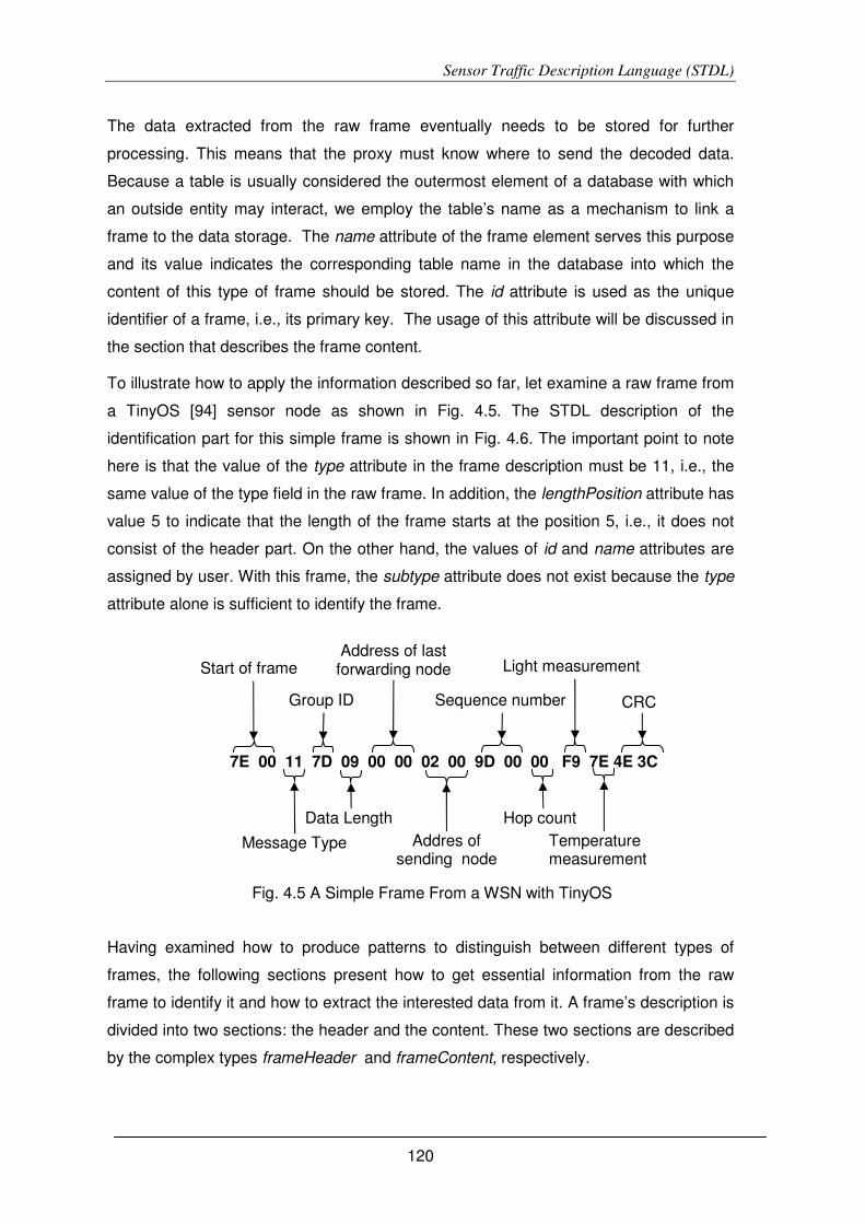
Sensor Traffic Description Language (STDL)
120
The data extracted from the raw frame eventually needs to be stored for further
processing. This means that the proxy must know where to send the decoded data.
Because a table is usually considered the outermost element of a database with which
an outside entity may interact, we employ the table’s name as a mechanism to link a
frame to the data storage. The name attribute of the frame element serves this purpose
and its value indicates the corresponding table name in the database into which the
content of this type of frame should be stored. The id attribute is used as the unique
identifier of a frame, i.e., its primary key. The usage of this attribute will be discussed in
the section that describes the frame content.
To illustrate how to apply the information described so far, let examine a raw frame from
a TinyOS [94] sensor node as shown in Fig. 4.5. The STDL description of the
identification part for this simple frame is shown in Fig. 4.6. The important point to note
here is that the value of the type attribute in the frame description must be 11, i.e., the
same value of the type field in the raw frame. In addition, the lengthPosition attribute has
value 5 to indicate that the length of the frame starts at the position 5, i.e., it does not
consist of the header part. On the other hand, the values of id and name attributes are
assigned by user. With this frame, the subtype attribute does not exist because the type
attribute alone is sufficient to identify the frame.
Having examined how to produce patterns to distinguish between different types of
frames, the following sections present how to get essential information from the raw
frame to identify it and how to extract the interested data from it. A frame’s description is
divided into two sections: the header and the content. These two sections are described
by the complex types frameHeader and frameContent, respectively.
7E 00 11 7D 09 00 00 02 00 9D 00 00 F9 7E 4E 3C
Start of frame
Message Type
Group ID
Data Length
Address of last forwarding node
Addres of sending node
Sequence number
Hop count
Light measurement
Temperature measurement
CRC
Fig. 4.5 A Simple Frame From a WSN with TinyOS

Sensor Traffic Description Language (STDL)
121
4.3.4 The Frame Header Specification
The objective of frame header is to help the STDL engine to extract the specific
information from an instance frame to search for its description, i.e., associate a raw
frame with its description. As mentioned in previous sections, a raw frame can be
specified uniquely by a type and an optional subtype. The STDL header section of a
frame specification dictates how the above fields are retrieved from a raw frame. It is
worth noting that the header specification is not used to describe the real header of the
frame but its main purpose is to get enough information to uniquely identify the
description of a particular raw frame.
As shown in Fig. 4.7, one of the required elements of a frame header is the
startOfFrame, which is a unique sequence of bits at the beginning of the frame. This
element is useful to deal with the problem of heterogeneity and diversity of frames in
WSNs because different sensor networks use different start of frame sequences. The
content of this element can be a sequence of bits or a list of hexadecimal numbers in the
form of 0xnn ... 0xnn. It also has a numberOfBit attribute which specifies the number of
bits of this field. In order to constrain the startOfFrame to contain only the sequence of
bits or a list of hexa decimal value, the simple types are defined as shown in Fig. 4.8.
The first simple type name binaryOrHexa uses union element to indicate that its value is
either of the type hexaDecimalList or binaryNumber. These two simple types employ the
pattern technique to restrict their possible values to a list of hexadecimal number a
binary string, respectively.
<?xml version=“1.0“ ?>
<frames>
<frame id=”1” name=”light_temperature”
type=“11“ length=“0“ lengthPosition=“5“>
…
</frame>
…
</frames>
Fig. 4.6 STDL for a Part of a Simple Frame

Sensor Traffic Description Language (STDL)
122
The next three elements typeField, subtypeField, and lengthField are used to specify
how to get the values of the type, the subtype, and the length fields from the raw frame,
respectively. The crucial point to note is that the engine must know how to extract the
data from the raw frame. As a result, these elements have the same structure, and each
one consists of four attributes: dataType, startPosition, numberOfBit and byteOrder.
The startPosition attribute specifies the position of the field in the raw frame. The
numberOfBit attribute indicates its length in bits. Both these attributes are restricted to
non-negative integers. The dataType attribute is used to indicate the type of the data.
Currently, STDL supports the following data types: string, uint8, int8, uint16, uint16,
uint32, int32, ulong, and long. The byteOrder attribute specifies the encoding method
and its values either ‘little_endian’ and ‘big_endian’ for little endian and big endian byte
order, respectively. By default, ’little endian’ is assumed.
Fig. 4.7 The Content Model of the Frame Header Description

Sensor Traffic Description Language (STDL)
123
Besides these above essential elements, the description of a frame’s header may also
comprise three optional elements: sender, destination and gateway. These elements are
included in the header part because they present in most of the frames. The purpose of
these elements, as implied by their names, is to describe the address of the original
transmitter, receiver and gateway devices, respectively. These elements have the same
structure as that of the previous three elements.
As an illustration, Fig. 4.9 shows the header’s specification for the raw frame in Fig. 4.5.
The elements of header section are specified inside the <header> tag. It is also
important to note that the subtypeField element does not exist in the header section
because in this case it is not necessary. With the information in the header, the STDL
engine knows how to get the needed information from the raw frame. For example:
suppose that the engine wants to get the value of the type field in raw frame. From the
typeField element in the header description, it knows that this field is situated at position
2 from beginning of the frame, and it has 1 byte. Combining these two pieces of
information, the engine obtains the value 17 (11 hexadecimal) from the raw frame. In
this case, the byteOrder attribute is not necessary because the value of this field has
only one byte.
<xsd:simpleType name="binaryOrHexa">
<xsd:union memberTypes="hexaDecimalList
binaryNumber"/>
</xsd:simpleType>
<xsd:simpleType name="hexaDecimalList">
<xsd:list>
<xsd:simpleType>
<xsd:restriction base="xsd:string">
<xsd:pattern value="0x[0-9A-F]{2}"/>
</xsd:restriction>
</xsd:simpleType>
</xsd:list>
</xsd:simpleType>
<xsd:simpleType name="binaryNumber">
<xsd:restriction base="xsd:string">
<xsd:pattern value="[01]+"/>
</xsd:restriction>
</xsd:simpleType>
Fig. 4.8 The Simple Type for a Sequence of bits or Hexadecimal

Sensor Traffic Description Language (STDL)
124
4.3.5 The Frame Content Specification
The objective of frame content specification is to specify what information is needed and
how to get the needed data from instance frames. It is noticeable that it is not necessary
to have a one to one mapping between the content of a raw frame and its specification.
This means that the content specification could include information from the header
section of a raw frame. Because the field type is a core data type that is extensively
used in the frame content description, the next subsection is dedicated to this data type.
4.3.5.1 The Field Type
The most important and useful aspect of STDL is how to help the engine to extract the
needed information from the raw frames and to give them some meaning. In order to
fulfill this requirement, the field data type is designed for describing the fields in a raw
frame. Each field is described by six attributes as shown in Fig. 4.10. The attributes
dataType, startPosition, numberOfBit and byteOrder have exactly the same meaning as
discussed in previous section. The other two attributes are used to add the semantics
for the described filed. Particularly, the name attribute is used name the described field,
which is used as a field name in a table in data storage. The unit attribute is a string that
indicates the measurement unit of the field’s content.
Fig. 4.9 The STDL Header Description for Simple Frame in Fig. 4.5
<?xml version=“1.0“ ?>
<frames>
<frame id=”1” name=”light_temperature”
type=“11“ length=“9“ lengthPosition=“5“>
<header>
<startOfFrame numberOfBit=”16”>0x7E 0x00</startOfFrame>
<typeField startPosition="2" numberOfBit="8"
dataType="uint8"/>
<lengthField startPosition="4" numberOfBit="8"
dataType="uint8"/>
<sender startPosition="7" numberOfBit="16"
dataType="uint16"/>
<destination startPosition="5" numberOfBit="16"
dataType="uint16"/>
</header>
…
</frame>
…
</frames>

Sensor Traffic Description Language (STDL)
125
As previously mentioned, the frames in WSNs could be divided into three main
categories. Consequently, there are also three types of the STDL content specification,
simpleFrame, dataTable, and complexFrame, as shown in Fig. 4.10.
4.3.5.2 Simple Frame Description
The simpleFrame type is used to describe the type of frames that merely consist of a list
of data fields. Each field of simple frame corresponds to a field of the raw frame and is
described by the field type discussed in previous section. As an illustration, Fig. 4.11
shows a description for the raw frame in Fig. 4.5. In this example, it is assumed that the
only needed information is the sending node identification, light and temperature.
Fig. 4.10 The Model of Frame Content Specification

Sensor Traffic Description Language (STDL)
126
Consequently, the content element of the frame description only comprises three fields:
senderId, light, and temperature, respectively.
Based on the frame description in Fig. 4.11, when receiving a raw frame having the
format as in Fig. 4.5, the STDL engine will extract only the sender identification, the
temperature, and the flight information from it. In addition, the extracted information will
be stored in the table name “light_temperature”, constrained by the attribute name of the
frame element, on the storage. Equally important, the “light_temperature” has three
fields for storing the extracted data: senderId, light, and temperature, constrained by the
name attribute of field elements.
4.3.5.3 Data Table Frame Description
The second type of frame is called data Table because its body contains a list of
repeated measurement of different types of data. This type of frame can be used to
describe the aggregated data in WSNs. One possible scenario for its usage is when a
sensor node buffers multiple samples before offloading data to the base station. Another
possible case is when the intermediate nodes combine their collected data with that
<?xml version=“1.0“ ?>
<frames>
<frame id=”1” name=”light_temperature”
type=“11“ length=“9“ lengthType=“0“>
<header>
<startOfFrame numberOfBit=”16”>0x7E 0x00</startOfFrame>
<typeField startPosition=”2” numberOfBit=”8”
dataType=”uint8”/>
<lengthField startPosition=”4” numberOfBit=”8”
dataType=”uint8”/>
</header>
<content>
<simpleFrame>
<field name=”senderId” dataType=”uint16”
startPosition=”7” numberOfBit=”16” unit=”none”/>
<field name=”light” dataType=”uint8”
startPosition=”12” numberOfBit=”8” unit=”lux”/>
<field name=”temperature” dataType=”int8”
startPosition=”13” numberOfBit=”8” unit=”F”/>
</simpleFrame>
</content>
</frame>
…
</frames>
Fig. 4.11 Frame Description of the Raw Frame in Fig. 4.5

Sensor Traffic Description Language (STDL)
127
received from other nodes into a single frame and then send it to the base station. The
dataTable element is used to specify such a data frame.
As shown in Fig. 4.10, the content of a dataTable frame are divided into two parts
described by nonRepeatedFields and repeatedFields elements. The former comprises a
list of fields that describe the information related to the repeated data in the raw frame
such as its start position (startPositionOfData) and its number of the repeated items
(dataLength). In addition, it also comprises a list of fields to be stored in the data storage
such as sender, time, etc. The later consists of a list of repeated fields in the data
portion. Each field of the raw frame is described by the field type. Fig. 4.12 and Fig.
4.13 are examples of data table frame and its description structure. However, because
this data table is contained in a complex frame, we will explain them all together in the
next section.
4.3.5.4 Complex Frame Description
Besides two fundamental types of frames, when working with real world sensor
networks, it happens to have a scenario where a frame may contain one or more simple
frames or data table frames. We deemed such frames as complex and described them
using the complexFrame element. Because the complex frame contains other frames, it
is necessary to describe other frames as regular frames and then refer to them in the
complex frame. Consequently, specifying a complex is rather simple. As shown in Fig.
4.10, it consists of a list of subframe elements which only has one attribute named
frameID. The frameID attribute refers to the id attribute of another frame described in the
same document. The list of subframe elements is optional, i.e., it may not appear in the
description of a complex frame. In this case, the complex can contain any frames
described in the STDL document. Additionally, there is also some additional information
to describe the general data for the frame. This information is specified using the
description element.
The relationship between frameID and id attributes of frame description is described by
the constraints of XSD [183]. Particularly, In order to make the id attribute unique, the
unique constraint, which specifies the value of a specific attribute of an element must be
unique among a set of elements, is utilized. In addition, the key constraint also applies to
the id attribute to make it a key. The keyref constraint is applied to the frameID attribute
to establish a link between its value and that of the key attribute of the frame elements.

Sensor Traffic Description Language (STDL)
128
The complete description of STDL in Extended Backus-Naur Form (EBNF) is described
in Appendix A.
To illustrate how to describe the last two types of frame, consider a raw frame as
showed in Fig. 4.12. This is a complex frame that contains data table frame used in a
sensor network developed by Eneida [186]. The example frame consists of three
repeated fields: temperature, humidity and voltage. The STDL description for this type
of frame is shown in Fig. 4.13.
This raw frame in Fig. 4.12 is a complex one because it contains another frame inside its
payload. As shown in Fig. 4.13, the inside frame is described by a structure frame
named “temp_hum_volt” and its id is 5. Its content is specified by the dataTable element
whose repeatedFields element has three sub-elements (temperature, humidity, and
voltage) for describing the repeated data fields in raw frame. The description of the
complex frame contains a sub-frame with the value of its frameId attribute is 5. This
means that this complex frame contains another frame having an id value of 5, i.e., the
data table frame mentioned above. Because the complex raw frame does not have a
field type to identify it, the type filed of the first inner frame is used instead.
46 52 41 4d 45 00 00 0D B5 41 54 01 00 00 00 01 39 9c 57 42 80 5a 65 01 00
Start of frame Start of
Subframe
Station
Date & Time
Device Length
Type subtype
Prioprity
E8 03 1B 00 17 2D DF 15 2E DE …
Number of Items One Entry
Start of Data
1st measurement
2nd measurement
Fig. 4.12 An Example of a Complex Frame Containing a Data Table

Sensor Traffic Description Language (STDL)
129
<frames>
<frame id=”5” name=”temp_hum_volt”
type=“101“ subType=”01” length=“0“ lengthposition=“0“>
<header>
<startOfFrame numberOfBit=”16”>0x41 0x54</startOfFrame>
<typeField startPosition=”13”
dataType=”uint8” numberOfBit=”8” />
<subTypeField startPosition=”14”
dataType=”uint8” numberOfBit=”8” />
<lengthField startPosition=”16”
dataType=”uing16” numberOfBit=”16”/>
</header>
<content>
<dataTable>
<nonRepeatedFields>
<startPositionOfData name=”startPosition”
dataType=”uint16” startPosition=”18” numberOfBit=”16”/>
<dataLength name=”numberOfItem” dataType=”uint16”
startPosition=”16” numberOfBit=”16”/>
<field name=”station” dataType=”uint18”
startPosition=”2” numberOfBit=”16”>
</nonRepeatedFields>
<repeatedFields>
<field name=”temperature” dataType=”int8”
startPosition=”0” numberOfBit=”8” unit=”C”/>
<field name=”humidity” dataType=”uint8”
startPosition=”1” numberOfBit=”8” unit=”%”/>
<field name=”voltage” dataType=”int8”
startPosition=”2” numberOfBit=”8” unit=”V”/>
</repeatedFields>
</dataTable>
</content>
</frame>
<!—Describe a complex frame --!>
<frame id=”10” name=”temp_hum_volt”
type=”65” length=”0” lengthPosition=”9”>
<header>
<startOfFrame numberOfBit=40”> 0x46 0x52 0x41 0x4d 0x45
</startOfFrame>
<typeField startPosition=”22” numberOfBit=”8”/>
<lengthField startPosition=”5”
dataType=”uint32” numberOfBit=”32”/>
</header>
<content>
<complexFrame>
<subFrame frameId=”5”/>
</complexFrame>
</content>
</frame>
…
</frames>
Fig. 4.13 STDL Description for the Content of the Raw Frame in Fig. 4.12

Sensor Traffic Description Language (STDL)
130
4.3.6 STDL Editor
To facilitate the creation of the specification of frame structure, a graphical STDL editor
was developed. This editor helps the users to manipulate the frame structure easily and
quickly. In addition, it eliminates the need to work directly with XML, which is tedious
and error-prone. More importantly, it is not necessary for the users to know the syntax of
STDL to create the frame specifications. Fig. 4.14, Fig. 4.15 and Fig. 4.16 show the
green shots of the main menu of the STDL editor, the frame header and the simple
frame content composers respectively.
Fig. 4.15 The Header Composer
Fig. 4.14 The Main Menu of STDL Editor

Sensor Traffic Description Language (STDL)
131
4.4 The STDL engine
Turning now to the question of how STDL can be used to make the proxy adaptable. As
described in previous sections, STDL is only a mean to describe the traffic of sensor
networks. Clearly, it is useless unless there is a tool to realize it. This is the place where
the STDL engine comes to take its role. It is the core part of the proxy. As shown in Fig.
4.3, the STDL document acts as the “brain” of the engine, guiding it through the
processing of a received raw frame.
Prior to explaining the details of the algorithms for analysis process of the raw frames, it
is important to understand the general model of the STDL engine. In order to make the
proxy more flexible and extensible, the event-based model is employed in the STDL
engine where an event is raised after the engine processes a raw data frame. Another
important point is that the engine employing JSON method [99] for encoding the
extracted data in the event’s message.
The engine comprises two main components: a parser and an analyzer. The parser
takes STDL document as its input, checks its syntax, and produces a list of frame
structures for using by the analyzer. The analyzer takes the raw frames as its inputs and
uses the corresponding frame description in the frame structure list to extract the
necessary data. The analyzer also accepts commands in form of JSON messages from
the Request Receiver component of the proxy and transforms them into the raw
packets to send to the sensor network. Fig. 4.17 shows the fundamental components
and workflows of the STDL engine.
Fig. 4.16 The Simple Frame Content Composer

Sensor Traffic Description Language (STDL)
132
The analysis process of a raw frame comprises two steps: (1) determining the frame
description; and (2) extracting data. The algorithm for this process is described in Fig.
4.18. In the first step, the frame description for the raw frame is searched by examining
every frame structure in the list and comparing its type and subtype (if applied) value to
those of the raw frame until a match is found. In the second step, the frame structure is
used as a blueprint to extract the needed data from the raw frame. It can be seen from
the algorithm shown in Fig. 4.18 that after determining the type of frame, the method for
extracting data is called to process the raw data. There are three different methods for
processing the raw frames corresponding to three types of frames (ExtractSimpleFrame
for simple frame; ExtractDataTableFrame for data table frame; and
ExtractComplexFrame for complex frame). The details of these methods are described
in Fig. 4.19, Fig. 4.20, and Fig. 4.21 respectively.
Perhaps processing the simple raw frame is the simple one. As described in Fig. 4.19,
this process comprises a loop through all fields of the frame structure. With every field,
its value is extracted from the raw frame. This value is combined with the field name
(i.e., the value of the name attribute of the field) to form a key-value pair separated by a
colon. All the extracted key-value pairs combined with the name of frame structure (i.e.,
the value of the name attribute of the frame structure) to form a JSON message. Finally,
this JSON message is sent as the data of the event raised by STDL engine.
Fig. 4.17 STDL Engine
Raw frames
STDL
Raise Event
STDL Parser
0111…1010
JSON message
1101…0010
JSON message
STDL Analyzer
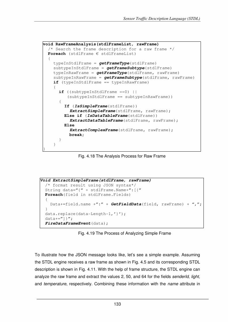
Sensor Traffic Description Language (STDL)
133
To illustrate how the JSON message looks like, let’s see a simple example. Assuming
the STDL engine receives a raw frame as shown in Fig. 4.5 and its corresponding STDL
description is shown in Fig. 4.11. With the help of frame structure, the STDL engine can
analyze the raw frame and extract the values 2, 50, and 64 for the fields senderId, light,
and temperature, respectively. Combining these information with the name attribute in
Void ExtractSimpleFrame(stdlFrame, rawFrame)
/* format result using JSON syntax*/
String data=“{“ + stdlFrame.Name+”:[{”
Foreach(field in stdlFrame.Fields)
{
Data+=field.name +”:” + GetFieldData(field, rawFrame) + “,”;
}
data.replace(data-Length-1,’}’);
data+=”]}”;
FireDataFrameEvent(data);
Fig. 4.19 The Process of Analyzing Simple Frame
void RawFrameAnalysis(stdlFrameList, rawFrame)
/* Search the frame description for a raw frame */
Foreach (stdlFrame € stdlFrameList)
{
typeInStdlFrame = getFrameType(stdlFrame)
subtypeInStdlFrame = getFrameSubtype(stdlFrame)
typeInRawFrame = getFrameType(stdlFrame, rawFrame)
subtypeInRawFrame = getFrameSubtype(stdlFrame, rawFrame)
if (typeInStdlFrame == typeInRawFrame)
{
if ((subtypeInStdlFrame ==0) ||
(subtypeInStdlFrame == subtypeInRawFrame))
{
If (IsSimpleFrame(stdlFrame))
ExtractSimpleFrame(stdlFrame, rawFrame);
Else if (IsDataTableFrame(stdlFrame))
ExtractDataTableFrame(stdlFrame, rawFrame);
Else
ExtractComplexFrame(stdlFrame, rawFrame);
break;
}
}
}
Fig. 4.18 The Analysis Process for Raw Frame

Sensor Traffic Description Language (STDL)
134
the frame structure (light_temperature), the STDL engine composes a JSON object
message as follows: {“ light_temperature:[{ “senderId”:2, “light”:50, “temperature”:64}]}. It
is worth noting that an array of objects is used even though there is only one object. The
reason is that by using an array of objects one message format can be used for all
events raised by the STDL engine.
The process of analyzing the data table frame is more complicated than that of the
simple frame. The reason is that the list of fields in raw frame is repeated. As a result,
the fields in the frame structure only describe the first instance of fields in raw frame. To
deal with this problem, the analysis process separates the data in the raw frame into
sub-frame and treats it individually. As shown in Fig. 4.20, the sub-frame is the part of
the data that contains one instance of the repeated fields.
It is not hard to process complex frames because it contains the frames of the other
types. Consequently, processing this type of frame is simple, extracting its sub-frames
and then calling the corresponding processing method. This process is described in Fig.
4.21.
Void ExtractDataTableFrame(stdlFrame, rawFrame)
String data=“{“ + stdlFrame.Name+”:[”
Int itemLen=GetItemLength(stdlFrame)
Byte[] item=new byte[itemLen]
Int curPosition = stdlFrame.startOfFirstyte;
While(curPosition + itemLen <= rawFrame.Length)
{
Item = copy(rawFrame, curPosition, itemLen)
Data+=ExtractListOfField(stdlFrame.Fields, item)+”,”
}
replace(data.Length-1,’]’)
Data+=’}’);
FireDataFrameEvent(data)
/** Extract a list of field value from a byte array **/
String ExtractListOfField(fields, bytes)
String data=“{“
Foreach(field in fields)
{
Data+=field.name +”:” + GetFieldData(field, bytes) + “,”
}
Data.replace(data.Length-1,’}’)
Return data
Fig. 4.20 The Process of Analyzing Data Table Frame

Sensor Traffic Description Language (STDL)
135
4.5 Prototype and Example Applications
4.5.1 Prototype
Besides the STDL and its engine, we developed a prototype for the proposed model.
The currently implemented proxy supports two methods to communicate with WSNs:
serial port and TCP/IP. For communication between the proxy and gateway the Web
service technology is employed. The encoding formats for communication between them
are JSON.
Similarly, the gateway middleware exposes the data and the functionalities of sensor
networks through a set of services with JSON. In addition, the middleware also supports
localization services based on RSSI. The localization services will be discussed in
chapter 5.
We tested the prototype with MICAz, TelosB [47] and EWS Eneida [186] sensor nodes.
The following section presents the example applications of the developed prototypes.
4.5.2 Example Applications
To illustrate how to use the proposed framework to integrate WSNs with other
application environments, we set up a testbed with three computers and two sensor
networks. Two computers act as proxies and collect data from the sensor networks; and
the other one acts as the gateway. The communication between sensor networks and
proxies is based on the serial port. In addition, FaceBook (FB) [181] social networking
platform and Second Life (SL [182]) virtual world were selected for testing integration.
Void ExtractComplexFrame(stdlFrame, rawFrame)
Int curPosition = 0;
STDLFrame stdlSubFrame
While(curPosition < rawFrame.Length)
{
subFrame = getSubFrame(rawFrame, stdlFrame,
stdlFrameList, out stdlSubFrame)
curPosition+=subFrame.Length
if (IsSimpleFrame(stdlSubFrame))
ExtractSimpleFrame(stdlSubFrame, subFrame)
Else
ExtractDataTableFrame(stdlSubFrame, subFrame)
}
Fig. 4.21 The Process of Analyzing Complex Frame

Sensor Traffic Description Language (STDL)
136
In the first application, the FB application Platform was employed as a front-end
application to display sensor data. The FB was chosen since it is the most common and
well-known social networking platform and it provides an API that allows for mashing up
with other environments. In this simple demonstration, we publish the temperature of the
monitored room in the wall of a FB account. This helps the account owner to instantly
know the temperature of the room in order to act appropriately in case it unexpectedly
changes. The result of this implementation is shown in Fig. 4.22.
The second application that we implemented based on our model was a mashup of
WSNs with the SL Virtual World. This application is similar to the first one but, instead of
displaying sensor data as plain text, we used virtual objects. In this simple application,
the temperature of the monitored target was represented by changing the color of an
object attached to an avatar. For example, if the temperature was between 10 and 19
degrees Celsius, the color of the corresponding object would become green and if the
temperature was greater or equal 50 degrees Celsius, the color would be red. Fig. 4.23
illustrates this process.
The above-mentioned applications show that sensor networks can become an integral
part of the virtual environments. The diversity of representation tools in 3D virtual worlds
and the sheer amount of users and social connections in social networks can open the
door towards new types of applications as well as promote the wide-spreading of sensor
networks and smart things and their integration with the Web.
Fig. 4.22 Publishing Sensor Data on FaceBook

Sensor Traffic Description Language (STDL)
137
Although our proposed model includes several layers, it is very fast and data coming
from the sensor nodes quickly reaches the client applications. For single hop
communications, it takes around 60 ms for data from the sensor nodes to reach the
proxy. From there, it takes approximately another 26 ms for data to reach the gateway
middleware and be available for the client applications. In the case of our mashup with
the Facebook [181] platform, it takes a total of 581 ms for data from physical
environments to be published and available to the users. During our tests, we could
sometimes get the data from the sensor nodes to be posted on Facebook as fast as in
246 ms. An important note is that this time includes the processing time at the proxy and
gateway.
The work in this chapter showed that a hybrid Proxy/Gateway is a suitable solution for
mashing up physical resources with virtual environments. It preserves the major
concepts of current research on sensor networks while providing an adaptable
infrastructure for seamless integration and interoperability of wireless sensors with
external applications.
Fig. 4.23 Displaying Temperature Using Object Attached to Avatar in SL

Sensor Traffic Description Language (STDL)
138
4.6 Conclusion
An extensible, interoperable and adaptable model for interoperating between WSNs and
application environments is an undeniable demand. The result of the research
presented in this chapter shows that it is possible to make the integration infrastructure
to be adaptable to the diversity of sensor networks by using STDL. In addition, the
event-based approach is adopted to make it easy for adding new components to the
framework. Furthermore, exposing data and functionalities of the WSNs as a set of web
services makes the interoperability process transparent to other application
environments.
The results of this study indicate that the framework can be adaptable to new
applications and protocols of WSNs. In addition, it is possible to treat WSNs as a plug-
and-play component of the Future Internet. This makes the development of applications
for sensor networks easier and more flexible. Developers can employ existing
applications to monitor, control, and visualize the sensor data and networks. This
approach is also a good method for mashing up the physical world information with
virtual worlds and other application environments.

Localization System for Wireless Sensor Networks
139
5 Localization System for Wireless Sensor Networks
Summary
5.1 Introduction
5.2 Application Scenarios
5.3 Localization System
5.4 Localization Methods
5.5 The Testbeds
5.6 Experimental Results
5.7 Conclusion
etermining the positions of sensor nodes, especially mobile nodes, in a WSN is
crucial for many applications. It helps to identify the location of the collected
data or of the node carriers such as the workers, patients or vehicles. It is a
critical requirement for supporting the timely right decisions. This chapter presents a
scalable localization system targeting controlled WSN in which a sensor network is
divided into multiple zones and (maybe overlapped) subzones. In addition, multiple
positioning methods were implemented and evaluated with real testbeds both in
laboratory and industrial environments. The localization engine is implemented as a
component of the gateway of the interoperability model presented in chapter 4.
D
Localization System for Wireless Sensor Networks
140
5.1 Introduction
With the ability to wirelessly connect a large number of tiny and low cost nodes, WSNs
have unlimited potential for useful applications. The nodes in a WSN can sense the
target environment (e.g., temperature, humidity, pressure, radiation, PH, etc.), do some
simple computation tasks and support wireless communications. Naturally, WSNs can
be applied in most fields including military, industrial, health-care, environment and
home monitoring. However, due to the constraints on the form, cost, and power
consumption, the sensor nodes have small memory, low commuting power, and limited
communication range. Consequently, there are many challenges related to the
application development, deployment, and management of this type of networks. Among
them, localization, i.e., determining the position of sensor nodes, is critical for many
applications because data are meaningless without knowing the location in which it was
obtained. In addition, the positions of the objects involved in the events are also
essential for many important applications such as searching, rescue, target tracking and
people health-care (e.g., workers in hazard environments, monitoring elderly or
Alzheimer).
Localization is the process of determining the position of devices, objects, things or
people in an area of interest. Location algorithms estimate the position of unknown
objects (i.e., sensor nodes) by using inter-sensor measurements such as Received
Signal Strength Indication (RSSI), Angle of Arrival (AoA), or propagation time. In
addition, it requires the knowledge of the positions of some sensor nodes or devices
called anchors, reference points or beacons. The localization problem has been studied
since 1960s resulting in the most successful location system, which is widely in use
today, GPS [23]. GPS based solutions are certainly a good choice for outdoors.
Therefore, one desirable option when considering localization for WSNs is to embed
GPS receiver in sensor nodes. TagSecure [187] is TagStone’s location aware personnel
tracking and safety management solution for hazardous environments. It is a GPS-
based solution for active tags, complemented with Radio Frequency Identification
(RFID) passive technology. Beyond the real-time GPS-based location, this location
system also keeps the information on the last gate (RFID Reader) crossed by a tag.
Because the GPS-based solution for sensor nodes is very high power consumption, the
work in [24] tried to reduce it by offloading GPS processing to the cloud. However, the
accuracy of this work is still low (35m). Hence, it is necessary to have alternative
solutions for localization in WSNs.

Localization System for Wireless Sensor Networks
141
One fundamental problem of localization in WSNs is that it is difficult to find an
appropriate measurement (e.g. distance) between the unknown position nodes and
anchors, considering the hardware and software restrictions, the requirements of
accuracy, feasibility and the cost. This problem is even more severe in noisy industrial
environments with a high degree of noise, interference and obstacles. As discussed in
chapter 2, ToA is not a suitable measurement method for WSNs because it requires a
very highly accurate clock and more complex algorithms to have the highly accurate
synchronization, i.e., in ns. The reason is that the communication in WSNs is mainly
very short distance while the travel speed of radio signal is very fast. Similarly, the
round-trip time method also requires a very highly accurate clock, and it is difficult to
calculate delay time at both sender and receiver. In addition, multiple messages
exchanged between the sensor node and several beacons are needed to obtain
information for estimating the position of the node. The AoA can produce more accurate
distance estimation. However, it is costly because of an array of antennae. In addition,
the accuracy of this method is severely affected by noise, interference, shadowing,
multipath, obstacles, and other factors. The combination of RF and the ultra-sound
reduces the complexity of antenna array. However, it requires the additional hardware,
which is costly and energy inefficient. In addition, it is also has the same problem as
those of AoA measurement method. Consequently, in spite of being unstable and
having a high variance, RSSI measurement method is, in most cases, the only choice
because of its availability.
The localization system presented in this chapter is based on the empirical
measurement of the RSSI between the sensor nodes and the anchors. In addition, it
includes the mechanisms for dealing with large-scale sensor networks while maintaining
the performance of location estimate process. The implemented location system was
evaluated in both laboratory and real critical industrial environment, the Soporcel paper
mill of Portugal [188].
5.2 Related Work
The location algorithms for WSNs can be divided into two broad classes: one for ad-hoc
(static or semi-static) sensor networks; and the other for controlled sensor networks. The
former is based on the assumption that the nodes in WSNs are deployed randomly into
the field and they rarely moved after deployment. In this case, the sensor network is
almost static except when the nodes die or are added. The latter class is applied for the
sensor networks that are carefully designed, using engineering methods. It is worth
Localization System for Wireless Sensor Networks
142
noting that a controlled sensor network comprises two main parts: the
infrastructure and the mobile nodes. The infrastructure is usually well designed and
includes a set of nodes with fixed known positions called anchors or beacons. On the
other hand, the mobile nodes are usually attached to workers, patients, or vehicles to
monitor the target environments or subjects. Consequently, determining the locations of
these mobile nodes is essential for many types of applications. Because our
localization system targets the controlled sensor networks, we focus our discussion
on the localization approaches for this type of WSNs.
Perhaps the simplest algorithm to estimate the position of a sensor node is based on the
“closest beacon” principle, i.e., the position of the node is the same as that of the closest
anchor based on a measurement, e.g., RSSI. For example, if the measurement is RSSI
then the position of the mobile node is also the position of the beacon that has the
strongest signal strength. Active Badge [25], Cricket [26], and Identec [27] are
examples of the positioning systems that employed this method. The advantage of this
method is that it is very simple to implement. However, it only provides relative location
such as in which room the node resides.
Another simple method is centroid algorithm [28] which computes the position of a
mobile node by averaging the coordinates of involved anchors, i.e., anchors in the range
of the node. In this method, the position of an unknown position node is determined by
the arithmetic mean of the coordinates of all the beacons in its communication range.
Similar to proximity method, this technique can only provide the relative location. In
addition, it returns the same position for nodes that are in the range of the same set of
anchors.
The second group of localization methods is based on the exploiting of the geometric
characteristics of triangles, circles, spheres or hyperbolae to estimate the position of the
unknown position nodes. In this approach, the localization problem is expressed as a
system of n equations (e.g., circles, spheres, or hyperbolae). As a result, the
position of a node is the solution of the equation system. Depending on the type of
measurement the methods in this approach could be divided into two groups:
lateration and angulation. Lateration method uses the distance measurement between
a device and several anchors to model the problem as a system of circular (2D) or
sphere (3D) equations, and when the number of equations is equal to 3 then it is also
known as trilateration. With this method, the measurement method could be ToA,
Round-trip Time of Flight or RSSI. However, because of the errors in measurement and
estimation, the intersection of circles or spheres may not result in a single point but an

Localization System for Wireless Sensor Networks
143
area; or in some cases, it does not intersect at all. Consequently, instead of solving the
system of equations, the linear or non-linear least square method [29], [30] is usually
used. GPS [23] is the most well-known public localization service employs this
algorithm. In addition, Bat [34] is the example of the lateration based location system for
sensor networks. The accuracy of this system is in the range of centimeters. However,
the use of a combination of ultrasound and RF makes this system more costly. In
addition, it is very susceptible to noise, obstacles, and non-LOS environments. The
recent work in [24] proposed a low power GPS-based solution for sensor nodes. This
work tried to reduce power consumption for sensor nodes by only getting the raw signals
from satellites and then forwarding them to the location service on the cloud for the
offline computation. The position of a node is computed by combining the information
from the raw signals obtained by the node itself and other sources. The current accuracy
of this system is still low (35m) [24].
In cases where the distances cannot be directly measured or estimated but instead the
differences of the arrival times of the signal at different anchors, a system of hyperbolic
equations can be formed and used to estimate the location of the node. One method for
finding the solution for the intersection of hyperbolas is to linearize the equations
through the use of Taylor-series expansion and to solve it using the iterative algorithm
[141]. Another method is to use correlation techniques with the cross-correlation function
of the signals [142]. The main disadvantage of this method is that it requires that all
anchors must be precisely synchronized.
Similar to lateration, angulation also bases on a system of equations for the localization
problem. However, instead of using distance measurements, it uses the Angle of Arrival
(AoA) of the transmitted signal at several anchors. In 2D space, the location of the
object is computed by the intersection of a pairs of direction lines. In 3D space, it is
possible to use these techniques for localization if the measurement of azimuth is
available. Ubisense system [189] is a location system which employed AoA and Ultra-
Wideband (UWB) to estimate the location. The accuracy of this method is very good (in
rang of cm). However, its cost is high because it requires directional antennae. In
addition, its accuracy is also severely affected by noise, obstacles, and non-LOS
environments.
With regard to finding the best estimate for the localization problem that are expressed
as an over-determined system of equations, Kalman filter [122] can be used. Kalman
filter is a recursively optimization estimator and it is widely used in almost every fields
including localization. It employs the prior knowledge of noise characteristics to account

Localization System for Wireless Sensor Networks
144
for and filter out the noises. In fact, Kalman filter can be used as an optimal tool in
other localization methods such as lateration or angulation. The research in [31],
[32], [33] employs Kalman filters for localization of sensor nodes, and claimed that its
accuracy is very good (less than 1 meter). However, the testbeds in these
researches were too small to assure the reliability of the accuracy. In fact, in our
experiments with trilateration method using RSSI measurement, employing Kalman
filter, the location error is much higher because of the error and instability of distance
estimation using RSSI.
As it is difficult to find an appropriate, accurate and reliable method for measuring the
distances between the mobile nodes and anchors, recent studies try to employ
algorithms in machine learning field for localization problem for WSNs. The localization
methods in this group are also known as pattern matching or learning-based,
fingerprinting or scene analysis. The methods in this category comprise three main
phases: (1) feature(s) collection, (2) training, and (3) location estimation. The objective
of the first phase is to collect the necessary data from the deployment environment. The
most common measurement collected for localization is RSSI because it is available in
almost all wireless networks. In the second phase, the collected data are then used to
train the algorithms to create the model and/or the necessary parameters. The final
phase uses the model or parameters computed in the second phase to estimate the
location of the unknown position objects by matching the new measurements with the
created model. The first two phases are done offline, while the last one is carried out in
real time. There are several localization algorithms in this approach including K-Nearest
Neighbors (KNN), Probability-based, Artificial Neural Network (ANN), and Support
Vector Machine (SVM).
KNN [148] is a common algorithm in machine learning and data mining for classification.
To determine the class for a test object, the KNN works as follows. First, k records that
are similar to the test object, based on some measurement, are searched from the
training dataset. Then, the class of the test object is that of the majority of k selected
records. KNN can be used for estimating the location of unknown position nodes by first
searching the fingerprint dataset to find k records that are closest matched with the new
observed data according to a distance function, e.g., Euclidean distance. By averaging
the coordinates of these k records, then, an estimated position of the object is obtained.
We could use the distances as the weights when averaging the coordinates of k records;
and in this case it is called weighted KNN. RADAR [35], MoteTrack [38], and LADMARC

Localization System for Wireless Sensor Networks
145
[37] are examples of localization systems that employed KNN. With the RADAR system,
it is possible to achieve 90th percentile of location error around 5.97m.
MoteTrack [38] adds the distributed ability to the system, by implementing the
localization algorithm on the sensor nodes. In addition, to improve the accuracy and
robustness, it requires that the sensor nodes have to listen on multiple channels to
collect data from multiple power levels. As stated in the paper, the accuracy of this
system is very good: with data from 16 channels the 80th percentile of distance error is
lower than 1.6m and with data from one channel the 80th percentile of distance error is
3.5m. Although MoteTrack [38] achieved an impressive accuracy, there are several
problems with this approach. First, it requires the sensor nodes to wait a rather long
time in order to acquire enough data for computing its location. Thus, it is not
appropriate for highly moving nodes. Second, because the beacons have to continue to
broadcast messages on multiple channels and power levels, it has very high power
consumption. Third, because the localization algorithm is implemented on the sensor
nodes, it cannot apply for the large sensor network having hundred or thousand
anchors.
LANDMARC [37] is another KNN based location system. However, instead of manually
collecting data from the deployment environment, this system employs a set of
reference tags for this purpose. The main advantage of this approach is that the first
step, i.e., collect feature(s), is not needed. In addition, the training dataset is always
updated. With a testbed in which reference tags are positioned at distance 2m x 1m, the
LANDMARC [37] achieved the 50th percentile of location error is about 1m and the 75th
percentile of error is about 1.2m. However, in order to obtain good accuracy, a high
density of reference tags, e.g., one tag every two meters is required. The high density
of reference tags leads to the high interference and thus it severely affected the
performance of the system. Moreover, the cost of this system is also high and it is not
appropriate for use in many real environments.
Another machine learning method that can be used for localization is based on
probabilistic theory. This method is similar to KNN, but instead of using the distance to
measure the ”similarity” between the new observed data and the records in the
training dataset, the probability-based methods use the likelihood estimation to
determine the similarity between them. A common method is to use Bayes’ rule [149] to
calculate the probabilities that the new observed data matches the records in training
dataset. Horus [39], [150] was a probability-based location system for WLAN that had
the 90th percentile of errors was about 1.43m. However, in order to obtain this accuracy

Localization System for Wireless Sensor Networks
146
the density of Access Points (APs) is high (average 6 APs per location). In addition, it
requires multiple samples for each location estimate. Moreover, because the system is
implemented on the client devices, it may be not appropriate for sensor nodes.
Elnahrawy et al. [151] was another study on using probabilistic approach for localization
in WLAN. They proposed Area-Based probability (ABP) to estimate the area in which a
mobile node resides. In this study, the authors also characterized the limits of using
RSSI for localization. The results from this study showed that using the RSSI for
estimating location has an expected bound for performance with the median of
distance error is about 3m and the 97th percentile of distance error is 9.15m [151]. This
is a reasonable conclusion because of the high variance and instability of RSSI values.
It is interesting to note that the ANN, which is inspired on the operation of the human
brain, can be used to solve many real world problems in different domains, including
pattern recognition, classification and regression. ANNs can also be used to solve
the localization problem in WSNs as research done in [42], [44], [153], [154]. The
study in [42] used the Cricket sensors [26] in its experiments and showed that the
performance of the neural network based solutions were better than those of the Kalman
Filter [31]. However, the testbeds in this experiment was too small to evaluate the
performance of ANN-based localization. On the other hand, the experiments of the
study in [154] were only done using simulation, whose results are rarely trusted for
evaluating the accuracy of localization methods. A more practical study in [44]
showed that ANN based localization for WLAN achieved the 90th percentile of distance
error was less than 5.4m. The advantage of this method is that it is very fast to estimate
the location (online stage). However, the training stage takes very long time and needs
experienced professional or empirical study to choose the good structure for ANN. In
addition, it cannot work well if the training dataset has many non-separable records,
resulting in significantly reducing the accuracy.
SVMs, also called kernel machines, are “maximum margin methods that allow the model
to be written as a sum of the influences of a subset of training instances” [149]. In SVM
method, the model is a class of kernel functions; and the training process tries to find the
best parameters for the kernel functions to make the margin (i.e., the distance from the
function to the nearest records of a class) as large as possible. SVM can also be used
for localization in wireless network as shown in [44]. The work in this paper showed that
SVM achieved the 90th percentile of distance error was about 5.12m. In addition, with
the same environment, its performance was a little better than other learning based
methods (Weighted KNN: 5.16m; Bayesian: 5.61m; and NN: 5.40m) [44].

Localization System for Wireless Sensor Networks
147
Every solution has its own merits and drawbacks, making it appropriate for different
applications’ requirements. The proximity and centroid methods are simple (i.e., easy to
implement and low memory computation demand) but their accuracy is very low, i.e.,
they only give a relative location such as in which room the node is. Similarly, lateration
and angulation approach also have a low memory and computation requirements.
However, their localization accuracy is dependent on a high accuracy and reliability of
the measurements, which are very difficult to achieve in WSN. Consequently, these
approaches usually give a very low accuracy in WSNs with RSSI measurement. On the
other hand, the machine learning based methods are complex in implementation and
require high memory and computation demand. However, the significant point to note is
that learning based methods are appropriate for controlled WSNs and are more
accurate than the others.
In this work, we proposed and implemented a localization system that is able to adapt to
the growth of the sensor network. More important, we evaluated the localization
methods for controlled WSNs in real critical industrial environments in order to find the
most appropriate method(s). The next section presents the targeted application
scenarios for our localization system.
5.3 The Application Scenarios
This section presents the application scenarios for which the localization system is
designed. In critical environments such as refinery, chemical plant, paper mill, etc,
determining the position of people (e.g., workers) or moving devices is very important in
order to have instantaneously appropriate responses. In these environments, the sensor
nodes are attached to the humans or vehicles, to monitor people’s current health (e.g.,
heart rate or blood pressure), the environment conditions (e.g., temperature, humidity or
air pressure), as well as their positions. By experiential working in critical industrial
environments such as oil refinery, paper mill and chemical plant, we found that these
environments have a lot of obstacles. Fig. 5.1, a part of a refinery, is an example of
such an environment with machineries, tubes, and tanks present everywhere. For these
reasons, using GPS may not be a good choice due to its low accuracy or unfeasibility
when used in such a scenario with so many obstacles and interferences. In addition,
high power consumption and additional hardware costs also prevent using GPS in
sensor networks.
Although mobile devices and wireless networks are limited in the refineries, the noise
and interference still exists. Our study presented in [190] shows that whereas there are

Localization System for Wireless Sensor Networks
148
no other wireless networks that interfere with the IEEE 802.15.4 based WSNs within the
refinery, there is still a considerable amount of signal noise caused by several types of
machineries, pumps, etc., that operate 24h a day. In addition, the effects of noise are
different between radio channels. Moreover, the noise and interference severely affect
the performance of the IEEE 802.15.4 based sensor networks in terms of delay and
packet loss as shown in [191]. Consequently it is necessary to have a suitable
localization for such scenarios. This means that the localization solution should work
well in noisy environments with a lot of obstacles, but with low power consumption.
It is important to note that in these application scenarios the mobile nodes do not usually
care about their own positions but the monitoring or controlling applications (e.g., the
Supervisory Control and Data Acquisition - SCADA) have to somehow locate the
position of these mobile nodes. This means that the position can be calculated by the
mobile nodes or by a central server, depending on which place is more appropriate.
However, in the case where the location is estimated by the mobile node itself, this
information has to be sent to the central servers, which host SCADA software, for further
processing. In our approach, to reduce the power consumption as well as the
computation burden of the sensor nodes, we decided to develop a central localization
system in which the positions of mobile nodes are estimated. The proposed localization
system implements multiple localization methods in order to allow users to select the
Fig. 5.1 A Typical Part of an Oil Refinery

Localization System for Wireless Sensor Networks
149
most appropriate one for a specific deployment environment. The next section presents
the proposed model.
5.4 Scalable Localization System
In order to create a positioning system that can respond to a large number of
concurrently requests, we employed a multi-layered software architecture for the
localization system. In addition, we also use the service-oriented principles for the
system, i.e., the communication between layers is based on web services. The general
model of the system is described in the following sub-section.
5.4.1 General Model of the System
The general model of the system is described in chapter 4 and this section only briefly
summarizes it. The main goal of this model is to provide a method for exposing the data
and functionalities of sensor networks and to allow an easy interoperability between the
WSNs and external environments including enterprise applications, web 2.0, virtual
worlds (e.g., Second Life [182]), and other applications. In addition, the model should be
also flexible enough to easily add infrastructure services (e.g., localization and mobility)
for WSNs. Moreover, it should be also scalable to apply for large sensor networks.
Consequently, we adopted a multi-layered architecture for the software system. As
shown in Fig. 4.1 in chapter 4, the model employs the proxies and gateways as the
mediate layers for interoperability between sensor networks and the applications that
monitor and control them. To support the scalability for sensor networks, there may be
more than one proxy associated with one gateway. Moreover, there can be more than
one gateway in the system. The details of these two components are described in
chapter 4. This section only discusses how they support for realizing localization
function.
The gateway, also called web service gateway, hosts localization engine, which
implements the localization algorithms. The localization engine accepts the localization
requests from the proxies, computes the position of the unknown position nodes, and
returns the results back to the proxies. More important, the location results are also
stored on the storage on the gateway (or a database server) for use by other
applications such as the visual application or SCADA via a web service interface. The
main advantage of the web service gateway is that it isolates the services from their
consumers. In addition, any changes to the middleware will not affect the applications
consuming the services provided that its interfaces are kept intact. Moreover, the

Localization System for Wireless Sensor Networks
150
security mechanisms such as authentication, authorization, and encryption can be
implemented at the gateway.
The proxy is responsible for obtaining, analyzing and forwarding the data from the
sensor network to the gateway. As discussed in previous chapter, the proxy is designed
to use an event-based principle, i.e., developers can register the listeners that capture
events of interest that happen in the network to add new component. In particular, to
support localization, the Localization Requester component registers to the ”data frame
arrival” event of the proxy to get the data from the sensor nodes. When having enough
data for a location request, it will compose the request and send it to the localization
engine on the gateway. This event-based model allows the system to be easily
extensible.
In order to make the seamless interoperability between the layers, web services are
employed in our software system. This means that the communication between proxies
and the gateway, as well as the communication between the gateway and users’
application, are based on web services. However, to reduce unnecessary overhead, the
communication between the sensor networks and proxy is serial port or IP based.
5.4.2 Localization Middleware
The localization middleware comprises several localization methods to estimate the
position of the sensor nodes when requested with appropriate data. The general
components of the location engine are shown in Fig. 5.2. As shown in this figure,
besides a list of implemented localization algorithms, the localization middleware also
includes methods for the proxies to request the positioning service. When receiving a
request, the localization engine will use the provided data, the model or training dataset,
and a localization algorithm to estimate the position of the node in the request. The
resultant position is then sent back to the proxy and stored in the database of the
gateway at the same time.
The position results stored on the gateway can be accessed and used by the monitoring
and controlling software or other applications. There are two methods for applications to
get location data from the gateway: polling and publisher-subscriber model. For the
former method, the applications periodically send request to the gateway to get the last
location data, while for the latter, the application subscribes the location request to the
gateway and when there is a new location result the location engine will raise an event

Localization System for Wireless Sensor Networks
151
to inform the application about the new data. All of these functionalities are provided by
the gateway via web service interfaces.
5.4.3 Localization Methods
In order to be able to evaluate and select the appropriate method for different sensor
networks, we implemented the following localization methods: Lateration, KNN [148],
Probability-based (Bayesian theorem) [149] and Kalman filter [122] over probability-
based. In the following discussion, RSSI measurement is used as the main input for our
localization methods because it is available in almost all WSNs and our current location
methods are also based on it. In addition, for the machine learning based methods, it is
assumed that the training dataset of the deployment environment is already collected.
The first algorithm implemented in our localization engine was Lateration. This algorithm
comprises two steps: (1) measuring or estimating the distance between a tag and some
anchors; and (2) computing the position of the tag using the intersection of circles or
spheres based on the measured (or estimated) distances obtained in step 1. Newton’s
method for nonlinear least square [29] was implemented in the location engine to solve
the over-determined system of equations to obtain an estimation of the position of the
unknown nodes. In addition, in order to estimate the distance from a tag to an anchor,
we also implemented several methods for converting RSSI value to distance. The
details of these conversion methods are presented in following section.
The second localization method implemented is KNN, which is based on the
principle “ similar input will have similar output”. This method is called lazy learning
algorithm because the training dataset is used as is. In this approach, the KNN algorithm
uses the observed RSSI vector (a list of pairs of anchor and RSSI value) to search for
Location Data Event Location Data service
event
Lateration KNN Probability-Based
Kalman Filter Over
Probability-Based
Localization Service
Fig. 5.2 Localization Middleware
Localization Methods
Localization System for Wireless Sensor Networks
152
k “closest” records in the training dataset according to some distance
measurement (e.g., mean square errors of Euclidean distance). Then, the position of
the unknown position node is computed by averaging the coordinates of these k
records. In addition, the distances can be used as the weights when computing the
average of coordinates; and KNN becomes the weighted KNN.
The third localization algorithm we implemented is based on the Bayesian decision
theory [149] and it is called Probability-based. Instead of finding K-nearest records
using the Euclidean distance, as KNN does, the Bayesian theorem is used to calculate
the probability of the entries in the training set, in order to find k highest probability
records for the observed RSSI vector. Then, the location of the unknown node is the
(weighted) average of the coordinates of the k highest probability records.
The final localization method implemented in our localization engine is Kalman filter
[122] over probability-based. In this implementation we combined two algorithms: (1)
Probability-Based; and (2) Kalman filter. This method first estimates the position of a
node using the probability-based method mentioned previously. Then the resultant
position is used as input for the Kalman filter. Because we do not have a rigorous
mathematical model for this case, we assume that the estimation of the current position
is linearly related to previous estimated position, the current measurement and the
noise. Consequently, our model for Kalman filter is as follows:
Y�4 = �4�� + +4���4 = �4 + 34�� Z In which, zk is the position given by the probability-based method; xk is the tag position;
wk-1 and vk-1 are the process and measurement noise, respectively.
In our implementation, we assumed that the noise does not change over time. This
means that wk=wk-1=…=w1 and vk=vk-1=…=v1. Consequently, the process and
measurement noise matrixes were computed once and based on the errors of the
probability-based method.
5.4.4 Scalable Mechanisms
The above localization methods work well for sensor networks with limited number of
anchors. However, they will have some problems when used with sensor networks that
have a large number of anchors and cover a large region. First, the training dataset
significantly grows if each record comprises all the anchors of the entire sensor network.
In addition, the location estimation process is slower when the training dataset becomes
Localization System for Wireless Sensor Networks
153
larger. Moreover, because the range of each anchor is limited, only a small number of
anchors have useful values in each record of the training dataset. As a result, it wastes
a lot of system resources, i.e., memory and computation, and affects the performance of
the location system. The problems are more severe for the KNN and Probability-based
methods. The reason is that these two methods belong to the lazy machine learning
algorithm type, i.e., instead of creating the model from the training dataset these
algorithms use it as is during estimation process. Therefore, reducing the size of the
training dataset used in position estimate process is one way to improve the
performance of the location system. However, if we do this by taking fewer
measurement positions, then the accuracy will be reduced. Consequently, we have to
keep taking the same number of measurements as well as the interpolation but
somehow to reduce the number of records used in the estimation process.
One possible method is to divide the entire network into different non-overlapped zones
which in turn is further divided into smaller subzones. A zone is a physically separated
area such as a site, a building, or a floor in a building. The objective of subzone is to
improve the performance and the estimation for each request only works on the dataset
of the subzone. In order to determine the subzone to be used on the estimate process,
each subzone has one or more represented points. As a result, we come up with a two
steps localization process: (1) subzone determination (2) localization estimation on the
selected subzone.
Before being able to apply this two-step localization process method, some preparation
steps are needed. First, we have to define a set of zones sand subzones. Then, we
have to process the collected data to create the training dataset for each subzone.
These preparation steps need to be done only once. Dividing a WSN into zones is
simple because it is based only the physical separated area. For the subzones, there
are two possible methods: (1) beacon-based and (2) area-based. For the former
method, the subzones are determined based on a list of anchors. Consequently, each
subzone is represented by a list of unique beacons. In this case, to determine a
subzone for estimating the position of a node, the location system uses the
anchors’ ID from the input data. It is important to note that subzones may be
overlapped, i.e., they may cover common areas and thus have some common
anchors. Consequently, it is possible that the list of anchors in an input data belongs to
two or more subzones. In this case, the subzone with the greatest number of matched
anchors wins and a tie is broken by randomly choosing a zone.

Localization System for Wireless Sensor Networks
154
For the latter method, each zone is divided into smaller areas called subzones. The
division can be simply based on the size of the area or it can also be based on the
physical conditions such as obstacles, shapes, or terrains. It is important to note that the
subzones might have the same list of anchors. Consequently, it is necessary to have an
appropriate method to select the subzone. Our solution for this problem is to use the
representative record(s) for each subzone. This means that for every subzone we select
a position, e.g., at the centre of the subzone’s area, as the representative point. Then,
the data collected at the representative position serves as the representative record. It
is possible to have more than one representative record for each subzone by choosing
multiple representative positions. To select a subzone for a location estimate, the engine
computes the similarity (e.g., distance) between the input data and the representative
data of the subzones. The closest subzone is chosen to use for the second step, i.e., for
the localization process, which is the same as the one presented in previous section, but
with the subzone dataset.
The current implementation of our location system employs the second method to
organize the subzones, i.e., area-based. Fig. 5.4 shows an example of a simple
subzone division in which a subzone is an entire floor. However, in the real environment,
a subzone can be a part of a floor. With this division, the entire training data set will be
divided into multiple data sets (one data set for each subzone). The training data set for
each subzone is reduced and only comprises data collected in an area covered by the
corresponding subzone. By organizing training data this way, the performance of the
location estimate is significantly improved. In fact, the location computation time remains
the same regardless how large the sensor network is.
To further improve the accuracy as well as the performance, we employ a two-step
method in the selecting subzone process. In the first step, some readers with the
strongest RSSI values are used to limit the possible area of the tag. The result of this
step is a list of subzones which have the areas overlapped with the region limiting by the
position of these readers. In the second step, one subzone is selected by computing the
similarity between the new observed values and representations of the subzone list
selected in the first step.
It is important to note that the data collecting phase is the same as that applies to the
entire network. This process comprises three main steps. First, determining the
positions where data will be collected. Second, collecting feature(s) by putting the
sensor nodes at the chosen positions to get the signal strength and/or other data if
applicable. Finally, the collected data are processed to create a training dataset for

Localization System for Wireless Sensor Networks
155
using in the localization process. The next section presents our testbed environments
and the experimental results done with our localization system.
5.5 The Testbeds
This section presents testbeds that are used in the experiments. The objectives of the
testbeds are to evaluate and to compare the performance of different localization
methods.
5.5.1 Sensor Platform
Because industrial plants are characterized by having huge metal structures and pipes
everywhere, and some with concrete walls or platforms, the LOS communication cannot
be considered in this system. In order get more range in distance, and communication
robustness in such scenarios, the 433MHz based sensor networks are used. The
testbeds in these experiments used the sensor hardware developed by Eneida [186], an
engineering company specialized in Instrumentation, Energy and Communications and
dedicated to the process industries. The equipments used in our testbed include: (1) the
smart active tags (EWS µ433M and EWS µ433M1Ex), which broadcasts its own ID; (2)
the wireless communication devices (also called readers) (EWS G433M and EWS
G433M1Ex), which receive the data from the tags, obtain the RSSI, and forward them
to the gateway devices; and (3) the communication gateway devices (EWS GIP or
EWS GIPW), which accept the data from the readers and forward them to the central
servers for further processing. The gateway devices get messages through CAN bus
[192] or wireless, and then delivery them to the server via Ethernet or Wifi
communication [186].
The radio component of this sensor system is based on the CC1101 radio transceiver
from Texas Instruments (TI) [193]. This module is able to operate in the sub GHz ISM
bands of 433MHz, 866MHz, and 902MHz and has features like low power consumption,
automatic packet handling or serial asynchronous communication and channel hopping
capabilities. The communication stack used in this implementation was the SimpliciTI
from TI [193]. It is a royalty free stack and provides basic point to point or tree topology
networks. It has built in encryption capabilities (XTEA algorithm [194]) and provides a
MAC layer with Carrier Sense for medium access. One possible topology of this type of
sensor net work is depicted in Fig. 5.3. The communication between readers and the
gateway can also be wireless.

Localization System for Wireless Sensor Networks
156
5.5.2 Testbed Environments
To evaluate the performance of the location system with different environments, we set
up and did the experiments with two testbeds. The first one consists of two sites: the first
one is at the Instituto Pedro Nunes (IPN) building in which Eneida Company is situated
and the second one is at the fire department of Coimbra, Portugal which is about 300m
from the IPN building. The first location is a two-story building where readers were
deployed in both floors, creating two different zones. Consequently, the entire sensor
network is divided into 3 zones: zone 1 is located at the 1st floor of IPN, zone 2 is the
2nd floor of IPN building and zone 3 is the fire department. The layout of the test-bed
is shown in Fig. 5.4. In this scenario the localization system is implemented on one
server and placed at the 2nd floor of the IPN building.
Fig. 5.3 EWS Sensor Network Topology

Localization System for Wireless Sensor Networks
157
The second testbed was set up at the Soporcel [188] paper mill, Portugal. In this
experiment the test-bed was installed in the recovery boiler for power production
building. This is a very hazardous and critical environment. There were 11 readers
installed on the floor 4, 5, and 6 of the 18 story building. The area of each floor is about
990 square meters (33 m x 30 m).
5.6 Experimental Results
With the installed test-beds we did numerous experiments with different configurations
and objectives. The following sub-sections present the experimental results obtained
from both laboratory and real critical industrial environments, Soporcel [188] paper mill,
and the comparison of the performance between the different environments. Before
presenting the location methods, we did numerous analyses to find ways to improve the
accuracy and robustness of the location methods
Fig. 5.4 Testbed at IPN Building and Fire Department
Fire Department
ID 13
ID 10
ID 11
ID 12
Zone 3
ID 18
ID 8
ID 16
IPN 1st floor
Zone 1 Zone 2
ID 2
ID 7
ID 3
ID 5
Center server room
IPN 2nd floor

Localization System for Wireless Sensor Networks
158
5.6.1 RSSI Calibration
The lateration localization method requires the distances from the sensor node to
several anchors. In most cases, however, the only feasible measurement in a WSN is
the RSSI value. Thus, it is necessary to have a method to convert RSSI value to the
distance. In order to find a good correlation between RSSI value and distance, we
evaluated four possible conversion methods: (1) Mean RSSI value; (2) linear regression;
(3) Friis Transmission Equation [195]; and (4) kernel smoother algorithm [149].
In the first method, the correspondence between RSSI value and the distance is
computed using the arithmetic mean of the measured RSSI values at each distance.
The result of this computation is a mapping table of pairs of distance and RSSI value.
For the second method, we tried to find the values for the parameters a and b of the
straight line distance = a.rssi + b that fit the collected data with minimum errors. The
third method is to use the collected data to infer the values for the parameters of the
Friis transmission equation [195]:
�FF[ \]^� = − 10. _. `ab \� + *� => \ = 10�deefIW��.'
In which A is the absolute value of RSSI within 1m distance; the signal propagation
coefficient n shows the damping of the signal. Both parameters are determined
empirically.
The final method is called the kernel smoother [149], which uses nonparametric
regression to estimate the distance from RSSI value. Its principle is that close input (x)
will have close output g(x) value. Assuming that the training dataset is X = { xt, rt}, rt ϵ R,
this method can be expressed as follow.
b �� = ∑ g � − �hℎ ��h∑ g � − �hℎ �
In the equation h is the width and k is the kernel function. One common used kernel
function is the Gaussian kernel as follows [149].
g i� = 1√2k l m� G�n�o�po ; q = 0, l = 1
To evaluate these methods, the RSSI values at different distances are needed. In this
experiment, we collected RSSI values between a tag and a reader at different distances
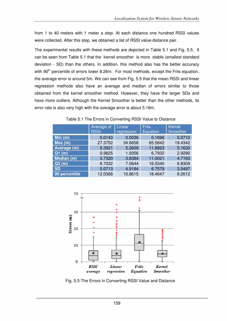
Localization System for Wireless Sensor Networks
159
from 1 to 40 meters with 1 meter a step. At each distance one hundred RSSI values
were collected. After this step, we obtained a list of RSSI value-distance pair.
The experimental results with these methods are depicted in Table 5.1 and Fig. 5.5. It
can be seen from Table 5.1 that the kernel smoother is more stable (smallest standard
deviation - SD) than the others. In addition, this method also has the better accuracy
with 90th percentile of errors lower 8.26m. For most methods, except the Friis equation,
the average error is around 5m. We can see from Fig. 5.5 that the mean RSSI and linear
regression methods also have an average and median of errors similar to those
obtained from the kernel smoother method. However, they have the larger SDs and
have more outliers. Although the Kernel Smoother is better than the other methods, its
error rate is also very high with the average error is about 5.16m.
Fig. 5.5 The Errors in Converting RSSI Value and Distance
Table 5.1 The Errors in Converting RSSI Value to Distance
Average of RSSI
Linear regression
Friis Equation
Kernel Smoother
Min (m) 0.0143 0.0036 0.1696 0.0710 Max (m) 27.3752 34.6658 65.5842 19.4342 Average (m) 5.3921 5.2609 11.8823 5.1630 Q1 (m) 0.9825 1.9356 6.7932 2.9290 Median (m) 3.7320 3.8384 11.0021 4.7163 Q3 (m) 6.7032 7.0644 16.5340 6.8309 SD 5.0713 4.9184 6.7579 3.5497 90 percentile (m)
12.0368 10.8615 18.4647 8.2612

Localization System for Wireless Sensor Networks
160
5.6.2 The Spread and Distribution of RSSI Values
Finding the spread of RSSI is also important because it provides information about how
stable (or unstable) the RSSI is. In addition, it is worth noting that the probability-based
localization methods assumed that the distribution of RSSI values is normal.
Consequently, it is necessary to have an empirical study to see whether or not this
assumption is acceptable. In order to evaluate the spread and distribution of RSSI
values, we put a tag and a reader at fixed positions and measured the RSSI values
received at the reader. To avoid the interference caused my people moving around, we
did the experiments during the night in a room with the door closed. We totally collected
58978 RSSI values. The histogram in Fig. 5.6 indicates that, in this case, the spread of
RSSI value, i.e., the range between the maximum and minimum, is 29.
In order to see whether or not the RSSI values from this experiment obey the normal
distribution, we also calculated the average and SD of the collected data. The red line in
Fig. 5.6 shows the graph of normal distribution using the computed average and SD
over the scaled histogram of the real data. Although these two graphs are not totally
matched with each other, the distribution of the RSSI values is approximate to the
normal distribution. This result allows us to use the normal distribution in the
probabilistic-based localization algorithm.
Another relevant point top note is that combining this result and that of previous section,
we can conclude that the RSSI values are unstable. The reasons for this conclusion are
that with a fixed position, the measured RSSI values have a very high range and large
SD.
Fig. 5.6 The Distribution of RSSI Values

Localization System for Wireless Sensor Networks
161
5.5.3 Training Dataset
In order to estimate the position of a node, the machine learning based localization
methods need to have a training dataset. The dataset consists of a list of records;
each comprises the features collected at a specific position in the deployment
environment. In addition, to compute the matching likelihood between a new
observed data and a record in the training dataset, the probabilistic methods need
SD of the RSSI of each anchor. Analyzing the collected data, we recognize that the
SDs for each anchor varies from position to position. Therefore, it is more appropriate
to use the SDs computed at each collected position in computing matching
likelihood. Consequently, each entry in the training dataset is a tuple with the following
information:
<x,y,z, rssiAvg1, rssiStd1,…, rssiAvgn, rssiStdn>
In which:
x, y, z are the coordinates of the position where the data is collected;
rssiAvgi is the average of RSSI values from the anchor ith;
rssiStdi is the SD of the RSSI values of anchor ith at position x, z, y.
Because collecting data is very time-consuming, we cannot collect the data in very fine-
grained positions (e.g., 1 or 2 square meters each). Therefore, we applied a method
similar to that used in [151], i.e., we collected RSSI values at the distance about 3-5
square meters and then did an interpolation to create a fine-grained dataset for training
the localization algorithms. To make the testing of the accuracy more reliable, we
independently collected two datasets: one for training and the other for testing. As an
example, the red points in the Fig. 5.4 are the positions in which the data were collected
for the first testbed. With the collected data being from 30 to 80 positions for each zone,
the interpolation process produced about more than 1000 entries for the training
dataset, each entry representing a point (or a tile) in a zone. The collected datasets
were used to evaluate the localization methods in the following sections.
5.6.4 Evaluating the Lateration Localization Methods
As previously discussed, the accuracy of lateration algorithm depends on the precision
of the distance measurement or estimate between the tag and the anchors. However,
the results obtained from the experiments showed that the conversion between RSSI
values and distance has a very high error (Table 5.1). In addition, it can be seen from

Localization System for Wireless Sensor Networks
162
Fig. 5.6 that the RSSI is also unstable, with a high variance. These factors affect the
accuracy of lateration method. In fact, by using the Kernel Smoother method for
conversion between RSSI value and distance, the lateration method produced a very
low accuracy. In addition, observing the results of this experiment, we saw that the error
in distance measurements has a significant effect on the error estimation of the height (z
coordinate). In most cases, the estimation error of z coordinate is unacceptable.
Furthermore, without taking into account the estimation error of z coordinate, the error of
this method is also very high; the majority of errors were greater than 10 meters.
Consequently, in the following sections this method will not be involved in the
evaluation.
5.6.5 Evaluating the Localization Methods with the Laboratory
Testbed
This section presents the experimental results of three localization methods (KNN,
probability-based and Kalman Filter over Probability-based) with the testbed installed at
IPN building. The distance errors of these localization algorithms are depicted in Table
5.2 and Fig. 5.7.
Comparing to lateration, the accuracy of these methods is significantly improved. As
shown in Table 5.2 , it is possible to obtain the average distance error less than 3.8m.
In addition, the Probability-based and Kalman filter over Probability-based methods
produce a better accuracy (lower average distance errors) and are more stable (smaller
standard deviation) than KNN. Comparing to KNN, it can be seen that the average
error of the probabilistic method are improved about 11.12% (from 3.79m to 3.37m).
Similarly, the average accuracy of Kalman filter over Probability-based method is also
Table 5.2 The Distance Errors of Localization Algorithms in Laboratory
Environment
KNN
Probability-Based
Kalman Filter Over Probability-Based
Min (cm) 6.64 0 6.02 Max (cm) 1809.87 1602.53 1456.09 Average (cm) 379.46 337.20 332.96 Median (cm) 231.31 199.92 205.99 75 Percentile (cm) 510.56 435.49 420.68 80 Percentile (cm) 609.24 534.56 508.64 SD (cm) 201.40 178.31 158.24

Localization System for Wireless Sensor Networks
163
better than KNN about 14.89% (3.79m and 3.33m, respectively). Equally important, as
shown in Fig. 5.7, the 80th percentile of distance errors is reduced from 6m (KNN) to
about 5m (other methods).
5.6.6 Evaluating the Localization Methods with the Testbed in
industrial Environment
To evaluate the performance of the implemented location algorithms in a real critical
industrial environment, we installed a testbed in a recovery boiler for power production
building, located in Soporcel paper mill [188]. With this testbed, we did numerous
experiments with different configurations and objectives. The Table 5.3 and Fig. 5.8
present the results of experiments with a testbed comprising 11 readers installed on 3
floors (4, 5, and 6) of this building.
Fig. 5.7 The Distance Errors of Localization Algorithms With IPN Testbed
Table 5.3 The Distance Errors of Localization Algorithms with the
Testbed installed at Soporcel Paper Mill
KNN
Probability-Based
Kalman Filter Over
Probability-Based Min (cm) 1.58 0 0 ax (cm) 2049.18 1968.72 1904.23 Average (cm) 449.15 431.98 434.31 Median (cm) 187.04 122.47 338.88 75 Percentile (cm) 753.27 755.99 718.63 80 Percentile (cm) 861.91 867.43 806.71 SD (cm) 251.77 257.45 225.51

Localization System for Wireless Sensor Networks
164
Comparing with the results of the experiments done at the IPN building, it can be seen
that the accuracy in this environment is significantly reduced. In particular, the average
distance error of KNN is increased from 3.79m to 4.49m (15.52%) and those of
Probability-based and Kalman Filter over Probability-based methods are increased
from 3.37m to 4.32m (21.94%) and from 3.23m to 4.34m (25.64%), respectively. There
are several possible explanations for this result. First, the second testbed was installed
on a very noisy environment with a lot of motors, pumps, and other machineries. In
addition, the obstacle and the heating from the recovery boiler may also affect the
stability of RSSI and thus the accuracy of the location estimate. Moreover, the position
of the readers is also a factor that influences the performance of the location system.
It is also important to note that when compared to KNN, in terms of location estimate
accuracy, the performance of the other two methods is also a little bit better. However,
the differences are not as substantial as those obtained in the first testbed.
With the collected data, we also analyze the accuracy of the location system at different
areas in the real environment. The objective of this study is to find out the positions that
had good accuracy and why they are better than the others. In this study, the floors 4, 5,
and 6 are divided into 9, 7, 7 subzones, respectively. From the results of the
experiments, we find out that among these 23 subzones, 9 of them (39.13%) have the
average distance errors less than 2.23 meters with 80th percentile of errors are less than
4.4 meters. Table 5.4 and Fig. 5.9 describe the location errors of these subzones.
By observing the locations of these best subzones, we recognize that all of them are
located in the boundaries of at least three readers. In addition, the communication
between the readers and the tag in these subzones is rather clear. This is not
Fig. 5.8 The Distance Errors of the Localization Algorithms at Soporcel

Localization System for Wireless Sensor Networks
165
necessarily a line of sight communication, but the obstacles between the reader and tag
are not too big. Moreover, the distance between the readers also contributes to the
accuracy, as in these best subzones the distance between readers is about 15 meters.
The implication of this study allows us to design and deploy a location system with
different levels of accuracy for different zones. For instance, we should deploy more
readers for the high critical zones and fewer readers for other less important zones.
From the results of our experiments and those of other authors, e.g., [151], we can
conclude that by using only RSSI values we cannot make more improvement on the
Fig. 5.9 The Distance Errors of the Best Subzones at Soporcel
Table 5.4 The Distance Errors of Best Subzones at Soporcel Testbed
subzone 1 2 3 4 5 6 7 8 9
Min 0 0 0 0 0 0 0 0 0
Average 207.50 116.42 41.76 131.65 202.31 222.56 143.10 218.10 193.89
median 17.98 19.60 0 16.90 19.07 45.91 5.85 16.31 28.51
75 Percentile 145.92 41.71 14.00 94.00 339.80 319.22 181.71 341.56 345.62
80 percentile 425.77 50.26 73.80 359.87 411.26 424.28 424.57 440.51 432.72
90 percentile 604.74 592.80 146.94 480.17 504.97 521.33 526.69 587.88 601.33
Max 1066.47 812.10 958.29 928.78 1037.63 1052.33 1094.45 1088.58 923.15
Std, Dev 178.94 113.38 75.05 109.16 134.63 139.10 122.36 179.87 143.52
Unit: cm

Localization System for Wireless Sensor Networks
166
accuracy of localization than those obtained in our experiments. The fundamental
problem is not from the localization algorithms but from measurements, i.e., instability of
the RSSI values. However, the accuracy and precision provided by KNN, probability-
based (Bayesian theory) and Kalman Filter over Probability-based localization methods,
are sufficient for many real world applications.
5.7 Summary
In this chapter, we present our model for localization system that can be applied for
large-scale sensor networks. The localization engine implements numerous localization
methods. We also did several experiments with two testbeds, one in the normal
environment, and the other in a critical industrial environment, to evaluate the accuracy
of the implemented localization methods.
The results from experiments show that RSSI values are unstable with high variance. As
a result, lateration is not good in terms of accuracy when using RSSI values as the only
measurement. On the other hand, pattern matching based methods such as KNN,
probability-based and Kalman Filter over Probability-based produce a sufficient
accuracy for many application scenarios. With these methods, it is possible to achieve a
mean error less than 4m and 80th percent of errors is less than 6m. More important, by
carefully engineering the positions of readers, it is possible to obtain an average
distance error of about 2.2m.

Conclusion and Future Work
167
6 Conclusion and Future work
Summary
6.1 Conclusion
6.2 Future Work
SNs have been being deployed for the real industrial environments,
especially critical ones such as refineries, industrial plants (e.g., chemical
processes, paper mills), and mining. Developers of WSNs for such
environments face numerous challenges in designing, developing, deploying, and
maintaining such as energy efficient protocols, reliable communication, localization, and
integration. This thesis aims at creating the infrastructure for facilitating the
development, deployment, and maintenance of WSNs in critical environments. In
particular, it deals with the reliable communication, integration, and localization problems
of sensor networks. The work in this thesis consists of three main separated but closely
related topics. The first topic is about reliability in communication at low level of the
network protocol stack, i.e., MAC layer. The second one targets at the infrastructure for
interoperability between physical and digital worlds. Especially, it focuses on the
adaptability issue for the diversity and heterogeneity of sensors and sensor systems.
The final topic is about the supporting service for locating the unknown position nodes in
controlled WSNs. This chapter summarizes the work done in this thesis, its main results
and some future work.
W

Conclusion and Future Work
168
6.1 Conclusion
The aim of the work in this thesis is to facilitate the development, deployment, and
maintenance of WSNs in critical and industrial environments. To achieve this, the
proposed solutions focused on three important areas of the WSNs: reliability,
integration, and localization. The proposed solutions were implemented and evaluated
using real testbeds installed in different environments. The following paragraphs
summarize the work done in the context of this thesis.
The first issue of concern was to study the characteristics of different channels of IEEE
802.15.4 compliant sensor networks. The motivation of this work was from the problem
we encountered when deploying the WSNs at Galp Energias refinery, Portugal. During
the deployment of WSNs, we found that this hazardous and noisy environment greatly
influenced our networks performance, e.g., when operating on a default channel
(channel 26), the sensor network sometimes stopped working. This issue brought to our
attention several questions: do the channels of IEEE 802.15.4 compliant sensor
networks have the same quality? How are they affected by factors such as interference
and noise? What is the quality of channels like in different environments? In order to
answer these questions, numerous empirical experiments were done with the testbeds
in different environments. The results showed that the quality of channels of IEEE
802.15.4 based sensor networks is different from place to place and it varies from time
to time. From these studies we also recognized that interference, from other wireless
networks, has significantly impacted on the performance of the communication
channels. Equally important, it is clear from the study at the oil refinery that noises from
machineries, pumps, etc., severely affects the quality of the radio channels.
Consequently, it is very difficult or even impossible to predict the quality of different
channels of IEEE 802.15.4 based sensor networks deployed in a specific environment
without an experimental study.
As noise and interference have severe impacts on the performance of WSNs and they
are present almost everywhere, it is necessary to have a mechanism for WSNs to
continue working in such environments. This means that the sensor networks can work
well in the environments in which there are other wireless networks and noise sources.
This problem is referred to as the coexistence problem and the potential mechanism to
deal with it is called cognitive radio (CR). However, fully employing CR for WSN may be
difficult or inefficient. In order to allow WSNs to reliably operate in noisy and interference
environments, we propose a MAC protocol named Dynamic MAC (DynMAC). This MAC

Conclusion and Future Work
169
protocol is based on CR principles to allow the network to dynamically select the best
channel during its operation time. The best channel is selected by the cooperating
between nodes in the networks. In addition, it also employs some mechanisms to
improve the resilience and reliability of the network including packet loss rate monitoring,
loss link detection, and channel rescanning.
A prototype of DynMAC based on the GinMAC [69] has been implemented. The current
version of DynMAC was evaluated on both simulations, i.e., COOJA [172], and real
testbed. The results from the testbed showed that it is very fast to establish the network
during the boot time. In addition, the normal nodes can easily and quickly scan the
channel of the network and join it. Moreover, the network can also switch to a better
channel if the current channel becomes worse for some reason, e.g., a new installed
wireless network interferes with the sensor network. Furthermore, the nodes in a
DynMAC-based WSN can detect loss link and reestablish the connection.
Another relevant point is that the sensed data from the sensor networks need to be
processed, presented and visualized by suitable tools to make them meaningful. To
facilitate the interoperation between WSNs and external environments, we propose a
proxy and gateway–based integration framework. In this framework, the data and
functionalities of the WSNs are exposed using REST-based web services. This model
allows sensed data to be easily accessed from the Internet, and to be able to be
mashed up with web environments. More important, STDL language proposed in this
thesis helps the integration framework adaptable with diversity and heterogeneity of
sensor networks. The data frames in sensor network are described using STDL in order
for the proxy to extract the needed information. Consequently, the framework can be
used for any sensor networks if the structure of the frames are known and described by
using STDL. A prototype of this framework was implemented and evaluated with sensor
networks that run the contikiOS [95], TinyOS [94] and SimplicitI [193]. In addition, its
interoperability was also tested by integrating WSNs with FaceBook [181] and
SecondLife [182].
It is worth noting that locating mobile bodies, e.g., workers, patients, children, etc, has
many potential applications, especially in critical and industrial environments. The
position information helps to monitor the workers working in hazard environments. In this
thesis, localization system with multiple algorithms was implemented. In addition,
mechanisms for the localization system to be able to apply for large-scale sensor
networks were proposed. Several experiments were done with two testbeds, one in the
normal environment, and the other in a critical industrial environment, to evaluate the

Conclusion and Future Work
170
accuracy of the implemented localization methods. The experimental results showed
that although the RSSI values are unstable, the learning based localization methods can
produce a sufficient accuracy for many application scenarios.
6.2 Future Work
This thesis has achieved some interesting results; however, there are still aspects that
need further investigation. The first one is the limitation of the DynMAC protocol.
Currently, its implementation is based on GinMAC [69]. This means that it has the same
scalability problem of GinMAC i.e., 25 nodes per tree. In addition, the experiments were
only done in the laboratory. As a future work, it is necessary to do experiments with
DynMAC in different environments to evaluate its performance as well as the ability to
adapt to different environments or conditions. In addition, it is useful to improve the
scalability when applying the mechanism used in DynMAC principles to other MAC such
as X-MAC or T-MAC.
Concerning the STDL, we need to investigate the formats of the data frame from other
sensor systems and operating systems for sensor networks to test its adaptable
capability. This help to find out the limitation of STDL and to improve it.
Another limitation is that the localization system is only tested on the testbeds with
maximum three zones and 16 anchors. It is important to test the positioning system with
a larger testbed. As a future work, we will develop a simulation system to evaluate the
scalability of the localization system. This simulation will help to estimate the appropriate
hardware configuration for real application environments.

References
171
References
[1] A. Sikora and V.F. Groza, "Coexistence of IEEE802.15.4 with other Systems in the
2.4 GHz-ISM-Band," in Proceedings of the IEEE Instrumentation and
Measurement Technology Conference, 2005. IMTC 2005, Ottawa, Ontario, 2005,
pp. 1786-1791.
[2] S. Pollin, I. Tan, B. Hodge, C. Chun, and A. Bahai, "Harmful Coexistence Between
802.15.4 and 802.11: A Measurement-based Study," in 3rd International
Conference on Cognitive Radio Oriented Wireless Networks and Communications,
2008. CrownCom 2008, Singapore, 2008, pp. 1-6.
[3] A. Bachir, M. Dohler, T. Watteyne, and K. K. Leung, "MAC Essentials for Wireless
Sensor Networks," IEEE Communications Surveys & Tutorials, vol. 12, no. 2, pp.
222-248, quarter 2010.
[4] IEEE Computer Society, "IEEE Recommended Practice for Information
technology- Local and metropolitan area networks- Specific requirements- Part
15.2: Coexistence of Wireless Personal Area Networks with Other Wireless
Devices Operating in Unlicensed Frequency Bands," IEEE Std 802.15.2™-
2003(R2009), pp. 0_1-115, August 2003.
[5] J. Marinho and E. Monteiro, "Cognitive radio: survey on communication protocols,
spectrum decision issues, and future research directions," Wireless Networks, vol.
18, no. 2, pp. 147-164, February 2011.
[6] D. Cavalcanti, S. Das, J. Wang, and K. Challapali, "Cognitive Radio Based
Wireless Sensor Networks," in Proceedings of 17th International Conference on
Computer Communications and Networks, 2008. ICCCN '08, St. Thomas, US
Virgin Islands, 2008, pp. 1-6.
[7] A. Dunkels, J. Alonso, T. Voigt, H. Ritter, and J. Schiller, "Connecting Wireless
Sensornets with TCP/IP Networks," in In Proceedings of the Second International
Conference on Wired/Wireless Internet Communications (WWIC2004), Frankfurt,
Germany, 2004, pp. 143-152.
[8] I.F. Akyildiz, W. Su, Y. Sankarasubramaniam, and E. Cayirci, "Wireless sensor

References
172
networks: a survey," Computer Networks, vol. 38, no. 4, pp. 393-422, March 2002.
[9] C. Intanagonwiwat, R. Govindan, and D. Estrin, "Directed Diffusion: A scalable and
robust communication paradigm for sensor networks," in Proceedings of the 6th
annual international conference on Mobile computing and networking, Boston,
Massachusetts, USA, 2000, pp. 56-67.
[10] K.A. Emara, M. Abdeen, and M. Hashem, "A gateway-based framework for
transparent interconnection between WSN and IP network," in The IEEE Region 8
Conference EUROCON, St.-Petersburg, Russia, 2009, pp. 1775-1780.
[11] J.H. Kim, D.H. Kim, H.Y. Kwak, and Y.C. Byun, "Address Internetworking between
WSNs and Internet supporting Web Services," in Proceedings of the 2007
International Conference on Multimedia and Ubiquitous Engineering, Seoul, Korea,
2007, pp. 232-240.
[12] L. Shu, J. Cho, S. Lee, M. Hauswirth, and Z. Zhang, "Vip bridge: Leading
ubiquitous sensor networks to the next generation," Journal of Internet Technology
(JIT), vol. 8, no. 3, pp. 1-13, July 2007.
[13] K. Aberer, M. Hauswirth, and A. Salehi, "Infrastructure for Data Processing in
Large-Scale Interconnected Sensor Networks," in Eighth International Conference
on Conference on Mobile Data Management, Mannheim, Germany, 2007, pp. 198
-205.
[14] A. Dunkels, "Full TCP/IP for 8-bit architectures," in Proceedings of the 1st
international conference on Mobile systems, applications and services (MobiSys
'03), San Francisco, California, 2003, pp. 85-98.
[15] J. Hui, D. Culler, and S. Chakrabarti, "6LoWPAN: Incorporating IEEE 802.15.4 into
the IP architecture – Internet Protocol for Smart Objects (IPSO) Alliance.," IPSO
Alliance, White paper #3, 2009.
[16] J. W. Hui and D. E. Culler, "IPv6 in Low-Power Wireless Networks," Proceedings
of the IEEE, vol. 98, no. 11, pp. 1865-1878, September 2010.
[17] B. Priyantha, A. Kansal, M. Goraczko, and F. Zhao, "Tiny web services for sensor
device in-teroperability.," in In Proceedings of the IEEE 7th international
conference on Information processing in sensor networks, IPSN '08, Washington,
DC, USA., 2009, pp. 567-568.

References
173
[18] S. Dawson-Haggerty, X. Jiang, G. Tolle, J. Ortiz, and D. Culler, "sMAP — a Simple
Measurement and Actuation Profile for Physical Information," in Proceedings of the
Eighth ACM Conference on Embedded Networked Sensor Systems (SenSys '10),
Zurich, Switzerland, 2010, pp. 197-210.
[19] D. Guinard and V. Trifa, "Towards the Web of Things: Web Mashups for
Embedded Devices," in Workshop on Mashups, Enterprise Mashups and
Lightweight Composition on the Web (MEM 2009), in proceedings of WWW
(International World Wide Web Conferences), Madrid, Spain, 2009.
[20] Z. Shelby, K. Hartke, and C. Bormann, Constrained Application Protocol (CoAP)
draft-ietf-core-coap-18, 2013, https://datatracker.ietf.org/doc/draft-ietf-core-coap/.
[21] A. Dunkels, T. Voigt, and J. Alonso, "Making tcp/ip viable for wirelesssensor
networks," in In Proceedings of the First European Workshop on Wireless,
Swedish Institute of Computer Science, Sweden, 2004.
[22] R. Roman, J. Lopez, and C. Alcaraz, "Do Wireless Sensor Networks Need to be
Completely Integrated into the Internet?," in Future Internet of People, Things and
Services (IoPTS) eco-Systems, Brussels, 2009.
[23] A. El-Rabbany, Introduction to GPS: The Global Positioning System, 2nd ed.:
Artech House, 2006.
[24] J. Liu et al., "Energy Efficient GPS Sensing with Cloud Offloading," in 10th ACM
Conference on Embedded Networked Sensor Systems (SenSys 2012), Toronto,
2012, pp. 85-98.
[25] R. Want, A. Hopper, V. Falcão, and J. Gibbons, "The active badge location
system," ACM Transactions on Information Systems (TOIS), vol. 10, no. 1, pp. 91-
102, January 1992.
[26] N.B. Priyantha, A. Chakraborty, and H. Balakrishnan, "The Cricket Location-
Support System," in Proceedings of the 6th annual international conference on
Mobile computing and networking, Boston, MA, USA, 2000, pp. 32-43.
[27] Identec Solutions. (2013, March) Innovative Wireless Sensor Network Enables
Powerful Business Intelligence. [Online]. http://www.identecsolutions.com
[28] Y.C. Cheng, Y. Chawathe, A. LaMarca, and J. Krumm, "Accuracy characterization
for metropolitan-scale Wi-Fi localization," in Proceedings of the 3rd international

References
174
conference on Mobile systems, applications, and services (MobiSys '05), New
York, NY, USA, 2005, pp. 233-245.
[29] A. Bjõrck, Numerical Method for Least Squares Problems, 1st ed. Philadelphia,
America: SIAM: Society for Industrial and Applied Mathematics, 1996.
[30] W. Hereman and W. S. Murphy, "Determination of a position in three dimensions
using trilaterationand approximate distances.," Department of Mathematical and
Computer Sciences, Colorado School of Mines, Golden, Colorado, Technical
Report 1995.
[31] A. Shareef and Y. Zhu, "Localization Using Extended Kalman Filters in Wireless
Sensor Networks," in Kalman Filter Recent Advances and Applications, V. M.
Moreno and A. Pigazo, Eds. Rijeka, Crotia: In-Teh, 2009, ch. 13, pp. 297-320.
[32] M. A. Caceres, F. Sottile, and M.A. Spirito, "Adaptive Location Tracking by Kalman
Filter in Wireless Sensor Networks," in IEEE International Conference on Wireless
and Mobile Computing, Networking and Communications, Marrakech, Morocco,
2009, pp. 123-128.
[33] C. Rohrig and M. Muller, "Localization of Sensor Nodes in a Wireless Sensor
Network Using the nanoLOC TRX Transceiver," in The IEEE 69th in Vehicular
Technology Conference, 2009. VTC Spring 2009., Barcelona, 2009, pp. 1-5.
[34] A. Harter, A. Hopper, P. Steggles, A. Ward, and P. Webster, "The anatomy of a
context-aware application," Wireless Networks, vol. 8, no. 2/3, pp. 187-197, March-
May 2002.
[35] P. Bahl and V. N. Padmanabhan, "RADAR: An in-building RF-based userlocation
and tracking system," in Proceedings of Nineteenth Annual Joint Conference of the
IEEE Computer and Communications Societies, vol. 2, Tel Aviv , 2000, pp. 775–
784.
[36] J. Hightower, G. Borriello, and R. Want, "SpotON: An Indoor 3D Location Sensing
Technology Based on RF Signal Strength," University of Washington , Seattle,
Technical Report 2000-02-02, 2000.
[37] L.M. Ni, L. Yunhao, Yiu C.L., and A.P. Patil, "LANDMARC: indoor location sensing
using active RFID," in The First IEEE International Conference on Pervasive
Computing and Communications (PerCom 2003), Fort Worth, Texas, 2003, pp.

References
175
407- 415.
[38] K. Lorincz and M. Welsh, "MoteTrack: a robust, decentralized approach to RF-
based location tracking," Personal Ubiquitous Comput., vol. 11, no. 6, pp. 489-503,
August 2007.
[39] M. A. Youssef, A. Agrawala, and A. U. Shankar, "WLAN location de-termination via
clustering and probability distributions," in The First IEEE International Conference
on Pervasive Computing and Communications, Washington, DC, USA, 2003, pp.
143-151.
[40] V. Ramadurai and M.L. Sichitiu, "Localization in Wireless Sensor Networks: A
Probabilistic Approach," in International Conference on Wireless Networks, 2003,
pp. 275-281.
[41] R. Peng and M. L. Sichitiu, "Probabilistic localization for outdoor wireless sensor
networks," ACM SIGMOBILE Mobile Computing and Communications Review, vol.
11, no. 1, pp. 53 - 64, January 2007.
[42] A. Shareef, Y. Zhu, and M. Musavi, "Localization using neural networks in wireless
sensor networks," in The 1st international conference on MOBILe Wireless
MiddleWARE, Operating Systems, and Applications (MOBILWARE'08), Innsbruck,
Austria, 2008, pp. 4:1-4:7.
[43] C.L. Wu, L.C. Fu, and F.L. Lian, "WLAN location determination in e-home via
support vector classification," in IEEE International Conference on Networking,
Sensing and Control, vol. 2, 2004, pp. 1026 - 1031,
DOI:10.1109/ICNSC.2004.1297088.
[44] M. Brunato and R. Battiti, "Statistical learning theory for location fingerprinting in
wireless LANs," Computer Networks: The International Journal of Computer and
Telecommunications Networking, vol. 47, no. 6, pp. 825-845, April 2005,
DOI:10.1016/j.comnet.2004.09.004.
[45] J. Yick, B. Mukherjee, and D. Ghosal, "Wireless sensor network survey," Computer
Networks, vol. 52, no. 12, pp. 2292-2330, August 2008.
[46] Zolertia. (2013, January) Z1 Platform. [Online].
http://www.zolertia.com/products/Z1
References
176
[47] Memsic Inc. (2013, January) The Memsic Solution. [Online].
http://www.memsic.com/products/wireless-sensor-networks
[48] IEEE Computer Society, "IEEE Standard for Local and metropolitan area
networks--Part 15.4: Low-Rate Wireless Personal Area Networks (LR-WPANs),"
IEEE Std 802.15.4-2011, pp. 1-314, June 2011.
[49] C.Y. Wan, A. T. Campbell, and L. Krishnamurthy, "PSFQ: A Reliable Transport
Protocol For Wireless Sensor Networks," in Proceedings of the 1st ACM
international workshop on Wireless sensor networks and applications, Atlanta,
Georgia, USA, 2002, pp. 1-11.
[50] I. Amundson and X. D. Koutsoukos, "A survey on localization for mobile wireless
sensor networks," in Proceedings of the 2nd international conference on Mobile
entity localization and tracking in GPS-less environments, Orlando, FL, USA,
2009, pp. 235-254.
[51] V. Raghunathan, C. Schurgers, P. Sung, and M.B. Srivastava, "Energy-aware
wireless microsensor networks," Signal Processing Magazine, IEEE, vol. 19, no. 2,
pp. 40-50, March 2002.
[52] Z.M. Wang, S. Basagni, E. Melachrinoudis, and C. Petrioli, "Exploiting sink mobility
for maximizing sensor networks lifetime," in Proceedings of the Proceedings of the
38th Annual Hawaii International Conference on System Sciences, vol. 9,
Washington, DC, USA, 2005, pp. 1-9.
[53] K. Dantu et al., "Robomote: enabling mobility in sensor networks," in Fourth
International Symposium on Information Processing in Sensor Networks (IPSN
2005)., Los Angeles, California, 2005, pp. 404 - 409.
[54] H.M. Almasaeid and A.E. Kamal, "Modeling Mobility-Assisted Data Collection in
Wireless Sensor Networks," in Global Telecommunications Conference, 2008.
IEEE GLOBECOM 2008., New Orleans, Louisiana, 2008, pp. 1-5.
[55] A. Savvides, C.C. Han, and M.B. Strivastava, "Dynamic fine-grained localization in
Ad-Hoc networks of sensors," in Proceedings of the 7th annual international
conference on Mobile computing and networking, Rome, Italy, 2001, pp. 166-179.
[56] J. H. Schiller, "Medium Access Control," in Mobile Communications. Harlow,
United Kingdom: Pearson Education Limited, 2003, ch. 3, pp. 69-92.

References
177
[57] V. Bharghavan, A. Demers, S. Shenker, and L. Zhang, "MACAW: a media access
protocol for wireless LAN's," SIGCOMM Comput. Commun. Rev., vol. 24, no. 4,
pp. 212-225, October 1994.
[58] W. Ye, J. Heidemann, and D. Estrin, "An energy-efficient MAC protocol for
wireless sensor networks," in Twenty-First Annual Joint Conference of the IEEE
Computer and Communications Societies (INFOCOM 2002), New York, USA,
2002, pp. 567-1576.
[59] W. Dargie and C. Poellabauer, Fundamentals of Wireless Sensor Networks:
Theory and Practice, 1st ed. West Sussex, United Kingdom: John Wiley & Sons,
2010.
[60] S. Singh and C. S. Raghavendra, "PAMAS - power aware multi-access protocol
with signalling for ad hoc networks," ACM SIGCOMM Computer Communication
Review, vol. 28, no. 3, pp. 5-26, July 1998.
[61] J. Polastre, J. Hill, and D. Culler, "Versatile low power media access for wireless
sensor networks," in Proceedings of the 2nd international conference on
Embedded networked sensor systems (SenSys '04), Baltimore, MD, USA, 2004,
pp. 95-107.
[62] M. Buettner, G. V. Yee, E. Anderson, and R. Han, "X-MAC: a short preamble MAC
protocol for duty-cycled wireless sensor networks," in Proceedings of the 4th
international conference on Embedded networked sensor systems (SenSys '06),
Boulder, Colorado, USA, 2006, pp. 307-320.
[63] A. Klein, "BPS-MAC: backoff preamble based MAC protocol with sequential
contention resolution," in Proceedings of the 4th international conference on
Multiple access communications, Trento, Italy, 2011, pp. 39-50.
[64] T. van Dam and K. Langendoen, "An adaptive energy-efficient MAC protocol for
wireless sensor networks," in Proceedings of the 1st international conference on
Embedded networked sensor systems, Los Angeles, California, USA, 2003, pp.
171-180.
[65] V. Rajendran, K. Obraczka, and J. J. Garcia-Luna-Aceves, "Energy-efficient
collision-free medium access control for wireless sensor networks," in Proceedings
of the 1st international conference on Embedded networked sensor systems

References
178
(SenSys '03), Los Angeles, California, USA, 2003, pp. 181-192.
[66] L. Bao and J. J. Garcia-Luna-Aceves, "A new approach to channel access
scheduling for Ad Hoc networks," in Proceedings of the 7th annual international
conference on Mobile computing and networking (MobiCom '01), Rome, Italy,
2001, pp. 210-221.
[67] G. Lu, B. Krishnamachari, and C.S. Raghavendra, "An adaptive energy-efficient
and low-latency MAC for data gathering in wireless sensor networks," in
Proceedings of 18th International Parallel and Distributed Processing Symposium,
Santa Fe, New Mexico, 2004, pp. 224-231.
[68] S. C. Ergen and P. Varaiya, "PEDAMACS: Power Efficient and Delay Aware
Medium Access Protocol for Sensor Networks," IEEE Transactions on Mobile
Computing, vol. 5, no. 7, pp. 920-930, uly 2006.
[69] P. Suriyachai, J. Brown, and U. Roedig, "MAC Protocol for Industrial Process
Automation and Control," in Proceedings of the 7th IEEE European Workshop on
Wireless Sensor Networks (EWSN2010), Coimbra, Portubgal, 2010.
[70] P. Suriyachai, J. Brown, and U. Roedig, "Time-Critical data delivery in wireless
sensor networks," in Proceedings of the 6th IEEE international conference on
Distributed Computing in Sensor Systems (DCOSS'10), Santa Barbara, CA, 2010,
pp. 216-229.
[71] L.F.W. Van Hoesel and P.J.M. Havinga, "A Lightweight Medium Access Protocol
(LMAC) for Wireless Sensor Networks: Reducing Preamble Transmissions and
Transceiver State Switches," in First International Workshop on Networked
Sensing Systems, Tokyo, Japan, 2004, pp. 205-208.
[72] S. Mank, R. Karnapke, and J. Nolte, "An Adaptive TDMA based MAC Protocol for
Mobile Wireless Sensor Networks," in Proceedings of the 2007 International
Conference on Sensor Technologies and Applications (SENSORCOMM '07), vol.
00, Valencia , December 2007, pp. 62-69.
[73] T. Zheng, S. Radhakrishnan, and V. Sarangan, "PMAC: an adaptive energy-
efficient MAC protocol for wireless sensor networks," in Proceedings of 19th IEEE
International Parallel and Distributed Processing Symposium, Denver, CO, 2005.
[74] H. Cao, K. Parker, and A. Arora, "O-MAC: A Receiver Centric Power Management

References
179
Protocol," in Proceedings of the Proceedings of the 2006 IEEE International
Conference on Network Protocols, Santa Barbara, CA, 2006, pp. 311-320.
[75] Y. Kim, H. Shin, and H. Cha, "Y-MAC: An Energy-Efficient Multi-channel MAC
Protocol for Dense Wireless Sensor Networks," in Proceedings of the 7th
international conference on Information processing in sensor networks (IPSN '08),
St. Louis, Missouri, USA, 2008, pp. 53-63.
[76] I. Rhee, A. C. Warrier, M. Aia, J. Min, and M.L. Sichitiu, "Z-MAC: A Hybrid MAC for
Wireless Sensor Networks," IEEE/ACM Transactions on Networking, vol. 16, no. 3,
pp. 511-524, june 2008.
[77] I. Rhee, A. C. Warrier, and L. Xu, "Randomized dining philosophers to tdma
scheduling in wireless sensor networks," Computer Science Department, North
Carolina State University, Raleigh, NC, Technical report 2004.
[78] W. Ye, F. Silva, and J. Heidemann, "Ultra-low duty cycle MAC with scheduled
channel polling," in Proceedings of the 4th international conference on Embedded
networked sensor systems, Boulder, Colorado, USA, 2006, pp. 321-334.
[79] A. Raja and X. Su, "A Mobility Adaptive Hybrid Protocol for Wireless Sensor
Networks," in The 5th IEEE Consumer Communications and Networking
Conference (CCNC 2008), Las Vegas, NV, 2008, pp. 692-696.
[80] W. Yuan, X. Wang, and J.P.M.G. Linnartz, "A Coexistence Model of IEEE 802.15.4
and IEEE 802.11b/g," in 14th IEEE Symposium on Communications and Vehicular
Technology in the Benelux, Delft, Netherlands, 2007, pp. 1-5.
[81] E. Toscano and L. Lo Bello, "Cross-channel interference in IEEE 802.15.4
networks," in IEEE International Factory Communication Systems, 2008. WFCS
2008., Dresden, 2008, pp. 139 -148.
[82] L. Lo Bello and E. Toscano, "Coexistence Issues of Multiple Co-Located IEEE
802.15.4/ZigBee Networks Running on Adjacent Radio Channels in Industrial
Environments," IEEE Transactions on Industrial Informatics, vol. 5, no. 2, pp. 157-
167, May 2009.
[83] T. S. Rappaport, Wireless Communications Principles and Practice, Second
Edition ed. New Jersey, America: Prentice Hall, 2002.

References
180
[84] The Institute of Electrical and Electronics Engineers. (2012, October) IEEE 802.19
Wireless Coexistence Working Group (WG). [Online]. http://www.ieee802.org/19/
[85] P. Ferrari, A. Flammini, D. Marioli, E. Sisinni, and A. Taroni, "Synchronized
Wireless Sensor Networks for coexistence," in IEEE International Conference on
Emerging Technologies and Factory Automation, 2008., Hamburg, 2008, pp. 656-
663.
[86] G. Zhou, J. A. Stankovic, and S. H. Son, "Crowded Spectrum in Wireless Sensor
Networks," in Proceedings of Third Workshop on Embedded Networked Sensors
(EmNets), Cambridge, MA, 2006.
[87] L. Stabellini and M. M. Parhizkar, "Experimental Comparison of Frequency
Hopping Techniques for 802.15.4-based Sensor Networks," in The Fourth
International Conference on Mobile Ubiquitous Computing, Systems, Services and
Technologies, Florence, Italy, 2010.
[88] A. M. Wyglinski, M. Nekovee, and T. Hou, Cognitive Radio Communications and
Networks: Principles and Practice, 1st ed., A. M. Wyglinski, M. Nekovee, and T.
Hou, Eds. USA: Academic Press, 2009.
[89] H. Arslan and H. Celebi, "Software Defined Radio Architectures for Cognitive
Radios," in Cognitive Radio, Software Defined Radio, and Adaptive Wireless
Systems, H. Arslan, Ed. Dordrecht, The Netherlands: Springer, 2007, ch. 4, pp.
109-144.
[90] V. Brik, E. Rozner, and S. Banerjee, "DSAP: a protocol for coordinated spectrum
access," in First IEEE International Symposium on New Frontiers in Dynamic
Spectrum Access Networks (DySPAN), Maryland, USA, 2005, pp. 611-614.
[91] L. H. A. Correia et al., "A framework for cognitive radio wireless sensor networks,"
in IEEE Symposium on Computers and Communications (ISCC), Cappadocia,
2012, pp. 611-616.
[92] J. Hui and P. Thubert, "Compression Format for IPv6 Datagrams in Low Power
and Lossy Networks (6LoWPAN) - draft-ietf-6lowpan-hc-15," Network Working
Group, Internet-Draft draft-ietf-6lowpan-hc-15, 2011.
[93] G. Montenegro, N. Kushalnagar, J. Hui, and D. Culler, "Transmission of IPv6
Packets over IEEE 802.15.4 Networks (RFC 4944)," Network Working Group, RFC

References
181
4944, 2007.
[94] TinyOS working Groups. (2013, January) TinyOS. [Online]. http://www.tinyos.net/
[95] Contiki. (2013, January) Contiki: The Open Source OS for the Internet of Things.
[Online]. http://www.contiki-os.org
[96] M. Gudgin et al., "SOAP Version 1.2 Part 1: Messaging Framework (Second
Edition)," W3C, W3C Recommendation http://www.w3.org/TR/soap12-part1/,
2007.
[97] D. Davis, A. Malhotra, K. Warr, and W. Chou, "Web Services Eventing (WS-
Eventing)," W3C, W3C Recommendation 2011.
[98] R.T. Fielding, "Architectural Styles and the Design of Network-based Software
Architectures," UNIVERSITY OF CALIFORNIA, Irvine, University of California,
PhD dissertation 2000.
[99] D. Crockford, "The application/json Media Type for JavaScript Object Notation
(JSON)," IETF, RFC 4627, 2006.
[100] T. Bray et al. (2006, August ) Extensible Markup Language (XML) 1.1 (Second
Edition). [Online]. http://www.w3.org/TR/2006/REC-xml11-20060816/
[101] L. Richardson and S. Ruby, RESTful Web Services, 1st ed., M. Loukides, Ed.
Sebastopol, California, USA: O'Reilly Media, 2007.
[102] J. Postel, "User Datagram Protocol," IETF, RFC 768, 1980.
[103] G. Tolle, "Embedded Binary HTTP (EBHTTP). IETF Internet-draft-tolle-core-
ebhttp-00," Arch Rock Corporation, IETF Internet-draft 2010.
[104] A. Kansal, S. Nath, J. Liu, and F. Zhao, "SenseWeb: An Infrastructure for Shared
Sensing," IEEE MultiMedia, vol. 14, no. 4, pp. 8-13, October 2007.
[105] I.S. Misra, Wireless Communication and Networks: 3G & Beyond, 1st ed. New
Delhi, India: Tata McGraw Hill Education Private Limited, 2009.
[106] A. Goldsmith, Wireless Communications, 1st ed. New York, USA: Cambridge
University Press, 2005.
[107] A. Varshavsky and S. Patel, "Location in Ubiquitous Computing," in Ubiquitous
Computing Fundamentals, J. Krumm, Ed. Redmond, Washington, USA: CRC

References
182
Press, 2012, ch. 7, pp. 285–319.
[108] G. Mao, B. Fidan, and B.D.O Anderson, "Wireless Sensor etwork Localization
Techniques," Computer Networks, vol. 51, no. 10, pp. 2529-2553, July 2007.
[109] H. Liu, H. Darabi, P. Banerjee, and J. Liu, "Survey of Wireless Indoor Positioning
Techniques and system," IEEE Transactions on Systems, Man, and Cybernetics,
Part C: Applications and Reviews, vol. 37, no. 6, pp. 1067-1080, November 2007.
[110] D. D. McCrady, L. Doyle, H. Forstrom, T. Dempsey, and M. Martorana, "Mobile
ranging using low-accuracy clocks," IEEE Transactions on Microwave Theory and
Techniques, vol. 48, no. 6, pp. 951 - 958, June 2000.
[111] S. Gezici et al., "Localization via Ultra-Wideband Radios," IEEE Signal Processing
Magazine, vol. 22, no. 4, pp. 70-84, July 2005.
[112] J.Y. Lee and R. A. Scholtz, "Ranging in a dense multipath environment using an
UWB radio link," IEEE Journal on Selected Areas in Communications, vol. 20, no.
9, pp. 1677-1683, September 2002.
[113] R. Peng and M. L. Sichitiu, "Angle of arrival localization for wireless sensor
networks," in The Third Annual IEEE Communications Society Conference on
Sensor and Ad Hoc Communications and Networks, Reston, VA, 2006, pp. 374-
382.
[114] D. Koks, "Numerical calculation for passive geolocation scenarios," Defence
Science and Technology Organisation, Edinburgh, Australia, DSTO–RR–0319,
2007.
[115] T. S. Rappaport, J. H. Reed, and B. D. Woerner, "Position location using wireless
communications on highways of the future," IEEE Communications Magazine, vol.
34, no. 10, pp. 33-41, October 1996.
[116] A. Willig, "Wireless sensor networks: concept, challenges and approaches,"
Elektrotechnik und Informationstechnik, vol. 123, no. 6, pp. 224-231, June 2006.
[117] D. Niculescu and B. Nath, "Ad Hoc Positioning System (APS)," in IEEE Global
Telecommunications Conference (GLOBECOM '01), San Antonio, TX, 2001, pp.
2926 -2931.
[118] J. Bachrach, N. Radhika, M. Salib, and H. E. Shrobe, "Experimental Results for

References
183
and Theoretical Analysis of a Self-Organizing Global Coordinate System for Ad
Hoc Sensor Networks," Telecommunication Systems, vol. 26, no. 2-4, pp. 213-
233, June 2004.
[119] C. Savarese, J. M. Rabaey, and J. Beutel, "Locationing in Distributed Ad hoc
wireless Sensor Networks," in Proceeding of IEEE International Conference on
Acoustics, Speech, and Signal Processing (ICASSP'01), Salt Lake City, Utah,
USA, 2001, pp. 2037-2040.
[120] A. Savvides, H. Park, and M. B. Srivastava, "The bits and flops of the n-hop
multilateration primitive for node localization problems," in Proceedings of the 1st
ACM international workshop on Wireless sensor networks and applications, New
York, NY, USA, 2002, pp. 112-121.
[121] P. Zarchan and H. Musoff, Fundamentals of Kalman Filtering—A Practical
Approach, Second Edition. Reston, Virginia, USA: American Institute of
Aeronautics and Astronautics, 2008.
[122] M. S. Grewal and P., A. Andrews, Kalman Filtering: Theory and Practice Using
MATLAB, 3rd ed. New Jersey, USA: Wiley-IEEE Press, 2008.
[123] H. Lim and J. C. Hou, "Distributed localization for anisotropic sensor networks,"
ACM Transactions Senor Network, vol. 5, no. 2, pp. 11:1-11:26, March 2009.
[124] T. He, C. Huang, B. M. Blum, J. A. Stankovic, and T. Abdelzaher, "Range-free
localization schemes for large scale sensor networks," in Proceedings of the 9th
annual international conference on Mobile computing and networking, San Diego,
CA, USA, 2003, pp. 81-95.
[125] T. F. Cox and M. A. A. Cox, Multidimensional Scaling, 2nd ed. Florida: Chapman &
Hall/CRC, 2001.
[126] Y. Shang, W. Ruml, Y. Zhang, and M. P. J. Fromherz, "Localization from mere
connectivity," in Proceedings of the 4th ACM international symposium on Mobile
ad hoc networking & computing, New York, NY, USA, 2003, pp. 201-212.
[127] Y. Shang and W. Ruml, "Improved MDS-based localization," in Twenty-third
Annual Joint Conference of the IEEE Computer and Communications Societies,
Hong Kong, China, 2004, pp. 2640-2651.

References
184
[128] N. B. Priyantha, H. Balakrishnan, E. Demaine, and S. Teller, "Anchor-Free
Distributed Localization in Sensor Networks," MIT Laboratory for Computer
Science, Technical Report 2003.
[129] P.E. Gill and E. Wong, "Sequential Quadratic Programming Method," UCSD
Department of Mathematics, San Diego, Technical Report NA-10-03, 2010.
[130] C. Alippi and G. Vanini, "A RSSI-based and calibrated centralized localization
technique for wireless sensor networks," in Proceedings of the 4th annual IEEE
international conference on Pervasive Computing and Communications
Workshops (PERCOMW '06), Washington, DC, USA, 2006, pp. 301-305,
DOI:10.1109/PERCOMW.2006.13.
[131] J. Brownlee, Clever Algorithms: Nature-Inspired Programming Recipes, 1st ed.
Melbourne, Australia: Lulu Enterprises, 2011.
[132] A. A. Kannan, G. Mao, and B. Vucetic, "Simulated Annealing based Wireless
Sensor Network Localization with Flip Ambiguity Mitigation," in Vehicular
Technology Conference, 2006. VTC 2006-Spring. IEEE 63rd, vol. 2, Melbourne,
Vic, 2006, pp. 1022 -1026, DOI:10.1109/VETECS.2006.1682979.
[133] C. Cortes and V. Vapnik, "Support-Vector Networks," Machine Learning, vol. 20,
no. 3, pp. 273-297, September 1995.
[134] B. Scholkopf and A. J. Smola, Learning with Kernels: Support Vector Machines,
Regularization, Optimization, and Beyond, 1st ed. MA, USA: MIT Press, 2001.
[135] V. Abhishek, "Localization in Ad-Hoc Sensor Network: A Machine Learning Based
Approach," Stanford, Stanford, Project Report CS229, 2005.
[136] X. L. Nguyen, M. I. Jordan, and B. Sinopoli, "A kernel-based learning approach to
ad hoc sensor network localization," ACM Transactions on Sensor Networks
(TOSN), vol. 1, no. 1, pp. 134-152, August 2005.
[137] D. A. Tran and T. Nguyen, "Localization In Wireless Sensor Networks Based on
Support Vector Machines," IEEE Transactions on Parallel and Distributed
Systems, vol. 19, no. 7, pp. 981-994, July 2008.
[138] A. Ahmed, H. Shi, and Y. Shang, "SHARP: A New Approach to Relative
Localization in Wireless Sensor Networks," in Proceedings of the Second
International Workshop on Wireless Ad Hoc Networking, vol. 9, Washington, DC,

References
185
USA, 2005, pp. 892-898.
[139] K.Y. Cheng, K.S. Lui, and V. Tam, "Localization in Sensor Networks with Limited
Number of Anchors and Clustered Placement," in IEEE Wireless Communications
and Networking Conference (WCNC'2007), Kowloon, 2007, pp. 4425 - 4429,
DOI:10.1109/WCNC.2007.806.
[140] A. Harter and A. Hopper, "A distributed location system for the active office," IEEE
Network: The Magazine of Global Internetworking, vol. 8, no. 1, pp. 62-70, January
1994.
[141] D. J. Torrieri, "Statistical theory of passive location systems," IEEE Transactions
on Aerospace and Electronic Systems, vol. AES-20, no. 2, pp. 183-198, 1984.
[142] W.A. Gardner and C.K. Chen, "Signal-selective time-difference-of-arrival
estimation for passive location of man-made signal sources in highly corruptive
environments. I. Theory and method," IEEE Transactions on Signal Processing,
vol. 40, no. 5, pp. 1168-1184, May 1992.
[143] C.C. Chen, D.C. Wang, and Y.M. Huang, "A Novel Method for Unstable-signal
Sensor Localization in Smart Home Environments," International Journal of Smart
Home, vol. 2, no. 3, pp. 55-72, July 2008.
[144] M.C. Vanderveen, C.B. Papadias, and A. Paulraj, "Joint angle and delay
estimation (JADE) for multipath signals arriving at an antenna array," IEEE
Communications Letters, vol. 1, no. 1, pp. 12 -14, January 1997.
[145] R. E. Kalman, "A New Approach to Linear Filtering and Prediction Problems,"
Transactions of the ASME--Journal of Basic Engineering, vol. 82, no. Series D, pp.
35-45, 1960.
[146] D. Simon, Optimal State Estimation: Kalman, H Infinity, and Nonlinear
Approaches. Hoboken, New Jersey, USA: John Wiley & Sons, 2006.
[147] S. Yamaguchi and T. Tanaka, "GPS Standard Positioning using Kalman filter," in
International Joint Conference SICE-ICASE, Busan, 2006, pp. 1351-1354.
[148] M. Steinbach and P. Tan, "kNN:k-Nearest Neighbors," in The Top Ten Algorithms
in Data Mining, X. Wu and V. Kumar, Eds.: Chapman and Hall/CRC, 2009, ch. 8,
pp. 151-162.

References
186
[149] E. Alpaydin, Introduction to Machine Learning, 2nd ed., E. Alpaydin, Ed.
Cambridge, England: The MIT Press, 2010.
[150] M. Youssef and A. Agrawala, "The Horus WLAN Location Determination System,"
in Proceedings of the 3rd international conference on Mobile systems,
applications, and services (MobiSys '05), Seattle, Washington, 2005, pp. 205-218.
[151] E. Elnahrawy, X. Li, and R.P. Martin, "The limits of localization using signal
strength: a comparative study," in The First International Conference on Sensor
and Ad Hoc Communications and Networks (SECON2004), Santa Clara, CA,
2004, pp. 406-414.
[152] T.W S. Chow and S.Y. Cho, Neural Networks and Computing - Learning
Algorithms and Applications, 1st ed. London, England: Imperial College Press,
2007.
[153] U. Ahmad et al., "In-building Localization using Neural Networks," in IEEE
International Conference on Engineering of Intelligent Systems, Islamabad, 2006,
pp. 1-6.
[154] M.S. Rahman, Youngil Park, and Ki-Doo Kim, "Localization of Wireless Sensor
Network using artificial neural network," in 9th International Symposium on
Communications and Information Technology (ISCIT 2009), Icheon, 2009, pp.
639-642.
[155] GINSENG. (2012, January) GINSENG: Performance Control in Wireless Sensor
Networks. [Online]. http://www.ucc.ie/en/misl/research/previous/ginseng/
[156] WSN-DPCM. (2011, October) WSN-DPCM Project. [Online]. http://www.wsn-
dpcm.eu/
[157] CodeBlue. (2008) CodeBlue: Wireless Sensors for Medical Care. [Online].
http://fiji.eecs.harvard.edu/CodeBlue
[158] Smoohs. (2010, June) Smart Monitoring of Historic Structures. [Online].
http://www.smoohs.eu/tiki-index.php
[159] EMMON. (2012, May) EMMON - EMbedded MONitoring. [Online].
http://www.artemis-emmon.eu/index.html
[160] D. Tse and P. Viswanath, Fundamentals of wireless Communication. Cambridge,
References
187
UK: Cambridge University Press, 2005.
[161] J. Misic and V. B. Misic, Wireless personal area networks: Performance,
interconnection, and security with IEEE 802.15.4, X. Shen and Y. Pan, Eds. West
Sussex, England: John Wiley & Sons, Ltd, 2008.
[162] S. Saunders and A. Aragon-Zavala, Antennas and propagation for wireless
communication, 2nd ed. West Sussex, England: Wiley, 2007.
[163] J. S. Seybold, "Near-Earth Propagation Models," in Introduction to RF
Propagation. New Jersey, USA: John Wiley & Sons, Inc., 2005, ch. 7, pp. 134-162.
[164] L. Tang, K. C. Wang, Y. Huang, and F. Gu, "Channel Characterization and Link
Quality Assessment of IEEE 802.15.4-Compliant Radio for Factory Environments,"
IEEE Transactions on Industrial Informatics, vol. 3, no. 2, pp. 99-110, May 2007.
[165] L. Doherty, W. Lindsay, and J. Simon, "Channel-Specific Wireless Sensor Network
Path Data," in 16th international conference on computer communications and
networks ( ICCCN 2007), 2007, pp. 89-94.
[166] M. A. McHenry, P. A. : McCloskey, D. Tenhula, D. A. Roberson, and C. S. Hood,
"Chicago spectrum occupancy measurements & analysis and a Long-term Studies
Proposal," in Proceedings of the first international workshop on Technology and
policy for accessing spectrum, Boston, Massachusetts, 2006.
[167] P. Ferrari, A. Flammini, D. Marioli, E. Sisinni, and A. Taroni, "Coexistence of
Wireless Sensor Networks in Factory," Sensors Transducers Journal, vol. 90, no.
4, pp. 48-60, April 2008.
[168] IEEE 802.19. (2011, July) EEE 802.19 Wireless Coexistence Working Group
(WG). [Online]. http://ieee802.org/19/pub/
[169] O. B. Akan, O. Karli, and O. Ergul, "Cognitive radio sensor networks," Network,
IEEE, vol. 23, no. 4, pp. 34-40, July 2009.
[170] Cormac J. Sreenan, "Ginseng - Project Final Report ," University College Cork,
Cork, Ireland, Project Final Report INFSO-ICT-224282 , 2012.
[171] T. Voigt, F. Osterlind, and A. Dunkels. (2009, July) Contiki COOJA Hands-on
Crash Course: Session Notes. [Online]. http://www.sics.se/~thiemo/seniot09cccc-
notes.pdf

References
188
[172] F. Osterlind, A. Dunkels, J. Eriksson, N. Finne, and T. Voigt, "Cross-Level Sensor
Network Simulation with COOJA," in Proceedings 31st IEEE Conference on Local
Computer Networks, Tampa, FL, 2006, pp. 641-648.
[173] A. Dunkels, "Full TCP/IP for 8-bit architectures," in Proceedings of the 1st
international conference on Mobile systems, applications and services}, San
Francisco, California, 2003, pp. 85-98.
[174] I. Simonis, "OGC Sensor Web Enablement Architecture," Open Geospatial
Consortium, Inc., Best Practice 06-021r4, 2008.
[175] M. Botts and A. Robin, "OpenGIS Sensor Model Language (SensorML)," Open
Geospatial Consortium Inc., OpenGIS Implementation Specification OGC 07-000,
2007.
[176] S. Cox, "Observations and Measurements - XML Implementation," Open
Geospatial Consortium, OGC Implementation OGC 10-025r1, 2011.
[177] A. Broring, C. Stasch, and J. Echterhoff, "OGC Sensor Observation Service
Interface Standard," Open Geospatial Consortium, OpenGIS Implementation
Standard OGC 12-006, 2012.
[178] I. Simonis and J. Echterhoff, "OGC Sensor Planning Service Implementation
Standard," Open Geospatial Consortium, OpenGIS Implementation Standard OGC
09-000, 2011.
[179] T. O’Reilly, "OGC PUCK Protocol Standard Version 1.4," Open Geospatial
Consortium, OGC Encoding Standard OGC 09-127r2, 2012.
[180] K. Lee, "IEEE 1451: A standard in support of smart transducer networking," in
Proceedings of the 17th IEEE Instrumentation and Measurement Technology
Conference ( IMTC 2000), Baltimore, August 2000, pp. 25-528. [Online].
http://www.nist.gov/el/isd/ieee/ieee1451.cfm
[181] Facebook. (2013, May) Facebook. [Online]. https://www.facebook.com/
[182] Linden Research Inc. (2013, January) Second Life. [Online]. http://secondlife.com/
[183] S. Gao, C. M. Sperberg-McQueen, and H. S. Thompson. (2012, April) W3C XML
Schema Definition Language (XSD) 1.1. [Online].
http://www.w3.org/TR/xmlschema11-1/

References
189
[184] G. Hagedorn. (2013, May) Symbols used in XML Schema diagrams. [Online].
http://www.diversitycampus.net/projects/tdwg-
sdd/minutes/SchemaDocu/SchemaDesignElements.html
[185] Altova, Altova XMLSpy 2013 User and Reference Manual. Wien, Austria: Altova
GmbH, 2013.
[186] Eneida. (2013, March) Eneida Company. [Online]. http://www.eneida.pt/produtos/
[187] Tagstone. (2013, March) Tagstone wireless business intelligence. [Online].
http://www.tagstone.com
[188] Grupo Portucel Soporcel. (2013, May) Grupo Portucel Soporcel. [Online].
http://www.portucelsoporcel.com
[189] Ubisense. (2013, March) Ubisense Real-time Location Systems (RTLS). [Online].
http://www.ubisense.net/
[190] T.D. Tran, R. Silva, D. Nunes, and J. Sa Silva, "Characteristics of Channels of
IEEE 802.15.4 Compliant Sensor Networks," Wireless Personal Communications,
vol. 67, no. 3, pp. 541-556, December 2011.
[191] J. Oliveira, J. Fonseca, P. Bartolomeu, and L.C. Costa, "Evaluating severe noise
interference in IEEE 802.15.4 based location systems," in IEEE International
Conference onEmerging Technologies and Factory Automation (ETFA 2008),
2008, pp. 893-898.
[192] S. Corrigan, "Introduction to the Controller Area Network (CAN)," Texas
Instruments, Texas, Application Report SLOA101A, 2008.
[193] Texas Instruments. (2013, March) SimpliciTI - RF Made Easy. [Online].
http://www.ti.com/corp/docs/landing/simpliciTI/index.htm
[194] R. M. Needham and D. J. Wheeler, "Tea extensions," Computer Laboratory,
University of Cambridge, Technical Report 1997.
[195] X. Wang, O. Bischoff, R. Laur, and S. Paul, "Localization in Wireless Ad-hoc
Sensor Networks using Multilateration with RSSI for Logistic Applications," in
Proceedings of the Eurosensors XXIII conference, Lausanne, 2009, pp. 461-464.

Appendix
190
APPENDIX A: STDL Grammar
A.1 The syntax of the STDL in Extended Backus-Naur Form
(EBNF)
frames ="<frames>" frame {frame} "</frame>"
frame = "<frame " frameAttributes ">" frameDescription "</frame>"
frameAttributes= idAtrr nameAtrr typeAtrr subtypeAtrr lengthAtrr lengthPositionAtrr
idAtrr = "id" "=" nonNegativeInteger
nameAtrr = "name" "=" identifier
typeAtrr = "type" "=" nonNegativeInteger
subtypeAtrr = "subtype" "=" nonNegativeInteger
lengthAtrr = "length" "=" nonNegativeInteger
lengthPositionAtrr = "lengthPosition" "=" nonNegativeInteger
frameDescription = header content
header = "<header>" frameHeader "</header>"
frameHeader = startOfFrame typeField lengthField subtypeField sender destination
gateway startOfFrame = "<startOfFrame" numberOfBitAttr ">" binaryOrHexa
"</startOfFrame>"
typeField = fieldPosition
lengthField = fieldPosition
subtypeField = fieldPosition
sender = fieldPosition
destination = fieldPosition
gateway = fieldPosition
content = "<content>" frameContent "</content>"
frameContent = simpleFrame | dataTable | complexFrame
simpleFrame = "<simpleFrame>" field {field} "</simpleFrame>"
dataTable = "<dataTable>" nonRepeatedField repeatedField "</dataTable>"
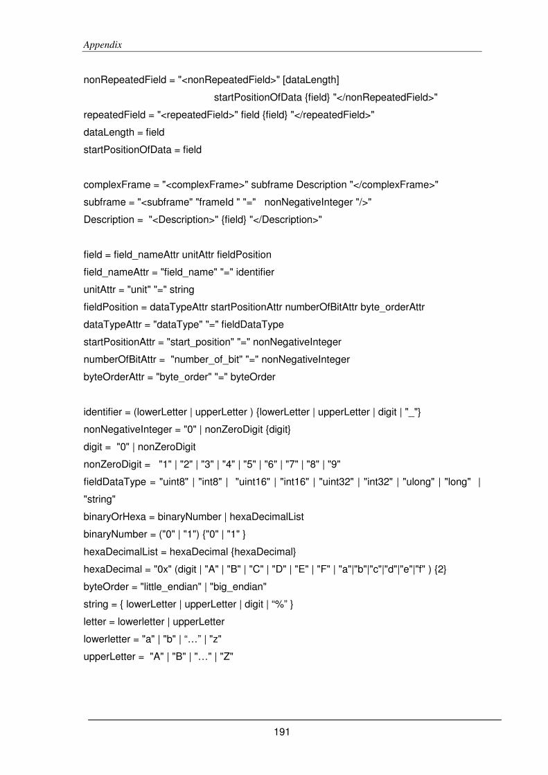
Appendix
191
nonRepeatedField = "<nonRepeatedField>" [dataLength]
startPositionOfData {field} "</nonRepeatedField>"
repeatedField = "<repeatedField>" field {field} "</repeatedField>"
dataLength = field
startPositionOfData = field
complexFrame = "<complexFrame>" subframe Description "</complexFrame>"
subframe = "<subframe" "frameId " "=" nonNegativeInteger "/>"
Description = "<Description>" {field} "</Description>"
field = field_nameAttr unitAttr fieldPosition
field_nameAttr = "field_name" "=" identifier
unitAttr = "unit" "=" string
fieldPosition = dataTypeAttr startPositionAttr numberOfBitAttr byte_orderAttr
dataTypeAttr = "dataType" "=" fieldDataType
startPositionAttr = "start_position" "=" nonNegativeInteger
numberOfBitAttr = "number_of_bit" "=" nonNegativeInteger
byteOrderAttr = "byte_order" "=" byteOrder
identifier = (lowerLetter | upperLetter ) {lowerLetter | upperLetter | digit | "_"}
nonNegativeInteger = "0" | nonZeroDigit {digit}
digit = "0" | nonZeroDigit
nonZeroDigit = "1" | "2" | "3" | "4" | "5" | "6" | "7" | "8" | "9"
fieldDataType = "uint8" | "int8" | "uint16" | "int16" | "uint32" | "int32" | "ulong" | "long" |
"string"
binaryOrHexa = binaryNumber | hexaDecimalList
binaryNumber = ("0" | "1") {"0" | "1" }
hexaDecimalList = hexaDecimal {hexaDecimal}
hexaDecimal = "0x" (digit | "A" | "B" | "C" | "D" | "E" | "F" | "a"|"b"|"c"|"d"|"e"|"f" ) {2}
byteOrder = "little_endian" | "big_endian"
string = { lowerLetter | upperLetter | digit | “%” }
letter = lowerletter | upperLetter
lowerletter = "a" | "b" | “…” | "z"
upperLetter = "A" | "B" | "…" | "Z"

Appendix
192
A.2 The syntax graphs of the STDL.
A.2.1 Frame Structure
A.2.2 Frame Attributes
A.2.3 Frame Description

Appendix
193
A.2.3.1 Frame Header Description
A.2.3.2 Frame Content Description

Appendix
194
A.2.4 Data Type
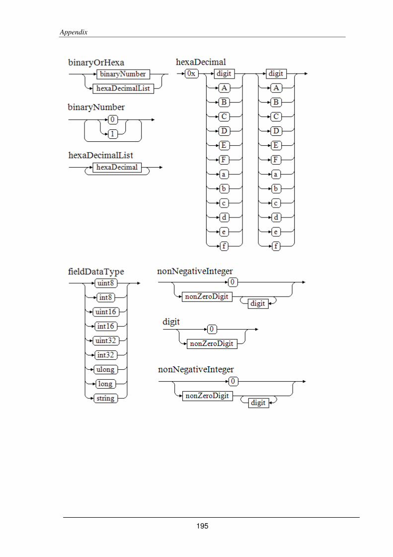
Appendix
195