a sufficient statistics approach for welfare analysis of
TRANSCRIPT

Kyoto University, Graduate School of Economics Discussion Paper Series
A Sufficient Statistics Approach for Welfare Analysis of Oligopolistic Third-Degree Price Discrimination
Takanori Adachi and Michal Fabinger
Discussion Paper No. E-21-005
Graduate School of Economics Kyoto University
Yoshida-Hommachi, Sakyo-ku Kyoto City, 606-8501, Japan
October 2021

A Sufficient Statistics Approach for Welfare Analysis of
Oligopolistic Third-Degree Price Discrimination∗
Takanori Adachi† Michal Fabinger‡
October 26, 2021
Abstract
This paper proposes a sufficient statistics approach to welfare analysis of third-degree
price discrimination in differentiated oligopoly. Specifically, our sufficient conditions for
price discrimination to increase or decrease aggregate output, social welfare, and con-
sumer surplus simply entail a cross-market comparison of multiplications of two or three
of the sufficient statistics—pass-through, conduct, and profit margin—that are functions
of first-order and second-order elasticities of the firm’s demand. Notably, these results
are derived under a general class of demand, and can be readily be extended to accom-
modate heterogeneous firms. These features suggest that our approach has potential for
conducting welfare analysis without a full specification of an oligopoly model.
Keywords: Third-Degree Price Discrimination; Oligopoly; Sufficient Statistics.
JEL classification: D43; L11; L13.
∗We are grateful to Inaki Aguirre, Jacob Burgdorf, Susumu Cato, Yong Chao, Jacob Gramlich, MakotoHanazono, Hiroaki Ino, Noritaka Kudoh, Toshifumi Kuroda, Jeanine Miklos-Thal, Ignacio Palacios-Huerta, DanSasaki, Susumu Sato, Nicolas Schutz, Shohei Tamura, Tsuyoshi Toshimitsu, Yusuke Zennyo, and conferenceand seminar participants at numerous places for helpful comments and discussions. An earlier version ofthe paper was circulated under the title of “Output and Welfare Implications of Oligopolistic Third-DegreePrice Discrimination.” Adachi acknowledges a Grant-in-Aid for Scientific Research (C) (15K03425, 18K01567,21K01440) from the Japan Society of the Promotion of Science. Fabinger acknowledges a Grant-in-Aid forYoung Scientists (A) (26705003) from the Society. All remaining errors are our own.†Graduate School of Management and Graduate School of Economics, Kyoto University, Japan. E-mail:
[email protected]‡Graduate School of Economics, University of Tokyo, Japan. E-mail: [email protected]

1 Introduction
This paper explores the welfare effects of third-degree price discrimination in oligopoly and
its output implications as well as the effects on consumer surplus. Specifically, we consider a
fairly general setting, and present the sufficient conditions under which oligopolistic third-degree
price discrimination increases or decreases aggregate output, consumer surplus, and Marshallian
social welfare (i.e., the sum of the consumer and producer surpluses) when all discriminatory
markets are served even in the absence of price discrimination. Our analysis is firstly developed
under firm symmetry, and is extended to accommodate heterogeneous firms. Moreover, our
analysis permits a moderate degree of cost differences to exist across separate markets. To
do all these tasks, we employ the sufficient statistics approach as a unifying methodology: a
technique often used in public economics (Chetty 2009; Kleven 2021) as well as macroeconomics
(Barnichon and Mesters 2021).
Under third-degree price discrimination, consumers are segmented into separate markets
and charged different unit prices in accordance with their identifiable characteristics (e.g., age,
occupation, location, or time of purchase). In contrast, all consumers are charged the same
price if third-degree price discrimination is not practiced (i.e., “uniform pricing”). Without loss
of generality, the case of two markets can be considered to understand how price discrimination
might change output and welfare in each market. The prevailing price is identical in both
markets if all firms are symmetric. In this situation, if a discriminatory price becomes greater
than the uniform price in one market, and the unit price decreases in the other market, Robinson
(1933) calls the former market a “strong” market (s), and the latter a “weak” market (w). More
formally, this situation is expressed by p∗s > p > p∗w, where p∗s and p∗w are the equilibrium prices
under price discrimination in the strong and the weak markets, respectively, and p is the uniform
price.1 Given such a price change, price discrimination increases output and social welfare in
the weak market, but decreases them in the strong market. What are the overall effects of the
price change?
In the analysis below, we follow Leontieff (1940), Silberberg (1970), Schmalensee (1981),
Holmes (1989), and Aguirre, Cowan, and Vickers (2010) to add the constraint ps − pw = t,
1In this paper, price discrimination is present when ps > pw, i.e., when prices between markets are notuniform. As Clerides (2004, p. 402) states, once cost differentials are allowed, “there is no single, widelyaccepted definition of price discrimination.” To understand this, consider symmetric firms and let mcs andmcw be the marginal cost at equilibrium output in markets s and w, respectively (they do not necessarily haveto be constants for any output levels). Then, two alternative definitions can be considered. One is the margindefinition: price discrimination occurs when ps−mcs > pw−mcw. The other one is the markup definition as perStigler (1987): price discrimination occurs when ps/mcs > pw/mcw. Our simpler definition is aligned with theformer definition, and employed for its tractability and connectivity to the existing literature on third-degreeprice discrimination with no cost differentials. Moreover, our definition of price discrimination coincides withwhat Chen and Schwartz (2015) and Chen, Li and Schwartz (2021) call “differential pricing.” As long as costdifferentials are sufficiently small, these differences will not significantly alter the results because if mcs = mcw,these three definitions are equivalent.
1

where t ≥ 0 is interpreted as an artificial constraint on the profit maximization problem for
oligopolistic firms under symmetry. Then, the regime change, which is discrete in its nature,
is now measured by t and is continuously connected between t = 0 as uniform pricing and
t∗ ≡ p∗s − p∗w as price discrimination in equilibrium. This formulation enables us to describe
social welfare as a function of t, W (t), and characterize W ′(t) in terms of economic concepts
based on elasticity terms of market demand. In this way, whether social welfare improves or
deteriorates by this global change of the regime can be determined. This methodology shares
the central idea of the sufficient statistics approach where the welfare consequences of policy
changes are derived “in terms of estimable elasticities” (Kleven 2021, p. 516) “rather deep
primitives” (Chetty 2009, p. 452). One benefit of focusing on sufficient statistics rather than
deep parameters in conducting welfare analysis is that one can focus on the deeper structure
that is “robust across a broad class of underlying models,” (Kleven 2021, p. 535) without a
specification of market demand. If we instead start with a particular class of demand, it
remains unclear to what extent the welfare analysis is valid under another class of market
demand.2
Our sufficient conditions for oligopolistic price discrimination to increase or decrease ag-
gregate output, social welfare, and consumer surplus are provided by means of a cross-market
comparison of the multiplications of two or three of the following economic concepts: (i) profit
margin, which is the difference between price and marginal cost (µ ≥ 0); (ii) pass-through, i.e.,
how the price responds to a small change in marginal cost (ρ > 0); and (iii) conduct, which
measures the degree of market monopolization (θ ∈ [0, 1]). These three sufficient statistics are
determined by the following two first-order and two second-order elasticities: (a) the own price
elasticity of the firm’s demand (εown), (b) the cross price elasticity of the firm’s demand (εcross),
(c) the curvature of the firm’s demand (αown), and (d) the elasticity of the cross-price effect of
the firm’s demand (αcross).
Specifically, in a series of propositions, we demonstrate that the product of conduct and
pass-through, θρ, is an important measurement for determining the output effects, whereas the
product of all three concepts, θµρ, provides the sufficient condition for the change in welfare.
Intuitively, the product of conduct and pass-through measures how output in each individual
market changes in response to a marginal change in price. To evaluate a marginal change
in welfare, profit margin should be considered because it measures the welfare gain or loss
2One may criticize that sufficient statistics are only endogenous variables by holding that a sufficient conditionis meaningful only when it consists of exogenous parameters. However, in equilibrium, our sufficient conditionsare functions of exogenous parameters for the same reason that in equilibrium, endogenous variables are functionsof exogenous variables, as demonstrated in Section 4. However, deep parameters themselves do not always alloweconomic interpretations in a direct manner; for example, in the case of linear demand, the slope coefficient is notdirectly to related to demand elasticity. In contrast, sufficient statistics such as elasticities almost always haveeconomic interpretations. This is the benefit from the sufficient statistics approach because welfare analysis canbe conducted based on economic concepts one-level higher that underlie a plausible class of model specification.
2

that results from a marginal change in quantity under imperfect competition in which the price
exceeds marginal cost. In this way, the welfare implications can be obtained by means of a cross-
market comparison of the quantity change multiplied by the profit margin. To determine the
effect on consumer surplus, the product of profit margin and pass-through, µρ, is important
because it measures the price change multiplied by the level of output. However, one may
wonder if this sufficient statistics approach is valid once firm symmetry is relaxed. Section 6
provides a positive answer: no additional complications are necessary to extend our analysis
under firm symmetry.
Existing literature on third-degree price discrimination has a centennial tradition, pioneered
by Pigou (1920) and Robinson (1933), with their main focus on whether price discrimination in-
creases or decreases social welfare (see Varian (1989); Armstrong (2006, 2008); and Stole (2007)
for comprehensive surveys of this literature). Among others, Schmalensee (1981) and Aguirre,
Cowan, and Vickers (hereafter, ACV) (2010) study how demand curvatures relate to output
and welfare effects. Third-degree price discrimination necessarily entails allocative inefficiency
because some consumers exist who have the same marginal utility but face different prices
simply because they belong to different markets. Thus, for third-degree price discrimination to
increase social welfare, it must sufficiently expand aggregate output to offset such misallocation
across markets. Schmalensee (1981) shows that an increase in aggregate output is a necessary
condition for third-degree price discrimination to increase social welfare—a conclusion that is
generalized by Varian (1985) and Schwartz (1990)—and ACV (2010) identify a sufficient con-
dition for price discrimination to raise social welfare: inverse demand in the weak market is
more convex than that in the strong market at the discriminatory prices. Figure 1 provides
a graphical illustration: if uniform pricing is implemented instead, welfare loss in the weak
market due to the output reduction that has arisen under price discrimination is sufficiently
large (Panel b) as compared to the welfare gain in the strong market (Panel a).
However, in this approach, a change in welfare is not predictable if the demand primitives
do not satisfy the conditions that are focused on. In addition, most of these studies analyze
monopolistic third-degree discrimination: to date, “there are virtually no predictions as to
how discrimination impacts welfare” (Hendel and Nevo 2013, p. 2723; emphasis added) when
oligopolistic competition is considered. For example, Holmes (1989) employs the same technique
used by Schmalensee (1981) and ACV (see Section 3 for details) to examine the output effects of
third-degree price discrimination in a symmetric oligopoly. However, Holmes (1989) provides no
welfare predictions (see also Dastidar 2006).3 In this paper, we contribute to the literature by
3In a similar vein, Armstrong and Vickers (2001) consider a model of symmetric duopoly with productdifferentiation a la Hotelling (1929), and study the consequences of third-degree price discrimination in thecompetitive limit around zero transportation costs wherein the equilibrium prices are almost equal to marginalcost. Under this setting, Armstrong and Vickers (2001) show that price discrimination decreases social welfareif the weak market has a lower value of price elasticity of demand (Adachi and Matsushima (2014) also derivea similar result by assuming linear demand in a standard model of symmetrically differentiated duopoly). Our
3

(a) Strong Market (b) Weak Market
Figure 1: Welfare Comparison in terms of Demand Curvatures (Aguirre, Cowan, and Vickers2010)
providing fairly general conditions regarding whether oligopolistic price discrimination increases
or decreases aggregate output, social welfare, and consumer surplus.
Our study is also in line with Mrazova and Neary (2017) who show the usefulness of the
demand manifold—the relationship between demand elasticity and convexity which is not as-
cribed to a function or a correspondence—in comparative statics by suggesting the linkage
between these first- and second-order elasticities and sufficient statistics such as markup and
pass-through as shown in an empirical study by De Loecker, Goldberg, Khandelwal, and Pavc-
nik (2016).4 Mrazova and Neary (2017) point out that one of the advantages of working with
the demand manifold instead of the demand function per se is that it is clearer to understand
results from comparative statics and counterfactual experiments because demand elasticity and
convexity are more closely related to them than demand primitives themselves are. However,
Mrazova and Neary (2017) mainly focus on perfect and monopolistic competition: when firm
heterogeneity is taken into account, only cost/productivity heterogeneity a la Melitz (2003) is
considered. In other words, neither εcross nor αcross appears in Mrazova and Neary’s (2017)
analysis because they do not consider product differentiation (firm heterogeneity on the de-
mand side). Therefore, they are able to focus on only two parameters, εown nor αown. While
we do not make use of their method, we explicitly consider imperfect competition based on
product differentiation, and further research would be promising to investigate how Mrazova
and Neary’s (2017) methodology is utilized for issued of imperfect competition such as this
paper aims to fill the gap between monopoly, such as in Schmalensee (1981) and ACV (2010), and Armstrongand Vickers’ (2001) competitive limit with respect to welfare implications. We thank Susumu Sato for suggestingthis interpretation.
4In our context, (i) profit margin is determined by the firm-level price elasticity (or the own price elasticity),(ii) pass-through is determined mainly by the demand curvature, and (iii) conduct is determined by the ratioof the industry-level elasticity to the firm-level elasticity. See the expressions (10) below for the case of pricediscrimination when market-wise elasticities are defined.
4

study.
The remainder of this paper is organized as follows. Section 2 presents our base model of
oligopolistic pricing with symmetric firms and constant marginal costs. Then, we derive the
sufficient statistics implications of aggregate output, social welfare, and consumer surplus in
Section 3. Subsequently, Section 4 provide parametric examples of three representative classes
of market demand differentiated goods that are often employed in applies studies are linear, CES
(constant elasticity of substitution), and logit to discuss how the sufficient statistics approach
works if demand primitives (expressed by parameters) demonstrate the results of the effects
on consumer surplus, and discuss the case of non-constant marginal costs. ... Section 5... In
Section 6, we argue that our differential method is readily extendible to the introduction of
firm heterogeneity. Finally, Section 7 concludes.5
2 The Model of Oligopolistic Pricing
For ease of exposition, we follow Holmes (1989) and ACV to consider the case of two symmetric
firms and two separate markets or consumer groups (hereafter, simply called “markets”): it
is straightforward to extend the following analysis to the case of more than two symmetric
firms and more than two separate markets.6 As explained in Introduction, we call one market
s (strong), where the equilibrium discriminatory price is higher than the equilibrium uniform
price, and the other w (weak), where the opposite is true. Two firms, A and B, have an identical
cost structure in each market. Specifically, each firm has an identical cost function, cm(qjm),
in market m = s, w, where qjm is firm j’s output (j = A, B). For simplicity of exposition, we
assume, with a bit abuse of notation, that firms have a constant marginal cost in each market
m, cm ≥ 0; here, cs and cw can be different. However, as mentioned again in Subsection 2.3
below, it is assumed that the strong market either has a higher marginal cost or only slightly
lower marginal cost so that its price still increases with price discrimination. In this sense, this
paper does not consider the role of cost differences in differential pricing (see Footnote 1 above).
2.1 Consumers
In market m = s, w, given firms A and B’s prices pAm and pBm, the representative consumer
purchases xAm > 0 and xBm > 0, and her (net) utility (i.e., surplus) is quasi-linear and thus
5In this paper, the only policy instrument is an enforcement of uniform pricing. Cowan (2018) studies amodel of monopoly to consider a more moderate instrument by which a government regulates the monopolist’sprofit margins or price-marginal cost ratios across different markets.
6We assume that resale between markets is impossible to prevent consumers in the strong market from beingbetter off buying the good at a lower price in the week market (see Boik (2017) for an empirical analysis ofoligopolistic third-degree price discrimination when arbitrage may matter).
5

written as
Um(xm)− pAmxAm − pBmxBm,
where xm = (xAm, xBm), and Um is three-times continuously differentiable, ∂Um∂xjm
> 0, ∂2Um∂x2jm
< 0,
j = A, B, and ∂2Um∂xAm∂xBm
< 0 (i.e., firms A and B produce substitutable products).
Inverse demands in market m, pjm = Pjm(xjm, x−j,m), are derived from the representative
consumer’s utility maximization (−j = A,B, −j 6= j ): ∂Um∂xjm
(xjm, x−j,m)− pjm = 0, which also
implicitly defines firm j’s direct demand in market m, xjm = xjm(pjm, p−j,m). We assume that
xjm(·) is twice continuously differentiable. Because of the assumptions regarding the utility,
firm j’s demand in market m decreases as its own price increases (∂xjm∂pjm
< 0), and it rises as the
rival’s price increases (∂xjm∂p−j,m
> 0; the firms’ products are substitutes).7 We also assume that
from a viewpoint of consumers, firms are symmetric: Um(x′, x′′) = Um(x′′, x′) for any x′ > 0 and
x′′ > 0. Then, the firms’ demands in market m are also symmetric: xAm(p′, p′′) = xBm(p′, p′′)
for any p′ > 0 and p′′ > 0. Because the firms’ technologies are also identical, we focus on
symmetric Nash equilibrium until we allow firm heterogeneity in Section 6.
We define the demand in symmetric pricing by qm(p) ≡ xAm(p, p). Another interpretation
of qm(p) is: both firms take 2qm(p) as the joint demand, “cooperatively” choose the same price
(behaving as an “industry”), and divide the joint demand equally to obtain qm(p). Note here
that
q′m(p) =∂xAm∂pA
(pA, p)
∣∣∣∣pA=p︸ ︷︷ ︸
<0 (ACV’s q′m)
+∂xAm∂pB
(p, pB)
∣∣∣∣pB=p︸ ︷︷ ︸
>0 (strategic)
. (1)
Thus, for q′m(p) to be negative, we assume that∣∣∣∂xAm∂pA
(p, p)∣∣∣ > ∂xAm
∂pB(p, p). Note also that by
symmetry, the following relationship also holds (this corresponds to Holmes’ (1989) Equation
4):∂xAm∂pA
(p, p)︸ ︷︷ ︸own
= q′m(p)︸ ︷︷ ︸industry
− ∂xBm∂pA
(p, p)︸ ︷︷ ︸strategic effects
.
This exchangeability is key in Holmes’ (1989) derivation below. Intuitively, each firm, under
symmetry,treats the industry demand qm(p) as if it is its own demand. Thus, how a firm’s
pricing behavior affects its own demand as an industry demand has the following two effects: a
small decrease in pA by firm A by deviating from the “coordinated” price p (i) not only raises
its own demand by ∂xAm∂pA
as the residual monopolist (taking the rival’s pricing as fixed; intrinsic
effects), (ii) firm A can now also obtain some of the consumers originally attached to firm B,
and this amount is ∂xBm∂pA
(strategic effects).
7Here,∂2xjm∂p2j
(p, p) can be positive, zero or negative. Following Dastidar’s (2006, p. 234) Assumption 2 (iv),
we assume that∂2xjm∂p2j
(p, p) +∂2xjm∂pj∂p−j
(p, p) ≤ 0.
6

Under symmetric pricing, we are able to define, following Holmes (1989, p. 245), the price
elasticity of the industry’s demand by
εIm(p) ≡ −pq′m(p)
qm(p).
This corresponds to η in ACV (p. 1603) as well as εD in Weyl and Fabinger (2013, p. 542): it
should not “be confused with the elasticity of the residual demand that any of the firms faces.”
Similarly, the own and the cross price elasticities of the firm’s demand are defined by
εownm (p) ≡ − p
qm(p)
∂xAm∂pA
(p, p) > 0
and by
εcrossm (p) ≡ p
qm(p)
∂xBm∂pA
(p, p) > 0,
respectively. Then, Holmes (1989) shows that under symmetric pricing, εownm (p) = εIm(p) +
εcrossm (p) holds.8 This implies that the own-price elasticity must be equal to or greater than
the industry’s elasticity and greater than the cross-price elasticity (i.e., εownm (p) ≥ εIm(p) and
εownm (p) > εcrossm (p)).
2.2 Firms
Firm j’s profit in market m is written as
πjm(pm) = (pjm − cm)xjm(pm), (2)
where pm = (pjm, p−j,m). As in Dastidar’s (2006, pp. 235-6) Assumptions 3 and 4, for the
existence and the global uniqueness of pricing equilibrium under either uniform pricing or
price discrimination, we assume that for each firm j = A,B,∂2πjm∂p2jm
< 0,∂2πjm
∂pjm∂p−j,m> 0, and
−∂2πjm/(∂pjm∂p−j,m)
∂2πjm/∂p2jm< 1 (see Dastidar’s (2006) Lemmas 1 and 2 for the existence and the unique-
ness). We then define the first-order partial derivative of the profit in market m, evaluated at
a symmetric price p, by
∂pπm(p) ≡ ∂πjm(pjm, p−j,m)
∂pjm
∣∣∣∣pjm=p−j,m=p
= qm(p) + (p− cm)∂xAm∂pA
(p, p). (3)
8In general, when there are N ≥ 2 firms, this identity still holds if the cross price elasticity is defined byεcrossm (p) ≡ (N − 1) p
qm(p)∂xBm∂pA
(p, p).
7
Then, under symmetric discriminatory pricing, p∗m satisfies ∂pπm(p∗m) = 0 for m = s, w. Under
symmetric uniform pricing, p is a (unique) solution of ∂pπs(p) + ∂pπw(p) = 0. Throughout
this paper, we consider the situation where the weak market is open under uniform pricing (for
which qw(p∗s) > 0 is a sufficient condition).9
2.3 Equilibrium
The equilibrium discriminatory price in market m = s, w, p∗m, satisfies the following Lerner
formula:
εownm (p∗m)p∗m − cmp∗m
= 1.
This shows that the discriminatory price in market m approaches to the marginal cost as the
own-price elasticity for the firm, εownm (p∗m), becomes large. Because of Holmes’ (1989) elasticity
formula explained above, εownm (p∗m) can be large (i) when εIm(p∗m) is very large even if εcrossm (p∗m)
is close to zero, or (ii) when εcrossm (p∗m) is very large even if εIm(p∗m) is close to zero. Evidently,
if there are no cost differentials between markets, which market is strong or weak is solely
determined by the difference in the own-price elasticity. As mentioned above, we assume that
the marginal cost in the strong market is not sufficiently low to assure that p∗s > p > p∗w indeed
holds.10,11
Lastly, let ym be per-firm (symmetric) market share of output in market m, that is,
ym(ps, pw) ≡ qm(pm)qs(ps)+qw(pw)
. Then, the equilibrium uniform price, p ≡ p(cs, cw), satisfies:
∑m=s,w
ymεownm (p)
p− cmp
= 1,
where ym ≡ ym(p(cs, cw), p(cs, cw)) for m = s, w.12 In this way, the equilibrium level of uniform
9Note that qw(p) > qw(p∗s) because qw(·) is strictly decreasing and p∗s > p. Thus, if qw(p∗s) > 0, then theweak market is open under uniform pricing, i.e., qw(p) > 0. Alternatively, we would be able to show that thereexist cs and cs, cs < cs, such that p∗s > p∗w and qw(p) > 0 for cs ∈ (cs, cs) in a similar spirit of Adachi andMatsushima (2014).
10See Nahata, Ostaszewski, and Sahoo (1990) for an example of all discriminatory prices being lower thanthe uniform price with a plausible demand structure under monopoly. In the case of oligopoly, Corts (1998)show that best-response asymmetry, in which firms differ in ranking strong and weak markets, is necessary forall discriminatory prices to be lower than the uniform price (“all-out price competition”). As long as symmetricfirms are considered, this case never arises.
11When price discrimination is allowed, each firm may not price discriminate even if it is allowed to doso because it is still able to set a uniform price (i.e., it is not forced to price discriminate). We assume thatπjm(·, p∗−j,m) is strictly increasing (decreasing) at pjm = p in market m = s (m) and thus firm j has an incentiveto deviate from the equilibrium uniform price if the other firm chooses p∗−j,s and p∗−j,w, and that πjm(·, p∗−j,m)attains the global optimum at pjm = p∗jm.
12If there are no cost differentials, i.e., cs = cw (≡ c), then the formula is simpler:
p− cp
=1∑
m=s,w ymεownm (p)
8

price is determined by the market-share weighted average of the own price elasticities, whereas
the equilibrium level of discriminatory price solely depends on the firm’s own price elasticity in
that market. In the rest of the paper, the dependence of the equilibrium price is often implicit
when there are no confusions. In particular, the superscript star (the upper bar) denotes price
discrimination (uniform pricing). For example, we write (εIm)∗ ≡ εIm(p∗m) and εIm ≡ εIm(p) as
the industry’s elasticities in equilibrium.
3 Welfare Effects
As mentioned in Introduction, we add the constraint ps − pw = t, where t ≥ 0, to the firms’
profit maximization problem.13 Then, we express social welfare (as well as aggregate output
and consumer surplus) as a function of t in [0, t∗], where t = 0 corresponds to uniform pricing,
and t = t∗ ≡ p∗s−p∗w to price discrimination. Note that under this constrained problem of profit
maximization, pw satisfies ∂pπs(pw + t) + ∂pπw(pw) = 0. Thus, we write the solution by pw(t).
Then, we define ps(t) ≡ pw(t) + t. Applying the implicit function theorem to this equation
yields to p′w(t) = − π′′sπ′′s+π′′w
< 0 and p′s(t) = π′′wπ′′s+π′′w
> 0, where
π′′m(p) ≡ q′m(p) +∂xAm∂pA
(p, p) + (p− cm)d
dp
(∂xAm∂pA
(p, p)
)= ∂2
pπm(p)︸ ︷︷ ︸ACV’s π′′m
+∂xAm∂pB
(p, p) + (p− cm)∂2xAm∂pB∂pA
(p, p)︸ ︷︷ ︸strategic
, (4)
and ∂2pπm(p) is defined by
∂2pπm(p) ≡
[2 + (p− cm)
∂2xAm(p, p)/∂p2A
∂xAm(p, p)/∂pA
]∂xAm∂pA
(p, p). (5)
The latter corresponds to ACV’s (p. 1603) π′′m(p), and the second and third term arise due to
oligopoly. Here, in each m, π′′m(p) is assumed to be negative for all p ≥ 0.14
We define the representative consumer’s utility in symmetric pricing by Um(q) = Um(q, q).
as shown by Holmes (1989, p. 247): the markup rate (common to all markets) is equal to the inverse of theaverage of own-price elasticities weighted by the output shares.
13Alternatively, Vickers (2020) analyzes properties of social welfare and consumer surplus as a scalar argumentto make a comparison between price discrimination and uniform pricing in monopoly. Vickers (2020) especiallyfocuses on the case where quantity elasticity or inverse demand curvature is constant for all markets. See alsoCowan (2017) for an analysis of the role of price elasticity and demand curvature in determining the effects ofmonopolistic third-degree price discrimination.
14ACV’s Appendix A discusses the concavity of the profit function.
9

Then, social welfare under symmetric pricing as a function of t is written as
W (t) ≡ Us(qs[ps(t)]) + Uw(qw[pw(t)])− 2cs · qs[ps(t)]− 2cw · qw[pw(t)]
= (U ′s − 2cs) · q′s · p′s(t) + (U ′w − 2cw) · q′w · p′w(t),
which impliesW ′(t)
2= [ps(t)− cs] · q′s · p′s(t) + [pw(t)− cw] · q′w · p′w(t) (6)
because U ′m = ∂Um∂qA
+ ∂Um∂qB
= 2∂Um∂qA
(by symmetry). On the other hand, aggregate output under
symmetric pricing is given by
Q(t) = Qs(t) +Qw(t) = 2 {qs[ps(t)] + qw[pw(t)]} ,
whereas consumer surplus is defined by replacing cm in W (t) by pm(t) to define
CS(t) = Us(qs[ps(t)]) + Uw(qw[pw(t)])− 2ps(t) · qs[ps(t)]− 2pw(t) · qw[pw(t)].
As argued above, W (t), Q(t), and CS(t) are all functions of t ∈ [0, t∗]. The regime change
from uniform pricing to price discrimination is captured by a parameter shift from t = 0 to
t = t∗, and vice versa. However, if these functions are globally concave in this range, then the
local sign at t = 0 or t∗ may predict the sign from the regime change. Specifically, consider a
representative function, F (t). If the global concavity of F (t) is assured, then F (t) behaves in
either manner:
1. If F ′(0) ≤ 0, then F (t)2
is monotonically decreasing in t, and as a result ∆F2
= F (t∗)−F (0)2
< 0;
price discrimination decreases F .
2. If F ′(0) > 0, then F (t)2
either
(a) is monotonically increasing (if F ′(t∗) > 0, this is true), and as a result, ∆F2> 0;
price discrimination increases F .
(b) first increases, and then after the reaching the maximum (where F ′(t) = 0), decreases
until t = t∗. In this case, price discrimination may increase or decrease F : it
cannot be determined whether ∆F2< 0 or ∆F
2> 0 without further functional and/or
parametric restrictions.
3.1 Curvatures, Conduct, and Pass-Through
In this subsection, we first introduce second-order elastiticities–demand curvatures–to argue
how π′′m is expressed in terms of the first- and second-order elasticities. We then define two of
10

the three sufficient statistics that play an important role in determining the output and welfare
effects of third-degree price discrimination in oligopoly in Subsections 5.1, 3.2, and 5.2.
3.1.1 Curvatures
To proceed further, we define the curvature of the firm’s (direct) demand in market m by
αownm (p) ≡ − p
∂xAm(p, p)/∂pA
∂2xAm∂p2
A
(p, p),
which measures the convexity/concavity of the firm’s direct demand, and corresponds to αm(p)
in Aguirre, Cowan and Vickers 2010, p. 1603). The elasticity of the cross-price effect of the
firm’s direct demand in market m is defined by
αcrossm (p) ≡ − p
∂xAm(p, p)/∂pA
∂2xAm∂pB∂pA
(p, p),
which does not appear in monopoly. Here, αownm and αcrossm are positive (resp. negative) if and
only if ∂2xAm∂p2A
and ∂2xAm∂pB∂pA
are positive (resp. negative), respectively. Note also that the sign of
αownm indicates whether the firm’s own part of the demand slope under symmetric pricing given
the rival’s price p, ∂xAm∂pA
(·, p), is convex (αownm is positive) or concave (αownm is negative). On the
other hand, αcrossm measures to what extent the rival’s price level matters to how many of the
firm’s customers switch to the rival’s product when the firm raises its own price (∂xAm∂pA
). Thus,
a large αcrossm implies that ∂xAm∂pA
is very responsive to a change in pB, and vice versa.
Note here that Equation (5) implies that
∂2pπm(p) = −{2− p− cm
p︸ ︷︷ ︸=Lm(p)
[− p∂xAm∂pA
(p, p)
∂2xAm∂p2
A
(p, p)︸ ︷︷ ︸=αownm (p)
]}[− p
qm(p)
∂xAm∂pA
(p, p)︸ ︷︷ ︸=εownm (p)
]qm(p)
p
= −[2− Lm(p)αownm (p)]εownm (p)qm(p)
p,
where
Lm(p) ≡ p− cmp
is the markup rate (i.e., the Lerner index). Therefore, from Equation (4), π′′m(p) is expressed
in terms of the four elasticities (εownm , εcrossm , αownm , and αcrossm ) as well as qm(p) and p itself:
π′′m(p) = −[2− Lm(p)αownm (p)]εownm (p)qm(p)
p+ [
p
qm(p)
∂xAm∂pB
(p, p)︸ ︷︷ ︸=εcrossm (p)
]qm(p)
p
11

−p− cmp︸ ︷︷ ︸
=Lm(p)
[− p∂xAm∂pA
(p, p)
∂2xAm∂pB∂pA
(p, p)︸ ︷︷ ︸=αcrossm (p)
][p
qm(p)
∂xAm∂pA
(p, p)︸ ︷︷ ︸=−εownm (p)
]qm(p)
p
= −{[2− Lm(αownm + αcrossm )]εownm − εcrossm }qmp. (7)
3.1.2 Conduct
Next, we define the conduct parameter 15 in market m by θm(p) ≡ 1 − ADRm(p), where
ADRm(p) is the aggregate diversion ratio (Shapiro 1996) in market m, defined by
ADRm(p) ≡ −∂xBm(p, p)/∂pA∂xAm(p, p)/∂pA
=εcrossm (p)
εownm (p).
Here, ADRm(p) measures the intensity of rivalness : if ADRm(p) is close to one, consumers who
leave a firm as a response to an increase in its price are mostly switching to its rival’s product.
In this way, ACV’s derivation for the case of monopoly, where Schmalensee’s (1981) method is
utilized, is connected to Weyl and Fabinger’s (2013) condition in the case of symmetric oligopoly.
In particular, ACV’s (p. 1606) Proposition 2 (a sufficient condition for price discrimination to
increase social welfare) is extended to the case of oligopoly in a simpler manner, using the
concept of pass-through introduced later in this subsection.16
As Weyl and Fabinger (2013, p. 544) argue, θm(p) captures the degree of industry-level
brand loyalty or stickiness17 in market m. To see this, note that the conduct parameter is also
15This term originates from the empirical literature where conduct itself is a target of estimation (“parameter”)without an exact specification of strategic interaction (see, e.g., Bresnahan 1989; Genesove and Mullin 1998;and Corts 1999).
16Alternatively, Weyl and Fabinger (2013, p. 531) and Adachi and Fabinger (2021) define the conduct param-eter in a market (which, in our interest in price discrimination, can be indexed by m) by θm ≡ LmεIm (their mcand εD are replaced by our cm and εIm, respectively) as the Lerner index adjusted by the elasticity of the indus-try’s demand. If the first-order condition is given for each market (that is, if full price discrimination is allowed),then θm(p) defined as in Weyl and Fabinger (2013) coincides with 1− ADRm(p) because pm−cm
pmεownm = 1 and
thus
Lm(p)εIm(p) =1
εFm(p)
(− p
qm(p)
)q′m(p)
= −qm(p)
p
1
∂xAm(p, p)/∂pA
(− p
qm(p)
)(∂xAm∂pA
(p, p) +∂xAm∂pB
(p, p)
)=
∂xAm(p, p)/∂pA + ∂xBm(p, p)/∂pA∂xAm(p, p)/∂pA
(by symmetry)
= 1−ADRm(p) ≡ θm(p)
is established. It turns out that this alternative definition is more tractable when firm heterogeneity is introducedin Section 6.
17Even if firms’ products have the same characteristics across different markets (with no product differentia-tion), brand loyalty may differ across markets, reflecting the differences in market characteristics (as summarizedin demand functions).
12

expressed by
θm(p) =εIm(p)
εownm (p),
where εownm (p) ≥ εIm(p). If εownm (p)→∞ as in the case of the price-taking assumption, θm(p) is
zero. On the other hand, if εownm (p) is equal to εIm(p), that is, the own elasticity is nothing but
the industry’s elasticity, then it is monopoly and θm(p) = 1.18
Note that the markup rate alone is not appropriate to measure the rivalness within market
m because it can be the case that pm is close to cm (the markup rate is close to zero) simply
because the price elasticity of the industry’s demand εIm(pm) is very large, whereas the brand
rivalness is so weak that the cross-price elasticity, εcrossm , remains very small (as a result, in
total, εownm is very large, which is actually the reason for the low markup rate). However, if
εcrossm is close to εownm (i.e., almost of all consumers who leave a firm as a response to its price
increase are switching to other rivals’ products), then θm becomes close to zero irrespective of
the value of the markup rate. Thus, θm(p), which ranges between 0 and 1, better captures the
brand stickiness than Lm(p) does.
3.1.3 Pass-Through
Lastly, we define pass-through in market m by ρm ≡ ∂pm∂cm
. It is a function of t ∈ [0, t∗] when the
constrained problem is considered. In particular,
ρm[pm(t)] =
∂xAm/∂pAπ′′s + π′′w
for t < t∗
∂xAm/∂pAπ′′m
(≡ ρ∗m) for t = t∗
is obtained by applying the implicit function theorem to ∂pπs(pw + t) + ∂pπw(pw) = 0 for t < t∗
and ∂pπm(pm) = 0 for t = t∗ (i.e., under price discrimination).
If the marginal costs are constant, quantity pass-through in market m under price discrimina-
tion, which is defined by dq∗mdq
, where q is an exogenous amount of output with πjm(pjm, p−j,m) =
(pjm − cm)[xjm(pjm, p−j,m)− q], is expressed by
dq∗mdq
= q′m(p∗m) · dp∗m
dq=
q′m∂xAm∂pA
· ∂xAm∂pA
· dp∗m
dq=
(q′m∂xAm∂pA
)·
(∂xAm∂pA
π′′m
)= θ∗m · ρ∗m
because the first-order condition with q indicates dp∗mdq
= 1π′′m
.19
18Because pm−cmpm
εownm = 1 and εownm = εIm + εcrossm , it is verified that θm + pm−cmpm
εcrossm = 1. Thus, as long as
the products are substitutes (εcrossm > 0), θm is less than one.19Note that this is the case where
dq∗mdq is evaluated at q = 0: Miklos-Thal and Shaffer (2021a) derive a general
13

Equation (7) indicates that
ρ∗m =
∂xAm∂pA{
2− (Lm)∗[(αownm )∗ + (αcrossm )∗]− (εcrossm )∗
(εownm )∗
}∂xAm∂pA
=1
2− (εcrossm )∗+(αownm )∗+(αcrossm )∗
(εownm )∗
because (Lm)∗ = 1/(εownm )∗. Note here that in the case of monopoly ((εcrossm )∗ = 0 and (αcrossm )∗ =
0),
ρ∗m =1
2− (αownm )∗
(εownm )∗
(8)
and (αownm )∗
(εownm )∗corresponds to ACV’s (p. 1603) curvature of the inverse demand, σ∗m.
3.2 Social Welfare
First, Equation (6) implies that
W ′(t)
2= [ps(t)− p+ p− cs]q′s[ps(t)]p′s(t)
+[pw(t)− p+ p− cw]q′w[pw(t)]p′w(t)
= [ps(t)− p]q′s[ps(t)]p′s(t)︸ ︷︷ ︸<0
+ [pw(t)− p]q′w[pw(t)]p′w(t)︸ ︷︷ ︸<0
+∑m=s,w
(p− cm) q′m[pm(t)]p′m(t).
This derivation coincides with the case of monopoly as shown in ACV’s (p. 1604) Equality (3) if
there are no cost differentials (i.e., cs = cw ≡ c), with two minor modifications: (i) the left hand
side is W ′(t)2
rather than W ′(t) itself, and (ii) the last term of ACV’s Equality (3) is replaced
by Q′(t)2
rather than Q′(t) because (12)∑
m=s,w (p− cm) q′m[pm(t)]p′m(t) = (p− c) (Q′(t)2
). If cost
differentials are permitted, it is observed that an increase in the weighted aggregate output,∑m=s,w (p− cm) q′m[pm(t)]p′m(t) > 0, is necessary for price discrimination to increase social
welfare, as in the case of monopoly (see Part A of the Online Appendix for the case of a general
number of markets).
Now, we examine the effects of allowing third-degree price discrimination on social welfare
formula for q > 0, correcting Weyl and Fabinger’s (2013) arguments. If marginal costs are non-constant (seePart B of the Online Appendix ), then πjm(pjm, p−j,m) = pjm · [xjm(pjm, p−j,m)− q]− cm[xjm(pjm, p−j,m)− q]should be considered, where cm(·) is the cost function, and thus θ∗mρ
∗m is no longer the quantity pass-through
under price discrimination (that is, when q = 0). See Weyl and Fabinger (2013, p. 572) for a precise expressionof quantity pass-through with non-constant marginal costs.
14

in detail. Note first that
W ′(t)
2=
(− π′′sπ
′′w
π′′s + π′′w
)︸ ︷︷ ︸
>0
×(
(pw(t)− cw)q′w[pw(t)]
π′′w− (ps(t)− cs)q′s[ps(t)]
π′′s
). (9)
We then define the profit margin in market m by
µm(p) ≡ p− cm,
and follow ACV (p. 1605), who define
zm(p) ≡ µm(p)q′m(p)
π′′m(p),
which is “the ratio of the marginal effect of a price increase on social welfare to the second
derivative of the profit function.”20 However, our q′m and π′′m have strategic effects as Equations
(1) and (4) show.
As in ACV (p. 1605), we can write
W ′(t)
2=
(− π′′sπ
′′w
π′′s + π′′w
)︸ ︷︷ ︸
>0
{zw[pw(t)]− zs[ps(t)]} ,
and their lemma also holds in our case of oligopoly if we assume zm is increasing (the increasing
ratio condition for social welfare; IRCW).21 Then, the global concavity of W (t) is attained as
in the case of Q(t).
Now, using conduct, profit margin, and pass-through, we obtain the following sufficient
conditions for price discrimination to increase or decrease social welfare.
20Here, µm(p)q′m(p) can be interpreted as the marginal effect of a price increase on social welfare in marketm because:
d[
per-firm (normalized)︷ ︸︸ ︷1
2Um[qm(p)]− cmqm(p)]
dp= µm(p)q′m(p).
21Note that
z′m(p) =[µm(p)q′′m(p) + q′m(p)]π′′m(p)− µm(p)q′m(p)π′′′m(p)
[π′′m(p)]2
and thus, the IRCW is equivalent to
[µm(p)q′′m(p) + q′m(p)]π′′m(p) > µm(p)q′m(p)π′′′m(p).
Appendix B of ACV discusses sufficient conditions for the IRCW to hold in the case of monopoly.
15

(a) Strong Market (b) Weak Market
Figure 2: Welfare Comparison in terms of Sufficient Statistics
Proposition 1. Given the IRCW, if µ∗wθ∗wρ∗w > µ∗sθ
∗sρ∗s holds, then price discrimination in-
creases social welfare. Conversely, if
µwθwρwµsθsρs
≤ π′′w(p)
π′′s(p)
holds, then price discrimination decreases social welfare.
Proof. See Appendix, Part A.
Roughly speaking, if either (i) conduct (θ), (ii) profit margin (µ), or (iii) pass-through (ρ)
is sufficiently small in the strong market, then social welfare is likely to be higher under price
discrimination. In particular, if these three measures are calculated (or estimated) in each
separate market, then it would assist one to judge whether price discrimination is desirable
from a society’s viewpoint. As explained above, if the marginal costs are constant, θ∗mρ∗m is
interpreted as quantity pass-through: µ∗m × θ∗mρ∗m approximates the trapezoid generated by a
small deviation from (perfect) price discrimination that captures the marginal welfare gain in
the strong market and the marginal welfare loss in the weak market (see Figure 2). If the latter
is larger than the former, such a deviation lowers social welfare, and owing to the IRCW, this
argument extends globally so that the regime switch to uniform pricing definitely decreases
social welfare. Note that this comparison will be a little bit more involved when starting at
uniform pricing for the same reason as explained after Proposition 3.
This proposition also has the following attractive feature. Suppose that price discrimination
is being conducted. Then, to evaluate it from a viewpoint of social welfare, one only needs the
local information: first, θ∗m, µ∗m and ρ∗m for each m = s, w, are computed, and if the sufficient
16

condition above is satisfied, then the ongoing price discrimination is justified. In addition, to
compute θ∗m, µ∗m and ρ∗m in equilibrium, information on marginal cost is unnecessary : once a
specific form of demand function, qjm = xjm(pjm, p−j,m), is provided (and if the IRC is satisfied),
then the three variables are computed in the following manner:22
θ∗m = 1− (εcrossm )∗
(εownm )∗
ρ∗m =1
2− (εcrossm )∗+(αownm )∗+(αcrossm )∗
(εownm )∗
µ∗m =p∗m
(εownm )∗.
(10)
Thus, if the firm’s demand for each market m is estimated and the discriminatory price p∗m
is observed, then one can easily compute θ∗m, µ∗m, and ρ∗m, using up to second-order demand
characteristics.23
Why is the adjustment term,
π′′m(p) = −{[2− Lm(αownm + αcrossm )]εownm − εcrossm }qm(p)
p,
necessary for the deviation from uniform pricing? As stated above, θ∗mρ∗m is interpreted as
quantity pass-through under price discrimination in market m if marginal cost is constant.
Thus, the first part of the proposition simply claims that aggregate output is raised by price
discrimination if the marginal reduction in quantity caused by a small deviation from price
discrimination in the market where price discrimination increases output (i.e., the weak market)
is larger than the marginal increase in quantity in the strong market. The second part describes
the opposite case, although it does not permit a direct comparison because pass-through is not
defined market-wise unless the pricing regime is “perfect” or “full” price discrimination (i.e.,
t = t∗), where the first-order conditions are given market-wise. Note that if |π′′m| is small, then
πm is “flat,” and thus the price shift |∆pm| in response to some change would be large. Hence,
the role of π′′wπ′′s
is to adjust measurement units for ρwρs
. For example, if |π′′w| is very small, then
ρw is “over represented,” and thus it should be “penalized” so that the right hand side of the
inequality in the proposition becomes small. The same argument also applies to the analysis
of social welfare and consumer surplus below.
Even if there are no cost differentials (i.e., cs = cw), this expression cannot be further
simplified. In other words, this expression is already robust to the inclusion of cost differentials.
Now, if we further assume that there are no strategic effects (i.e., θm = 1), then the condition
22An alternative expression for µ∗m is µ∗m = cm(εownm )∗−1 if the cost information is used.
23It should be emphasized that the second-order supply property, i.e., the derivative of marginal cost, wouldbe necessary if non-constant marginal cost is allowed, as suggested by Adachi and Fabinger (2021) in the contextof general “taxation” (pure taxation and other additional costs from external changes).
17

µ∗wθ∗wρ∗w ≥ µ∗sθ
∗sρ∗s becomes p∗s−c
p∗w−c≤ 1/ρ∗s
1/ρ∗w, which coincides with
p∗w − c2− σ∗w
≥ p∗s − c2− σ∗s
in Proposition 2 of ACV (p. 1606), where σ∗m is what they call the curvature of the inverse
demand function (under price discrimination), because of σ∗m = (αownm )∗
(εownm )∗(see the last part of
Subsubsection 3.1.3 above) and Equation (8). Thus, price discrimination increases social welfare
“if the discriminatory prices are not far apart and the inverse demand function in the weak
market is locally more convex than that in the strong market” (ACV, p. 1602). As compared
to Figure 1, Figure 2 shows the usefulness of the sufficient statistics in welfare evaluation.
4 Parametric Examples of Market Demand
To consider the following parametric examples of market demand, we assume that there are
two markets (strong and weak), and two symmetric firms. These demand functions are among
the commonly-used demand systems (Quint 2014). Note that to save notation, the same βm
is repeatedly used in the following three examples, but with different meanings (similarly, ωm
appears twice in the first and the third examples).
Recall that Proposition 1 provides a sufficient condition for price discrimination to increase
social welfare. By noting that
sign[W ′(0)] = sign[µw(p)q′w(p)
π′′w(p)− µs(p)
q′s(p)
π′′s(p)]
from Equation (6), we are also able to provide another sufficient condition for price discrimi-
nation to decrease social welfare.
Proposition 2. Given the IRCW, if the profit margin in strong market relative to the weak
market at the uniform price p is sufficiently large, i.e.,
µsq′sπ′′s≥ µw
q′wπ′′w
, (11)
then price discrimination decreases social welfare.
If there are no strategic effects (i.e., ∂xBm/∂pA = 0 or θm(p) = 1), then π′′m(p)q′m(p)
= 2 −Lm(p)αownm , and Inequality (11) above reduces to µs
µw≥ 2−Ls(p)αowns
2−Lw(p)αownw. On the other hand, if there
are no cost differentials (i.e., cs = cw ≡ c), then Inequality (11) above reduces to π′′w(p)q′w(p)
≥ π′′s (p)q′s(p)
because the profit margins are the same in the two markets. Thus, if there are no strategic
effects and no cost differentials, then inequality (11) coincides with ACV’s (p. 1605) Proposition
1 (αowns ≥ αownw in our notation; in their notation, αs(p) ≥ αw(p)) because Ls(p) = Lw(p). That
18

Linear CES Logit
Conduct θ∗m 1− δm2(1− βm)
2− βm − βmηm1− 2q∗m1− q∗m
Profit margin µ∗m(1− δm)(ωm − cm)
2− δm2(1− βm)(1− βmηm)
βm[1 + (1− 2βm)ηm]cm
1
βm(1− q∗m)
Pass-through ρ∗m1
2− δm2− βm − βmηm
βm[1 + (1− 2βm)ηm]
1
1− q∗m(1−2q∗m)(1−q∗m)2
Elasticities
First-order (own) εownm
(1− δm)ωm + cm(1− δm)(ωm − cm)
2− βm − βmηm2(1− βm)(1− βmηm)
βmpm(1− qm)
(cross) εcrossm
[(1− δm)ωm + cm]δm(1− δm)(ωm − cm)
βm(1− ηm)
2(1− βm)(1− βmηm)βmpmqm
Second-order (own) αownm 0(2− βmηm)(4− βm − 3βmηm)
2(1− βmηm)(2− βm − βmηm)βmpm(1− 2qm)
(Curvatures)
(cross) αcrossm 0 − βm(1− ηm)(2− βmηm)
2(1− βmηm)(2− βm − βmηm)
βmpmqm(1− 2qm)
1− qm
Table 1: Sufficient statistics under price discrimination (for duopoly). See below for the nota-tions.
is, the firm’s “direct demand function in the strong market is at least as convex as that in the
weak market at the nondiscriminatory price” (ACV, p. 1602).
Let the set of related parameters be denoted by Θ. If
G(Θ) ≡ µsµw− π′′s/q
′s
π′′w/q′w
and
H(Θ) ≡ µ∗sµ∗w− 1/(θ∗sρ
∗s)
1/(θ∗wρ∗w)
are defined, then G(Θ) ≥ 0 implies ∆W < 0 and H(Θ) < 0 implies ∆W > 0. Table 1 shows the
sufficient statistics as well as the first- and second-order elasticities under price discrimination
for the case of two symmetric firms (see Part C of the Online Appendix for details).
19

4.1 Linear Demand
Linear demand is derived from the quadratic utility of the representative consumer in market
m under symmetric product differentiation:
Um(xm) = ωm · (xAm + xBm)− 1
2
(βm [xAm]2 + 2γmxAmxBm + βm [xBm]2
),
which yields linear inverse demand, Pjm(xjm, x−j,m) = ωm − βmxjm − γmx−j,m, and the corre-
sponding direct demand in market m is
xjm(pjm, p−j,m;ωm, βm, γm) =1
(1− δ2m)βm
[ωm(1− δm)− pjm + δmp−j,m]
for firm j, where δm ≡ γmβm∈ [0, 1) is the strength of substitutability : if δm is close to one, market
m is approximated by perfect competition, whereas if δm is equal to zero, each firm behaves as
a monopolist.24
Now, consider
G(c, δ,β,ω) =p− csp− cw
− (2− δs)(1− δw)
(1− δs)(2− δw)≥ 0
as well as
H(c, δ,β,ω) =(ωs − cs)(1− δs)(2− δw)
(ωw − cw)(1− δw)(2− δs)− (2− δs)(1− δw)
(1− δs)(2− δw)< 0.
If there is no product differentiation (i.e., monopoly: γm = 0 and hence δm = 0), then
G(c, δ,β,ω) =p− csp− cw
− 1
so that G(c, δ,β,ω) ≥ 0⇔ cw ≥ cs. Similarly,
H(c, δ,β,ω) =p∗s − csp∗w − cw
− 1
24Note that the demand system here can be interpreted as the Levitan-Shubik demand system (Shubik andLevitan 1980), in which the representative consumer’s utility in our two-firm case is given by
Um(xm) = ωm · (xAm + xBm)− 1
2λm
([σm +
1− σm1/2
][xAm]
2+ 2σmxAmxBm +
[σm +
1− σm1/2
][xBm]
2
)= ωm · (xAm + xBm)− 1
2
(2− σmλm
[xAm]2
+ 2
[σmλm
]xAmxBm +
2− σmλm
[xBm]2
),
where λm > 0 and 0 ≤ σm < 1 (see Chone and Linnemer’s (2020, p. 3) Equation 1). Then, our γm is expressed
as σm/λm(2−σm)/λm
= σm2−σm , and this range is [0, 1) for σm ∈ [0, 1).
20
so that H(c, δ,β,ω) ≤ 0⇔ ωs−ωw ≤ cs− cw. In this case of monopoly under linear demand,
Chen and Schwartz (2015, p. 454) obtain a necessary and sufficient for price discrimination to
increase social welfare: in our notation, it is ωs−ωw ≤ 3(cs− cw) (with γs = 0 and γw = 0). As
Panel (a) in Figure 3 shows, our sufficient condition for price discrimination to decrease social
welfare in the case of monopoly (i.e., cs ≥ cw) is weaker than Chen and Schwartz’ (2015, p. 454)
necessary and sufficient condition. Under oligopoly, however, the (cs, cw) region for sufficiency
for ∆W ≥ 0, i.e, the region of H(cs, cw; δ,β,ω) ≤ 0 is now smaller, whereas the region for
sufficiency for ∆W ≤ 0, i.e, the region of G(cs, cw; δ,β,ω) ≥ 0 becomes larger (Panel (b) in
Figure 3).
In this numerical example, the line of cw = cs is included in the region of G(cs, cw; δ,β,ω) ≥0; price discrimination decreases social welfare when the marginal costs are common across mar-
kets. However, it is possible that social welfare is higher under price discrimination in this case,
more specifically, if δs ≡ γs/βs is sufficiently higher than δw ≡ γw/βw, as shown in Figure 4,
where cs = cw = 0.2 and G and H are interpreted as G(δs, δw; c,β,ω) and H(δs, δw; c,β,ω),
respectively. This example is consistent with Adachi and Matsushima’s (2014, p.1239) Propo-
sition 1 (and their Figures 4 and 5) with an additional result: here, the sufficient condition
for ∆W ≤ 0 is also included, whereas their Proposition 1 establishes a necessary and sufficient
condition for ∆W > 0 in the case of linear demands.25
4.2 CES (Constant Elasticity of Substitution) Demand
Suppose that the representative consumer’s utility in market m is given by:
Um(xm) =(xβmAm + x
βmBm
)ηm,
where βmηm ∈ (0, 1) is the degree of homogeneity, and 0 < ηm < 1 and 0 < βm ≤ 1 are
also assumed (Vives 1999, pp. 147-8).26 The elasticity of substitution between the two goods is
constant, 1/(1− βm), and the direct demand function for good j is given by
xjm(pjm, p−j,m; βm, ηm) = (βmηm)1
1−βmηmp−1
1−βmjm(
p−βm1−βmjm + p
−βm1−βm−jm
) 1−ηm1−βmηm
.
25Appendix B of Adachi and Matsushima (2014) discusses the parametric restriction for the weak marketto be open. Here, in Figures 3 and 4, we directly verify that the discriminatory price in the weak market isactually lower than that in the strong market.
26Anderson, de Palma, and Thisse (1992, pp. 85-90) discuss how this demand system can be microfounded bydiscrete choice modeling.
21

0.0 0.2 0.4 0.6 0.8 1.0
0.0
0.1
0.2
0.3
0.4
0.5
0.6
cs
cw
(a)Monopoly
cs=cw->
G≥0
H≤0
hh
0.0 0.2 0.4 0.6 0.8 1.00.0
0.1
0.2
0.3
0.4
0.5
0.6
cs
cw
(b)Duopoly
cs=cw->
G≥0
H≤0gg hh
Figure 3: Linear demand with ωs = 1.2, ωw = 0.8, βs = 1.2, and βw = 1.4. For (a), γs = γw = 0(monopoly), whereas for (b), γs = 0.2 and γw = 0.7 (duopoly). For p∗w to be actually lowerthan p∗s, cw, relative to cs, must be sufficiently small. Specifically, the region of (cs, cw) isrestricted to the area below the dashed thick line in the upper left. In each panel, the dashedline corresponds to Chen and Schwarz’ (2015) threshold for the necessity and sufficiency for∆W ≥ 0 in the case of monopoly. The region for H ≤ 0 is the area below line hh. In panel(a), the region for G ≥ 0 is the area between the dashed thick line and line cs = cw, whereas itis the area between the dashed thick line and line gg in panel (b).
22

0.0 0.2 0.4 0.6 0.8 1.00.0
0.2
0.4
0.6
0.8
1.0
δs
δw
G≥0
<-- H≤0gghh
Figure 4: Linear demands with ωs = 1.2, ωw = 0.8, βs = 1.2, and βw = 1.4. It assumed thatcs = cw = 0.2. The region of (δs, δw) is restricted to the area above the dashed thick line in thelower right for p∗s to be actually higher than p∗w. The region for H ≤ 0 is the area between thedashed thick line and line hh, whereas the region for G ≥ 0 is the area above line gg.
23

Thus, each firm’s demand under symmetric pricing is given by:
qm(p) = 2− 1−ηm
1−βmηm (βmηm)1
1−βmηm · p−1
1−βmηm ,
which implies that
q′m(p) = −2− 1−ηm
1−βmηm (βmηm)1
1−βmηm
1− βmηm· p−
2−βmηm1−βmηm .
First, it is verified that
H(c,β,η) =βw[1 + (1− 2βw) ηw](1− βs)(1− βsηs)csβs[1 + (1− 2βs) ηs](1− βw)(1− βwηw)cw
− βs[1 + (1− 2βs)ηs](1− βw)
βw[1 + (1− 2βw)ηw](1− βs).
Then, consider the uniform price. In symmetric equilibrium,
ymεownm =
qm(p)
qs(p) + qw(p)· 2− βm − βmηm
2(1− βm)(1− βmηm),
and hence the equilibrium uniform price satisfies:
∑m=s,w
qm(p)
[(2− βm − βmηm)(p− cm)
2(1− βm)(1− βmηm)− p]
= 0,
which should be numerically solved. Hence, it is verified that
G(c,β,η) =p− csp− cw
− (1− βw)(1− βwηw)
(1− βs)(1− βsηs)
×(4− 3βs − βsηs)(1− βsηs)− (2− βs − βsηs)(2− βsηs) ·
p− csp
(4− 3βw − βwηw)(1− βwηw)− (2− βw − βwηw)(2− βwηw) · p− cwp
.
Figure 5 shows the region of (βs, βw), assuming that ηs = 0.6, ηw = 0.4, and cs = cw = 0.2.
In this case, the region for H ≤ 0 does not exist in duopoly.
4.3 Multinomial Logit Demand with Outside Opition
In each market m = s, w, firm j faces the following market share/demand function:
xjm(pjm, p−j,m;ωm, βm) =exp(ωm − βmpjm)
1 +∑
j′=A,B exp(ωm − βmpj′m)∈(0, 1),
24
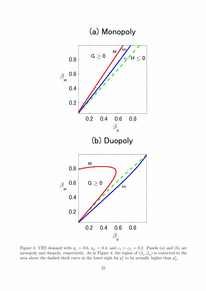
Figure 5: CES demand with ηs = 0.6, ηw = 0.4, and cs = cw = 0.2. Panels (a) and (b) aremonopoly and duopoly, respectively. As in Figure 4, the region of (βs, βw) is restricted to thearea above the dashed thick curve in the lower right for p∗s to be actually higher than p∗w.
25

where ωm > 0 is now the product-specific utility and βm > 0 is the responsiveness of the
representative consumer in market m to the price.27 Then, under symmetric pricing, each
firm’s share is
qm(p) =exp(ωm − βmp)
1 + 2 exp(ωm − βmp)
and the symmetric discriminatory equilibrium price p∗m = p∗m(cm, ωm, βm) satisfies:
p∗m − cm︸ ︷︷ ︸=µ∗m
− 1
βm(1− q∗m)= 0
and/∈q∗m ≡ qm(p∗m) =
exp(ωm − βmp∗m)
1 + 2 exp(ωm − βmp∗m).
Both p∗m and q∗m should be jointly solved numerically, and it is shown that
H(c,β,ω) =
(1− q∗w1− q∗s
)(βwβs− 1− 2q∗w
1− 2q∗s· 1− q∗s − [q∗s ]
2
1− q∗w − [q∗w]2
).
The equilibrium uniform price p = p(c,ω,β) satisfies∑m=s,w
qm(p) {1− βm(p− cm)[1− qm(p)]} = 0,
which should also be numerically solved. It is also verified that
G(c,β,ω) =p− csp− cw
− π′′s/q′s
π′′w/q′w
,
where,
π′′mq′m
=
2− Lm(p) · [ αownm (p)︸ ︷︷ ︸=βmp(1−2qm)
+ αcrossm (p)︸ ︷︷ ︸=βmp·qm(1−2qm)
1−qm
]
θm(p)︸ ︷︷ ︸=
1−2qm1−qm
− 1− θm(p)
θm(p)︸ ︷︷ ︸=
qm1−2qm
=2− 3qm1− 2qm
− βm(p− cm).
27Anderson, de Palma, and Thisse (1987) argue that the indirect utility of the representative consumer inmarket m is given by
Vm(pm) =ln [exp (ωm − βmpAm) + exp (ωm − βmpBm)]
βm.
This demand form can also be microfounded by the random utility model (see, e.g., Anderson, de Palma, andThisse 1992, Ch. 2).
26

Figure 6: Multinomial logit demand with ωs = 1.2, ωw = 0.8, and cs = cw = 0.2. Panels (a)and (b) are monopoly and duopoly, respectively. As in Figures 4, and 5, the region of (βs, βw)is restricted to the area above the dashed thick curve in the lower right for p∗s to be actuallyhigher than p∗w. The region for G ≥ 0 is the area above curve gg, whereas the region for H ≤ 0is the area between the dashed thick curve and curve hh.
27

Here, to see the role of the demand curvatures, we consider the region of (βs, βw), with a
fixed value of cs = cw = 0.2. Figure 6 shows that a higher value of βw, relative to βs, that
is, a higher degree of convexity in the weak market, is associated with a negative change in
social welfare by price discrimination. This result firstly appears not to be consistent with ACV
(2010), who emphasize that as the demand in the weak market becomes more convex, it is more
likely that price discrimination increases social welfare because a larger increase in output in the
weak market offsets the misallocation effect caused by price discrimination. However, ACV’s
(2010) result holds if the demand in the strong market is concave. Here, the demand in the
strong market is also convex. In this case, the uniform price is kept relatively low; thus an
introduction of price discrimination again highlights the misallocation effect.
5 Aggregate Output and Consumer Surplus
In this section, we extend our sufficient statistics approach to analysis of aggregate output as
well as consumer surplus.
5.1 Output Effects
First, we define hm(p) ≡ q′m(p)π′′m(p)
> 0 so that
Q′(t)
2=
(− π′′sπ
′′w
π′′s + π′′w
)︸ ︷︷ ︸
>0
{hw[pw(t)]− hs[ps(t)]} . (12)
and assume that this hm is increasing (and call it the increasing ratio condition for quantity;
IRCQ). This condition is equivalent to ςIm(p) > αIm(p), where ςIm(p) ≡ −dπ′′mdp
pπ′′m
= −pπ′′′mπ′′m
is the
industry-level price elasticity of π′′m and αIm(p) ≡ −pq′′mq′m
is the industry-level demand curvature.28
It is also expressed by νIm(p) > 0, where νIm(p) ≡ −ph′mhm
is the industry-level price elasticity of
28To see this, note that h′m < 0 is equivalent to π′′′m > (π′′mq′m
)q′′m, whereπ′′mq′m
> 0, because h′m(p) =π′′′mq
′m−π
′′mq′′m
(q′m)2 ,
which implies that:
h′m < 0⇔ −pπ′′′m
π′′m> −pq
′′m
q′m⇔ ςIm > αIm.
Essentially, the IRCQ states that the profit function, starting from the zero price, increases quickly, attainingthe optimal price, and then decreases slowly as p becomes larger and larger beyond the optimum. In this way,the optimal price is reached “close” enough to the zero price, rather than “still climbing up” even far away fromit. To see this, if q′′m > 0, then it is necessary for π′′′m to be positive. This means that π′′m, which is negative,should be larger (i.e., the negative slope of π′′m should be gentler) as p increases. If q′′m ≤ 0, then π′′′m should be,whether it is positive or negative, sufficiently large. In either case, as p increases, πm increases quickly belowthe optimum, and decreases slowly beyond it.
28

hm.29 Now, it is shown that
Q′′(t)
2=
(− q′sq
′w
π′′s + π′′w
)[h′sp
′s − h′wp′w] + [hs − hw]
d
dr
(− q′sq
′w
π′′s + π′′w
),
so that there exists t such that Q′(t) = 0 and Q′′(t)2
= − q′sq′w
π′′s+π′′w(h′sp
′s − h′wp
′w) < 0 because
h′sp′s < 0 and h′wp
′w > 0, implying the the global concavity of Q(t) is attained. Based on these
results, the following proposition is obtained.
Proposition 3. Given the IRCQ, if θ∗wρ∗w≥ θ∗sρ
∗s holds, the price discrimination increases
aggregate output. Conversely, ifθwρwθsρs
≤ π′′w(p)
π′′s(p)
holds, then price discrimination decreases aggregate output.
Proof. See Appendix, Part B.
Part C of the Appendix discusses the relationship between Holmes’ (1989) expression of the
output effect and ours, and interprets his result in terms of the sufficient statistics.
In a similar vein, Miklos-Thal and Shaffer (2021a) provide another sufficient condition for
price discrimination to increase aggregate output: θwρw > θsρs and ρw(1+θw) > ρs(1+θs) over
the relevant range. Obviously, if Miklos-Thal and Shaffer’s (2021a) sufficient condition holds,
our sufficient condition θ∗wρ∗w≥ θ∗sρ
∗s automatically holds because ours is a special case of theirs.
However, Miklos-Thal and Shaffer’s (2021a) sufficient condition must hold globally, whereas,
by imposing the IRCQ, we only require the condition to hold locally. Our sufficient condition
provides a prediction for when a change from the current regime decreases aggregate output
by using only the information available under the current regime: if price discrimination is
currently conducted and if θ∗wρ∗w≥ θ∗sρ
∗s holds, then banning price discrimination unambiguously
decreases aggregate output. Similarly, if the current regime is uniform pricing and θwρwθsρs≤ π′′w(p)
π′′s (p)
holds, then allowing price discrimination unambiguously decreases aggregate output.30
29This is because it is verified that
h′mhm
=π′′′mq
′m − π′′mq′′m[q′m]2︸ ︷︷ ︸<0
· q′m
π′′m︸︷︷︸>0
=π′′′mq
′m − π′′mq′′mq′mπ
′′m
,
and thus,
νIm =
(−pπ
′′′m
π′′m
)−(−pq
′′m
q′m
)= ςIm − αIm,
which implies that h′m < 0⇔ νIm > 0.30If hm is decreasing, as we assume throughout, then zm is increasing because
z′m(p) =1− zm(p)h′m(p)
hm(p)
29

5.2 Consumer Surplus
First, note that
CS ′(t)
2= ps(r) · q′s · p′s(t) + pw(t) · q′w · p′w(t)
−p′s(t)[ps(t) · q′s + qs]− p′w(t)[pw(t) · q′w + qw]
= −[p′s(t)qs + p′w(t)qw]
=
(− π′′sπ
′′w
π′′s + π′′w
)︸ ︷︷ ︸
>0
{gs[ps(t)]− gw[pw(t)]} , (13)
where gm(p) ≡ qm(p)π′′m(p)
. If gm is assumed to be decreasing, then one can use a similar argument.
We call this the decreasing marginal consumer loss condition (DMCLC), which is equivalent
to ςIm(p) > εIm(p).31 Then, the global concavity of CS(t) is attained. Thus, we can determine
the sign of CS ′(0): it follows that sign[CS ′(0)] = sign[ qs(p)π′′s (p)
− qw(p)π′′w(p)
], and thus, the following
proposition is obtained.
Proposition 4. Given the DMCLC, if the output in the weak market at the uniform price p is
so that z′m is positive if h′m is negative. That is, the IRCQ is a sufficient condition for the IRCW to hold.Thus, our IRCQ is a sophistication of ACV’s monotonicity condition (i.e., their IRC); it is a sophistication thatrequires “not too convex” demand functions to a stricter degree.
31Recall that ςIm(p) ≡ −dπ′′m
dppπ′′m
= −pπ′′′m
π′′mwas defined as the industry-level price elasticity of π′′m in Subsection
5.1 above. To see this relationship, note first that gm =q′mπ′′m· qmq′m = 1
hm× qm
q′m. Thus,
g′m = − h′m[hm]2
× qmq′m
+1
hm(1− σIm)
=1
hm[−(−ph
′m
hm
)︸ ︷︷ ︸
=νIm
(− qmpq′m
)︸ ︷︷ ︸
= 1
εIm
+ (1− σIm)],
where σIm(p) ≡ qmq′′m
[q′m]2 corresponds to what ACV (p. 1603) call the curvature of the the inverse demand., and it
is also written as:
σIm =
(−pq′′mq′m
)︸ ︷︷ ︸
=αIm
(− qmpq′m
)︸ ︷︷ ︸
= 1
εIm
=αImεIm
.
Hence, g′m = 1hm
[1− νIm+αIm
εIm
], which implies that g′m < 0 ⇔ νIm(p) + αIm(p) > εIm(p) ⇔ ςIm(p) > εIm(p).
it is also verified that g′m < 0 is equivalent to π′′′m >q′mπ
′′m
qm/, where the right hand side is positive, because
g′m =q′mπ
′′m−qmπ
′′′m
[π′′m]2. Now, recall that the IRCQ is equivalent to π′′′m >
q′′mπ′′m
q′m: if
q′mπ′′m
qm>
q′′mπ′′m
q′m/⇔ q′′m(p) <
[q′m(p)]2
qm(p) ,
that is qm(p) is not “too convex,” then the DMCLC is a sufficient condition for the IRCQ to hold. Thus, underthis “not too convex” assumption, the relationship, “DMCLC ⇒ IRCQ ⇒ IRCW,” holds if σIm(p) < 1 isadditionally imposed. The details are explained in Part E of the Online Appendix.
30

sufficiently large, i.e.,qw(p)
π′′w(p)≥ qs(p)
π′′s(p),
then price discrimination decreases consumer surplus.
Then, using profit margin and pass-through, we can rewrite Equality (13) as
CS ′(t)
2= (−π′′sπ′′w)︸ ︷︷ ︸
<0
(µw(t)ρw(t)
π′′w− µs(t)ρs(t)
π′′s
)
for t < t∗, and
CS ′(t∗)
2=
(− π′′sπ
′′w
π′′s + π′′w
)︸ ︷︷ ︸
>0
(µ∗wρ∗w − µ∗sρ∗s)
for t = t∗ which immediately leads to the following proposition.
Proposition 5. Given the DMCLC, if µ∗wρ∗w ≥ µ∗sρ
∗s holds, then price discrimination increases
consumer surplus. Conversely, ifµwρwµsρs
≤ π′′w(p)
π′′s(p)
holds, then price discrimination decreases consumer surplus.
Part F of the Online Appendix discusses whether the DMCLC holds in each of the three
parametric examples in Section 4 above.
6 Firm Heterogeneity
In this section, we argue that the main thrusts under firm symmetry also hold when heteroge-
neous firms are introduced. Without loss of generality, we keep considering one strong market
and one weak market. We also assume Corts’ (1998, p. 315) best response symmetry : all firms
agree on which market is strong and which market is weak. The case of best response asymmetry
is studied by Corts (1998) (see also Footnote 11 above).
The number of firms is N (≥ 2),32 and each firm j = 1, 2, ..., N has the constraint, pjs−pjw ≤tj. Then, as above, firm j’s price in the weak market under all of these constraints is written
32Here, all N firms are assumed to be present in both markets. This aspect of symmetry might be relaxed:the difference in the intensity of competition across the markets can also depend on the difference in the numberof active firms across them. For example, Aguirre (2019) shows that price discrimination increases aggregateoutput under linear demand either with Cournot competition or product differentiation if the number of firms inthe strong market is larger than that in the weak market. This counters the well-know result that in monopolyprice discrimination never changes aggregate output under linear demand (see, e.g., Robinson 1933; Schmalensee1981; Varian 1989). A similar finding is also obtained by Miklos-Thal and Shaffer (2021b) in the context ofintermediate price discrimination. We thank Inaki Aguirre for pointing this out to us.
31

as pjw(t) as a function of t = (t1, t2, ..., tN)T, where T denotes transposing. Accordingly, firm
j’s price in the strong market is written as pjs(t) = pjw(t) + tj. Therefore, the firms’ price pair
in market m = w, s is written as pm(t) = (p1m(t), p2m(t), ..., pNm(t))T. Then, social welfare is
defined as a function of t:
W (t) ≡ Us(xs[ps(t)]) + Uw(xw[pw(t)])− cTs · xs[ps(t)]− cT
w · xw[pw(t)],
where xm[pm(t)] = (x1m[pm(t)], x2m[pm(t)], ..., xNm[pm(t)])T and cm = (c1m, c2m, ..., cNm)T.33
Now, let t∗j ≡ p∗js − p∗jw for each j so that t∗ ≡ (t∗1, t∗2, ..., t
∗N)T. Then, each firm’s constraint
is written as 0 ≤ tj = λt∗j ≤ t∗j , with λ ∈ [0, 1]. Using this, we re-define the functions of t as
functions of one-dimensional variable, λ. In particular, the social welfare is written as:
W (λ) = Us(xs[ps(λ)]) + Uw(xw[pw(λ)])− cTs · xs[ps(λ)]− cT
w · xw[pw(λ)],
where pm can also be interpreted as a function of λ. Hence, the equilibrium uniform price is
written as p ≡ ps(0) = pw(0), whereas the equilibrium discriminatory prices are p∗s ≡ ps(1)
and p∗w ≡ pw(1).
We then use ∂xUm = pm from the representative consumer’s utility maximization problem
in each market m, where ∂xUm ≡(∂Um∂x1m
, ∂Um∂x2m
, ..., ∂Um∂xNm
), to derive
W ′(λ)︸ ︷︷ ︸1×1
=∑m=s,w
[µm(pm)T︸ ︷︷ ︸1×N
· (∂pmxm︸ ︷︷ ︸N×N
· p′m︸︷︷︸N×1
)],
where µm(pm) ≡ pm − cm is the profit margin vector,
∂pmxm ≡
(∂x1m∂p1m
...∂xNm∂p1m
︸ ︷︷ ︸≡∂p1mxm
. . .
∂x1m∂pNm
...∂xNm∂pNm
︸ ︷︷ ︸≡∂pNmxm
)
is the Jacobian for market demands, and p′m ≡ (p ′1m(λ), p ′2m(λ), ..., p ′Nm(λ))T.
33By allowing cost differences across firms and markets, Dertwinkel-Kalt and Wey (2020) study oligopolisticthird-degree price discrimination under the demand system proposed by Somaini and Einiv (2013), in whichdemand in each separate market is covered by all firms and thus no consumers are opting out. Under thisdemand system, Dertwinkel-Kalt and Wey (2020) show that each firm’s profit margin (i.e., the Lerner index)under uniform pricing is expressed as the weighted harmonic mean of its market-specific Lerner indices underprice discrimination. This result indicates that the profit margin is strictly lower the weighted arithmetic meanof the market-specific margins. In this sense, the market power measured by the Lerner concept is always lowerunder uniform pricing, and consumer surplus is strictly greater than under price discrimination. Note, however,that a change in social welfare is not an issue under this demand system because each firm’s output remainsthe same for both regimes.
32

Firm j’s profit function in market m = s, w is given by Equation (2), where pm now consists
of N firms’ prices as above, and
∂pjmπjm(pm) ≡ xjm(pm) + (pjm − cjm)∂xjm∂pjm
(pm)
is defined. Now, we apply the implicit function theorem to f(pw, λ) = 0, where
f( pw︸︷︷︸N×1
, λ︸︷︷︸1×1
) ≡
∂p1sπ1s(pw + λt∗) + ∂p1wπ1w(pw)...
∂pjsπjs(pw + λt∗) + ∂pjwπjw(pw)...
∂pNsπNs(pw + λt∗) + ∂pNwπNw(pw)
,
is a collection of all firms’ first-order conditions for profit maximization under regime λ, to
obtain p′w(λ) = −[Dpwf ]−1[Dλf ], where
Dpwf ≡
∂2π1s
∂p21s
+∂2π1w
∂p21w
· · · ∂2π1s
∂pNs∂p1s
+∂2π1w
∂pNw∂p1w...
. . ....
∂2πNs∂p1s∂pNs
+∂2πNw
∂p1w∂pNw· · · ∂2πNs
∂p2Ns
+∂2πNw∂p2
Nw
︸ ︷︷ ︸
≡K
=
∂2π1s
∂p21s
· · · ∂2π1s
∂pNs∂p1s...
. . ....
∂2πNs∂p1s∂pNs
· · · ∂2πNs∂p2
Ns
︸ ︷︷ ︸
≡Hs
+
∂2π1w
∂p21w
· · · ∂2π1w
∂pNw∂p1w...
. . ....
∂2πNw∂p1w∂pNw
· · · ∂2πNw∂p2
Nw
︸ ︷︷ ︸
≡Hw
and Dλf = Hst∗.
Here, the elasticity matrix and the curvature matrix can be defined by
εm =
ε11,m ε21,m · · · εN1,m
ε12,m ε22,m...
.... . .
...
ε1N,m ε2N,m · · · εNN,m
33

≡
− p1mx1m
∂x1m∂p1m
p1mx1m
∂x2m∂p1m
· · · p1mxNm
∂xNm∂p1m
p2mx1m
∂x1m∂p2m
− p2mx2m
∂x2m∂p2m
......
. . ....
pNmx1m
∂x1m∂pNm
· · · · · · − pNmxNm
∂xNm∂pNm
and
αm =
α11,m α21,m · · · αN1,m
α12,m α22,m...
.... . .
...
α1N,m · · · · · · αNN,m
≡
− p1m∂x1m∂p1m
∂2x1m∂p21m
− p2m∂x2m∂p2m
∂2x2m∂p2m∂p1m
· · · − pNm∂xNm∂pNm
∂2xNm∂pNm∂p1m
− p1m∂x1m∂p1m
∂2x1m∂p1m∂p2m
− p2m∂x2m∂p2m
∂2x2m∂p22m
...
.... . .
...
− p1m∂x1m∂p1m
∂2x1m∂p1m∂pNm
· · · · · · − pNm∂xNm∂pNm
∂2xNm∂p2Nm
,
respectively. Note also that for j = 1, 2, ..., N ,
∂2πjm(pm)
∂p2jm
= 2∂xjm∂pjm
(pm) + (pjm − cjm)∂2xjm∂p2
jm
(pm)
= −xjmpjm
(−pjmxjm
∂xjm∂pjm
)[2− pjm − cjm
pjm
(− pjm
∂xjm∂pjm
∂2xjm∂p2
jm
)]= − [2− Ljm(pjm)αjj,m] εjj,m
xjmpjm
and for j, k = 1, 2, ..., N , j 6= k,
∂2πjm(pm)
∂pjm∂pkm=
∂xjm∂pkm
(pm) + (pjm − cjm)∂2xjm
∂pjm∂pkm(pm)
=xjmpkm
(pkmxjm
∂xjm∂pkm
)1 +
(pkmpjm
)(pjm − cjm
pjm
) (− pjmxjm
∂xjm∂pjm
)(pkmxjm
∂xjm∂pkm
) (− pjm
∂xjm∂pjm
∂2xjm∂pjm∂pkm
)=
[1 +
(pkmpjm
)Ljm(pjm)
εjj,mεjk,m
αjk,m
]εjk,m
xjmpkm
,
which implies that Hs and Hw are expressed in terms of the sufficient statistics.
34

Now, we further proceed to obtain:p′w(λ) = [−K−1︸︷︷︸
N×N
Hs︸︷︷︸N×N
] t∗︸︷︷︸N×1
p′s(λ) = −K−1Hst∗ + t∗ =[I−K−1Hs︸ ︷︷ ︸
N×N
] t∗︸︷︷︸N×1
,
so that
W ′(λ) = [µTs ∂psxs][I−K−1Hs ]t
∗ − [µTw∂pwxw][K−1Hs ]t
∗
= {[µTs ∂psxs]K
−1[K−Hs ]− [µTw∂pwxw][K−1Hs ]}t∗
={(
[µTs ∂psxs]H
−1s
) (HsK
−1[K−Hs ])
−([µT
w∂pwxw]H−1w
) (HwK−1Hs
)}t∗.
Subsequently, we define
Zm(p) ≡ [µm(p)T∂pmxm(p)]︸ ︷︷ ︸1×N
H−1m (p)︸ ︷︷ ︸N×N
to proceed:
W ′(λ) = { Zw︸︷︷︸1×N
− Zs︸︷︷︸1×N
· (K−Hs)H−1w︸ ︷︷ ︸
N×N
}(−HwK−1Hs)t∗︸ ︷︷ ︸
N×1
= (Zw − Zs)(Γt∗),
where Γ ≡ −HwK−1Hs � 0 is assumed. We also assume that multi-dimensional version of
the IRC: for each market m and each firm j, Zjm is increasing in pl, l = 1, 2, ..., N .
We then define the multi-dimensional version of the conduct parameter (Weyl and Fabinger
2013, p. 552; see Footnote 16) by:
θm(p)T ≡(µm(p)T∂p1mxm(p)
−x1m(p). . .
µm(p)T∂pjmxm(p)
−xjm(p). . .
µm(p)T∂pNmxm(p)
−xNm(p)
)
35

as well as the pass-through matrix by:
ρm(λ) =
∂x1m∂p1m
(p) 0 · · · 0
0 ∂x2m∂p2m
(p) 0...
. . ....
0 0 · · · ∂xNm∂pNm
(p)
K−1(p) for λ < 1
∂x1m∂p1m
(p∗m) 0 · · · 0
0 ∂x2m∂p2m
(p∗m) 0...
. . ....
0 0 · · · ∂xNm∂pNm
(p∗m)
H−1m (p∗m) for λ = 1
as in the case of firm symmetry (recall the definition in Subsubsection 3.1.3).34
Hence, the three sufficient statistics under price discrimination are given by θ∗m ≡ θm(p∗m),
µ∗m ≡ µm(p∗m), and ρ∗m ≡ ρm(1). Similarly, those under uniform pricing are θm ≡ θm(p)
µm ≡ µm(p), and ρm ≡ ρm(0).
We are now able to generalizes Proposition 1 in the previous section for the case of firm
heterogeneity.
Proposition 6. Given the IRC, if [[θ∗w]T ◦ [µ∗w ]T]ρ∗w > [[θ∗s ]T ◦ [µ∗s ]
T]ρ∗s holds, where ◦ in-
dicates element-by-element multiplication, then price discrimination increases social welfare.
Conversely, if [[θw]T ◦ [µw ]T]ρw < [[θs ]T ◦ [µs ]
T]ρs∆, where ∆ ≡ K H−1
s HwK−1
is defined for
adjustment, where K ≡ K(p) and Hm ≡ Hm(p), m = s, w, holds, then price discrimination
decreases social welfare.
Proof. See Appendix, Part D.
Note that for each j, Z∗jm =∑N
k=1 θ∗kmµ
∗kmρ
∗jkm, which is interpreted as the weighted sum of
firm j’s own pass-through (ρ∗jjm) and the collection of its cross pass-through (ρ∗jkm, k 6= j). For
aggregate output and consumer surplus, we can readily generalize our previous results to the
case of firm heterogeneity in a similar manner by noting that
Q(λ) =N∑j=1
xjs[ps(λ)] +N∑j=1
xjw[pw(λ)]
34Given this definition, θm is rewritten as
θTm =
( ∑Nk=1 Lkmεk1,m
(−xkmx1m
). . .
∑Nk=1 Lkmεkj,m
(−xkmxjm
). . .
∑Nk=1 LkmεkN,m
(− xkmxNm
) ),
which implies that it can be expressed in terms of the sufficient statistics. Note also that ρm can be expressed
in terms of the sufficient statistics as well because∂xjm∂pjm
= −xjmpjm εjj,m holds for j = 1, 2, ..., N .
36

(a) Aggregate Output
If [θ∗w ]Tρ∗w > [θ∗s ]Tρ∗s , then Q∗ > Q.
If [θw]Tρw < [θs]Tρs∆, then Q∗ < Q.
(b) Social Welfare
If [[θ∗w]T ◦ [µ∗w ]T]ρ∗w > [[θ∗s ]T ◦ [µ∗s ]
T]ρ∗s , then W ∗ > W.
If [[θw]T ◦ [µw ]T]ρw < [[θs ]T ◦ [µs ]
T]ρs∆, then W ∗ < W.
(c) Consumer Surplus
If [µ∗w ]Tρ∗w > [µ∗s ]Tρ∗s , then CS∗ > CS.
If [µw ]Tρw < [µs ]Tρs∆, then CS∗ < CS.
Table 2: Summary of the Sufficient Conditions (with N heterogeneous firms, θm, µm , andρm are the conduct vector (N × 1), the profit margin vector (N × 1), and the pass-throughmatrix (N × N), respectively, in market m = s, w; asterisks and upper bars indicate pricediscrimination and uniform pricing, respectively; and ∆ is a term for adjustment defined in thetext).
and
CS(λ) = Us(xs[ps(λ)]) + Uw(xw[pw(λ)])− [ps(λ)]T · xs[ps(λ)]− [pw(λ)]T · xw[pw(λ)],
respectively. Table 2 summarizes our results for heterogeneous firms.
7 Concluding Remarks
This paper presents the theoretical implications of oligopolistic third-degree price discrimination
with general non-linear demand, allowing cost differentials to exist across separate markets. In
this sense, this paper, with the help of the methodology proposed by Weyl and Fabinger (2013),
synthesizes Aguirre, Cowan, and Vickers’ (2010) analysis of monopolistic third-degree price
discrimination with general demands and Chen and Schwartz’ (2015) analysis of monopolistic
differential pricing and extends them to the case of differentiated oligopoly.
Our theoretical analysis, which accommodates firm heterogeneity, can also be utilized to
empirically assess the welfare effects of third-degree price discrimination under oligopoly. In
particular, in line with the “sufficient statistics” approach (Chetty 2009), our predictions re-
garding the welfare effects do not rely on functional specifications, and are thus considered to
be fairly robust, although these sufficient statistics can take different values, depending on func-
tional specifications. However, once the numerical values of sufficient statistics are obtained,
37

there should be no disagreement regarding welfare assessment.
As a promising direction, it would be interesting to apply our methodology to the analysis
of the welfare effects of wholesale/input third-degree price discrimination (Katz 1987; DeGraba
1990; Yoshida 2000; Inderst and Valletti 2009; Villas-Boas 2009; Arya and Mittenforf 2010; Li
2014; O’Brien 2014; Gaudin and Lestage 2019; and Miklos-Thal and Shaffer 2021b).35 To do so,
one would need to properly define the sufficient statistics at each stage of a vertical relationship.
Another important issue to consider is the case of multi-product oligopolistic firms (Armstrong
and Vickers 2018; and Nocke and Schutz 2018). What happens if price discrimination is allowed
for some products, whereas uniform pricing is enforced for others? These and other important
issues related to third-degree price discrimination await further research.
Appendix
A. Proof of Proposition 1
Note first that
zm(pm) = −(pm − cm)εIm(pm)qm(pm)
pmπ′′m(pm)
= −θm(pm)qm(pm)
π′′m(pm)
holds. Now, define
F (pm, cm) =qm(pm)
∂xAm∂pA
(pm, pm)+ pm − cm
so that F (p∗m, cm) = 0 for m = s, w. Then, from the implicit function theorem, it is verified
that
ρm =1
1 +q′m
∂xAm/∂pA− qm
d (∂xAm/∂pA) /dpm
(∂xAm/∂pA)2
=∂xAm/∂pA
∂xAm∂pA
+ q′m −qm
∂xAm/∂pA
d
dpm
(∂xAm∂pA
) ,
and under the equilibrium discriminatory prices,
ρm(p∗m) =∂xAm(p∗m, p
∗m)/∂pA
q′m(p∗m) +∂xAm∂pA
(p∗m, p∗m) + (p∗m − cm)
d
dpm
(∂xAm∂pA
(p∗m, p∗m)
)35See Jaffe and Weyl (2013) for such an attempt.
38

=∂xAm(p∗m, p
∗m)/∂pA
π′′m(p∗m, cm),
which implies that
zm(p∗m) =
(−qm(p∗m)
∂xAm∂pA
(p∗m, p∗m)
)θm(p∗m)ρm(p∗m)
= µm(p∗m)θm(p∗m)ρm(p∗m)
and thusW ′(t∗)
2=
(− π′′sπ
′′w
π′′s + π′′w
)(µ∗wθ
∗wρ∗w − µ∗sθ∗sρ∗s) > 0
if µ∗wθ∗wρ∗w > µ∗sθ
∗sρ∗s holds. Given the IRC, this means that W (t) is strictly increasing in [0, t∗].
This completes the proof for the first part.
For t < t∗, note that
zm(pm) = θm
(−qm∂xAm∂pA
)(∂xAm∂pA
π′′m
)
= µmθm
(−
∂xAm∂pA
π′′s + π′′w
)︸ ︷︷ ︸
=ρm
(π′′s + π′′wπ′′m
).
Thus, it is verified that
W ′(t)
2= (−π′′sπ′′w)︸ ︷︷ ︸
<0
(µw(t)θw(t)ρw(t)
π′′w− µs(t)θs(t)ρs(t)
π′′s
),
which implies that given the IRC, W (t) is strictly decreasing in [0, t∗] if W ′(0) ≤ 0. This
completes the proof for the second part.
B. Proof of Proposition 2
First, note that q′mπ′′m
= θ∗m · ρ∗m. Then, this implies that from equality (12),
Q′(t)
2=
(− π′′sπ
′′w
π′′s + π′′w
)(θ∗wρ
∗w − θ∗sρ∗s) .
Conversely, for t < t, it can be verified that:
Q′(t)
2=
(q′w
∂xA,w∂pA
)(∂xA,w∂pA
)p′w +
(q′s
∂xA,s∂pA
)(∂xA,s∂pA
)p′s
39

= θw
( ∂xA,w∂pA
π′′s + π′′w
)(π′′s + π′′w)p′w + θs
( ∂xA,s∂pA
π′′s + π′′w
)(π′′s + π′′w)p′s
= (−π′′sπ′′w)︸ ︷︷ ︸<0
(θw(r)ρw(t)
π′′w− θs(r)ρs(t)
π′′s
).
C. Reinterpretation of Holmes’ (1989) Result on the Output Effects
in Terms of Sufficient Statistics
The following lemma holds when cost differentials are permitted.
Lemma. Q′(t) > 0 if and only if (suppressing the dependence on pm(t))
Lw ·αownw + αcrossw
θw− Ls ·
αowns + αcrosss
θs︸ ︷︷ ︸Adjusted-concavity
+1
θs− 1
θw︸ ︷︷ ︸Elasticity-ratio
> 0, (14)
where, following Holmes (1989), we call the first and the second terms in the left hand side of
inequality the adjusted-concavity part, and the third and the fourth terms the elasticity-ratio
part.
Proof. It is immediate to see that Q′(r)/2 is also given by
Q′(r)
2= q′w · p′w + q′s · p′s
= − π′′sq′w
π′′s + π′′w+
π′′wq′s
π′′s + π′′w
=
(− q′sq
′w
π′′s + π′′w
)︸ ︷︷ ︸
>0
(π′′sq′s− π′′wq′w
),
where (see Equation 7)
π′′m(p)
q′m(p)= {2− Lm(p)[αownm (p) + αcrossm (p)]} ε
ownm (p)
εIm(p)︸ ︷︷ ︸= 1θm(p)
− εcrossm (p)
εIm(p)︸ ︷︷ ︸=
1−θm(p)θm(p)
=2− Lm · (αownm + αcrossm )− (1− θm)
θm,
Hence,
Q′(r)
2=
(− q′sq
′w
π′′s + π′′w
)︸ ︷︷ ︸
>0
[(Lw ·
αownw + αcrossw
θw− 1
θw
)−(Ls ·
αowns + αcrosss
θs− 1
θs
)],
40

which completes the proof. This is also interpreted as a generalization of ACV’s (2010, p. 1608)
Equation (6).
Consider the adjusted-concavity part. A larger αownw and/or αcrossw make a positive Q′(r)
more likely. A larger αownw means that the firm’s own part of the demand in the weak market
(∂xA,w∂pA
) is more convex (“the output expansion effect”). Similarly, a larger αcrossw means that
how many of the firm’s customers switch to the rival’s product as a response to the firm’s price
increase is not so much affected by the current price level (“the countervailing effect”). In this
sense, the strategic concerns in the firm’s pricing are small. Thus, both a larger αownw and a
larger αcrossw indicate that the weak market is competitive. Even if∂xA,w∂pA
is not so convex, a
larger αcrossw can substitute it. Here, the intensity of market competition, 1/θw, magnifies both
effects, resulting in αownw
θwand αcrossw
θw. A similar argument also holds for αowns and αcrosss . In Part
D of the Online Appendix, we show that Holmes’ (1989) expression for Q′(r) (expression (9)
in Holmes 1989, p. 247) is equivalent to the left hand side of inequality (14) above.
D. Proof of Proposition 6
Using the definition of θm(p), we can rewrite:
Zm[pm(λ)] = [[θm [pm(λ)]]T︸ ︷︷ ︸1×N
◦ (−x1m[pm(λ)], ...,−xjm[pm(λ)], ...,−xNm[pm(λ)])︸ ︷︷ ︸1×N
]H−1m [pm(λ)]︸ ︷︷ ︸N×N
= [[θm [pm(λ)]]T◦[µm [pm(λ)]]T]
∂x1m∂p1m
[pm(λ)] 0 · · · 0
0 ∂x2m∂p2m
[pm(λ)] 0...
. . ....
0 0 · · · ∂xNm∂pNm
[pm(λ)]
H−1m [pm(λ)],
where
µm(p)T =
(−x1m(p)∂x1m∂p1m
(p). . .
−xjm(p)∂xjm∂pjm
(p). . . −xNm(p)
∂xNm∂pNm
(p)
)is used.
Then, for the first part of the proposition, it is immediate to see that
Zm(p∗m) = [[θm(p∗m)]T ◦ [µm(p∗m)]T]ρm(p∗m),
which is interpreted as a result of applying the implicit function theorem to g(pm , cm) = 0,
41

where
g( pm︸︷︷︸N×1
, cm︸︷︷︸N×1
) =
∂p1mπ1m(pm; c1m)...
∂p2mπjm(pm; c2m)...
∂pNmπNm(pm; cNm)
so that ρm(p∗m) = −[Dpmg]−1[Dcmg]. Now, note that W ′(1) > 0 if the inequality in this
proposition holds. Thus, given the IRC, W (λ) is strictly increasing in [0, 1], meaning that
social welfare is higher under price discrimination than under uniform pricing. This complete
the proof for the first part of the proposition.
For the second part, we proceed:
Zm(λ) = [[θTm ◦ µT
m ]ρm(λ)(KH−1m ),
for λ < 1, and thus
W ′(λ) ={
[θTw ◦ µT
w ]ρw [KH−1w K−1]− [θT
s ◦ µTs ]ρs [KH−1
s K−1]}
(KΓt∗)︸ ︷︷ ︸ .<<0
Then, it is verified that
W ′(0) < 0⇔ [θT
w ◦ µTw ]ρw [K H
−1
w K−1
] > [θT
s ◦ µTs ]ρs [K H
−1
s K−1
]
⇔ [θT
w ◦ µTw ]ρw < [θ
T
s ◦ µTs ]ρs [K H
−1
s K−1
][K H−1
w K−1
]−1
⇔ [θT
w ◦ µTw ]ρw < [θ
T
s ◦ µTs ]ρs [K H
−1
s HwK−1
],
which completes the proof.
References
Adachi, Takanori, and Michal Fabinger. 2021. “Pass-Through and the Welfare Effects of Tax-
ation under Imperfect Competition: A General Analysis.” Unpublished manuscript.
—, and Noriaki Matsushima. 2014. “The Welfare Effects of Third-Degree Price Discrimination
in a Differentiated Oligopoly.” Economic Inquiry, 52(3), 1231-1244.
Aguirre, Inaki. 2016. “On the Economics of the “Meeting Competition Defense” Under the
Robinson–Patman Act.” The B.E. Journal of Economic Analysis & Policy, 16(3), 1213-1238.
42

—. 2019. “Oligopoly Price Discrimination, Competitive Pressure and Total Out-
put.” Economics: The Open-Access, Open-Assessment E-Journal, 13 (2019-52). 1-16.
—, Simon Cowan, and John Vickers. 2010. “Monopoly Price Discrimination and Demand Cur-
vature.” American Economic Review, 100(4), 1601-1615.
Anderson, Simon P., Andre de Palma, and Jacques-Francois Thisse. 1987. “A Representative
Consumer Theory of the Logit Model.” International Economic Review, 29(3), 461-466.
—, —, and —. 1992. Discrete Choice Theory of Product Differentiation, The MIT Press.
Armstrong, Mark. 2006. “Recent Developments in the Economics of Price Discrimination.”
In: R. Blundell, W. Newey, and T. Persson (eds.), Advances in Economics and Econometrics:
Theory and Applications, Ninth World Congress, Vol. 2, Cambridge University Press, 97-141.
— 2008. “Price Discrimination.” In P. Buccirossi (ed.), Handbook of Antitrust Economics, The
MIT Press, 433-467.
—, and John Vickers. 2001. “Competitive Price Discrimination.” RAND Journal of Economics,
32(4), 579-605.
—, and —. 2018. “Multiproduct Pricing Made Simple.” Journal of Political Economy, 126(4),
1444-1471.
Arya, Anil, and Brian Mittenforf. 2010. “Input Price Discrimination when Buyers Operate in
Multiple Markets.” Journal of Industrial Economics, 58(4), 846-867.
Barnichon, Regis, and Geert Mesters. 2021. “Testing Macroeconomic Policies with Sufficient
Statistics.” Unpublished manuscript.
Boik, Andre. 2017. “The Empirical Effects of Competition on Third Degree Price Discrimination
in the Presence of Arbitrage.” Canadian Journal of Economics, 50 (4), 1023-1036.
Bresnahan, Timothy F. 1989. “Empirical Studies of Industries with Market Power.” In R.
Schmalensee and R. D. Willig (eds.), Handbook of Industrial Organization, Vol. 2, Elsevier
Science Publishers B.V., 1011-1057.
Chen, Yongmin, Jianpei Li, and Marius Schwartz. 2021. “Competitive Differential Pricing.”
RAND Journal of Economics, 52(1), 100-124.
—, and Marius Schwartz. 2015. “Differential Pricing When Costs Differ: A Welfare Analysis.”
RAND Journal of Economics, 46(2), 442-460.
43

Chetty, Raj. 2009. “Sufficient Statistics for Welfare Analysis: A Bridge Between Structural and
Reduced-Form Methods.” Annual Review of Economics, 1, 451-488.
Chone, Philippe, and Laurent Linnemer. 2020. “Linear Demand Systems for Differentiated
Goods: Overview and User’s Guide.” International Journal of Industrial Organization, 73,
102663.
Clerides, Sofronis K. 2004. “Price Discrimination with Differentiated Products: Definition and
Identification.” Economic Inquiry, 42(3), 402-412.
Corts, Kenneth S. 1998. “Third-Degree Price Discrimination in Oligopoly: All-Out Competition
and Strategic Commitment.” RAND Journal of Economics, 29(2), 306-323.
—. 1999. “Conduct Parameters and the Measurement of Market Power.” Journal of Economet-
rics, 88(2), 227-250.
Cowan, Simon. 2012. “Third-Degree Price Discrimination and Consumer Surplus.” Journal of
Industrial Economics, 60(2), 333-345.
—. 2016. “Welfare-Increasing Third-Degree Price Discrimination.” RAND Journal of Eco-
nomics, 47(2), 326-340.
—. 2017. “A Model of Third-Degree Price Discrimination with Positive Welfare Ef-
fects.” Unpublished manuscript.
—. 2018. “Regulating Monopoly Price Discrimination.” Journal of Regulatory Economics, 54(1),
1-13.
Dastidar, Krishnendu Ghosh. 2006. “On Third-Degree Price Discrimination in Oligopoly.” The
Manchester School, 74(2), 231-250.
Dertwinkel-Kalt, Markus, and Christian Wey. 2020. “Third-Degree Price Discrimination in
Oligopoly When Markets Are Covered.” Unpublished manuscript.
DeGraba, Patrick. 1990. “Input Market Price Discrimination and the Choice of Technology.”
American Economic Review, 80(5), 1246-1253.
De Loecker, Jan, Pinelopi K. Goldberg, Amit K. Khandelwal, and Nina Pavcnik. 2016. “Prices,
Markups and Trade Reform.” Econometrica, 84(2), 445-510.
Gaudin, Germain, and Romain Lestage. 2019. “Input Price Discrimination, Demand Forms,
and Welfare.” Unpublished manuscript.
44

Genesove, David, and Wallace P. Mullin. 1998. “Testing Static Oligopoly Models: Conduct and
Cost in the Sugar Industry, 1890-1914.” RAND Journal of Economics, 29(2), 355-377.
Hendel, Igal, and Aviv Nevo. 2013. “Intertemporal Price Discrimination in Storable Goods
Markets.” American Economic Review, 103(7), 2722-2751.
Holmes, Thomas J. 1989. “The Effects of Third-Degree Price Discrimination in Oligopoly.”
American Economic Review, 79(1), 244-250.
Hotelling, Harold. 1929. “Stability in Competition.” Economic Journal, 39(153), 41-57.
Inderst, Roman, and Tommaso Valletti. 2009. “Price Discrimination in Input Markets.” RAND
Journal of Economics, 40(1), 1-19.
Jaffe, Sonia, and E. Glen Weyl. 2013. “The First-Order Approach to Merger Analysis.” Amer-
ican Economic Journal: Microeconomics, 5(4), 188-218.
Katz, Michal L. 1987. “The Welfare Effects of Third-Degree Price Discrimination in Interme-
diate Goods Markets.” American Economic Review, 77(1), 154-167.
Kleven, Henrik J. 2021. “Sufficient Statistics Revisited.” Annual Review of Economics, 13,
515-538.
Leontief, W. 1940. “The Theory of Limited and Unlimited Discrimination.” Quarterly Journal
of Economics, 54(3), 490-501.
Li, Youping. 2014. “A Note on Third Degree Price Discrimination in Intermediate Good Mar-
kets.” Journal of Industrial Economics, 62(3), 554.
Melitz, Marc J. 2003. “The Impact of Trade on Intra-Industry Reallocations and Aggregate
Industry Productivity.” Econometrica, 71 (6), 1695-1725.
Miklos-Thal, Jeanine, and Greg Shaffer. 2021a. “Pass-Through as an Economic Tool: On Exoge-
nous Competition, Social Incidence, and Price Discrimination.” Journal of Political Economy,
129(1), 323-335.
—, and —. 2021b. “Third-Degree Price Discrimination in Oligopoly with Endogenous Input
Costs.” International Journal of Industrial Organization, Forthcoming.
Mrazova, Monika, and J. Peter Neary. 2017. “Not So Demanding: Demand Structure and Firm
Behavior.” American Economic Review, 107(12), 3835-3874.
Nahata, Babu, Krzysztof Ostaszewski, and P. K. Sahoo. 1990. “Direction of Price Changes in
Third-Degree Price Discrimination.” American Economic Review, 80(5), 1254-1258.
45

Nocke, Volker, and Nicolas Schutz. 2018. “Multiproduct-Firm Oligopoly: An Aggregative
Games Approach.” Econometrica, 86(2), 523-557.
O’Brien, Daniel P. 2014. “The Welfare Effects of Third-Degree Price Discrimination in Inter-
mediate Good Markets: The Case of Bargaining.” RAND Journal of Economics, 45(1), 92-115.
Pigou, Arthur C. 1920. The Economics of Welfare, Macmillan.
Quint, Daniel. 2014. “Imperfect Competition with Complements and Substitutes,” Journal of
Economic Theory, 152, 266-290.
Robinson, Joan. 1933. The Economics of Imperfect Competition, Macmillan.
Schmalensee, Richard. 1981. “Output and Welfare Implications of Monopolistic Third-Degree
Price Discrimination.” American Economic Review, 71(1), 242-247.
Schwartz, Marius. 1990. “Third-Degree Price Discrimination and Output: Generalizing a Wel-
fare Result.” American Economic Review, 80(5), 1259-1262.
Shapiro, Carl. 1996. “Mergers with Differentiated Products.” Antitrust, 10(2), 23-30.
Shubik, Martin, with Richard Levitan. 1980. Market Structure and Behavior, Harvard Univer-
sity Press.
Silberberg, Eugene. 1970. “Output under Discriminating Monopoly: A Revisit.” Southern Eco-
nomic Journal, 37(1), 84-87.
Somaini, Paulo, and Liran Einav. 2013. “A Model of Market Power in Customer Markets,”
Journal of Industrial Economics, 61(4), 938-986.
Stigler, George J. 1987. The Theory of Price, Fourth Edition, Macmillan.
Stole, Lars A. 2007. “Price Discrimination and Competition.” In M. Armstrong and R. Porter
(eds.), Handbook of Industrial Organization, Volume 1, Elsevier B.V., 2221-2299.
Varian, Hal R. 1985. “Price Discrimination and Social Welfare.” American Economic Review,
75(4), 870-875.
—. 1989. “Price Discrimination.” In R. Schmalensee and R. Willig (eds.), Handbook of Industrial
Organization, Volume 1, Elsevier B.V., 597-654.
Vickers, John. 2020. “Direct Welfare Analysis of Relative Price Regulation.” Journal of Indus-
trial Economics, 68(1), 40-51.
46

Villas-Boas, Sofia Berto. 2009. “An Empirical Investigation of the Welfare Effects of Banning
Wholesale Price Discrimination.” RAND Journal of Economics, 40(1), 20-46.
Vives, Xavier. 1999. Oligopoly Pricing: Old Ideas and New Tools, The MIT Press.
Weyl, E. Glen, and Michal Fabinger. 2013. “Pass-Through as an Economic Tool: Principle of
Incidence under Imperfect Competition.” Journal of Political Economy, 121(3), 528-583.
Yoshida, Yoshihiro. 2000. “Third-Degree Price Discrimination in Input Markets: Output and
Welfare.” American Economic Review, 90(1), 240-246.
47

Online Appendix
A. The Case of a General Number of Markets
Throughout this paper, we assume one strong market and one weak market. More gener-
ally, by defining S ≡ {m|p∗m > p} and W ≡ {m|p > p∗m}, we can let ps(r), s ∈ S, and
pw(r), w ∈ S, consist of the optimal price vector under constraints |pm − p| ≤ r for all
m ∈ S ∪ W , with r ∈ [0,maxm|p∗m − p|]. Then, for example, social welfare is defined as
W (r; cs, cw) ≡∑
s∈S Us(qs[ps(r)]) +∑
w∈W Uw(qw[pw(r)])− 2∑
s∈S(cs · qs[ps(r)])− 2∑
w∈W (cw ·qw[pw(r)]). Clearly, our two-market analysis does not lose any validity. In this way, an in-
crease in the weighted aggregate output,∑
m=s,w (p− cm) q′m[pm(r)]p′m(r) > 0, can be written as
E[(p−cm)q′mp′m] > 0 with a general number of markets. For this to hold, Cov(p−cm, q′mp′m) > 0,
that is, on average, the markup under uniform pricing and q′mp′m > 0 must be positively corre-
lated because E[(p− cm)] > 0 and E[q′mp′m] > 0.
B. Non-constant Marginal Costs
Notably, our analysis does not necessitate the assumption of no cost differentials between dis-
criminatory markets. In almost all theoretical studies on price discrimination, this assumption
is made mainly to focus on demand differences. However, in many real-world cases of price
discrimination, cost differentials are quite often observed, such as in the typical example of
freight charges across regional markets with different transportation and storage costs (Phlips
1983, pp. 5-7). In the narrowest definition of price discrimination, this might not be considered
price discrimination because they can be regarded as distinct products. However, airlines can
be arguably motivated to offer different types of seats because they seek to exploit hetero-
geneity among consumers. Thus, ideally, a theoretical analysis of price discrimination should
accommodate a moderate amount of cost differentials to exist across discriminatory markets.
Even if costs differ across markets, sellers may, in reality, have to engage in uniform pricing
due to the universal service requirement, fairness concerns from consumers or for other reasons
(Okada 2014; Geruso 2017; DellaVigna and Gentzkow 2019). In the case of monopoly with
differentials in marginal costs between markets, Chen and Schwartz (2015) derive sufficient
conditions under which the consumer surplus is higher under differential pricing.1 To ensure
that the strong market is indeed strong when cost differentials are allowed, it is sufficient to
assume that the marginal cost in the strong market, which is assumed to be a constant and
denoted by cs, is higher than in that in the weak market, cw: cs > cw (although cs should not
be too much higher than cw). Then, under uniform pricing, the profit margin in the strong
1Chen, Li and Schwartz (2021) extend Chen and Schwartz’ (2015) analysis to the case of oligopoly. See alsoGalera and Zaratiegui (2006) and Bertoletti (2009) as studies of conditions under which price discriminationincreases social welfare when cost differentials between markets are allowed.
48

market p − cs is smaller than that in the weak market p − cw. Differential pricing enables
the monopolist to sell more products in the weak market, which improves efficiency. Chen
and Schwartz (2015) discover that while differential pricing with no cost differentials (i.e.,
third-degree price discrimination in a traditional manner) tends to increase the average price
after differential pricing is permitted, differential pricing with cost differentials does not. In
contrast, our analysis provides welfare implications more directly. As in Chen and Schwartz
(2015), this paper does not make an explicit assumption regarding cs and cw as long as the
second-order conditions for profit maximization are satisfied and a sufficiently large discrepancy
between cw and cw does not change the order of discriminatory prices from the one with no
cost differentials.2
Notice that our results so far do not crucially depend on the assumption of constant marginal
costs. The only caveat is the definition of pass-through: to properly define pass-through in
accommodation with non-constant marginal costs, we introduce a small amount of unit tax
tm > 0 in market m: the firm’s first-order derivative of the profit with respect to its own price
(Equation 3 in the main text) is now replaced by
∂pπm(p) = qm(p) + (p− tm −mcm[qm(p)])∂xAm∂pA
(p, p),
where mcm = c′m[qm(p)] is the marginal cost at qm(p). Then, pass-through is defined by
ρm ≡ ∂pm∂tm
, and no other changes should be made to derive the results above. In fact, the
usefulness of pass-through is that it can easily be accommodated with non-constant marginal
costs (Weyl and Fabinger 2013; Fabinger and Weyl 2019; and Adachi and Fabinger 2021). An
additional caveat is that θ∗mρ∗m is no longer interpreted as quantity pass-through under price
discrimination (Weyl and Fabinger 2013, p. 572): one needs to take into account the “elasticity
of the marginal cost” to approximate the trapezoids of the welfare gain and loss by a deviation
from (full) price discrimination.
C. Computing the Sufficient Statistics Using the Parametric De-
mands
In this subsection, the number of firms is denoted by N ≥ 2.
2In the context of reduced-fare parking as a form of third-degree price discrimination with cost differentials,Flores and Kalashnikov (2017) characterize a sufficient condition for free parking (drivers receive a price discountin the form of complementary parking while pedestrians do not) to be welfare improving.
49

C.1 Linear Demand
When there are N symmetric firms, firm j’s direct demand in market m is given by
xjm =1
[1 + (N − 1)δm](1− δm)βm
{ωm(1− δm)− [1 + (N − 2)δm]pjm + δm
∑−jm
p−j,m
}.
In symmetric equilibrium, the firm’s demand in market m is qm(p) = qm(p) = ωm−p[1+(N−1)δm]βm
(and
thus, q′m(p) = − 1[1+(N−1)δm]βm
and εIm(p) = pωm−p) and the firm’s own price elasticity in market
m is
εownm (p) = − [1 + (N − 1)δm]βmωm − p
· p ·(− 1 + (N − 2)δm
[1 + (N − 1)δm](1− δm)βm
)=
[1 + (N − 2)δm]p
(1− δm)(ωm − p),
which implies that the discriminatory price in market m satisfies:
p∗m − cmp∗m
=(1− δm)(ωm − p∗m)
[1 + (N − 2)δm]p∗m
⇔ p∗m = p∗m(cm, ωm, δm) ≡ (1− δm)ωm + [1 + (N − 2)δm]cm2 + (N − 3)δm
.
and thus ρ∗m = 1+(N−2)δm2+(N−3)δm . Next, consider the uniform price. In symmetric equilibrium,
ymεownm =
ωm−p[1+(N−1)δm]βm∑
m=s,wωm−p
[1+(N−1)δm]βm
[1 + (N − 2)δm]p
(1− δm)(ωm − p)
=
[1+(N−2)δm]p[1+(N−1)δm](1−δm)βm∑m=s,w
ωm−p[1+(N−1)δm]βm
for m = s, w, which implies that the equilibrium uniform price p satisfies
∑m=s,w
[1 + (N − 2)δm](p− cm)
[1 + (N − 1)δm](1− δm)βm=∑m=s,w
ωm − p[1 + (N − 1)δm]βm
,
leading to the explicit solution:
p = p(c, δ,β,ω) ≡∑
m=s,w(1−δm)ωm+[1+(N−2)δm]cm
[1+(N−1)δm](1−δm)βm∑m=s,w
2+(N−3)δm[1+(N−1)δm](1−δm)βm
.
The conduct parameter in the case of linear demand is θm(pm) = pm−cmωm−pm . In each panel of
Figure OA1, the demand curve is depicted so that the ratio of (pm − cm) to (ωm − pm) takes
50

Figure OA1: θm with linear demands. In both cases, (pm− cm)/(ωm− pm) is almost identical.
almost the same value. However, in the left panel, the markup rate is high. This is mainly
due to a low elasticity of the industry’s demand rather than a low cross-price elasticity: the
rivalness between brands may be sufficiently high. In the right panel, the markup rate is low.
However, this does not necessarily mean that brands are in a strong rivalry. Instead,
εcrossm (pm) =pm
qm(pm)· ∂xBm∂pA
(pm, pm)
=[1 + (n− 1)δm]βmpm
ωm − pm· δm
[1 + (n− 1)δm](1− δm)βm
=δmpm
(ωm − pm)(1− δm)
can be low as long as εIm(pm) is sufficiently high (that εownm (pm) is high, and as a result, the
markup rate is low). In both panels, the market is close to monopoly because θm(pm) is close to
one. This graphical argument demonstrates that θm(pm), rather than Lm(pm), better captures
the competitiveness in market m. Because both the curvature of the firm’s direct demand and
the elasticity of the cross-price effect are zero (αownm (p) = 0 and αcrossm (p) = 0), it is observed
that
π′′m(p)
q′m(p)=
2− Lm(p) [αownm (p) + αcrossm (p)]− [1− θm(p)]
θm(p)
=1 + θm(p)
θm(p)
=ωm − cmp− cm
=2− δm1− δm
,
51

which implies that Q′(r) > 0 if and only if δs > δw, that is, the firms’ products are less differ-
entiated in the strong market. Finally, note that the following two restrictions are inevitably
imposed on the sufficient statistics: (i) the two curvatures, αownm and αcrossm , are necessarily zero,
and (ii) pass-through, ρm, is necessarily constant, and is always less than one (“cost-absorbing”).
Finally, in general (for N ≥ 2), it is verified that
G(c, δ,β,ω) =p− csp− cw
− [2 + (2N − 5)δs][1 + (N − 3)δw]
[2 + (2N − 5)δw][1 + (N − 3)δs]
and
H(c, δ,β,ω) =(ωs − cs)(1− δs)[2 + (N − 3)δw]
(ωw − cw)(1− δw)[2 + (N − 3)δs]− [2 + (N − 3)δs][1 + (N − 3)δw]
[2 + (N − 3)δw][1 + (N − 3)δs].
C.2 CES (Constant Elasticity of Substitution) Demand
The representative consumer’s utility in market m when there are N firms is given by
Um(xm) =
(N∑j=1
xβmjm
)ηm
.
Then, it is shown that
∂xAm∂pA
(p, p) = −N− 1−ηm
1−βmηm (βmηm)1
1−βmηm · [N − βm − (N − 1)βmηm]
N(1− βm)(1− βmηm)· p−
2−βmηm1−βmηm
and
d
dp
(∂xAm∂pA
(p, p)
)=N− 1−ηm
1−βmηm (βmηm)1
1−βmηm · [N − βm − (N − 1)βmηm](2− βmηm)
N(1− βm)(1− βmηm)2·p−1−
2−βmηm1−βmηm .
Similarly, it is observed that
qm(p) = N− 1−ηm
1−βmηm (βmηm)1
1−βmηm p−1
1−βmηm
and thus
q′m(p) = −N− 1−ηm
1−βmηm (βmηm)1
1−βmηm
1− βmηm· p−
2−βmηm1−βmηm
as well as
π′′m(p) = −N− 1−ηm
1−βmηm (βmηm)1
1−βmηm
N(1− βm)(1− βmηm)2· p−
2−βmηm1−βmηm
×{[N(2− βm)− βm − (N − 1)βmηm](1− βmηm)
52

−[N − βm − (N − 1)βmηm](2− βmηm) · p− cmp
}.
Therefore, the own price elasticity is given by the following constant :
εownm (p) = − p
qm(p)· ∂xAm∂pA
(p, p)
=N − βm − (N − 1)βmηmN(1− βm)(1− βmηm)
,
which indicates that the discriminatory price in market m is obtained explicitly by solving:
p∗m − cmp∗m
=N(1− βm)(1− βmηm)
N − βm − (N − 1)βmηm
⇔ p∗m = p∗m(cm, βm, ηm) ≡ [N − βm − (N − 1)βmηm]cmβm[(N − 1) + (1−Nβm)ηm]
.
Accordingly, the pass-through and the profit margin are given by:
ρ∗m =N − βm − (N − 1)βmηm
βm[(N − 1) + (1−Nβm)ηm]
and
µ∗m =N(1− βm)(1− βmηm)
βm[(N − 1) + (1−Nβm)ηm]cm
respectively, both of which are also constant.
Because it is shown that
∂xBm∂pA
(p, p) =N− 1−ηm
1−βmηm (βmηm)1
1−βmηm · βm(1− ηm)
N(1− βm)(1− βmηm)· p−1−
11−βmηm ,
the cross price elasticity is given by
εcrossm (p) =p
qm(p)· ∂xBm∂pA
(p, p)
=βm(1− ηm)
N(1− βm)(1− βmηm)
as a constant, which implies that the conduct is also given by
θ∗m = 1− (εcross)∗
(εown)∗=N − 2βm − (N − 2)βmηmN − βm − (N − 1)βmηm
as a constant.
53

The own and the cross curvatures are also obtained as constants:
αownm (p) =β2m(1− ηm)(2− ηm − βmηm) + (2− βm)N2(1− βmηm)2 − 3Nβm(1− ηm)(1− βmηm)
(1− βm)N(1− βmηm)[N(1− βmηm)− βm(1− ηm)]
and
αcrossm (p) = − βm(1− ηm)[N − 2βm − βmηm(N − 1− βm)]
(1− βm)N(1− βmηm)[N − βm − (N − 1)βmηm],
respectively.
The equilibrium uniform price satisfies
∑m=s,w
qm(p) ·[
[N − βm − (N − 1)βmηm](p− cm)
n(1− βm)(1− βmηm)− p]
= 0
because
ymεownm =
qm(p)
qs(p) + qw(p)· N − βm − (N − 1)βmηmN(1− βm)(1− βmηm)
.
It is also verified that
H(c,β,η) =
N(1− βs)(1− βsηs)csβs[(N − 1) + (1−Nβs)ηs]N(1− βw)(1− βwηw)cw
βw[(N − 1) + (1−Nβw)ηw]
−
1
N − 2βs − (N − 2)βsηsN − βs − (N − 1)βsηs
· N − βs − (N − 1)βsηsβs[(N − 1) + (1−Nβs)ηs]1
N − 2βw − (N − 2)βwηwN − βw − (N − 1)βwηw
· N − βw − (N − 1)βwηwβw[(N − 1) + (1−Nβw)ηw]
=βw[(N − 1) + (1−Nβw)ηw](1− βs)(1− βsηs)csβs[(N − 1) + (1−Nβs)ηs](1− βw)(1− βwηw)cw
−βs[(N − 1) + (1−Nβs)ηs][N − 2βw − (N − 2)βwηw]
βw[(N − 1) + (1−Nβw)ηw][N − 2βs − (N − 2)βsηs]
and
G(c,β,η)
=p− csp− cw
− (1− βw)(1− βwηw)
(1− βs)(1− βsηs)
×[N(2− βs)− βs − (N − 1)βsηs](1− βsηs)− [N − βs − (N − 1)βsηs](2− βsηs) ·
p− csp
[N(2− βw)− βw − (N − 1)βwηw](1− βwηw)− [N − βw − (N − 1)βwηw](2− βwηw) · p− cwp
54

because
π′′mq′m
=1
N(1− βm)(1− βmηm)
×{[N(2− βm)− βm − (N − 1)βmηm](1− βmηm)
−[N − βm − (N − 1)βmηm](2− βmηm) · p− csp
}.
C.3 Multinomial Logit Demand with Outside Option
When there are N symmetric firms, each firm j faces the following market share/demand
function:
xjm =exp(ωm − βmpjm)
1 +N∑j′=1
exp(ωm − βmpj′m)
,
and under symmetric pricing, each firm’s share is
qm(p) =exp(ωm − βmp)
1 +N · exp(ωm − βmp).
For any N ≥ 2, the own and cross price elasticities are εownm = βmpm(1 − qm) and εcrossm =
βmpmqm, respectively. Hence, the conduct parameter and the pass-through under price dis-
crimination are
θ∗m = 1− (εcrossm )∗
(εownm )∗=
1− 2q∗m1− q∗m
,
and
ρ∗m =1
1 +q∗m(1−N · q∗m)
(1− q∗m)2
,
respectively. It is thus shown that
H(c,β,ω) =
(1− q∗w1− q∗s
)(βwβs− 1− 2q∗w
1− 2q∗s· 1− q∗s − (N − 1)[q∗s ]
2
1− q∗w − (N − 1)[q∗w]2
).
Note here that under logit demand, pass-through, ρ∗m, is necessarily greater than one (“cost-
amplifying”).
Similar to the first-order elasticties, the two curvatures are expressed as αownm = βmpm(1−2qm) and αcrossm = βmpmqm(1−2qm)
1−qm for any N ≥ 2. Therefore, the expression for G(c,β,ω) cannot
become more complicated than that in the main text.
55

D. Equivalence of Holmes’ (1989) and Our Expressions for Q′(r) with
No Cost Differentials
Holmes (1989, p. 247), who assumes no cost differentials (c ≡ cs = cw) as in most of the
papers on third-degree price discrimination, also derives a necessary and sufficient condition
for Q′(r) > 0 under symmetric oligopoly. It is (using our notation) written as:
ps − cq′s(ps)
· ddps
(∂xA,s(ps, ps)
∂pA
)− pw − cq′w(pw)
· d
dpw
(∂xA,w(pw, pw)
∂pA
)︸ ︷︷ ︸
Adjusted-concavity condition (Robinson 1933)
+εcrosss (ps)
εIs(ps)− εcrossw (pw)
εIw(pw)︸ ︷︷ ︸Elasticity-ratio condition (Holmes 1989)
> 0.
Recall that 1θs− 1
θw= εcrosss
εIs− εcrossw
εIw. The first and the second terms in the left hand side of
Holmes’ (1989) inequality is rewritten as:
ps − cq′s(ps)
· ddps
(∂xA,s(ps, ps)
∂pA
)− pw − cq′w(pw)
· d
dpw
(∂xA,w(pw, pw)
∂pA
)= Lw(pw) ·
[(− pwq′w(pw)
)d
dpw
(∂xA,w(pw, pw)
∂pA
)]−Ls(ps) ·
[(− psq′s(ps)
)d
dps
(∂xA,s(ps, ps)
∂pA
)].
Now, it is also observed that
αownm + αcrossm
θm=
∂xAm/∂pAq′m
(− pm∂xAm/∂pA
∂2xAm∂p2A
− pm∂xAm/∂pA
∂2xAm∂pB∂pA
)= −pm
q′m
(∂2xAm∂p2A
+∂2xAm∂pB∂pA
).
=
(− pmq′m(pm)
)d
dpm
(∂xAm(pm, pm)
∂pA
).
Therefore, inequality (14) is another expression for Holmes’ (1989, p. 247) inequality (9) because
ps − cq′s· ddps
(∂xA,s∂pA
)− pw − cq′w(pw)
· d
dpw
(∂xA,w∂pA
)= Lw ·
αownw + αcrossw
θw− Ls ·
αowns + αcrosss
θs.
56

DMCLC: g′m < 0m
ςIm > εIm
⇓ (If σIm < 1 ⇔ εIm > αIm is imposed)
ςIm > αImm
IRCQ: h′m < 0
Table OA1: DMCLC implies IRCQ
E. An Alternative Way to Verify “DMCLC ⇒ IRCQ ⇒ IRCW”
First, recall that
g′m = − h′m[hm]2
× qmq′m
+1
hm(1− σIm),
where 1− σIm > 0 is assumed, that is, qm is not “ too convex.” Thus, g′m < 0 if and only if
h′m <
(q′mhmqm
)︸ ︷︷ ︸
<0
·(
1− qmq′′m
[q′m]2
)︸ ︷︷ ︸
>0
,
indicating that “if g′m < 0 (DMCLC), then h′m < 0 (IRCQ).” However, the converse is not true
because h′m < 0 is not sufficient to ensure that g′m < 0. This relationship is illustrated in Table
OA1.
Next, recall that zm(p) = (p− cm)/hm(p), which implies that
z′m =hm − (p− cm)h′m
[hm]2.
Thus, if h′m < 0, then hm > 0 > (p − cm)h′m, indicating that “if h′m < 0 (IRCQ), then z′m > 0
(IRCW).” However, the converse is not true because z′m > 0 is not sufficient to ensure that
h′m < 0.
F. Whether the DMCLC holds in the Parametric Examples
F.1 Linear Demand
First, it is observed that
π′′m(p) = q′m(p) +∂xAm∂pA
(p, p) + (p− cm)d
dp
(∂xAm∂pA
(p, p)
)
57

= − 1
(1 + δm)βm− 1(
1− δ2m)βm
= − 2− δm(1− δ2m)βm
< 0
because
q′m(p) = − 1
(1 + δm)βm
and∂xAm∂pA
(p, p) = − 1(1− δ2m
)βm
.
Then, it is verified that
gm(p) =qm(p)
π′′m(p)
=
(ωm−p
(1+δm)βm
)(− 2−δm
(1−δ2m)βm
)= −(ωm − p)(1− δm)
2− δm
and thus g′m(p) = 1−δm2−δm > 0; the DMCLC never holds. Moreover, the IRCQ does not hold,
either because
hm(p) =1
q′m(p)π′′m(p)
=
(− 2−δm
(1−δ2m)βm
)(− 1
(1+δm)βm
)=
2− δm1− δm
,
implying that h′m(p) = 0.
However, the IRCW does hold. This is because
zm(p) =(p− cm)q′m(p)
π′′m(p)
=(p− cm)
(− 1
(1+δm)βm
)(− 2−δm
(1−δ2m)βm
)= (p− cm)
(1− δm)
(2− δm),
58

which implies that z′m(p) = 1−δm2−δm > 0.
F.2 CES (Constant Elasticity of Substitution) Demand
First, it is verified that
π′′m(p) = −2− 1−ηm
1−βmηm (βmηm)1
1−βmηm
2(1− βm)(1− βmηm)2· p−
2−βmηm1−βmηm
×[(4− 3βm − βmηm)(1− βmηm)− (2− βm − βmηm)(2− βmηm) · p− cm
p
].
Then, it is observed that
gm(p) =qm(p)
π′′m(p)
= −2(1− βm)(1− βmηm)2
× [(4− 3βm − βmηm)(1− βmηm)p− (2− βm − βmηm)(2− βmηm)(p− cm)]
and thus
g′m(p) = −2βm(1− βm)(1− βmηm)2[(3− βm)ηm − βmη2m − 1],
which implies that gm is decreasing (the DMCLC) if and only if (3− βm)ηm − βmη2m − 1 < 0.
Figure A1 illustrates where the DMCLC holds in the region of (βm, ηm). However, the IRCQ
always holds because
hm(p) =1
q′m(p)π′′m(p)
=1
2(1− βm)(1− βmηm)
×[(4− 3βm − βmηm)(1− βmηm)− (2− βm − βmηm)(2− βmηm) · p− cm
p
]and thus
h′m(p) = −(2− βm − βmηm)(2− βmηm)cm2(1− βm)(1− βmηm)p2
< 0.
59

0.0 0.2 0.4 0.6 0.8 1.0
0.0
0.2
0.4
0.6
0.8
1.0
βm
ηm
DMCLC holds
Figure A1: The region for (βm, ηm) where the DMCLC holds under the CES demand.
F.3 Multinomial Logit Demand with Outside Option
Unfortunately, the DMCLC does not always hold for logit demand, though σIm(p) < 1 is
satisfied.3 To see this, first, recall that g′m < 0 if and only if ςIm > εIm (⇔ −pπ′′′mπ′′m
> −pq′mqm
), that
is,
−π′′′m(p)
π′′m(p)> βm · [1− 2qm(p)]⇔ π′′′m(p) > −βm · [1− 2qm(p)]π′′m(p),
where we derive (from Equations 2 and 3)
π′′m(p) = 2∂xAm∂pAm
(p, p) +∂xAm∂pBm
(p, p) + (p− cm)
[∂2xAm∂p2Am
(p, p) +∂2xAm
∂pBm∂pAm(p, p)
]= −βmqm(p)
{2− 3qm(p)− βm(p− cm)[1− 2qm(p)]2
}3To see this, recall that the logit demand under symmetric pricing is given by:
qm(p) =exp(ωm − βmp)
1 + 2 exp(ωm − βmp),
which implies that q′m(p) = −βmqm(p)[1− 2qm(p)] and q′′m(p) = −βmq′m(p)[1− 4qm(p)]. Hence,
q′′m(p) <[q′m(p)]2
qm(p)⇔ −βm[1− 4qm(p)] >
q′m(p)
qm(p)⇔ 1− 4qm(p) < 1− 2qm(p),
which must be true.
60

by using
∂xAm∂pAm
(p, p) = −βmqm(p)[1− qm(p)]
∂xAm∂pBm
(p, p) = βm[qm(p)]2
∂2xAm∂p2Am
(p, p) = β2mqm(p)[1− qm(p)][1− 2qm(p)]
∂2xAm∂pBm∂pAm
(p, p) = −β2m[qm(p)]2[1− 2qm(p)]
and
π′′′m(p) = 2∂2xAm∂p2Am
(p, p) + 3∂2xAm
∂pAm∂pBm(p, p) +
∂2xAm∂p2Bm
(p, p)
+(p− cm)
[∂3xAm∂p3Am
(p, p) + 2∂3xAm
∂p2Am∂pBm(p, p) +
∂3xAm∂pAm∂p2Bm
(p, p)
]= β2
mqm(p)[1− 2qm(p)] {2[1− 3qm(p)]
−βm(p− cm)[1− 2qm(p)][1− 6qm(p)]}
by additionally using
∂2xAm∂p2Bm
(p, p) = −β2m[qm(p)]2[1− 2qm(p)]
∂3xAm∂p3Am
(p, p) = −β3mqm(p)[1− qm(p)] {1− 6qm(p) + 6[qm(p)]2}
∂3xAm∂p2Am∂pBm
(p, p) = β3m[qm(p)]2 {1− 6qm(p) + 6[qm(p)]2}
∂3xAm∂pAm∂p
2Bm
(p, p) = β3m[qm(p)]2 {1− 4qm(p) + 6[qm(p)]2} .
Then, it is observed that
−βm[1− 2qm(p)]π′′m(p) = β2mqm(p)
×[1− 2qm(p)]{
2− 3qm(p)− βm(p− cm)[1− 2qm(p)]2},
which implies that
π′′′m(p) > −βm · [1− 2qm(p)]π′′m(p)
⇔ 2[1− 3qm(p)]− βm(p− cm)[1− 2qm(p)][1− 6qm(p)]
> 2− 3qm(p)− βm(p− cm)[1− 2qm(p)]2.
This is equivalent to βm(p − cm)[1 − 2qm(p)] > 3/4, and is not true for all p. In other words,
the DMCLC holds only when βm(p− cm)[1− 2qm(p)] > 3/4.
However, logit demand does satisfy the IRCQ (and hence the IRCW). This is because h′m
61

is negative if and only if ςIm > αIm (⇔ −pπ′′′mπ′′m
> −pq′′mq′m
), that is
π′′′m(p) > −βm · [1− 4qm(p)]π′′m(p)
⇔ [1− 2qm(p)] {2[1− 3qm(p)]− βm(p− cm)[1− 2qm(p)][1− 6qm(p)]}> [1− 4qm(p)] {2− 3qm(p)− βm(p− cm)[1− 2qm(p)]2} ,
which is further rewritten as βm(p− cm)[1− 2qm(p)]2 > −1/2, and this is obviously true.
References
Bertoletti, Paolo. 2009. “On the Output Criterion for Price Discrimination.” Economics Bul-
letin, 29(4), 2951-2956.
DellaVigna, Stefano, and Matthew Gentzkow. 2019. “Uniform Pricing in U.S. Retail Chains.”
Quarterly Journal of Economics, 134(4), 2011-2084.
Fabinger, Michal, and E. Glen Weyl. 2019. “Functional Forms for Tractable Economic Models
and the Cost Structure of International Trade.” Unpublished manuscript.
Flores, Daniel, and Vitaliy Kalashnikov. 2017. “Parking Discounts: Price Discrimination with
Different Marginal Costs.” Review of Industrial Organization, 50(1), 91-103.
Galera, Francisco, and Jesus M. Zaratiegui. 2006. “Welfare and Output in Third-Degree Price
Discrimination: A Note.” International Journal of Industrial Organization, 24(3), 605-611.
Geruso, Michael. 2017. “Demand Heterogeneity in Insurance Markets: Implications for Equity
and Efficiency.” Quantitative Economics, 8(3), 929-975.
Okada, Tomohisa. 2014. “Third-Degree Price Discrimination with Fairness-Concerned Con-
sumers.” The Manchester School, 86 (6), 701-715.
Phlips, Louis. 1983. The Economics of Price Discrimination, Cambridge University Press.
62