a study on stainless steel 316l annealed ultrasonic consolidation and linear welding density
TRANSCRIPT

Utah State UniversityDigitalCommons@USU
All Graduate Theses and Dissertations Graduate Studies
5-2010
A Study on Stainless Steel 316L AnnealedUltrasonic Consolidation and Linear WeldingDensity EstimationRaelvim GonzalezUtah State University
Follow this and additional works at: https://digitalcommons.usu.edu/etd
Part of the Mechanical Engineering Commons
This Thesis is brought to you for free and open access by the GraduateStudies at DigitalCommons@USU. It has been accepted for inclusion in AllGraduate Theses and Dissertations by an authorized administrator ofDigitalCommons@USU. For more information, please [email protected].
Recommended CitationGonzalez, Raelvim, "A Study on Stainless Steel 316L Annealed Ultrasonic Consolidation and Linear Welding Density Estimation"(2010). All Graduate Theses and Dissertations. 676.https://digitalcommons.usu.edu/etd/676

A STUDY ON STAINLESS STEEL 316L ANNEALED ULTRASONIC
CONSOLIDATION AND LINEAR WELDING
DENSITY ESTIMATION
by
Raelvim Gonzalez
A thesis submitted in partial ful�llmentof the requirements for the degree
of
MASTER OF SCIENCE
in
Mechanical Engineering
Approved:
Dr. Brent Stucker Dr. Leila LadaniMajor Professor Committee Member
Dr. David Geller Dr. Byron BurnhamCommittee Member Dean of Graduate Studies
UTAH STATE UNIVERSITYLogan, Utah
2010

ii
Copyright © Raelvim Gonzalez 2010
All Rights Reserved

iii
Abstract
A Study on Stainless Steel 316L Annealed Ultrasonic
Consolidation and Linear Welding
Density Estimation
by
Raelvim Gonzalez, Master of Science
Utah State University, 2010
Major Professor: Dr. Brent StuckerDepartment: Mechanical and Aerospace Engineering
Ultrasonic Consolidation of stainless steel structures is being investigated for potential
applications. This study investigates the suitability of Stainless Steel 316L annealed (SS316L
annealed) as a building material for Ultrasonic Consolidation (UC), including research on
Linear Welding Density (LWD) estimation on micrographs of samples. Experiment results
are presented that include the e�ect of UC process parameters on SS316L annealed UC,
optimum levels of these parameters, and bond quality of ultrasonically consolidated SS316L
annealed structures in terms of LWD. In support to these e�orts, a Measurement System
Analysis for LWD assessment has been performed, and a new instrument for LWD measure-
ment was developed. This work will determine local maximum LWD UC process parameters
for SS316L annealed structures based upon systematic evaluation of sample micrographs.
(116 pages)

iv
Acknowledgments
I would like to thank Utah State University PhD student Pedro J. Tejada, Utah State
University Professor Richard Cutler, and Indian Institute of Technology Professor G. D.
Janaki Ram for their valuable feedback and observations regarding the material outlined in
Chapter 2. In addition, the �nancial support received from the O�ce of Naval Research
(under Grant No. N000140710633) and �nancial and technical support from Solidica Inc. is
acknowledged and made the investigation presented in the Chapter 3 possible.

v
Contents
Page
Abstract . . . . . . . . . . . . . . . . . . . . . . . . . . . . . . . . . . . . . . . . . . . . . . . . . . . . . . . iii
Acknowledgments . . . . . . . . . . . . . . . . . . . . . . . . . . . . . . . . . . . . . . . . . . . . . . . . iv
List of Tables . . . . . . . . . . . . . . . . . . . . . . . . . . . . . . . . . . . . . . . . . . . . . . . . . . . vii
List of Figures . . . . . . . . . . . . . . . . . . . . . . . . . . . . . . . . . . . . . . . . . . . . . . . . . . viii
1 Introduction and Background . . . . . . . . . . . . . . . . . . . . . . . . . . . . . . . . . . . 1
1.1 Ultrasonic Consolidation . . . . . . . . . . . . . . . . . . . . . . . . . . . . . . 21.2 Linear Welding Density . . . . . . . . . . . . . . . . . . . . . . . . . . . . . . 51.3 E�ects of Process Parameters on UC Bond Formation . . . . . . . . . . . . . 61.4 Ultrasonic Consolidation System Description . . . . . . . . . . . . . . . . . . . 71.5 Research Goals . . . . . . . . . . . . . . . . . . . . . . . . . . . . . . . . . . . 71.6 Thesis Statement and Outline . . . . . . . . . . . . . . . . . . . . . . . . . . . 8
2 An Automatic Routine for Linear Welding Density Estimation through
Image Processing . . . . . . . . . . . . . . . . . . . . . . . . . . . . . . . . . . . . . . . . . . . . . . . . 12
2.1 Abstract . . . . . . . . . . . . . . . . . . . . . . . . . . . . . . . . . . . . . . . 122.2 Introduction . . . . . . . . . . . . . . . . . . . . . . . . . . . . . . . . . . . . . 122.3 Overview . . . . . . . . . . . . . . . . . . . . . . . . . . . . . . . . . . . . . . 132.4 Measurement System Analysis of Variance . . . . . . . . . . . . . . . . . . . . 192.5 Discussion . . . . . . . . . . . . . . . . . . . . . . . . . . . . . . . . . . . . . . 302.6 Summary and Conclusion . . . . . . . . . . . . . . . . . . . . . . . . . . . . . 362.7 Future Work . . . . . . . . . . . . . . . . . . . . . . . . . . . . . . . . . . . . 38
3 Experimental Determination of Optimum Parameters for Stainless Steel
316L Annealed Ultrasonic Consolidation . . . . . . . . . . . . . . . . . . . . . . . . . . . . . 42
3.1 Abstract . . . . . . . . . . . . . . . . . . . . . . . . . . . . . . . . . . . . . . . 423.2 Introduction . . . . . . . . . . . . . . . . . . . . . . . . . . . . . . . . . . . . . 423.3 Literature Review . . . . . . . . . . . . . . . . . . . . . . . . . . . . . . . . . . 463.4 Ultrasonic Consolidation System Description . . . . . . . . . . . . . . . . . . . 473.5 Experimental Work . . . . . . . . . . . . . . . . . . . . . . . . . . . . . . . . . 48
3.5.1 Experimental Units . . . . . . . . . . . . . . . . . . . . . . . . . . . . . 503.5.2 Taguchi Experiment . . . . . . . . . . . . . . . . . . . . . . . . . . . . 513.5.3 Split Plot Experiment and Analysis of Variance . . . . . . . . . . . . . 53
3.6 Discussion . . . . . . . . . . . . . . . . . . . . . . . . . . . . . . . . . . . . . . 703.7 Conclusion . . . . . . . . . . . . . . . . . . . . . . . . . . . . . . . . . . . . . . 733.8 Future Work . . . . . . . . . . . . . . . . . . . . . . . . . . . . . . . . . . . . 75

vi
4 Overall Conclusions . . . . . . . . . . . . . . . . . . . . . . . . . . . . . . . . . . . . . . . . . . . . 76
4.1 MATLAB Script for LWD Estimation through Image Processing . . . . . . . 764.2 Maximum LWD UC Parameters for SS316L Annealed UC . . . . . . . . . . . 784.3 Future Work . . . . . . . . . . . . . . . . . . . . . . . . . . . . . . . . . . . . 80
References . . . . . . . . . . . . . . . . . . . . . . . . . . . . . . . . . . . . . . . . . . . . . . . . . . . . . . 81
Appendix . . . . . . . . . . . . . . . . . . . . . . . . . . . . . . . . . . . . . . . . . . . . . . . . . . . . . . 85
A.1 MATLAB Script Supplement . . . . . . . . . . . . . . . . . . . . . . . . . . . 86A.1.1 How to Obtain the MATLAB Script . . . . . . . . . . . . . . . . . . . 86A.1.2 MATLAB Script User Guide . . . . . . . . . . . . . . . . . . . . . . . 86A.1.3 Known Limitations of the MATLAB Script . . . . . . . . . . . . . . . 93A.1.4 Step by Step MATLAB Script Visual Clicks Instructions . . . . . . . . 97A.1.5 MATLAB Script Original Code . . . . . . . . . . . . . . . . . . . . . . 99
A.2 Publication Permissions Supplement . . . . . . . . . . . . . . . . . . . . . . . 105

vii
List of Tables
Table Page
2.1 Factorial experiment Factors and Levels . . . . . . . . . . . . . . . . . . . . . 24
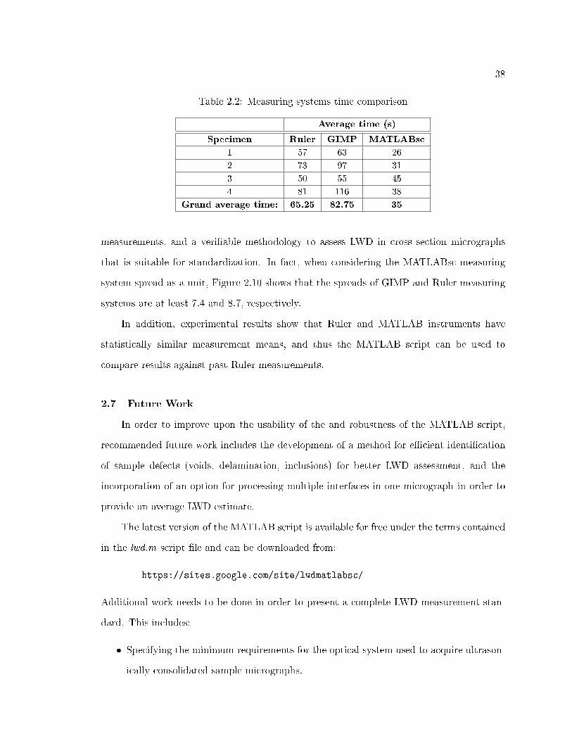
2.2 Measuring systems time comparison . . . . . . . . . . . . . . . . . . . . . . . 38
3.1 Sonotrode surface roughmess measurements . . . . . . . . . . . . . . . . . . . 48
3.2 Taguchi experiment Factors (UC process parameters) and Levels . . . . . . . 52
3.3 Taguchi L'16 experiment runs matrix . . . . . . . . . . . . . . . . . . . . . . . 53
3.4 Successful runs of the Taguchi experiment and corresponding LWD results . . 54
3.5 Split Plot experiment Factors (UC process parameters) and Levels, evaluatedat 478 K (400 °F) . . . . . . . . . . . . . . . . . . . . . . . . . . . . . . . . . 55
3.6 Split Plot experiment runs matrix . . . . . . . . . . . . . . . . . . . . . . . . . 65

viii
List of Figures
Figure Page
1.1 Schematic of the ultrasonic consolidation process [8] . . . . . . . . . . . . . . 3
1.2 Solidica Formation� machine at Utah State University (as shown in [12]) . . . 10
1.3 Solidica Formation� machine main elements (as shown in [11]) . . . . . . . . 10
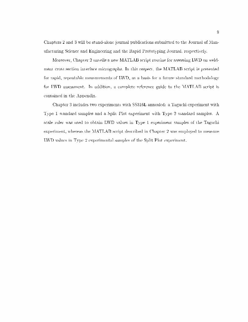
1.4 Close-up view of the Welding head, showing the sonotrode from below (asshown in [11]) . . . . . . . . . . . . . . . . . . . . . . . . . . . . . . . . . . . . 11
2.1 File input example in MATLAB script . . . . . . . . . . . . . . . . . . . . . . 14
2.2 Image, Interlayer Interface, and Region of Interest illustrations . . . . . . . . 15
2.3 Visual Clicks approach to de�ne the Region of Interest in the MATLAB script 16
2.4 8-bit grayscale conversion of the Region of Interest example in the MATLABscript . . . . . . . . . . . . . . . . . . . . . . . . . . . . . . . . . . . . . . . . 17
2.5 Illustration of black and white binarization using Otsu thresholding algorithmin the MATLAB script . . . . . . . . . . . . . . . . . . . . . . . . . . . . . . . 18
2.6 Illustration of black region vertical projection applied on a black and whiteimage in the MATLAB script . . . . . . . . . . . . . . . . . . . . . . . . . . . 19
2.7 MATLAB script output example . . . . . . . . . . . . . . . . . . . . . . . . . 20
2.8 The four randomized single-interface samples used for the Measurement Sys-tem Analysis (the sample labeled `Layer 2' was originally published in [7]) . . 22
2.9 Residuals versus Explanatory Factors before addressing heteroscedasticity . . 25
2.10 Box plots of the initial data showing high di�erences in Gage level variances . 26
2.11 Removed outliers as shown in Residuals vs Normal Percentiles plots for eachGage factor level . . . . . . . . . . . . . . . . . . . . . . . . . . . . . . . . . . 28
2.12 Residuals versus Explanatory Factors plots in �nal ANOVA . . . . . . . . . . 29
2.13 Residuals versus Predicted values plot in �nal ANOVA . . . . . . . . . . . . . 30

ix
2.14 Residuals vs Normal Percentiles plot for each Gage factor level in �nal ANOVA 31
2.15 Histogram for each Gage factor level in �nal ANOVA . . . . . . . . . . . . . . 32
2.16 Stem and Leaf plot and Boxplot for each Gage factor level in �nal ANOVA . 33
2.17 Type 3 �xed e�ects test and Least Squares Means for Gage factor in �nalANOVA . . . . . . . . . . . . . . . . . . . . . . . . . . . . . . . . . . . . . . . 34
2.18 Bad specimen preparation example . . . . . . . . . . . . . . . . . . . . . . . . 37
3.1 Schematic of the Ultrasonic Consolidation process [8] . . . . . . . . . . . . . . 43
3.2 Solidica Formation� machine (as shown in [11]) . . . . . . . . . . . . . . . . . 49
3.3 Close-up view of the Welding head, showing the sonotrode from below (asshown in [11]) . . . . . . . . . . . . . . . . . . . . . . . . . . . . . . . . . . . . 49
3.4 Base plate and part �xture in the Solidica Formation� machine (Left), andGeometry of the base plate showing bolt locations (Right) . . . . . . . . . . . 50
3.5 Schematic of a SS316L annealed Standard Sample (In Type 1: L =76.2 mm(3 inches), λ=63.5 mm (2.5 inches); In Type 2: L =63.5 mm (2.5 inches),λ=50.8 mm (2 inches)) . . . . . . . . . . . . . . . . . . . . . . . . . . . . . . . 51
3.6 Schematic of the SS316L annealed standard sample interfaces . . . . . . . . . 52
3.7 Micrograph of sample of Taguchi experiment run 6 . . . . . . . . . . . . . . . 55
3.8 Micrograph of sample of Taguchi experiment run 15 . . . . . . . . . . . . . . 56
3.9 Micrograph of sample of Taguchi experiment run 16 . . . . . . . . . . . . . . 57
3.10 Di�erent locations of the Position along the Welding Direction factor: at thebegining (b), in the middle (m), and at the end (e) . . . . . . . . . . . . . . . 58
3.11 Residuals versus Explanatory Factors plots for Split Plot ANOVA model . . . 61
3.12 Residuals versus Predicted values plot for Split Plot ANOVA model . . . . . . 62
3.13 Residuals vs Normal Percentiles plot for Split Plot ANOVA model . . . . . . 63
3.14 Histogram for each Gage factor level for Split Plot ANOVA model . . . . . . 64
3.15 Stem and Leaf plot and Boxplot for each Gage factor level for Split PlotANOVA model . . . . . . . . . . . . . . . . . . . . . . . . . . . . . . . . . . . 66
3.16 Type 3 �xed e�ects test results of the Split Plot ANOVA . . . . . . . . . . . . 67

x
3.17 Least Square Means table of the Split Plot ANOVA . . . . . . . . . . . . . . . 68
3.18 Di�erence of Least Square Means involving the optimum parameter set foundfor SS316L annealed UC in the Split Plot ANOVA . . . . . . . . . . . . . . . 69
3.19 Micrograph of Type 2 standard sample at the begining, made using Split Plotoptimum parameters (Normal Force=1800 N, Welding Speed=11 mm/s (26ipm), and Amplitude=27 µm, at 478 K (400 °F)) . . . . . . . . . . . . . . . . 71
3.20 Micrograph of Type 2 standard sample in the middle, made using Split Plotoptimum parameters (Normal Force=1800 N, Welding Speed=11 mm/s (26ipm), and Amplitude=27 µm, at 478 K (400 °F)) . . . . . . . . . . . . . . . . 72
3.21 Micrograph of Type 2 standard sample at the end, made using Split Plotoptimum parameters (Normal Force=1800 N, Welding Speed=11 mm/s (26ipm), and Amplitude=27 µm, at 478 K (400 °F)) . . . . . . . . . . . . . . . . 73
3.22 Least Squares Mean estimates for Normal Force, Welding Speed, and Ampli-tude factor levels . . . . . . . . . . . . . . . . . . . . . . . . . . . . . . . . . . 74
A.1 File input example in MATLAB script . . . . . . . . . . . . . . . . . . . . . . 87
A.2 Image, Interlayer Interface, and Region of Interest illustrations . . . . . . . . 88
A.3 Options menu to de�ne the Region of Interest in the MATLAB script . . . . . 88
A.4 Visual Clicks approach to de�ne the Region of Interest in the MATLAB script 89
A.5 Matrix Coordinates approach to de�ne the Region of Interest in the MATLABscript . . . . . . . . . . . . . . . . . . . . . . . . . . . . . . . . . . . . . . . . 90
A.6 Relative Coordinates approach to de�ne the Region of Interest in the MAT-LAB script . . . . . . . . . . . . . . . . . . . . . . . . . . . . . . . . . . . . . 91
A.7 Region of Interest example in the MATLAB script . . . . . . . . . . . . . . . 92
A.8 8-bit grayscale conversion of the Region of Interest example in the MATLABscript . . . . . . . . . . . . . . . . . . . . . . . . . . . . . . . . . . . . . . . . 93
A.9 Illustration of black and white binarization using Otsu thresholding algorithmin the MATLAB script . . . . . . . . . . . . . . . . . . . . . . . . . . . . . . . 94
A.10 Illustration of black region vertical projection applied on a black and whiteimage in the MATLAB script . . . . . . . . . . . . . . . . . . . . . . . . . . . 95
A.11 MATLAB script output example . . . . . . . . . . . . . . . . . . . . . . . . . 96
A.12 Bad specimen preparation example . . . . . . . . . . . . . . . . . . . . . . . . 98

1
Chapter 1
Introduction and Background
Previous research has shown that an additive manufacturing technique known as Ultra-
sonic Consolidation (UC), which produces three-dimensional structures from metal layers,
has been successfully utilized to consolidate Stainless Steel 316L layers [1]. However, from
a manufacturing process point of view, the understanding and knowledge needed for fabri-
cating SS316L annealed structures using UC requires information about the level of bond
quality expected in SS316L annealed consolidated specimens, and the ability to control the
e�ects of process parameters on SS316L annealed UC. This study addresses the critical issue
of optimizing process parameters for SS316L annealed UC based upon a maximum Linear
Welding Density criteria (minimum porosity), which is crucial knowledge for manufacturing
SS316L annealed parts, and for any application of SS316L annealed structures.
From an application standpoint, there are many reason for using SS 316L annealed
in combination with UC. By itself, Stainless Steel 316L is a common austenitic stainless
steel alloy, a general purpose marine grade material, and an attractive metal for structural
applications in a range of atmospheric environments [2, 3]. On the other hand, as a fabri-
cation method, UC has the advantages of being a low-temperature, metal based, computer-
controlled additive manufacturing process. These characteristics make UC a suitable tech-
nique to fabricate high tolerances/complex geometry parts, and to integrate components
into material structures in a single process; all while avoiding high temperature gradients in
metal parts. Since SS316L annealed is corrosion and pitting resistant, has better mechanical
strength than Aluminum (Al) � the typical material used in UC machines, and is widely
available in foil form (which makes it suitable for the UC process) it could be used in tandem
with UC to produce application-tailored structures with superior mechanical and corrosion
resistance.

2
Although the UC process of welding metal foils layer by layer is inherently aimed at
obtaining a continuum interface between layers, there is no standard procedure (conventions
in terms of magni�cation level, specimen preparation, measurement system, etc.) used for
Linear Welding Density (LWD) measurements, as of the time of this publication. For this
reason, this dissertation includes a �rst attempt at helping to create a standard LWD mea-
surement procedure, and evaluates a newly developed automatic routine for LWD assessment
that allows rapid, repeatable measurements, as a basis for a future standard methodology.
1.1 Ultrasonic Consolidation
Additive Manufacturing is a family of technologies for fabricating three-dimensional
(3D) structures directly from computer-aided design (CAD) data by means of systematic ad-
dition of material. Some of the potential bene�ts of the Additive Manufacturing approach in-
cludes the capability to build multi-material, functionally-graded, and component-embedded
structures [4]. Ultrasonic Consolidation (UC) is an additive manufacturing process whereby
layers of metal foils can be joined with a metallurgical bond by means of acoustic energy
and shaped using CNC machining.
As for the UC procedure, a computer program processes a three-dimensional CAD
model of the part to be built, and slices up this model into a number of horizontal layers,
each layer with a thickness equal to the thickness of the metal foil used. Ultrasonically
deposited foil strips are placed adjacently to each other to create a layer. After a layer is
completed (or several layers are completed), a computer controlled milling head shapes the
layer to its slice contour. Following this, milling chips are removed and foil deposition for
the next layer starts [5]. As a result of continuous addition of layers, a three-dimensional
part is produced from bottom to top.
A UC foil deposition schematic is shown in Figure 1.1. First, a thin metal foil is placed
over the substrate. Following this, a rotating ultrasonic sonotrode travels along the length
of the metal foil, keeping the foil in intimate contact with the substrate while a Normal
Force is applied to the metal foil through the sonotrode. The consolidation of the foil and
the substrate is accomplished by sonotrode oscillations at an ultrasonic frequency and at

3
user-set amplitude. The direction of the sonotrode's oscillations (direction of excitation) is
along the sonotrode's rotation axis.
As a consequence of sonotrode dynamics, localized shear forces are generated from the
combination of sonotrode pressure and oscillation, inducing interfacial stresses between the
two mating surfaces and elastic-plastic deformation of surface asperities [6]. Furthermore,
asperities deformations break up the oxide �lm, establishing a metallurgical bond between
the foil and the substrate due to relatively clean metal-to-metal surface contact [5]. On a
lower scale, atomic di�usion may also aid in the bonding process because local temperatures
at the interface and the surrounding a�ected region (about 20 µm) can reach up to 50%
of the melting point of the material being deposited [6], but only for a very brief time.
Although still being researched, there is evidence that ultrasonic welding mechanisms for
bond formation involve: i) removal of surface oxide layers, ii) plastic deformation at the
interface, and iii) to a lesser extent di�usion of metal atoms across the interface. The
degree of plastic deformation is considered the most important characteristic leading to
metallurgical bonding across the interface [7].
Although localized frictional heating is present in the UC process, the mechanism for
UC is not melting [6], and thus negligible shrinkage and thermal stresses result during part
building. In turn, ultrasonically consolidated parts have virtually no thermal degradation in
material properties. Indeed, parts may be built including complex geometric features (e.g.
internal channels) and integrating sensors/actuators for application-tailored structures, on
Fig. 1.1: Schematic of the Ultrasonic Consolidation process [8]

4
account of UC being an additive manufacturing process. Through ultrasonic welding and
CNC machining combined in an additive/subtractive manufacturing scheme, the UC process
can be used to create multi-material structures utilizing cold-working while avoiding thermal
processes that pose properties degradation [5]. In addition to this, UC does not require a
controlled atmosphere for layer deposition.
There are four general control parameters for welding within a UC system: Oscilla-
tion Amplitude, Contact Pressure Distribution (Normal Force between the horn and foil),
Welding Speed along the direction of travel, and Temperature of the substrate. The �rst
three parameters depend on sonotrode interaction with the part being built. In contrast,
Temperature depends on the heat applied directly to the substrate from the base plate, with
Temperature values from room temperature up to hundreds of kelvin degrees, typically 478
K (400 °F).
Evaluation of the e�ect UC control parameters have on microstructure and mechanical
properties of ultrasonically consolidated parts has been the object of active research [9] [10].
Regarding the object of study of the present thesis project, previous research has demon-
strated the feasibility of the UC process using Stainless Steel 316L by exploring the role
played by process parameters of Welding Speed, amplitude, Normal Force, and Tempera-
ture in Stainless Steel ultrasonic consolidation, and presenting optical microscopy of SS316L
ultrasonically consolidated samples [1]. Previous results of an Analysis of Variance (ANOVA)
on SS316L UC, with peel strength as the response and amplitude, Normal Force, and Weld-
ing Speed as factors, indicated that only amplitude and Welding Speed factors were sta-
tistically signi�cant for peel strength (with a 90% con�dence interval, p-value < 0.10). In
addition, according to this study, the amplitude factor exerted the strongest e�ect on peel
strength [1]. Furthermore, as for the e�ect of process parameters on peel strength, higher
Oscillation Amplitudes and lower Welding Speed increased peel strength. Normal force (up
to 1600 N) was not statistically signi�cant, whereas Temperature (up to 422 K (300°F)) was
not considered as a factor for SS316L UC [1].

5
1.2 Linear Welding Density
Linear Welding Density (LWD) is the proportion of bonded area to total area within
the weld interface [9]. The selection of LWD as a quality measure is better understood
considering that ultrasonically consolidated parts typically show unbonded regions (defects,
physical discontinuities) along the layer interfaces. Indeed, the assessment of the propor-
tional bonded region given in a LWD measurement is also important as a quality attribute
for porosity in ultrasonically consolidated parts [11]. The relevance of understanding what
factors in�uence LWD has already been observed in a previous study of UC parts [7]. As
a matter of fact, LWD strongly a�ects mechanical properties in the direction normal to the
foils for an ultrasonically consolidated part and the mechanical behavior of a UC structure
under load-bearing stresses [7]. In consequence, properties like speci�c weight and Poisson's
ratio of ultrasonically consolidated parts are a�ected by LWD. In the same manner, quality
charateristics based on ultrasonically consolidated part porosity (e.g. insulating enclosures)
are utterly dependent upon the level of LWD present between metal foils.
For the purposes of this thesis project, LWD will be determined based upon metallogra-
phy of the weld interface, by sectioning weld samples along the width of the foil. The samples
will be mounted, polished to a smooth �nish and cleaned in isopropyl alcohol. LWD will
be assessed from micrograph images of samples taken from weld cross-sections, according to
Equation (1.1).
%LWD =Bonded interface length
Total interface length× 100 (1.1)
Regarding methods that have been used for assessing LWD on ultrasonically consol-
idated samples, manual distance measuring instruments (e.g. rulers, software measuring
tools) have been used to estimate both the bonded interface length and the total interface
length in Equation 1.1. However, these methods have some inherent limitations and di�-
culties with LWD measurements, because they are time consuming, prone to human errors,
and impractical for accuracy veri�cation.

6
1.3 E�ects of Process Parameters on UC Bond Formation
In a UC system, the controllable variables for a given material are: Amplitude of
Oscillation, Contact Pressure distribution (Normal Force between the horn and foil), Welding
Speed (along direction of travel) and Temperature of the base. Extensive experimental
investigations have been conducted, studying the e�ects of these factors on the quality of
weldment made by UC.
Considering research made on Al 3003/6001, a higher Normal Force and higher Oscil-
lation Amplitude increased LWD up to a certain level, beyond which LWD decreased [9,10].
Additionally, it was observed that lower Welding Speeds (down to 12 mm/s) increase LWD,
and higher temperatures produced higher LWD within a range from ambient to 450 K (350
°F) [7]. Based on these studies, Al 3003 UC seems to be sensitive to changes in Oscillation
Amplitude values and substrate temperature.
Selection of appropriate process parameters plays a key role in UC bond formation of Al
3003/6061 based on LWDmicroscopic studies and peel-o� tests [9,10]. Although it is possible
to have a low peel load response and high linear weld density with Aluminum 6061 (due to
excessive strain hardening and cyclical stressing of contact points at the interface) [9]; it has
been veri�ed that a high peel load response only occurs in the presence of high LWD [10].
Current published literature about SS316L UC only comprises a paper studying the
feasibility of the UC process with SS316L, and exploring the e�ects of Amplitude, Normal
Force, and Welding Speed UC process parameters on peel strength by performing an ANOVA
study [1]. However, the e�ect of temperatures higher than 422 K (300 °F) was not part of
the study, and the benchmark used to characterize ultrasonically consolidated parts was
peel strength, instead of LWD. Considering these research e�orts, a study of parameter
optimization of SS316L annealed UC based on a maximum LWD criteria does not have
any precedent in literature. Moreover, a broader spectrum of UC parameter sets might
contribute to a better optimization of the SS316L annealed UC process with respect to a
maximum LWD criteria. In sum, an understanding of the e�ect of UC process parameters
on LWD is required if the SS316L UC is to develop its full application potential.

7
1.4 Ultrasonic Consolidation System Description
The UC system utilized for the experimental part of this thesis research is the So-
lidica Formation� machine. The Solidica Formation� UC machine (Figure 1.2, Figure 1.3,
and Figure 1.4) is an integrated UC building system that combines a rotating ultrasonic
sonotrode, a heat plate, a foil-feeding spool mechanism, a three-axis milling head, and a
software implementation for material deposition and machining [11]. Furthermore, the So-
lidica Formation� sonotrode oscillates transversely according to a half-wave recti�ed sine
wave at a frequency of 20 kHz and at user-set Oscillation Amplitude while traveling over the
metal foil. The sonotrode itself is incorporated into a welding head and its position is con-
trolled by numerical control. The maximum build size of the Solidica Formation� machine
is 609.6 mm × 914.4 mm × 203.2 mm (24 in × 36 in × 8 in), and the CNC contour milling
head has a tolerance of 0.05 mm (0.002 in) [12]. The sonotrode has a 146.75 mm nominal
diameter. Regarding process parameter setting limits, the Solidica Formation� machine is
constrained by the manufacturer to a nominal force less than or equal to 1800 N, nominal
amplitudes between 6 µm and 27 µm, Welding Speeds up to 84.7 mm/s (200 ipm), and
nominal temperatures ranging from ambient to 478 K (400 °F).
1.5 Research Goals
This is a systematic study exploring the suitability of Stainless Steel 316L annealed
(SS316L annealed) as a building material for Ultrasonic Consolidation (UC), including re-
search on Linear Welding Density (LWD) estimation on micrographs of samples. The re-
search is devoted to exploring the capabilities of ultrasonic consolidation to fabricate integral
SS316L annealed structures with maximum LWD, based upon systematic evaluation of LWD
estimation procedures. The objectives of this thesis project are to:
1. Develop a standard measurement system for LWDmeasurements, and evaluate SS316L
annealed UC bonding in specimens using LWD values as the response variable.

8
2. Determine the optimum LWD process parameter set for SS316L annealed UC experi-
mentally, and determine the e�ect of UC process parameters on the LWD of ultrason-
ically consolidated SS316L annealed structures.
As a result of these goals, a set of experimental and analytical studies were conducted
to develop a repeatable methodology for LWD measurements, and an Analysis of Variance
was performed to determine critical process parameters for Stainless Steel 316L annealed
Ultrasonic Consolidation. All these e�orts provide information related to the level of Linear
Welding Density attainable in SS316L annealed structures.
1.6 Thesis Statement and Outline
This study addresses parameter optimization for ultrasonic consolidation of Stainless
Steel 316L annealed, by evaluating experimental factors of Oscillation Amplitude, Welding
Speed, Normal Force and Temperature in order to minimize part porosity and therefore,
on the basis of a maximum LWD criteria. This thesis project will be presented in a multi-
paper format, in accordance with the requirements set by the Graduate School of Utah
State University. This study will include an introduction, background, and conclusion in
addition to the main chapters. The main body will consist of papers that have already been
published or already submitted for publication. In that respect, the outline of thesis project
is structured as follows:
� Chapter 1: Introduction and Background.
� Chapter 2: An automatic routine for Linear Welding Density estimation through image
processing.
� Chapter 3: Experimental determination of optimum parameters for stainless steel 316L
annealed ultrasonic consolidation.
� Chapter 4: Overall Conclusions.
� Appendix.
9
Chapters 2 and 3 will be stand-alone journal publications submitted to the Journal of Man-
ufacturing Science and Engineering and the Rapid Prototyping Journal, respectively.
Moreover, Chapter 2 unveils a new MATLAB script routine for assessing LWD on weld-
ment cross section interface micrographs. In this respect, the MATLAB script is presented
for rapid, repeatable measurements of LWD, as a basis for a future standard methodology
for LWD assessment. In addition, a complete reference guide to the MATLAB script is
contained in the Appendix.
Chapter 3 includes two experiments with SS316L annealed: a Taguchi experiment with
Type 1 standard samples and a Split Plot experiment with Type 2 standard samples. A
scale ruler was used to obtain LWD values in Type 1 experiment samples of the Taguchi
experiment, whereas the MATLAB script described in Chapter 2 was employed to measure
LWD values in Type 2 experimental samples of the Split Plot experiment.

10
Fig. 1.2: Solidica Formation� machine at Utah State University (as shown in [12])
Fig. 1.3: Solidica Formation� machine main elements (as shown in [11])
11
Fig. 1.4: Close-up view of the Welding head, showing the sonotrode from below (as shownin [11])
12
Chapter 2
An Automatic Routine for Linear Welding Density Estimation
through Image Processing1
2.1 Abstract
Linear Welding Density (LWD) is a quality benchmark used in ultrasonically consol-
idated part characterization. In this study, a computer-based method for assessing LWD
is presented. A MATLAB script is employed for assessing LWD on weldment cross section
interface micrographs. The method presented is based upon the application of image pro-
cessing techniques on a single metal to metal interface picture for LWD assessment, using
a picture brightness criteria. A Measurement System Analysis of Variance was performed
in order to evaluate repeatability and reproducibility of the MATLAB script presented in
this work against other conventional instruments used for LWD estimation. The experimen-
tal results presented show that the MATLAB script can e�ectively estimate LWD on cross
section micrographs.
2.2 Introduction
Ultrasonic Consolidation (UC) is an additive manufacturing process whereby layers of
metal foils can be joined with a metallurgical bond by means of acoustic energy and shaped
using CNC machining. Some of the UC process advantages are the ability to create metal
structures with virtually no thermal degradation in material properties [6] and include some
complex geometric features in metal parts (e.g. embedded sensors/actuators), all by taking
1Coathored by R. Gonzalez, B. Stucker. This chapter is a paper that has been submitted for publication
in the Journal of Manufacturing Science and Engineering.

13
advantage of the additive manufacturing nature of the process. The process of welding metal
foils layer by layer is inherently aimed at obtaining a continuum interface between layers.
Although perfect bonding is theoretically possible, ultrasonically consolidated parts typically
show unbounded regions in the form of defects, physical discontinuities, and imperfections
[11]. In that sense, Linear Welding Density (LWD) is de�ned by the proportion of bonded
area to total area within the weld interface [9]. For instance, LWD measurements have been
used to characterize bond quality in Al 3003 ultrasonically consolidated parts [7,13]. In turn,
it has been noted that LWD is directly related to porosity in ultrasonically consolidated
parts [11], strongly a�ects mechanical properties in the direction normal to the foils in an
ultrasonically consolidated part, and is an important factor to determine the mechanical
behavior of ultrasonically consolidated parts under load-bearing stresses [7].
Given a cross section micrograph, the LWD of a given interface is measured using a
relation of lengths given by the following equation:
%LWD =Bonded interface length
Total interface length× 100 (2.1)
As of the time of this publication, there is no standard procedure (conventions in terms
of magni�cation level, specimen preparation, measurement system, etc.) used for LWD mea-
surements. This paper is a �rst attempt at helping to create a standard LWD measurement
procedure. Indeed, this study presents a MATLAB script capable of assessing LWD given
an image containing the interface between two layers and compares results with other LWD
assessment methods on the basis of an Analysis of Variance (ANOVA).
2.3 Overview
A MATLAB script, `lwd.m', was developed to assess LWD in cross section micrographs
of weldments. The method is based upon the use of a set of image processing techniques
that, when combined, provide a single metal to metal interface LWD assessment. The
MATLAB script takes for an input a rectangular region of the cross section micrograph, and
provided this region contains the interface of interest and meets standard metallography
14
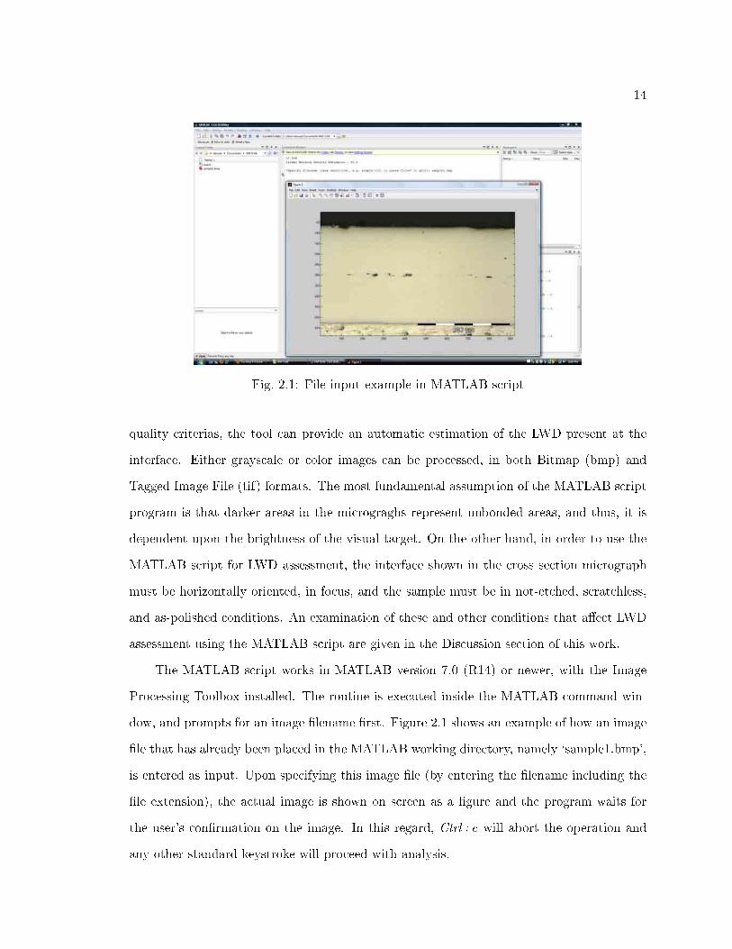
Fig. 2.1: File input example in MATLAB script
quality criterias, the tool can provide an automatic estimation of the LWD present at the
interface. Either grayscale or color images can be processed, in both Bitmap (bmp) and
Tagged Image File (tif) formats. The most fundamental assumption of the MATLAB script
program is that darker areas in the micrograghs represent unbonded areas, and thus, it is
dependent upon the brightness of the visual target. On the other hand, in order to use the
MATLAB script for LWD assessment, the interface shown in the cross section micrograph
must be horizontally oriented, in focus, and the sample must be in not-etched, scratchless,
and as-polished conditions. An examination of these and other conditions that a�ect LWD
assessment using the MATLAB script are given in the Discussion section of this work.
The MATLAB script works in MATLAB version 7.0 (R14) or newer, with the Image
Processing Toolbox installed. The routine is executed inside the MATLAB command win-
dow, and prompts for an image �lename �rst. Figure 2.1 shows an example of how an image
�le that has already been placed in the MATLAB working directory, namely `sample1.bmp',
is entered as input. Upon specifying this image �le (by entering the �lename including the
�le extension), the actual image is shown on screen as a �gure and the program waits for
the user's con�rmation on the image. In this regard, Ctrl+c will abort the operation and
any other standard keystroke will proceed with analysis.

15
Fig. 2.2: Image, Interlayer Interface, and Region of Interest illustrations
Following this, the rectangular Region of Interest (ROI) needs to be de�ned by the user.
The Region of Interest is the smallest rectangular region, or subset of the original image, that
contains all relevant pixels depicting the interface of interest. In this manner, the Region
of Interest is a graphical representation of the interface in the form of a rectangle and its
contents. Furthermore, all image processing operations are performed on the Region of
Interest de�ned by the user. Figure 2.2 illustrates the image, the target interlayer interface,
and a selected Region of Interest in the sample1.bmp image �le.
The Region of Interest is de�ned by the user, using either Visual Clicks, Matrix Coor-
dinates, or Relative Coordinates.
The Visual Clicks approach comprises two click-points so as to de�ne the Region of
Interest with the aid of a pointing device. These separate clicks specify the rectangle con-
taining the Region of Interest, by de�ning two rectangle corners diagonally opposite. If
the interface extends all across the image, then clicks can be performed outside the image's
border but inside the MATLAB �gure window. In that way, the script program will adjust
the selection to meet the border or borders of the image accordingly. The Visual Clicks
approach is the default option. Figure 2.3 illustrates the Visual Clicks approach, showing

16
Fig. 2.3: Visual Clicks approach to de�ne the Region of Interest in the MATLAB script
the points where clicks could be performed to select a Region of Interest for the interface
shown.
The second option for de�ning the Region of Interest is Matrix Coordinates. Matrix
Coordinates are based upon the matrix representation of an image in MATLAB, called the
Image Matrix. Moreover, Matrix Coordinates are given in terms of row number and column
number following a standard mathematical matrix scheme. The Region of Interest is de�ned
in Matrix Coordinates by specifying the row and column numbers that bound a rectangular
region.
Relative Coordinates is the third option for de�ning the Region of Interest. Relative
Coordinates are Cartesian Coordinates with the origin placed at the lower left corner of
the original image, and coordinate's dimensions scaled up so that the height and the width
of the original image equals to a unit of distance, respectively. Consequently, coordinated
values for both vertical and horizontal axes of the cartesian system are always relative to
the size of original image, and lay in between 0 and 1.
Once the Region of Interest is de�ned by the user using either Visual Clicks, Matrix
Coordinates, or Relative Coordinates, an image of the Region of Interest is presented to the

17
Fig. 2.4: 8-bit grayscale conversion of the Region of Interest example in the MATLAB script
user. The Region of Interest is then converted to grayscale using an 8-bit grayscale conver-
sion. MATLAB supports image processing of grayscale and color images [14], and using this
feature, the Region of Interest is converted to an 8-bit grayscale image (an image comprising
28 = 256 di�erent shades of gray) unless the original image is already in this format. Indeed,
MATLAB functions ind2gray and rgb2gray are used to perform 8-bit grayscale conversion
for indexed and RGB images, respectively, whenever necessary. Figure 2.4 illustrate the
Region of Interest after the 8-bit grayscale conversion.
Once the 8-bit grayscaled Region of Interest has been obtained, black and white bina-
rization is performed. The black and white representation of the Region of Interest is based
upon applying the Otsu thresholding algorithm [15] on the 8-bit grayscaled Region of Inter-
est. Otsu's algorithm performs black and white binarization by selecting the threshold shade
of gray (intensity of gray) that minimizes the within class variance in the image's grayscale
histogram, when the background (pixels with shades of gray darker than the threshold),
and foreground (all pixels that are not in the background), are considered as histogram
classes [16]. Figure 2.5 shows an image of the previous grayscaled Region of Interest (Figure
2.4) after black and white binarization.

18
Fig. 2.5: Illustration of black and white binarization using Otsu thresholding algorithm inthe MATLAB script
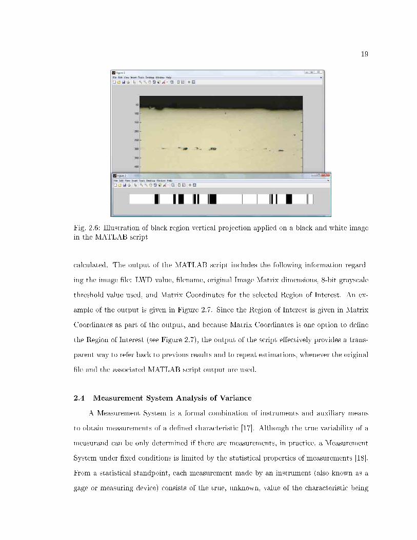
Following black and white binarization, each black pixel in black and white representa-
tion of the Region of Interest is projected across the vertical direction, as shown in Figure
2.6. The aim of this image processing task is to consider the worst case scenario of maximum
unbonded (black) pixels per row across the Region of Interest. Black pixel projection also
simpli�es further analysis by making all rows in the resulting image identical.
In MATLAB, color values for black and white colors in an Image Matrix are zeroes and
ones respectively, thus providing a means to perform mathematical operations on black and
white images. For this particular case, the color values representing black and white colored
areas will prove useful as they are associated to unbonded and bonded areas, respectively.
For instance, once black pixels are projected vertically, all pixel values in the �rst row
(comprising color values of zeroes and ones) are added up, e�ectively calculating the number
of white pixels in the �rst row. When the total sum of the �rst row of pixels is divided by the
number of pixels in the �rst row and multiplied by 100, an estimate of the LWD is obtained,
as stated in Equation (2.1).
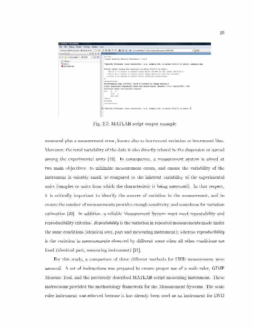
The output of the MATLAB script is printed after an estimate of the LWD has been
19
Fig. 2.6: Illustration of black region vertical projection applied on a black and white imagein the MATLAB script
calculated. The output of the MATLAB script includes the following information regard-
ing the image �le: LWD value, �lename, original Image Matrix dimensions, 8-bit grayscale
threshold value used, and Matrix Coordinates for the selected Region of Interest. An ex-
ample of the output is given in Figure 2.7. Since the Region of Interest is given in Matrix
Coordinates as part of the output, and because Matrix Coordinates is one option to de�ne
the Region of Interest (see Figure 2.7), the output of the script e�ectively provides a trans-
parent way to refer back to previous results and to repeat estimations, whenever the original
�le and the associated MATLAB script output are used.
2.4 Measurement System Analysis of Variance
A Measurement System is a formal combination of instruments and auxiliary means
to obtain measurements of a de�ned characteristic [17]. Although the true variability of a
measurand can be only determined if there are measurements, in practice, a Measurement
System under �xed conditions is limited by the statistical properties of measurements [18].
From a statistical standpoint, each measurement made by an instrument (also known as a
gage or measuring device) consists of the true, unknown, value of the characteristic being
20
Fig. 2.7: MATLAB script output example
measured plus a measurement error, known also as instrument variation or instrument bias.
Moreover, the total variability of the data is also directly related to the dispersion or spread
among the experimental units [19]. In consequence, a measurement system is aimed at
two main objectives: to minimize measurement errors, and ensure the variability of the
instrument is suitably small, as compared to the inherent variability of the experimental
units (samples or units from which the characteristic is being measured). In that respect,
it is critically important to identify the sources of variation in the measurement, and to
ensure the number of measurements provides enough sensitivity, and soundness for variation
estimation [20]. In addition, a reliable Measurement System must meet repeatability and
reproducibility criterias. Repeatability is the variation in repeated measurements made under
the same conditions (identical user, part and measuring instrument); whereas reproducibility
is the variation in measurements observed by di�erent users when all other conditions are
�xed (identical part, measuring instrument) [21].
For this study, a comparison of three di�erent methods for LWD measurement were
assessed. A set of instructions was prepared to ensure proper use of a scale ruler, GIMP
Measure Tool, and the previously described MATLAB script measuring instrument. These
instructions provided the methodology framework for the Measurement Systems. The scale
ruler instrument was selected because it has already been used as an instrument for LWD

21
assessment in UC studies, e.g. [7, 11]. Furthermore, the GIMP Measure Tool is a software-
based point-to-point distance tool that provides a free and easy-to-use alternative to manual
measurements using scale rulers.
Instruction sets serve as a guide for the proper use of the selected LWD instruments, help
users to avoid systematic errors, and take into account some particular features of each LWD
measuring device. For instance, a �xed scale was required for consistent measurements using
the scale ruler, whereas pixel units were employed with the GIMP Measure Tool in order
to improve resolution and allow zooming. Complete instruction sets used for scale ruler,
GIMP Measure Tool, and MATLAB script instruments are contained in the Addendum of
this work.
For the purposes of a Measurement System Analysis of Variance, three di�erent LWD
Measurement Systems were evaluated in this study:
� Manual on screen measurements with a scale ruler (herein and after Ruler).
� Measurements using GIMP software's Measure Tool (herein and after GIMP).
� Measurements using the Visual Clicks option of the MATLAB script (herein and after
MATLABsc).
Considering populations of cross section single-interface micrographs for all possible combi-
nations of UC parameters, a balanced experiment was performed comparing Ruler, GIMP
and MATLABsc measurement systems. Four random single-interface samples, shown in
Figure 2.8, were selected and given to ten users for LWD measurements. Each user took
three LWD measurements on each sample, as independent trials, using three di�erent gages
(measurement systems). Using statistical terminology, each con�guration of one factor is
called a factor level. In this manner, by multiplying the number of all factor levels present,
4× 10× 3× 3 = 360 observations were recorded. All treatments (factor level combinations
in the experiment) have the same number of experimental units (items for observations).
The ANOVA model for the data follows a linear combination of mixed e�ects (model
with �xed and random factors) given by:
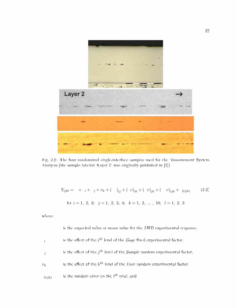
Yijkl = µ + �i + �j + υk + (��)ij + (�υ)ik + (�υ)jk + (��υ)ijk + �l(ijk)
i = 1, 2, 3; j = 1, 2, 3, 4; k = 1, 2, ..., 10; l = 1, 2, 3
µ
�i ith
�j jth
υk kth
�l(ijk) lth

23
Yijkl is the response value, namely LWD, for the lth trial, reported by the kth User,
on the jth Sample, and the ithGage.
All other terms denote interactions of respective factor levels. Other ANOVA model as-
sumptions made are:
σj are Independent and Identically-Distributed Random Variables, following a nor-
mal distribution with mean zero and variance σ2s ,
υk are Independent and Identically-Distributed Random Variables, following a nor-
mal distribution with mean zero and variance σ2u ,
(γσ)ij are Independent and Identically-Distributed Random Variables, following a nor-
mal distribution with mean zero and variance σ2a ,
(γυ)ik are Independent and Identically-Distributed Random Variables, following a nor-
mal distribution with mean zero and variance σ2b ,
(συ)jk are Independent and Identically-Distributed Random Variables, following a nor-
mal distribution with mean zero and variance σ2c , and
(γσυ)ijk are Independent and Identically-Distributed Random Variables, following a nor-
mal distribution with mean zero and variance σ2d .
In that sense, Identically-Distributed Random Variables (also noted as i.i.d) states that each
random variable has the same probability distribution, and all random variables are mutually
statistically independent (the occurrence of one event does not a�ect the probability of the
other possible outcomes to occur).
The Null Hypothesis (H0) and Alternative Hypothesis (HA) are, respectively:
H0 : γ1 = γ2 = γ3 = 0 (2.3)
HA : At least one γi 6= 0 (2.4)

24
Table 2.1: Factorial experiment Factors and Levels
Factors Levels
Gage (Measuring System) Ruler GIMP MATLABsc
User User1 User2 User3 ... User10
Sample Sample1 Sample2 Sample3 Sample4
Regarding the ANOVA model used, all factors are considered crossed with respect to all
the others, and Type 3 tests for �xed e�ects are performed for the Gage factor. In addition,
the following are some important characteristics of the ANOVA model design:
� Univariate (There is only one response or dependent variable).
� Three way factorial (that is, all combinations of User, Gage, and Sample occur in the
design).
Table 2.1 shows the experimental factors and levels for the Measuring System ANOVA:
The ANOVA was carried out using SAS� statistical software. In total, 360 observations
were initially considered, comprising three replicates (trials) of each treatment, and a critical
probability value of 0.05 was used. However, it was clear in the preliminary results that some
assumptions for the analysis were not met, and consequently, a straight ANOVA could not
be performed. The main problems encountered were the presence of heteroscedasticity and
outliers (points that depart from the overall data trend) in the data. Heteroscedasticity
means that the variance of the dependent variable (LWD measurement, in this case) varies
across data (between factor levels, in this case). For instance, the graph of Residuals against
Explanatory Factors in Figure 2.9 provided �rst hand evidence of signi�cant di�erence in
spreads (the convention in statistics is that it should not be greater than or equal to �ve
times) between the Gage factor level with the least variability (MATLABsc) and the Gage
factor level with the most variability (Ruler), where the spread is illustrated by the vertical
chain of symbols shown in the graph. It is worth noting that, in a statistical context, the
residual is the deviation of an observation from the estimated true function value, therefore,
it is an estimator of the statistical (random) error [22]. In turn, the presence of signi�cant
heteroscedasticity poses a problem because the ANOVA model is based upon, among other

25
Fig. 2.9: Residuals versus Explanatory Factors before addressing heteroscedasticity
statistical considerations, an assumption of equal variance across the data for the response
variable (homoscedasticity). As a consequence, no conclusions could be made from these
preliminary results.
It was decided to perform an ANOVA taking into account large di�erences in Gage
factor levels (Ruler, GIMP, and MATLABsc) variability. This decision was based upon
clear experimental evidence that there were signi�cant di�erences in the spread (variability)
among the levels of the Gage factor (Figure 2.10). In addition, Figure 2.9 shows that
heteroscedasticity is particularly pronounced in the Residuals versus Gage plot, suggesting
this factor is the most heteroscedastic of all.
A new ANOVA was performed by including the statement repeated / group=gage in
the PROC MIXED SAS� script, so as to include the existence of large di�erences in Gage
levels variances into the analysis. The actual PROC MIXED procedure used to carry out
the �nal ANOVA is shown below:
title3 " Using PROC MIXED with the REML Estimation Method";

26
Fig. 2.10: Box plots of the initial data showing high di�erences in Gage level variances
proc mixed data=no_trans covtest cl;
class user gage sample; model _data = gage / ddfm=satterthwaite outp = residuals;
random sample|user gage*sample gage*user gage*sample*user; repeated / group=gage;
lsmeans gage / pdiff=all adjust = Tukey; run;
These lines of code instructed SAS� statistical software to perform an ANOVA considering
the signi�cant di�erences in Gage levels spreads, while maintainig all other previous condi-
tions, and using the residual maximum likelihood (REML) approach to estimate components
of variance.
In addition, some data cleaning and outliers removal was performed, resulting in a total
of 34 neglected observations. These observations were removed because they comprised ex-
treme outliers in Residuals versus Normal Percentiles plots for each Gage factor level. The
presence of these extreme outliers diagnostic hinders the validity of any futher Analysis of
Variance, because one of the ANOVA premises is that residuals are normally distributed
according to the mathematical theory of errors [22]. As shown in Figure 2.11, the outliers
do not re�ect the data general line of orientation. After thoughtful considerations, it was
decided to withdraw these outliers from the �nal data set. The �nal ANOVA included large

27
variances di�erences in Gage levels into the analysis and conprises data of only 326 �nal
observations. However, it is worth mention that preliminary straight ANOVA results includ-
ing outliers (all available data) drew equivalent conclusions to the �nal ANOVA inferences.
Hereinafter, results of the �nal ANOVA performed are presented.
The Residuals versus Explanatory Factors plots of the �nal ANOVA are shown in
Figure 2.12 and include additional evidence of Gage factor heteroscedasticity. However,
this heteroscedastic Gage factor was expected and the �nal ANOVA has been performed
taking into account those signi�cant di�erences in Gage factor level spreads. Furthermore,
the Residuals versus Predicted Values plot for the �nal data (without outliers) in Figure
3.12 does not show signi�cant evidence of heteroscedasticity since there is not any evident
gradient pattern (e.g. a megaphone shape) in the Residuals versus Predicted values plot.
In sum, Residuals versus Explanatory Factors plots provide no reason to invalidate �nal
ANOVA results.
Diagnostics con�rm that the residuals normality assumption is quite reasonable after
performing statistical diagnostics for each level of Gage (Residuals versus Normal Percentiles
plots for each level of the Gage factor all show a fairly straight line), as shown in Figure 2.14.
In the case of the MATLABsc level of the Gage factor, there is concentration of points near
the zero residual value that is of some concern. However, in light of the evidence provided
by the MATLABsc histogram (Figure 2.15) and MATLABsc Boxplots and Stem-Leaf plots
(Figure 2.16), MATLABsc data was deemed approximately normal, since it resembles a
bell-shaped curve with a low standard deviation. Similarly, histograms for the rest of Gage
factor levels suggest a reasonable normal distribution �t, as shown in Figure 2.15. Moreover,
Boxplots and Stem-Leaf plots for Ruler and GIMP (Figure 2.16) both support reasonable
normality based upon graphical correspondence with the bell-shaped distribution of values.
As stated in the ANOVA model, the Null Hypothesis (H0) postulated in Equation
2.3 that there was no e�ect due to the Gage factor on the LWD value, meaning that the
mean, variance, and shape of all Gage factor level samples' distributions would be identical.
In that respect, a p-value is calculated in order to accept or reject the Null Hypothesis.

28
Fig.2.11:Rem
oved
outliersas
show
nin
ResidualsvsNormalPercentilesplotsforeach
Gagefactor
level

29
Fig. 2.12: Residuals versus Explanatory Factors plots in �nal ANOVA
The p-value is the probability of obtaining results at least as extreme as the one that was
actually observed, assuming that the Null Hypothesis is true. In our case, since the critical
probability value used in this study is 0.05, it means that the Null Hypothesis would be
rejected if a p-value equal or less than 0.05 (5% of expected likelihood) is obtained. A Type
3 F-test is performed in the Type 3 Tests of Fixed E�ects table (Figure 2.17) because the test
statistic associated to the p-value has an F-probability distribution [23], and SAS� utilizes
Type 3 F-tests to assess di�erences between Least Squares Means (LSM) for mixed e�ects,
instead of using di�erences between the arithmetic treatment means (Type 1 F-test) [24].
In this context, it is worth mentioning that LSM are obtained by performing a regression
analysis using the ANOVA model stated in Equation (3.2). As for the ANOVA results,
Figure 2.17 shows that a statistically signi�cant p-value of 0.0101 for the Gage factor was
obtained as a result of a Type 3 F-test (the p-value obtained is equal or less than the selected
critical probability value of 0.05). Consequently, based upon the present statistical study,
the condition for the Null Hypothesis to be true is not met, and it is concluded that Gage

30
Fig. 2.13: Residuals versus Predicted values plot in �nal ANOVA
a�ects LWD measurements. In fact, this Type 3 F-test result provides statistical evidence of
the signi�cant e�ect of the Gage factor on the LWD response, and prompts for a comparison
between the three Gage factor level means. The Least Squares Means table shown in Figure
2.17 also reveals that all three Gage factor level means are statistically signi�cant for LWD
measurements (the p-values shown in the Pr > |t| column of the LSM table are all equal or
less than the 0.05 probability critical value). Furthermore, the Di�erence of Least Squares
Means table in Figure 2.17 presents statistical evaluations on pairwise combinations of Gage
factor levels means. In this context, the di�erence between Ruler and MATLABsc LWD
means were not signi�cant (evidenced by the fact the 1.0000 p-value obtained is greater
than the selected critical probability value of 0.05). In conclusion, the Di�erence of Least
Squares Means table shows that, based upon the present statistical evidence, measurements
taken with MATLABsc and Ruler gages have the same mean, although this does not hold
true for any other pair of measuring systems (Ruler-GIMP and GIMP-MATLABsc).
2.5 Discussion
Based upon Measurement System ANOVA results shown in the LSM table (Figure
2.17), the e�ects of all measurement systems (Gage factor levels) evaluated in this study are
signi�cant in a�ecting LWD measurements on micrographs. Therefore, the selection between
Ruler, GIMP, and MATLABsc measurement systems matters in determining LWD values
on ultrasonically consolidated samples. Moreover, MATLABsc data exhibits the minimum

31
Fig.2.14:ResidualsvsNormalPercentilesplotforeach
Gagefactor
levelin
�nalANOVA

32
Fig.2.15:Histogram
foreach
Gagefactor
levelin
�nalANOVA


34
Fig. 2.17: Type 3 �xed e�ects test and Least Squares Means for Gage factor in �nal ANOVA
face speci�cation (in sample micrographs with multiple layers) and provides computational
simpli�cation for further image processing. However, the interface shown in the Image File
input (Figure 2.1) must be horizontally oriented, and it is crucial to de�ne the Region of
Interest as close as possible to the interface in order to perform a correct analysis. In this
respect, MATLAB has limited dynamic zoom capabilities to facilitate the selection of the
Region of Interest using the Visual Clicks option. Speci�cally, the zoom in/out option can
only be used in the MATLAB script routine when the initial image is initially shown on
screen (Figure 2.1), and the zoom magni�cation level cannot be adjusted afterwards. For
this reason, it is also important to set an adequate magni�cation level for sample microscopy.
For picture-wide interfaces, the recommended magni�cation level range for de�ning the ROI
to obtain a LWD estimate using the MATLAB script is 50-100X. Based on several tests per-
formed, some defects could not be clearly seen inside the MATLAB �gure window with a mi-
croscopy magni�cation level lower than 50X, without zoom. At the other end, picture-wide
interfaces do not have enough interface length for proper analysis when using microscopy
magni�cation levels above 100X. For ROI de�nitions that are not picture-wide, the zoom
option available in the MATLAB script routine can be used with magni�cation levels above
100X and below 50X, and the practical minimum/maximum magni�cation for microscopy
35
will depend upon the speci�c application. The MATLAB script procedure is designed to
work with only one micrograph. Multiple or combined image analysis using the MATLAB
script is only indirectly possible at this development point, by stitching together multiple
side-by-side micrographs to make a single micrograph of a horizontally oriented contiguous
interface, for further analysis. On the other hand, it is worth mention that stitching to-
gether micrographs may induce artifacts in the image as opposed to taking individual LWD
measurements on each interface, tabulating them in a spreadsheet and averaging.
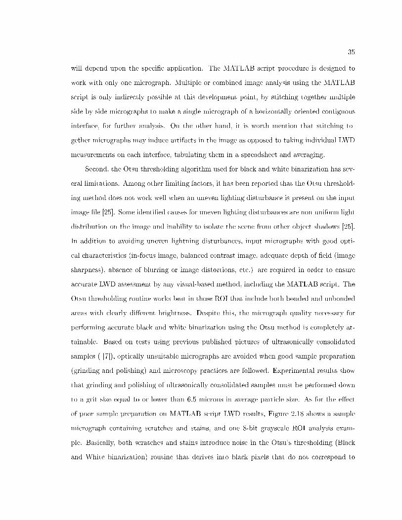
Second, the Otsu thresholding algorithm used for black and white binarization has sev-
eral limitations. Among other limiting factors, it has been reported that the Otsu threshold-
ing method does not work well when an uneven lighting disturbance is present on the input
image �le [25]. Some identi�ed causes for uneven lighting disturbances are non-uniform light
distribution on the image and inability to isolate the scene from other object shadows [25].
In addition to avoiding uneven lightning disturbances, input micrographs with good opti-
cal characteristics (in-focus image, balanced contrast image, adequate depth of �eld (image
sharpness), absence of blurring or image distortions, etc.) are required in order to ensure
accurate LWD assessment by any visual-based method, including the MATLAB script. The
Otsu thresholding routine works best in those ROI that include both bonded and unbonded
areas with clearly di�erent brightness. Despite this, the micrograph quality necessary for
performing accurate black and white binarization using the Otsu method is completely at-
tainable. Based on tests using previous published pictures of ultrasonically consolidated
samples ( [7]), optically unsuitable micrographs are avoided when good sample preparation
(grinding and polishing) and microscopy practices are followed. Experimental results show
that grinding and polishing of ultrasonically consolidated samples must be performed down
to a grit size equal to or lower than 6.5 microns in average particle size. As for the e�ect
of poor sample preparation on MATLAB script LWD results, Figure 2.18 shows a sample
micrograph containing scratches and stains, and one 8-bit grayscale ROI analysis exam-
ple. Basically, both scratches and stains introduce noise in the Otsu's thresholding (Black
and White binarization) routine that derives into black pixels that do not correspond to

36
unbonded areas, and leads to inaccurate LWD results. The sample must be in not-etched
condition because etching creates small cavities that appear as dark areas in micrographs,
causing a similar e�ect to the ROI analysis as the one caused by the stains and scratches.
Moreover, good sample preparation (grinding and polishing) is critical due to the brightness
criteria used in the MATLAB script procedure to make the distinction between bonded and
unbonded regions in the ROI. In general, the MATLAB script does not automatically dif-
ferentiate between unbonded regions, scratches, stains and etching marks in the Region of
Interest. In fact, the MATLAB script gives a conservative LWD estimate for the Region of
Interest and any black pixel out of the interlayer interface will result in a LWD assessment
bias. For instance, as is shown in Figure 2.18, it only takes one black pixel in a column of
the ROI Image Matrix to render the entire column as unbonded area. Thus it is important
that users of the MATLAB script look at the Otsu thresholding results to make sure there
are no stray black pixels outside the interface region that will a�ect the LWD measurement,
before black pixels are extended vertically across the image.
That being said, it is worth a mention that the MATLAB script can be used to perform
LWD measurements on micrographs including multiple interfaces, although in its current
implementation, the procedure can only process one interface per run.
The MATLABsc measurement system is also e�cient in assessing LWD. For compara-
tive purposes, Table 2.2 shows the average time per user per sample to take LWD measure-
ments (in seconds) using each measuring system of this study. Overall, the amount of time
to take measurements using the MATLAB script is 46.36% (65.25−3565.25 ) less than that of the
Ruler and 57.70% (82.75−3582.75 ) less than that of the GIMP.
2.6 Summary and Conclusion
The experimental results presented show that the MATLAB script can e�ectively esti-
mate LWD on cross section micrographs. Although there are some limitations for the Image
Processing approach used in the MATLAB script routine, this LWD instrument provides
the highest resolution of all measuring devices presented in this work.
Moreover, the MATLABsc measuring system shows small spread or variation in the

37
Fig.2.18:Bad
specimen
preparationexam
ple
38
Table 2.2: Measuring systems time comparison
Average time (s)
Specimen Ruler GIMP MATLABsc
1 57 63 26
2 73 97 31
3 50 55 45
4 81 116 38
Grand average time: 65.25 82.75 35
measurements, and a veri�able methodology to assess LWD in cross section micrographs
that is suitable for standardization. In fact, when considering the MATLABsc measuring
system spread as a unit, Figure 2.10 shows that the spreads of GIMP and Ruler measuring
systems are at least 7.4 and 8.7, respectively.
In addition, experimental results show that Ruler and MATLAB instruments have
statistically similar measurement means, and thus the MATLAB script can be used to
compare results against past Ruler measurements.
2.7 Future Work
In order to improve upon the usability of the and robustness of the MATLAB script,
recommended future work includes the development of a method for e�cient identi�cation
of sample defects (voids, delamination, inclusions) for better LWD assessment, and the
incorporation of an option for processing multiple interfaces in one micrograph in order to
provide an average LWD estimate.
The latest version of the MATLAB script is available for free under the terms contained
in the lwd.m script �le and can be downloaded from:
https://sites.google.com/site/lwdmatlabsc/
Additional work needs to be done in order to present a complete LWD measurement stan-
dard. This includes:
� Specifying the minimum requirements for the optical system used to acquire ultrason-
ically consolidated sample micrographs.

39
� De�ning a standard for weldment preparation in terms of preparation times, speci�c
preparation materials/equipment, and preparation methods in tandem with the ultra-
sonically consolidated material used and the level of quality desired.
Addendum
Instructions for Ruler, GIMP and MATLAB script gages for measuring LWD.
� Ruler Instructions:
1. Open the GIMP program.
2. On the GIMP Menu bar, select `File->Open...', select the image �le of interest and
press `Open'.
3. Maximize the window containing the image �le.
4. Using the 1:200 scale of the metric scale ruler and having the image displayed, mea-
sure total horizontal interface length on the screen with the ruler, at current zoom
magni�cation level. Record this measurement.
5. Using the 1:200 scale of the metric scale ruler and having the image displayed, measure
the horizontal length of each black pixel region in the interface with the ruler, keeping
the same zoom magni�cation level used in the previous step. Perform all measurements
on screen and record each length value.
6. Add up the lenghts of each individual black pixel regions obtained in the previous step
to get the Unbonded interface length.
7. Using results from steps 3 and 5, calculate LWD by using the formula:
%LWD = Total interface length−Unbonded interface lengthTotal interface length × 100
8. Repeat steps 2 through 6 with all given sample images and save all LWD results.
� GIMP Measure Tool Instructions:

40
1. Open the GIMP program.
2. On the GIMP Menu bar, select `File->Open...', select the image �le of interest and
press `Open'.
3. Having the image displayed on screen, go to the GIMP program Menu Bar, and select
`Tools->Measure'.
4. Select pixels as length units in the Status Bar of the GIMP window where the image
is displayed in.
5. Measure total horizontal interface length in the interface by clicking and dragging the
mouse cursor, and record this measurement. You may use Ctrl+Mouse Wheel Scroll
to zoom in or out with respect to the original view.
6. Measure the horizontal length of each black pixel region in the interface by clicking
and dragging the mouse cursor, and record each length value in pixels. You may use
Ctrl+Mouse Wheel Scroll to zoom in or out with respect to the original view.
7. Add up the lenghts of each individual black pixel regions obtained in the previous step
to get the Unbonded interface length.
8. Using results from steps 5 and 7, calculate LWD by using the formula:
%LWD = Total interface length−Unbonded interface lengthTotal interface length × 100
9. Repeat steps 2 through 7 for each one of the sample images. Save all LWD results.
10. Close GIMP program.
� MATLAB Script Visual Clicks Instructions:
1. Start MATLAB program. Place `lwd.m' MATLAB script �le and all image �les of
interest in the MATLAB working directory.
2. Enter `lwd' (without quotes) at MATLAB command window prompt to run the MAT-
LAB script for LWD measurements.

41
3. Follow on-screen instructions for image �le input.
4. When the sample image is shown in a MATLAB Figure window, con�rm image �le
selection by pressing Enter, or cancel execution by pressing Ctrl+c while the MATLAB
window is active. You may use Ctrl+Mouse Wheel Scroll to zoom in or out with respect
to the original view at this step. If you cancel the MATLAB script execution, repeat
steps 2 and 3.
5. Select a region for the analysis using the mouse clicks option. Two separate clicks
specify two diagonally opposite corners of the rectangle that enclose the interface.
This click-de�ned rectangle should be the smallest section of the image that contains
the interface to be analyzed. If necessary, you may click outside the image and the
selection will be adjusted to match the image borders automatically. Do not select the
whole image as your rectangular region.
6. Press enter three times for grayscale images, or four times for color images as it applies.
The LWD estimate is given as part of the output in the MATLAB command window,
between discontinuous lines (- - -). Record this LWD measurement.
7. Repeat steps 2 through 6 for each one of the sample images. If an error is encountered,
re-run the script again (repeat steps 2 through 6). Save all LWD results.
8. Exit the MATLAB script routine by pressing Ctrl+c while the MATLAB window is
active.
9. Close MATLAB program.
42
Chapter 3
Experimental Determination of Optimum Parameters for
Stainless Steel 316L Annealed Ultrasonic Consolidation1
3.1 Abstract
Ultrasonic Consolidation of Stainless Steel foils is being investigated for potential struc-
tural applications. In this study, parameter optimization for Ultrasonic Consolidation of
Stainless Steel 316L annealed is assessed by evaluating experimental factors of Oscillation
Amplitude, Welding Speed, and Normal Force at 478 K (400 °F). A series of experiments
were performed to explore the e�ect of these factors on the Linear Welding Density of utra-
sonically consolidated samples, determine the statistical signi�cance of these factors, and
identify the combination of UC process parameters that maximizes Linear Welding Density.
3.2 Introduction
Ultrasonic Consolidation (UC) is an additive manufacturing process whereby layers of
metal foils can be joined with a metallurgical bond by means of acoustic energy and shaped
using CNC machining. The UC process has the advantage of creating metal structures
without high temperatures [6]. Indeed, although localized frictional heating is involved in
the UC process, the mechanism for UC is not melting [6], and thus negligible shrinkage
and thermal stresses result during part building [5]. In turn, ultrasonically consolidated
parts have virtually no thermal degradation in material properties. Although there are
some limitations regarding how high ultrasonically consolidated parts can be made [26],
1Coathored by R. Gonzalez, B. Stucker. This chapter is a paper that has been submitted for publication
in the Rapid Prototyping Journal.
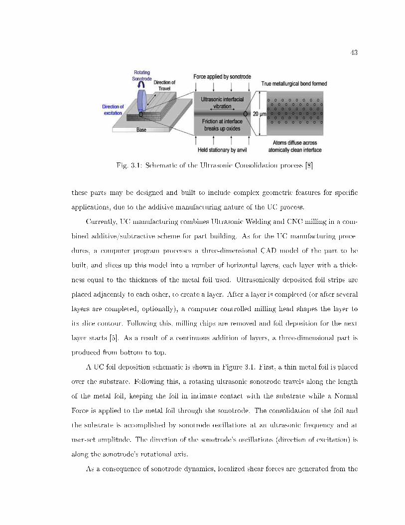
43
Fig. 3.1: Schematic of the Ultrasonic Consolidation process [8]
these parts may be designed and built to include complex geometric features for speci�c
applications, due to the additive manufacturing nature of the UC process.
Currently, UC manufacturing combines Ultrasonic Welding and CNC milling in a com-
bined additive/subtractive scheme for part building. As for the UC manufacturing proce-
dures, a computer program processes a three-dimensional CAD model of the part to be
built, and slices up this model into a number of horizontal layers, each layer with a thick-
ness equal to the thickness of the metal foil used. Ultrasonically deposited foil strips are
placed adjacently to each other, to create a layer. After a layer is completed (or after several
layers are completed, optionally), a computer controlled milling head shapes the layer to
its slice contour. Following this, milling chips are removed and foil deposition for the next
layer starts [5]. As a result of a continuous addition of layers, a three-dimensional part is
produced from bottom to top.
A UC foil deposition schematic is shown in Figure 3.1. First, a thin metal foil is placed
over the substrate. Following this, a rotating ultrasonic sonotrode travels along the length
of the metal foil, keeping the foil in intimate contact with the substrate while a Normal
Force is applied to the metal foil through the sonotrode. The consolidation of the foil and
the substrate is accomplished by sonotrode oscillations at an ultrasonic frequency and at
user-set amplitude. The direction of the sonotrode's oscillations (direction of excitation) is
along the sonotrode's rotational axis.
As a consequence of sonotrode dynamics, localized shear forces are generated from the

44
combination of sonotrode pressure and oscillation, inducing interfacial stresses between the
two mating surfaces and elastic-plastic deformation of surface asperities [6]. Furthermore,
asperities deformations break up the oxide �lm, establishing a metallurgical bond between
the foil and the substrate due to relatively clean metal-to-metal surface contact [5]. On a
lower scale, atomic di�usion may also aid in the bonding process because local temperatures
at the interface and the surrounding a�ected region (about 20 µm) can reach up to 50% of the
melting point of the material being deposited [6], but only for a very brief time. Although still
being researched, there is evidence that ultrasonic welding mechanisms for bond formation
involve: (1) removal of surface oxide layers, (2) plastic deformation at the interface, and
(3) to a lesser extent, di�usion of metal atoms across the interface. Nonetheless, plastic
deformation is considered the most important characteristic in enabling surface oxide layer
removal and di�usion mechanisms [7]. All three mechanisms aid in metallurgical bonding
across the interface.
There are four general control parameters for welding within a UC system: Amplitude
of Oscillation, Contact Pressure Distribution (Normal Force between the horn and foil),
Welding Speed along the direction of travel, and Temperature of the substrate. The �rst
three parameters depend upon sonotrode interaction with the part being built. In contrast,
Temperature depends on the heat applied directly to the substrate from the base plate, with
Temperature values from room temperature up to hundreds of kelvin degrees (e.g. typical
platform's limitation is 478 K (400 °F)).
Linear Welding Density (LWD) is the proportion of bonded area to total area within
the weld interface [9]. The selection of LWD as a quality measure is better understood
considering that ultrasonically consolidated parts typically show unbounded regions (defects,
physical discontinuities) along the layer interfaces. Indeed, the assessment of the bonded
region proportion given in a LWD measurement is also important as a quality attribute
for porosity in ultrasonically consolidated parts [11]. The relevance of understanding what
factors in�uence LWD has already been observed in a previous study of UC parts [7]. As a
matter of fact, LWD strongly a�ects mechanical properties in the direction normal to the foils
45
for an ultrasonically consolidated part, and the mechanical behavior of a UC made structure
under load-bearing stresses [7]. In consequence, properties like speci�c weight and Poisson's
ratio of ultrasonically consolidated parts are a�ected by LWD. In the same manner, quality
charateristics based on ultrasonically consolidated part porosity (e.g. insulating enclosures)
are utterly dependent upon the level of LWD present between metal foils.
For the purposes of this study, LWD will be determined based upon metallography of
weld interfaces sectioned along the width of the foil. The samples will be mounted, polished
to a smooth �nish and cleaned in isopropyl alcohol. LWD will be assessed from micrograph
images of samples taken from weld cross-sections, based upon the following equation:
%LWD =Bonded interface length
Total interface length× 100 (3.1)
Regarding optimum parameters for UC, it is worth mentioning that optimality is not
absolute under general conditions. The magnitude of interfacial stresses at the mating sur-
faces during the UC process depends on current frictional conditions at the sonotrode/foil
and substrate/foil interfaces [8,27�29]. Furthermore, sonotrode geometry, material, and sur-
face conditions in�uence optimum parameter values for UC [11]. Consequently, UC optimum
process parameters can vary with sonotrode wear over time, di�erent foil material/thickness
and for di�erent UC systems. In general, a signi�cant change in frictional conditions at
the sonotrode/foil or substrate/foil interfaces will a�ect optimum UC parameter values.
Therefore, it is necessary to understand that the concept of optimality of UC parameters
is restricted to a reasonably consistent range of frictional conditions, whereas new optimum
UC process parameters must be established if these frictional conditions change signi�cantly.
Overall, the objectives of the research e�ort presented here are to (1) Determine the
optimum processing parameters for UC of Stainless Steel 316L annealed (SS316L annealed)
foils, based on the maximum Linear Welding Density criteria; and (2) Characterize the
e�ect that optimum UC parameters have on SS316L annealed ultrasonically consolidated
samples. SS316L annealed was chosen due to its commercial availability in foil form, variety
of applications and greater mechanical strength than Aluminum (Al) 3003 � the typical

46
material used in UC machines. Additionally, research on SS316L UC will allow comparison
between previous Al UC studies and this investigation. Even though some researchers
have recommended a joint approach for determining optimum UC parameters based on
peel testing and LWD measurements [9], the criteria used in this study is minimal part
porosity and thus maximum LWD is the benchmark used for determining the optimum UC
parameters in this work. Although Peel Strength is another parameter for characterizing
ultrasonically consolidated parts, it has been found that peel test results are notoriously
scattered compared to LWD, and thus LWD appears to be a more stable parameter [30].
3.3 Literature Review
In previous studies, UC of 3003/6061 Al alloy structures have been investigated using
Welding Speed, Oscillation Amplitude, Temperature, and Contact Pressure as the variable
process parameters [9, 11, 13]. The evaluation of the e�ect the aforementioned parameters
had on microstructure and mechanical properties of ultrasonically consolidated parts has
been the object of active research [9, 10]. In this context, selection of appropriate process
parameters plays a key role in UC bond formation of Al 3003/6061 based on LWD micro-
scopic studies and peel-o� tests [9, 10]. Although authors have found that it is possible to
have a low peel load response and high linear weld density with Aluminum 6061 (due to
excessive strain hardening and cycling stressing of contact points at the interface) [9]; it has
been veri�ed that a high peel load response only occurs in the presence of high LWD [10].
For instance, higher Oscillation Amplitude values produced higher LWD in Al 3003/6061
and either higher weld strengths (in Al 3003) [10] or no signi�cant e�ect on weld strength
(in Al 6061) [9]. Furthermore, several research e�orts included Substrate Temperature as an
additional factor for the Al 3003 UC process, and performed a comprehensive study of the
e�ect of Substrate Temperature, Welding Speed, Oscillation Amplitude, Surface Machining
and Normal Force on Al 3003 UC [7,11]. Among other things, it was concluded that higher
Normal Force and higher Oscillation Amplitude increase LWD values up to a certain level,
beyond which LWD values decrease. Moreover, it was observed that lower Welding Speeds
(down to 12 mm/s) increase LWD, and higher temperatures produced higher LWD within
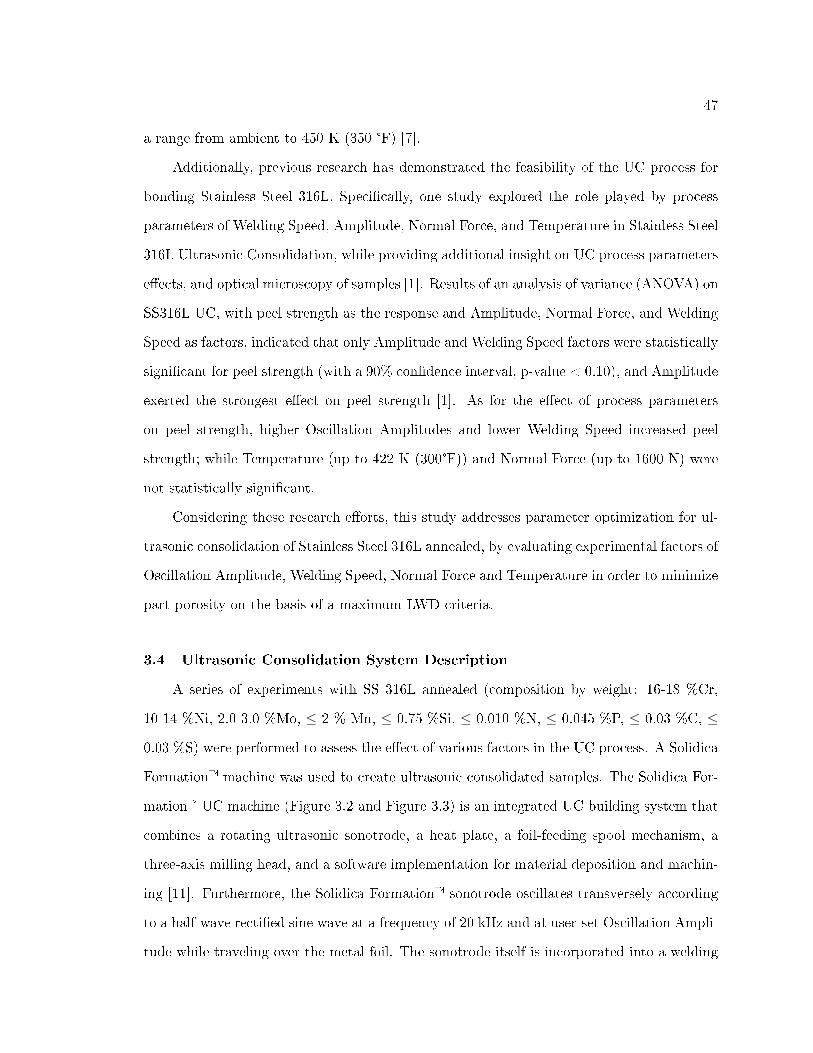
47
a range from ambient to 450 K (350 °F) [7].
Additionally, previous research has demonstrated the feasibility of the UC process for
bonding Stainless Steel 316L. Speci�cally, one study explored the role played by process
parameters of Welding Speed, Amplitude, Normal Force, and Temperature in Stainless Steel
316L Ultrasonic Consolidation, while providing additional insight on UC process parameters
e�ects, and optical microscopy of samples [1]. Results of an analysis of variance (ANOVA) on
SS316L UC, with peel strength as the response and Amplitude, Normal Force, and Welding
Speed as factors, indicated that only Amplitude and Welding Speed factors were statistically
signi�cant for peel strength (with a 90% con�dence interval, p-value < 0.10), and Amplitude
exerted the strongest e�ect on peel strength [1]. As for the e�ect of process parameters
on peel strength, higher Oscillation Amplitudes and lower Welding Speed increased peel
strength; while Temperature (up to 422 K (300°F)) and Normal Force (up to 1600 N) were
not statistically signi�cant.
Considering these research e�orts, this study addresses parameter optimization for ul-
trasonic consolidation of Stainless Steel 316L annealed, by evaluating experimental factors of
Oscillation Amplitude, Welding Speed, Normal Force and Temperature in order to minimize
part porosity on the basis of a maximum LWD criteria.
3.4 Ultrasonic Consolidation System Description
A series of experiments with SS 316L annealed (composition by weight: 16-18 %Cr,
10-14 %Ni, 2.0-3.0 %Mo, ≤ 2 % Mn, ≤ 0.75 %Si, ≤ 0.010 %N, ≤ 0.045 %P, ≤ 0.03 %C, ≤
0.03 %S) were performed to assess the e�ect of various factors in the UC process. A Solidica
Formation� machine was used to create ultrasonic consolidated samples. The Solidica For-
mation� UC machine (Figure 3.2 and Figure 3.3) is an integrated UC building system that
combines a rotating ultrasonic sonotrode, a heat plate, a foil-feeding spool mechanism, a
three-axis milling head, and a software implementation for material deposition and machin-
ing [11]. Furthermore, the Solidica Formation� sonotrode oscillates transversely according
to a half-wave recti�ed sine wave at a frequency of 20 kHz and at user-set Oscillation Ampli-
tude while traveling over the metal foil. The sonotrode itself is incorporated into a welding

48
head and its position is controlled by numerical control. The maximum build size of the
Solidica Formation� machine is 609.6 mm × 914.4 mm × 203.2 mm (24 in × 36 in × 8
in), and the CNC contour milling head has a tolerance of 0.05 mm (0.002 in) [12]. The
sonotrode has a 146.75 mm nominal diameter. Regarding process parameter setting limits,
the Solidica Formation� machine is constrained to a nominal force less than or equal to
1800 N, nominal amplitudes between 6 µm and 27 µm, welding speeds up to 84.7 mm/s (200
ipm), and nominal temperatures ranging from ambient to 478 K (400 °F).
Using the Solidica Formation� system, part fabrication is performed on a �rmly bolted
Al 3003 H14 (composition by weight: 0.050-0.20 %Cu, ≤ 0.70 %Fe, 1.0-1.50 %Mn, ≤ 0.60
%Si, ≤ 0.10 %Zn) base plate mounted on a heat plate. Also, the heat plate maintains
the substrate at a user-set Temperature, between ambient and 478 K (400°F). A graphical
description of the Al 3003 H14 base plate (dimensions: 355 mm × 355 mm × 12 mm) along
with the plate/part �xture is presented in Figure 3.4.
A 146.75 mm nominal diameter Titanium sonotrode was employed for UC depositions.
Sonotrode roughness was measured using a Mitutoyo Surftest SV-602 stylus pro�lometer,
at three evenly spaced angular locations (0 rad (0°), 2π3 rad (120°), 4π
3 rad (240°)). The
Arithmetic Average of Absolute Values (Ra) was calculated in the sonotrode direction of
excitation and around the sonotrode midplane circumference (a one inch long arc centered
at each angle location). Results for Ra calculations are presented in Table 3.1.
3.5 Experimental Work
Table 3.1: Sonotrode surface roughmess measurements
Sonotrode Angular Location
Measurement Type 0 rad (0°) 2π3 rad (120°) 4π
3 rad (240°)
Ra (µm) in the direction of oscillations 6.06 4.74 4.81
Ra (µm) around the circumference 5.01 3.96 6.59

49
Fig. 3.2: Solidica Formation� machine (as shown in [11])
Fig. 3.3: Close-up view of the Welding head, showing the sonotrode from below (as shownin [11])
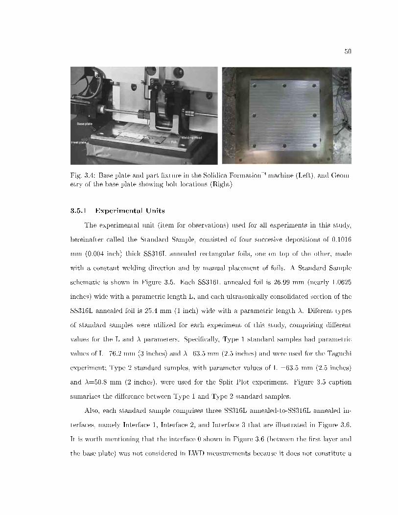
50
Fig. 3.4: Base plate and part �xture in the Solidica Formation� machine (Left), and Geom-etry of the base plate showing bolt locations (Right)
3.5.1 Experimental Units
The experimental unit (item for observations) used for all experiments in this study,
hereinafter called the Standard Sample, consisted of four succesive depositions of 0.1016
mm (0.004 inch) thick SS316L annealed rectangular foils, one on top of the other, made
with a constant welding direction and by manual placement of foils. A Standard Sample
schematic is shown in Figure 3.5. Each SS316L annealed foil is 26.99 mm (nearly 1.0625
inches) wide with a parametric length L, and each ultrasonically consolidated section of the
SS316L annealed foil is 25.4 mm (1 inch) wide with a parametric length λ. Diferent types
of standard samples were utilized for each experiment of this study, comprising di�erent
values for the L and λ parameters. Speci�cally, Type 1 standard samples had parametric
values of L=76.2 mm (3 inches) and λ=63.5 mm (2.5 inches) and were used for the Taguchi
experiment; Type 2 standard samples, with parameter values of L =63.5 mm (2.5 inches)
and λ=50.8 mm (2 inches), were used for the Split Plot experiment. Figure 3.5 caption
sumarizes the di�erence between Type 1 and Type 2 standard samples.
Also, each standard sample comprises three SS316L annealed-to-SS316L annealed in-
terfaces, namely Interface 1, Interface 2, and Interface 3 that are illustrated in Figure 3.6.
It is worth mentioning that the interface 0 shown in Figure 3.6 (between the �rst layer and
the base plate) was not considered in LWD measurements because it does not constitute a

51
Stainless Steel to Stainless Steel bond and, in contrast with layer depositions corresponding
to Interfaces 1, 2, and 3, there is no initial sonotrode-induced roughness on the substrate.
3.5.2 Taguchi Experiment
An exploratory Taguchi Design was used to look into the e�ect UC process parameters
or Factors (Oscillation Amplitude, Welding Speed, Normal Force and Temperature) have on
the LWD of SS316L ultrasonically consolidated samples and pinpoint working combinations
of UC parameters for SS316L annealed UC. Using statistical terminology, each evaluated
con�guration of one factor is called a factor level. The Taguchi experiment design comprised
four di�erent levels for each parameter, and this is illustrated in Table 3.2. Levels for
UC parameters for the Taguchi experiment were selected based upon Solidica Formation�
machine design limits, SS316L annealed UC feasibility tests available in the literature [1],
and the combination of UC parameters that produced maximum LWD for Al 3003 UC
reported by some researchers [7].
A special Taguchi L-16 orthogonal array, namely the L'16 (45 L-16) Taguchi orthogonal
array, was utilized to determine the e�ects of individual process parameters. The L'16 array
comprises �ve di�erent experimental factors, four levels each [31]. Since only four process
parameters are being considered for the Taguchi experiment, the �fth factor corresponding to
the �fth column of the L'16 orthogonal array was not included and the Taguchi experiment
array in Table 3.3 was obtained. Each experimental run produced one Type 1 standard
Fig. 3.5: Schematic of a SS316L annealed Standard Sample (In Type 1: L =76.2 mm (3inches), λ=63.5 mm (2.5 inches); In Type 2: L =63.5 mm (2.5 inches), λ=50.8 mm (2inches))
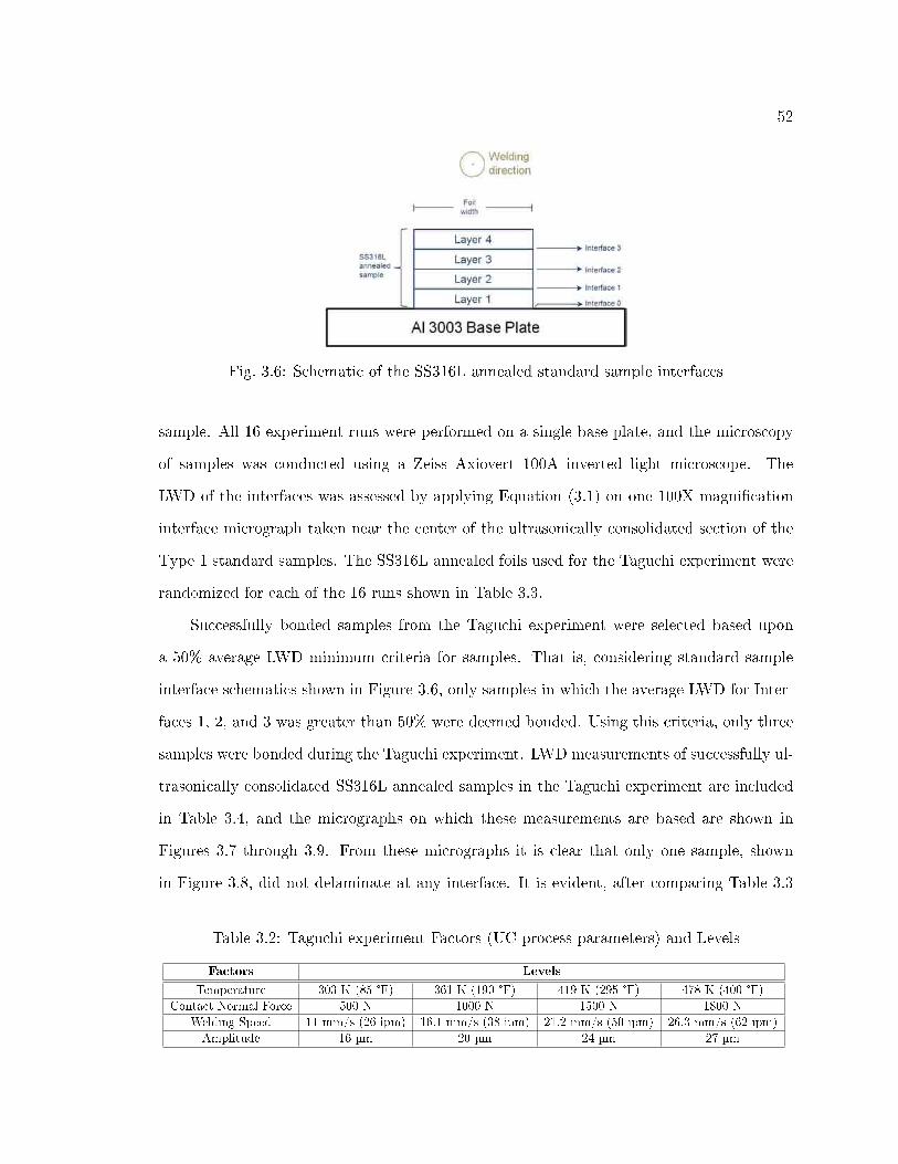
52
Fig. 3.6: Schematic of the SS316L annealed standard sample interfaces
sample. All 16 experiment runs were performed on a single base plate, and the microscopy
of samples was conducted using a Zeiss Axiovert 100A inverted light microscope. The
LWD of the interfaces was assessed by applying Equation (3.1) on one 100X magni�cation
interface micrograph taken near the center of the ultrasonically consolidated section of the
Type 1 standard samples. The SS316L annealed foils used for the Taguchi experiment were
randomized for each of the 16 runs shown in Table 3.3.
Successfully bonded samples from the Taguchi experiment were selected based upon
a 50% average LWD minimum criteria for samples. That is, considering standard sample
interface schematics shown in Figure 3.6, only samples in which the average LWD for Inter-
faces 1, 2, and 3 was greater than 50% were deemed bonded. Using this criteria, only three
samples were bonded during the Taguchi experiment. LWD measurements of successfully ul-
trasonically consolidated SS316L annealed samples in the Taguchi experiment are included
in Table 3.4, and the micrographs on which these measurements are based are shown in
Figures 3.7 through 3.9. From these micrographs it is clear that only one sample, shown
in Figure 3.8, did not delaminate at any interface. It is evident, after comparing Table 3.3
Table 3.2: Taguchi experiment Factors (UC process parameters) and Levels
Factors Levels
Temperature 303 K (85 °F) 361 K (190 °F) 419 K (295 °F) 478 K (400 °F)Contact Normal Force 500 N 1000 N 1500 N 1800 N
Welding Speed 11 mm/s (26 ipm) 16.1 mm/s (38 ipm) 21.2 mm/s (50 ipm) 26.3 mm/s (62 ipm)
Amplitude 16 µm 20 µm 24 µm 27 µm

53
Table 3.3: Taguchi L'16 experiment runs matrix
Experiment run Temperature Normal Force Welding Speed Amplitude
1 303 K (85 °F) 500 N 11 mm/s (26 ipm) 16 µm2 303 K (85 °F) 1000 N 16.1 mm/s (38 ipm) 20 µm3 303 K (85 °F) 1500 N 21.2 mm/s (50 ipm) 24 µm4 303 K (85 °F) 1800 N 26.3 mm/s (62 ipm) 27 µm5 361 K (190 °F) 500 N 16.1 mm/s (38 ipm) 24 µm6 361 K (190 °F) 1000 N 11 mm/s (26 ipm) 27 µm7 361 K (190 °F) 1500 N 26.3 mm/s (62 ipm) 16 µm8 361 K (190 °F) 1800 N 21.2 mm/s (50 ipm) 20 µm9 419 K (295 °F) 500 N 21.2 mm/s (50 ipm) 27 µm10 419 K (295 °F) 1000 N 26.3 mm/s (62 ipm) 24 µm11 419 K (295 °F) 1500 N 11 mm/s (26 ipm) 20 µm12 419 K (295 °F) 1800 N 16.1 mm/s (38 ipm) 16 µm13 478 K (400 °F) 500 N 26.3 mm/s (62 ipm) 20 µm14 478 K (400 °F) 1000 N 21.2 mm/s (50 ipm) 16 µm15 478 K (400 °F) 1500 N 16.1 mm/s (38 ipm) 27 µm16 478 K (400 °F) 1800 N 11 mm/s (26 ipm) 24 µm
and Table 3.4, that most UC parameter combinations of the Taguchi experiment failed. In
some cases, delamination occured on substrate foils while sonotrode vibrations were being
applied to the current top foil. However, based on Taguchi experiment results in Table 3.4,
SS316L UC is possible with nearly 83% LWD by using Oscillation Amplitude=27 µm, Weld-
ing Speed=16.1 mm/s (38 ipm), Normal Force=1500 N, and Substrate Temperature=478
K (400 °F) UC parameters. Taking into account succesful Tahuchi experiment runs, a Split
Plot experiment was designed to obtain UC process parameters that maximize LWD with
SS316L annealed.
3.5.3 Split Plot Experiment and Analysis of Variance
An experiment was conducted using a Split Plot design scheme for randomization. This
experiment was performed to evaluate the e�ect of Oscillation Amplitude, Welding Speed,
Normal Force, Position along the Welding Direction, and Interface Level factors on LWD
values in Type 2 samples at 478 K (400 °F). Although the initial plot design included two
levels of Temperature, namely 303 K (85 °F) and 478 K (400 °F), subsequent experiments
showed that SS316L UC was not reliably reproducible at 303 K (85 °F) for any combination
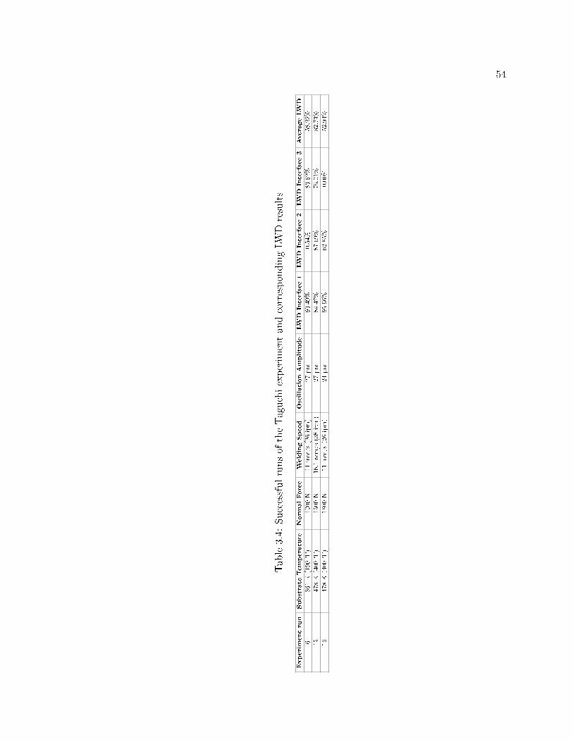
54
Table3.4:
Successfulrunsof
theTaguchiexperimentandcorrespondingLWDresults
Experimentrun
Substrate
Temperature
Norm
alForce
WeldingSpeed
OscillationAmplitude
LWDInterface1
LWDInterface2
LWDInterface3
AverageLWD
6361K(190
°F)
1000
N11
mm/s
(26ipm)
27µm
90.49%
0.54%
83.62%
58.22%
15478K(400
°F)
1500
N16.1mm/s
(38ipm)
27µm
84.47%
87.69%
76.01%
82.73%
16478K(400
°F)
1800
N11
mm/s
(26ipm)
24µm
95.96%
62.85%
0.00%
52.94%
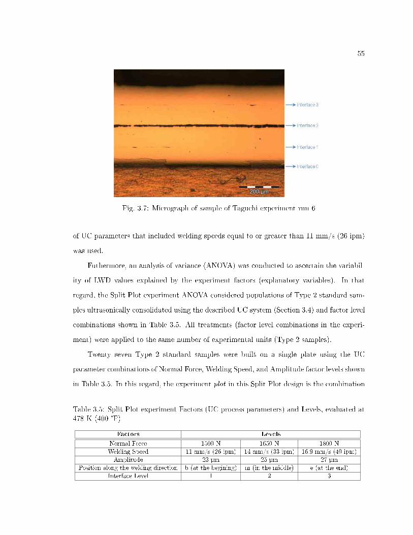
55
Fig. 3.7: Micrograph of sample of Taguchi experiment run 6
of UC parameters that included welding speeds equal to or greater than 11 mm/s (26 ipm)
was used.
Futhermore, an analysis of variance (ANOVA) was conducted to ascertain the variabil-
ity of LWD values explained by the experiment factors (explanatory variables). In that
regard, the Split Plot experiment ANOVA considered populations of Type 2 standard sam-
ples ultrasonically consolidated using the described UC system (Section 3.4) and factor level
combinations shown in Table 3.5. All treatments (factor level combinations in the experi-
ment) were applied to the same number of experimental units (Type 2 samples).
Twenty seven Type 2 standard samples were built on a single plate using the UC
parameter combinations of Normal Force, Welding Speed, and Amplitude factor levels shown
in Table 3.5. In this regard, the experiment plot in this Split Plot design is the combination
Table 3.5: Split Plot experiment Factors (UC process parameters) and Levels, evaluated at478 K (400 °F)
Factors Levels
Normal Force 1500 N 1650 N 1800 N
Welding Speed 11 mm/s (26 ipm) 14 mm/s (33 ipm) 16.9 mm/s (40 ipm)
Amplitude 23 µm 25 µm 27 µmPosition along the welding direction b (at the begining) m (in the middle) e (at the end)
Interface Level 1 2 3

56
Fig. 3.8: Micrograph of sample of Taguchi experiment run 15
of these three experimental factors. For each Type 2 sample in the plot, three di�erent evenly
spaced cross sections were evaluated corresponding to the begining, the middle, and the end
positions along the welding direction in the ultrasonically consolidated section (Figure 3.10).
Five hundred micron wide cross section micrographs were taken at 100X magni�cation as
shown in Figure 3.10, whenever edge e�ects ceased towards the center of the ultrasonically
consolidated section.
In addition, as illustrated in Figure 3.6, there are three SS316L annealed-to-SS316L an-
nealed interfaces (Interface Level factor levels) at each location, thus resulting in 3 Positions×
3 Interfaces = 9 LWD measurements associated with each Type 2 standard sample. The
combination of Position along the Welding Direction and Interface Level factors is the sub-
plot in this Split Plot design. Similarly, by multiplying the number of all factor levels present
in Table 3.5, there are 3× 3× 3× 3× 3 = 243 observations per Plot. There were three repli-
cates per plot or trial run, for a total of 243× 3 = 729 LWD measurements. Experimental
runs are shown in Table 3.6.
The ANOVA was carried out using SAS� statistical software and a critical probability
value of 0.05 was used. Preliminary full �fth order interaction ANOVA results showed that
only interactions of third order or less were signi�cant, and it was decided to use a modi�ed
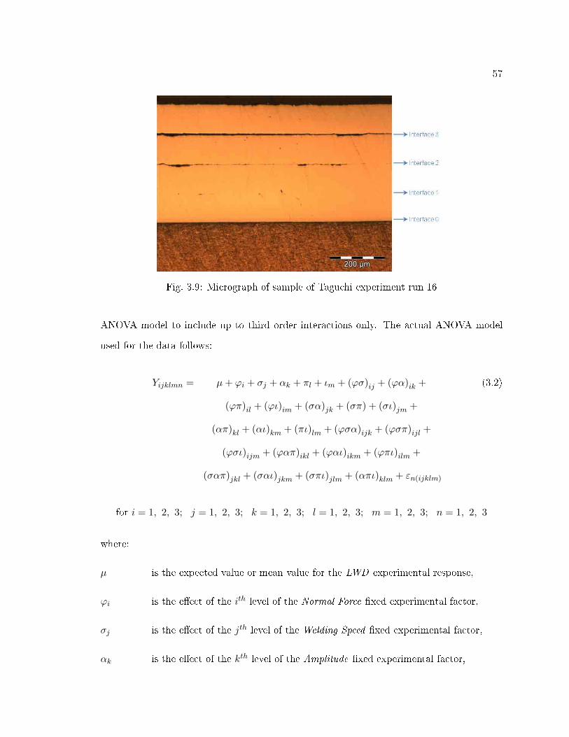
57
Fig. 3.9: Micrograph of sample of Taguchi experiment run 16
ANOVA model to include up to third order interactions only. The actual ANOVA model
used for the data follows:
Yijklmn = µ+ ϕi + σj + αk + πl + ιm + (ϕσ)ij + (ϕα)ik + (3.2)
(ϕπ)il + (ϕι)im + (σα)jk + (σπ) + (σι)jm +
(απ)kl + (αι)km + (πι)lm + (ϕσα)ijk + (ϕσπ)ijl +
(ϕσι)ijm + (ϕαπ)ikl + (ϕαι)ikm + (ϕπι)ilm +
(σαπ)jkl + (σαι)jkm + (σπι)jlm + (απι)klm + εn(ijklm)
for i = 1, 2, 3; j = 1, 2, 3; k = 1, 2, 3; l = 1, 2, 3; m = 1, 2, 3; n = 1, 2, 3
where:
µ is the expected value or mean value for the LWD experimental response,
ϕi is the e�ect of the ith level of the Normal Force �xed experimental factor,
σj is the e�ect of the jth level of the Welding Speed �xed experimental factor,
αk is the e�ect of the kth level of the Amplitude �xed experimental factor,
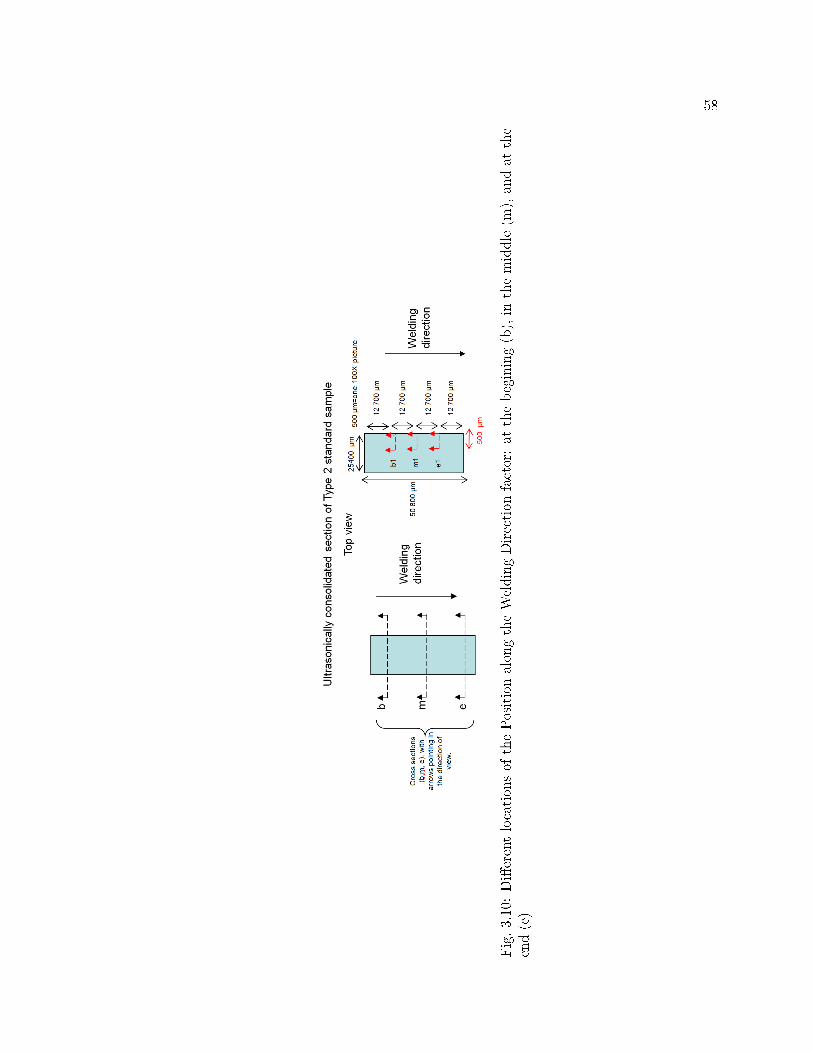
58
Fig.3.10:Di�erentlocationsof
thePositionalongtheWeldingDirection
factor:at
thebegining(b),in
themiddle(m
),andat
the
end(e)

59
πl is the e�ect of the lth level of the Position along the welding direction �xed
experimental factor,
ιm is the e�ect of the mth level of the Interface Level �xed experimental factor,
εn(ijklm) is the random error on the nth trial, and
Yijkl is the response value, namely LWD, for the nth trial, given at the mth level of
the Interface Level , the lth level of the Position along the welding direction, the
kth level of the Amplitude, the jth level of the Welding Speed, and the ith level
of the Normal Force.
All other terms denote interactions of respective factor levels. The Null Hypothesis (H0)
and Alternative Hypothesis (HA) are, respectively:
H0 : ϕ1 = ϕ2 = ϕ3 = 0 (3.3)
σ1 = σ2 = σ3 = 0
α1 = α2 = α3 = 0
π1 = π2 = π3 = 0
ι1 = ι2 = ι3 = 0
HA : At least one ϕi 6= 0 (3.4)
At least one σj 6= 0
At least one αk 6= 0
At least one πl 6= 0
At least one ιm 6= 0
In addition, the ANOVA model is Univariate, because there is only one response or
dependent variable, and all factors are considered crossed with respect to all the others.
Type 3 tests for �xed e�ects are performed for all factors and interactions and the residual

60
maximum likelihood (REML) method is used to estimate components of variance. As for
ANOVA assumptions examination, data residuals are evaluated �rst. In a statistical con-
text, the residual is the deviation of an observation from the estimated true function value,
therefore, it is an estimator of the statistical (random) error [22]. Moreover, Residuals ver-
sus Explanatory Factors plots are shown in Figure 3.11, and provide evidence of a highly
homoscedastic data. The convention in statistics for homoscedasticity in Residuals versus
Explanatory Factors plots is that there should not be a di�erence in spreads equal to or
greater than �ve times when comparing any pair of factor levels in the same Explanatory
factor plot (the spread is illustrated by the vertical chain of symbols corresponding to each
factor level). Furthermore, the Residuals versus Predicted Values plot for the data in Figure
3.12 also shows signi�cant evidence of homoscedasticity since there is not any clear gradient
pattern (e.g. a megaphone shape) in the plot.
Moreover, all other diagnostics con�rm that the residuals normality assumption is quite
reasonable. For instance, the Residuals versus Normal Percentiles plot illustrated in Figure
3.13 shows a fairly straight line, while the Histogram shown in Figure 3.14, and the Stem-
Leaf plot in Figure 3.15 both support normality based upon graphical correspondence with
the bell-shaped distribution of values. In summary, all diagnostics provide no reason to
invalidate the ANOVA results, in light of the evidence that residuals are normally distributed
according to the mathematical theory of errors [22].
As stated in Equation 3.3, the Null Hypothesis (H0) postulated that there was no e�ect
due to the any of the factors on the LWD value, meaning that the distributions of the mean,
variance, and shape of all factor-level samples would be identical. In that respect, a p-value
is calculated in order to accept or reject the Null Hypothesis. The p-value is the probability
of obtaining results at least as extreme as the one that was actually observed, assuming that
the Null Hypothesis is true. In our case, since the critical probability value used in this study
is 0.05, it means that the Null Hypothesis would be rejected if a p-value equal to or less
than 0.05 (5% of expected likelihood) is obtained. Moreover, Type 3 F-test are performed to
obtain the p-values shown in Figure 3.16 because the test statistic associated to the p-value
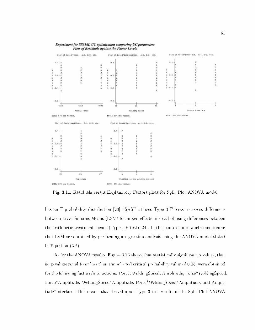
61
Fig. 3.11: Residuals versus Explanatory Factors plots for Split Plot ANOVA model
has an F-probability distribution [23]. SAS� utilizes Type 3 F-tests to assess di�erences
between Least Squares Means (LSM) for mixed e�ects, instead of using di�erences between
the arithmetic treatment means (Type 1 F-test) [24]. In this context, it is worth mentioning
that LSM are obtained by performing a regression analysis using the ANOVA model stated
in Equation (3.2).
As for the ANOVA results, Figure 3.16 shows that statistically signi�cant p-values, that
is, p-values equal to or less than the selected critical probability value of 0.05, were obtained
for the following factors/interactions: Force, WeldingSpeed, Amplitude, Force*WeldingSpeed,
Force*Amplitude, WeldingSpeed*Amplitude, Force*WeldingSpeed*Amplitude, and Ampli-
tude*Interface. This means that, based upon Type 3 test results of the Split Plot ANOVA
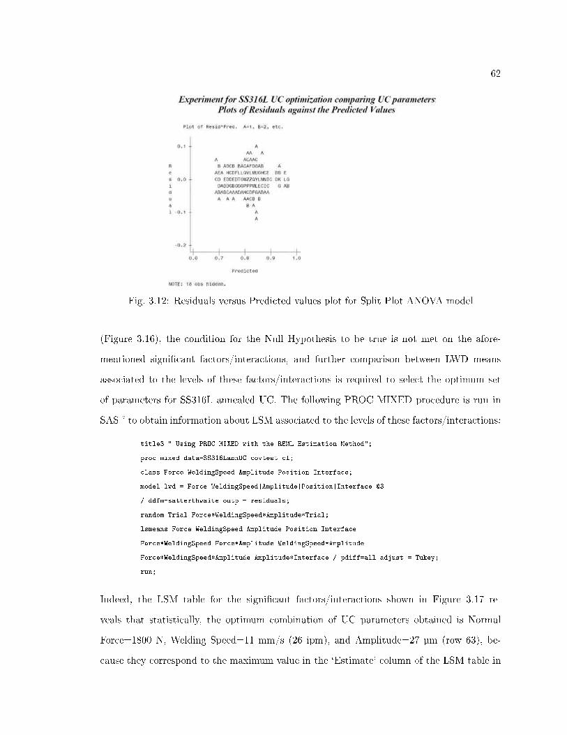
62
Fig. 3.12: Residuals versus Predicted values plot for Split Plot ANOVA model
(Figure 3.16), the condition for the Null Hypothesis to be true is not met on the afore-
mentioned signi�cant factors/interactions, and further comparison between LWD means
associated to the levels of these factors/interactions is required to select the optimum set
of parameters for SS316L annealed UC. The following PROC MIXED procedure is run in
SAS� to obtain information about LSM associated to the levels of these factors/interactions:
title3 " Using PROC MIXED with the REML Estimation Method";
proc mixed data=SS316LannUC covtest cl;
class Force WeldingSpeed Amplitude Position Interface;
model lwd = Force|WeldingSpeed|Amplitude|Position|Interface @3
/ ddfm=satterthwaite outp = residuals;
random Trial Force*WeldingSpeed*Amplitude*Trial;
lsmeans Force WeldingSpeed Amplitude Position Interface
Force*WeldingSpeed Force*Amplitude WeldingSpeed*Amplitude
Force*WeldingSpeed*Amplitude Amplitude*Interface / pdiff=all adjust = Tukey;
run;
Indeed, the LSM table for the signi�cant factors/interactions shown in Figure 3.17 re-
veals that statistically, the optimum combination of UC parameters obtained is Normal
Force=1800 N, Welding Speed=11 mm/s (26 ipm), and Amplitude=27 µm (row 63), be-
cause they correspond to the maximum value in the `Estimate' column of the LSM table in

63
Fig. 3.13: Residuals vs Normal Percentiles plot for Split Plot ANOVA model
Figure 3.17. Furthermore, the Di�erence of Least Squares Means (DLSM) table in Figure
3.18 presents all evaluations involving the optimum parameter set identi�ed for SS316L an-
nealed UC in this study. In this context, the di�erence between LWD means are signi�cant
for all LSM comparisons (the p-values shown in the Pr > |t| column of the DLSM table
are all equal to or less than the 0.05 probability critical value). Therefore, in light of the
statistical evidence presented in Figure 3.18, no other combination of UC parameters in
Table 3.6 provides similar LWD values to the ones found using the indenti�ed optimum UC
parameter set for Type 2 standard samples.
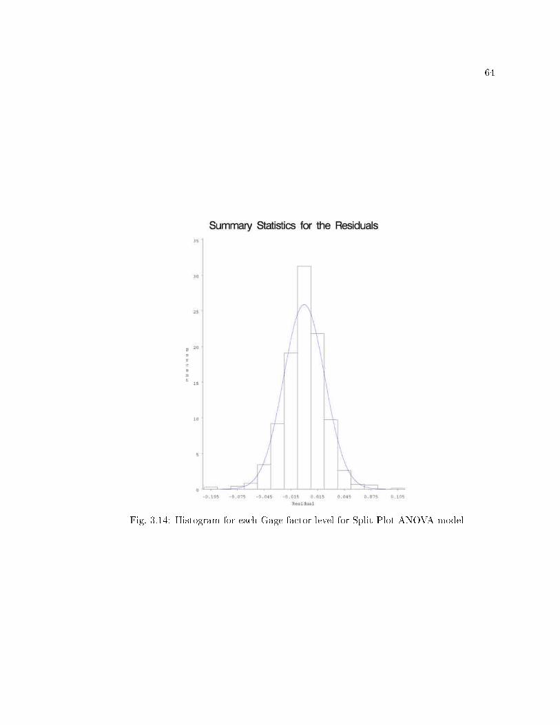
64
Fig. 3.14: Histogram for each Gage factor level for Split Plot ANOVA model
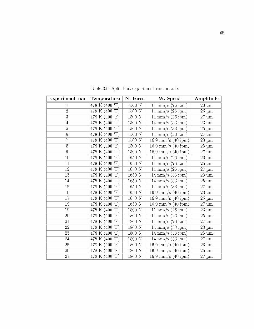
65
Table 3.6: Split Plot experiment runs matrix
Experiment run Temperature N. Force W. Speed Amplitude
1 478 K (400 °F) 1500 N 11 mm/s (26 ipm) 23 µm2 478 K (400 °F) 1500 N 11 mm/s (26 ipm) 25 µm3 478 K (400 °F) 1500 N 11 mm/s (26 ipm) 27 µm4 478 K (400 °F) 1500 N 14 mm/s (33 ipm) 23 µm5 478 K (400 °F) 1500 N 14 mm/s (33 ipm) 25 µm6 478 K (400 °F) 1500 N 14 mm/s (33 ipm) 27 µm7 478 K (400 °F) 1500 N 16.9 mm/s (40 ipm) 23 µm8 478 K (400 °F) 1500 N 16.9 mm/s (40 ipm) 25 µm9 478 K (400 °F) 1500 N 16.9 mm/s (40 ipm) 27 µm10 478 K (400 °F) 1650 N 11 mm/s (26 ipm) 23 µm11 478 K (400 °F) 1650 N 11 mm/s (26 ipm) 25 µm12 478 K (400 °F) 1650 N 11 mm/s (26 ipm) 27 µm13 478 K (400 °F) 1650 N 14 mm/s (33 ipm) 23 µm14 478 K (400 °F) 1650 N 14 mm/s (33 ipm) 25 µm15 478 K (400 °F) 1650 N 14 mm/s (33 ipm) 27 µm16 478 K (400 °F) 1650 N 16.9 mm/s (40 ipm) 23 µm17 478 K (400 °F) 1650 N 16.9 mm/s (40 ipm) 25 µm18 478 K (400 °F) 1650 N 16.9 mm/s (40 ipm) 27 µm19 478 K (400 °F) 1800 N 11 mm/s (26 ipm) 23 µm20 478 K (400 °F) 1800 N 11 mm/s (26 ipm) 25 µm21 478 K (400 °F) 1800 N 11 mm/s (26 ipm) 27 µm22 478 K (400 °F) 1800 N 14 mm/s (33 ipm) 23 µm23 478 K (400 °F) 1800 N 14 mm/s (33 ipm) 25 µm24 478 K (400 °F) 1800 N 14 mm/s (33 ipm) 27 µm25 478 K (400 °F) 1800 N 16.9 mm/s (40 ipm) 23 µm26 478 K (400 °F) 1800 N 16.9 mm/s (40 ipm) 25 µm27 478 K (400 °F) 1800 N 16.9 mm/s (40 ipm) 27 µm

66
Fig. 3.15: Stem and Leaf plot and Boxplot for each Gage factor level for Split Plot ANOVAmodel
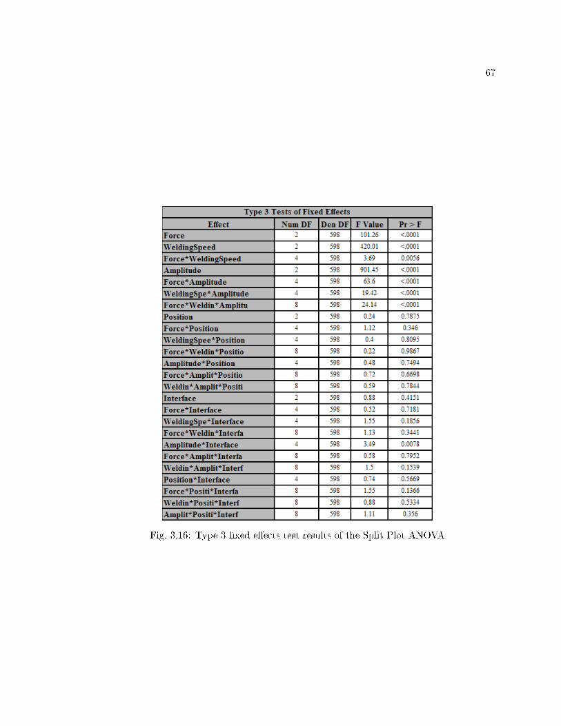
67
Fig. 3.16: Type 3 �xed e�ects test results of the Split Plot ANOVA

68
Fig. 3.17: Least Square Means table of the Split Plot ANOVA

69
Fig.3.18:Di�erence
ofLeast
SquareMeansinvolvingtheoptimum
param
eter
setfoundforSS316L
annealedUCin
theSplitPlot
ANOVA

70
Micrographs of the Type 2 samples made using the optimum parameter set found in
the Split Plot experiment are shown in Figures 3.19, 3.20, and 3.21.
3.6 Discussion
In this study, an optimum combination of UC parameters was obtained at Normal
Force=1800 N, Welding Speed=11 mm/s (26 ipm), and Amplitude=27 µm, by evaluating
factors and levels in Table 3.5 independently from part-geometry induced e�ects. Even
though SS316L UC feasibility studies have been performed in the past [1], LWD has not
been the experimental response in any previous study of SS316L UC. Since other frictional-
related conditions in the UC process were not researched in this study, the optimum SS316L
UC parameter set identi�ed in this work is representative of only the frictional conditions
between the SS316L annealed foils and the sonotrode described above. If these frictional
conditions change signi�cantly, as it may be the case with a di�erent sonotrode size/material,
sonotrode wear over time, di�erent foil material/thickness and di�erent UC system, then
new optimum UC process parameters should be established. For this reason, this UC study
included speci�c sonotrode surface roughness data (Table 3.1) for reference.
Nonetheless, the present work independently veri�ed that bond formation during ultra-
sonic consolidation of SS316L annealed can be obtained consistently. Moreover, the Split
Plot ANOVA results provides evidence of the e�ect the factors/interactions shown in Table
3.5 have on SS316L annealed UC. For instance, both Interface Level and Position along
welding direction factors were not signi�cant for LWD values on Type 2 standard samples.
Additionally, although not part of the Split Plot ANOVA, Temperature is a signi�cant factor
in SS316L annealed UC processing because bonding was achieved far more consistently at
478 K (400 °F) than at 303 K (85 °F) over the same number of trials. Successful depositions
were obtained at all Welding Speed con�gurations tested and shown in Table 3.6. In simil-
itude with Al 3003 UC [10], Oscillation Amplitude was proven to be in�uential in SS316L
annealed UC. Indeed, it was observed that the LWD of Type 2 standard samples tends to
increase with higher Amplitudes, as reported previously in literature [1].
All in all, the experimental results presented as part of this work reveal some important

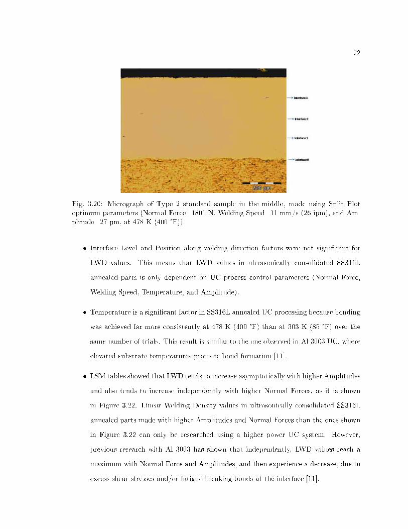
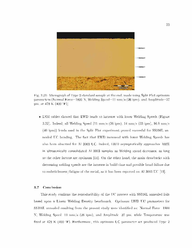
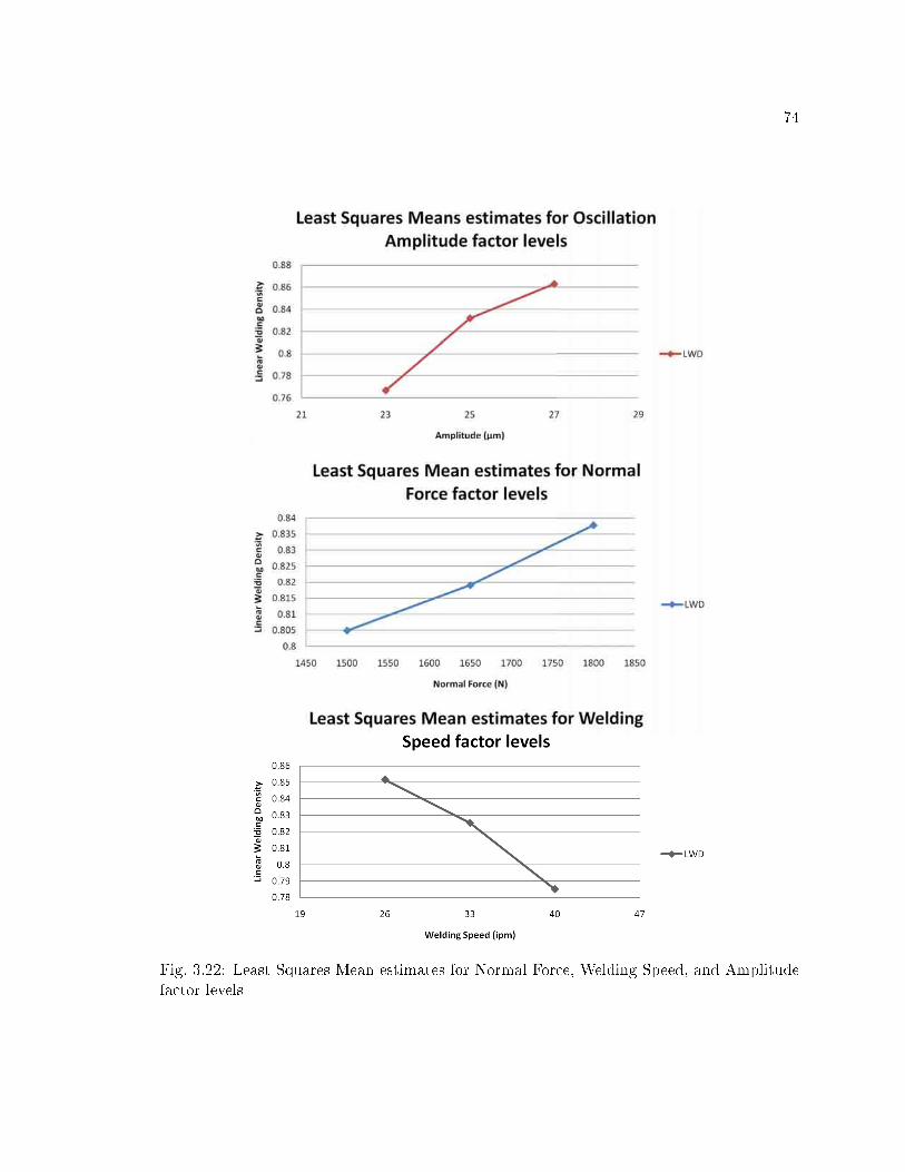
75
standard samples with an estimated Least Square Mean LWD value of 95.89%. Although the
maximum LWD parameter set found may not be the global optimum for SS316L annealed
UC due to uninvestigated results with higher power UC machines, the LWD values obtained
using the optimum parameter set for SS316L annealed are comparable to the maximum
LWD values found for Al 3003 [11], and thus the optimum parameter set is very acceptable
for structural part fabrication.
3.8 Future Work
Further experiments at lower welding speeds than 11 mm/s (26 ipm) with other factor
levels �xed can provide additional information about the SS316L annealed UC process on
the UC system utilized in this study. Although Welding Speed can be set arbitrarily low,
this particular factor presents a clear trade-o� between LWD and part build time [11]. In
addition, studies involving interface microstructural analysis are necessary to explore SS316L
annealed crystallography in the interface region of ultrasonically consolidated layers.
Per consideration of the fact that maximum allowable settings for Normal force and
Amplitude were employed to obtain the optimum UC parameter set for SS316L annealed in
the available UC system, it is deemed that a more powerful UC system may enable further
evaluation of UC of SS316L annealed foils beyond the optimum parameter set obtained
in this study. Higher power UC systems could be employed to perform a more general
optimization experiment for SS316L annealed UC, and explore part-geometry induced e�ects
like overhanging, ribbed, or near-corner con�gurations, and height-to-width ratio limits.

76
Chapter 4
Overall Conclusions
Ultrasonically consolidated structures with enhanced strength, rigidity, and sti�ness are
one signi�cant step towards the practical application of Ultrasonic Consolidation (UC) tech-
nology. This dissertation has investigated the e�ect of UC process parameters on Stainless
Steel 316L (SS316L) annealed foils based upon a Linear Welding Density (LWD) bench-
mark. Along this research e�ort, a new instrument for LWD estimation on ultrasonically
consolidated samples has been developed, and a Measuring System Analysis of LWD as-
sessment has been performed. The knowledge and understanding achieved in the current
study provides a clear understanding of the issues involved in the application of UC to the
fabrication of SS316L annealed structures.
4.1 MATLAB Script for LWD Estimation through Image Processing
The assessment of LWD is an important benchmark to characterize UC bond quality on
SS316L samples. In fact, certain properties of SS316L annealed ultrasonically consolidated
parts could only be speci�ed once UC bond quality is known. For instance, properties like
speci�c weight and Poisson's ratio of ultrasonically consolidated parts are a�ected by LWD.
The MATLAB script presented in this study o�ers a computer-assisted method for assessing
LWD. The method presented is based upon the application of image processing techniques
on a single metal to metal interface picture for LWD assessment, using a picture brightness
criteria. A step-by-step guide to the MATLAB script is included in the Appendix.
The experimental results presented show that the MATLAB script can e�ectively esti-
mate LWD on cross section micrographs. Results from the Measurement System Analysis
of Variance of LWD instruments performed indicate that: (1) The MATLAB script provides
the highest instrument resolution of all LWD measuring instruments. (2) The MATLAB

77
script can accurately and reliably reproduce traditional Ruler-based methods based upon
the image �le and Region of Interest information. (3) The spread of LWD measurements
using the MATLAB script is less than the spread associated with the Ruler and GIMP
Measure Tool instruments, making the MATLAB script the most suitable as a standard
LWD measurement tool of the three instruments evaluated in this work. Measuring Sys-
tem ANOVA results also show the MATLABsc measurement system is e�cient in assessing
LWD. The average time per user per sample to take LWD measurements (in seconds) using
the MATLAB script is 46.36% less than that of the Ruler and 57.70% less than that of the
GIMP.
Although there are some limitations for the Image Processing approach used in the
MATLAB script routine, they are mostly related to the single horizontal interface conser-
vative analysis paradigm implemented and micrograph optical requirements. In order to
use the MATLAB script properly, high quality micrographs and level of sample preparation
(grinding and polishing) are required. In turn, it has been observed that aside poor sample
preparation and/or microscopy, the MATLAB script can estimate LWD on high contrast
cross section micrographs on a reproducible basis. Tested results show that grinding and
polishing of ultrasonically consolidated samples must be performed down to a grit size equal
or lower than 6.5 microns in average particle size.
That being said, it is worth mentioning that the MATLAB script can be used to perform
LWD measurements on micrographs including multiple interfaces, although at its current
stage, the procedure can only process one interface per run. It is important to set an adequate
magni�cation level for sample microscopy. For picture-wide interfaces, the recomended
magni�cation level range for de�ning the ROI to obtain a LWD estimate using the MATLAB
script is 50-100X. Based on several tests performed, some defects could not be clearly seen
inside the MATLAB �gure window with a microscopy magni�cation level lower than 50X,
without zoom. At the other end, picture-wide interfaces do not have enough interface
length for proper analysis when using microscopy magni�cation levels above 100X. For ROI
de�nitions that are not picture-wide, the zoom option available in the MATLAB script

78
routine can be used with magni�cation levels above 100X and below 50X, and the practical
minimum/maximum magni�cation for microscopy will depend upon the speci�c application.
The MATLAB script procedure is designed to work with only one micrograph. Multiple
or combined image analysis using the MATLAB script is only indirectly possible at this
development point, by stitching together multiple side-by-side micrographs to make a single
micrograph of an horizontally oriented contiguous interface, for futher analysis.The latest
version of the MATLAB script can be downloaded from:
https://sites.google.com/site/lwdmatlabsc/
4.2 Maximum LWD UC Parameters for SS316L Annealed UC
The quality of an ultrasonically consolidated part is highly dependent on UC processing
parameters. From a research standpoint, the relevance of this research e�ort consists in a
systematic study of SS316L annealed UC based on the relation between UC parameters and
resulting LWD values on samples, independent from part geometry induced e�ects. There
are four machine-related processing parameters in an UC system: Oscilation Amplitude,
Welding Speed, Normal Force and Substrate Temperature. Besides these four machine-
related parameters, this research project included two additional factors to be considered,
which are the Position along the welding direction and the Interface Level. Speci�cally,
maximum LWD UC parameters for SS316L annealed parts using the available UC system
were identi�ed at: Normal Force=1800 N, Welding Speed=11 mm/s (26 ipm), and Ampli-
tude=27 µm, while Temperature was �xed at 478 K (400 °F). Furthermore, SS316L annealed
standard samples produced with the identi�ed optimum UC parameter set yielded nearly
96% of LWD.
This study has experimentally investigated the e�ects of processing parameters on UC
bond quality in SS316L annealed structures using a LWD criteria and has identi�ed opti-
mum levels for UC parameters. On the other hand, frictional-related conditions in the UC
process were not researched in this study. In consequence, the optimum SS316L UC param-
eter set identi�ed in this work is representative of a restricted range of frictional conditions
between the SS316L annealed foils and the sonotrode. If these frictional conditions change

79
signi�cantly, as it may be the case with a di�erent sonotrode size/material, sonotrode wear
over time, di�erent foil material/thickness and di�erent UC system, then new optimum UC
process parameters should be established, and speci�c sonotrode surface roughness data
should be recorded for reference. Nonetheless, the present work independently veri�ed that
bond formation during ultrasonic consolidation of SS316L annealed can be obtained con-
sistently. Moreover, the Split Plot ANOVA results provide evidence of the e�ect the UC
parameter factors/interactions have on SS316L annealed UC. For instance, both Interface
Level and Position along welding direction factors were not related to LWD values on stan-
dard samples. In turn, although it was not part of the Split Plot ANOVA, Temperature
is a signi�cant factor in SS316L annealed UC process because bonding was achieved far
more consistently at 478 K (400 °F) than at 303 K (85 °F) over the same number of trials.
Successful depositions were obtained at Welding Speed of 11 mm/s (26 ipm), 14 mm/s (33
ipm), and 16.9 mm/s (40 ipm), but the complete process parameter window of Welding
speeds was not fully explored on the available UC system in this study.
All in all, the experimental results presented as part of this work reveal some impor-
tant trends for the SS316L annealed UC process. Experiment outcomes on ultrasonically
consolidated SS316L annealed parts indicated that only variations in Oscilation Amplitude,
Welding Speed, Normal Force and Substrate Temperature produce statistically signi�cant
variations in LWD values. Speci�cally, it was observed that higher values of Oscillation
Amplitude, Normal Force, and Substrate Temperature respectively resulted in higher LWD
values, whereas Welding Speed was found to a�ect LWD in the opposite manner: The higher
the Welding Speed, the smaller the LWD produced. Speci�cally, the optimum parameter
set obtained as part of the Split Plot ANOVA includes maximum settings for Normal Force
and Amplitude for the UC system utilized. This clearly suggests the acoustic energy nec-
essary for SS316L annealed UC is greater than that for Al 3003 UC, and indicates that a
more powerful UC system is needed to examine the full potential of SS316L annealed UC.
Even with the available UC system limitations, UC of SS316L annealed was con�rmed with
LWD values comparable to those found for Al 3003/6061 UC previously. Further machine
80
improvements that enable larger Oscillation Amplitudes, higher Normal Forces, and higher
temperatures may enable UC of SS316L annealed foils with higher LWD values than the
one obtained for the optimum in this study.
4.3 Future Work
Regarding the MATLAB script, future work includes the need to improve the robustness
of the MATLAB script procedure for e�cient identi�cation of sample defects (voids, delam-
ination, inclusions) and LWD assessment. Also, an option for processing multiple interfaces
in one micrograph will be incorporated in order to provide an average LWD estimate for
all interfaces in a micrograph. However, it has been noted that a complete LWD measure-
ment standard would require additional work, including speci�c information about minimum
requirements for the optical system (used to acquire ultrasonically consolidated sample mi-
crographs), and weldment preparation in terms of preparation times, speci�c preparation
materials/equipment, and preparation methods in tandem with the ultrasonically consoli-
dated material used and the level of quality desired.
Future work related to SS316L annealed UC includes mechanical characterization and
mechanical properties testing for SS316L annealed ultrasonically consolidated samples. Per
consideration of the fact that maximum allowable settings for Normal force and Ampli-
tude were employed to obtain the optimum UC parameter set for SS316L annealed in the
available UC system, it is posited that a more powerful UC system may enable further eval-
uation of UC of SS316L annealed foils beyond the optimum parameter set obtained in this
study. In addition to this, further experiments at lower Welding Speeds than 11 mm/s (26
ipm) with other factor levels �xed can provide additional information about the SS316L an-
nealed UC process on the UC system utilized in this study. Higher power UC systems could
be employed to perform a more general optimization experiment for SS316L annealed UC,
and explore part-geometry induced e�ects like overhanging, ribbed, or near-corner con�gura-
tions, and height-to-width ratio limits. Moreover, studies involving interface microstructural
analysis are necessary to explore SS316L annealed crystallography in the interface region of
ultrasonically consolidated layers.

81
References
[1] Tuttle, R. B., 2007, �Feasibility study of 316L stainless steel for the ultrasonic consoli-
dation process,� Journal of Manufacturing Processes, 9(2), pp. 87�93.
[2] Weiss, B., and Stickler, R., 1972, �Phase instabilities during high temperature exposure
of 316 austenitic stainless steel,� Metallurgical and Materials Transactions B, 3, pp.
851�866.
[3] Davies, D., Adcock, P., Turpin, M., and Rowen, S., 2000, �Stainless steel as a bipolar
plate material for solid polymer fuel cells,� Journal of Power Sources, 86, pp. 237�242.
[4] Hernandez, L. A., 2009, �Integration of ultrasonic consolidation and direct-write to
fabricate an embedded electrical system within a metallic enclosure,� Master's thesis,
Utah State University, Logan, UT, USA.
[5] Yang, Y., Ram, G. D. J., and Stucker, B. E., 2007, �An experimental determination
of optimum processing parameters for Al/SiC metal matrix composites made using
ultrasonic consolidation,� Journal of Engineering Materials and Technology, 129, pp.
538�549.
[6] Daniels, H. P. C., 1965, �Ultrasonic welding,� Ultrasonics, 3(4), pp. 190�196.
[7] Ram, G. J., Y. Yang, C. R., J. George, and Stucker, B., 2006, �Improving linear weld
density in ultrasonically consolidated parts,� Proceedings of the 17th Solid Freeform
Fabrication Symposium, pp. 692�708.
[8] Zhang, C., Zhu, X., and Li, L., 2006, �A 3-D coupled-�eld dynamic model for ultrasonic
welding of aluminum foils,� Materials Science & Technology 2006, Symp. on Joining of
Advanced and Specialty Materials Including A�ordable Joining of Titanium and Joining
Technologies for MMCs.

82
[9] Kong, C. Y., Soar, R. C., and Dickens, P. M., 2003, �Characterisation of aluminium
alloy 6061 for the ultrasonic consolidation process,� Materials Science and Engineering
A, 363(1-2), pp. 99�106.
[10] Kong, C. Y., Soar, R. C., and Dickens, P. M., 1991, �Optimum process parameters for
ultrasonic consolidation of 3003 aluminum,� Journal of Materials Processing Technol-
ogy, 146, pp. 181�187.
[11] Ram, G. J., Yang, Y., and Stucker, B., 2007, �E�ect of process parameters on bond
formation during ultrasonic consolidation of aluminum alloy 3003,� Journal of Manu-
facturing Systems, 25(3), pp. 221�238.
[12] Robinson, C. J., 2005, �Integration of ultrasonic consolidation and direct-write to fab-
ricate a mini-sar phased array antenna,� Master's thesis, Utah State University, Logan,
UT, USA.
[13] Kong, C., Soar, R., and Dickens, P., 2002, �An investigation of the control parameters for
aluminum 3003 under ultrasonic consolidation,� Proceedings of the 13th Solid Freeform
Fabrication Symposium, pp. 199�210.
[14] Stanley J. Reeves, �MATLAB for digital image processing,�
http://www.eng.auburn.edu/ sjreeves/Classes/IP/IP.html (Last accessed: November
17th, 2009).
[15] Otsu, N., 1979, �A threshold selection method from gray-level histograms,� IEEE Trans-
actions on Systems, Man and Cybernetics, 9(1), pp. 62�66.
[16] Morse, B. S., 2000, �Lecture 4: Thresholding,�
http://www.eng.auburn.edu/ sjreeves/Classes/IP/IP.html (Last accessed: December
1st, 2009).
[17] Sydenham, P., and Thorn, R., eds., 2005, Handbook of Measuring System Design: Com-
mon Sources of Errors in Measurement Systems, Wiley, pp. 1-6.
83
[18] Senol, S., 2004, �Measurement system analysis using designed experiments with mini-
mum α-β Risks and n,� Measurement, 36(2), pp. 131�141.
[19] Krishnamoorthi, K. S., 2006, A �rst course in quality engineering: integrating statistical
and management methods of quality, Prentice-Hall, Upper Saddle River, NJ, pp. 234�
246.
[20] Leon, R., and Mee, R., 2000, �Blocking multiple sources of error in small analytic
studies,� Quality Engineering, 12, pp. 497�501.
[21] Simion, C., 2005, �The study of a measurement system precision,� 13th International
Scienti�c Conference on Achievements in Mechanical and Materials Engineering, pp.
585�588.
[22] Cook, R. D., and Weisberg, S., 1982, Residuals and In�uence in Regression, Springer,
New York, NY, pp. 10-93.
[23] Oehlert, G. W., 2000, A �rst course in design and analysis of experiments, W. H.
Freeman, New York, NY, pp 323-455.
[24] SAS, 2004, SAS/STAT 9.1 user's guide: The MIXED Procedure, SAS Publishing, Cary,
NC, pp. 2661-2844.
[25] Huang, Q., Gao, W., and Cai, W., 2005, �Thresholding technique with adaptive window
selection for uneven lighting image,� Pattern Recognition Letters, 26, pp. 801�808.
[26] Robinson, C., Zhang, C., Ram, G. J., Siggard, E., Stucker, B., and Li, L., 2006, �Max-
imum height to width ratio of freestanding structures built using ultrasonic consolida-
tion,� Proceedings of 17th Solid Freeform Fabrication Symposium.
[27] Doumanidis, C., and Gao, Y., 2004, �Mechanical modeling of ultrasonic welding,� Weld-
ing Journal, 83, pp. 140�146.
[28] Zhang, C., and Li, L., 2006, �A study of dynamic mechanical behavior of substrate in
ultrasonic consolidation,� Proceedings of 17th Solid Freeform Fabrication Symposium.

84
[29] Zhang, C., Zhu, X., and Li, L., 2006, �A study of friction behavior in ultrasonic welding
(consolidation) of aluminum,� 87th FABTECH International and AWS Welding Show
Professional Program.
[30] Yang, Y., Ram, G. J., and Stucker, B., 2010, �Mechanical properties & microestructures
of SiC �ber reinforced metal matrix composites made using ultrasonic consolidation,�
Journal of Composite Materials, In press.
[31] Roy, R. K., 2001, Design of Experiments Using the Taguchi Approach: 16 Steps to
Product and Process Improvement, Wiley, John & Sons, Inc., New York, NY, pp. 95-
206.

85
Appendix

86
Appendix
A.1 MATLAB Script Supplement
A.1.1 How to Obtain the MATLAB Script
The latest version of the MATLAB script is available for free under the terms contained
in the lwd.m script �le and can be downloaded from:
https://sites.google.com/site/lwdmatlabsc/
A.1.2 MATLAB Script User Guide
A MATLAB script, `lwd.m', was developed to assess LWD in cross section micrographs
of weldments. The method is based upon the use of a set of image processing techniques
that, when combined, provide a single metal to metal interface LWD assessment. The
MATLAB script takes for an input a rectangular region of the cross section micrograph, and
provided this region contains the interface of interest and meets standard metallography
quality criterias, the tool can provide an automatic estimation of the LWD present at the
interface. Either grayscale or color images can be processed, in both Bitmap (bmp) and
Tagged Image File (tif) formats. The most fundamental assumption of the MATLAB script
program is that darker areas in the micrograghs represent unbonded areas, and thus, it is
dependent upon the brightness of the visual target. On the other hand, in order to use the
MATLAB script for LWD assessment, the interface shown in the cross section micrograph
must be horizontally oriented, in focus, and the sample must be in not-etched, scratchless,
and as-polished conditions. An examination of these and other conditions that a�ect LWD
assessment using the MATLAB script are given in the Discussion section of this work.
The MATLAB script works in MATLAB version 7.0 (R14) or newer, with the Image
Processing Toolbox installed. The routine is executed inside the MATLAB command win-
dow, and prompts for an image �lename �rst. Figure A.1 shows an example of how an image

87
Fig. A.1: File input example in MATLAB script
�le that has already been placed in the MATLAB working directory, namely `sample1.bmp',
is entered as input. Upon specifying this image �le (by entering the �lename including the
�le extension), the actual image is shown on screen as a �gure and the program waits for
the user's con�rmation on the image. In this regard, Ctrl+c will abort the operation and
any other standard keystroke will proceed with analysis.
Following this, the rectangular Region of Interest (ROI) needs to be de�ned by the user.
The Region of Interest is the smallest rectangular region, or subset of the original image, that
contains all relevant pixels depicting the interface of interest. In this manner, the Region
of Interest is a graphical representation of the interface in the form of a rectangle and its
contents. Furthermore, all image processing operations are performed on the Region of
Interest de�ned by the user. Figure A.2 illustrates the image, the target interlayer interface,
and a selected Region of Interest in the sample1.bmp image �le.
The Region of Interest is de�ned by the user, using either Visual Clicks, Matrix Coor-
dinates, or Relative Coordinates.
The Visual Clicks approach comprises two click-points so as to de�ne the Region of
Interest with the aid of a pointing device. These separate clicks specify the rectangle con-

88
Fig. A.2: Image, Interlayer Interface, and Region of Interest illustrations
taining the Region of Interest, by de�ning two rectangle corners diagonally opposite. If
the interface extends all across the image, then clicks can be performed outside the image's
border but inside the MATLAB �gure window. In that way, the script program will adjust
the selection to meet the border or borders of the image accordingly. The Visual Clicks
approach is the default option. Figure A.4 illustrates the Visual Clicks approach, showing
the points where clicks could be performed to select a Region of Interest for the interface
shown.
The second option for de�ning the Region of Interest is Matrix Coordinates. Matrix
Coordinates are based upon the matrix representation of an image in MATLAB, called the
Fig. A.3: Options menu to de�ne the Region of Interest in the MATLAB script

89
Fig. A.4: Visual Clicks approach to de�ne the Region of Interest in the MATLAB script
Image Matrix. Moreover, Matrix Coordinates are given in terms of row number and column
number following a standard mathematical matrix scheme. The element at the upper left
corner of the image corresponds to the element at row 1, column 1, in the Image Matrix; with
row number increasing downwards, and column number increasing rightwards. The Region
of Interest is de�ned in Matrix Coordinates by specifying the row and column numbers that
bound a rectangular region. This is ilustrated in Figure A.5.
Relative Coordinates is the third option for de�ning the Region of Interest. Relative
Coordinates are Cartesian Coordinates with the origin placed at the lower left corner of
the original image, and coordinate's dimensions scaled up so that the height and the width
of the original image equals to a unit of distance, respectively. Consequently, coordinated
values for both vertical and horizontal axes of the cartesian system are always relative to
the size of original image, and lay in between 0 and 1. Figure A.6 illustrates the Relative
Coordinates approach.
Once the Region of Interest is de�ned by the user using either Visual Clicks, Matrix

90
Fig. A.5: Matrix Coordinates approach to de�ne the Region of Interest in the MATLABscript
Coordinates, or Relative Coordinates, an image of the Region of Interest is presented to the
user. Figure A.7 shows a Region of Interest selection example.
The Region of Interest is then converted to grayscale using an 8-bit grayscale conversion.
MATLAB supports image processing of grayscale and color images [14], and using this
feature, the Region of Interest is converted to an 8-bit grayscale image (an image comprising
28 = 256 di�erent shades of gray) unless the original image is already in this format. Indeed,
MATLAB functions ind2gray and rgb2gray are used to perform 8-bit grayscale conversion
for indexed and RGB images, respectively, whenever necessary. In order to perform the 8-bit
conversion using the MATLAB script, click on the �gure that shows the Region of Interest
and press Enter (it must be the active window). Figure A.8 illustrate the Region of Interest
after the 8-bit grayscale conversion.
Once the 8-bit grayscaled Region of Interest has been obtained, black and white bina-
rization is performed. The black and white representation of the Region of Interest is based
upon applying the Otsu thresholding algorithm [15] on the 8-bit grayscaled Region of Inter-

91
Fig. A.6: Relative Coordinates approach to de�ne the Region of Interest in the MATLABscript
est. Otsu's algorithm performs black and white binarization by selecting the threshold shade
of gray (intensity of gray) that minimizes the within class variance in the image's grayscale
histogram, when the background (pixels with shades of gray darker than the threshold),
and foreground (all pixels that are not in the background), are considered as histogram
classes [16]. In order to perform the black and white binarization using the MATLAB
script, click on the �gure that shows the 8-bit grayscaled Region of Interest (it must be
the active window) and press Enter. Figure A.9 shows an image of the previous grayscaled
Region of Interest (Figure A.8) after black and white binarization.
Following black and white binarization, each black pixel in black and white representa-
tion of the Region of Interest is projected across the vertical direction, as shown in Figure
A.10. The aim of this image processing task is to consider the worst case scenario of maxi-
mum unbonded (black) pixels per row across the Region of Interest. Black pixel projection
also simpli�es further analysis by making all rows in the resulting image identical.
In MATLAB, color values for black and white colors in an Image Matrix are zeroes and

92
Fig. A.7: Region of Interest example in the MATLAB script
ones respectively, thus providing a means to perform mathematical operations on black and
white images. For this particular case, the color values representing black and white colored
areas will prove useful as they are associated to unbonded and bonded areas, respectively.
For instance, once black pixels are projected vertically, all pixel values in the �rst row
(comprising color values of zeroes and ones) are added up, e�ectively calculating the number
of white pixels in the �rst row. When the total sum of the �rst row of pixels is divided by the
number of pixels in the �rst row and multiplied by 100, an estimate of the LWD is obtained,
as stated in Equation (A.1), that provides the LWD of a given interface using a relation of
lengths:
%LWD =Bonded interface length
Total interface length× 100 (A.1)
The output of the MATLAB script is printed after an estimate of the LWD has been
calculated. The output of the MATLAB script includes the following information regarding
the image �le: LWD value, �lename, original Image Matrix dimensions, 8-bit grayscale
threshold value used, and Matrix Coordinates for the selected Region of Interest. An example
of the output is given in Figure A.11. Since the Region of Interest is given in Matrix
Coordinates as part of the output, and because Matrix Coordinates is one option to de�ne

93
Fig. A.8: 8-bit grayscale conversion of the Region of Interest example in the MATLAB script
the Region of Interest (see Figure A.11), the output of the script e�ectively provides a
transparent way to refer back to previous results and to repeat estimations, whenever the
original �le and the associated MATLAB script output are used.
After each run, the program resumes and prompts for the next image �lename input.
In consequence, the MATLAB script routine allows the sequential �le execution until a stop
signal is entered by pressing Ctrl+c keystroke combination in MATLAB's command window.
A.1.3 Known Limitations of the MATLAB Script
In order to use the MATLAB script as an application on a general basis, it is important
to realize the scope and limitations of this measuring instrument, as it is presented below.
First, one critical step of the script routine is the de�nition of the Region of Interest,
because it is the input on which all further image processing tasks take place. The option
of selecting a Region of Interest for assessing LWD in the MATLAB script allows single
interface speci�cation (in sample micrographs with multiple layers) and provides compu-
tational simpli�cation for further image processing. However, the interface shown in the
Image File input (Figure A.1) must be horizontally oriented, and it is crucial to de�ne

94
Fig. A.9: Illustration of black and white binarization using Otsu thresholding algorithm inthe MATLAB script
the Region of Interest as close as possible to the interface in order to perform a correct
analysis. In this respect, MATLAB has limited dynamic zoom capabilities to facilitate the
selection of the Region of Interest using the Visual Clicks option. Speci�cally, the zoom
in/out option can only be used in the MATLAB script routine when the initial image is
initially shown on screen (Figure A.1), and the zoom magni�cation level cannot be adjusted
afterwards. For this reason, it is also important to set an adequate magni�cation level
for sample microscopy. For picture-wide interfaces, the recommended magni�cation level
range for de�ning the ROI to obtain a LWD estimate using the MATLAB script is 50-100X.
Based on several tests performed, some defects could not be clearly seen inside the MAT-
LAB �gure window with a microscopy magni�cation level lower than 50X, without zoom.
At the other end, picture-wide interfaces do not have enough interface length for proper
analysis when using microscopy magni�cation levels above 100X. For ROI de�nitions that
are not picture-wide, the zoom option available in the MATLAB script routine can be used
with magni�cation levels above 100X and below 50X, and the practical minimum/maximum
magni�cation for microscopy will depend upon the speci�c application.
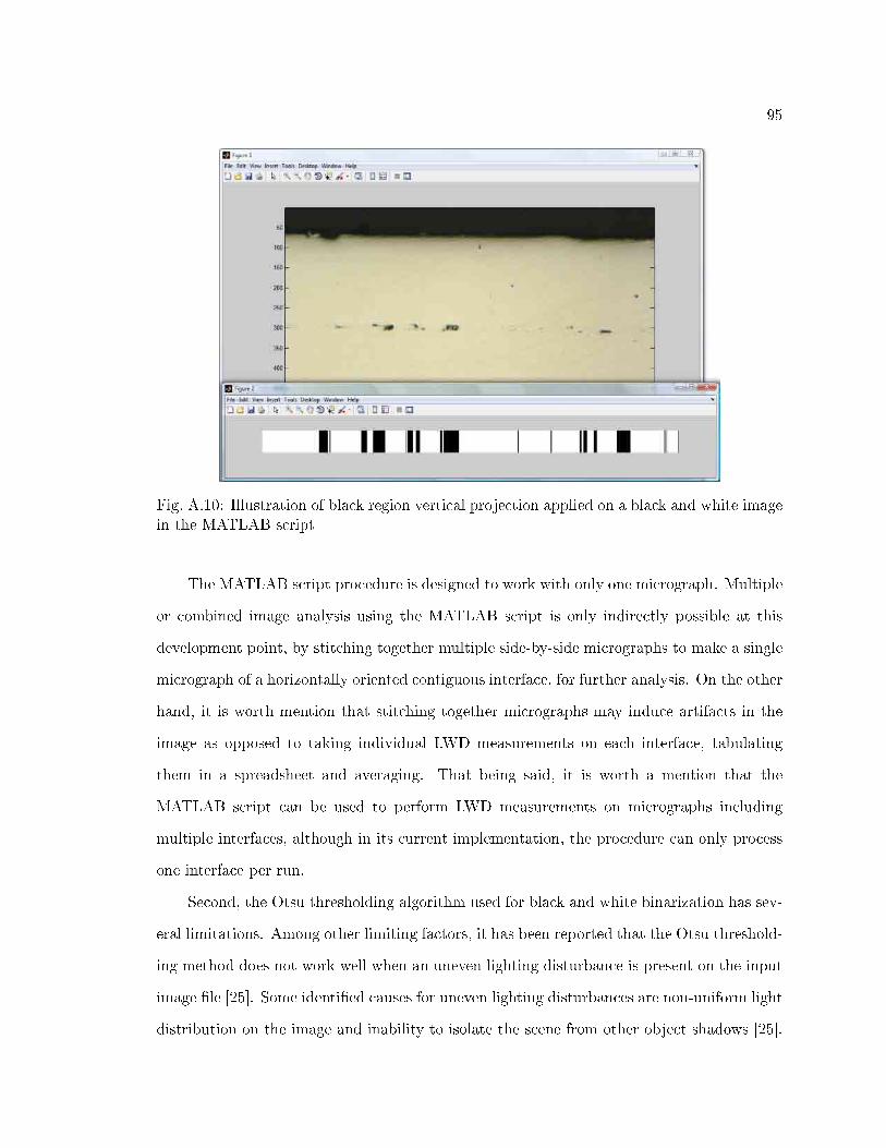
95
Fig. A.10: Illustration of black region vertical projection applied on a black and white imagein the MATLAB script
The MATLAB script procedure is designed to work with only one micrograph. Multiple
or combined image analysis using the MATLAB script is only indirectly possible at this
development point, by stitching together multiple side-by-side micrographs to make a single
micrograph of a horizontally oriented contiguous interface, for further analysis. On the other
hand, it is worth mention that stitching together micrographs may induce artifacts in the
image as opposed to taking individual LWD measurements on each interface, tabulating
them in a spreadsheet and averaging. That being said, it is worth a mention that the
MATLAB script can be used to perform LWD measurements on micrographs including
multiple interfaces, although in its current implementation, the procedure can only process
one interface per run.
Second, the Otsu thresholding algorithm used for black and white binarization has sev-
eral limitations. Among other limiting factors, it has been reported that the Otsu threshold-
ing method does not work well when an uneven lighting disturbance is present on the input
image �le [25]. Some identi�ed causes for uneven lighting disturbances are non-uniform light
distribution on the image and inability to isolate the scene from other object shadows [25].

96
Fig. A.11: MATLAB script output example
In addition to avoiding uneven lightning disturbances, input micrographs with good opti-
cal characteristics (in-focus image, balanced contrast image, adequate depth of �eld (image
sharpness), absence of blurring or image distortions, etc.) are required in order to ensure
accurate LWD assessment by any visual-based method, including the MATLAB script. The
Otsu thresholding routine works best in those ROI that include both bonded and unbonded
areas with clearly di�erent brightness. Despite this, the micrograph quality necessary for
performing accurate black and white binarization using the Otsu method is completely at-
tainable. Based on tests using previous published pictures of ultrasonically consolidated
samples ( [7]), optically unsuitable micrographs are avoided when good sample preparation
(grinding and polishing) and microscopy practices are followed. Experimental results show
that grinding and polishing of ultrasonically consolidated samples must be performed down
to a grit size equal to or lower than 6.5 microns in average particle size.
As for the e�ect of poor sample preparation on MATLAB script LWD results, Figure
A.12 shows a sample micrograph containing scratches and stains, and one 8-bit grayscale
ROI analysis example. Basically, both scratches and stains introduce noise in the Otsu's
thresholding (Black and White binarization) routine that derives into black pixels that do
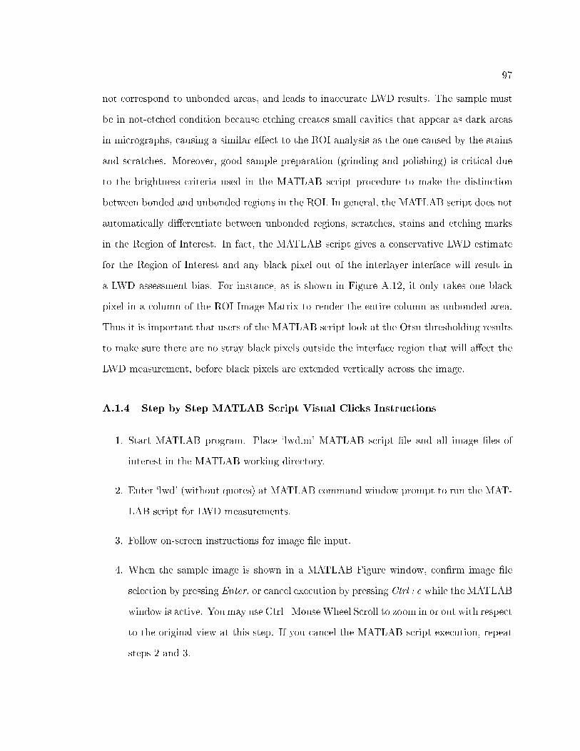
97
not correspond to unbonded areas, and leads to inaccurate LWD results. The sample must
be in not-etched condition because etching creates small cavities that appear as dark areas
in micrographs, causing a similar e�ect to the ROI analysis as the one caused by the stains
and scratches. Moreover, good sample preparation (grinding and polishing) is critical due
to the brightness criteria used in the MATLAB script procedure to make the distinction
between bonded and unbonded regions in the ROI. In general, the MATLAB script does not
automatically di�erentiate between unbonded regions, scratches, stains and etching marks
in the Region of Interest. In fact, the MATLAB script gives a conservative LWD estimate
for the Region of Interest and any black pixel out of the interlayer interface will result in
a LWD assessment bias. For instance, as is shown in Figure A.12, it only takes one black
pixel in a column of the ROI Image Matrix to render the entire column as unbonded area.
Thus it is important that users of the MATLAB script look at the Otsu thresholding results
to make sure there are no stray black pixels outside the interface region that will a�ect the
LWD measurement, before black pixels are extended vertically across the image.
A.1.4 Step by Step MATLAB Script Visual Clicks Instructions
1. Start MATLAB program. Place `lwd.m' MATLAB script �le and all image �les of
interest in the MATLAB working directory.
2. Enter `lwd' (without quotes) at MATLAB command window prompt to run the MAT-
LAB script for LWD measurements.
3. Follow on-screen instructions for image �le input.
4. When the sample image is shown in a MATLAB Figure window, con�rm image �le
selection by pressing Enter, or cancel execution by pressing Ctrl+c while the MATLAB
window is active. You may use Ctrl+Mouse Wheel Scroll to zoom in or out with respect
to the original view at this step. If you cancel the MATLAB script execution, repeat
steps 2 and 3.

98
Fig.A.12:
Bad
specimen
preparationexam
ple
99
5. Select a region for the analysis using the mouse clicks option. Two separate clicks
specify two diagonally opposite corners of the rectangle that enclose the interface.
This click-de�ned rectangle should be the smallest section of the image that contains
the interface to be analyzed. If necessary, you may click outside the image and the
selection will be adjusted to match the image borders automatically. Do not select the
whole image as your rectangular region.
6. Press enter three times for grayscale images, or four times for color images as it applies.
The LWD estimate is given as part of the output in the MATLAB command window,
between discontinuous lines (- - -). Record this LWD measurement.
7. Repeat steps 2 through 6 for each one of the sample images. If an error is encountered,
re-run the script again (repeat steps 2 through 6). Save all LWD results.
8. Exit the MATLAB script routine by pressing Ctrl+c while the MATLAB window is
active.
9. Close MATLAB program.
A.1.5 MATLAB Script Original Code
The original version of the MATLAB script follows:
% Copyright © 2009 by Raelvim Gonzalez
% All rights reserved. This material may be freely copied and distributed under the terms of this copyright notice.
% Redistribution and use in source and binary forms, with or without modification, are permitted provided that the following conditions
are met:
% * Redistributions of source code must retain the above copyright notice, this list of conditions and the following disclaimer.
% * Redistributions in binary form must reproduce the above copyright notice, this list of conditions and the following disclaimer
in the documentation and/or other materials provided with the distribution.
% * This material or any derivative works may be copied, distributed, displayed and performed only if credits to the author are given
in the documentation and/or other materials provided.
% * Written permission from the author is required only if this material or any derivative works is used to make, endorse or promote
government or commercial profits.
%THIS SOFTWARE IS PROVIDED BY THE COPYRIGHT HOLDER "AS IS". IN NO EVENT SHALL THE COPYRIGHT HOLDER BE LIABLE FOR ANY DIRECT, INDIRECT,
INCIDENTAL, SPECIAL, EXEMPLARY, OR CONSEQUENTIAL DAMAGES (INCLUDING, BUT NOT LIMITED TO, PROCUREMENT OF SUBSTITUTE GOODS OR SERVICES; LOSS
OF USE, DATA, OR PROFITS; OR BUSINESS INTERRUPTION) HOWEVER CAUSED AND ON ANY THEORY OF LIABILITY, WHETHER IN CONTRACT, STRICT LIABILITY,
OR TORT (INCLUDING NEGLIGENCE OR OTHERWISE) ARISING IN ANY WAY OUT OF THE USE OF THIS SOFTWARE, EVEN IF ADVISED OF THE POSSIBILITY OF SUCH
DAMAGE.
fprintf('Linear Welding Density Estimator - v6.0');
k=1; % k is the cycle control parameter (program always cycle runs, unless terminated by user)
100
while (k>0)
clear; % clear variables
e=-1; % -1 is signal value for Otus method
% Comment out next line in order to use Otsu method for Black/White thresholding. Otherwise the value specified here is used as threshold
(Otsu's method overdrive)
% e=153; % Binary (Black=0 & white=255) image [specify a cutoff value above which gray tones are turned white (=1), whereas the rest
is turned black (=0)]. Default Value is 153.
% clc; % Uncomment this line to clear matlab command window on each run
file=input('\n\n*Specify filename (case sensitive), e.g. sample.tif, or press Ctrl+C to abort: ','s'); % specifies image file (case
sensitive)
close all; % closes all windows except current one
S=imread(file); % reads image file
G=S; % G is a copy of the original image
% creates a dimensional array (rows,columns) of origimal image (G)
[m2 n2] = size(G);
imshow(S); % shows current image
image(S); axis image % Display image with true aspect ratio
pause; % shows the image
%%%%%%%%%%%%%%%%%%%%%%%%%%
% 1. IMAGE REGION SELECTION SECTION
fprintf('\nDefine image region for analysis or press Ctrl+C to abort:\n');
% Bring MATLAB's Command Window to the front
drawnow;
commandwindow;
fprintf(' - Enter V to select a region using mouse clicks on the image (default).\n');
fprintf(' - Enter M to select a region using image matrix�s rows and columns.\n');
fprintf(' - Enter R to select a region using relative coordinates.\n');
reply = input(�,'s');
% Default Option for no imput
if (isempty(reply)==1)
reply='V';
end
% REGION: MATRIX COORDINATES - CODE SECTION
if (reply=='m' || reply=='M')
[m n] = size(S); % creates a dimensional array (rows,columns) of current image (S)
matrix=imfinfo(file); % Gets image properties
if (strcmp(matrix.ColorType,'truecolor')==1) % Column value convertion for analysis
n=n/3;
n2=n2/3;
end
fprintf ('\nPlease select rows and columns region (r1:r2, c1:c2) within the MxN image.\nDefault values are r1=c1=1, r2=M, c2=N (All
picture).\n\n');
fprintf ('r1____\n | |\n |____|\nr2,c1 c2');
% default values
c=1; % c=c1;
d=n; % d=c2;
a=m; % a=r2;
b=1; % b=r1;
fprintf ('\n\nThe complete image matrix is %g x %g (rows x columns)', m, n);
c=input('\nEnter the first row bound "r1": '); % specifies one parameter for defining the image region
if (isempty(c)==1) || (c<=1)
c=1;
end
if (c>m)
c=m;

101
end
c=abs(fix(c));
d=input('Enter the second row bound "r2": '); % specifies one parameter for defining the image region
if (isempty(d)==1) || (d<=1)
d=1;
end
if (d>m)
d=m;
end
d=abs(fix(d));
a=input('\nEnter the first column bound "c1": '); % specifies one parameter for defining the image region
if (isempty(a)==1) || (a<=1)
a=1;
end
if (a>n)
a=n;
end
a=abs(fix(a));
b=input('Enter the second column bound "c2": '); % specifies one parameter for defining the image region
if (isempty(b)==1) || (b<=1)
b=1;
end
if (b>n)
b=n;
end
b=abs(fix(b));
% Warning section
if (b<=a)
fprintf ('\nWarning: c1>=c2. The region was adjusted based upon given inputs.\n');
end
if (d<=c)
fprintf ('\nWarning: r1>=r2. The region was adjusted based upon given inputs.\n');
end
sp(1)=min(a,b);
sp(2)=min(c,d);
sp(3)=max(a,b);
sp(4)=max(c,d);
A=[a c;b d];
A=sort(A);
c=A(1,2);
d=A(2,2);
a=A(1,1);
b=A(2,1);
S = G(c:d,a:b,:); % Trim out
figure
imshow(S);
pause; % pauses work until a key is pressed
end
% REGION: RELATIVE COORDINATES - CODE SECTION
if (reply=='r' || reply=='R')
[m n] = size(S); % creates a dimensional array (rows,columns) of current image (S)
matrix=imfinfo(file); % Gets image properties
if (strcmp(matrix.ColorType,'truecolor')==1) % Column value convertion for analysis
n=n/3;
n2=n2/3;

102
end
fprintf ('\nPlease select the image region bounds ([a,b] U [c,d]) in relative coordinates (1=total length).\nDefault values are a=c=0,
b=d=1 (All picture).\n\n');
fprintf ('d____\n| |\n|____|\nc,a b');
% default values
a=0;
b=1;
c=0;
d=1;
a=input('\n\nEnter the left bound in the horizontal axis direction "a": '); % specifies one parameter for defining the image region
if (isempty(a)==1) || (a<0)
a=0;
end
if (a>1)
a=1;
end
a=abs(fix(a*n));
if (a==0)
a=1;
end
b=input('Enter the right bound in the horizontal axis direction "b": '); % specifies one parameter for defining the image region
if (isempty(b)==1) || (b>1)
b=1;
end
if (b<0)
b=0;
end
b=abs(fix(b*n));
if (b==0)
b=1;
end
c=input('\nEnter the lower bound in the vertical axis direction "c": '); % specifies one parameter for defining the image region
if (isempty(c)==1) || (c<0)
c=0;
end
if (c>1)
c=1;
end
c=abs(fix(c*m));
if (c==0)
c=1;
end
d=input('Enter the upper bound in the vertical axis direction "d": '); % specifies one parameter for defining the image region
if (isempty(d)==1) || (d>1)
d=1;
end
if (d<0)
d=0;
end
d=abs(fix(d*m));
if (d==0)
d=1;
end
% Warning section
if (b<=a)

103
fprintf ('\nWarning: a>b. The region was adjusted based upon given inputs.\n');
end
if (d<=c)
fprintf ('\nWarning: c>d. The region was adjusted based upon given inputs.\n');
end
A=[a c;b d];
A=sort(A);
c=A(1,2);
d=A(2,2);
a=A(1,1);
b=A(2,1);
S = G(c:d,a:b,:); % Trim out
sp(1)=a;
sp(2)=c;
sp(3)=b;
sp(4)=d;
% Display the image subset with appropriate axis ratio
figure;
imshow(S);
pause; % pauses work until a key is pressed
end
% REGION: MOUSE CLICKS- CODE SECTION
if (reply~='m' && reply~='M' && reply~='r' && reply~='R')
% Use ginput to select corner points of a rectangular region by pointing and clicking the mouse twice
h=2;
p = ginput(h);
% Get the x and y corner coordinates as real positive integers.
% Cordinates are row number and column number from the upper left corner of image matrix.
[m n] = size(S); % creates an dimensional array (rows,columns) of current image.
matrix=imfinfo(file);
if (strcmp(matrix.ColorType,'truecolor')==1)
for i=1:2*h;
if p(i)<=1
p(i)=1;
end
% x max range
if i<=h && p(i)>n/3
p(i)=n/3;
end
% y max range
if i>h && p(i)>m
p(i)=m;
end
end
n=n/3;
n2=n2/3;
else
for i=1:2*h;
if p(i)<=1
p(i)=1;
end
% x max range
if i<=h && p(i)>n
p(i)=n;
end

104
% y max range
if i>h && p(i)>m
p(i)=m;
end
end
end
sp(1) = min(floor(p(1)), floor(p(2))); %xmin
sp(2) = min(floor(p(3)), floor(p(4))); %ymin
sp(3) = max(ceil(p(1)), ceil(p(2))); %xmax
sp(4) = max(ceil(p(3)), ceil(p(4))); %ymax
% Index into the original image to create the new image
MM = S(sp(2):sp(4), sp(1): sp(3),:);
% Display the subsetted image with appropriate axis ratio
figure;
imshow(S);
image(MM);
axis image % Display image with true aspect ratio
pause; % pauses work until a key is pressed
% [Write image to graphics file.] % Uncomment the following 2 lines if you want to save a copy of the cropped picture (a TIFF file
with 'file_c' as the name)
%imwrite(MM,'file_c.tif', 'TIFF');
%S=imread('file_c.tif');
S=MM;
end
%%%%%%%%%%%%%%%%%%%%%%%%%%
% 2. IMAGE ANALYSIS
% image type identification and convertion to grayscale
G=S;
matrix=imfinfo(file);
if (strcmp(matrix.ColorType,'indexed')==1)
image(S),colormap(map)
G=ind2gray(S,colormap(gray(length(map)))); % Turns image to grayscale (8bits)
figure, imshow(G); % shows current image
image(G);
axis image % Display image with true aspect ratio
pause; % pauses work until a key is pressed
end
if (strcmp(matrix.ColorType,'truecolor')==1)
G=rgb2gray(S); % Turns image to grayscale (8bits)
figure, imshow(G); % shows current image
image(G);
axis image % Display image with true aspect ratio
pause; % pauses work until a key is pressed
end
% Contrast Adjustment of Grayscale image
% G=imadjust(G);
% black & white image convertion
if e==-1
e = graythresh(G); % calculates threshold using the Otsu method
X=im2bw(G, e);
e=e*255;
else
X = G > e; % e is the cutoff value for grayscale image analysis. Its value is specified at the begining of this file.
end
figure;
105
imshow(X); % shows current image
pause; % pauses work until a key is pressed
Z=X;
[m n] = size(Z); % creates an array of the dimension (rows,columns) of current image
Z2 = imerode(Z,strel('line',2*m,90)); % Extends the black sections vertically all the way through the picture, so as to create 'bands'
of white and black independent of vertical (y-axis direction) position
figure, imshow(Z2); % shows current image
pause; % pauses work until a key is pressed
s = size(Z2); % creates an array of the dimension (rows,columns) of current image
t = s(2); % total length [assigns t the horizontal (x-axis direction) length of current image]
w = sum(Z2(1,1:n)); % white length [binary sum (white=1, black=0) of the first horizontal line of current image]
b = t - w; % black length ["in a black & white image, what is not white, is black"]
LWD=w/t; % linear percentage of white pixels [This is an estimator of Linear Welding Density]
% FILE INFORMATION
fprintf('------------\n');
file2=strcat('file=',file,' [',num2str(m2),'x',num2str(n2),' (Rows x Columns in image matrix)]');
fprintf(file2);
fprintf('\n8-bit grayscale threshold value for black/white (Black=0 <=t-> white=255): %g',e);
%Spaces
bar_s=max(floor(log10(sp(1)+1)),floor(log10(sp(3)+1)));
d=1;
fprintf('\nSelected image rectangular region:\nPi: r');
for i=1:bar_s+d;
fprintf(' ');
end
fprintf('c\n %g',sp(2));
for i=1:bar_s-floor(log10(sp(1)+1))+d;
fprintf(' ');
end
fprintf('%g\n %g',sp(1),sp(4));
for i=1:bar_s-floor(log10(sp(3)+1))+d;
fprintf(' ');
end
fprintf('%g',sp(3));
fprintf(' \n');
fprintf('LWD = \n');
fprintf(num2str(LWD)); % prints linear welding density (LWD)
fprintf('\n------------'); % Credits: Rael Gonzalez, Pedro Tejada. Nov 2008.
% Brings MATLAB's Command Window to the front
drawnow;
commandwindow;
k=1;
end
A.2 Publication Permissions Supplement
This section includes all required permissions for publication of the papers presented as
chapters of this dissertation.

106