a study on prediction of stock market index and portfolio...
TRANSCRIPT

A STUDY ON PREDICTION OF STOCK
MARKET INDEX AND PORTFOLIO
SELECTION
by
QIU Mingyue
Submitted in partial fulfillment of
the requirement for the degree of
DOCTOR OF ENGINEERING
Intelligent Information System Engineering
Graduate School of Engineering
Fukuoka Institute of Technology
3-30-1 Wajiro-higashi, Higashi-ku, Fukuoka, Japan
November 2014

ii
Abstract
In this thesis, we discuss investment strategies in the stock market. For
professional investors, we provide the prediction of the stock market index. And for
individual investors, a simple and effective investment strategy is introduced and
applied.
Prediction of stock market index is an important task that has attracted significant
attention in major financial markets around the world. As the most widely used
market index for the Tokyo Stock Exchange, the Nikkei 225 index is a benchmark that
is used to evaluate the Japanese economy. Hence, various methods have been
proposed for its prediction. In recent years, artificial intelligence, especially the
Artificial Neural Network (ANN), has been demonstrated to be effective in predicting
the financial indices, while a number of efforts are made to improve the accuracy of
prediction.
In this study, we apply the ANN model for prediction of the Nikkei 225 index.
First, we forecast the return by using the monthly data of the Nikkei 225 index. In
order to improve the prediction accuracy, we collect various indicators and use fuzzy
surface technique to select the most effective input variables. Most of the indicators in
the new set of input variables have not been examined in previous studies. Then, we
apply the ANN model based on the back propagation (BP) learning algorithm to
forecast the Nikkei 225 index. However, the BP algorithm has two significant
drawbacks: i.e., slowness in convergence and inability to escape local optima. Hence,
global search techniques, in particular, genetic algorithm (GA) and simulated annealing

iii
(SA), are employed to overcome the shortcomings of the BP algorithm and improve the
prediction accuracy of the ANN model. The empirical results show that the prediction
accuracy of our study is improved by applying global search techniques in the ANN
model.
In addition, we apply the GA-ANN hybrid model to forecast the direction of daily
Nikkei 225 index. The empirical results suggest that the proposed method improves
the accuracy for predicting stock market direction compared to the previous studies.
Moreover, for individual investors, we propose to apply the Dogs of the Dow
investment strategy to the Japanese and Hong Kong stock markets. The effectiveness
of this strategy is verified from a variety of perspectives.
Keywords: stock market index prediction; artificial neural network; fuzzy surface;
genetic algorithm; simulated annealing; the Dogs of the Dow strategy

iv
Acknowledgments
First, I wish to express my sincere gratitude to Professor Song Yu who gave me the
chance to study in Fukuoka Institute of Technology,he gave me encouragement and
helps for my research and daily life in Japan. It’s my great honor to be a student of
him. He is my guider not only in the academic world, but also in the way of thinking
about life. Without his thoughtful and thorough guidance, I would not have finished
my doctoral course.
I want to express thanks to all the professors and staff who are working on the 8th
floor of Building B for their help during these years. I cannot finish my research
without the support of these excellent professors and enthusiastic staff. I deeply
appreciate Professor Fumio Akagi for giving me a lot of help on academic and daily life.
My sincere thanks are also given to Professor Fumito Ueda who cares about my life in
Japan and always gives me many useful advices. My deep gratitude goes to Prof.
Matsuo, Prof. Fujioka and Prof. Kobayashi for giving me the chance to be the TA of
their lessons. I feel grateful to Prof. Lu Cunwei, Prof. Zhu Shijie, Prof. Ni Baorong
and all the other Chinese professors who are working in FIT. They offered me
valuable chances and advices during my study here. Grateful acknowledgements are
made to Ms. Tamura, Ms. Harada, Ms. Yamamoto, Ms. Janelle and Ms. Christine for
teaching me Japanese and English. They always encourage me when I was upset
about speaking foreign languages.
I would like to thank Yan Hong, Tissayakorn Kittipong and other members in
Professor Song’s laboratory who provided excellent works with me. My sincere
thanks to Dr. Rojanee Khummongkol, Dr. Yi Hao and Ms. Song Lixiang for sharing
every day’s lunch time with me and helping me to reduce pressure when I have troubles.

v
I would like to express my sincere gratitude for all the staff of undergraduate school and
graduate school of FIT, thanks to their kindly advice, encouragement and support during
my study at FIT.
Finally, I want to thank my family for understanding and supporting me when I felt
tired, and I love all of you forever.

vi
TABLE OF CONTENTS
Abstract ........................................................................................................................... ii
Acknowledgments .......................................................................................................... iv
Chapter 1 Introduction .................................................................................................. 1
1.1 Purpose of the Study ........................................................................................................... 1
1.2 Structure of the Thesis......................................................................................................... 4
Chapter 2 Predicting the Return of the NIKKEI 225 Index by Using Artificial
Neural Network (ANN) .................................................................................................. 7
2.1 Introduction ......................................................................................................................... 7
2.2 Prediction Procedure ......................................................................................................... 10
2.2.1 Data Description ......................................................................................................... 10
2.2.2 Model Description ...................................................................................................... 10
2.2.3 Prediction Procedures ................................................................................................. 12
2.3 Variable Selection ............................................................................................................. 13
2.3.1 Fuzzy Surfaces ........................................................................................................... 13
2.3.2 Numerical Experiment ............................................................................................... 15
2.4 Back Propagation Neural Network Training ..................................................................... 17
2.4.1 Theory of Back Propagation Algorithm ..................................................................... 17
2.4.2 Numerical Experiment ............................................................................................... 19
2.5 Empirical Results .............................................................................................................. 21
2.5.1 Linear Regression Model ........................................................................................... 21
2.5.2 Numerical Results ...................................................................................................... 22
2.6 Conclusion ......................................................................................................................... 24
2.7 Appendix: Input Variables ................................................................................................ 24
Chapter 3 Improvement of Training Algorithms ....................................................... 26
3.1Introduction ........................................................................................................................ 26
3.2 Improvement Using Genetic Algorithms (GA) ................................................................. 27

vii
3.3 Improvement Using Simulated Annealing (SA) ............................................................... 30
3.4 Numerical Results ............................................................................................................. 32
3.5 Conclusion ......................................................................................................................... 36
Chapter 4 Predicting the Direction of Stock Price Index Movement ...................... 37
4.1 Introduction ....................................................................................................................... 37
4.2 Research Data .................................................................................................................... 39
4.2.1 Data ............................................................................................................................ 39
4.2.2 Input Variables ........................................................................................................... 40
4.2.2.1 Input Variables Type 1 ..................................................................................... 41
4.2.2.2 Input Variables Type 2 ..................................................................................... 42
4.3 Prediction Process ............................................................................................................. 43
4.4 Experimental Results......................................................................................................... 44
4.4.1 Comparison of the Performances between the Two Types of Input Variables .......... 44
4.4.2 Comparison of Results with Similar Studies .............................................................. 46
4.5 Conclusion ......................................................................................................................... 47
4.6 Appendix: Description of the Input Variables .................................................................. 47
Chapter 5 Dogs of the Dow Investment Strategy ....................................................... 50
5.1 Introduction ....................................................................................................................... 50
5.2 The Application for the Japanese Stock Market ............................................................... 53
5.2.1The Simulation ............................................................................................................ 53
5.2.2 Comparison of Dogs of the Dow Strategy and NIKKEI 225 ..................................... 53
5.2.3 Risk Adjustment ......................................................................................................... 57
5.2.4 The Performance for Other Numbers of Dogs ........................................................... 59
5.2.5 Advantages of the Strategy ........................................................................................ 60
5.2.6 Conclusions of the Application for the Japanese Stock Market ................................. 62
5.3 The Application for the Hong Kong Stock Market ........................................................... 63
5.3.1 The Simulation ........................................................................................................... 63
5.3.2 Comparison of Dogs of the Dow Strategy and Hang Seng Index .............................. 64

viii
5.3.3 The Performance for Other Numbers of Dogs ........................................................... 67
5.3.4 Conclusion of the Application for the Hong Kong Stock Market .............................. 68
5.4 Conclusion ......................................................................................................................... 69
Chapter 6 Conclusion and Discussions ....................................................................... 71
Bibliography .................................................................................................................. 74
List of Papers ................................................................................................................ 79

ix
List of Figures
Fig. 1 Structure of this thesis ................................................................................................................ 5
Fig. 2 Architecture of the three-layered ANN ..................................................................................... 12
Fig. 3 Architecture of the experimental process.................................................................................. 13
Fig. 4 Processing (hidden or output) Unit j ......................................................................................... 18
Fig. 5 Process of the hybrid GA and BP algorithm ............................................................................. 28
Fig. 6 Process of the hybrid SA and BP algorithm .............................................................................. 31
Fig. 7 The daily Nikkei 225 closing prices from January 23, 2007 to December 30, 2013 ................ 40
Fig. 8 Architecture of the experimental process for comparing two types of input variables ............. 44
Fig. 9 Performance of the predicted closing price by applying input variables Type 2 ...................... 45
Fig. 10 Annual difference in returns between the Dogs of the Dow strategy and NIKKEI 225 ......... 55
Fig. 11 Accumulated performance of the Dogs of the Dow strategy and NIKKEI 225 ...................... 56
Fig. 12 Average annual returns of the risk-adjusted Dow N strategies and NIKKEI 225................... 60
Fig. 13 Accumulated performance of the Dogs of the Dow strategy and HSI .................................... 66
Fig. 14 Annual difference in returns between the Dogs of the Dow strategy and HSI ....................... 66
Fig. 15 The average annual return of all the portfolios of the Dogs of the Dow strategy and HSI ..... 68
List of Tables
Table 1 Identifying important input variables ..................................................................................... 16
Table 2 Tested ANN parameters and levels ........................................................................................ 20
Table 3 Error analyses of different forecasting models. ...................................................................... 23
Table 4 Error analyses of different forecasting models ....................................................................... 33
Table 5 Selected technical indicators and their formulas (Type 1) ..................................................... 41
Table 6 Selected technical indicators’ formulas (Type 2) ................................................................... 43
Table 7 The comparison between two types of input variables .......................................................... 45
Table 8 Comparison of our study with prior papers ............................................................................ 46
Table 9 The summary of statistics (Type 1) ........................................................................................ 48
Table 10 The summary of statistics (Type 2) ...................................................................................... 49
Table11 The annual return summary of statistics for the Japanese stock market (1981-2010) ........... 54
Table 12 Subperiod analysis for the Japanese stock market ............................................................... 57
Table 13 The difference between the risk-adjusted Dogs of the Dow and NIKKEI 225 .................... 58
Table 14 Comparison of accumulated performance after adjusting transaction costs ........................ 62
Table 15 The annual return summary of statistics for the Hong Kong stock market (2001- 2011) .... 65
Table 16 Subperiod analysis for the Hong Kong stock market ........................................................... 67

x
List of Abbreviations
ANN…………………Artificial Neural Network
BP……………………Back Propagation
GA …………………..Genetic Algorithm
SA …………………...Simulated Annealing
MSE………………… Mean Square Error
BPNN………………. BP training algorithm for the ANN model
LR ………………...... Linear Regression
GABPNN……………the hybrid GA and BP training algorithm used in the ANN model
SABPNN……….........the hybrid SA and BP training algorithm used in the ANN model
SVM…………………Support Vector Machines
DIJA ………………...Dow Jones Industrial Average
HSI ………………….the Hang Seng Index

1
Chapter 1 Introduction
1.1 Purpose of the Study
In the stock market, there are various types of investors who have their own
characteristics, and it is essential to provide suitable investment strategy for each type of
investors. Professional investors, such as institutional investors, normally have a high
degree of knowledge about investing and prefer to conduct a short-term investment.
On the contrary, most of the individual investors are not good at controlling professional
investment skills, and they have limited time on the study of the movement of the stock
market. Hence, long-term investment is suitable for the individual investors. In this
thesis, we provide the professional investors with the prediction of the monthly and
daily stock market index. We apply the models based on the Artificial Neural Network
(ANN) for forecasting return and direction of the Nikkei 225 index. On the other hand,
we propose a simple and effective long-term investment strategy which called the Dogs
of the Dow strategy for the individual investors.
In the business and economic environment, it is very important to predict various
kinds of financial variables to develop proper strategies and avoid the risk of potentially
large losses. The forecast of a variety of economic indices has profound impact on the
development of macro economy. Especially, in the case of stock markets, the task
becomes more important because of the dynamic changes of the market behavior and
immeasurable economic benefits. According to the prediction of stock market indices,
risk manager and practitioners can realize whether their portfolio will decline in the
future and they may want to sell it before it becomes depreciated. Therefore, the

2
research of predicting the future trends of financial indices is significant and necessary
for people who are interested in the stock markets. However, the behavior of stock
markets depends on many factors such as political, economic, natural factors and many
others. The stock markets are dynamic and exhibit wide variation, and the prediction
of stock market is a highly challenging task due to the highly nonlinear nature and
complex dimensionality [20, 36].
ANN model that can map any nonlinear function without a prior assumption is
proved to be effective in predicting financial indices by many researches [4, 10, 14, 15,
38]. Application of ANN has become the most popular machine learning method, and
it has been proven that such an approach can outperform conventional methods [15, 40,
58, 62]. Although it is shown that ANN model is effective for solving nonlinear
problems, many studies report that there are limitations in training the model when the
amount of data is so large that it may not work well. Hence, scholars are focus on the
optimization of learning algorithm of ANN model, and they propose various hybrid
models to promote a high degree of the prediction accuracy. It should be noted that
few studies have attempted to identify significant input variables. Some researchers
select input variables of ANN model with no explanation, directly selecting adequate
explanatory variables from previous studies which concluded that some variables were
effective.
There are three main aspects that are required to be improved for ANN model.
First, the selection of the input variables for ANN model. The data of stock market is
commonly abundant and complex, and the model can easily reach regional minimum
convergence without preprocessing of input variables. The selection of effective
indicators that can be used to forecast the output variable of ANN model is significant

3
prior to modeling. Second, the setting of parameters of ANN model. Different
combination of parameters which include the number of layers, hidden neurons,
iterations and learning rate of ANN model may present quite different performance.
The optimization and selection of the parameters should be discussed and concerned in
the training procedure of ANN model. Third, the learning algorithm of ANN model.
The back propagation (BP) algorithm is a widely applied classical learning algorithm
for neural networks. However, the BP algorithm has significant drawbacks that need
to be improved by other training algorithms.
The Nikkei 225 index is the most widely used market index of the Japanese stock
market. In this study, first we forecast the return by using the monthly data of the
Nikkei 225 index. The main contribution of this study is that we optimize the ANN
model in the three aspects and then forecast the movement of the Nikkei 225 index.
We conduct the experiments as follows: (1) To improve the effectiveness of prediction
algorithms, we propose a new set of input variables for ANN models by fuzzy surfaces.
To verify the prediction ability of the selected input variables, we predict the return of
Nikkei 225 index by applying ANN model with BP learning algorithm. (2) We
conduct numerical experiments for parameter settings of the network using the BP
algorithm to determine the most appropriate parameters. (3) Global search techniques,
such as genetic algorithm (GA) and simulated annealing (SA), are employed to improve
the prediction accuracy of the ANN model and overcome the local convergence problem
of the BP algorithm. It is observed through empirical experiments that the selected
input variables are effective to predict the return of Nikkei 225 index. Hybrid
approaches based on GA and SA improve prediction accuracy significantly and
outperform the traditional BP training algorithm.

4
In addition, we utilize the GA-ANN hybrid model with daily data to forecast the
direction of daily Nikkei 225 index. The empirical results suggest that the proposed
method improves the accuracy for predicting stock market direction than previous
studies.
Based on the accurate forecast of the future trend of the stock market index,
investors can make effective investment strategy which outperforms the average level of
the stock market. To provide the investors who are not good at investing with simple
and effective strategies, we introduce the Dogs of the Dow investment strategy in this
study. We apply the strategy to the Japanese and Hong Kong stock markets, and the
effectiveness of it is verified from a variety of perspectives.
1.2 Structure of the Thesis
In this study, we use monthly data for forecasting the return of the Nikkei 225 index,
meanwhile daily data for predicting the direction of next day’s closing price of the
Nikkei 225 index. We introduce a simple and effective investment strategy, the Dogs
of the Dow strategy, and show the experimental results by applying the strategy in
different Asian countries.
The structure of this thesis is shown in Fig.1. In Chapter 1, the aim and
significance of the research, research methods and framework of this thesis are
described.

5
Fig. 1 Structure of this thesis
In Chapter 2, we collect 71 indicators that refer to different aspects of the Japanese
stock market, and then we select 18 input variables by fuzzy surfaces. We use the
monthly data of 18 good explanatory variables to predict the return of Nikkei 225 index,
and then compare the prediction accuracy of different models. We found that the
forecasting accuracy of ANN model based on BP algorithm is much more effective than
the conventional linear regression.
In Chapter 3, we improve the basic training algorithm by GA and SA. We
optimize the weights and bias of the ANN model to predict the return of Nikkei 225
index. The experimental results show that hybrid approach of SA and BP overcome
the weakness of basic BP algorithm. We synthesize the performance of prediction
accuracy and running time, and consider that the hybrid GA and BP approach provides
higher accuracy of future values than other prediction models.
In Chapter 4, we propose to apply two types of technical indicators to predict the

6
direction of next day’s Nikkei 225 index. We train the two types of data by ANN
model which was adjusted the weights and bias by GA algorithm. The experiments
imply that input variables Type 2 can generate higher performance, and the probability
for predicting the direction was 81.27%.
Chapter 5 shows the application of the Dogs of the Dow strategy to the Japanese and
Hong Kong stock markets. It is shown that the effectiveness of this strategy is verified
from a variety of perspectives.
In Chapter 6, the main results obtained in this thesis are summarized, and future
research are described.

7
Chapter 2 Predicting the Return of the NIKKEI 225
Index by Using Artificial Neural Network (ANN)
2.1 Introduction
To revive the Japanese economy, the Japanese government has recently developed
many significant economic strategies, and each strategy is closely related to the
Japanese stock market. As the most widely used market index for the Tokyo Stock
Exchange, the Nikkei 225 index, also known as the Nikkei average or simply Nikkei, is
a benchmark that is used to evaluate the Japanese economy. Forecasting the stock
return of the Nikkei 225 index is an important financial subject that has attracted
significant attention in major financial markets around the world. The purpose of this
chapter is to apply an artificial neural network (ANN) to forecast the return of the
Nikkei 225 index.
It has been widely accepted by many studies that nonlinearity exists in financial
markets and that an ANN can be used effectively to uncover this relationship [3, 4, 14,
35]. McCulloch and Pitts [41] created a computational model for neural networks
based on mathematics and algorithms, and the application of ANNs to financial and
investment decisions has been examined by researchers for many years. Compared to
regression or the passive buy-and-hold strategy, Motiwalla and Wahab [45] found that
ANN models are more successful in predicting returns. Enke and Thawornwong [14]
used neural network models for level estimation and classification. They showed that
the trading strategies guided by a neural network classification model can generate
higher profits than any other model. Hodnett and Hsieh [22] utilized two ANN

8
learning rules to forecast the cross-section of global equity returns. Their findings
support the use of ANNs for financial forecasting. Application of ANNs has become
the most popular machine learning method, and it has been proven that such an
approach can outperform conventional methods [15, 40, 58, 62].
In light of previous studies, it has been hypothesized that various technical
indicators may be used as input variables in the construction of prediction models to
forecast the return of a stock price index [7]. In most applications, input variables that
have been proven effective by previous studies were used to predict stock market
returns. Some effective indicators of stock price include lagged returns, interest rate
value, foreign exchange rate, consumer price index, industrial production index, and
deposit rate [14, 38]. In this chapter, we examine the indicators that were proven valid
by prior studies and attempt to determine input variables that have not been previously
used to predict stock market returns by assessing the ability of those indicators to
predict a stock market index. We collect 71 input variables that cover financial and
economic information of the Japanese stock market, most of which have not been
examined in previous studies.
Although an ANN can be a very useful tool in the prediction of stock market
returns, several studies have shown that ANNs have some limitations because stock
market data contain a tremendous amount of noise, non-stationary characteristics, and
complex dimensionality [5, 16, 29]. Therefore, we must perform data preprocessing
prior to utilizing an ANN to predict stock market returns. This chapter attempt to
implement fuzzy surfaces in the selection of optimal input variables. As a result, 18
valid explanatory variables are selected from the 71 input variables for experimentation.
As the most widely used algorithm for the ANN model, the back propagation (BP)

9
learning algorithm is applied in this chapter. We set the selected 18 effective variables
as the input variables of ANN model, then train the model with BP algorithm. In order
to verify the shortcomings of BP and the performance of various parameters, we
conduct parameter setting experiments for ANN model with the BP training algorithm.
According to numerous experiments, we find the characters of BP algorithm and the
most appropriate combination of parameters. For the neural network model with BP
algorithm, we compare linear regression model with it in the prediction ability of the
stock market return. It is observed through empirical experiment that the ANN model
performs well, and has a more effective ability than the conventional linear regression in
forecasting the Japanese stock market. In addition, the prediction effect of the
combination of 18 input variables is effective and can be therefore a good alternative for
stock market returns prediction.
The remainder of this chapter is organized as follows. Section 2.2 describes the data,
ANN model and the procedure of predicting the stock market return. Then, we apply
fuzzy surfaces for selecting effective input variables in Section 2.3. Section 2.4
provides the numerical experiments of ANN model with BP algorithm and the findings
of the characters of BP algorithm. We compare the linear regression model with ANN
model based on BP algorithm, and show the experimental results in Section 2.5.
Finally, Section 2.6 contains the discussion and conclusion. The data descriptions are
given in Section 2.7.

10
2.2 Prediction Procedure
2.2.1 Data Description
The Nikkei 225 index is the most widely used market index for the Tokyo Stock
Exchange. It includes 225 equally weighted stocks and has been calculated daily since
1950. To predict the returns of the Nikkei 225 using an ANN, we collected 71
variables that include financial indicators and macroeconomic data. The entire data set
covers the period from November 1993 to July 2013, providing a total of 237 months of
observations. The data set is divided into two periods. The first period covers
November 1993 to December 2007 (170 months), and the second period covers January
2008 to July 2013 (67 months). The first period, i.e., the in-sample data, is divided
into training (70% of the period) and prediction (30% of the period) sets. The training
data is used to determine model specifications and parameters, and the prediction set is
reserved for evaluation and comparison of performances among the prediction models.
The second period, i.e., the out-of-sample data, is reserved for testing the performances
of the prediction models because this data is not utilized to develop the models.
2.2.2 Model Description
In the last few years, predicting stock return or a stock index is an important financial
subject which has attracted great popularity in major financial markets around the world.
Scholars and investors tried to use many different kinds of algorithms to predict the
stock market return. McCulloch and Pitts [41] created a computational model for
neural networks based on mathematics and algorithms. From then on, the study of
applying ANN to financial and investment decision has been examined by researchers

11
for many years. The most interesting characteristic of ANN model is mimicking the
human brain and nervous system to model non-linear processes from historical data.
We can predict the stock return form the complexity data by using ANN, which do not
contain prior standard formulas and have the ability to map the nonlinear relations
between input variables and output variables. Various models have been used by
researchers to forecast market value by using ANN, and ANN models train via the BP
algorithm is one of the models which are most commonly studied now.
Funahashi [17], Hornik, Stinchcombe and White [23] have shown that neural
networks with sufficient complexity could approximate any unknown function to any
degree of desired accuracy with only one hidden layer. Therefore, the ANN model in
this study consists of an input layer, a hidden layer and an output layer, and each of
which is connected to the other. The architecture of the ANN is shown in Fig. 2. The
input layer corresponds to the input variables, with one node for each input variable.
The hidden layer is used for capturing the nonlinear relationships among variables.
Note that an appropriate number of neurons in the hidden layer needs to be determined
by repeated training. The output layer consists of only one neuron that represents the
predicted value of the output variable.

12
Fig. 2 Architecture of the three-layered ANN
2.2.3 Prediction Procedures
The architecture of our experimental process is shown in Fig. 3. First, we applied
fuzzy surfaces to the selection of effective input variables prior to modeling. Then, we
performed BP algorithm experiments 900 times to determine the most appropriate
parameter combination for the ANN. We selected the best BP model for predicting the
stock returns. Using the BP algorithm, we can obtain the optimized weights and biases
of the network by repeated training. We also applied GA and SA to improve the ANN
parameters (Chapter 3). We then trained the network using the BP algorithm with the
improved weights and biases. Finally, we compared the experimental results of the
three forecasting models (Section 3.4).
𝑦
Input layer
Hidden layer
Output layer 𝑥1
𝑥2
𝑥𝑛
…
…
…

13
Fig. 3 Architecture of the experimental process
2.3 Variable Selection
2.3.1 Fuzzy Surfaces
In theory, a neural network based on nonlinear modeling techniques does not need
to reduce the dimension of the input variables. However, the network can easily reach
regional minimum convergence. In addition, with the development of the information
age, data has become more complex and commonly requires preprocessing. Therefore,
in practice, we must reduce the dimension of the input variables prior to modeling.
It should be noted that few studies have attempted to identify significant input
variables. Some researchers have selected input variables with no explanation, and
directly chose adequate explanatory variables from previous studies which concluded
that some variables were effective by using the least squares method, stepwise

14
regression, or neural networks.
As there are many factors that affect stock market returns, the data in this chapter
has a high degree of non-linear characteristic. Thus, we chose fuzzy curve analysis to
select effective input variables for the ANN. Fuzzy curve analysis is based on the
theory of fuzzy mathematics and does not require complicated mathematical modeling.
First, we calculated the correlation between each input and output variable of the ANN.
We then sorted all input variables according to importance. A relatively significant
correlation exists between each input variable; thus, we excluded relevant variables by
fuzzy surfaces and established a simple and optimal subset of input variables.
The simulation procedure are created by the following five steps:
Step 1: For each input variable 𝑥𝑖 (𝑖 = 1,2,⋯ , 𝑛) and one output y, we have the M data
points (𝑥𝑖,𝑘, 𝑦𝑘), 𝑘 = 1,2,⋯ ,𝑀.
Step 2: For each data point (𝑥𝑖,𝑘, 𝑦𝑘), the fuzzy membership function is:
𝜇𝑖,𝑘(𝑥𝑖) = 𝑒𝑥𝑝 (−(𝑥𝑖,𝑘−𝑥𝑖
𝑏)2
). (2.1)
𝑈𝑖,𝑘 is the input variable fuzzy member ship function for 𝑥𝑖 corresponding to
the data point k. 𝑈𝑖,𝑘 can be any fuzzy membership function, including triangle,
trapezoidal, Gaussian, and others [39]. Here we choose Gaussians. We
typically take 𝑏 as 20% of the length of the input interval of 𝑥𝑖.
Step 3: Produce a fuzzy curve 𝑐𝑖 for each input variable 𝑥𝑖 using
𝑐𝑖(𝑥𝑖) =∑ 𝑦𝑘×𝜇𝑖,𝑘(𝑥𝑖)𝑀𝑘=1
∑ 𝜇𝑖,𝑘(𝑥𝑖)𝑀𝑘=1
. (2.2)
The function of the mean square error is:
𝑀𝑆𝐸𝑐𝑖 =1
𝑀∑ (𝑐𝑖(𝑥𝑖,𝑘) − 𝑦𝑘)
2𝑀𝑘=1 . (2.3)
𝑀𝑆𝐸𝑐𝑖 which is calculated by each fuzzy curve 𝑐𝑖 and the original data is

15
used to choose significant input variables. Here we compute the fuzzy curves
𝑐𝑖 for all input variables 𝑥𝑖, and then calculate the mean square error 𝑀𝑆𝐸𝑐𝑖
for each fuzzy curve and rank the input variables by the value of 𝑀𝑆𝐸𝑐𝑖. The
input variable with the smallest 𝑀𝑆𝐸𝑐𝑖 is the most important variable for the
relationship between this input and the output. On the contrary, the input with
the largest 𝑀𝑆𝐸𝑐𝑖 is the least important variable.
Step 4: A fuzzy surface 𝑠𝑖,𝑗 is defined by
𝑠𝑖,𝑗(𝑥𝑖, 𝑥𝑗) =∑ 𝑦𝑘×𝜇𝑖,𝑘(𝑥𝑖)×𝜇𝑗,𝑘(𝑥𝑗)𝑀𝑘=1
∑ 𝜇𝑖,𝑘(𝑥𝑖)×𝜇𝑗,𝑘(𝑥𝑗)𝑀𝑘=1
, 𝑘 = 1,2,⋯ ,𝑀. (2.4)
Here 𝑥𝑖 and 𝑥𝑗 are the input variables. 𝑠𝑖,𝑗 is a fuzzy surface for 𝑥𝑖 and
𝑥𝑗.
A mean square error for the fuzzy surfaces is defined by
𝑀𝑆𝐸𝑠𝑖,𝑗 =1
𝑀∑ (𝑠𝑖,𝑗(𝑥𝑖,𝑘, 𝑥𝑗,𝑘) − 𝑦𝑘)
2𝑀𝑘=1 . (2.5)
According to Step 3 we have found the most important input variable of 𝑥𝑖.
Then the input variable 𝑥𝑗 with the smallest 𝑀𝑆𝐸𝑠𝑖,𝑗 is judged as the next
most important input variable. The input variable with the largest 𝑀𝑆𝐸𝑠𝑖,𝑗 is
the most related to 𝑥𝑖 , and we should eliminate it. In this chapter, we
eliminate 10% of the inputs with the higher value of 𝑀𝑆𝐸𝑠𝑖,𝑗 .
Step 5: We select the important variables through Step 3 and Step 4 until all the
variables are removed.
2.3.2 Numerical Experiment
We use the first period (November 1993 to December 2007; 170 months of
observations) to select optimal input variables by using the fuzzy surface technique.
16
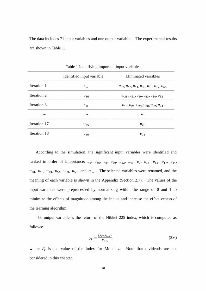
The data includes 71 input variables and one output variable. The experimental results
are shown in Table 1.
Table 1 Identifying important input variables
Identified input variable Eliminated variables
Iteration 1 𝜐6 𝜐37, 𝜐42, 𝜐41, 𝜐35, 𝜐48, 𝜐47, 𝜐65
Iteration 2 𝜐36 𝜐38, 𝜐51, 𝜐19, 𝜐43, 𝜐34, 𝜐32
Iteration 3 𝜐8 𝜐18, 𝜐21, 𝜐23, 𝜐20, 𝜐22, 𝜐24
⋯ ⋯ ⋯
Iteration 17 𝜐55 𝜐28
Iteration 18 𝜐56 𝜐11
According to the simulation, the significant input variables were identified and
ranked in order of importance: 𝜐6, 𝜐36, 𝜐8, 𝜐50, 𝜐52, 𝜐49, 𝜐7, 𝜐14, 𝜐12, 𝜐17, 𝜐44,
𝜐30, 𝜐10, 𝜐33, 𝜐54, 𝜐53, 𝜐55, and 𝜐56. The selected variables were renamed, and the
meaning of each variable is shown in the Appendix (Section 2.7). The values of the
input variables were preprocessed by normalizing within the range of 0 and 1 to
minimize the effects of magnitude among the inputs and increase the effectiveness of
the learning algorithm.
The output variable is the return of the Nikkei 225 index, which is computed as
follows:
𝑦𝑡 =(𝑃𝑡−𝑃𝑡−1)
𝑃𝑡−1, (2.6)
where 𝑃𝑡 is the value of the index for Month 𝑡 . Note that dividends are not
considered in this chapter.

17
Among the selected input variables, we find that some variables, e.g., T-bill rate,
has been proven effective and used frequently by previous studies. However, most
input variables have not been previously examined; therefore, we verify the predicted
effects of these variables in the following models. In addition, due to the lag
associated with the publication of macroeconomic indicators, we applied a one-month
time lag to certain data. We consider that using these variables in the forecasting
models is similar to real-world practice.
2.4 Back Propagation Neural Network Training
2.4.1 Theory of Back Propagation Algorithm
The BP algorithm is a widely applied classical learning algorithm for neural networks
[28, 56, 64]. In the BP algorithm, we enter the in-sample data, and then the algorithm
adjusts the weights and bias of the network by repeated training in such a way that the
error between the desired output and the actual output is reduced. When the error is
less than a specified value or when termination criteria are satisfied, training is
completed and the weights and bias of the network are saved.
Fig. 4 shows the illustration of an ANN processing unit, and the simple algorithm
steps of BP algorithm are shown as follows:
Step 1: Initialize the connection weights 𝑤𝑖𝑗, which is between i th neurons in the
previous layer and Unit j. Random the value of the biases 𝜃𝑗 for each
processing (hidden or output) Unit j.
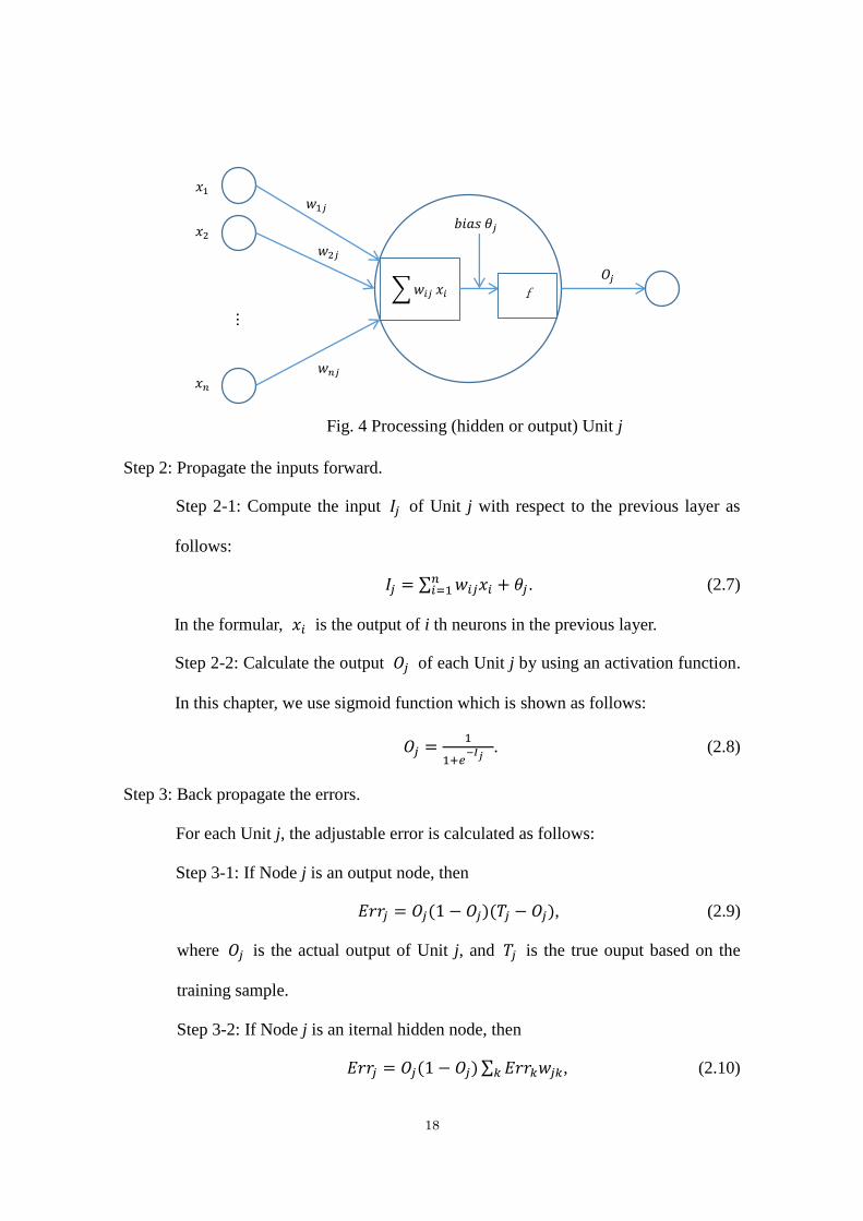
18
Step 2: Propagate the inputs forward.
Step 2-1: Compute the input 𝐼𝑗 of Unit j with respect to the previous layer as
follows:
𝐼𝑗 = ∑ 𝑤𝑖𝑗𝑥𝑖𝑛𝑖=1 + 𝜃𝑗 . (2.7)
In the formular, 𝑥𝑖 is the output of i th neurons in the previous layer.
Step 2-2: Calculate the output 𝑂𝑗 of each Unit j by using an activation function.
In this chapter, we use sigmoid function which is shown as follows:
𝑂𝑗 =1
1+𝑒−𝐼𝑗
. (2.8)
Step 3: Back propagate the errors.
For each Unit j, the adjustable error is calculated as follows:
Step 3-1: If Node j is an output node, then
𝐸𝑟𝑟𝑗 = 𝑂𝑗(1 − 𝑂𝑗)(𝑇𝑗 − 𝑂𝑗), (2.9)
where 𝑂𝑗 is the actual output of Unit j, and 𝑇𝑗 is the true ouput based on the
training sample.
Step 3-2: If Node j is an iternal hidden node, then
𝐸𝑟𝑟𝑗 = 𝑂𝑗(1 − 𝑂𝑗)∑ 𝐸𝑟𝑟𝑘𝑤𝑗𝑘𝑘 , (2.10)
𝑥1
𝑥2
𝑤𝑖𝑗 𝑥𝑖 f
𝑏𝑖𝑎𝑠 𝜃𝑗
𝑤1𝑗
𝑤2𝑗
𝑤𝑛𝑗
…
𝑥𝑛
𝑂𝑗
Fig. 4 Processing (hidden or output) Unit j

19
where 𝑤𝑗𝑘 is the connection weight from Unit j to Unit k in the next higher
layer, and 𝐸𝑟𝑟𝑘 is the error of Unit k.
Step 4: Update of the weights and biases.
Step 4-1: For each weight 𝑤𝑖𝑗 in the network,
Δ𝑤𝑖𝑗 = 𝑙 ∗ 𝐸𝑟𝑟𝑗𝑂𝑖, (2.11)
𝑤𝑖𝑗 = 𝑤𝑖𝑗 + Δ𝑤𝑖𝑗, (2.12)
where Δ𝑤𝑖𝑗 is the change in weight 𝑤𝑖𝑗. The variable 𝑙 is the learning rate,
a constant typically having a value between 0.0 and 1.0.
Step 4-2: For each bias 𝜃𝑗 in the network,
Δ𝜃𝑗 = 𝑙 ∗ 𝐸𝑟𝑟𝑗, (2.13)
𝜃𝑗 = 𝜃𝑗 + Δ𝜃𝑗 , (2.14)
where Δ𝜃𝑗 is the change in weight 𝜃𝑗 .
Step 5: Select the next pair of input patterns and then train the network repeatedly
according to Step 2. Training stops when: all Δ𝑤𝑖𝑗 in the previous epoch were
so small to below some specified threshold, or a prespecified number of epochs
has expired.
2.4.2 Numerical Experiment
We used the in-sample data described in Section 2.2.1 for training the numerical
experiments. To optimize the ANN learning algorithm, we conduct experiments of
parameter settings for the network using the BP algorithm to determine the most
appropriate parameters rather than choosing effective parameter values from a review of
domain experts and prior research. The ANN parameters and their levels are
summarized in Table 2. Ten levels of n, nine levels of mc, and ten levels of ep were

20
tested in the experiments. The larger the learning rate is, the greater is the adjustment
amounts. It is noted that, as suggested in the literature, a small value of l (0.1) was
selected. The momentum item of BP algorithm acts like a damper, which can restrain
oscillations and improve the convergence property [49]. The addition of momentum
stabilizes the descent path by preventing extreme changes in the gradient due to local
anomalies. We obtained a different mean square error (MSE) value for each iteration
when the ANN was trained by the same combination of parameters. Therefore, we ran
the experiment once for each parameter combination.
Table 2 Tested ANN parameters and levels
Parameter Meaning Level(s)
n The number of neurons in the hidden layer 10, 20, … 100
ep number of iterations 1000, 2000, … 10000
mc momentum constant 0.1, 0.2, … 0.9
l value of learning rate 0.1
The parameter setting experiments were performed with 900 parameter
combinations. We selected the parameter combination that resulted in the best
performance. Note that we used the MSE method to evaluate the performance of the
ANN model:
𝑀𝑆𝐸 =1
𝑁∑ (𝑦𝑡 − �̂�𝑡)
2𝑁𝑡=1 , (2.15)
where 𝑦𝑡 denotes the actual return of the Nikkei 225 index, and �̂�𝑡 is the predicted
return.
Among the 900 parameter combinations, we found that the most appropriate

21
parameter combination was n = 10, ep = 3000, mc = 0.4, and l = 0.1. The MSE value
of the best BP training algorithm for the ANN (i.e., BPNN) model was 0.0017. The
average MSE value obtained from the 900 training experiments was 0.1219.
During the experiment, we observed the following characteristics.
• Calculation time increased with an increased number of neurons in the hidden layer;
however, it was observed that the MSE value did not decrease gradually.
• Parameter combinations with relatively small MSE values always have relatively
fewer neurons in the hidden layer. Note that the MSE value is relatively small
when the number of neurons in the hidden layer ranges from 10–30.
• When the number of neurons in the hidden layer was large, the computer spent more
time capturing nonlinear relationships among the variables. However, for many
parameter combinations with a large number of neurons in the hidden layer, the
experiment terminated in a short period of time. We speculate that the experiments
achieved the best solution in the region of their starting point, which is the local
minimum.
• Due to the complex nature and large volume of data, the time required to achieve
convergence was significant; i.e., approximately one hour per parameter
combination.
2.5 Empirical Results
2.5.1 Linear Regression Model
In order to verify the effectiveness of the ANN model with BP algorithm, we

22
conducted linear regression model to compare with it. In this chapter, we used the
method of backwards for establishing the linear regression model. This method started
with the full set of input variables, and then removed the variable which had the least
contribution to the model from the last updated set. The final model was generated
until there cannot delete any variables which significantly affect the model. The
significant t-test was used as criteria of the significant input variables in the linear
regression model. The remaining variables were thus used to predict the stock market
returns. In this chapter we kept 𝑥2, 𝑥3, 𝑥8, 𝑥9, 𝑥13 and 𝑥15 as the significant input
variables in the regression model. The regression model has the following function:
𝑅𝑡 = 0.000000764 𝑥2 − 0.00003182 𝑥3 + 0.005506 𝑥8 + 0.004942 𝑥9
− 0.002047𝑥13 − 0.03664𝑥15 + 1.095 + 𝜀
Here 𝜀 is the error term, and follows the normal distribution. In this regression
model, all the regression coefficients are significant and the F-statistic is 3.388 (p-value
0.004<0.05), indicating that these forecasting variables can reflect the information of
the stock market returns. The regression model shows that the changes of 𝑥2, 𝑥8 and
𝑥9 have a positive effect on predictions of stock returns, whereas the effect of 𝑥3, 𝑥13
and 𝑥15 on stock market return is negative.
2.5.2 Numerical Results
In this chapter, the models were tested on Windows 7 operating system, and we
applied MATLAB R2011a by Math Works for operating all the experiments. Each of
the models described in the previous is estimated and validated by the in-sample data.
At this stage, the empirical evaluation for each model is based on the untouched

23
out-of-sample data which covers from January 2008 to July 2013 (67 months of
observations). This is due to the fact that the superior in-sample performance does not
always guarantee the validity of the forecasting accuracy.
With the formula of MSE above, the performance evaluation and the comparison of
different models are calculated in Table 3.
Table 3 Error analyses of different forecasting models.
Models LR BPNN best BPNN average level
MSE 12.7800 0.0044 0.1077
LR denotes the model of linear regression. Since 900 times of experiments on BP
traning had been executed in Section 2.4, here we chose the best (n=10, ep=3000,
mc=0.4, l=0.1) parameter combination of BPNN (Back propagation neural network)
model to compare with LR model. The average level of the performance of BP
algorithm is also shown in Table 3.
In the Table 3, the smaller the criteria is shown, the better is the prediction effect.
From Table 3, we can see that LR model has the largest value of MSE. The value of
MSE for the average level of BPNN model is 0.1077. The best model which we found
from the large number of experiments performs well and the value of MSE is 0.0044.
We conclude that the prediction ability of the BPNN model is much more effective than
the performance of the linear regression model. From the performance of the
experiments, we also find that even though the 18 effective input variables has not been
examined, the prediction effect is effective. The combination of 18 effective input
variables can be therefore a good alternative for stock market returns prediction.

24
2.6 Conclusion
In this chapter, in order to search more new effective input variables, which are used
to predict the return of Nikkei 225 index, we collected 71 variables that refer to different
aspects of the Japanese stock market. And then we selected new combination of input
variables of 18 good explanatory variables by fuzzy surfaces and utilized the
combination to predict the return. We used the monthly data of 18 good explanatory
variables to predict the return of Nikkei 225 index, and then compared the ability of the
prediction for different models. We found that the forecasting accuracy of ANN based
on BP algorithm was much more effective than the conventional linear regression. In
addition, the prediction effect of the combination of 18 input variables is effective, and
we may apply it for other stock markets for the future research.
2.7 Appendix: Input Variables
Input variables Meaning
𝑥1 Average Amounts Outstanding of Monetary Base
𝑥2 Banknotes in circulation of average amounts outstanding of monetary base
𝑥3 Coins in circulation of average amounts outstanding of monetary base
𝑥4 Uncollateralized overnight of call rates at the end of month
𝑥5 Yen spot rate at the end of month of Tokyo market
𝑥6 Yen central rate at the end of month of Tokyo market
𝑥7 Yen lowest in the month of Tokyo market
𝑥8 Percent changes from the previous year in average amounts outstanding of

25
money stock
𝑥9 Percentage changes in average amounts outstanding from the previous year of
loans and discounts for total of major and regional banks
𝑥10 Loans and discounts of regional banks
𝑥11 Import price index of all commodities
𝑥12 Real exports
𝑥13 Real imports
𝑥14 Indices of industrial production
𝑥15 1-year T-bill rate
𝑥16 2-year T-bill rate
𝑥17 3-year T-bill rate
𝑥18 4-year T-bill rate

26
Chapter 3 Improvement of Training Algorithms
3.1Introduction
In Chapter 2, we applied BP algorithm to train the neural network by conducting a
large number of experiments. The BP algorithm is a widely applied classical learning
algorithm for neural networks. Wong, Bodnovich and Selvi [65] found that most of
the studies that had used ANNs relied on gradient techniques for network training,
typically some variation of the BP algorithm. Although, researchers have commonly
trained ANNs using the gradient technique of the BP algorithm, limitations of gradient
search techniques emerge when ANNs are applied to complex nonlinear optimization
problems [53]. The BP algorithm has two significant drawbacks; i.e., slowness in
convergence and an inability to escape local optima [37]. In view of these limitations,
global search techniques, such as genetic algorithms (GA) and simulated annealing
(SA), have been proposed to overcome the local convergence problem for nonlinear
optimization problems.
This chapter attempt to determine the optimal set of initial weights and biases to
enhance the accuracy of ANN model by using GA and SA. The experimental results
show that hybrid approaches based on GA and SA improve the prediction accuracy of
the return of the Nikkei 225 index and outperform the BP training algorithm. In
addition, the effect on prediction of the combined 18 input variables is effective and can
therefore be a good alternative for predicting stock market returns.
The remainder of this chapter is organized as follows. Section 3.2 describes the
GA, and we apply the algorithm for improving the predictive ability of ANN model.

27
Then, we improve the ANN model by using SA in Section 3.3. Section 3.4 provides
the numerical experiments of ANN model improved by GA and SA. Finally, Section
3.5 contains the discussion and conclusion.
3.2 Improvement Using Genetic Algorithms (GA)
As observed in the parameter setting experiments, we find that the BP algorithm has
two drawbacks; i.e., trapping into local minima and slow convergence. Note that these
drawbacks have been verified by previous studies. To overcome these problems, many
studies prefer to utilize optimal global search techniques rather than gradient search
techniques such as the BP algorithm, which is designed for local search. Many studies
have used GA-based hybrid models to overcome the drawbacks of the BP approach [32,
43, 46]. The results of these studies support the notion that GA can enhance the
accuracy of ANN models and can reduce the time required for experiments [27].
Chang and Lin [26] proposed an auto-tuning method for the fuzzy neural network
by GA, and showed that the characteristic of the proposed system was to obtain the
minimal and the optimal structure of a fuzzy model. Marwan and Mat [6] used GA to
find the optimal set of initial weights to enhance the accuracy of artifical neural
networks. And their study of using simple GA has been proved to be effective for
improving the prediction accuracy of ANN. Subhra and Jehadeesan [48] compared
standard BP algorithm with GA based on BP algorithm on the prediction of parameters
in Nuclear Reactor Sbusystems. The experimental results showed that GA based
neural network saved a lot of time for the less number of iterations and faster
convergence than BP algorithm. In this chapter, GA algorithm is utilized to optimize
the initial weights and bias of the ANN model. Then, the ANN model is trained by the

28
BP algorithm using the determined weights and bias.
We encoded all the weights and bias in a string and generated the initial population.
Each solution generated by GA is referred to as a chromosome (or individual) [27].
The collection of chromosomes is called a population. Here, each chromosome
represents an ANN with a certain set of weights and bias. We evaluated each
chromosome of the population using a fitness function that is based on MSE.
Chromosomes with higher fitness values participate in reproduction and yield new
strings by the GA (e.g., crossover and mutation). Thus, we obtain a new population.
Through iterative progression, and after many generations, the population with the best
fitness values can be found.
Fig. 5 Process of the hybrid GA and BP algorithm
Fig.5 shows the procedure of the hybrid GA and BP algorithm. The algorithm
operated in this chapter consists of the following steps:
Step 1: Because of the wide range of the data, we normalized it to make sure that the
value of all the variables scale down between zero to one. We normalized the

29
variables as follows:
𝑅𝑁 =𝑅−𝑅𝑚𝑖𝑛
𝑅𝑚𝑎𝑥−𝑅𝑚𝑖𝑛, (3.1)
where R is a sample variable. RN is the normalized value of R, 𝑅𝑚𝑖𝑛 is the
minimum value of R, 𝑅𝑚𝑎𝑥 is the maximum value of R.
Step 2: Encode all the weights and bias in a string and generate the initial population.
Each solution generated in GA is called a chromosome (or an individual). The
collection of chromosomes is called a population. Here each chromosome
represent ANN with the certain set of wights and bias [37].
Step 3: Train the ANN model with BP algorithm, and then evaluate each chromosome
(individual) of the current population by a fitness function based on the MSE
value. The value of the fitness function is inversely proportional to the error.
Step 4: Rank all the individuals by the fitness proportion method, and then select the
individuals with the higher fitness value to pass on to the next generation
directly.
Step 5: Apply the genetic algorithms (e.g., crossover, mutation) to current population
and then creat new chromosomes. Evaluate the fitness value of the new
chromosomes, and insert the new chromosomes into the population to replace
worse individuals of the current population. And then we get the new
population.
Step 6: Repeat the Steps 3-5 until stopping conditions reach.

30
3.3 Improvement Using Simulated Annealing (SA)
SA, which is first presented by Kirkpatrick, Gelatt and Vecchi [33], is a famous
optimization method that can be widely and successfully employed in solving global
optimization problems in many research fields. The major advantage of SA is that it
accepts both better and worse neighboring solutions that have a certain probability so as
to jump out of a local optimum to search for the global optimum [55]. Many prior
studies have successfully applied the SA algorithm to optimize the structure of an ANN
model in various applications [1, 59, 66].
Yamazaki, De Souto and Ludermir [66] applied SA to the optimization of neural
network weights and architectures. Their work showed that SA algorithm was able to
produce networks with low complexity and better generalizaion performance than
network trained with the BP algorithm for the odor classification task. Abbasi and
Mahlooji [1] used ANN to estimate a response surface and applied SA to find the
optimal or near optimal response. The results indicated that the proposed algorithm
outperformed the classical method. Sudhakaran and Sivasakthivel [59] utilized a
feed-forward BP network to predict the depth of penetration. Their work also proved
the success of using SA in searching the optimum values of the process variables of
penetration for stainless steel gas tungsten arc welded plates.
In this chapter, the SA technique is used to optimize the weights and bias of a
BP-trained ANN model. The implementation of the SA algorithm is remarkably easier
than the GA algorithm, and the process of hybrid SA and BP algorithm is shown in
Fig.6.

31
Fig. 6 Process of the hybrid SA and BP algorithm
The basic structure of SA algorithm is presented as follows:
Step 1: Normalize all the data to the range [0,1]. Initialize the SA control parameter 𝑇0
and temperature reduction value.
Step 2: Set 𝑆0 (the elements of 𝑆0 are all the weights and biases of ANN model) as the
initial solution. For all the training sample, we calculate the predicted output
value of ANN which is trained with the BP algorithm. The sum of squared errors
𝐸0 is calculated by the error between the predicted value and the real value.
Step 3: A new candidate solution 𝑆1 is generated by means of small random
perturbation ∆S of the current solution 𝑆0, 𝑆1 = 𝑆0 + ∆S.
Step 4: Calculate the sum of squared errors 𝐸1 based on the new candidate 𝑆1.
Step 5: If 𝐸1 < 𝐸0, we accept 𝑆1 as the current solution.
else we accept 𝑆1 as the current solution with the probability
P = 𝑒𝑥𝑝(−(𝐸1−𝐸0)
𝑇𝑖), (3.2)
where 𝑇𝑖 is the current temperature.

32
Step 6: Repeat Step 3 – Step 5 until the system reaches steady state or thermal
equilibrium.
Step 7: Drop the temperture T according to the given temperature reduction strategy,
and repeat Step 3 – Step 6 until T=0 or certain low temperature value 𝑇𝐿.
In SA, we started the algorithm with a relatively high value of T , to avoid being
prematurely trapped in a local optimum. The most important feature of this algorithm
is presented in Step 5, which is the possibility of accepting a worse solution, hence
allowing it to prevent falling into a local optimum trap. There are two loops in the
algorithm: in the outer loop the temperature is changed and the linner loop determines
how many neighbourhood can be attempted at each temperature. The algorithm
proceeds by attempting a certain number of neighbourhood moves at each temperature,
while the temperature parameter is gradually dropped [12].
3.4 Numerical Results
Because of the superior in-sample performance did not always guarantee validity of
forecasting accuracy, here the empirical evaluation of each model was based on the
untouched out-of-sample data (January 2008 to July 2013; 67 months of observations).
The MSE and CPU time (for training and prediction) results of the performance
evaluations for each algorithm are shown in Table 4. The models were tested by using
the Windows 7 operating system. In addition, MathWorks MATLAB R2011a was
employed in all experiments.

33
Table 4 Error analyses of different forecasting models
Models BPNN
best
BPNN
average
GABPNN
best
GABPNN
average
SABPNN
best
SABPNN
average
MSE 0.0044 0.1077 0.0043 0.0090 0.0725 0.0862
CPU
Time*
68 1080 1322 28 40
* CPU Time for a 2.66 GHz Intel Core 2 Duo E6750
Nine hundred BP training experiments were executed, and we selected the best
combination of parameters (n = 10, ep = 3000, mc = 0.4, l = 0.1) for the BPNN model as
a baseline for comparison with the other models. The average performance of the BP
algorithm is also shown in Table 4. Note that GABPNN denotes the hybrid GA and
BP training algorithm used in the neural network. The cross probability and mutation
probability values of the experiments were changed 81 times. This resulted in the best
and average performances of the GABPNN model. SABPNN is a hybrid SA and BP
training algorithm. The SABPNN experiments were performed 10 times, and the
temperature of each experiment was 100. The best and average ability of the
SABPNN to estimate stock returns are also shown in Table 4.
Here, we exclude computing time and give a simple comparison of the error
indicator values. Note that smaller criterion values indicate better prediction effects.
Compared to the BPNN average, GABPNN and SABPNN overcome the local
minimum weakness and greatly improve prediction accuracy. SABPNN models with
lower MSE values are superior to the average level of the BPNN experiments, especially
for the hybrid GA and BP approach. Note that the MSE value of the best model is

34
0.0043. Compared to the BPNN average, the average MSE of the GABPNN model is
also effective, demonstrating a value of 0.0090. The best BPNN model also
demonstrate effective performance with an MSE value of 0.0044.
In terms of running time for the three models, the BPNN models may demonstrate
the shortest time because they easily fall into the local minimum with bad performance.
If not, the time requires to reach convergence is very long; i.e., approximately one hour
for each parameter combination with a large number of hidden neurons. There is no
sense to provide the average CPU time for the BPNN. Computing time is 68 seconds
when the best BPNN model is not caught in the local minimum. Although the running
time of the best BPNN is short, excessive time is required to search for the most
appropriate parameter combination for the BPNN models. The SABPNN requires
only 28 seconds, which helps the BP algorithm jump out of the local search. The
average time for the SABPNN is less than the other models. The GABPNN requires
longer time than the SABPNN; 18 minutes of run time is required, but it reduces the
MSE value significantly.
The run time of the SABPNN is faster than any other models, and the prediction
accuracy is higher than the normal BP model levels. By synthesizing the performances
of the accuracy of prediction and the running time of the experiments, we consider that
GABPNN demonstrates better market return prediction performance and higher
accuracy than the other models.
Chen et al. [8] applied BP neural networks and Support Vector Machines (SVM) to
construct the prediction models for forecasting the six major Asian stock market indices.
They followed the previous research and determined the five input variables that were
transformed from the daily closing price. They applied the ANN model with BP

35
algorithm to the six Asian markets and the value of MSE for Nikkei 225 index was
0.048. Dai et al. [10] proposed a time series prediction model (NLICA-BPN model)
by combining nonlinear independent component analysis and neural network to forecast
Asian stock markets. Their experimental results showed that the forecasting model
could produce lower prediction error and improve the prediction accuracy of the neural
network approach with the value of RMSE for Nikkei 225 was 50.44. Lu [28] applied
an integrated independent component analysis based denoising scheme with neural
network in stock price prediction. Four forecasting variables were used for predicting
the Nikkei 225 index, including the previous day’s cash market closing index and three
Nikkei 225 index futures. The empirical results showed that the proposed ICA-BPN
method performed well in forecasting the Nikkei 225 index and the value of RMSE was
43.54.
Compared with the prior research and according to the experimental results, we find
that even though most of the proposed 18 input variables have not been used in previous
studies, their effect on prediction is remarkable. Thus, these input variables are
considered a good choice for prediction of stock market returns. The optimization
afforded by the GA or SA has demonstrated strong potential for obtaining globally
optimal solutions. The GA can quickly achieve the best prediction accuracy for the
ANN model while the BP algorithm requires to test a large number of parameter
combinations.

36
3.5 Conclusion
In this chapter, we applied GA and SA for improving the accuracy of ANN model
with BP algorithm. In the light of significant drawbacks of BP algorithm, we proposed
to use global search techniques, such as GA and SA, to optimize the weights and bias of
the ANN. The experimental results showed that hybrid approach of SA and BP
overcame the weakness of local minima and greatly improved prediction accuracy. We
synthesized the performance of the prediction accuracy and running time, and
considered that the hybrid GA and BP approach provided higher accurate forecasting of
future values than other prediction models. In addition, the effect on prediction of the
combined 18 input variables was effective and can therefore be a good alternative for
predicting stock market returns.

37
Chapter 4 Predicting the Direction of Stock Price
Index Movement
4.1 Introduction
In this chapter, we predict the direction of the daily Nikkei 225 index by using ANN
with genetic algorithm (GA).
It is a difficult task to predict the exact value of a stock market index, hence there
are many researches that are concerned with the prediction of the direction of stock
price index movement. The direction of the stock market index is the sign of price
index or the trend of the stock market index in the future. Mark and Leung [38] hold
the view that trading could be profitable by an accurate prediction of the direction of
movement. Their work suggested that financial forecasters and traders should be focus
on accurately predicting the direction of movement so as to minimize the estimates’
deviations from the actual observed values. Mostafa [44] also believed that accurate
predictions of the direction of stock price indices were very important for investors.
Previous studies have applied various models in forecasting the direction of the stock
market index movement. Huang et al. [25] forecasted stock market movement by
support vector machine (SVM), and concluded that the model was good at predicting
the direction. Kara et al. [29] applied artificial neural networks (ANN) and SVM in
predicting direction of the Istanbul Stock Exchange. Their study proves that the two
different models are both useful prediction tools, and ANN is significantly better than
the SVM model. In addition, scholars predict the movement of the stock market
indices of various countries. Leung et al. [38] forecasted the direction of the return for

38
three globally traded broad market indices, S&P for the US, FTSE 100 for the UK and
Nikkei 225 for Japan by various models. Their research shows that the classification
models perform better than the level estimation counterparts in terms of the number of
times the predicted direction is correct. Senol and Ozturan [54] applied seven
different prediction system models for predicting the direction of the stock market index
in Turkey, and concluded that ANN could be useful in forecasting. The main
contribution of this chapter is that we predict the direction of the next day’s price of the
Nikkei 225 index by using the GA-ANN hybrid model.
The forecasting of financial index is characterized by data intensity, noise,
non-stationary, unstructured nature, high degree of uncertainty, and hidden relationships
[21, 30, 60]. Many factors, such as political events, general economic conditions, and
traders’ expectations, may have influence on the price of stock market. Many
researches use similar indicators to forecast the stock market index. The core objective
of this chapter is to compare two basic types of input variables to predict the direction
of the daily Nikkei 225 index by using ANN model with GA algorithm. In this chapter,
we demonstrate and verify the predictability of stock price direction by using ANN with
GA, and then compare the performance with prior studies. Empirical results shows
that input variables Type 2 can generate higher forecast accuracy.
The remainder of this chapter is organized as follows. Section 4.2 describes the
data, and input variables that are used in the ANN model. Then, we show the
procedure of predicting the stock market direction in Section 4.3. Section 4.4 provides
the experimental results of two types of indicators, and compares the results with
similar studies. Finally, Section 4.5 contains the discussion and conclusion.
Formulas and the summary statistics for each feature of input variables are given in

39
Section 4.6.
4.2 Research Data
4.2.1 Data
The research data used in this chapter are technical and fundamental indicators
which are calculated by the daily price of the Nikkei 225 index. The total number of
samples is 1707 trading days, from January 2007 to December 2013. The total 1707
data points of the daily Nikkei 225 closing cash prices in the data set are shown in Fig. 7.
We divide the entire data into two parts, 78.6% of the data is used for in-sample training
and 21.4% for out-of-sample data. The in-sample data is used to determine the
specifications of the model and parameters while the out-of-sample data is reserved for
the evaluation of model. The financial data used in this chapter is obtained from the
Yahoo Finance.
In the light of previous studies, it is hypothesized that various technical indicators
may be used as input variables in the construction of prediction models to forecast the
direction of movement of the stock price index [51]. Tables 5 and 7 give selected
features and their formulas, and we select technical indicators as feature subsets by the
review of prior researches [2, 24, 54].
The original data are standardized before being applied to the ANN experiments. We
normalize the data as follows,
𝑋𝑁 =𝑋−𝑋𝑚𝑖𝑛
𝑋𝑚𝑎𝑥−𝑋𝑚𝑖𝑛, (4.1)
where X is a data point. XN is the normalized value of X, 𝑋𝑚𝑖𝑛 is the minimum value

40
of X, 𝑋𝑚𝑎𝑥 is the maximum value of X. The goal of linear scaling is to independently
normalize each feature component to the specified range. It also ensures that the larger
value input attributes do not overwhelm smaller value inputs, and helps to reduce
prediction errors [31].
Fig. 7 The daily Nikkei 225 closing prices from January 23, 2007 to December 30, 2013
4.2.2 Input Variables
In this chapter, we want to compare the performances of two sets of input variables.
From the prior studies we notice that, most of scholars want to choose the input
variables as shown in Table 5, meanwhile others want to use the variables in Table 6.
In this chapter, we conduct the experiments by using ANN model with the two types of
input variables, and then compare the performance of these two experiments with prior
studies.
0
2000
4000
6000
8000
10000
12000
14000
16000
18000
20000
2007/1/23 2008/1/23 2009/1/23 2010/1/23 2011/1/23 2012/1/23 2013/1/23
Clo
sin
g
Pri
ce

41
4.2.2.1 Input Variables Type 1
We set 13 technical indicators as Type 1 feature subset by the prior researches [29,
32]. Table 5 shows these indicators, their formulas and the summary statistics for each
feature of Type 1 are presented in the appendix.
Table 5 Selected technical indicators and their formulas (Type 1)
Name of feature Formulas
Stochastic %K (𝐶𝑡 − 𝐿𝑛)/( 𝐻𝑛 − 𝐿𝑛)×100,
Stochastic %D ∑ %𝐾𝑡−𝑖𝑛−1𝑖=0 /𝑛,
Stochastic slow %D ∑ %𝐷𝑡−𝑖𝑛−1𝑖=0 /𝑛,
Momentum 𝐶𝑡 − 𝐶𝑡−4,
ROC (rate of change) 𝐶𝑡/𝐶(𝑡−𝑛) × 100,
LW%R (Larry William’s %R) (𝐻𝑛 − 𝐶𝑡)/( 𝐻𝑛 − 𝐿𝑛)×100,
A/O Oscillator (accumulation/distribution
oscillator)
(𝐻𝑡 − 𝐶𝑡−1)/( 𝐻𝑡 − 𝐿𝑡),
Disparity 5 days 𝐶𝑡/𝑀𝐴5 × 100,
Disparity 10 days 𝐶𝑡/𝑀𝐴10 × 100,
OSCP (price oscillator) 𝑀𝐴5 −𝑀𝐴10/𝑀𝐴5,
CCI (commodity channel index) (𝑀𝑡 − 𝑆𝑀𝑡)/(0.015 × 𝐷𝑡),
RSI (relative strength index) 100 − 100/(1 +∑ 𝑈𝑝𝑡−𝑖𝑛−1𝑖=0
n/∑ 𝐷𝑤𝑡−𝑖𝑛−1𝑖=0
n),
where 𝐶𝑡 is the closing price of the Nikkei 225 index at time t,
𝐿𝑡 is the low price of the Nikkei 225 index at tme t,

42
𝐿𝑛 is the lowest low price of the Nikkei 225 index in the last n days,
𝐻𝑡 is the high price of the Nikkei 225 index at time t,
𝐻𝑛 is the highest high price of the Nikkei 225 index in the last n days,
𝑀𝐴𝑛 is the moving average of price in the last n days,
𝑀𝐴n = (∑ 𝐶𝑡−𝑖+1𝑛𝑖=1 )/𝑛, (4.2)
𝑀𝑡 =𝐻𝑡+𝐿𝑡+𝐶𝑡
3, (4.3)
𝑆𝑀𝑡 = (∑ 𝑀𝑡−𝑖+1𝑛𝑖=1 )/𝑛, (4.4)
𝐷𝑡 = (∑ |𝑀𝑡−𝑖+1𝑛𝑖=1 − 𝑆𝑀𝑡|)/𝑛, (4.5)
𝑈𝑝𝑡 is the upward price change of the Nikkei 225 index at time t,
𝐷𝑤𝑡 is the downward price change of the Nikkei 225 index at time t.
4.2.2.2 Input Variables Type 2
We set 9 technical indicators as Type 2 feature subset from the prior researches [54,
60]. Table 6 shows these indicators, the definitions and the summary statistics for each
feature of Type 2 are presented in the appendix.

43
Table 6 Selected technical indicators’ formulas (Type 2)
Name of indicator Formulas
OBV 𝑂𝐵𝑉𝑡 = 𝑂𝐵𝑉𝑡−1 + Ɵ ∗ 𝑉𝑡,
𝑀𝐴5 𝑀𝐴5 = (∑ 𝐶𝑡−𝑖+15𝑖=1 )/5,
BIAS6 BIAS6 = (𝐶𝑡−𝑀𝐴6
𝑀𝐴6) × 100%,
𝑃𝑆𝑌12 𝑃𝑆𝑌12 = (𝐴/12) × 100%,
𝐴𝑆𝑌5 𝐴𝑆𝑌5 = (∑ 𝑆𝑌𝑡−𝑖+15𝑖=1 )/5,
𝐴𝑆𝑌4 𝐴𝑆𝑌4 = (∑ 𝑆𝑌𝑡−𝑖+14𝑖=1 )/4,
𝐴𝑆𝑌3 𝐴𝑆𝑌3 = (∑ 𝑆𝑌𝑡−𝑖+13𝑖=1 )/3,
𝐴𝑆𝑌2 𝐴𝑆𝑌2 = (∑ 𝑆𝑌𝑡−𝑖+12𝑖=1 )/2,
𝐴𝑆𝑌1 𝐴𝑆𝑌1 = 𝑆𝑌𝑡−1,
where 𝑉𝑡 is the volume of trade of the Nikkei 225 index at time t,
Ɵ = {+1, 𝐶𝑡 ≥ 𝐶𝑡−1 −1, 𝐶𝑡 < 𝐶𝑡−1
, (4.6)
Ɵ is positive when the closing price is above the prior closing price, and Ɵ is negative
when the closing price is below the prior close.
4.3 Prediction Process
As we have mentioned the algorithms of BP, GA and SA in the last two chapters,
empirical results show that the GA-ANN hybrid model has the most effective predictive
ability. In this chapter, we propose to apply the GA algorithm to optimize the weights
and bias of ANN model, and then predict the direction of daily closing price movement

44
of Nikkei 225 index.
The architecture of our experimental process is shown in Fig. 8. First we calculate
all the data of two types of input variables. Then we standardize the data to reduce the
experiments’ errors. We apply two types of indicators for predicting the direction of
next day’s movement by the GA-ANN hybrid model respectively. After we finish all
the experiments, we compare the performance among the two types of input variable set
and prior studies.
Fig. 8 Architecture of the experimental process for comparing two types of input
variables
4.4 Experimental Results
4.4.1 Comparison of the Performances between the Two Types of Input Variables
In the period of training the GA-ANN hybrid model, we use the in-sample data.
Then we test the performance of the two sets input variables by applying out-of-sample
data which includes 300 data points. Table 7 shows the performances of the two types
of input variables. Hit ratio denotes the ratio when the predicted direction is correct.
The hit ratio for forecasting the direction of next day’s price correctly by applying input
variables Type 1 is 60.87%, and 81.27% by input variables Type 2. We can conclude

45
that input variable Type 2 is more effective in predicting the direction of daily closing
price of Nikkei 225 index than input variable Type 1.
Table 7 The comparison between two types of input variables
Type 1 Type 2
Hit ratio (%) 60.87 81.27
According to Fig. 9, we can find that the good performance obtained by input
variable Type 2, and the direction of real value line is as similar as the predicted one.
The probability of the prediction for the direction of the next day’s closing price is
81.27%. We infer that the accurate prediction performance of the ANN model by
using input variables Type 2 is useful for investors and can become a good candidate for
predicting the direction of next day’s closing price.
Fig. 9 Performance of the predicted closing price by applying input variables Type 2
0
5000
10000
15000
20000
1
11
21
31
41
51
61
71
81
91
101
111
121
131
141
151
161
171
181
191
201
211
221
231
241
251
261
271
281
291
closing price predicted closing price

46
4.4.2 Comparison of Results with Similar Studies
Predicting the direction of the stock market index is an important topic for the
investors. Accurate prediction of stock prices movement may generate attractive
benefits for investors. There are many studies that are focus on the prediction of
movements. Table 8 shows the prior studies that are aim to predict the direction of
stock market indices by various methods. The result of this chapter is also compared
with these researches in Table 8.
Table 8 Comparison of our study with prior papers
Studies Methods Stock market Hit ratio (%)
Kim and Han [32] GA feature discretization Korea 61.70
Leung et al. [38] Classification model US, UK, Japan 68 (Nikkei 225)
Huang et al. [25] SVM Japan 75
Kara et al. [29] BPNN Istanbul 75.74
Our study GA-ANN hybrid model Japan 81.27
According to the table, we find that the performances are significantly different in
various stock markets, and our model is superior to other models. Thus, we consider
that the set of input indicators and GA algorithm adopted in this chapter can be
considered as more appropriate for prediction.

47
4.5 Conclusion
In this chapter, we tried to apply two types of technical indicators to predict the
direction of next day’s Nikkei 225 index movement. We adjusted the weights and bias
of ANN model by GA algorithm, then we tested the performance of the GA-ANN
hybrid model by applying two types of input variables. The experiments implied that
input variables Type 2 can generate higher performance, and the probability for
predicting the direction was 81.27%. We also compared the performance of the
GA-ANN hybrid model with similar studies, the results showed that our method was
more effective and can generate higher prediction accuracy.
However, the prediction performance of this chapter can be improved by two ways.
The first way is to combine the two types of input indicators, or test some subset of
these variables. In addition, we can add some other macroeconomic variables such as
variables showed in Chapter 2. Second, not only GA algorithm, other optimal methods
can be used to adjust the parameters of ANN model. We can even use other models,
such as probabilistic neural network for predicting the movement of Nikkei 225 index.
These two improvements can be a future work for our study.
4.6 Appendix: Description of the Input Variables
In this appendix, we describe two types of input variables which are applied to
forecast the direction of Nikkei 225 index.
The descriptive statistics for Type 1 input variable is shown in Table 9. Stochastic
Oscillator is an indicator that is used for predicting price turning points by comparing

48
the closing price of a security with its price range. It includes K line and D line.
Table 9 The summary of statistics (Type 1)
Name of feature Max Min Average Standard deviation
Stochastic %K 100.000 0.000 53.302 33.525
Stochastic %D 98.731 1.450 53.287 27.594
Stochastic
slow %D
98.229 2.121 53.269 25.485
Momentum 1492.680 −2196.660 −2.319 366.566
ROC 119.742 76.969 100.041 3.281
LW%R 100.000 0.000 46.698 33.525
A/O Oscillator 4.483 −2.919 0.577 0.936
Disparity 5 days 113.795 86.815 99.999 1.819
Disparity 10 days 113.316 79.788 99.998 2.690
OSCP 0.067 −0.097 0.000 0.015
CCI 166.667 −166.667 5.408 93.381
RSI 99.875 0.000 51.831 18.234
The descriptive statistics for Type 2 input variable is summarized in Table 10. On
Balance Volume (OBV) measures buying and selling pressure as a cumulative indicator
that adds volume on up days and subtracts volume on down days. It is also an
indicators for measuring positive and negative volume flow. A rising OBV reflects
positive volume pressure that can lead to higher prices. Conversely, falling OBV
means that negative volume pressure can foreshadow lower prices [19].

49
BIAS𝑛 measures the divergence of current stock price from an n day simple moving
average of the stock prices. Normally scholars and investors choose n to be 6 days.
The value of BIAS𝑛 may be above or below the moving average when the closing price
is far away from the average level.
𝑃𝑆𝑌n is the Psychological line, which is a sentiment indicator, and it is made to look
behind the obvious mood of the market and to detect undertones for a tend change.
𝑃𝑆𝑌n is the ratio of the number of rising periods over the n days period. A is number
of the rising days in the last n days.
𝑆𝑌𝑡 is the return of the Nikkei 225 index at time t, 𝑆𝑌𝑡 = (ln 𝐶𝑡 − ln 𝐶𝑡−1) × 100.
𝐴𝑆𝑌𝑛 is the average return in the last n days.
Table 10 The summary of statistics (Type 2)
Name of feature Max Min Average Standard deviation
OBV 1769930.000 −1188269.000 255381.867 340334.874
𝑀𝐴5 18209.158 7177.696 11507.384 2947.335
BIAS6 18199.282 7211.380 11504.454 2944.715
𝑃𝑆𝑌12 0.126 -0.147 0.000 0.020
𝐴𝑆𝑌5 0.917 0.000 0.514 0.132
𝐴𝑆𝑌4 0.048 -0.056 0.000 0.007
𝐴𝑆𝑌3 0.045 -0.065 0.000 0.008
𝐴𝑆𝑌2 0.077 -0.068 0.000 0.010
𝐴𝑆𝑌1 0.085 -0.088 0.000 0.012

50
Chapter 5 Dogs of the Dow Investment Strategy
5.1 Introduction
In the stock market, one of the aims of investors is to “beat the market,” i.e., to
outperform benchmarks such as the Dow Jones Industrial Average or Nikkei Average.
This aim, however, is not easily achieved even by professional fund managers. For
example, a study on the American funds reported that 75% of them underperformed
benchmarks [13], and the situation for the Japanese fund managers is even worse. As
for individual investors, most of them lack advanced professional skills or do not have
enough time to study the stock market. As a consequence, most of them are losers in
the market. Therefore, effective investment strategies, which should be simple and
easy-to-practice, are necessary for both professional and individual investors.
Investments in stock market have always been built around some kind of
investment philosophy or strategy, some naïve, others more complex. While some
investment strategies have paid off, others have not proved as effective [52].
Nevertheless, considerable research continues to be made in searching of effective
strategies, scholars and investors continue to yearn for new strategies to beat the market
and achieve abnormal returns out of investments made in the stock market. Among
many effective strategies which have been tested in recent years, one strategy which has
gained great popularity in the investment community and has been studied extensively
by academia. The strategy was first proposed by analyst John Slatter, and the article
was published in a Wall Street Journal. This strategy involves investing equal amounts
in the 10 highest-yielding stocks of the Dow Jones Industrial Average (DIJA) index at

51
the end of the year, and then holding these high-yielding stocks for 1 year [11].
According to the effective performance of these highest-yielding stocks, which was
proved by investors, these stocks tend to be called “Dog” stocks. Therefore, Slatter’s
investment strategy is commonly referred to as the “Dogs of the Dow” strategy. This
strategy, also known as the Dow 10 strategy, is a very popular and successful investment
strategy in the United States. Slatter examined the performance of the Dogs of the
Dow strategy for the years 1973 through 1988, and found that the 10
highest-dividend-yielding stocks of DJIA outperformed DJIA.
Since then, many papers have been written on the American stock market.
O’Higgins and Downes [47] and Knowles and Petty [34] published books examining
the performance of the Dogs of the Dow strategy over longer time horizons. These
studies show the effectiveness of this strategy from 1973 to 1991. While these books
increased the popularity of the strategy, they also raised new concerns. Nonetheless,
they attracted more investors and scholars to apply the strategy. The first academic
study on the Dogs of the Dow strategy was performed by McQueen et al. [42]. They
used statistical methods to examine the performance of the portfolio over 50 years
(1946–1995), and concluded that this strategy’s superiority is statistically significant.
Encouraged by its success in the United States, scholars in many countries have
examined the strategy [9, 18]. Visscher and Filbeck [63] showed that the Dogs of the
Dow strategy performed well against the Toronto 35 and TSE 300 indices in the
Canadian stock market. The strategy was also widely examined in Latin American and
Polish stock markets. Furthermore, Eemeli and Sami [50] concluded that the Dogs of
the Dow strategy can be successfully applied to the Finnish stock market. In Japan,
Song and Hagio [57] proposed the application of this strategy to the Tokyo Stock

52
Exchange, and concluded that it performed well when it was applied in NIKKEI 225 for
the 2002–2006 data.
Our purpose is to analyze the performance of the Dogs of the Dow strategy in the
Japanese stock market for a longer term and the Hong Kong stock market in order to
examine its validity.
For the Japanese stock market, first we conduct a simulation using the 1981–2010
data and compare the performance of the Dogs of the Dow strategy with that of
NIKKEI 225 index. The results show that the strategy outperforms the index
remarkably. This provides empirical evidence for the effective application of the
strategy in the Japanese market. Second, because of the higher standard deviation of
the Dogs of the Dow strategy, we make risk adjustments by using the Sharpe Ratio,
drawing the comparison one more time. The results after adjusting for risk and
transaction costs make the strategy more convincing and rigorous. Third, this study
explores various versions of the Dogs of the Dow strategy, which provide more
implications for investors of the Japanese stock market.
For Hong Kong stock market, we conduct a simulation for the 2001–2011 data and
compare the performance of Dogs of the Dow strategy with that of the market index.
Further, in addition to the most popular version of the Dogs of the Dow strategy, which
uses the 10 highest-dividend-yielding stocks, we also test less well-known version of
the strategy which involves fewer Dogs.
This chapter is organized as follows: in Section 5.2, we show the simulation results
of Dogs of the Dow strategy in Japanese stock market. In the Section 5.3, we apply
Dogs of the Dow strategy to the Hong Kong stock market. Then we make a summary
in Section 5.4.

53
5.2 The Application for the Japanese Stock Market
5.2.1The Simulation
NIKKEI 225 (also known as NIKKEI average or the NIKKEI) is the most widely
used market index for the Tokyo Stock Exchange. It includes 225 stocks, which are
weighted equally, and has been calculated daily since 1950.
We implemented the simulation of the Dogs of the Dow investment strategy in three
steps. In step 1, we collected data for all 225 companies of NIKKEI 225 on March 31,
and then selected the 10 highest-dividend-yielding stocks. On April 1, we invested in
the 10 stocks with equal weighting. In step 2, we held these stocks for one year and
then sold them at the end of March of the following year. After updating the list of
NIKKEI 225, we invested in the new top-10 stocks with equal weighting on April 1.
In step 3, we repeated the process for each year.
We searched for the stock prices on the internet and in newspapers and obtained the
expected dividend price data of 225 companies of NIKKEI 225 from [61]. April 1 was
chosen as the investing date because it is the beginning of the fiscal year for most
Japanese companies.
In this section, we implemented the simulation for the 1981–2010 data.
5.2.2 Comparison of Dogs of the Dow Strategy and NIKKEI 225
Table 11 presents the average returns and standard deviations of the Dogs of the
Dow strategy and NIKKEI 225. The Dogs of the Dow strategy had an average return
of 13.61% and a standard deviation of 32.27%. The NIKKEI 225 portfolio had a

54
lower mean return and deviation at 3.97% and 24.17%, respectively. The table also
provides data on the difference between the two strategies. The Dogs of the Dow
strategy had a 9.64 percentage points higher return on average and the difference of the
standard deviation was 8.10 points. The data show that in the last 30 years, the Dogs
of the Dow strategy outperformed NIKKEI 225 on average, although the former had a
higher risk.
Table11 The annual return summary of statistics for the Japanese stock market
(1981-2010)
Portfolio Average annual return Standard deviation
Dogs of the Dow 13.61% 32.27%
NIKKEI 225 3.97% 24.17%
difference 9.64% 8.10%
To check the statistical significance of the result, we conducted a T-test at a 5%
significant level. In the test, p = 0.022705 < 0.05, and thus the higher performance is
statistically significant at a 95% confidence level.
Fig. 10 plots the differences between the Dogs of the Dow strategy and NIKKEI
225 annual portfolio returns for each year. Here, a positive difference indicates that
the Dogs of the Dow strategy outperformed the NIKKEI 225 portfolio.

55
Fig. 10 Annual difference in returns between the Dogs of the Dow strategy and NIKKEI
225
Fig. 10 indicates that the Dogs of the Dow strategy outperformed NIKKEI 225 on
21 occasions. Especially in 1985, the Dogs of the Dow strategy was 57.82 percentage
points greater than NIKKEI 225. In 2000, the Dogs of the Dow strategy was 50.30
percentage points more than NIKKEI 225. Since 2000, the Dogs of the Dow strategy
has outperformed NIKKEI 225 nine times in 11 years. On the other hand, the worst
performance of the Dogs of the Dow strategy was in the year 1999, when the difference
between the two strategies was –44.68 percentage points. Therefore, the Dogs of the
Dow strategy may occasionally perform quite miserably in the short term. In order to
make the most out of this strategy, we suggest implementing it for a long period.
Next, we compared the accumulated performances of the Dogs of the Dow strategy
and NIKKEI 225. Fig. 11 shows the results. Supposing that the asset value of both
portfolios was 100 in 1981, at the end of the 2010 fiscal year, the Dogs of the Dow
strategy had an accumulated value of 1,372, which is approximately 14 times the value
in 1981. The accumulated performance was especially notable in 2006, when the
Dogs of the Dow strategy had the highest accumulated value at 2,059. Moreover, from
1981 to 2010, the Dogs of the Dow strategy always had a higher accumulated
57.82%
-44.68%
50.30%
-60%
-40%
-20%
0%
20%
40%
60%
80%
19
81
19
82
19
83
19
84
19
85
19
86
19
87
19
88
19
89
19
90
19
91
19
92
19
93
19
94
19
95
19
96
19
97
19
98
19
99
20
00
20
01
20
02
20
03
20
04
20
05
20
06
20
07
20
08
20
09
20
10

56
performance than that of NIKKEI 225. By contrast, the NIKKEI 225 line in the lower
part of the graph shows a steady trend. The accumulated performance of NIKKEI 225
for 2010 was only 139, which implies that the asset value of the portfolio increased
merely 39% in the 30 years.
Fig. 11 Accumulated performance of the Dogs of the Dow strategy and NIKKEI 225
In this section, we provide a 10-year subperiod analysis of the Dogs of the Dow
strategy. In the first subperiod, Japan experienced the so-called “bubble economy” and
NIKKEI 225 reached a historical 38,916 points at the end of 1989. The last decade of
the 20th century, the second subperiod, is named “the lost decade” of the Japanese
economy because of the long-lasting recession. Then, in the first decade of the new
century, which is the third subperiod, the Japanese economy recovered from the
recession, but seriously suffered again because of the Lehman crisis.
Table 12 reports the mean return and nominal difference between the Dogs of the
Dow strategy and NIKKEI 225. We can see that the Dogs of the Dow strategy
outperformed NIKKEI 225 in all the three 10-year subperiods. In the 1981–1990
period, the difference between the Dogs of the Dow strategy and NIKKEI 225 was very
large, at 16.53 percentage points. In the second subperiod, although the difference was
2,059
1,373
0
500
1,000
1,500
2,000
2,500
Dogs of the
Dow strategy
NIKKEI 225

57
very small (0.32 percentage points), the Dogs of the Dow strategy performed better than
NIKKEI 225. In the 2001–2010 period, the Dogs of the Dow strategy showed a good
result, with a difference of 12.08 points.
Table 12 Subperiod analysis for the Japanese stock market
The results imply that the Dogs of the Dow strategy was successful in all
economic environments. In particular, it was quite robust even during the recession
and performed very well in the period of boom.
5.2.3 Risk Adjustment
While Table 11 shows that the Dogs of the Dow strategy has a mean return higher
than that of NIKKEI 225, it also shows that in most periods, the Dogs of the Dow
strategy has standard deviations higher than those of NIKKEI 225. With only 10
stocks in the portfolio, there are some unsystematic risks that led to the higher standard
deviations. Therefore, we need to adjust the risk of the Dogs of the Dow strategy to
Subperiod
Mean return Standard deviation
Nominal
difference Dogs of the
Dow
NIKKEI225 Dogs of the
Dow
NIKKEI225
1981–1990 31.69% 15.17% 31.51% 14.87% 16.53%
1991–2000 –4.09% –4.41% 19.98% 20.62% 0.32%
2001–2010 13.24% 1.16% 33.03% 30.05% 12.08%
1981–2010 13.61% 3.97% 32.27% 24.17% 9.64%

58
more precisely judge the performances of different strategies.
The Sharpe Ratio is the most popular and powerful technique for comparing the
returns of two portfolios with different risks [12]. By assuming that the investor
allocates a part of his portfolio to some risk-free assets, the Sharpe Ratio eliminates the
risk premium from the portfolio, thereby enabling the comparison of portfolios with
different degrees of risk.
Here, we use Japanese government bonds as the risk-free asset. In this scenario,
the adjustment for the entire 30-year period is the same to invest some 75 percent (24.17%
/ 32.27% = 74.90%) of the wealth in the Dogs of the Dow strategy and the remaining 25
percent (1-75%) in government bonds. With this 25% investment in the national
debt, we can adjust the higher risk of the Dogs of the Dow strategy to have nearly the
same standard deviation as that of NIKKEI 225. Then, by using the government
bonds mean annual return of 2.68%, the return of the Dogs of the Dow strategy can be
transformed to 10.87% (i.e., (13.61%-2.68%) (24.17% / 32.27%)- 2.68%). The
Dogs of the Dow strategy clearly outperformed NIKKEI 225 even after the adjustment,
although the difference of average return now shrinks to 6.90 percentage points (Table
13).
Table 13 The difference between the risk-adjusted Dogs of the Dow and NIKKEI 225
Subperiod return of risk–adjusted
Dogs of the Dow
return of
NIKKEI 225
Risk-adjusted
difference
1981–1990 16.37% 15.17% 1.20%
1991–2000 –3.88% –4.41% 0.53%
2001–2010 12.29% 1.16% 11.13%
1981–2010 10.87% 3.97% 6.90%

59
The second column in Table 13 is the risk-adjusted average return of the Dogs of the
Dow strategy, and the fourth column is the difference between the return of the
risk-adjusted Dogs of the Dow strategy and that of NIKKEI 225. Before the
adjustment, the Dogs of the Dow strategy performed better than NIKKEI 225 for all
three 10-year subperiods, and this remained true even after the adjustment. Note that
for the 1991–2000 subperiod, the difference was greater because NIKKEI 225 had
higher risk before the adjustment. Consequently, the Dogs of the Dow strategy is
superior to NIKKEI 225 even after eliminating the risk factors.
5.2.4 The Performance for Other Numbers of Dogs
We also tested other portfolios with fewer Dogs, and compared the performance of
each portfolio using the Dogs of the Dow strategy and NIKKEI 225 between 1981 and
2010. We named the portfolio with the top N stocks as Dow N strategy. The
simulation of this strategy was conducted in a manner similar to that of the Dogs of the
Dow strategy but by using the top N stocks instead of the top-10 stocks.
Fig. 12 exhibits the average annual returns of the portfolios. We can see that all
portfolios of the Dogs of the Dow investment strategy outperform NIKKEI 225 during
the 1981–2010 period. After the risk adjustment, the Dow 6 portfolio has the highest
average annual return. The Dow 10 strategy, which is the original Dogs of the Dow
strategy, has the fifth-highest return, with a value of 10.87%. The return of NIKKEI
225, however, is as low as 3.97%. Hence we conclude that portfolios with fewer Dogs
are also effective in the Japanese stock market.

60
Fig. 12 Average annual returns of the risk-adjusted Dow N strategies and NIKKEI 225
5.2.5 Advantages of the Strategy
The results in previous sections have shown the superior performance of the Dogs
of the Dow strategy. In the long term, it outperformed the benchmark before and after
risk adjustment. As stated in the Section 5.1, three quarters of the professional funds
underperformed benchmarks. Hence, the performance of this strategy can beat most
professional fund managers.
Hereafter, we discuss the advantages of the strategy from a practical viewpoint,
especially for individual investors.
Most individual investors lack the advance skills of professionals. Hence, simple
investment strategies are preferable. As described above, the Dogs of the Dow
strategy is very simple. With elementary arithmetic, each investor can understand the
method without any difficulty.
Usually individual investors do not have enough time to study the market. Hence,
an easy-to-implement strategy is an advantage for them. Each year, investors need to
11.80%10.87%
3.97%
0.00%
2.00%
4.00%
6.00%
8.00%
10.00%
12.00%
14.00%

61
perform only two operations: selling 10 old stocks at the end of the fiscal year and
buying 10 new stocks at the beginning of the fiscal year. It only takes a few hours for
the investor to select the 10 stocks.
Transaction cost is a factor that needs to be further investigated. In Japan, to
invest in a fund, the average purchase commission is approximately 1%. In addition,
investors need to pay a trust fee each year, which varies from 2% to 10%. However,
the average commission of purchasing or selling stocks is approximately 1% for
non-internet trading, and 0.1% for internet trading. Therefore, the transaction cost for
maintaining a Dogs of the Dow portfolio is same or less than purchasing a fund in the
1981–2000 period, and much less than purchasing a fund after 2001.
For simplicity, we assume that the transaction costs for the Dogs of the Dow
portfolio and NIKKEI 225 portfolio are the same, and conduct simulation again for
1981–2010 data. As indicated by Table 14, the accumulated performance of the Dogs
of the Dow strategy was 1015.39%, whereas that of NIKKEI 225 was 103.28%, with 1%
transaction costs. When the transaction costs increased, the return of the two
portfolios fell sharply. However, even after calculating for the highest transaction cost,
the Dogs of the Dow strategy still had a high value of 550.47%. For all transaction
cost rates, the performance of the Dogs of the Dow strategy was remarkably higher than
the returns of NIKKEI 225.
In fact, after calculating the turnover of the 10 companies of the Dogs of the Dow
strategy, we found that the annual rate of the turnover was 5.4, which means that there
were approximately 5.4 companies changed in the 10 stocks for ever year. Hence, in
actual practice, the transaction costs of the Dogs of the Dow strategy must be
remarkably lower than the simulation in Table 14, which states the returns after

62
adjusting the transaction costs for all 10 stocks.
Consequently, even assuming that the transaction costs are same for both portfolios,
the Dogs of the Dow strategy outperforms the bench mark. Moreover, because most
individual investors have been trading stocks via the Internet since the end of the last
century, the maintenance cost of the Dogs of the Dow portfolio is much less than buying
a fund. The superiority of the Dogs of the Dow strategy is therefore even more
evident.
Table 14 Comparison of accumulated performance after adjusting transaction costs
Portfolio
Transaction costs
0% 1% 2% 3%
Dogs of the Dow 1372.71% 1015.39% 748.79% 550.47%
NIKKEI 225 139.62% 103.28% 76.16% 55.99%
5.2.6 Conclusions of the Application for the Japanese Stock Market
In this section, we applied the Dogs of the Dow strategy to the Japanese stock
market and compare the performance of the strategy with NIKKEI 225 on the basis of
the results of a simulation. We found that the Dogs of the Dow strategy outperformed
NIKKEI 225 in Japanese stock market during the 1981–2010 period. The results were
statistically significant. Even after adjusting for risk by using the Sharpe Ratio, the
Dogs of the Dow strategy outperformed NIKKEI 225. Moreover, we observed that
even portfolios with fewer than 10 Dogs outperformed NIKKEI 225. Moreover, in
practice, the Dogs of the Dow strategy was simple to understand, easy to operate, and

63
had lesser transaction cost than investing in a fund. Therefore, we concluded that the
Dogs of the Dow strategy was powerful and practical in the Japanese market.
The results presented in this section show that the Dogs of the Dow strategy
performs better in long-term investment rather than short-term investment. Hence, it is
recommended that investors view the Dogs of the Dow strategy as a long-term
investment strategy.
For further exploration of this topic, we plan to extend the simulation to 50 years
and analyze more detailed information on the Dogs of the Dow strategy. We also
intend to investigate whether the Dogs of the Dow strategy is effective even after
adjusting for tax.
5.3 The Application for the Hong Kong Stock Market
5.3.1 The Simulation
In this section, we propose applying the Dogs of the Dow strategy to the Hong
Kong stock market. For the market, the Hang Seng Index (HSI), which has been
calculated since 1969, is the main indicator of the market performance in Hong Kong.
At the end of year 2011, 48 stocks are capitalization-weighted to calculate the index and
they represent about 60% of capitalization of the Hong Kong Stock Exchange.
We implemented the simulation of the Dogs of the Dow investment strategy in three
steps: In step 1, we collected data for all the companies of HSI on December 31 (or the
last trading day of the year), and then selected the 10 highest-dividend-yielding stocks.
On the first trading day of the new year, we invested in the 10 stocks with equal

64
weighting. In step 2, we held these stocks for one year and then sold them at
December 31of the year. After updating the list of HSI, we invested in the new top-10
stocks with equal weighting on the first trading day of the next year. In step 3, we
repeated the process for each year.
We searched for the stock prices and the real dividend data (2001-2003) on the
Internet and in newspapers and obtained the expected dividend data (2004-2011) of all
the companies of HSI from the China Company Handbook (TC Financial Research,
2003-2010). In this section, we implemented the simulation for the 2001–2011 data.
5.3.2 Comparison of Dogs of the Dow Strategy and Hang Seng Index
Table 15 presents the average returns and deviations of the Dogs of the Dow
strategy and HSI. The Dogs of the Dow strategy had an average return of 11.14% and
a standard deviation of 27.21%. HSI had a lower mean return, with the value of 5.55%.
The standard deviation of HSI was higher than the Dogs of the Dow strategy, the value
was 24.17%. Therefore, not only the return of the Dogs of the Dow strategy was
higher than HSI, the risk of the Dogs of the Dow strategy was also lower than HSI.
The table also provides data on the difference between the two portfolios. The Dogs of
the Dow strategy had a 5.59 percent points higher return on average and the difference
of the standard deviation was –1.66 percent points. The simulation result shows that
the Dogs of the Dow strategy outperforms HSI from 2001 through 2011.

65
Table 15 The annual return summary of statistics for the Hong Kong stock market
(2001- 2011)
Portfolio Average annual return Standard deviation
The Dogs of the Dow 11.14% 27.21%
HSI 5.55% 28.87%
difference 5.59% –1.66%
To check the statistical significance of the result, we conducted a T-test at a 5%
significant level. In the test, p=0.15842>0.05, and thus the higher performance is not
statistically significant.
Next, we compared the accumulated return of the Dogs of the Dow strategy and
HSI. Fig. 13 shows the results. The upper line stands for the accumulated
performance of the Dogs of the Dow investment strategy. And the lower line
expresses the accumulated performance of HSI. Supposing that the asset value of both
portfolios was 100 in 2000, at the end of fiscal year 2011, the Dogs of the Dow strategy
has an accumulated value of 253.34. Especially in 2010, the Dogs of the Dow strategy
has the highest accumulated value at 325.64, which is about 3 times the value in 2000.
We can also observe that from 2000 through 2011, the Dogs of the Dow strategy always
has a higher accumulated performance than that of HSI. By contrast, HSI line in the
lower part of the graph shows relatively worse trend. The accumulated performance of
HSI for 2011 is only 122.12, which implies that the asset value of the portfolio
increased merely 22.12% in the 11 years.

66
Fig. 13 Accumulated performance of the Dogs of the Dow strategy and HSI
Fig. 14 plots the difference between the Dogs of the Dow strategy and HSI annual
portfolio returns for each of the 11 years. Here, a positive difference indicates that the
Dogs of the Dow strategy outperforms HSI. From Fig. 14, we can observe that the
Dogs of the Dow strategy outperforms HSI at 8 occasions from 2001 through 2011.
Especially in 2002 and 2009, the Dogs of the Dow strategy was 20.21 percentage points
and 19.77 percentage points greater than HSI, respectively. On the other hand, the
worst performance of the Dogs of the Dow strategy was in 2006, when the difference
between the two strategies was –21.17 points.
Fig. 14 Annual difference in returns between the Dogs of the Dow strategy and HSI
In this section, we also provide a 5-year subperiod analysis of the Dogs of the
325.64
253.34
100.00 95.31
152.60
122.12
2000 2001 2002 2003 2004 2005 2006 2007 2008 2009 2010 2011
0.00
100.00
200.00
300.00
400.00
Dogs of the Dow HSI
19.77%
–21.17%
20.21%
2001 2002 2003 2004 2005 2006 2007 2008 2009 2010 2011
-30.00%
-20.00%
-10.00%
0.00%
10.00%
20.00%
30.00%

67
Dow strategy. Table 16 reports the mean return and nominal difference between the
Dogs of the Dow strategy and HSI. The data show that the Dogs of the Dow strategy
outperforms HSI in all the 5-year subperiod. In 2001-2005, the difference between the
Dogs of the Dow strategy and HSI is very large, at 8.06 percentage points. At the
same time, the standard deviation of the Dogs of the Dow strategy is lower than that of
HSI. Hence in 2001-2005, the Dogs of the Dow strategy has quite higher return and
lower risk. In 2006–2010, the return of the difference between the two strategies is
4.58 percentage points, and the standard deviation of the Dogs of the Dow strategy is
lower than that of HSI.
Table 16 Subperiod analysis for the Hong Kong stock market
5.3.3 The Performance for Other Numbers of Dogs
Here, we tested other portfolios with fewer Dogs, and compared the performance
of each portfolio using the Dogs of the Dow investment strategy and HSI between 2001
and 2011. We named the portfolio with the top N stocks as Dow N strategy. The
simulations of these strategies were conducted in a manner similar to that of the Dogs of
Subperiod Mean return The standard deviations Nominal
difference Dogs of the Dow HSI Dogs of the
Dow
HSI
2001-2005 9.80% 1.74% 14.84% 20.83% 8.06%
2006-2010 19.32% 14.74% 33.25% 34.01% 4.58%
2001-2011 11.14% 5.55% 27.21% 28.87% 5.59%

68
the Dow strategy but by using the top N stocks instead of the top-10 stocks.
From Fig. 15, we can conclude that all the portfolios of Dogs of the Dow
investment strategy outperform HSI during the 2001–2011 period. The Dow 1
portfolio has the highest average annual return, but it also has the highest standard
deviation of 35.56%. The Dow 10 strategy, which is the original Dogs of the Dow
strategy, has the fifth-highest return, with a value of 11.14%. The return of HSI,
however, is as low as 5.55%.
Fig. 15 The average annual return of all the portfolios of the Dogs of the Dow strategy
and HSI
5.3.4 Conclusion of the Application for the Hong Kong Stock Market
In this section, we proposed to apply the Dogs of the Dow strategy to the Hong
Kong stock market and compared the performance of the Dogs of the Dow strategy and
HSI on the basis of the results of a simulation. We found that the Dogs of the Dow
strategy outperformed HSI in the Hong Kong stock market during the 2001–2011 period.
However, the result was not statistically significant. We also found that the portfolios
20.61%
11.14%
5.55%
Dow 1 Dow 2 Dow 3 Dow 4 Dow 5 Dow 6 Dow 7 Dow 8 Dow 9 Dow 10 HSI
0.00%
5.00%
10.00%
15.00%
20.00%
25.00%

69
with fewer than ten Dogs outperformed HSI. Thus we can conclude that the Dogs of
the Dow strategy is effective in the Hong Kong stock market.
Our future work is to extend the simulation for a longer period and analyze more
detailed information of the Dogs of the Dow strategy. We also intend to investigate
whether the Dogs of the Dow strategy is effective even after adjusting for the tax and
transaction costs.
5.4 Conclusion
In this chapter we introduced the Dogs of the Dow strategy and applied it to the
Japanese and Hong Kong stock markets. According to the simulation of different
numbers of the Dogs of the Dow strategy, we found the favorite portfolio for each stock
market.
After applying the Dogs of the Dow strategy to Japanese stock market, we can
conclude that the Dogs of the Dow strategy is an effective strategy and has a good
performance in the period from 1981 through 2010. Even after adjusting the risk of
the Dogs of the Dow strategy by Sharpe Ratio, the performance of the strategy still
outperforms NIKKEI 225. We also try other numbers of the Dogs of the Dow strategy
to Japanese stock market, and we find that Dow N portfolios also outperform NIKKEI
225. Here Dow 6 portfolio has the highest return after risk adjustment. We also
calculate that after adjusting for the risk and the transaction cost, the strategy also
outperforms NIKKEI 225.
For Hong Kong stock market, the performance of the Dogs of the Dow strategy is
also effective. Data show that the portfolio also has a good performance in Hong
Kong stock market from 2000 through 2010. Not only the return of the Dogs of the

70
Dow strategy is higher than HSI, the risk of the Dogs of the Dow strategy is also lower
than HSI. Furthermore, other numbers of the strategy all outperform HSI from 2000
through 2010.
We can conclude that the Dogs of the Dow strategy is effective in both Japanese and
Hong Kong stock markets. For the future work, we want to check whether the Dogs of
the Dow strategy is consistent with the market overreaction hypothesis.

71
Chapter 6 Conclusion and Discussions
In this study, we have examined methods to predict the return of Nikkei 225 index
using an ANN. To search for new and effective input variables for an ANN, we collect
71 variables with respect to different aspects of the Japanese stock market. We select
new combinations of input variables of 18 explanatory variables by fuzzy surfaces and
utilize the combination to predict market returns. We employ monthly data obtained
using the 18 variables to predict the return of the Nikkei 225 index, and then compare
the prediction performance of the different models. The empirical results show that
the proposed 18 input variables can successfully predict the stock market returns.
For the classic BP training algorithm, we conduct an experiment of 900 parameter
combinations. Afterwards, we select the best model and the average level of the
parameter setting experiments to compare with the conventional linear regression model.
We find that the forecasting accuracy of ANN based on BP algorithm is much more
effective than the conventional linear regression.
We apply GA and SA for improving the basic learning algorithm of the ANN model.
We compare the performance of improved models with the BP-ANN hybrid model. The
best model of the 900 parameter combinations of ANN, based on BP algorithm, has an
effective performance. Compared to the average level, hybrid SA and BP approach
overcomes the weakness of local minimum, and greatly improves the accuracy of
prediction. We find that the forecasting accuracy of the neural network with weights
and biases estimated by hybrid global search algorithms outperform the one that is
trained by the BP algorithm. In addition, we synthesize the performance of the
accuracy of prediction and the running time, and suggest that the GA-ANN hybrid
model provides a more effective forecast of future values than other prediction models

72
because the prediction accuracy is much higher.
When the data is huge and complex, we consider that it is better to use the
nonlinear models rather than the linear function for the weak ability of capturing
nonlinear relationships among large number of variables. It is apparent from this
research that a global search technique, such as the GA or SA, may be more suitable for
solving nonlinear problem. However, when you have the high request on the precision
of the prediction, we suggest to conduct numerical parameter setting experiments of BP
algorithm which is the most popular method for training the ANN model.
For future research, we want to use a combination of the 18 good explanatory
variables to forecast the returns of the other stock markets. Furthermore, we want to
predict the direction of the stock market index movement by using ANN with other
algorithms.
After we confirm the successful performance of the ANN model with GA
algorithm in forecasting the return of Nikkei 225 index, we suppose to apply the hybrid
model in forecasting the direction of the next day’s price of the Nikkei 225 index. We
try to apply two types of technical indicators to predict the direction. First we train the
two types of data by ANN model which is adjusted the weights and bias by GA
algorithm. Then we test the performance of ANN model with GA algorithm by
applying each type of input variables. The experiments imply that input variables
Type 2 can generate higher performance, and the probability for predicting the direction
is 81.27%. We also compare the performance of our study with similar studies, the
results show that our method is more effective and can generate higher prediction
accuracy.
In this study, we also try to apply the Dogs of the Dow strategy to the Japanese and

73
Hong Kong stock markets, and then compare the performance of the strategy with
bench market index on the basis of the results of a simulation. We observe that the
Dogs of the Dow strategy outperforms NIKKEI 225 in Japanese stock market during the
1981–2010 period. The results are statistically significant. Even after adjusting for
risk by using the Sharpe Ratio, the Dogs of the Dow strategy outperforms NIKKEI 225.
Moreover, we find that even portfolios with fewer than 10 Dogs outperform NIKKEI
225.
In addition, we find that the Dogs of the Dow strategy outperforms HSI in the Hong
Kong stock market during the 2001–2011 period. However, the result is not
statistically significant. We mention that the portfolios with fewer than ten Dogs
outperform HSI. Therefore, we can conclude that the Dogs of the Dow strategy is
effective in the Hong Kong stock market.
Furthermore, in practice, the Dogs of the Dow strategy is simple to understand, easy
to operate, and has lesser transaction cost than investing in a fund. Therefore, we
conclude that the Dogs of the Dow strategy is powerful and practical in the Japanese
and Hong Kong stock markets. In addition, the results presented in this study show
that the Dogs of the Dow strategy performs better in long-term investment rather than
short-term investment. Hence, it is recommended that investors view the Dogs of the
Dow strategy as a long-term investment strategy.
For further exploration of this topic, we plan to extend length of the data and
analyze more detailed information on the Dogs of the Dow strategy. We also intend to
investigate whether the Dogs of the Dow strategy is effective even after adjusting for
tax.

74
Bibliography
[1] Abbasi B., Mahlooji H., Improving response surface methodology by using artificial
neural network and simulated annealing. Expert Systems with Applications 2012,
39 (3):3461-3468.
[2] Armano G., Marchesi M., Murru A., A hybrid genetic-neural architecture for stock
indices forecasting. Information Sciences 2005, 170 (1):3-33.
[3] Boyacioglu M.A., Avci D., An adaptive network based fuzzy inference system for
the prediction of stock market return: the case of the Istanbul stock exchange.
Expert Systems with Applications 2010, 37 (12):7908-7912.
[4] Cao Q., Leggio K.B., Schniederjans M.J., A comparison between Fama and French's
model and artificial neural networks in predicting the Chinese stock market.
Computers & Operations Research 2005, 32 (10):2499-2512.
[5] Cao Q., Parry M.E., Neural network earnings per share forecasting models: A
comparison of backward propagation and the genetic algorithm. Decision
Support Systems 2009, 47 (1):32-41.
[6] Chang Y., Lin J., Shieh J., Abbod M.F., Optimization the initial weights of artificial
neural networks via genetic algorithm applied to hip bone fracture prediction.
Advances in Fuzzy Systems 2012, 2012:1-9.
[7] Chen A., Leung M., Daouk H., Application of neural networks to an emerging
financial market: forecasting and trading the Taiwan Stock Index. Computers &
Operations Research 2003, 30 (6):901-923.
[8] Chen W., Shih J., Wu S., Comparison of support-vector machines and back
propagation neural networks in forecasting the six major Asian stock markets.
International Journal of Electronic Finance 2006, 1 (1):49-67.
[9] Da S., Andre L., Empirical tests of the Dogs of the Dow strategy in Latin American
stock markets. International Review of Financial Analysis 2001, 10 (2):187-199.
[10] Dai W., Wu J., Lu C., Combining nonlinear independent component analysis and
neural network for the prediction of Asian stock market indices. Expert Systems
with Applications 2012, 39 (4):44-52.
[11] Dorfman J.R., Study of industrial averages finds stocks with high dividends are big
winners. The Wall Street Journal 1988:451-469.
[12] Eglese R., Simulated annealing: a tool for operational research. European Journal
of Operational Research 1990, 46 (3):271-281.

75
[13] Ellis C.D., Lescault J., Winning the loser's game: McGraw Hill Audio; 2004.
[14] Enke D., Thawornwong S., The use of data mining and neural networks for
forecasting stock market returns. Expert Systems with Applications 2005, 29
(4):927-940.
[15] Fernando F.R., Christian G.M., Simon S.R., On the profitability of technical
trading rules based on artificial neural networks: Evidence from the Madrid
stock market. Economics letters 2000, 69 (1):89-94.
[16] Fu K., Xu W., Training neural network with genetic algorithms for forecasting the
stock price index. IEEE International Conference on Intelligent Processing
Systems 1997, 1:401-403.
[17] Funahashi K., On the approximate realization of continuous mappings by neural
networks. Neural networks 1989, 2 (3):183-192.
[18] Gajdka J., Performance of high dividend yield investment strategy on the Polish
Stock Market 1997-2007. 2008.
[19] Granville J.E., Granvilleś New Key to Stock Market: Prentice Hall; 1968.
[20] Guresen E., Kayakutlu G., Daim T.U., Using artificial neural network models in
stock market index prediction. Expert Systems with Applications 2011, 38
(8):10389-10397.
[21] Hall J.W., Adaptive selection of US stocks with neural nets. Trading on the edge:
neural, genetic, and fuzzy systems for chaotic financial markets 1994:45-65.
[22] Hodnett K., Hsieh H.H., Application of cascade-correlation neural networks in
developing stock selection models for global equities. International Business &
Economics Research Journal 2012, 11 (4):375-396.
[23] Hornik K., Stinchcombe M., White H., Multilayer feedforward networks are
universal approximators. Neural networks 1989, 2 (5):359-366.
[24] Huang C., Tsai C., A hybrid SOFM-SVR with a filter-based feature selection for
stock market forecasting. Expert Systems with Applications 2009, 36
(2):1529-1539.
[25] Huang W., Nakamori Y., Wang S., Forecasting stock market movement direction
with support vector machine. Computers & Operations Research 2005, 32
(10):2513-2522.
[26] Ishigami H., Fukuda T., Shibata T., Arai F., Structure optimization of fuzzy neural
network by genetic algorithm. Fuzzy Sets and Systems 1995, 71 (3):257-264.
[27] Jadav K., Panchal M., Optimizing weights of artificial neural networks using
genetic algorithms. International Journal of Advanced Research in Computer
Science and Electronics Engineering 2012, 1 (10):47-51.

76
[28] Jo T., VTG schemes for using back propagation for multivariate time series
prediction. Applied Soft Computing 2013, 13 (5):2692-2702.
[29] Kara Y., Acar Boyacioglu M., Baykan Ö.K., Predicting direction of stock price
index movement using artificial neural networks and support vector machines:
The sample of the Istanbul Stock Exchange. Expert Systems with Applications
2011, 38 (5):5311-5319.
[30] Khan M.A.I., Financial volatility forecasting by nonlinear support vector machine
heterogeneous autoregressive model: evidence from Nikkei 225 stock index.
International Journal of Economics and Finance 2014, 3 (4):138-150.
[31] Kim K., Financial time series forecasting using support vector machines. Neuro
Computing 2003, 55 (1):307-319.
[32] Kim K., Han I., Genetic algorithms approach to feature discretization in artificial
neural networks for the prediction of stock price index. Expert Systems with
Applications 2000, 19 (2):125-132.
[33] Kirkpatrick S., Gelatt C.D., Vecchi M.P., Optimization by simmulated annealing.
Science 1983, 220 (4598):671-680.
[34] Knowles H.C., Petty D.H., The dividend investor: A safe and sure way to beat the
market with high-yield dividend stocks: Probus Publishing Company; 1995.
[35] Lee T., Chen N., Investigating the information content of non cash trading index
futures using neural networks. Expert Systems with Applications 2002, 22
(3):225-234.
[36] Lee T., Chiu C., Neural network forecasting of an opening cash price index.
International Journal of Systems Science 2002, 33 (3):229-237.
[37] Lee Y., Oh S., Kim M., The effect of initial weights on premature saturation in back
propagation learning. International Joint Conference on Neural Networks 1991,
1:765-770.
[38] Leung M.T., Daouk H., Chen A., Forecasting stock indices: a comparison of
classification and level estimation models. International Journal of Forecasting
2000, 16 (2):173-190.
[39] Lin Y., Cunningham III G.A., Coggeshall S.V., Input variable identification—fuzzy
curves and fuzzy surfaces. Fuzzy sets and systems 1996, 82 (1):65-71.
[40] Lu C., Integrating independent component analysis-based denoising scheme with
neural network for stock price prediction. Expert Systems with Applications
2010, 37 (10):7056-7064.
[41] McCulloch W.S., Pitts W., A logical calculus of the ideas immanent in nervous
activity. The Bulletin of Mathematical Biophysics 1943, 5 (4):115-133.

77
[42] McQueen G., Shields K., Thorley S.R., Does the "Dow-10 investment strategy"
beat the Dow statistically and economically? Financial Analysts Journal
1997:66-72.
[43] Montana D.J., Davis L., Training feedforward neural networks using genetic
algorithms. International Joint Conference on Artificial Intelligence 1989,
89:762-767.
[44] Mostafa M.M., Forecasting stock exchange movements using neural networks:
Empirical evidence from Kuwait. Expert Systems with Applications 2010, 37
(9):6302-6309.
[45] Motiwalla L., Wahab M., Predictable variation and profitable trading of US
equities: a trading simulation using neural networks. Computers & Operations
Research 2000, 27 (11):1111-1129.
[46] Nair B.B., Sai S.G., Naveen A., Lakshmi A., Venkatesh G., Mohandas V., A
GA-artificial neural network hybrid system for financial time series forecasting.
In: Information Technology and Mobile Communication. Springer; 2011:
499-506.
[47] O'Higgins M., Downes J., Beating the Dow: Harper Collins; 1990.
[48] Patra S.R., Jehadeesan R., Rajeswari S., Development of genetic algorithm based
neural network model for parameter estimation of fast breeder reactor subsystem.
International Journal of Soft Computing 2012, 2 (4):87-90.
[49] Rehman M.Z., Nawi N.M., Studying the effect of adaptive momentum in
improving the accuracy of gradient descent back propagation algorithm on
classification problems. International Journal of Modern Physics: Conference
Series 2012, 9:432-439.
[50] Rinne E., Vähämaa S., The ‘Dogs of the Dow’ strategy revisited: Finnish evidence.
The European Journal of Finance 2011, 17 (5-6):451-469.
[51] Saad E.W., Prokhorov D.V., Wunsch D.C., Comparative study of stock trend
prediction using time delay, recurrent and probabilistic neural networks. IEEE
Transactions on Neural Networks 1998, 9 (6):1456-1470.
[52] Sahu C., Effectiveness of 'Dogs of the Dow' investment strategy in the indian
context. Vikalpa 2001, 26 (1):65-71.
[53] Salchenberger L.M., Cinar E., Lash N.A., Neural networks: A new tool for
predicting thrift failures. Decision Sciences 1992, 23 (4):899-916.
[54] Şenol D., Özturan M., Stock price direction prediction using artificial neural
network approach: The case of Turkey. Journal of Artificial Intelligence 2010, 3
(4):70-77.

78
[55] Sexton R.S., Dorsey R.E., Johnson J.D., Optimization of neural networks: A
comparative analysis of the genetic algorithm and simulated annealing.
European Journal of Operational Research 1999, 114 (3):589-601.
[56] Sexton R.S., Gupta J.N., Comparative evaluation of genetic algorithm and
backpropagation for training neural networks. Information Sciences 2000, 129
(1):45-59.
[57] Song Y., Hagio K., A study on portfolio selection strategies for stock investment.
Research Bulletin of Fukuoka Institute of Technology 2007, 40 (1):29-36. (In
Japanese)
[58] Specht D.F., A general regression neural network. IEEE Transactions on Neural
Networks 1991, 2 (6):568-576.
[59] Sudhakaran R., Murugan V.V., Sivasakthivel P., Balaji M., Prediction and
optimization of depth of penetration for stainless steel gas tungsten arc welded
plates using artificial neural networks and simulated annealing algorithm.
Neural Computing and Applications 2013, 22 (3-4):637-649.
[60] Tay F.E., Cao L., Application of support vector machines in financial time series
forecasting. Omega 2001, 29 (4):309-317.
[61] Tōyō Keizai Shinpōsha, Japan company handbook: First Section Spring: Tōyō
Keizai Shinpōsha; 1981-2010. (In Japanese)
[62] Versace M., Bhatt R., Hinds O., Shiffer M., Predicting the exchange traded fund
DIA with a combination of genetic algorithms and neural networks. Expert
Systems with Applications 2004, 27 (3):417-425.
[63] Visscher S., Filbeck G., Dividend-yield strategies in the Canadian stock market.
Financial Analysts Journal 2003:99-106.
[64] Werbos P.J., The roots of backpropagation: from ordered derivatives to neural
networks and political forecasting: John Wiley & Sons; 1994.
[65] Wong B.K., Lai V.S., Lam J., A bibliography of neural network business
applications research: 1994–1998. Computers & Operations Research 2000, 27
(11):1045-1076.
[66] Yamazaki A., De Souto M., Ludermir T., Optimization of neural network weights
and architectures for odor recognition using simulated annealing. Proceedings of
the 2002 International Joint Conference on Neural Networks 2002, 1:547-552.

79
List of Papers
Journal papers:
1 Yan H., Song Y., Qiu M. and Akagi F., An Empirical Analysis of the Dogs of the Dow Strategy
for the Taiwan Stock Market, Journal of Economics, Business and Management. Vol. 3, No. 4,
pp.435-439 (2014)
2 Kittipong T., Song Y., Qiu M. and Akagi F., A Study on Effectiveness of the ‘Dogs of the Dow’
Strategy for the Thai Stock Investment, International Journal of Innovation, Management and
Technology. Vol. 4, No. 2, pp.277-280 (2013)
3 Qiu M., Song Y. and Hasama M., Empirical Analyses of the ‘Dogs of the Dow’ Strategy:
Japanese Evidence, International Journal of Innovative Computing, Information and Control. Vol.
9, No. 9, pp.3677-3684 (2013)
4 Qiu M., Yan H. and Song Y., Empirical Analyses of the ‘Dogs of the Dow’ Strategy: Hong Kong
Evidence, European Journal of Management. Vol. 12, No. 3, pp.183-187 (2012)
Conference proceedings:
1 Song Y., Qiu M. and Akagi F., Application of Artificial Neural Network in Predicting Stock
Market Returns, Proceedings of the 2014 FIT-NUST Joint Seminar for Double Degree Students,
Nanjing, China. (2014-11) (印刷中)
2 Qiu M., Song Y. and Akagi F., Predicting the Return of the Japanese Stock Market with Artificial
Neural Network, 2014 International Conference on Industrial Engineering and Management
Science, Hong Kong. (2014-08) (印刷中)
3 Qiu M., Yan H., Yun X., Song Y. and Akagi F., Applying the Dogs of the Dow Strategy in Hong
Kong Stock Market, 1st International Conference of Production Management,Vietnam.
(2013-09)
4 Yan H., Qiu M., Song Y. and Akagi F., An Empirical Analysis of the Dow 10 Strategy: Taiwan
Evidence,1st International Conference of Production Management,Vietnam. (2013-09)

80
5 Qiu M., Song Y. and Akagi F., Empirical Analyses of the ‘Dogs of the Dow’ Strategy: Japanese
and Hong Kong Stock Markets, Proceedings of the 2013 FIT-NUST Joint Seminar for Double
Degree Students, Nanjing, China. (2013-09)
6 Qiu M., Song Y. and Hasama M., Applying the Dow 10 Investment Strategy to Japanese Stock
Market, 2nd Asian Conference of Management Science & Applications, Sanya, China.(2011-11)
7 Qiu M., Hasama M. and Song Y., A Dynamic Programming Algorithm for Optimal Buffer-Size
Allocation in Assembly-like Queueing Systems, Proceedings of the 2010 FIT-NUST Joint
Seminar for Double Degree Students. Nanjing, China. (2010-11)