Eur. Phys. J. C (2011) 71: 1557DOI 10.1140/epjc/s10052-011-1557-x

Regular Article - Experimental Physics

A study of the b-quark fragmentation functionwith the DELPHI detector at LEP I and an averaged distributionobtained at the Z Pole

The DELPHI Collaboration

J. Abdallah26, P. Abreu23, W. Adam55, P. Adzic12, T. Albrecht18, R. Alemany-Fernandez10, T. Allmendinger18,P.P. Allport24, U. Amaldi30, N. Amapane48, S. Amato52, E. Anashkin37, A. Andreazza29, S. Andringa23, N. Anjos23,P. Antilogus26, W-D. Apel18, Y. Arnoud15, S. Ask10, B. Asman47, J.E. Augustin26, A. Augustinus10, P. Baillon10,A. Ballestrero49, P. Bambade21, R. Barbier28, D. Bardin17, G.J. Barkerd, A. Baroncelli40, M. Battaglia10,M. Baubillier26, K-H. Becks57, M. Begalli8, A. Behrmann57, E. Ben-Haim26, N. Benekos33, A. Benvenuti6,C. Berat15, M. Berggren26, D. Bertrand3, M. Besancon41, N. Besson41, D. Bloch11, M. Blom32, M. Bluj56,M. Bonesini30, M. Boonekamp41, P.S.L. Booth24,b, G. Borisov22, O. Botner53, B. Bouquet21, T.J.V. Bowcock24,I. Boyko17, M. Bracko44, R. Brenner53, E. Brodet36, P. Bruckman19, J.M. Brunet9, B. Buschbeck55, P. Buschmann57,M. Calvi30, T. Camporesi10, V. Canale39, F. Carena10, N. Castro23, F. Cavallo6, M. Chapkin43, Ph. Charpentier10,P. Checchia37, R. Chierici10, P. Chliapnikov43, J. Chudoba10, S.U. Chung10, K. Cieslik19, P. Collins10, R. Contri14,G. Cosme21, F. Cossutti50, M.J. Costa54, D. Crennell38, J. Cuevas35, J. D’Hondt3, T. da Silva52, W. Da Silva26,G. Della Ricca50, A. De Angelis51, W. De Boer18, C. De Clercq3, B. De Lotto51, N. De Maria48, A. De Min37,L. de Paula52, L. Di Ciaccio39, A. Di Simone40, K. Doroba56, J. Drees57,10, G. Eigen5, T. Ekelof53, M. Ellert53,M. Elsing10, M.C. Espirito Santo23, G. Fanourakis12, D. Fassouliotis12,4, M. Feindt18, J. Fernandez42, A. Ferrer54,F. Ferro14, U. Flagmeyer57, H. Foeth10, E. Fokitis33, F. Fulda-Quenzer21, J. Fuster54, M. Gandelman52, C. Garcia54,Ph. Gavillet10, E. Gazis33, R. Gokieli10,56, B. Golob44,46, G. Gomez-Ceballos42, P. Goncalves23, E. Graziani40,G. Grosdidier21, K. Grzelak56, J. Guy38, C. Haag18, A. Hallgren53, K. Hamacher57, K. Hamilton36, S. Haug34,F. Hauler18, V. Hedberg27, M. Hennecke18, J. Hoffman56, S-O. Holmgren47, P.J. Holt10, M.A. Houlden24,J.N. Jackson24, G. Jarlskog27, P. Jarry41, D. Jeans36, E.K. Johansson47, P. Jonsson28, C. Joram10, L. Jungermann18,F. Kapusta26, S. Katsanevas28, E. Katsoufis33, G. Kernel44, B.P. Kersevan44,46, U. Kerzel18, B.T. King24, N.J. Kjaer10,P. Kluit32, P. Kokkinias12, C. Kourkoumelis4, O. Kouznetsov17, Z. Krumstein17, M. Kucharczyk19, J. Lamsa1,G. Leder55, F. Ledroit15, L. Leinonen47, R. Leitner31, J. Lemonne3, V. Lepeltier21,b, T. Lesiak19, W. Liebig57,D. Liko55, A. Lipniacka47, J.H. Lopes52, J.M. Lopez35, D. Loukas12, P. Lutz41, L. Lyons36, J. MacNaughton55,A. Malek57, S. Maltezos33, F. Mandl55, J. Marco42, R. Marco42, B. Marechal52, M. Margoni37, J-C. Marin10,C. Mariotti10, A. Markou12, C. Martinez-Rivero42, J. Masik13, N. Mastroyiannopoulos12, F. Matorras42,C. Matteuzzi30, F. Mazzucato37, M. Mazzucato37, R. Mc Nulty24, C. Meroni29, E. Migliore48, W. Mitaroff55,U. Mjoernmark27, T. Moa47, M. Moch18, K. Moenig10,c, R. Monge14, J. Montenegro32, D. Moraes52, S. Moreno23,P. Morettini14, U. Mueller57, K. Muenich57, M. Mulders32, L. Mundim8, W. Murray38, B. Muryn20, G. Myatt36,T. Myklebust34, M. Nassiakou12, F. Navarria6, K. Nawrocki56, S. Nemecek13, R. Nicolaidou41, M. Nikolenko17,11,A. Oblakowska-Mucha20, V. Obraztsov43, A. Olshevski17, A. Onofre23, R. Orava16, K. Osterberg16, A. Ouraou41,A. Oyanguren54, M. Paganoni30, S. Paiano6, J.P. Palacios24, H. Palka19, Th.D. Papadopoulou33, L. Pape10,C. Parkes25, F. Parodi14, U. Parzefall10, A. Passeri40, O. Passon57, L. Peralta23, V. Perepelitsa54, A. Perrotta6,A. Petrolini14, J. Piedra42, L. Pieri40, F. Pierre41,b, M. Pimenta23, E. Piotto10, T. Podobnik44,46, V. Poireau10,M.E. Pol7, G. Polok19, V. Pozdniakov17, N. Pukhaeva17, A. Pullia30, D. Radojicic36, P. Rebecchi10, J. Rehn18,D. Reid32, R. Reinhardt57, P. Renton36, F. Richard21, J. Ridky13, M. Rivero42, D. Rodriguez42, A. Romero48,P. Ronchese37, P. Roudeau21, T. Rovelli6, V. Ruhlmann-Kleider41, D. Ryabtchikov43, A. Sadovsky17, L. Salmi16,J. Salt54, C. Sander18, A. Savoy-Navarro26, U. Schwickerath10, R. Sekulin38, M. Siebel57, A. Sisakian17, G. Smadja28,O. Smirnova27, A. Sokolov43, A. Sopczak22, R. Sosnowski56, T. Spassov10, M. Stanitzki18, A. Stocchi21, J. Strauss55,B. Stugu5, M. Szczekowski56, M. Szeptycka56, T. Szumlak20, T. Tabarelli30, F. Tegenfeldt53, J. Timmermans32,a,L. Tkatchev17, M. Tobin24, S. Todorovova13, B. Tome23, A. Tonazzo30, P. Tortosa54, P. Travnicek13, D. Treille10,G. Tristram9, M. Trochimczuk56, C. Troncon29, M-L. Turluer41, I.A. Tyapkin17, P. Tyapkin17, S. Tzamarias12,V. Uvarov43, G. Valenti6, P. Van Dam32, J. Van Eldik10, N. van Remortel2, I. Van Vulpen10, G. Vegni29, F. Veloso23 ,

Page 2 of 29 Eur. Phys. J. C (2011) 71: 1557

W. Venus38, P. Verdier28, V. Verzi39, D. Vilanova41, L. Vitale50, V. Vrba13, H. Wahlen57, A.J. Washbrook24,C. Weiser18, D. Wicke10, J. Wickens3, G. Wilkinson36, M. Winter11, M. Witek19, O. Yushchenko43, A. Zalewska19,P. Zalewski56, D. Zavrtanik45, V. Zhuravlov17, N.I. Zimin17, A. Zintchenko17, M. Zupan12

1Department of Physics and Astronomy, Iowa State University, Ames, IA 50011-3160, USA2Physics Department, Universiteit Antwerpen, Universiteitsplein 1, 2610 Antwerpen, Belgium3IIHE, ULB-VUB, Pleinlaan 2, 1050 Brussels, Belgium4Physics Laboratory, University of Athens, Solonos Str. 104, 10680 Athens, Greece5Department of Physics, University of Bergen, Allégaten 55, 5007 Bergen, Norway6Dipartimento di Fisica, Università di Bologna and INFN, Viale C. Berti Pichat 6/2, 40127 Bologna, Italy7Centro Brasileiro de Pesquisas Físicas, rua Xavier Sigaud 150, 22290 Rio de Janeiro, Brazil8Inst. de Física, Univ. Estadual do Rio de Janeiro, rua São Francisco Xavier 524, Rio de Janeiro, Brazil9Collège de France, Lab. de Physique Corpusculaire, IN2P3-CNRS, 75231 Paris Cedex 05, France

10CERN, 1211 Geneva 23, Switzerland11Institut Pluridisciplinaire Hubert Curien, Université de Strasbourg, IN2P3-CNRS, BP28, 67037 Strasbourg Cedex 2, France12Institute of Nuclear Physics, N.C.S.R. Demokritos, P.O. Box 60228, 15310 Athens, Greece13FZU, Inst. of Phys. of the C.A.S. High Energy Physics Division, Na Slovance 2, 182 21, Praha 8, Czech Republic14Dipartimento di Fisica, Università di Genova and INFN, Via Dodecaneso 33, 16146 Genova, Italy15Institut des Sciences Nucléaires, IN2P3-CNRS, Université de Grenoble 1, 38026 Grenoble Cedex, France16Helsinki Institute of Physics and Department of Physical Sciences, P.O. Box 64, 00014 University of Helsinki, Finland17Joint Institute for Nuclear Research, Dubna, Head Post Office, P.O. Box 79, 101 000 Moscow, Russian Federation18Institut für Experimentelle Kernphysik, Universität Karlsruhe, Postfach 6980, 76128 Karlsruhe, Germany19Institute of Nuclear Physics PAN, Ul. Radzikowskiego 152, 31142 Krakow, Poland20Faculty of Physics and Nuclear Techniques, University of Mining and Metallurgy, 30055 Krakow, Poland21LAL, Univ Paris-Sud, CNRS/IN2P3, Orsay, France22School of Physics and Chemistry, University of Lancaster, Lancaster LA1 4YB, UK23LIP, IST, FCUL, Av. Elias Garcia, 14-1°, 1000 Lisboa Codex, Portugal24Department of Physics, University of Liverpool, P.O. Box 147, Liverpool L69 3BX, UK25Dept. of Physics and Astronomy, Kelvin Building, University of Glasgow, Glasgow G12 8QQ, UK26LPNHE, Univ. Pierre et Marie Curie, Univ. Paris Diderot, CNRS/IN2P3, 4 pl. Jussieu, 75252 Paris Cedex 05, France27Department of Physics, University of Lund, Sölvegatan 14, 223 63 Lund, Sweden28Université Claude Bernard de Lyon, IPNL, IN2P3-CNRS, 69622 Villeurbanne Cedex, France29Dipartimento di Fisica, Università di Milano and INFN-MILANO, Via Celoria 16, 20133 Milan, Italy30Dipartimento di Fisica, Univ. di Milano-Bicocca and INFN-MILANO, Piazza della Scienza 3, 20126 Milan, Italy31IPNP of MFF, Charles Univ., Areal MFF, V Holesovickach 2, 180 00, Praha 8, Czech Republic32NIKHEF, Postbus 41882, 1009 DB Amsterdam, The Netherlands33National Technical University, Physics Department, Zografou Campus, 15773 Athens, Greece34Physics Department, University of Oslo, Blindern, 0316 Oslo, Norway35Dpto. Fisica, Univ. Oviedo, Avda. Calvo Sotelo s/n, 33007 Oviedo, Spain36Department of Physics, University of Oxford, Keble Road, Oxford OX1 3RH, UK37Dipartimento di Fisica, Università di Padova and INFN, Via Marzolo 8, 35131 Padua, Italy38Rutherford Appleton Laboratory, Chilton, Didcot OX11 OQX, UK39Dipartimento di Fisica, Università di Roma II and INFN, Tor Vergata, 00173 Rome, Italy40Dipartimento di Fisica, Università di Roma III and INFN, Via della Vasca Navale 84, 00146 Rome, Italy41DAPNIA/Service de Physique des Particules, CEA-Saclay, 91191 Gif-sur-Yvette Cedex, France42Instituto de Fisica de Cantabria (CSIC-UC), Avda. los Castros s/n, 39006 Santander, Spain43Inst. for High Energy Physics, Serpukov P.O. Box 35, Protvino, Moscow Region, Russian Federation44J. Stefan Institute, Jamova 39, 1000 Ljubljana, Slovenia45Laboratory for Astroparticle Physics, University of Nova Gorica, Kostanjeviska 16a, 5000 Nova Gorica, Slovenia46Department of Physics, University of Ljubljana, 1000 Ljubljana, Slovenia47Fysikum, Stockholm University, Box 6730, 113 85 Stockholm, Sweden48Dipartimento di Fisica Sperimentale, Università di Torino and INFN, Via P. Giuria 1, 10125 Turin, Italy49INFN, Sezione di Torino and Dipartimento di Fisica Teorica, Università di Torino, Via Giuria 1, 10125 Turin, Italy50Dipartimento di Fisica, Università di Trieste and INFN, Via A. Valerio 2, 34127 Trieste, Italy51Istituto di Fisica, Università di Udine and INFN, 33100 Udine, Italy52Univ. Federal do Rio de Janeiro, C.P. 68528 Cidade Univ., Ilha do Fundão, 21945-970 Rio de Janeiro, Brazil53Department of Radiation Sciences, University of Uppsala, P.O. Box 535, 751 21 Uppsala, Sweden54IFIC, Valencia-CSIC, and D.F.A.M.N., U. de Valencia, Avda. Dr. Moliner 50, 46100 Burjassot, Valencia, Spain55Institut für Hochenergiephysik, Österr. Akad. d. Wissensch., Nikolsdorfergasse 18, 1050 Vienna, Austria56Inst. Nuclear Studies and University of Warsaw, Ul. Hoza 69, 00681 Warsaw, Poland57Fachbereich Physik, University of Wuppertal, Postfach 100 127, 42097 Wuppertal, Germany

Received: 7 January 2011 / Revised: 7 January 2011 / Published online: 23 February 2011© The Author(s) 2011. This article is published with open access at Springerlink.com

Eur. Phys. J. C (2011) 71: 1557 Page 3 of 29

Abstract The nature of b-quark jet hadronisation has beeninvestigated using data taken at the Z peak by the DELPHIdetector at LEP. Two complementary methods are used to re-construct the energy of weakly decaying b-hadrons, Eweak

B .The average value of xweak

B = EweakB /Ebeam is measured to

be 0.699 ± 0.011. The resulting xweakB distribution is then

analysed in the framework of two choices for the perturba-tive contribution (parton shower and Next to Leading LogQCD calculation) in order to extract measurements of thenon-perturbative contribution to be used in studies of b-hadron production in other experimental environments thanLEP. In the parton shower framework, data favour the Lundmodel ansatz and corresponding values of its parametershave been determined within PYTHIA 6.156 from DELPHIdata:

a = 1.84+0.23−0.21 and b = 0.642+0.073

−0.063 GeV−2,

with a correlation factor ρ = 92.2%.Combining the data on the b-quark fragmentation dis-

tributions with those obtained at the Z peak by ALEPH,OPAL and SLD, the average value of xweak

B is found tobe 0.7092 ± 0.0025 and the non-perturbative fragmentationcomponent is extracted. Using the combined distribution,a better determination of the Lund parameters is also ob-tained:

a = 1.48+0.11−0.10 and b = 0.509+0.024

−0.023 GeV−2,

with a correlation factor ρ = 92.6%.

1 Introduction and overview

The fragmentation of a bb quark pair from Z decay, intojets of particles including the parent b-quarks bound insideb-hadrons, is a process that can be viewed in two stages.The first stage involves the b-quarks radiating hard gluons atscales of Q2 � Λ2

QCD for which the strong coupling is smallαs � 1. These gluons can themselves split into further glu-ons or quark pairs in a kind of ‘parton shower’. By virtue ofthe small coupling, this stage can be described by perturba-tive QCD implemented either as exact QCD matrix elementsor leading-log parton shower cascade models in event gen-erators. As the partons separate, the energy scale drops to∼Λ2

QCD and the strong coupling becomes large, correspond-ing to a regime where perturbation theory no longer applies.Through the self interaction of radiated gluons, the colour

a e-mail: timmerma@mail.cern.chbDeceased.cNow at DESY-Zeuthen, Platanenallee 6, 15735 Zeuthen, Germany.dNow at Department of Physics, University of Warwick, CoventryCV4 7AL, UK.

field energy density between partons builds up to the pointwhere there is sufficient energy to create new quark pairsfrom the vacuum. This process continues with the result thatcolourless clusters of quarks and gluons with low internalmomentum become bound up together to form hadrons. This‘hadronisation’ process represents the second stage of the b-quark fragmentation which cannot be calculated in perturba-tion theory and must be modelled in some way. In simulationprograms this is made via a ‘fragmentation function’ which,in the case of b-hadron production, parameterises how en-ergy/momentum is shared between the parent b-quark andits final state b-hadron. Important steps for the understand-ing of the hadronisation mechanism are given in references[1–4].

The purpose of this study is to measure the non-perturb-ative contribution to b-quark fragmentation in a way that isindependent of any non-perturbative hadronisation model.Up to the choice of either QCD matrix element or leading-log parton shower to represent the perturbative phase, resultsare obtained that are applicable to any b-hadron productionenvironment in addition to the Z → bb data on which themeasurements were made.

Results from two analyses are reported which measurethe b-quark fragmentation function from the data taken in1994 by the DELPHI detector at LEP. Several definitionsof the functions and variables used in the measurement ofthe b-quark fragmentation distribution are given in Sect. 2.Section 3 contains a short description of the DELPHI detec-tor with emphasis on components which are relevant for thepresent measurement. Section 4 describes how two differentapproaches (Regularised Unfolding and Weighted Fitting)have been used to extract from the data the underlying en-ergy distribution of weakly decaying b-hadrons. These mea-surements are then combined in Sect. 4.3 and interpreted(in Sect. 5) as the combined result of a perturbative anda non-perturbative part. Corresponding fragmentation func-tions are determined by (a) finding the best fit to the datawith a full simulation of the hadronisation process, wherethe perturbative contribution is made by a parton showermodel, and (b) by describing the perturbative part with aNLL QCD calculation and using the inverse Mellin transfor-mation to solve for the non-perturbative part. Present mea-surements are combined in Sect. 6 with previous experimen-tal results to obtain a world averaged b-quark fragmentationdistribution.

2 Fragmentation functions

Various models of the hadronisation process have been in-corporated into simulation packages in the past with vary-ing degrees of success in reproducing the data. In practicethese models are implemented via a fragmentation function

Page 4 of 29 Eur. Phys. J. C (2011) 71: 1557

DBb (v) (parameterised in terms of some kinematical variable

v), which can be interpreted as the probability density func-tion that a hadron B, containing the original quark b, is pro-duced with a given value of v. In order to reproduce the dataaccurately, the fragmentation function must have an appro-priate form with parameters that are tuned to the data.

Although the definition of v varies from model to model,generally speaking it is a quantity that reflects the fractionof the available energy that the b-hadron receives from thehadronisation process. For models relevant to b-quark frag-mentation from Z decay, the choice of fragmentation vari-able v usually falls into one of two broad categories:

• z is a fraction normalised to kinematical properties of theparent b-quark just before the hadronisation process be-gins;

• x is a fraction normalised to the electron/positron beamenergy i.e.

√s/2.

From a phenomenological point of view, z is the relevantchoice of variable for a parameterisation implemented in anevent generator algorithm. However, because z depends ex-plicitly on the properties of the parent b-quark, it is not aquantity that can be directly measured by experiments. Forthis reason all existing measurements of DB

b (v) are based onthe reconstruction of x.

Throughout this paper, the Lund fragmentation model [5]definition of z is employed. In the Lund model, hadroni-sation is described by breaks in a string linking two par-tons which mimics the colour field energy density betweenthem crossing the threshold for the creation of a new quarkpair. The fragmentation variable, for the case of an initialbb quark system in the absence of gluon radiation, is definedas

z = (E + p||)B

(E + p)b. (1)

Here, p|| represents the hadron momentum in the directionof the b-quark and (E + p)b is the sum of the energy andmomentum of the b-quark just before fragmentation begins.

When discussing x, it is necessary to be clear about ex-actly which b-hadron is being considered. The primary b-hadron is the state created directly after the hadronisationphase, whereas the weakly decaying b-hadron is the statethat finally decays somewhere in the detector volume ina flavour-changing process. Primary b-hadrons are eithermesons (about 90%) or baryons (about 10%) [6]. In thecase of mesons, measurements suggest that about 25% ofprimary b-hadrons are orbitally excited B∗∗ mesons [7, 8],about 52% are B∗ mesons and only about 18% are weaklydecaying B+, B0

d or B0s mesons [9–11]. B∗∗ and B∗ mesons

decay via kaon, pion or photon emission into weakly de-caying ground state mesons, which then carry less energythan their parents. For both analyses presented here, the b-hadron under consideration is always the weakly decaying

state. Two choices for the x fragmentation variable in com-mon use are xweak

B and xweakp :

xweakB = Eweak

B

Eb(2)

is the fraction of the energy taken by the b-hadron with re-spect to the energy of the b-quark directly after its produc-tion i.e. before any gluons have been radiated. This defini-tion is particularly suited to e+e− annihilation as both thenumerator and denominator are directly observable. Thisfollows since, in the absence of initial state radiation, thequark energy is equal to the electron beam energy:

xweakB = 2Eweak

B√s

= EweakB

Ebeam. (3)

The variable xweakp is defined as the ratio of the three mo-

menta (p) which, assuming mB = mb, can be expressed as,

xweakp = pweak

B

pweakB,max

=√

xweakB

2 − x2min√

1 − x2min

(4)

where xmin = 2mB√s

is the minimum value of xweakB and

pweakB,max is the maximum momentum taken by the b-hadron

assuming that its energy is equal to the beam energy.

3 The DELPHI detector and b-tagging

A complete overview of the DELPHI detector and its per-formance have been described elsewhere [12, 13]. What fol-lows is a short description of the elements most relevant tothis analysis.

In the barrel region, charged particle tracking was per-formed by the Vertex Detector (VD), the Inner Detector, theTime Projection Chamber (TPC) and the Outer Detector. Inthe end-cap regions, two sets of drift chambers (FCA andFCB) were situated at about 160 cm and 275 cm from theinteraction point (IP) respectively. They covered polar an-gles, θ , in the range [11◦, 36◦] and [144◦, 169◦].1 A highlyuniform magnetic field of 1.23 T parallel to the e+e− beamdirection, was provided by the superconducting solenoidthroughout the tracking volume. The momentum of chargedparticles was measured with a precision of σp/p ≤ 1.5% inthe θ region [40◦, 140◦] and for p < 10 GeV/c. The VDconsisted of three layers of silicon micro-strip devices with

1The DELPHI coordinate system is right handed with the Z-axiscollinear with the incoming electron beam and the X-axis pointing tothe center of the LEP accelerator. The radius and azimuth in the XY

plane are denoted by R and φ, and θ is the polar angle to the Z-axis.

Eur. Phys. J. C (2011) 71: 1557 Page 5 of 29

an intrinsic resolution of about 8 µm in the R–φ plane trans-verse to the beam line. In addition, the inner- and outer-most layers were instrumented with double-sided devicesproviding coordinates of similar precision in the RZ planealong the direction of the beams. For charged particles withhits in all three Rφ VD layers the impact parameter res-olution was σ 2

Rφ = ([61/(p sin3/2 θ)]2 + 202) µm2 and for

tracks with hits in both RZ layers and with θ ≈ 90◦, σ 2RZ =

([67/(p sin5/2 θ)]2 + 332) µm2 (p is in GeV/c).Calorimeters detected photons and neutral hadrons by the

total absorption of their energy. The High-density Projec-tion Chamber (HPC) provided electromagnetic calorimetrycoverage in the region 46◦ < θ < 134◦ giving a relative pre-cision on the measured energy E of σE/E = 0.32/

√E ⊕

0.043 (E in GeV). In addition, each HPC module workedessentially as a small TPC charting the spatial developmentof showers and so providing an improved angular resolu-tion, which is better than that from the detector granular-ity alone. For high energy photons the angular precisionswere ±1.7 mrad in the azimuthal angle φ and ±1.0 mrad inθ . The Forward Electromagnetic Calorimeter consisted oftwo arrays of 4532 Cherenkov lead glass blocks with 20 ra-diation lengths. The front faces of the blocks were placedat ±284 cm from the IP, covering the polar angle in theranges [8◦, 35◦] and [145◦, 172◦]. The relative precisionon the measured energy could be parameterised as σE/E =0.03 ⊕ 0.12/

√E ⊕ 0.11/E (E in GeV). For neutral show-

ers of energy larger than 2 GeV, the average precision on thereconstructed hit position in X and Y was about 0.5 cm. TheHadron Calorimeter was installed in the return yoke of theDELPHI solenoid and provided a relative precision on themeasured energy of σE/E = 1.12/

√E ⊕ 0.21 (E in GeV).

Powerful particle identification was made possible by thecombination of dE/dx information from the TPC (and to alesser extent from the VD) with information from the RingImaging CHerenkov counters (RICH) in both the forwardand barrel regions. The RICH devices utilised both liquidand gas radiators in order to optimise coverage across a widemomentum range: liquid was used for the momentum rangefrom 0.7 GeV/c to 8 GeV/c and the gas radiator for the range2.5 GeV/c to 25 GeV/c.

The impact parameters provided the main variable for b-tagging. For all the charged particle tracks in the jet, the im-pact parameters and resolutions were combined into a sin-gle variable, the lifetime probability, which measured theconsistency with the hypothesis that all tracks come directlyfrom the primary vertex. For events without long-lived par-ticles, this variable should be uniformly distributed betweenzero and unity. In contrast, for b-jets it has predominantlysmall values. This information is used in the weighted fittingalgorithm whereas additional characteristics of bb-eventsare included in the other approach. Other features of theevent are also sensitive to the presence of b-quarks, and

some of them are used together with the impact parametersinformation to construct a ‘combined’ tag. For example, b-hadrons have a 10% probability of decaying to electrons ormuons, and these often have a transverse momentum withrespect to the b-jet axis of around 1 GeV/c or larger. Thecombined tag also makes use of other variables that havesignificantly different distributions for b-quark and for otherevents, e.g. the charged particle rapidities with respect to thejet axis. Further details on the b-tagging algorithm can befound in reference [14].

In the analyses described in this paper, the primary andthe secondary vertices are reconstructed in 3 dimensions.

4 Measuring f (xweakB )

This paper describes two independent methods of recon-structing xweak

B from the data: one which unfolds the under-lying physics distribution from the measured quantity andone which fits for the physics distribution by a weightingtechnique. The former is described in Sect. 4.1 and the latterin Sect. 4.2. The two methods differ also in the way parti-cles are classified as originating from a b-hadron decay orfrom fragmentation. The first method is using extensivelyNeural Networks whereas the second is based on differenttechniques. Both methods are independent of any initial as-sumption regarding the actual shape of the underlying frag-mentation function in simulation. Throughout this sectionall charged particles are assumed to be pions, and for pho-tons and neutral hadrons we use the candidates measured incalorimeters as described in Sect. 3.

4.1 The regularised unfolding analysis

The experimental challenge of this method is to deter-mine from the measured distribution in data2 g(xweak

B,rec),

the underlying fragmentation function f (xweakB ). In general

g(xweakB,rec) will differ from f (xweak

B ) due to:

(a) finite detector resolution;(b) limited measurement acceptance;(c) variable transformation, i.e. any biases or distortions

that may be present in the measured quantity.

Mathematically, the distributions are related by:

g(xweak

B,rec

) =∫

R(xweak

B,rec;xweakB

)f

(xweak

B

)dxweak

B +b(xweak

B,rec

),

(5)

2Throughout the paper, the subscripts and the superscripts rec, gen andsim designate, respectively, reconstructed quantities (in data or simu-lation), generated “true” values and quantities from the simulation.

Page 6 of 29 Eur. Phys. J. C (2011) 71: 1557

Table 1 Details of the eventgenerator used together withsome of the more relevantparameter values that have beentuned to the DELPHI data

Event Generator JETSET 7.3 [15, 16]

Perturbative ansatz Parton shower (ΛQCD = 0.346 GeV, Q0 = 2.25 GeV) [17]

Non-perturbative ansatz String fragmentation

Fragmentation function Peterson [18] (εb = 0.002326)

Bose–Einstein correlations Enabled

where R(xweakB,rec;xweak

B ) is the response function which de-

scribes the mapping of xweakB,rec onto true xweak

B and thus con-tains all the effects of resolution, acceptance and variabletransformation mentioned above. The term b(xweak

B,rec) is thebackground contribution and is taken from simulation.

4.1.1 Hadronic event selection

Hadronic Z decays were selected by the following require-ments:

(a) at least 5 reconstructed charged particles;(b) the summed energy in charged particles with momen-

tum greater than 0.2 GeV/c had to be larger than 12% ofthe centre-of-mass energy, with at least 3% of it in eachof the forward and backward hemispheres defined withrespect to the beam axis.

These requirements resulted in the selection of about 1.36million events from data. The simulated sample of Z →qq events, details of which are listed in Table 1, containedapproximately three times the number of data events. Thegenerated events were passed through a full detector simu-lation [13] and the same multihadronic selection criteria asthe data.

4.1.2 Event hemisphere selection

In each event, particles are distributed in two hemispheresdepending on their direction relative to the thrust axis. Eventhemispheres used for the analysis were accepted if the fol-lowing criteria were fulfilled:

(a) | cos θthrust| < 0.7, where θthrust is the polar angle of theevent thrust axis relative to the beam direction;

(b) the hemisphere was tagged as a Z → bb candidate eventby the standard DELPHI b-tagging package [14];

(c) the secondary vertex fit converged successfully;(d) 0.5 < Ehem/Ebeam < 1.1 where Ehem is equal to the

sum of the energy of particles contained in the hemi-sphere.

After this selection, 227940 hemispheres remained in thedata with a purity (as calculated from the simulation) inbb events of 96%.

4.1.3 The reconstruction of EweakB

The following corrections were applied to the simulation toaccount for known discrepancies with the data which couldaffect modelling of the B-energy scale:

(a) The reconstructed energy distributions per charged orneutral particle were separately shifted and smeared3 inthe simulation to bring them into better agreement withthe data (based on a χ2-histogram comparison).

(b) The multiplicities of:

– fragmentation charged particles (identified by a selec-tion cut on the TrackNet4 < 0.5),

– b-hadron weak decay products (identified by a selec-tion cut on the TrackNet > 0.5),

– neutral particles,

were fixed separately in the simulation by a weightingfunction, to agree with the data.

(c) After applying the above two corrections, a very smallresidual difference remained between data and simula-tion in the total energy of charged particles (“chargedenergy”) and neutral particles (“neutral energy”) whichwas accounted for by a further weighting function.

The energy EweakB of a b-hadron undergoing weak de-

cay within the hemisphere of a Z hadronic-decay event,was reconstructed using the Neural Network (NN) package,Neurobayes [19]. The full list of variables that the NN wastrained on is presented in Appendix A. Since the degree ofcorrelation of the inputs to the network target value natu-rally varies from case to case, a pre-processing stage to thenetwork algorithm was used to suppress the influence of theinputs with low correlation automatically and so retain opti-mal performance. The network was trained to return a com-plete probability density function (p.d.f.) for the energy, ona hemisphere-by-hemisphere basis, and Eweak

B was definedto be the median of this distribution. Full details of this ap-proach can be found in reference [19].

3For charged particles the shift in the mean was 0.01 GeV and aGaussian smearing of 3% (relative) applied. For neutral clusters thecorresponding numbers were 0.04 GeV and 20%.4The TrackNet is a neural network trained to distinguish betweencharged particles from the b-hadron decay chain and those originatingfrom the event primary vertex. See also Appendix A.

Eur. Phys. J. C (2011) 71: 1557 Page 7 of 29

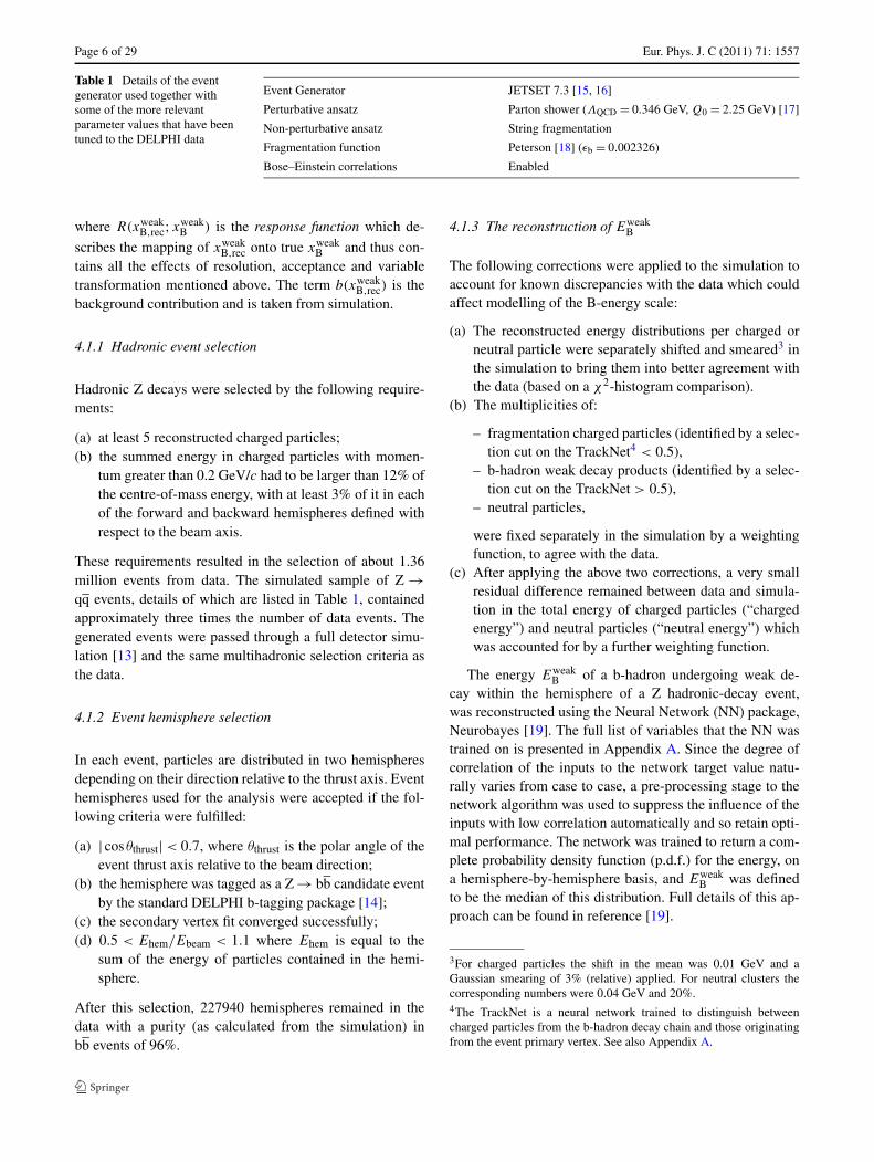
The precision of the resulting estimator, based on a statis-tically independent simulated event sample to that used fortraining and after all analysis selection cuts have been ap-plied, is shown in Fig. 1. The full width at half maximumis 14.0%.

4.1.4 The unfolding method

The solution of (5) for f (xweakB ) is a non-trivial problem

since the solution can be highly oscillatory. A practical solu-tion to this is provided by the RUN (Regularised UNfolding)program [20] which applies regularisation techniques to im-pose the condition that the solution must be smooth. In prac-tice, the algorithm defines a function W(xweak

B ) used to pro-vide a weight to the simulated distribution gsim(xweak

B,rec) such

that it reproduces the data distribution g(xweakB,rec) as well as

possible, i.e. W(xweakB ) is determined by a fit to the data.

The result of the unfolding, up to a normalisation factor, isthen given by

f(xweak

B

) = W(xweak

B

) · fsim(xweak

B

)(6)

where fsim(xweakB ) is the fragmentation function used to gen-

erate the simulated events. By summing over bins in xweakB ,

unfolded binned points are determined together with a com-plete covariance matrix.

It is important to note that internally to RUN, the weightfactors are defined as a sum over orthogonal polynomialstaken to be basis splines P(xweak

B ),

W(xweak

B

) =m∑

j=1

aj · Pj

(xweak

B

)(7)

where aj are suitable expansion coefficients. Consequently,the difficult task of solving (5) reduces to deciding at whichpoint to cutoff the sum in (7). This point, j = m, is referredto in what follows as the number of degrees of freedom of theunfolding procedure. Full details of the unfolding methodcan be found in reference [21].

Fig. 1 Distribution of the precision of the NN estimator for xweakB ,

defined as xweakB = (xweak

B,rec − xweakB,gen)/x

weakB,gen

4.1.5 Unfolding results

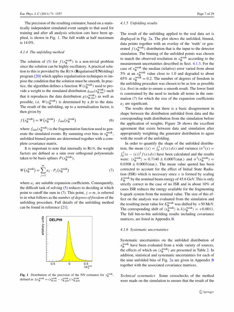
The result of the unfolding applied to the real data set isdisplayed in Fig. 2a. The plot shows the unfolded, binned,data points together with an overlay of the ‘truth’ or gen-erated f (xweak

B ) distribution that is the input to the detectorsimulation. The binning of the unfolded points was chosento match the observed resolution in xweak

B according to themeasurement uncertainties described in Sect. 4.1.3. For thecase of xweak

B the median (relative) error varied from about5% at an xweak

B value close to 1.0 and degraded to about65% at xweak

B = 0.2. The number of degrees of freedom inthe unfolding procedure was chosen to be as low as possible(i.e. five) in order to ensure a smooth result. The lower limitis constrained by the need to include all terms in the sum-mation (7) for which the size of the expansion coefficientsaj are significant.

The results show that there is a basic disagreement inshape between the distribution unfolded from data and thecorresponding truth distribution from the simulation beforethe application of weights. Figure 2b shows the excellentagreement that exists between data and simulation afterappropriately weighting the generator distribution to agreewith the result of the unfolding.

In order to quantify the shape of the unfolded distribu-tion, the mean (〈x〉 = ∫ 1

0 xf (x)dx) and variance (σ 2(x) =∫ 10 (x − 〈x〉)2f (x)dx) have been calculated and the results

were: 〈xweakB 〉 = 0.7140 ± 0.0007(stat.) and σ 2(xweak

B ) =0.0308 ± 0.0003(stat.). The mean value quoted has beencorrected to account for the effect of Initial State Radia-tion (ISR) which is necessary since x is formed by scalingEweak

B by the nominal beam energy of 45.6 GeV. This is onlystrictly correct in the case of no ISR and in about 10% ofcases ISR reduces the energy available for the fragmentingb-quark system from the nominal value. The size of this ef-fect on the analysis was evaluated from the simulation andthe resulting mean value for Eweak

B was shifted by +50 MeV.The corresponding shift of 〈xweak

B 〉 is δ〈xweakB 〉 = +0.0011.

The full bin-to-bin unfolding results including covariancematrices, are listed in Appendix B.

4.1.6 Systematic uncertainties

Systematic uncertainties on the unfolded distribution ofxweak

B have been evaluated from a wide variety of sources,the effects of which on 〈xweak

B 〉 are presented in Table 2. Inaddition, statistical and systematic uncertainties for each ofthe nine unfolded bins of Fig. 2a are given in Appendix Btogether with the associated covariance matrices.

Technical systematics Some crosschecks of the methodwere made on the simulation to ensure that the result of the

Page 8 of 29 Eur. Phys. J. C (2011) 71: 1557

Fig. 2 (a) The result ofunfolding xweak

B from real data(points), and the generator-levelfsim(xweak

B ) distribution, beforeapplying weights (curve).(b) Distribution of xweak

B in thedata, g(xweak

B,rec), compared toboth the default simulationgsim(xweak

B,rec) and the simulationweighted for the results of thefragmentation functionunfolding result shown in (a)

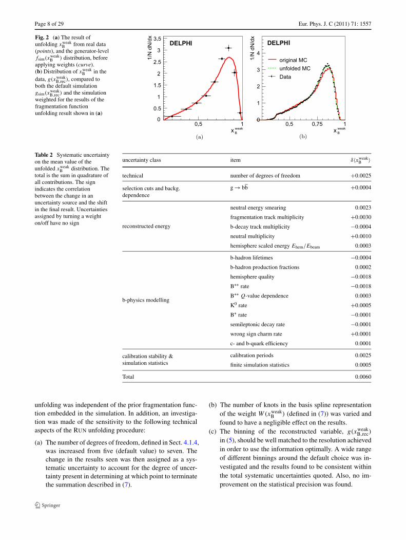
Table 2 Systematic uncertaintyon the mean value of theunfolded xweak

B distribution. Thetotal is the sum in quadrature ofall contributions. The signindicates the correlationbetween the change in anuncertainty source and the shiftin the final result. Uncertaintiesassigned by turning a weighton/off have no sign

uncertainty class item δ〈xweakB 〉

technical number of degrees of freedom +0.0025

selection cuts and backg.dependence

g → bb +0.0004

reconstructed energy

neutral energy smearing 0.0023

fragmentation track multiplicity +0.0030

b-decay track multiplicity −0.0004

neutral multiplicity +0.0010

hemisphere scaled energy Ehem/Ebeam 0.0003

b-physics modelling

b-hadron lifetimes −0.0004

b-hadron production fractions 0.0002

hemisphere quality −0.0018

B∗∗ rate −0.0018

B∗∗ Q-value dependence 0.0003

K0 rate +0.0005

B∗ rate −0.0001

semileptonic decay rate −0.0001

wrong sign charm rate +0.0001

c- and b-quark efficiency 0.0001

calibration stability &simulation statistics

calibration periods 0.0025

finite simulation statistics 0.0005

Total 0.0060

unfolding was independent of the prior fragmentation func-tion embedded in the simulation. In addition, an investiga-tion was made of the sensitivity to the following technicalaspects of the RUN unfolding procedure:

(a) The number of degrees of freedom, defined in Sect. 4.1.4,was increased from five (default value) to seven. Thechange in the results seen was then assigned as a sys-tematic uncertainty to account for the degree of uncer-tainty present in determining at which point to terminatethe summation described in (7).

(b) The number of knots in the basis spline representationof the weight W(xweak

B ) (defined in (7)) was varied andfound to have a negligible effect on the results.

(c) The binning of the reconstructed variable, g(xweakB,rec)

in (5), should be well matched to the resolution achievedin order to use the information optimally. A wide rangeof different binnings around the default choice was in-vestigated and the results found to be consistent withinthe total systematic uncertainties quoted. Also, no im-provement on the statistical precision was found.

Eur. Phys. J. C (2011) 71: 1557 Page 9 of 29

Selection cuts and background dependence The hemi-sphere selection described in Sect. 4.1.2, includes selec-tion cuts for bb event enhancement and on the reconstructedscaled hemisphere energy Ehem/Ebeam, both of which couldpotentially have an effect on the analysis if not accuratelymodelled in the simulation. The DELPHI b-tagging is basedon impact parameter measurements which degrade at lowmomenta due to the increased effects of multiple scattering.This effect correlates the b-tagging information to the B-energy. Any variation in the unfolding result was checkedwhen scanned over a wide range of b-tagging selection cutsi.e. different bb purities. The results were found to be sta-ble around the working point of bb purity ≈96%. In addi-tion, the effect of scanning around the nominal selection cutvalue of Ehem/Ebeam = 0.5 was investigated and the resultsfound to be stable. No explicit systematic was assigned dueto these two analysis selection cuts.

Uncertainties in the size and composition of the back-ground, i.e. b(xweak

B,rec) in (5), were also evaluated. Approx-

imately 75% of the background was from non-bb events,primarily cc events, which was accounted for as one of theb-physics modelling weights described later. The remain-der was composed of cases where both b-quarks were foundin the same hemisphere which occasionally happens e.g. inthree-jet events or when a gluon splits into two b-quarksleaving a topology with four b-quarks in the initial state. Inthese cases, which occur in about 2% of all hemispheres, theconnection between the generated b-hadron energy and thereconstructed quantity becomes confused and hence wereassigned to the background. It is assumed that the overall jetrate is well modelled in the simulation but the gluon split-ting rate to bb is varied, from the default value of 0.5% by±50% [22], and the change seen in the unfolding result isrecorded as a systematic uncertainty.

Reconstructed energy The relationship between the recon-structed variable distribution in the simulation, gsim(xweak

B,rec),

and the underlying physics p.d.f., fsim(xweakB ), is

gsim(xweak

B,rec

) =∫

R(xweak

B,rec;xweakB

)fsim

(xweak

B

)dxweak

B , (8)

where R(xweakB,rec;xweak

B ) is the response function definedin (5). The unfolding is, by construction, insensitive to de-tails of the prior fragmentation function fsim(xweak

B ) but onlyunder the assumption that the response function, as derivedfrom the simulation, is correct. It is therefore crucial thatR(xweak

B,rec;xweakB ) be as close to the situation in the data as

possible.Separate uncertainty contributions were assigned for

each of the three corrections, described in Sect. 4.1.3, thataffect directly modelling of the B-energy scale. Half ofthe full change in the result was taken as an uncertainty

when: (a) the shifting/smearing procedure was turned off,(b) the spread of the multiplicity weights of about 1.0 waschanged by ±50% and (c) the hemisphere energy weightwas switched off.

Since the multiplicity tuning was dependent on a specificselection cut on the TrackNet variable around the 0.5 point,it was checked that the results were not a strong functionof this choice. The multiplicity weights were recalculatedbased on considering three regions in the TrackNet variablei.e. TrackNet < 0.2, 0.2 < TrackNet < 0.8 and TrackNet >

0.8 and the analysis repeated. The results were found to beconsistent to well within the quoted systematic uncertaintiesand no additional uncertainty was assigned.

A further crosscheck was made by using a differentchoice for Eweak

B other than the Bayesian neural networkvariable described in Sect. 4.1.3. For this test, Eweak

B was es-timated by applying a rapidity algorithm (described in Ap-pendix A) and corrected for missing neutral energy basedon a parameterisation from the simulation. A detailed de-scription of this correction is given elsewhere [23]. Repeat-ing the analysis, the change seen in the result for xweak

B was−0.0011, well contained within the assigned total system-atic uncertainty.

b-physics modelling The remaining systematic contri-butions concern quantities for which the simulation wasweighted in order to account for known discrepancies withthe data. Weights were constructed to change the lifetimesand production fractions of the b-hadron species to more re-cent world average values [6]:

τ(B+) = 1.638 ± 0.011 ps,

f (B+) = (39.9 ± 1.1)%,

τ(B0d) = 1.530 ± 0.009 ps,

f (B0d) = (39.9 ± 1.1)%,

τ(B0s ) = 1.470 ± 0.027 ps,

f (B0s ) = (11.0 ± 1.2)%,

τ(b-baryon) = 1.383 ± 0.049 ps,

f (b-baryon) = (9.2 ± 1.9)%.

Systematic uncertainties from these sources were based onvarying them within the quoted one standard deviation un-certainties for the case of the lifetimes and by switching theweights on/off for the case of the production fractions. The‘hemisphere quality’ was a quantity flagging the presenceof potentially badly reconstructed tracks in the hemisphere.Improved agreement with the data was achieved in many re-constructed quantities by weighting the hemisphere qualitydistribution in the simulation to agree with that seen in data.The change induced by varying the spread of the weightaround 1.0 by ±50% from the nominal value was assignedas a systematic uncertainty.

Page 10 of 29 Eur. Phys. J. C (2011) 71: 1557

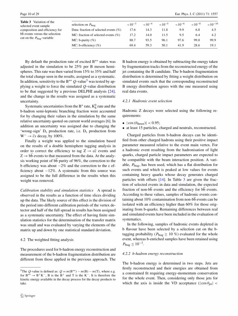
Table 3 Variation of theselected event samplecomposition and efficiency forbb events versus the selectioncut on the Pbtag-variable

selection on Pbtag <10−3 <10−4 <10−5 <10−6 <10−8 <10−10

Data: fraction of selected events (%) 17.6 14.3 11.8 9.9 6.8 4.5

MC: fraction of selected events (%) 17.2 14.0 11.5 9.5 6.4 4.2

MC: b-purity (%) 88.7 93.5 96.1 97.6 99.0 99.9

MC: b-efficiency (%) 69.4 59.3 50.1 41.9 28.6 19.1

By default the production rate of excited B∗∗ states wasadjusted in the simulation to be 25% per B meson hemi-spheres. This rate was then varied from 15% to 35% and halfthe total change seen in the results, assigned as a systematic.In addition, sensitivity to the B∗∗ Q-value5 was tested by ap-plying a weight to force the simulated Q-value distributionto be that suggested by a previous DELPHI analysis [24],and the change in the results was assigned as a systematicuncertainty.

Systematic uncertainties from the B∗ rate, K0S rate and the

b-hadron semi-leptonic branching fraction were accountedfor by changing their values in the simulation by the samerelative uncertainty quoted on current world averages [6]. Inaddition an uncertainty was assigned due to changing the‘wrong-sign’ Ds production rate, i.e. Ds production fromW− → cs decay, by 100%.

Finally a weight was applied to the simulation basedon the results of a double hemisphere tagging analysis inorder to correct the efficiency to tag Z → cc events andZ → bb events to that measured from the data. At the analy-sis working point of bb purity of 96%, the correction to theb efficiency was about −2% and the correction to the c ef-ficiency about −12%. A systematic from this source wasassigned to be the full difference in the results when thisweight was removed.

Calibration stability and simulation statistics A spread isobserved in the results as a function of time slices dividingup the data. The likely source of this effect is the division ofthe period into different calibration periods of the vertex de-tector and half of the full spread in results has been assignedas a systematic uncertainty. The effect of having finite sim-ulation statistics for the determination of the transfer matrixwas small and was evaluated by varying the elements of thematrix up and down by one statistical standard deviation.

4.2 The weighted fitting analysis

The procedures used for b-hadron energy reconstruction andmeasurement of the b-hadron fragmentation distribution aredifferent from those applied in the previous approach. The

5The Q-value is defined as: Q = m(B∗∗) − m(B) − m(T), where e.g.for B∗∗ → B+K−, B is the B+ and T is the K−. It is therefore thekinetic energy available in the decay process for the decay products totake.

B hadron energy is obtained by subtracting the energy takenby fragmentation tracks from the reconstructed energy of thejet containing the B candidate. The b-hadron fragmentationdistribution is determined by fitting a weight distribution onsimulated events such that the corresponding reconstructedB energy distribution agrees with the one measured usingreal data events.

4.2.1 Hadronic event selection

Hadronic Z decays were selected using the following re-quirements:

• | cos (θthrust)| < 0.95;• at least 15 particles, charged and neutrals, reconstructed.

Charged particles from b-hadron decays can be identi-fied from other charged hadrons using their positive impactparameter measured relative to the event main vertex. Fora hadronic event resulting from the hadronisation of lightquarks, charged particle impact parameters are expected tobe compatible with the beam interaction position. A vari-able, Pbtag, has been used, which has a flat distribution forsuch events and which is peaked at low values for eventscontaining heavy quarks whose decay generates chargedparticles with offsets [14]. In Table 3 are given the frac-tion of selected events in data and simulation, the expectedfraction of non-bb events and the efficiency for bb events.According to these values, samples of hadronic events con-taining about 10% contamination from non-bb events can beisolated with an efficiency higher than 60% for those orig-inating from b-quarks. Remaining differences between realand simulated events have been included in the evaluation ofsystematics.

In the following, samples of hadronic events depleted inb flavour have been selected by a selection cut on the b-tagging probability (Pbtag ≥ 10 %) evaluated for the wholeevent, whereas b-enriched samples have been retained usingPbtag ≤ 10−3.

4.2.2 b-hadron energy reconstruction

The b-hadron energy is determined in two steps. Jets arefirstly reconstructed and their energies are obtained froma constrained fit requiring energy-momentum conservationfor the whole event. Then, considering only those jets forwhich the axis is inside the VD acceptance (| cos θjet| <

Eur. Phys. J. C (2011) 71: 1557 Page 11 of 29

0.75), particles are classified as B decay products or frag-mentation particles. For charged particles, their offsets rel-ative to the event main vertex, and their rapidity measuredrelative to the jet axis are used in this classification, whereasfor neutrals only the rapidity is used.

Differences between real and simulated events can orig-inate from a behaviour of the detector that differs from itsexpected performances or from different particle productioncharacteristics in the events. As the reconstruction accuracyfor charged particles depends on the type of sub-detectorsused and as differences remain between the fractions of sub-detectors involved in the data and in the simulation, correc-tions have been applied. The procedure, equivalent to theremoval of a sub-detector, consists in rescaling the values ofmeasurement uncertainties and in smearing the correspond-ing track parameter values. These corrections, which applyto about 4% of all charged particles, depend on the typeof the removed sub-detector and were determined using thesimulation, by comparing uncertainty matrix elements fortracks with and without the corresponding sub-detector in-volved. In addition, as the mass distribution of reconstructedweakly decaying particles (such as those corresponding tothe D0 or D+ mesons) has a width which is larger in realdata by about 20%, a smearing corresponding to the samefraction of their measurement uncertainty has been appliedto simulated tracks.

After these corrections individual particle momentumdistributions have been compared in real and simulatedevents. These distributions considered separately for b-depleted and b-enriched samples have been normalised us-ing the respective number of selected hadronic events ineach category. To match corresponding data/simulation dis-tributions a momentum dependent correction is then applied,which consists in removing tracks alternatively in data orin the simulation depending if the measured ratio is largeror lower than unity. This correction has been determinedseparately for b-depleted and b-enriched samples and also,independently, for charged and neutral particles.

To avoid a possible bias induced by a correlation betweenthe assumed shape of the fragmentation function and the ap-plied correction, the latter has been evaluated iteratively us-ing as input in its determination the fragmentation distrib-ution measured at the previous step. In practice one itera-tion was used, as the observed absolute variation betweenthe second and first step on the resulting 〈xweak

B 〉 value wasof the order of 10−3.

In a given event, jets are reconstructed using the LundLUCLUS algorithm [25] with the djoin parameter(PARU(44)) value set to 5.0 GeV/c. A first evaluation of thejet energies is obtained using the jets directions, energies,masses and imposing total energy-momentum conservationfor the whole event. If the missing energy in a jet is largerthan 1 GeV, a 4-vector is added to the jet. Its direction istaken to be the same as the jet direction and the missing mo-mentum is evaluated assuming that the missing particle massis zero. Analysing simulated events, the relative uncertaintyon the missing energy is measured to be 20%, and uncertain-ties on angles of the missing particle are 50 mrad. Energymomentum conservation is then applied again to the wholeevent, and particle parameters (for charged, neutral and pos-sibly missing) are fitted. After this procedure, 4-vectors ofcharged and neutral particles have been fitted, and possiblynew 4-vectors corresponding to missing energy in each jethave been obtained. Jets are reevaluated (pjet) using this setof tracks and applying the same LUCLUS algorithm. Frac-tions of the fitted charged, neutral and missing energy arecompared in Table 4. Relative differences are at the levelof a few 10−3. A comparison between data and the simula-tion has been also made for the averages and variances ofcharged and neutral particle multiplicities. The results aregiven in Table 5.

Each jet pointing through the detector barrel region de-fined by | cos θjet| < 0.75 is considered in turn, and chargedparticles belonging to the jet are used to reconstruct a Bdecay vertex candidate. It is then required that these trackshave at least two VD hits associated in Rφ and a minimum

Table 4 Fitted fractions ofcharged energy (Ech.), neutralenergy (Eneu.) and their sumreconstructed in bb-depletedand bb-enriched event samplesin data and simulation. Themissing energy (Emiss.) fittedfraction is also given

bb-depleted events

Sample Ech. + Eneu. Ech. Eneu. Emiss.

Data 0.8644 0.5759 0.2879 0.1363

MC 0.8676 0.5778 0.2893 0.1323

(Data-MC)/MC −0.0037 −0.0033 −0.0048 +0.030

bb-enriched events

Sample Ech. + Eneu. Ech. Eneu. Emiss.

Data 0.8423 0.5891 0.2528 0.1589

MC 0.8423 0.5885 0.2535 0.1579

(Data-MC)/MC 0.0000 +0.0010 −0.0027 +0.0063

Page 12 of 29 Eur. Phys. J. C (2011) 71: 1557

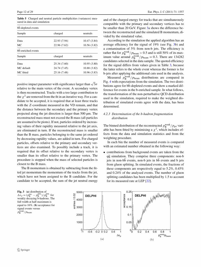
Table 5 Charged and neutral particle multiplicities (variances) mea-sured in data and simulation

bb-depleted events

Sample charged neutrals

Data 22.93 (7.94) 10.47 (3.84)

MC 22.96 (7.62) 10.56 (3.82)

bb-enriched events

Sample charged neutrals

Data 25.34 (7.60) 10.95 (3.80)

MC default 24.74 (7.45) 10.88 (3.82)

MC fitted 25.16 (7.48) 10.96 (3.83)

positive impact parameter with significance larger than√

3σ

relative to the main vertex of the event. A secondary vertexis then reconstructed. Tracks with a too large contribution tothe χ2 are removed from the fit in an iterative way. For a can-didate to be accepted, it is required that at least three trackswith the Z-coordinate measured in the VD remain, and thatthe distance between the secondary and the primary vertexprojected along the jet direction is larger than 500 µm. Thereconstructed mass must not exceed the B mass (all particlesare assumed to be pions). If not, particles ordered by increas-ing values of their rapidity measured relative to the jet axis,are eliminated in turn. If the reconstructed mass is smallerthan the B mass, particles belonging to the same jet orderedby decreasing rapidity values, are added in turn. For chargedparticles, offsets relative to the primary and secondary ver-tices are also examined. To possibly include a track, it isrequired that its offset relative to the secondary vertex issmaller than its offset relative to the primary vertex. Theprocedure is stopped when the mass of selected particles isclosest to the B mass.

The B momentum is obtained by subtracting from the fit-ted jet momentum the momentum of the tracks from the jet,which have not been assigned to the B candidate. For thecandidate to be accepted, the sum of the jet neutral energy

and of the charged energy for tracks that are simultaneouslycompatible with the primary and secondary vertices has tobe smaller than 20 GeV. Figure 3a shows the difference be-tween the reconstructed and the simulated B momentum, di-vided by the simulated value.

According to the simulation the applied algorithm has anaverage efficiency for the signal of 19% (see Fig. 3b) anda contamination of 5% from non-b jets. The efficiency israther flat for pweak

B /pbeam > 0.5 and is still 50% of its max-imum value around pweak

B /pbeam = 0.3. There are 134282candidates selected in the data sample. The quoted efficiencyfor the signal differs from values given in Table 3, becausethe latter refers to the whole event whereas the former is forb-jets after applying the additional cuts used in the analysis.

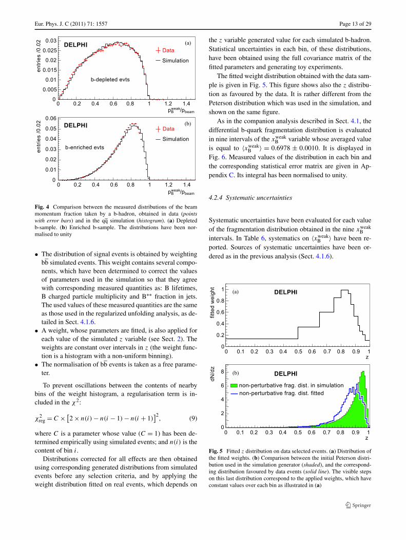
Measured pweakB /pbeam distributions are compared in

Fig. 4 with expectations from the simulation. The two distri-butions agree for bb-depleted events and show a marked dif-ference for events in the b-enriched sample. In what follows,the transformation of the non-perturbative QCD distributionused in the simulation, required to make the weighted dis-tribution of simulated events agree with the data, has beendetermined.

4.2.3 Determination of the b-hadron fragmentationdistribution

The binned distribution of the reconstructed pweakB /pjet vari-

able has been fitted by minimising a χ2, which includes ef-fects from the data and simulation statistics and from theweighting procedure.

In each bin the number of measured events is comparedwith an estimated number obtained in the following way:

• contributions from background events are taken from theqq simulation. They comprise three components: non-bjets in non-bb events, non-b jets in bb events and b jetsfrom gluon splitting. In simulated events, the fractions ofthese components are respectively equal to 5.2%, 0.45%and 0.24% of the analysed events. The number of gluonsplitting candidates has been multiplied by 1.5 to accountfor its measured rate at LEP [22].

Fig. 3 (a) distribution ofxp = (prec.

B − pgen.B )/p

gen.B for

weakly decaying b-hadrons. Thefull width at half maximum isequal to 16%. (b) acceptance forsignal events versuspweak

B /pbeam

Eur. Phys. J. C (2011) 71: 1557 Page 13 of 29

Fig. 4 Comparison between the measured distributions of the beammomentum fraction taken by a b-hadron, obtained in data (pointswith error bars) and in the qq simulation (histogram). (a) Depletedb-sample. (b) Enriched b-sample. The distributions have been nor-malised to unity

• The distribution of signal events is obtained by weightingbb simulated events. This weight contains several compo-nents, which have been determined to correct the valuesof parameters used in the simulation so that they agreewith corresponding measured quantities as: B lifetimes,B charged particle multiplicity and B∗∗ fraction in jets.The used values of these measured quantities are the sameas those used in the regularized unfolding analysis, as de-tailed in Sect. 4.1.6.

• A weight, whose parameters are fitted, is also applied foreach value of the simulated z variable (see Sect. 2). Theweights are constant over intervals in z (the weight func-tion is a histogram with a non-uniform binning).

• The normalisation of bb events is taken as a free parame-ter.

To prevent oscillations between the contents of nearbybins of the weight histogram, a regularisation term is in-cluded in the χ2:

χ2reg = C × [

2 × n(i) − n(i − 1) − n(i + 1)]2

, (9)

where C is a parameter whose value (C = 1) has been de-termined empirically using simulated events; and n(i) is thecontent of bin i.

Distributions corrected for all effects are then obtainedusing corresponding generated distributions from simulatedevents before any selection criteria, and by applying theweight distribution fitted on real events, which depends on

the z variable generated value for each simulated b-hadron.Statistical uncertainties in each bin, of these distributions,have been obtained using the full covariance matrix of thefitted parameters and generating toy experiments.

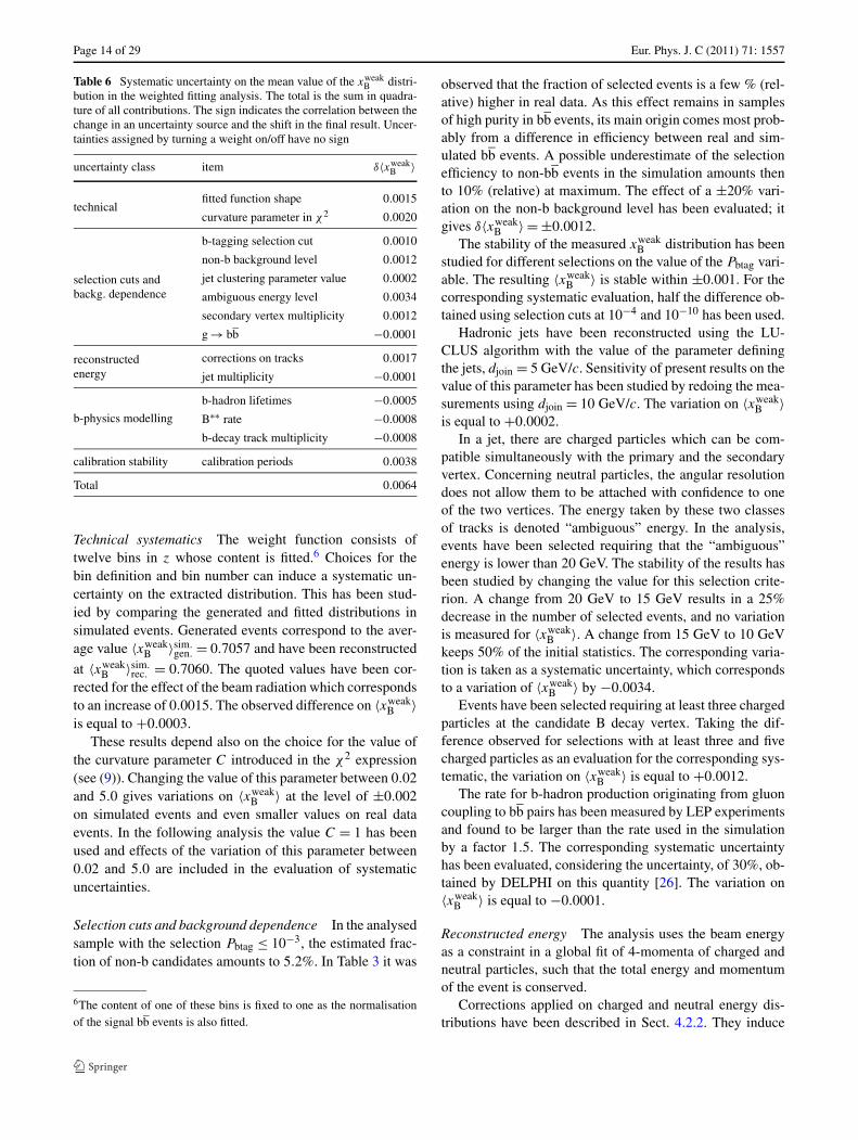
The fitted weight distribution obtained with the data sam-ple is given in Fig. 5. This figure shows also the z distribu-tion as favoured by the data. It is rather different from thePeterson distribution which was used in the simulation, andshown on the same figure.

As in the companion analysis described in Sect. 4.1, thedifferential b-quark fragmentation distribution is evaluatedin nine intervals of the xweak

B variable whose averaged valueis equal to 〈xweak

B 〉 = 0.6978 ± 0.0010. It is displayed inFig. 6. Measured values of the distribution in each bin andthe corresponding statistical error matrix are given in Ap-pendix C. Its integral has been normalised to unity.

4.2.4 Systematic uncertainties

Systematic uncertainties have been evaluated for each valueof the fragmentation distribution obtained in the nine xweak

Bintervals. In Table 6, systematics on 〈xweak

B 〉 have been re-ported. Sources of systematic uncertainties have been or-dered as in the previous analysis (Sect. 4.1.6).

Fig. 5 Fitted z distribution on data selected events. (a) Distribution ofthe fitted weights. (b) Comparison between the initial Peterson distri-bution used in the simulation generator (shaded), and the correspond-ing distribution favoured by data events (solid line). The visible stepson this last distribution correspond to the applied weights, which haveconstant values over each bin as illustrated in (a)

Page 14 of 29 Eur. Phys. J. C (2011) 71: 1557

Table 6 Systematic uncertainty on the mean value of the xweakB distri-

bution in the weighted fitting analysis. The total is the sum in quadra-ture of all contributions. The sign indicates the correlation between thechange in an uncertainty source and the shift in the final result. Uncer-tainties assigned by turning a weight on/off have no sign

uncertainty class item δ〈xweakB 〉

technicalfitted function shape 0.0015

curvature parameter in χ2 0.0020

selection cuts andbackg. dependence

b-tagging selection cut 0.0010

non-b background level 0.0012

jet clustering parameter value 0.0002

ambiguous energy level 0.0034

secondary vertex multiplicity 0.0012

g → bb −0.0001

reconstructedenergy

corrections on tracks 0.0017

jet multiplicity −0.0001

b-physics modelling

b-hadron lifetimes −0.0005

B∗∗ rate −0.0008

b-decay track multiplicity −0.0008

calibration stability calibration periods 0.0038

Total 0.0064

Technical systematics The weight function consists oftwelve bins in z whose content is fitted.6 Choices for thebin definition and bin number can induce a systematic un-certainty on the extracted distribution. This has been stud-ied by comparing the generated and fitted distributions insimulated events. Generated events correspond to the aver-age value 〈xweak

B 〉sim.gen. = 0.7057 and have been reconstructed

at 〈xweakB 〉sim.

rec. = 0.7060. The quoted values have been cor-rected for the effect of the beam radiation which correspondsto an increase of 0.0015. The observed difference on 〈xweak

B 〉is equal to +0.0003.

These results depend also on the choice for the value ofthe curvature parameter C introduced in the χ2 expression(see (9)). Changing the value of this parameter between 0.02and 5.0 gives variations on 〈xweak

B 〉 at the level of ±0.002on simulated events and even smaller values on real dataevents. In the following analysis the value C = 1 has beenused and effects of the variation of this parameter between0.02 and 5.0 are included in the evaluation of systematicuncertainties.

Selection cuts and background dependence In the analysedsample with the selection Pbtag ≤ 10−3, the estimated frac-tion of non-b candidates amounts to 5.2%. In Table 3 it was

6The content of one of these bins is fixed to one as the normalisationof the signal bb events is also fitted.

observed that the fraction of selected events is a few % (rel-ative) higher in real data. As this effect remains in samplesof high purity in bb events, its main origin comes most prob-ably from a difference in efficiency between real and sim-ulated bb events. A possible underestimate of the selectionefficiency to non-bb events in the simulation amounts thento 10% (relative) at maximum. The effect of a ±20% vari-ation on the non-b background level has been evaluated; itgives δ〈xweak

B 〉 = ±0.0012.The stability of the measured xweak

B distribution has beenstudied for different selections on the value of the Pbtag vari-able. The resulting 〈xweak

B 〉 is stable within ±0.001. For thecorresponding systematic evaluation, half the difference ob-tained using selection cuts at 10−4 and 10−10 has been used.

Hadronic jets have been reconstructed using the LU-CLUS algorithm with the value of the parameter definingthe jets, djoin = 5 GeV/c. Sensitivity of present results on thevalue of this parameter has been studied by redoing the mea-surements using djoin = 10 GeV/c. The variation on 〈xweak

B 〉is equal to +0.0002.

In a jet, there are charged particles which can be com-patible simultaneously with the primary and the secondaryvertex. Concerning neutral particles, the angular resolutiondoes not allow them to be attached with confidence to oneof the two vertices. The energy taken by these two classesof tracks is denoted “ambiguous” energy. In the analysis,events have been selected requiring that the “ambiguous”energy is lower than 20 GeV. The stability of the results hasbeen studied by changing the value for this selection crite-rion. A change from 20 GeV to 15 GeV results in a 25%decrease in the number of selected events, and no variationis measured for 〈xweak

B 〉. A change from 15 GeV to 10 GeVkeeps 50% of the initial statistics. The corresponding varia-tion is taken as a systematic uncertainty, which correspondsto a variation of 〈xweak

B 〉 by −0.0034.Events have been selected requiring at least three charged

particles at the candidate B decay vertex. Taking the dif-ference observed for selections with at least three and fivecharged particles as an evaluation for the corresponding sys-tematic, the variation on 〈xweak

B 〉 is equal to +0.0012.The rate for b-hadron production originating from gluon

coupling to bb pairs has been measured by LEP experimentsand found to be larger than the rate used in the simulationby a factor 1.5. The corresponding systematic uncertaintyhas been evaluated, considering the uncertainty, of 30%, ob-tained by DELPHI on this quantity [26]. The variation on〈xweak

B 〉 is equal to −0.0001.

Reconstructed energy The analysis uses the beam energyas a constraint in a global fit of 4-momenta of charged andneutral particles, such that the total energy and momentumof the event is conserved.

Corrections applied on charged and neutral energy dis-tributions have been described in Sect. 4.2.2. They induce

Eur. Phys. J. C (2011) 71: 1557 Page 15 of 29

a variation on 〈xweakB 〉 of +0.0017. The corresponding sys-

tematic uncertainty has been evaluated taking the effect ofthis correction.

Measured jet multiplicities are not identical in data andin simulated events. Taking as reference the fraction of two-jet events, fractions of three- and four-jet events have to becorrected respectively by −5% and +13% in the simula-tion. Simulated events have been weighted accordingly sothat the two distributions agree. From the statistical accu-racy of this correction, the systematic uncertainty has beenevaluated to be one third of the correction. This correspondsto δ〈xweak

B 〉 = −0.0001.

b-physics modelling Variations of the values of parametersthat govern decay properties or production characteristics ofb-hadrons have been also considered.

Simulated events have been generated using the samelifetime value of τB = 1.6 ps. Events have been weightedsuch that each type of b-hadron is distributed according toits corresponding lifetime, as given in reference [6]. Taking,as systematics, the total variation induced by this correction,the variation on 〈xweak

B 〉 is equal to −0.0005.In the simulation, the B∗∗ production rate in a b-quark jet

amounts to 32%. A weight is applied on b-hadrons whichoriginate from B∗∗ decays to lower the effective B∗∗ rate to25%. The corresponding systematic has been taken as thevariation on 〈xweak

B 〉, namely −0.0008.The difference between simulated, nsim

ch (B), and mea-sured, nmeas

ch (B), average charged multiplicities in b-hadrondecays amounts to 0.06:

nmeasch (B) = 4.97 ± 0.03 ± 0.06, nsim

ch (B) = 4.91. (10)

This difference has been corrected by weighting events us-ing a weight that has a linear variation with the actual b-hadron charged multiplicity in a given event. The simulatedmultiplicity distribution has been fitted with a Gaussian ofstandard deviation (σnch) equal to 2.03 charged particles.Probability values, for a given charged multiplicity i, Pi,

have been transformed into:

P Ti = Pi

[1 + β(nsim

ch − i)]. (11)

The value of β is obtained by requiring that the new averagemultiplicity computed using P T

i is equal to nmeasch (B). Then:

β = nsimch − nmeas

ch

σ 2nch

. (12)

The corresponding systematic uncertainty has been evalu-ated by considering an uncertainty of ±0.1 charged particleson nmeas

ch . The variation on 〈xweakB 〉 is equal to ∓0.0008.

Calibration stability and simulation statistics The stabil-ity of the energy calibration has been studied dividing theanalysed data samples in five time ordered subsamples ofsimilar statistics. The statistical accuracy of each 〈xweak

B 〉measurement is of about 0.002. The systematic uncertaintyattached to the energy reconstruction has been evaluated bytaking half the difference between the two extremes of thefive measurements of 〈xweak

B 〉: ±0.0038.Uncertainties corresponding to the finite statistics of sim-

ulated events have been included in the statistical uncer-tainty of the measurements.

4.3 Combination of the xweakB distributions

The results of the two xweakB measurements obtained in

Sects. 4.1 and 4.2 have been averaged. In this combinationa complete correlation has been assumed between statisti-cal uncertainties, due to the common data used by the twoanalyses. The following sources of systematic uncertaintieshave been considered also as fully correlated:

• neutral energy smearing in the regularised unfoldinganalysis with ambiguous energy level in the weighted fit-ting analysis;

• g → bb branching fraction;• B∗∗ production rate;• b-hadron lifetimes;• b-decay track multiplicity;• b-hadron production fractions;• wrong sign charm rate.

Other systematic uncertainties, some of them large, havebeen taken as uncorrelated as the two analyses are us-ing different techniques. No significant correlation was ob-served between the two measurements when consideringevent samples recorded during the same time periods.

The combined xweakB distribution has been obtained by a

fit using the full error matrix of the two analyses. This matrixhas two insignificant eigenvalues which have been removed.The fit has therefore 7 degrees of freedom and the χ2 valueis 11.96 (probability of 10.2%).

The combined value of the f (xweakB ) distribution in each

bin is given in Table 7 and in Fig. 6. The corresponding sta-tistical and total error matrices are given in Appendix D. Inthe following, all the quoted uncertainties on the f (xweak

B )

distribution bins are scaled by 1.31. This corresponds toχ2/NDF = 1. By rescaling the uncertainties it is ensuredthat possible poor fit probabilities of models with the com-bined measurement do not originate from an underestimateof quoted measurement uncertainties. The average value ofthis distribution is equal to:⟨xweak

B

⟩ = 0.699 ± 0.011. (13)

This value is largely influenced by correlations between thexweak

B distributions from the two analyses.

Page 16 of 29 Eur. Phys. J. C (2011) 71: 1557

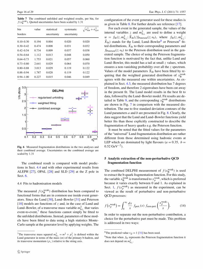
Table 7 The combined unfolded and weighted results, per bin, forf (xweak

B ). Quoted uncertainties have been scaled by 1.31

bin value statistical systematic√

σ 2stat + σ 2

syst

borders uncertainty uncertainty

0.10–0.30 0.194 0.004 0.020 0.020

0.30–0.42 0.474 0.008 0.031 0.032

0.42–0.54 0.734 0.009 0.037 0.038

0.54–0.64 1.112 0.013 0.048 0.050

0.64–0.73 1.753 0.021 0.057 0.060

0.73–0.80 2.641 0.029 0.064 0.070

0.80–0.88 3.013 0.029 0.119 0.122

0.88–0.94 1.787 0.028 0.119 0.122

0.94–1.00 0.227 0.015 0.046 0.049

Fig. 6 Measured fragmentation distributions in the two analyses andtheir combined average. Uncertainties on the combined average arescaled by 1.31

The combined result is compared with model predic-tions in Sect. 4.4 and with other experimental results fromALEPH [27], OPAL [28] and SLD [29] at the Z pole inSect. 6.

4.4 Fits to hadronisation models

The measured f (xweakB ) distribution has been compared to

functional forms that are in common use inside event gener-ators. Since the Lund [30], Lund–Bowler [31] and Peterson[18] models are functions of z and, in the case of Lund andLund–Bowler, of a transverse mass variable m2

b⊥ that variesevent-to-event,7 these functions cannot simply be fitted tothe unfolded distributions. Instead, parameters of these mod-els have been fitted to data using a high statistics Monte-Carlo sample at the generator level by applying weights. The

7The transverse mass squared m2b⊥ = m2 + p2⊥ is defined within the

Lund generator in terms of the mass (m) of the primary b-hadron, andits transverse momentum (p⊥) relative to the string axis.

configuration of the event generator used for these studies isas given in Table 8. For further details see reference [17].

For each event in the generated sample, the values of theinternal variables z and m2

b⊥ are used to define a weightw = ffit(z,m

2b⊥; �Xfit)/fPeterson(z; εb), where ffit(z,m

2b⊥;

�Xfit) stands for the Lund, Lund–Bowler8 or Peterson9 fit-ted distributions, �Xfit to their corresponding parameters andfPeterson(z; εb) to the Peterson distribution used in the gen-erated sample. The choice of using the Peterson fragmenta-tion function is motivated by the fact that, unlike Lund andLund–Bowler, this model has a tail at small z values, whichensures a non-vanishing probability over all the z spectrum.Values of the model parameters �Xfit have been fitted by re-quiring that the weighted generated distribution of xweak

Bagrees with the measured one within uncertainties. As ex-plained in Sect. 4.3, the measured distribution has 7 degreesof freedom, and therefore 2 eigenvalues have been cut awayin the present fit. The Lund model results in the best fit todata, followed by the Lund–Bowler model. Fit results are de-tailed in Table 9, and the corresponding xweak

B distributionsare shown in Fig. 7 in comparison with the measured dis-tribution. The one to five standard deviation contours of theLund parameters a and b are presented in Fig. 8. Clearly, thedata suggest that the Lund and Lund–Bowler functions yieldbetter fits than those explicitly constructed to describe thefragmentation of heavy quarks e.g. the Peterson function.

It must be noted that the fitted values for the parametersof the “universal” Lund fragmentation distribution are ratherdifferent from those determined using hadronic events atLEP which are dominated by light flavours (a = 0.35, b =0.52 GeV−2).

5 Analytic extraction of the non-perturbative QCDfragmentation function

The combined DELPHI measurement of f (xweakB ) is used

to extract the b-quark fragmentation function. For this study,the variable xweak

B is transformed to xweakp , which is preferred

because it varies exactly between 0 and 1. As explained inSect. 1, f (xweak

p ) as measured in the experiment, can beviewed as the result of perturbative and non-perturbativeQCD processes:

f(xweakp

) =∫ ∞

0

dx

xfpert.(x) fnon-pert.

(xweakp

x

). (14)

In order to separate out the non-perturbative contribution, achoice for the perturbative part must be made. This problemis addressed in two ways:

8The predicted value rQ = 1 [31] has been used.9Note that when ffit represents the Peterson fragmentation function itdoes not depend on m2

b⊥.

Eur. Phys. J. C (2011) 71: 1557 Page 17 of 29

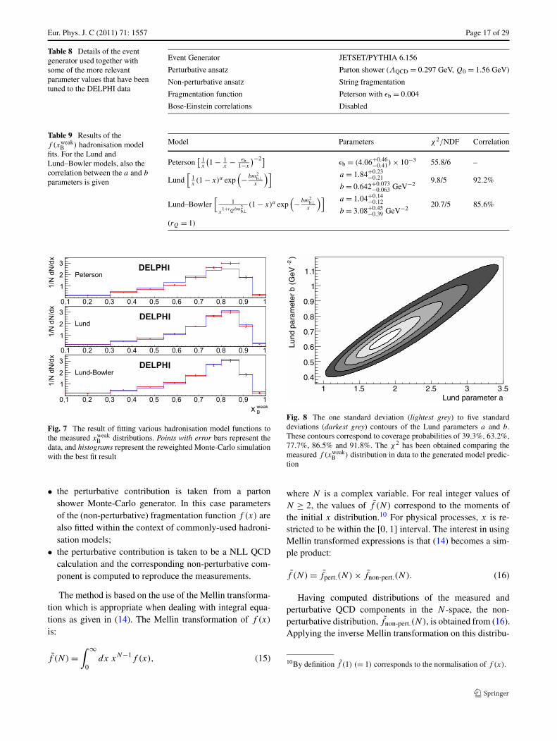
Table 8 Details of the eventgenerator used together withsome of the more relevantparameter values that have beentuned to the DELPHI data

Event Generator JETSET/PYTHIA 6.156

Perturbative ansatz Parton shower (ΛQCD = 0.297 GeV, Q0 = 1.56 GeV)

Non-perturbative ansatz String fragmentation

Fragmentation function Peterson with εb = 0.004

Bose-Einstein correlations Disabled

Table 9 Results of thef (xweak

B ) hadronisation modelfits. For the Lund andLund–Bowler models, also thecorrelation between the a and b

parameters is given

Model Parameters χ2/NDF Correlation

Peterson[ 1

x

(1 − 1

x− εb

1−x

)−2]εb = (4.06+0.46

−0.41) × 10−3 55.8/6 –

Lund[

1x(1 − x)a exp

(− bm2

b⊥x

)] a = 1.84+0.23−0.21

b = 0.642+0.073−0.063 GeV−2

9.8/5 92.2%

Lund–Bowler[

1

x1+rQbm2

b⊥(1 − x)a exp

(− bm2

b⊥x

)] a = 1.04+0.14−0.12

b = 3.08+0.45−0.39 GeV−2

20.7/5 85.6%

(rQ = 1)

Fig. 7 The result of fitting various hadronisation model functions tothe measured xweak

B distributions. Points with error bars represent thedata, and histograms represent the reweighted Monte-Carlo simulationwith the best fit result

• the perturbative contribution is taken from a partonshower Monte-Carlo generator. In this case parametersof the (non-perturbative) fragmentation function f (x) arealso fitted within the context of commonly-used hadroni-sation models;

• the perturbative contribution is taken to be a NLL QCDcalculation and the corresponding non-perturbative com-ponent is computed to reproduce the measurements.

The method is based on the use of the Mellin transforma-tion which is appropriate when dealing with integral equa-tions as given in (14). The Mellin transformation of f (x)

is:

f (N) =∫ ∞

0dx xN−1f (x), (15)

Fig. 8 The one standard deviation (lightest grey) to five standarddeviations (darkest grey) contours of the Lund parameters a and b.These contours correspond to coverage probabilities of 39.3%, 63.2%,77.7%, 86.5% and 91.8%. The χ2 has been obtained comparing themeasured f (xweak

B ) distribution in data to the generated model predic-tion

where N is a complex variable. For real integer values ofN ≥ 2, the values of f (N) correspond to the moments ofthe initial x distribution.10 For physical processes, x is re-stricted to be within the [0,1] interval. The interest in usingMellin transformed expressions is that (14) becomes a sim-ple product:

f (N) = fpert.(N) × fnon-pert.(N). (16)

Having computed distributions of the measured andperturbative QCD components in the N -space, the non-perturbative distribution, fnon-pert.(N), is obtained from (16).Applying the inverse Mellin transformation on this distribu-

10By definition f (1) (= 1) corresponds to the normalisation of f (x).

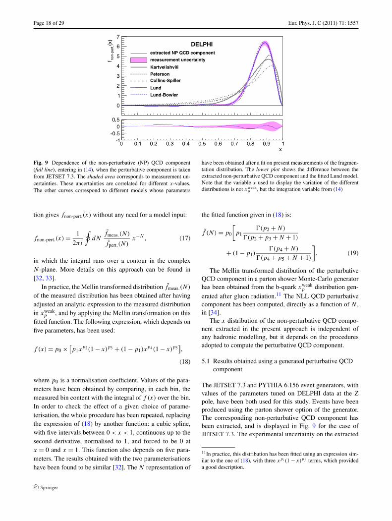
Page 18 of 29 Eur. Phys. J. C (2011) 71: 1557

Fig. 9 Dependence of the non-perturbative (NP) QCD component(full line), entering in (14), when the perturbative component is takenfrom JETSET 7.3. The shaded area corresponds to measurement un-certainties. These uncertainties are correlated for different x-values.The other curves correspond to different models whose parameters

have been obtained after a fit on present measurements of the fragmen-tation distribution. The lower plot shows the difference between theextracted non-perturbative QCD component and the fitted Lund model.Note that the variable x used to display the variation of the differentdistributions is not xweak

p , but the integration variable from (14)

tion gives fnon-pert.(x) without any need for a model input:

fnon-pert.(x) = 1

2πi

∮dN

fmeas.(N)

fpert.(N)x−N, (17)

in which the integral runs over a contour in the complexN -plane. More details on this approach can be found in[32, 33].

In practice, the Mellin transformed distribution fmeas.(N)

of the measured distribution has been obtained after havingadjusted an analytic expression to the measured distributionin xweak

p , and by applying the Mellin transformation on thisfitted function. The following expression, which depends onfive parameters, has been used:

f (x) = p0 × [p1x

p2(1 − x)p3 + (1 − p1)xp4(1 − x)p5

],

(18)

where p0 is a normalisation coefficient. Values of the para-meters have been obtained by comparing, in each bin, themeasured bin content with the integral of f (x) over the bin.In order to check the effect of a given choice of parame-terisation, the whole procedure has been repeated, replacingthe expression of (18) by another function: a cubic spline,with five intervals between 0 < x < 1, continuous up to thesecond derivative, normalised to 1, and forced to be 0 atx = 0 and x = 1. This function also depends on five para-meters. The results obtained with the two parameterisationshave been found to be similar [32]. The N representation of

the fitted function given in (18) is:

f (N) = p0

[p1

�(p2 + N)

�(p2 + p3 + N + 1)

+ (1 − p1)�(p4 + N)

�(p4 + p5 + N + 1)

]. (19)

The Mellin transformed distribution of the perturbativeQCD component in a parton shower Monte-Carlo generatorhas been obtained from the b-quark xweak

p distribution gen-

erated after gluon radiation.11 The NLL QCD perturbativecomponent has been computed, directly as a function of N ,in [34].

The x distribution of the non-perturbative QCD compo-nent extracted in the present approach is independent ofany hadronic modelling, but it depends on the proceduresadopted to compute the perturbative QCD component.

5.1 Results obtained using a generated perturbative QCDcomponent

The JETSET 7.3 and PYTHIA 6.156 event generators, withvalues of the parameters tuned on DELPHI data at the Zpole, have been both used for this study. Events have beenproduced using the parton shower option of the generator.The corresponding non-perturbative QCD component hasbeen extracted, and is displayed in Fig. 9 for the case ofJETSET 7.3. The experimental uncertainty on the extracted

11In practice, this distribution has been fitted using an expression sim-ilar to the one of (18), with three xpi (1 − x)pj terms, which provideda good description.

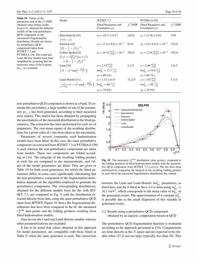
Eur. Phys. J. C (2011) 71: 1557 Page 19 of 29

Table 10 Values of theparameters and of the χ2/NDFobtained when fitting resultsfrom (14), obtained for differentmodels of the non-perturbativeQCD component, to themeasured b-fragmentationdistribution. Results are shownfor perturbative QCDcomponents taken fromJETSET 7.3 andPYTHIA 6.156. The Lund andLund–Bowler models have beensimplified by assuming that thetransverse mass of the b-quark,mb⊥, is a constant

Model JETSET 7.3 PYTHIA 6.156

Fitted Parameters andCorrelation (ρ)

χ2/NDF Fitted Parameters andCorrelation (ρ)

χ2/NDF

Kartvelishvili [35] εb = 10.17 ± 0.37 126/6 εb = 13.50 ± 0.56 57/6

xεb (1 − x)

Peterson [18] εb = (7.4 ± 0.6) × 10−3 83/6 εb = (4.4 ± 0.4) × 10−3 153/61x

(1 − 1

x− εb

1−x

)−2

Collins-Spiller[36] εb = (6.74+0.72−0.64) × 10−3 358/6 εb = (2.56+0.38

−0.32) × 10−3 322/6( 1−xx

+ εb(2−x)1−x

)(1 + x2)

× (1 − 1

x− εb

1−x

)−2

Lund [30] a = 2.35+0.25−0.22 2.3/5 a = 2.06+0.28

−0.24 3.8/51x(1 − x)a exp

(− bm2

b⊥x

)bm2

b⊥ = 17.7+1.9−1.6 bm2

b⊥ = 19.8+2.4−2.0

(ρ = 89.1%) (ρ = 89.7%)

Lund–Bowler [31] a = 1.32 ± 0.14 12.2/5 a = 1.02+0.15−0.13 5.1/5

1

x1+bm2

b⊥(1 − x)a exp

(− bm2

b⊥x

)bm2

b⊥ = 80.+12.−11. bm2

b⊥ = 95.+13.−12.

(ρ = 75.0%) (ρ = 76.5%)

non-perturbative QCD component is shown as a band. To es-timate this uncertainty, a large number of sets of the parame-ters p1,..,5 has been generated, according to their measurederror matrix. This matrix has been obtained by propagatingthe uncertainties of the measured distribution to the fitted pa-rameters. The extraction has been performed for each set ofparameters. The root mean square of the resulting distribu-tions for a given value of x has been taken as the uncertainty.

Parameters of several commonly used hadronisationmodels have been fitted. In this case, the same perturbativecomponent (as extracted from JETSET 7.3 or PYTHIA 6.156)is used whereas the non-perturbative components are takenfrom models. These two components are folded accord-ing to (14). The integrals of the resulting folding productin each bin are compared to the measurements, and val-ues of the model parameters are fitted. They are given inTable 10 for both event generators, for which the fitted pa-rameters differ, in some cases significantly (illustrating thatthe non-perturbative component of the fragmentation distri-bution depends on the algorithm employed to generate theperturbative component). The corresponding distributions,obtained for the different models from the fits with JET-SET 7.3, are compared in Fig. 9 with the distribution ex-tracted directly from data, using the same perturbative QCDinput from JETSET. Figure 10 shows the fragmentation dis-tributions that have been compared in the fit: the measuredxweakp data points and the folding products resulting from

fitted hadronisation models.Data favour the Lund and Lund–Bowler models whereas

other parameterisations are excluded.It has to be noted that values obtained in this approach

for model parameters, are compatible with those listed inTable 9, when the same generator is used. The conversion

Fig. 10 The measured xweakp distribution (data points), compared to

the folding products of fitted hadronisation models with the perturba-tive QCD component from JETSET 7.3 (curves). The fits have beenperformed by comparing the integral of the resulting folding productin each bin to the measured fragmentation distribution bin content

between the Lund and Lund–Bowler bm2b⊥ parameters, as

fitted here, and the b fitted in Sect. 4.4 is done using m2b⊥ =

30.1 GeV2, which corresponds to the mean value of m2b⊥ in

the generated events. The approximation of a constant m2b⊥

is possible due to the small dispersion of this variable ingenerated events.

5.2 Results using a perturbative QCD componentobtained by an analytic computation based on QCD

The perturbative QCD fragmentation function is evaluatedaccording to the approach presented in [34]. Computationsare done directly in the N -space and are expected to be reli-able when |N | is not too large (typically less than 20). This

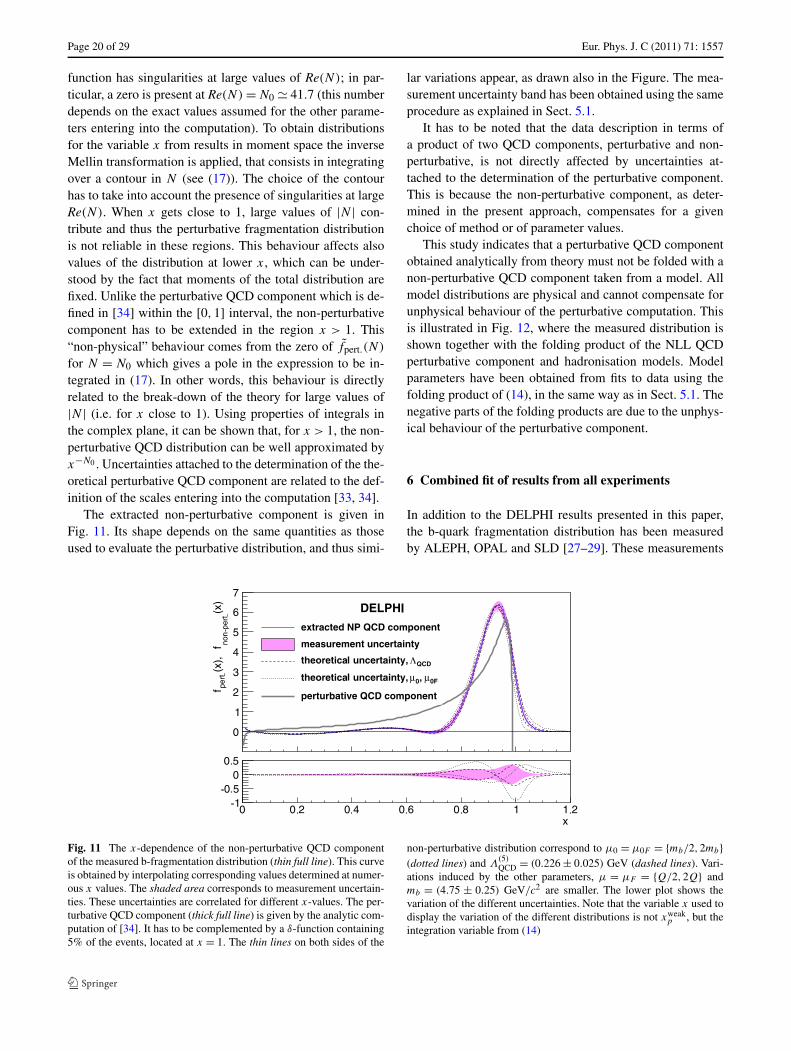
Page 20 of 29 Eur. Phys. J. C (2011) 71: 1557

function has singularities at large values of Re(N); in par-ticular, a zero is present at Re(N) = N0 � 41.7 (this numberdepends on the exact values assumed for the other parame-ters entering into the computation). To obtain distributionsfor the variable x from results in moment space the inverseMellin transformation is applied, that consists in integratingover a contour in N (see (17)). The choice of the contourhas to take into account the presence of singularities at largeRe(N). When x gets close to 1, large values of |N | con-tribute and thus the perturbative fragmentation distributionis not reliable in these regions. This behaviour affects alsovalues of the distribution at lower x, which can be under-stood by the fact that moments of the total distribution arefixed. Unlike the perturbative QCD component which is de-fined in [34] within the [0,1] interval, the non-perturbativecomponent has to be extended in the region x > 1. This“non-physical” behaviour comes from the zero of fpert.(N)

for N = N0 which gives a pole in the expression to be in-tegrated in (17). In other words, this behaviour is directlyrelated to the break-down of the theory for large values of|N | (i.e. for x close to 1). Using properties of integrals inthe complex plane, it can be shown that, for x > 1, the non-perturbative QCD distribution can be well approximated byx−N0 . Uncertainties attached to the determination of the the-oretical perturbative QCD component are related to the def-inition of the scales entering into the computation [33, 34].

The extracted non-perturbative component is given inFig. 11. Its shape depends on the same quantities as thoseused to evaluate the perturbative distribution, and thus simi-

lar variations appear, as drawn also in the Figure. The mea-surement uncertainty band has been obtained using the sameprocedure as explained in Sect. 5.1.

It has to be noted that the data description in terms ofa product of two QCD components, perturbative and non-perturbative, is not directly affected by uncertainties at-tached to the determination of the perturbative component.This is because the non-perturbative component, as deter-mined in the present approach, compensates for a givenchoice of method or of parameter values.

This study indicates that a perturbative QCD componentobtained analytically from theory must not be folded with anon-perturbative QCD component taken from a model. Allmodel distributions are physical and cannot compensate forunphysical behaviour of the perturbative computation. Thisis illustrated in Fig. 12, where the measured distribution isshown together with the folding product of the NLL QCDperturbative component and hadronisation models. Modelparameters have been obtained from fits to data using thefolding product of (14), in the same way as in Sect. 5.1. Thenegative parts of the folding products are due to the unphys-ical behaviour of the perturbative component.

6 Combined fit of results from all experiments

In addition to the DELPHI results presented in this paper,the b-quark fragmentation distribution has been measuredby ALEPH, OPAL and SLD [27–29]. These measurements

Fig. 11 The x-dependence of the non-perturbative QCD componentof the measured b-fragmentation distribution (thin full line). This curveis obtained by interpolating corresponding values determined at numer-ous x values. The shaded area corresponds to measurement uncertain-ties. These uncertainties are correlated for different x-values. The per-turbative QCD component (thick full line) is given by the analytic com-putation of [34]. It has to be complemented by a δ-function containing5% of the events, located at x = 1. The thin lines on both sides of the

non-perturbative distribution correspond to μ0 = μ0F = {mb/2,2mb}(dotted lines) and Λ

(5)QCD = (0.226 ± 0.025) GeV (dashed lines). Vari-

ations induced by the other parameters, μ = μF = {Q/2,2Q} andmb = (4.75 ± 0.25) GeV/c2 are smaller. The lower plot shows thevariation of the different uncertainties. Note that the variable x used todisplay the variation of the different distributions is not xweak

p , but theintegration variable from (14)

Eur. Phys. J. C (2011) 71: 1557 Page 21 of 29

Fig. 12 Fit of the xweakp -dependence of the fragmentation distribution

using an analytic evaluation of the perturbative component from the-ory, and a model for the non-perturbative component. The histogramwith error bars gives the measured xP distribution. The curves corre-spond to the folding products of the Lund and Peterson hadronisationmodels with the perturbative QCD component. The fitted parametersfor the Lund model are a = 0.551 and b = 10.27 GeV−2. For the Pe-terson model, εb = 0.0038 has been obtained. The negative parts of thefolding products are due to the unphysical region of the perturbativecomponent

are displayed in Fig. 13. Each experiment used a differ-ent technique. These four results have been fitted to givea world average b-quark fragmentation distribution and todetermine the corresponding non-perturbative QCD compo-nent. Global fits of the Lund and Lund–Bowler parameteri-sations have been also obtained.

6.1 Combined fit to fragmentation distributions

Each of the four measurements of the b-quark fragmenta-tion distribution is given with a different choice of binningand has a different number of effective degrees of freedom.In order to obtain a combined distribution, a global fit has

Fig. 13 Comparison between the various measurements of the b-quarkfragmentation distribution versus xweak

B

been done, using the smooth parameterisation of (18). Theχ2 minimised in the fit is the sum of χ2 for the differentexperiments, computed by comparing, in each bin, the in-tegral of the parameterisation to the measured bin content.The number of degrees of freedom for ALEPH, DELPHIand OPAL are 7, 7 and 5, respectively. When one more de-gree of freedom is used for one of the three experiments, fitsshow a large increase in the χ2 value. For SLD, the diago-nal error matrix of the 22 bin values has been used, as thefull error matrix was not detailed in [29]. A comparison ofthe sources of systematic uncertainties between the differentanalyses shows that, due to the various methods which havebeen used [27–29], their origins are very different.12 As a re-sult, systematic uncertainties from the different experimentshave been supposed to be uncorrelated. The fit has been doneusing both the xweak

B and xweakp distributions. For 36 degrees

of freedom, the fit of xweakB yields a χ2 of 55.8 (probability

of 2%), and the one for xweakp yields a χ2 of 67.7 (probabil-

ity of 0.1%). The large χ2 values are not likely to originatefrom the smooth function itself, as this function gives a goodfit quality to all the individual distributions. The minimumχ2 probability obtained in these fits is 31%. This marginalcompatibility comes rather from the dispersion of the resultsmainly between ALEPH and SLD measurements which arerespectively peaked on the high and low sides of the dis-tribution. Quoted uncertainties for xweak

B and xweakp in the

following are therefore rescaled by factors 1.24 and 1.37,respectively.

The fitted parameters p1, ..,p5 of (18), that representthe world average fragmentation distribution for xweak

B andxweakp are given in Table 11. The full error matrices on

p1, ..,p5 for the two distributions are given in Tables 12and 13.

The moments of the combined xweakB distribution are

given in Table 14. They have been calculated using the an-

Table 11 Parameters for the combined world average fragmentationdistribution. The quoted uncertainties have been rescaled by factors1.24 and 1.37 for xweak

B and xweakp , respectively, as explained in the

text

xweakB xweak

p

p1 12.97+0.77−0.71 12.50+0.82

−0.76

p2 2.67+0.15−0.14 2.63+0.17

−0.15

p3 2.29+0.19−0.17 2.05+0.19

−0.18

p4 1.45+0.28−0.22 1.31+0.24

−0.20

p5 0.663+0.035−0.036 0.664 ± 0.036

12The correlated and the total systematic uncertainties are ±0.0012 and(+0.0038, − 0.0033) for OPAL; and ±0.0009 and ±0.0027 respec-tively for SLD. The ALEPH measurement uses B-meson semileptonicdecays and there is almost no correlation with the other three results.

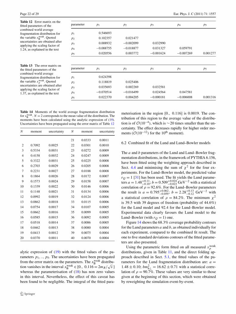
Page 22 of 29 Eur. Phys. J. C (2011) 71: 1557

Table 12 Error matrix on thefitted parameters of thecombined world averagefragmentation distribution forthe variable xweak

B . Quoteduncertainties are obtained afterapplying the scaling factor of1.24, as explained in the text

parameter p1 p2 p3 p4 p5

p1 0.546693

p2 0.102357 0.021477

p3 0.008932 −0.002099 0.032990

p4 −0.088755 −0.018877 0.031327 0.059791

p5 0.020556 0.003772 −0.001624 −0.007269 0.001277

Table 13 The error matrix onthe fitted parameters of thecombined world averagefragmentation distribution forthe variable xweak

p . Quoteduncertainties are obtained afterapplying the scaling factor of1.37, as explained in the text

parameter p1 p2 p3 p4 p5

p1 0.624398

p2 0.118819 0.025406

p3 0.035693 0.002269 0.032581

p4 −0.070514 −0.016499 0.024564 0.047581

p5 0.022370 0.004205 −0.000181 −0.006008 0.001316

Table 14 Moments of the world average fragmentation distributionfor xweak

B . N = 2 corresponds to the mean value of the distribution. Themoments have been calculated using the analytic expression of (19).Uncertainties have been propagated using the error matrix of Table 12

N moment uncertainty N moment uncertainty

21 0.0333 0.0011

2 0.7092 0.0025 22 0.0301 0.0010

3 0.5334 0.0031 23 0.0272 0.0009

4 0.4158 0.0032 24 0.0247 0.0009

5 0.3322 0.0031 25 0.0225 0.0008

6 0.2703 0.0029 26 0.0205 0.0008

7 0.2231 0.0027 27 0.0188 0.0008

8 0.1864 0.0026 28 0.0172 0.0007

9 0.1573 0.0024 29 0.0158 0.0007

10 0.1339 0.0022 30 0.0146 0.0006

11 0.1148 0.0021 31 0.0134 0.0006

12 0.0992 0.0019 32 0.0124 0.0006

13 0.0862 0.0018 33 0.0115 0.0006

14 0.0754 0.0017 34 0.0107 0.0005

15 0.0662 0.0016 35 0.0099 0.0005

16 0.0585 0.0015 36 0.0092 0.0005

17 0.0518 0.0014 37 0.0086 0.0005

18 0.0462 0.0013 38 0.0080 0.0004

19 0.0413 0.0012 39 0.0075 0.0004

20 0.0370 0.0011 40 0.0070 0.0004

alytic expression of (19) with the fitted values of the pa-rameters p1, ..,p5. The uncertainties have been propagatedfrom the error matrix on the parameters. The xweak

B distribu-tion vanishes in the interval xweak

B ∈ [0., 0.116 = 2mB/√

s ]whereas the parameterisation of (18) has non zero valuesin this interval. Nevertheless, the effect of this caveat hasbeen found to be negligible. The integral of the fitted para-

meterisation in the region [0., 0.116] is 0.0019. The con-tribution of this region to the average value of the distribu-tion is of O(10−4), which is ∼20 times smaller than the un-certainty. The effect decreases rapidly for higher order mo-ments (O(10−12) for the 10th moment).

6.2 Combined fit of the Lund and Lund–Bowler models

The a and b parameters of the Lund and Lund–Bowler frag-mentation distributions, in the framework of PYTHIA 6.156,have been fitted using the weighting approach described inSect. 4.4 and minimising the sum of χ2 for the four ex-periments. For the Lund–Bowler model, the predicted valuerQ = 1 [31] has been used. The fit yields the Lund parame-ters a = 1.48+0.11

−0.10; b = 0.509+0.024−0.023 GeV−2 with a statistical

correlation of ρ = 92.6%. For the Lund–Bowler parametersthe result is a = 0.795+0.062

−0.059; b = 2.28+0.13−0.12 GeV−2 with

a statistical correlation of ρ = 84.2%. The minimum χ2

is 39.5 with 39 degrees of freedom (probability of 44.6%)for the Lund model and 92.4 for the Lund–Bowler model.Experimental data clearly favours the Lund model to theLund–Bowler (with rQ = 1) one.

Figure 14 shows the 68.3% coverage probability contoursfor the Lund parameters a and b, as obtained individually foreach experiment, compared to the combined fit result. Theone to five standard deviations contours of the fitted parame-ters are also presented.

Using the parametric form fitted on all measured xweakp

distributions, given in Table 11, and the direct folding ap-proach described in Sect. 5.1, the fitted values of the pa-rameters for the Lund fragmentation distribution are: a =1.48 ± 0.10; bm2

b⊥ = 16.62 ± 0.71 with a statistical corre-lation of ρ = 90.7%. These values are very similar to thosegiven at the beginning of this section, which were obtainedby reweighting the simulation event-by-event.

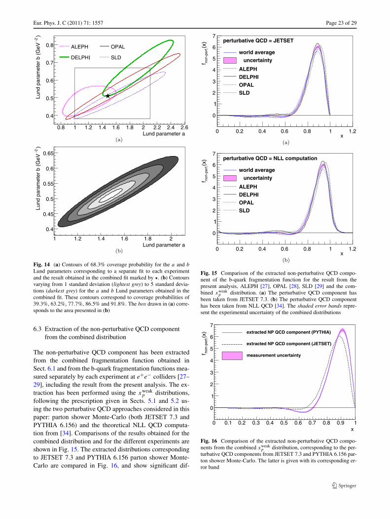
Eur. Phys. J. C (2011) 71: 1557 Page 23 of 29

Fig. 14 (a) Contours of 68.3% coverage probability for the a and b

Lund parameters corresponding to a separate fit to each experimentand the result obtained in the combined fit marked by �. (b) Contoursvarying from 1 standard deviation (lightest grey) to 5 standard devia-tions (darkest grey) for the a and b Lund parameters obtained in thecombined fit. These contours correspond to coverage probabilities of39.3%, 63.2%, 77.7%, 86.5% and 91.8%. The box drawn in (a) corre-sponds to the area presented in (b)

6.3 Extraction of the non-perturbative QCD componentfrom the combined distribution

The non-perturbative QCD component has been extractedfrom the combined fragmentation function obtained inSect. 6.1 and from the b-quark fragmentation functions mea-sured separately by each experiment at e+e− colliders [27–29], including the result from the present analysis. The ex-traction has been performed using the xweak

p distributions,following the prescription given in Sects. 5.1 and 5.2 us-ing the two perturbative QCD approaches considered in thispaper: parton shower Monte-Carlo (both JETSET 7.3 andPYTHIA 6.156) and the theoretical NLL QCD computa-tion from [34]. Comparisons of the results obtained for thecombined distribution and for the different experiments areshown in Fig. 15. The extracted distributions correspondingto JETSET 7.3 and PYTHIA 6.156 parton shower Monte-Carlo are compared in Fig. 16, and show significant dif-

Fig. 15 Comparison of the extracted non-perturbative QCD compo-nent of the b-quark fragmentation function for the result from thepresent analysis, ALEPH [27], OPAL [28], SLD [29] and the com-bined xweak

p distribution. (a) The perturbative QCD component hasbeen taken from JETSET 7.3. (b) The perturbative QCD componenthas been taken from NLL QCD [34]. The shaded error bands repre-sent the experimental uncertainty of the combined distributions

Fig. 16 Comparison of the extracted non-perturbative QCD compo-nents from the combined xweak

p distribution, corresponding to the per-turbative QCD components from JETSET 7.3 and PYTHIA 6.156 par-ton shower Monte-Carlo. The latter is given with its corresponding er-ror band

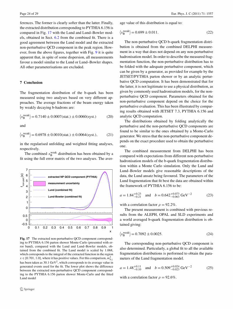
Page 24 of 29 Eur. Phys. J. C (2011) 71: 1557

ferences. The former is clearly softer than the latter. Finally,the extracted distribution corresponding to PYTHIA 6.156 iscompared in Fig. 17 with the Lund and Lund–Bowler mod-els, obtained in Sect. 6.2 from the combined fit. There is agood agreement between the Lund model and the extractednon-perturbative QCD component in the peak region. How-ever, from the above figures, together with Fig. 9 it is quiteapparent that, in spite of some dispersion, all measurementsfavour a model similar to the Lund or Lund–Bowler shapes.All other parameterisations are excluded.

7 Conclusion

The fragmentation distribution of the b-quark has beenmeasured using two analyses based on very different ap-proaches. The average fractions of the beam energy takenby weakly decaying b-hadrons are:

⟨xweak

B

⟩ = 0.7140 ± 0.0007(stat.) ± 0.0060(syst.) (20)

and

⟨xweak

B

⟩ = 0.6978 ± 0.0010(stat.) ± 0.0064(syst.), (21)

in the regularised unfolding and weighted fitting analyses,respectively.

The combined xweakB distribution has been obtained by a

fit using the full error matrix of the two analyses. The aver-

Fig. 17 The extracted non-perturbative QCD component correspond-ing to PYTHIA 6.156 parton shower Monte-Carlo (presented with er-ror band), compared with the Lund and Lund–Bowler models, ob-tained from the combined fit. The Lund model is scaled by 1.068,which corresponds to the integral of the extracted function in the regionx ∈ [0.701,1.0], where it has positive values. For this comparison, m2

b⊥has been taken as 30.1 GeV2, which corresponds to its average value ingenerated events used for the fit. The lower plot shows the differencebetween the extracted non-perturbative QCD component correspond-ing to the PYTHIA 6.156 parton shower Monte-Carlo and the fittedLund model

age value of this distribution is equal to:

⟨xweak

B

⟩ = 0.699 ± 0.011. (22)

The non-perturbative QCD b-quark fragmentation distri-bution is obtained from the combined DELPHI measure-ment in a way that does not depend on any non-perturbativehadronisation model. In order to describe the measured frag-mentation function, the non-perturbative distribution has tobe folded with the adequate perturbative component, whichcan be given by a generator, as provided for example by theJETSET/PYTHIA parton shower or by an analytic pertur-bative QCD computation. It has been demonstrated that forthe latter, it is not legitimate to use a physical distribution, asgiven by commonly used hadronisation models, for the non-perturbative QCD component. Parameters obtained for thenon-perturbative component depend on the choice for theperturbative evaluation. This has been illustrated by compar-ing results obtained with JETSET 7.3, PYTHIA 6.156 andanalytic QCD computation.

The distributions obtained by folding analytically theperturbative and the non-perturbative QCD components arefound to be similar to the ones obtained by a Monte-Carlogenerator. We stress that the non-perturbative component de-pends on the exact procedure used to obtain the perturbativeone.

The combined measurement from DELPHI has beencompared with expectations from different non-perturbativehadronisation models of the b-quark fragmentation distribu-tion within a Monte Carlo simulation. Only the Lund andLund–Bowler models give reasonable descriptions of thedata, the Lund ansatz being favoured. The parameters of theLund fragmentation that fit best the data are obtained withinthe framework of PYTHIA 6.156 to be:

a = 1.84+0.23−0.21 and b = 0.642+0.073

−0.063 GeV−2 (23)

with a correlation factor ρ = 92.2%.The present measurement is combined with previous re-

sults from the ALEPH, OPAL and SLD experiments anda world averaged b-quark fragmentation distribution is ob-tained giving:

⟨xweak

B

⟩ = 0.7092 ± 0.0025. (24)

The corresponding non-perturbative QCD component isalso determined. Particularly, a global fit to all the availablefragmentation distributions is performed to obtain the para-meters of the Lund fragmentation model.

a = 1.48+0.11−0.10 and b = 0.509+0.024

−0.023 GeV−2 (25)

with a correlation factor ρ = 92.6%.

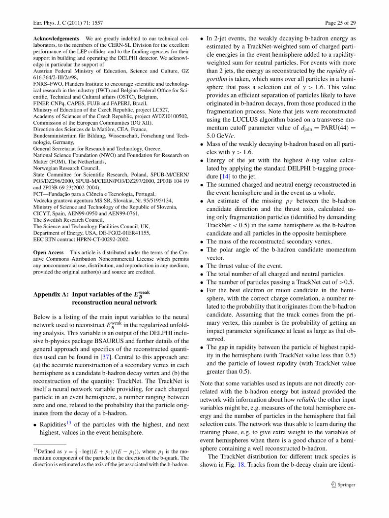
Eur. Phys. J. C (2011) 71: 1557 Page 25 of 29

Acknowledgements We are greatly indebted to our technical col-laborators, to the members of the CERN-SL Division for the excellentperformance of the LEP collider, and to the funding agencies for theirsupport in building and operating the DELPHI detector. We acknowl-edge in particular the support ofAustrian Federal Ministry of Education, Science and Culture, GZ616.364/2-III/2a/98,FNRS–FWO, Flanders Institute to encourage scientific and technolog-ical research in the industry (IWT) and Belgian Federal Office for Sci-entific, Technical and Cultural affairs (OSTC), Belgium,FINEP, CNPq, CAPES, FUJB and FAPERJ, Brazil,Ministry of Education of the Czech Republic, project LC527,Academy of Sciences of the Czech Republic, project AV0Z10100502,Commission of the European Communities (DG XII),Direction des Sciences de la Matiere, CEA, France,Bundesministerium fur Bildung, Wissenschaft, Forschung und Tech-nologie, Germany,General Secretariat for Research and Technology, Greece,National Science Foundation (NWO) and Foundation for Research onMatter (FOM), The Netherlands,Norwegian Research Council,State Committee for Scientific Research, Poland, SPUB-M/CERN/PO3/DZ296/2000, SPUB-M/CERN/PO3/DZ297/2000, 2P03B 104 19and 2P03B 69 23(2002-2004),FCT—Fundação para a Ciência e Tecnologia, Portugal,Vedecka grantova agentura MS SR, Slovakia, Nr. 95/5195/134,Ministry of Science and Technology of the Republic of Slovenia,CICYT, Spain, AEN99-0950 and AEN99-0761,The Swedish Research Council,The Science and Technology Facilities Council, UK,Department of Energy, USA, DE-FG02-01ER41155,EEC RTN contract HPRN-CT-00292-2002.

Open Access This article is distributed under the terms of the Cre-ative Commons Attribution Noncommercial License which permitsany noncommercial use, distribution, and reproduction in any medium,provided the original author(s) and source are credited.

Appendix A: Input variables of the EweakB

reconstruction neural network

Below is a listing of the main input variables to the neuralnetwork used to reconstruct Eweak

B in the regularized unfold-ing analysis. This variable is an output of the DELPHI inclu-sive b-physics package BSAURUS and further details of thegeneral approach and specifics of the reconstructed quanti-ties used can be found in [37]. Central to this approach are:(a) the accurate reconstruction of a secondary vertex in eachhemisphere as a candidate b-hadron decay vertex and (b) thereconstruction of the quantity: TrackNet. The TrackNet isitself a neural network variable providing, for each chargedparticle in an event hemisphere, a number ranging betweenzero and one, related to the probability that the particle orig-inates from the decay of a b-hadron.

• Rapidities13 of the particles with the highest, and nexthighest, values in the event hemisphere.

13Defined as y = 12 · log((E + p‖)/(E − p‖)), where p‖ is the mo-

mentum component of the particle in the direction of the b-quark. Thedirection is estimated as the axis of the jet associated with the b-hadron.

• In 2-jet events, the weakly decaying b-hadron energy asestimated by a TrackNet-weighted sum of charged parti-cle energies in the event hemisphere added to a rapidity-weighted sum for neutral particles. For events with morethan 2 jets, the energy as reconstructed by the rapidity al-gorithm is taken, which sums over all particles in a hemi-sphere that pass a selection cut of y > 1.6. This valueprovides an efficient separation of particles likely to haveoriginated in b-hadron decays, from those produced in thefragmentation process. Note that jets were reconstructedusing the LUCLUS algorithm based on a transverse mo-mentum cutoff parameter value of djoin = PARU(44) =5.0 GeV/c.

• Mass of the weakly decaying b-hadron based on all parti-cles with y > 1.6.

• Energy of the jet with the highest b-tag value calcu-lated by applying the standard DELPHI b-tagging proce-dure [14] to the jet.

• The summed charged and neutral energy reconstructed inthe event hemisphere and in the event as a whole.

• An estimate of the missing pT between the b-hadroncandidate direction and the thrust axis, calculated us-ing only fragmentation particles (identified by demandingTrackNet < 0.5) in the same hemisphere as the b-hadroncandidate and all particles in the opposite hemisphere.

• The mass of the reconstructed secondary vertex.• The polar angle of the b-hadron candidate momentum

vector.• The thrust value of the event.• The total number of all charged and neutral particles.• The number of particles passing a TrackNet cut of >0.5.• For the best electron or muon candidate in the hemi-

sphere, with the correct charge correlation, a number re-lated to the probability that it originates from the b-hadroncandidate. Assuming that the track comes from the pri-mary vertex, this number is the probability of getting animpact parameter significance at least as large as that ob-served.

• The gap in rapidity between the particle of highest rapid-ity in the hemisphere (with TrackNet value less than 0.5)and the particle of lowest rapidity (with TrackNet valuegreater than 0.5).

Note that some variables used as inputs are not directly cor-related with the b-hadron energy but instead provided thenetwork with information about how reliable the other inputvariables might be, e.g. measures of the total hemisphere en-ergy and the number of particles in the hemisphere that failselection cuts. The network was thus able to learn during thetraining phase, e.g. to give extra weight to the variables ofevent hemispheres when there is a good chance of a hemi-sphere containing a well reconstructed b-hadron.

The TrackNet distribution for different track species isshown in Fig. 18. Tracks from the b-decay chain are identi-

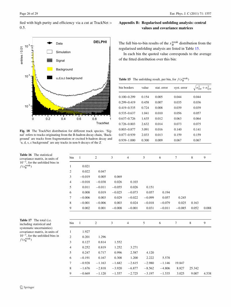
Page 26 of 29 Eur. Phys. J. C (2011) 71: 1557

fied with high purity and efficiency via a cut at TrackNet >

0.5.

Fig. 18 The TrackNet distribution for different track species. ‘Sig-nal’ refers to tracks originating from the B-hadron decay chain, ‘Back-ground’ are tracks from fragmentation or excited b-hadron decay and‘u, d, s, c background’ are any tracks in non-b decays of the Z

Appendix B: Regularised unfolding analysis: centralvalues and covariance matrices

The full bin-to-bin results of the xweakB distribution from the

regularised unfolding analysis are listed in Table 15.In each bin the quoted value corresponds to the average

of the fitted distribution over this bin:

Table 15 The unfolding result, per bin, for f (xweakB )

bin borders value stat. error syst. error√

σ 2stat + σ 2

syst

0.100–0.299 0.154 0.005 0.044 0.044

0.299–0.419 0.458 0.007 0.035 0.036

0.419–0.535 0.724 0.008 0.039 0.039

0.535–0.637 1.041 0.010 0.056 0.057

0.637–0.726 1.635 0.012 0.063 0.064

0.726–0.803 2.632 0.014 0.073 0.075

0.803–0.877 3.091 0.016 0.140 0.141

0.877–0.939 2.033 0.013 0.159 0.159

0.939–1.000 0.300 0.009 0.067 0.067

Table 16 The statisticalcovariance matrix, in units of10−3, for the unfolded bins inf (xweak

B )

bin 1 2 3 4 5 6 7 8 9

1 0.021

2 0.022 0.047

3 −0.019 0.005 0.069

4 −0.018 −0.038 0.026 0.103

5 0.011 −0.011 −0.055 0.026 0.151

6 0.008 0.019 −0.025 −0.073 0.057 0.194

7 −0.006 0.003 0.029 −0.022 −0.099 0.057 0.245

8 −0.001 −0.006 0.003 0.024 −0.018 −0.079 0.025 0.163

9 0.002 0.001 −0.008 −0.001 0.031 −0.011 −0.085 0.052 0.088

Table 17 The total (i.e.including statistical andsystematic uncertainties)covariance matrix, in units of10−3, for the unfolded bins inf (xweak

B )

bin 1 2 3 4 5 6 7 8 9

1 1.927

2 0.201 1.296

3 0.127 0.814 1.552

4 0.252 0.819 1.252 3.271

5 0.247 0.717 0.996 2.587 4.120

6 −0.191 0.167 0.308 1.200 2.222 5.578

7 −0.928 −1.163 −1.682 −2.615 −2.980 −1.146 19.847

8 −1.676 −2.818 −3.920 −6.877 −8.562 −4.806 8.827 25.342

9 −0.669 −1.120 −1.557 −2.725 −3.197 −1.535 3.025 9.007 4.538

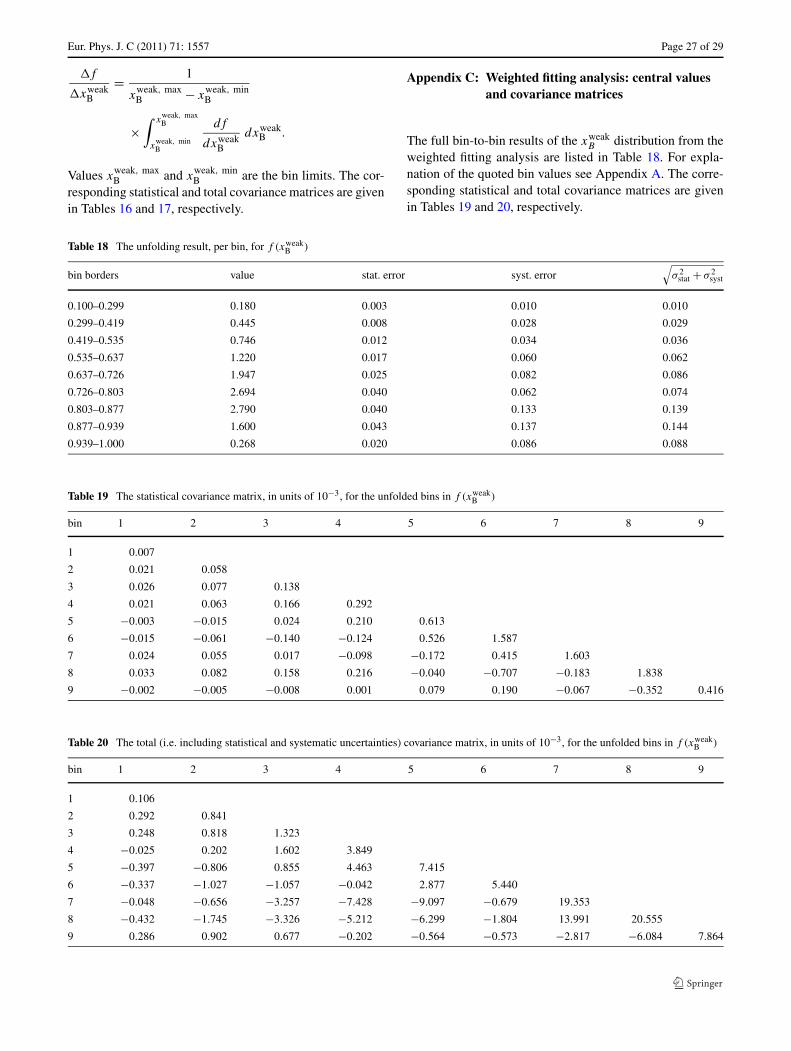
Eur. Phys. J. C (2011) 71: 1557 Page 27 of 29

f

xweakB

= 1

xweak, maxB − x

weak, minB

×∫ x

weak, maxB

xweak, minB

df

dxweakB

dxweakB .

Values xweak, maxB and x

weak, minB are the bin limits. The cor-

responding statistical and total covariance matrices are givenin Tables 16 and 17, respectively.

Table 18 The unfolding result, per bin, for f (xweakB )

bin borders value stat. error syst. error√

σ 2stat + σ 2

syst

0.100–0.299 0.180 0.003 0.010 0.010

0.299–0.419 0.445 0.008 0.028 0.029

0.419–0.535 0.746 0.012 0.034 0.036

0.535–0.637 1.220 0.017 0.060 0.062

0.637–0.726 1.947 0.025 0.082 0.086

0.726–0.803 2.694 0.040 0.062 0.074

0.803–0.877 2.790 0.040 0.133 0.139

0.877–0.939 1.600 0.043 0.137 0.144

0.939–1.000 0.268 0.020 0.086 0.088

Table 19 The statistical covariance matrix, in units of 10−3, for the unfolded bins in f (xweakB )

bin 1 2 3 4 5 6 7 8 9

1 0.007

2 0.021 0.058

3 0.026 0.077 0.138

4 0.021 0.063 0.166 0.292

5 −0.003 −0.015 0.024 0.210 0.613

6 −0.015 −0.061 −0.140 −0.124 0.526 1.587

7 0.024 0.055 0.017 −0.098 −0.172 0.415 1.603

8 0.033 0.082 0.158 0.216 −0.040 −0.707 −0.183 1.838

9 −0.002 −0.005 −0.008 0.001 0.079 0.190 −0.067 −0.352 0.416

Table 20 The total (i.e. including statistical and systematic uncertainties) covariance matrix, in units of 10−3, for the unfolded bins in f (xweakB )

bin 1 2 3 4 5 6 7 8 9

1 0.106

2 0.292 0.841

3 0.248 0.818 1.323

4 −0.025 0.202 1.602 3.849

5 −0.397 −0.806 0.855 4.463 7.415

6 −0.337 −1.027 −1.057 −0.042 2.877 5.440

7 −0.048 −0.656 −3.257 −7.428 −9.097 −0.679 19.353

8 −0.432 −1.745 −3.326 −5.212 −6.299 −1.804 13.991 20.555

9 0.286 0.902 0.677 −0.202 −0.564 −0.573 −2.817 −6.084 7.864

Appendix C: Weighted fitting analysis: central valuesand covariance matrices

The full bin-to-bin results of the xweakB distribution from the

weighted fitting analysis are listed in Table 18. For expla-nation of the quoted bin values see Appendix A. The corre-sponding statistical and total covariance matrices are givenin Tables 19 and 20, respectively.

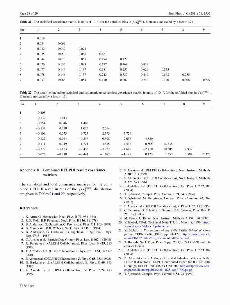
Page 28 of 29 Eur. Phys. J. C (2011) 71: 1557

Table 21 The statistical covariance matrix, in units of 10−3, for the unfolded bins in f (xweakB ). Elements are scaled by a factor 1.71

bin 1 2 3 4 5 6 7 8 9

1 0.019

2 0.034 0.069

3 0.022 0.049 0.072

4 0.025 0.050 0.086 0.181

5 0.044 0.078 0.061 0.194 0.422

6 0.076 0.133 0.098 0.177 0.468 0.819

7 0.077 0.144 0.137 0.181 0.257 0.629 0.833

8 0.078 0.146 0.137 0.243 0.337 0.449 0.568 0.755

9 0.037 0.063 0.054 0.110 0.207 0.240 0.140 0.308 0.227

Table 22 The total (i.e. including statistical and systematic uncertainties) covariance matrix, in units of 10−3, for the unfolded bins in f (xweakB ).

Elements are scaled by a factor 1.71

bin 1 2 3 4 5 6 7 8 9

1 0.408

2 −0.139 1.013

3 0.554 0.346 1.403

4 −0.134 0.730 1.013 2.514

5 −0.109 0.073 0.723 2.393 3.729

6 −0.122 0.044 −0.216 0.398 2.056 4.850

7 −0.111 −0.319 −1.721 −3.815 −4.596 −0.505 14.838

8 −0.372 −1.123 −2.413 −3.922 −4.605 −2.410 10.305 14.939

9 0.075 −0.210 −0.441 −1.102 −1.149 0.123 1.550 3.507 2.373

Appendix D: Combined DELPHI result: covariancematrices

The statistical and total covariance matrices for the com-bined DELPHI result in bins of the f (xweak

B ) distributionare given in Tables 21 and 22, respectively.

References

1. X. Artru, G. Mennessier, Nucl. Phys. B 70, 93 (1974)2. R.D. Field, R.P. Feynman, Nucl. Phys. B 136, 1 (1978)3. B. Andersson, G. Gustafson, C. Peterson, Z. Phys. C 1, 105 (1979)4. G. Marchesini, B.R. Webber, Nucl. Phys. B 238, 1 (1984)5. B. Andersson, G. Gustafson, G. Ingelman, T. Sjöstrand, Phys.

Rep. 97, 31 (1983)6. C. Amsler et al. (Particle Data Group), Phys. Lett. B 667, 1 (2008)7. R. Barate et al. (ALEPH Collaboration), Phys. Lett. B 425, 215

(1998)8. T. Affolder et al. (CDF Collaboration), Phys. Rev. D 64, 072002

(2001)9. P. Abreu et al. (DELPHI Collaboration), Z. Phys. C 68, 353 (1995)

10. D. Buskulic et al. (ALEPH Collaboration), Z. Phys. C 69, 393(1996)

11. K. Akerstaff et al. (OPAL Collaboration), Z. Phys. C 74, 413(1997)

12. P. Aarnio et al. (DELPHI Collaboration), Nucl. Instrum. MethodsA 303, 233 (1991)

13. P. Abreu et al. (DELPHI Collaboration), Nucl. Instrum. MethodsA 378, 57 (1996)

14. J. Abdallah et al. (DELPHI Collaboration), Eur. Phys. J. C 32, 185(2004)

15. T. Sjöstrand, Comput. Phys. Commun. 39, 347 (1986)16. T. Sjöstrand, M. Bengtsson, Comput. Phys. Commun. 43, 367

(1987)17. P. Abreu et al. (DELPHI Collaboration), Z. Phys. C 73, 11 (1996)18. C. Peterson, D. Schlatter, I. Schmitt, P.M. Zerwas, Phys. Rev. D

27, 105 (1983)19. M. Feindt, U. Kerzel, Nucl. Instrum. Methods A 559, 190 (2006)20. V. Blobel, OPAL Technical Note TN361, March 8, 1996. http://

www.desy.de/~blobel/opalnote.ps21. V. Blobel, in Proceedings of the 1984 CERN School of Com-

puting, CERN 85-09 (1985), pp. 88–127. http://cdsweb.cern.ch/record/161223/files/full_document.pdf?version=1

22. T. Boccali, Nucl. Phys. Proc. Suppl. 75B(3), 241 (1999) and ref-erences therein

23. J. Abdallah et al. (DELPHI Collaboration), Eur. Phys. J. C 33, 307(2004)

24. Z. Albrecht et al., A study of excited b-hadron states with theDELPHI detector at LEP1, Contributed Paper for ICHEP 2004(Beijing), DELPHI 2004-025 CONF 700. http://delphiwww.cern.ch/pubxx/delnote/public/2004_025_conf_700.ps.gz

25. T. Sjöstrand, Comput. Phys. Commun. 82, 74 (1994)

Eur. Phys. J. C (2011) 71: 1557 Page 29 of 29

26. P. Abreu et al. (DELPHI Collaboration), Phys. Lett. B 462, 425(1999)

27. A. Heister et al. (ALEPH Collaboration), Phys. Lett. B 512, 30(2001)

28. G. Abbiendi et al. (OPAL Collaboration), Eur. Phys. J. C 29, 463(2003)

29. K. Abe et al. (SLD Collaboration), Phys. Rev. D 65, 092006(2002). Erratum-ibid. 66, 079905 (2002)

30. B. Andersson, G. Gustafson, B. Soderberg, Z. Phys. C 20, 317(1983)

31. M.G. Bowler, Z. Phys. C 11, 169 (1981)

32. E. Ben-Haim, FERMILAB-THESIS-2004-50. http://publication.lal.in2p3.fr/2004/lal04124.pdf

33. E. Ben-Haim, P. Bambade, P. Roudeau, A. Savoy-Navarro,A. Stocchi, Phys. Lett. B 580, 108 (2004)

34. M. Cacciari, S. Catani, Nucl. Phys. B 617, 253 (2001)35. V.G. Kartvelishvili, A.K. Likehoded, V.A. Petrov, Phys. Lett. B

78, 615 (1978)36. P. Collins, T. Spiller, J. Phys. G 11, 1289 (1985)37. Z. Albrecht, T. Allmendinger, G.J. Barker, M. Feindt, C. Haag,

M. Moch, hep-ex/0102001