INTERNATIONAL JOURNAL OF CLIMATOLOGYInt. J. Climatol. (2014)Published online in Wiley Online Library(wileyonlinelibrary.com) DOI: 10.1002/joc.4218

A study of the air–sea interaction in the South AtlanticConvergence Zone through Granger causality

Giulio Tirabassi,a* Cristina Masollera and Marcelo Barreirob

a Universitat Politecnica de Catalunya, Terrassa, Spainb Departamento de Ciencias de la Atmosfera, Instituto de Fisica, Universidad de la Republica, Montevideo, Uruguay

ABSTRACT: Air–sea interaction in the region of the South Atlantic Convergence Zone (SACZ) is studied using Grangercausality (GC) as a measure of directional coupling. Calculation of the area weighted connectivity indicates that the SACZregion is the one with largest mutual air–sea connectivity in the south Atlantic basin during summertime. Focusing on theleading mode of daily coupled variability, GC allows distinguishing four regimes characterized by different coupling: thereare years in which the forcing is mainly directed from the atmosphere to the ocean, years in which the ocean forces theatmosphere, years in which the influence is mutual and years in which the coupling is not significant. A composite analysisshows that ocean-driven events have atmospheric anomalies that develop first and are strongest over the ocean, while in eventswithout coupling anomalies develop from the continent where they are strongest and have smaller oceanic extension.

KEY WORDS air–sea interactions; SACZ; Granger causality; climate network

Received 21 February 2014; Revised 20 October 2014; Accepted 28 October 2014

1. Introduction

The South Atlantic Convergence Zone (SACZ) is one ofthe main components of the South American Monsoon: itis a convective pattern that extends from the Amazon forestto the subtropical South Atlantic Ocean (SAO), orientedin northwest–southeast direction (Carvalho et al., 2002,2004; Bombardi et al., 2013). When active, the SACZ isassociated with heavy precipitation over the Amazon for-est and southeastern Brazil, causing floods and landslidesover the densely populated areas of Minas Gerais, SaoPaulo and Rio de Janeiro.

The main mode of SACZ variability consists of a pre-cipitation dipole with centres over the SACZ and overUruguay, such that when the SACZ is active there isdecreased rainfall over Uruguay and vice versa. This modevaries on several time scales ranging from day-to-day,due to the passage of fronts, to intraseasonal, interan-nual and even longer time scales having been associ-ated with the observed summertime rainfall trend in east-ern South America during the 20th century (Kodama,1992; Nogués-Paegle and Mo, 1997; Barreiro et al., 2002;Junquas et al., 2012).

Due to its socio-economic importance, there have beenseveral attempts to improve our understanding and pre-dictability of rainfall over the SACZ on seasonal to interan-nual time scales, particularly focusing on the role of upperocean in modulating its behaviour. Studies have shownthat the subtropical SAO may influence the evolution of

* Correspondence to: G. Tirabassi, Universitat Politecnica de Catalunya,Terrassa, Spain. E-mail: giulio.tirabassi@upc.edu

the SACZ (Robertson and Mechoso, 2000; Barreiro et al.,2002, 2005). For example, Barreiro et al. (2002, 2005)show that even though the region is dominated by inter-nal atmospheric variability, sea surface temperature (SST)anomalies can force a dipole of precipitation anomalieslocated mainly over the oceanic portion of the SACZ. Sub-sequent studies have suggested that the air–sea interactionis such that an initially stronger SACZ – due to inter-nal atmospheric variability – induces an oceanic coolingthat in turn negatively affects the convective precipitation,resulting in a negative feedback loop (Chaves and Nobre,2004; De Almeida et al., 2007).

However, air–sea interaction has been difficult to quan-tify both in observations and in model simulations and todate it is unclear how the circulation associated with theSACZ is influenced by surface ocean conditions. Disentan-gling air–sea interaction in the subtropics is a challengingtask, and up to now to the best of our knowledge, nomethod has allowed a robust identification of this inter-action in observational data. To tackle this problem, wepropose a new methodology based on the combined useof Granger causality (GC) together with a new measurefrom climate network theory (area weighted connectiv-ity, AWC) and maximum covariance analysis (MCA);this methodology aims to assess the presence of air–seainteraction, and to distinguish among different interactionregimes.

We find that for the leading SACZ mode of variabilitythe air–sea coupling is significantly active only in 50% ofthe cases, and that when active, it manifests itself in threedistinct ‘flavours’: there are years in which the forcing ismainly directed from the atmosphere to the ocean, years

© 2014 Royal Meteorological Society

G. TIRABASSI et al.

in which the ocean forces the atmosphere and years inwhich the influence is mutual. Moreover, we find that theconditions in the upper ocean can modulate rainfall eventsin the SACZ, affecting the position, the intensity and thepersistence of the precipitation anomalies.

2. Data

As a proxy for precipitation, we consider the vertical veloc-ity at 500 hPa, 𝜔, while the ocean state is characterized bythe SST. Both data sets are daily mean data provided byERA INTERIM reanalysis (Dee et al., 2011), ranging fromDecember 1979 to March 2013 on a horizontal grid with1.5 degrees of resolution. We restricted the analysis to aus-tral summer months (December–March) when the SACZshows strongest activity. Anomalies were calculated firstremoving the annual cycle by subtracting the average valuefor each day, and then normalizing the series to have unitvariance.

3. The GC estimator

We assume that the time series at each grid point can bedescribed by a D-dimensional autoregressive process in theform (Mosedale et al., 2006)

Yt =D∑

k=1

akYt−k +D∑

k=1

bkXt−k + 𝜀t (1)

where X is the forcing and Y the slave variable. Here akand bk are vectors of coefficients and 𝜀 are the associatedresiduals. Y is either SST or vertical velocity (𝜔) at acertain location (but not necessarily the same): if Y =SST,then X =𝜔 and vice versa. Considering two time series atdifferent locations allows analysing non-local air–oceaninteractions.

We apply to this autoregressive model a GC test: the firststep of this procedure is to fit ak and bk with a linear regres-sion, and compute the associated variance of the residuals,𝜎

2coupled. In the second step, the fit is repeated setting bk = 0,

and again the variance of the residuals is computed, namely𝜎

2uncoupled. The last step involves comparing the two resid-

ual variances: if the variance in the coupled case is smallerthan the one computed in the uncoupled one, it meansthat the predictive power of the coupled model is higher,and thus, X is Granger causal of Y . In other words, X isGranger causal of Y if X helps predict Y at some time inthe future. Then, the prediction improvement is measuredby the Granger causality estimator (GCE) as in Mokhovet al. (2011).

GCE =𝜎

2uncoupled − 𝜎

2coupled

𝜎2uncoupled

(2)

We tested the significance of the GCE value with a F-test.X is considered a true Granger causal of Y only if theassociated GCE value is significant at a certain confidencelevel (as explained below, we used 99% confidence level

and 90%, depending on the available statistics). If X isGranger causal of Y , we will denote this fact as X → Y . Ifalso Y is Granger causal of X, thus forming a closed-loopsystem, the notation X ↔ Y will be used instead.

Finally, the dimension of the autoregressive model D, forevery time series Y of length T days, is chosen in order tominimize the function,

S (D) = T2

ln

(𝜎

2uncoupled

𝜎2Y

)+ D

2ln (T) (3)

that is a good compromise between obtaining a good fittingand avoiding over-fitting (Schwarz, 1978). Typical valuesof D are about 8 days for SST and 4 days for 𝜔, dependingon the location.

GC is a powerful tool for the analysis of climatetime series (Stern and Kaufmann, 1999, 2014; Salvucciet al., 2002; Khokhlov et al., 2006; Mosedale et al., 2006;Mokhov et al., 2011; Attanasio et al., 2012; Pasini et al.,2012). It is especially useful in systems that exhibit feed-back and closed loops, for which the lagged correla-tion can lead to misleading conclusions (Chatfield, 1989;Runge et al., 2014). Note, however, that this methodologycan detect linear dependencies only and assumes that thetime series are covariance stationary. A drawback of themethodology is that if X and Y are strongly influenced bya third unknown factor, the method could find that X isGranger causal of Y even though the real causality is differ-ent. Throughout this work, we will consider that X forcesY if X is Granger causal of Y , bearing in mind the previousdrawback.

4. Air–sea connectivity

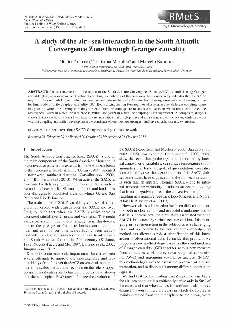
We start by focusing on the region [20N, 40S]× [70W,20E], and compute the GCE at each grid node, both inthe direction SST→𝜔 and 𝜔→ SST. In this way, we wantto estimate the local interaction between the two systems,i.e. the interaction between a grid point in the ocean andthe one placed in the atmosphere just above it. The GCEvalues at 99% confidence level are plotted in Figure 1. Asit can be observed in (a), the main two zones in which theocean forces the atmosphere are the deep tropics and thesubtropical waters off Brazil. The deep tropics is expectedto be a region of oceanic forcing (e.g. Hoskins and Karoly,1981), and the methodology consistently captures this fact.The ocean off southeast Brazil corresponds to the SACZregion and is within our region of interest. Moreover,Figure 1(b) clearly shows that the atmosphere stronglyforces the surface ocean also off Brazil. Thus, this oceanregion can play both an active and a passive role, providinga hint of the presence of complex feedback loops in the area(Chaves and Nobre, 2004; De Almeida et al., 2007).

As the atmosphere and the ocean interact on largerspatial scales – not only locally – the calculation of thelocal GCE value provides limited information. There-fore, we computed the cross-GCE, in which the GCEis evaluated, in the two directions, for every couple of

© 2014 Royal Meteorological Society Int. J. Climatol. (2014)

AIR–SEA INTERACTION IN THE SACZ THROUGH GRANGER CAUSALITY

Figure 1. Local GCE for SST→𝜔 (a) and 𝜔→SST (b). Only values significant at 99% confidence level are reported.

ocean–atmosphere nodes. In this way, we are investigatingalso the presence of non-local forcing.

To represent this result, we built a two-layer network(Tsonis and Roebber, 2004) based on significant GCEs:every node of the network is a grid point of the oceanicor of the atmospheric layer, and it is linked to points inthe other layer only if their GCE is significant at 99%confidence level. The resulting network is a bipartite one,i.e. a network composed of two set of nodes in which thereare links only from one set to the other. Furthermore, thoselinks are directed and allow for feedback loops.

An easy way to represent such a network is throughthe so-called adjacency matrix, A. The dimension of A isN ×N, where N is the number of grid points for each layer,and it is composed of only 0s and 1s. Namely, if two nodesi and j are connected, then Ai→j = 1 and it is 0 otherwise.As the GCE is a directional measure, A is a non-symmetricmatrix, i.e. Ai→j may be different from Aj→i. For example,a location i in the ocean can be forcing a point j in theatmosphere without being forced by j itself.

Using the adjacency matrix, we can compute the AWCfor the oceanic and the atmospheric layers. The AWC isdefined as follows (Tsonis and Roebber, 2004):

AWCi =

N∑j=1

Ai→j cos(𝜆j

)N∑

j=1

cos(𝜆j

) (4)

where i corresponds to the nodes in one layer, j to the nodesin the other layer, 𝜆j is the latitude of node j and N is thenumber of grid points in the studied region. The links wereweighted with cos(𝜆i) to correct the bias induced by thedifferent areas represented by the different grid points, as itis usually done in climate network analysis (Donges et al.,2009; Deza et al., 2013; Tirabassi and Masoller, 2013).

It is easy to see that the AWCi is the fraction of theregion under study to which a node i is connected to. Thus,nodes with high AWC correspond to points of one layerthat exercise a broad forcing on the other layer, and thisway, the AWC reveals to be a powerful way to quantify

the spatial ranges of interaction of the two systems. Inparticular, high values of AWC indicate points that havea significant GC with many other points in the other layer.However, the AWC does not provide information about theactual value of this GC. A very weak forcing but actingover a large area, in fact, has a high value of AWC buta very low value of local GCE, while a strong forcingacting over a very narrow area has a low AWC togetherwith a high local value of GCE. Note, however, that theAWC depends on the chosen region because atmosphericlong-range teleconnections, that extend beyond the regionconsidered, are not taken into account.

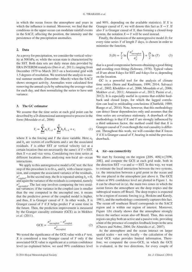
The AWC maps are depicted in Figure 2. The AWC mapassociated with SST→𝜔 forcing (Figure 2(a)) presentstwo maxima. The first one is on the equator, at about 20Wand is coincident with the tropical component of the map oflocal GCE. However, the largest AWC is placed offshorethe southern Brazil coast and corresponds to the secondmaximum in the map of local GCE (Figure 1(a)). Thus,the relative magnitude of the signal in the equatorial andsubtropical regions is opposed with respect to the localmeasure, suggesting that the SST forcing in the tropicsis stronger but mainly local (vertical), while in the SACZregion it is weaker but non-local. In fact, while in the deeptropical Atlantic we have small values of AWC and highvalues of local GCE, in the subtropical part of the ocean thesituation is the opposite, with many points presenting highAWC but relatively low values of GCE (low, comparedwith the tropical ones). This might be related to the factthat SST anomalies in the subtropics vary coherently ona larger spatial scale than in the equatorial Atlantic. Weremark that the GCE values used to build these maps arestatistically significant at 99% confidence level.

Regarding the AWC map of 𝜔→ SST (Figure 2(b)),the connectivity is generally large over the whole region,stressing the dominant role of atmospheric circulation inforcing SST anomalies. Moreover, there is a large highlyconnected region south of 30S, which corresponds to alargely non-local pattern of connectivity (we can see avery feeble signal in the local map in Figure 1(b)). Thelocation of the maximum suggests that it could be relatedto the influence of the south Atlantic anticyclone on SST

© 2014 Royal Meteorological Society Int. J. Climatol. (2014)

G. TIRABASSI et al.

Figure 2. AWC for GC-based bilayer climate network composed of SST and 𝜔 data sets. (a) AWC computed with SST→𝜔 GCE. (b) AWC computedvia 𝜔→ SST GCE. Only GCE values significant at 99% confidence level have been used to compute the AWC.

through, for example, wind-induced changes in latent heatfluxes.

Taken together, these maps reveal that the SACZ regiondisplays complex air–sea interactions in agreement withprevious studies, e.g. Carvalho et al. (2004) and DeAlmeida et al. (2007). Nonetheless, it is important tonote that the AWC maps provide information only aboutthe spatial range of the interactions but not about theirstrengths. Moreover, the 𝜔 field is very noisy includingseveral types of phenomena that need not be directlyrelated to the SACZ dynamics. Thus, in order to gain moreinsight about air–sea interactions in the region, the nextsection focuses on the leading mode of coupled variability.

5. Directionality of air–sea coupling

The leading mode of covariability between SST and 𝜔

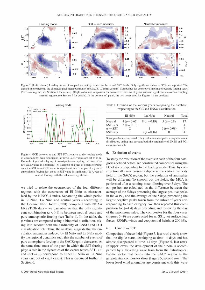
was computed using MCA (Bretherton et al. (1992)). Itexplains 8% of the cross covariance and is depicted inFigure 3, left column. It represents the intensification andnorthward shifting of the SACZ pattern with respect tothe climatology, accompanied by a cooling of the SST inbetween the two lobes of the dipole, with maximum cool-ing below increased convection. As mentioned in Section1, this dipole pattern has been shown to be the leadingmode of variability in the region on several time scales(Bombardi et al., 2013). Note that the region of oceancooling is consistent with the one displayed in the AWCand in local GCE maps in Figures 1 and 2. Moreover, themap of points connected to the region of maximum AWCoff Brazil reveals a structure consisting in two parallelbands oriented NW–SE, very similar in shape to Figure 3(not shown). This suggests that this mode represents abi-directional interaction of the two fields.

Focusing on the dynamics of the first mode, whichrepresents the SACZ variability, allows to filter a goodfraction of the weather noise and to truly concentrate on theinterannual variability of the SACZ. In particular, SACZevents will evolve differently depending on the air–seainteraction.

To find the direction of the coupling between the oceanicand atmospheric patterns in the leading mode, shown inFigure 3, we calculated the GCE using the correspond-ing principal components (PCs) over the whole period ofstudy. The similarity of the values obtained (0.019 in theSST→𝜔 direction and 0.021 in the 𝜔→ SST one, witha relative difference of less than 10%) indicates that theair–sea interaction is very important in this mode, and con-firms the results of the previous analysis, once again show-ing the presence of feedbacks between the atmosphere andthe subtropical south Atlantic. We stress that both thesevalues are significant at the 99% confidence level.

The second mode of covariability (7%), instead, showsthe imprint of the south Atlantic anticyclone, especially inthe SST component, suggesting that this is likely an atmo-spheric driven mode (not shown). This hypothesis wasconfirmed by the calculation of the GCE of the correspond-ing PCs (0.021 and 0.027, respectively), and the mode isnot studied further here.

We next calculated the GCE for every year of the PCs(Figure 4), which allowed to classify individual years intofour regimes: 𝜔 forcing SST (9 years) and SST forcing𝜔 (4 years) if only one GCE is statistically significant,double forcing (4 years) if both GCE values are significantand neutral (17 years) if no GCE value is significant at90% confidence level. The patterns associated with theSST forcing and neutral cases are shown in Figure 3. Inthe neutral case, SST anomalies are small and rainfallanomalies are strongest over land. In the SST forced case,on the contrary, there are large SST anomalies with adipolar structure and rainfall anomalies are largest overthe oceanic portion of the SACZ. Section 6 will study theevolution of these events.

From the analysis, it remains unclear whether the highnumber of neutral years is a consequence of the small num-ber of data that compose the annual data sets (4 months,i.e. 121 days), or indeed, there are no significant interac-tions between the atmosphere and ocean. The compositeanalysis presented below suggests the latter.

Considering that El Niño can significantly affect theSACZ region (Barreiro et al., 2002; Kayano et al., 2013),

© 2014 Royal Meteorological Society Int. J. Climatol. (2014)

AIR–SEA INTERACTION IN THE SACZ THROUGH GRANGER CAUSALITY

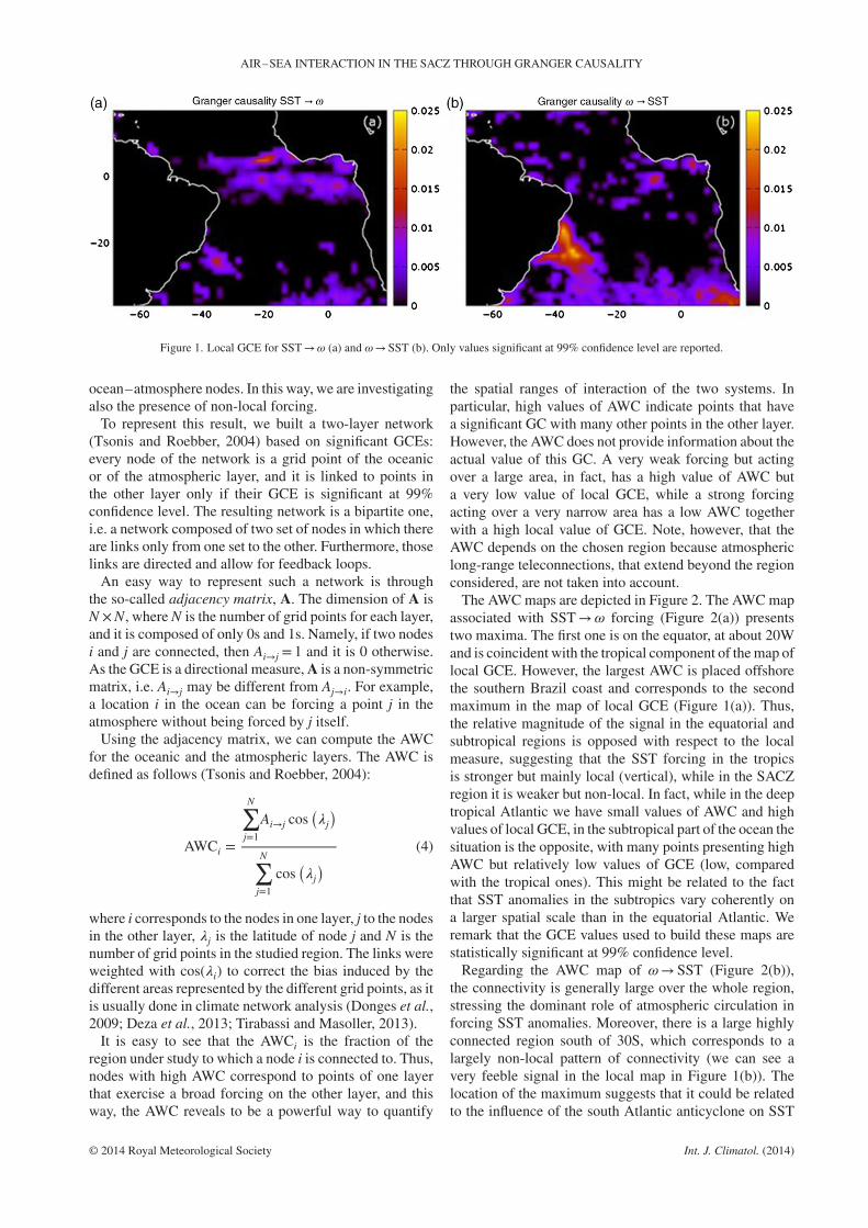
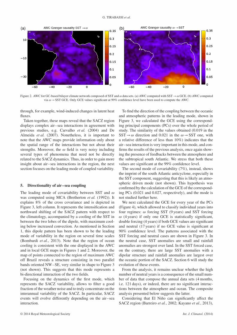
Figure 3. (Left column) Leading mode of coupled variability related to the 𝜔 and SST fields. Only significant values at 95% are reported. Thedashed line represents the climatological mean position of the SACZ. (Central column) Composites for convective maxima of oceanic forcing years(SST→𝜔 regime, see Section 5 for details). (Right column) Composites for convective maxima of years without significant air–ocean coupling

(neutral regime, see Section 5 for details). In the bottom left panel, the two boxes used for Figures 11 are depicted.

Figure 4. GCE between 𝜔 and SST PCs, relative to the leading modeof covariability. Non-significant (at 90%) GCE values are set to 0. (a)Example of years displaying of non-significant coupling, i.e. none of thetwo GCE values is significant. (b) Example of a year of oceanic forcing;only the SST to 𝜔 GCE value is significant. (c) Example of a year ofatmospheric forcing; just the 𝜔 to SST value is significant. (d) A year of

mutual forcing; both the values are significant.

we tried to relate the occurrences of the four differentregimes with the occurrence of El Niño as character-ized by the NINO3.4 index. Separating the whole periodin El Niño, La Niña and neutral years – according tothe Oceanic Niño Index (ONI) computed with NOAAERSSTv3b data – we can observe that the only signifi-cant combination (p< 0.1) is between neutral years andpure atmospheric forcing (see Table 1). In the table, thep-values are computed using a binomial distribution, tak-ing into account both the cardinality of ENSO and PC1classification sets. Thus, the analysis suggests that the cir-culation anomalies induced by El Niño and La Niña mod-ify the regional dynamics such that the number of events ofpure atmospheric forcing in the SACZ region decreases. Atthe same time, most of the years in which the SST forcingplays a role in the dynamics of the events (cases SST→𝜔

and SST↔𝜔) correspond to either El Niño or La Niñayears (six out of eight cases). This is discussed further inSection 6.

Table 1. Division of the various years composing the database,respecting to the GC and ENSO classification.

El Niño La Niña Neutral Total

Neutral 4 (p= 0.62) 8 (p= 0.19) 5 (p= 0.8) 17SST→𝜔 3 (p= 0.10) 0 1 4𝜔→ SST 2 1 6 (p= 0.08) 9SST↔𝜔 1 3 (p= 0.16) 0 4

Some p-values are reported. The p-values are computed using a binomialdistribution, taking into account both the cardinality of ENSO and PC1classification sets.

6. Evolution of events

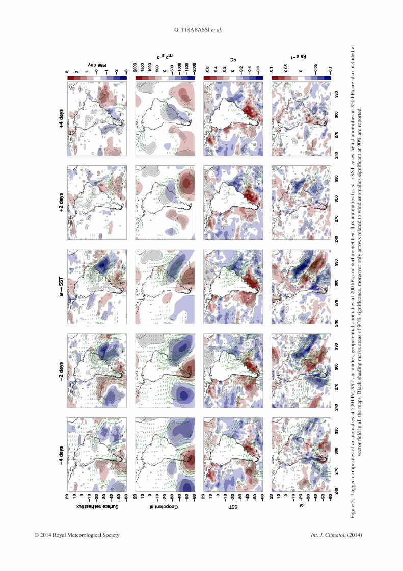
To study the evolution of the events in each of the four cate-gories defined before, we constructed composites using thePC of 𝜔 corresponding to the leading mode. Thus, by con-struction all cases present a dipole in the vertical velocityfield in the SACZ region, but the evolution of anomalieswill be different. To smooth out the fields, the MCA isperformed after a running-mean filtering over 3 days. Thecomposites are calculated as the difference between theaverage of the 5 days presenting the largest positive peaksin the 𝜔 PC, and the average of the 5 days presenting thelargest negative peaks taken from the subset of years cor-responding to each category. We then repeated this com-putation for [−4:4] days preceding and following the dayof the maximum value. The composites for the four cases(Figures 5–9) are constructed for 𝜔, SST, net surface heatfluxes, 850 hPa winds and geopotential height at 200 hPa.

6.1. Case 𝜔→ SST

Composites of the 𝜔 field (Figure 5, last row) clearly showthat the dipole starts developing at time −4 days and hasalmost disappeared at time +4 days (Figure 5, last row).In upper levels, the development of the dipole is accom-panied by a travelling wave train from the extratropicalPacific sector that bends into the SACZ region as thegeopotential composites show (Figure 5, second row). Thelower level wind anomalies are consistent with this wave

© 2014 Royal Meteorological Society Int. J. Climatol. (2014)

G. TIRABASSI et al.

Figu

re5.

Lag

ged

com

posi

tes

of𝜔

anom

alie

sat

500

hPa,

SST

anom

alie

s,ge

opot

entia

lano

mal

ies

at20

0hP

aan

dsu

rfac

ene

thea

tflux

anom

alie

sfo

r𝜔→

SST

case

s.W

ind

anom

alie

sat

850

hPa

are

also

incl

uded

asve

ctor

field

inal

lthe

map

s.B

lack

shad

ing

mar

ksar

eas

of90

%si

gnifi

canc

e,m

oreo

ver

only

arro

ws

rela

ted

tow

ind

anom

alie

ssi

gnifi

cant

at90

%ar

ere

port

ed.

© 2014 Royal Meteorological Society Int. J. Climatol. (2014)

AIR–SEA INTERACTION IN THE SACZ THROUGH GRANGER CAUSALITY

Figu

re6.

Lag

ged

com

posi

tes

of𝜔

anom

alie

sat

500

hPa,

SST

anom

alie

s,ge

opot

entia

lano

mal

ies

at20

0hP

aan

dsu

rfac

ene

thea

tflux

anom

alie

sfo

rneu

tral

case

.Win

dan

omal

ies

at85

0hP

aar

eal

soin

clud

edas

vect

orfie

ldin

allt

hem

aps.

Bla

cksh

adin

gm

arks

area

sof

90%

sign

ifica

nce,

mor

eove

ron

lyar

row

sre

late

dto

win

dan

omal

ies

sign

ifica

ntat

90%

are

repo

rted

.

© 2014 Royal Meteorological Society Int. J. Climatol. (2014)

G. TIRABASSI et al.

Figu

re7.

Lag

ged

com

posi

tes

of𝜔

anom

alie

sat

500

hPa,

SST

anom

alie

s,ge

opot

entia

lano

mal

ies

at20

0hP

aan

dsu

rfac

ene

thea

tflux

anom

alie

sfo

rSS

T→

𝜔ca

se.W

ind

anom

alie

sat

850

hPa

are

also

incl

uded

asve

ctor

field

inal

lthe

map

s.B

lack

shad

ing

mar

ksar

eas

of90

%si

gnifi

canc

e,m

oreo

ver

only

arro

ws

rela

ted

tow

ind

anom

alie

ssi

gnifi

cant

at90

%ar

ere

port

ed.

© 2014 Royal Meteorological Society Int. J. Climatol. (2014)

AIR–SEA INTERACTION IN THE SACZ THROUGH GRANGER CAUSALITY

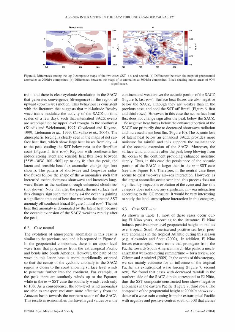
Figure 8. Differences among the lag-0 composite maps of the two cases SST→𝜔 and neutral. (a) Differences between the maps of geopotentialanomalies at 200 hPa composites. (b) Differences between the maps of 𝜔 anomalies at 500 hPa composites. Black shading marks areas of 90%

significance.

train, and there is clear cyclonic circulation in the SACZthat generates convergence (divergence) in the region ofupward (downward) motion. This behaviour is consistentwith the literature that suggests that mid-latitude Rossbywave trains modulate the activity of the SACZ on timescales of a few days, such that intensified SACZ eventsare accompanied by upper level troughs to the southwest(Kiladis and Weickmann, 1997; Cavalcanti and Kayano,1999; Liebmann et al., 1999; Carvalho et al., 2004). Theatmospheric forcing is clearly seen in the maps of net sur-face heat flux, which show large heat losses from day −4to the peak cooling the SST below next to the Braziliancoast (Figure 5, first row). Regions with southeasterliesinduce strong latent and sensible heat flux loses between[55W–30W, 30S–50S] up to day 0; after the peak, thelatent and sensible heat flux anomalies change sign (notshown). The pattern of shortwave and longwave radia-tive fluxes follow the shape of the 𝜔 anomalies such thatincreased ascent decreases shortwave and increases long-wave fluxes at the surface through enhanced cloudiness(not shown). Note that after the peak, the net surface heatflux changes sign such that at day +4 the ocean is gaininga significant amount of heat that weakens the created SSTanomaly off southeast Brazil (Figure 5, third row). The netheat flux anomaly is dominated by the latent heat becausethe oceanic extension of the SACZ weakens rapidly afterthe peak.

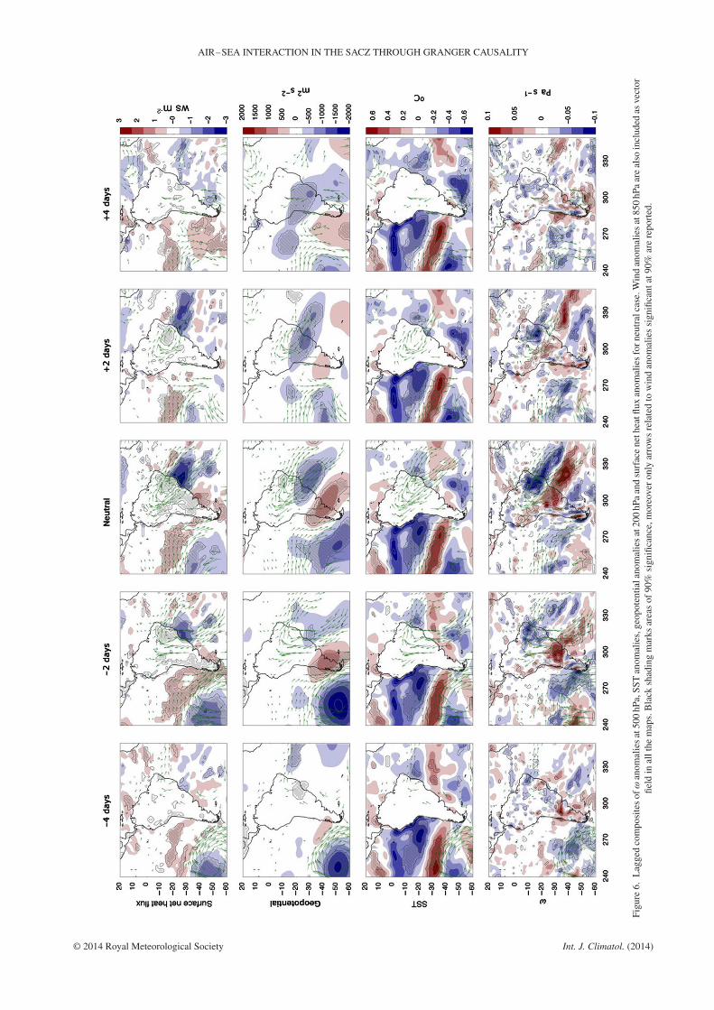
6.2. Case neutral

The evolution of atmospheric anomalies in this case issimilar to the previous one, and it is reported in Figure 6.In the geopotential composites, there is an upper levelwave train that progresses from the extratropical Pacificand bends into South America. However, the path of thewave in this latter case is more meridionally orientedso that the centre of the cyclonic anomaly in the SACZregion is closer to the coast allowing surface level windsto penetrate further into the continent. For example, atthe peak there are southerly winds up to the Equator,while in the 𝜔→ SST case the southerly winds reach onlyto 10S. As a consequence, the low-level wind anomaliesare able to transport moisture more effectively from theAmazon basin towards the northern sector of the SACZ.This results in𝜔 anomalies that have largest values over the

continent and weaker over the oceanic portion of the SACZ(Figure 6, last row). Surface heat fluxes are also negativebelow the SACZ, although they are weaker than in theprevious case, and cool the SST off Brazil (Figure 6, firstand third rows). However, in this case the net surface heatflux does not change sign after the peak below the SACZ.The negative heat fluxes below the enhanced portion of theSACZ are primarily due to decreased shortwave radiationand increased latent heat flux (Figure 10). The oceanic lossof latent heat below an enhanced SACZ provides moremoisture for rainfall and thus supports the maintenanceof the oceanic extension of the SACZ. Moreover, thesurface wind anomalies after the peak keep blowing fromthe ocean to the continent providing enhanced moisturesupply. Thus, in this case the persistence of the oceanicportion of the SACZ is larger than in the 𝜔→ SST case(see also Figure 10). Therefore, in the neutral case thereseems to exist two-way air–sea interaction. However, asthe largest anomalies occur over land, this process does notsignificantly impact the evolution of the event and thus thiscategory does not show any significant air–sea interactionaccording to the GC measure. It would be very interestingto study the land–atmosphere interaction in this category.

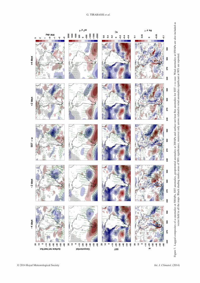
6.3. Case SST→𝜔

As shown in Table 1, most of these cases occur dur-ing El Niño years. According to the literature, El Niñoinduces positive upper level geopotential height anomaliesover tropical South America and positive sea level pres-sure anomalies in the tropical Atlantic during this season(e.g. Alexander and Scott (2002)). In addition, El Niñoforces extratropical wave trains that propagate from thePacific towards South America in arch-like paths, a mech-anism that weakens during summertime – for a review, seeGrimm and Ambrizzi (2009). In the events of this category,we see mainly evidence for an influence of the tropicalPacific via extratropical wave forcing (Figure 7, secondrow). We found that cases with decreased rainfall in thenorthern side of the SACZ dipole correspond to El Niño,thus the SST composite constructed here shows negativeanomalies in the eastern Pacific (Figure 7, third row). Thecomposite of the geopotential height at 200 hPa shows evi-dence of a wave train coming from the extratropical Pacificwith negative and positive centres south of 50S that arches

© 2014 Royal Meteorological Society Int. J. Climatol. (2014)

G. TIRABASSI et al.

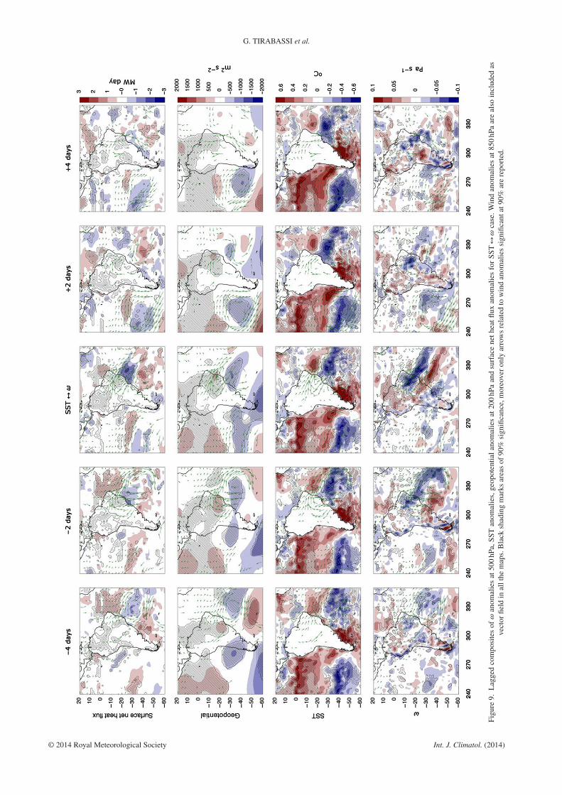
Figu

re9.

Lag

ged

com

posi

tes

of𝜔

anom

alie

sat

500

hPa,

SST

anom

alie

s,ge

opot

entia

lano

mal

ies

at20

0hP

aan

dsu

rfac

ene

thea

tflux

anom

alie

sfo

rSS

T↔

𝜔ca

se.W

ind

anom

alie

sat

850

hPa

are

also

incl

uded

asve

ctor

field

inal

lthe

map

s.B

lack

shad

ing

mar

ksar

eas

of90

%si

gnifi

canc

e,m

oreo

ver

only

arro

ws

rela

ted

tow

ind

anom

alie

ssi

gnifi

cant

at90

%ar

ere

port

ed.

© 2014 Royal Meteorological Society Int. J. Climatol. (2014)

AIR–SEA INTERACTION IN THE SACZ THROUGH GRANGER CAUSALITY

Figu

re10

.C

ompo

site

sof

surf

ace

heat

com

pone

nts

and

win

dan

omal

ies

at85

0hP

afo

rth

ene

utra

lcas

e.B

lack

shad

ing

mar

ksar

eas

of90

%si

gnifi

canc

e,on

lyar

row

sre

late

dto

win

dan

omal

ies

sign

ifica

ntat

90%

are

repo

rted

.

© 2014 Royal Meteorological Society Int. J. Climatol. (2014)

G. TIRABASSI et al.

towards the tropical Atlantic to the east of South America.This wave train has a stationary component as the cen-tres of the anomalies move slowly from day −4 to day+4 (Figure 7, second row). In addition to the wave train,there is a positive geopotential height anomaly centred at(40S, 90W) that persist during the whole event. This is inclear contrast to the previous two cases (e.g. 𝜔→ SST andneutral, Figures 5 and 6) and indicates the influence of thetropical Pacific forcing. Superposed on the stationary wavecomponent, there is a travelling wave train that shifts thepattern westward and intensifies the atmospheric anoma-lies. The resulting path of the wave is quite south and thesurface wind anomalies in the SACZ region are locatedmainly over the ocean. Thus, the 𝜔 anomalies in Figure 7are strongest in the oceanic portion of the SACZ with onlyweak continental extension. Moreover, the oceanic dipoleof 𝜔 anomalies persists up to day +4, albeit weakeningwith time.

To further illustrate the distinct behaviour of this casewith respect to the previous one, in Figure 8 we report thedifference in atmospheric circulation anomalies betweenSST→𝜔 and neutral cases at the peak of the event. Consis-tent with the previous description, the geopotential differ-ence shows a ridge over the continent and a trough over theocean indicating that the negative geopotential anomaliesin the SST→𝜔 are shifted over the ocean. Furthermore,due to its barotropic structure the ridge over eastern Brazilis associated with increased northerlies into the subtrop-ics and easterlies in northeast Brazil. This induces mois-ture flux anomalies and the continental convection dipoleobserved in Figure 8(b), which indicates smaller conti-nental rainfall anomalies in the SST→𝜔 compared withthe neutral case. In higher latitudes, there are large differ-ences in the geopotential field reflecting differences in thebehaviour of the wave associated with the two cases andmentioned before.

On the oceanic side, the Atlantic SST anomaly field isdominated by a strong dipole with cold anomalies northof 30S and warm anomalies to the south, except to thesouth of Uruguay. This SST pattern is conspicuous duringsummertime and is related to a strengthening of the southAtlantic anticyclone on seasonal time scales (Barreiroet al., 2004). As in the previous cases, there is strong heatloss off Brazil from day −4 to the peak, which cools theSST below. The southeasterly component of the surfacewinds provide more moisture to the region of enhancedascent. Moreover, in the days following the peak, thereis oceanic latent heat loss below the region of anomalousascent which, as in the Neutral case, implies anomalousmoisture flux into the atmosphere that helps maintainingthe 𝜔 (rainfall) anomalies over the oceanic portion of theSACZ up to day +4 (Figures 6 and 7). In this case, asmost of the atmospheric anomalies are located over theocean, the evolution of the rainfall dipole is influenced bythe SST. These results suggest that of central importancefor the SST to influence the evolution of SACZ events isthat atmospheric anomalies have to be located mainly overthe ocean. According to our results, this means that theextratropical wave trains have to propagate mainly zonally

and bend only slightly into the tropical Atlantic. Since3 out of 4 years in this category correspond to El Niñoyears, it suggests that changes in the mean state causedby a warming in the equatorial Pacific may change thepropagation properties of the wave trains through changesin the jet streams or blocking as found during winter byOliveira et al. (2014). More research is needed to fullyaddress this issue , including understanding what is specialabout these three El Niño events.

6.4. Case SST↔𝜔

According to Table 1, most of these cases occur during LaNiña years and correspond to years with dipole events thathave negative rainfall anomalies in the northern portion ofthe SACZ (Figure 9). Contrary to the case SST→𝜔, herethe tropical anomalies induced by the equatorial PacificOcean are more significant than the extratropical waveforcing (compare composites for the geopotential height in200 hPa and for the surface winds in Figures 7 and 9). Asconsequence, there are northwesterly surface wind anoma-lies in northeastern Brazil that last the whole event andhelp the development of convergence there (Figure 9, sec-ond row). In addition, over the continental SACZ region,there is a positive geopotential height anomaly that, due toits baroclinic nature, has a low pressure associated at thesurface that seems to play an important role in the event.Together with the low-pressure centre associated with aweak extratropical wave train, they generate the cyclonicwind anomaly associated with the peak rainfall dipole inthe SACZ. Note that at day −4 the convective anomaliesover land and over the ocean develop separately and mergeat day −2 when the surface low-pressure centre over theocean moves westward. The travelling wave train in thegeopotential composites is the weakest of all four cate-gories having the maximum at day −4. At the peak, thesurface wind anomalies and oceanic heat loss are relativelyweak (Figure 9, first row). At day +2, there is a dipolein surface net heat flux anomalies with similar structurebut weaker in magnitude than the one in SST→𝜔 case,but at day +4 heat fluxes are no longer significant. Finally,the region of ascent motion over the continent lasts fromday −4 to day +4, the longest of all categories, probablydue to the favourable conditions maintained by El Niño(Figure 9, last row). As anomalies are relatively weak andEl Niño seems to play an important role, it is hard to pin-point how the ocean and atmosphere interact and morework is needed to understand this case. One possibilitywould be to repeat the Granger analysis after removing ElNiño influence, but that is beyond the scope of this study.

As an additional analysis to compare the four regimes,we report in Figure 11 the time evolution of 𝜔 anomalyin the composites computed in two different boxes: one inthe continental box [22S; 6S]× [55W; 35W], and anotherin an oceanic box at [40S; 30S]× [40W; 1W]. The twoboxes, depicted in Figure 3, were chosen to characterizethe strength of the anomalies over the continent and theoceanic extension of the SACZ. The lag times in Figure 11

© 2014 Royal Meteorological Society Int. J. Climatol. (2014)

AIR–SEA INTERACTION IN THE SACZ THROUGH GRANGER CAUSALITY

Figure 11. Composites of average 𝜔 anomalies in Continental ([22S;6S]× [55W;35W] (a) and Oceanic ([40S;30S]× [40W,1W] (b) boxes (see textfor details).

are the same of Figures 5–7 and 9, thus the 0 lag corre-sponds to the convective peak. It can be seen that the over-all evolution of anomalies over the continental region arequite symmetric about day 0, except in the case of oceanforcing. In this latter case, the peak occurs at day +1 andanomalies tend to persist. Over the oceanic region, anoma-lies are generally smaller in magnitude and have similarvalues at day −1 and day 0. The neutral case is the onecharacterized by weakest positive precipitation anomaliesover the ocean and largest over the continent. The SST→𝜔

case, on the other hand, shows weakest rainfall anomaliesover the continent, but has largest persistence of anoma-lies over the ocean. Cases 𝜔→ SST and SST↔ show avery similar evolution over the continent, except at the endof the event when cases SST↔𝜔 have larger persistence.Over the ocean, case 𝜔→ SST shows the largest anoma-lies, but do not persist for long: after the peak, the verticalvelocity rapidly goes back to zero at day +2. This is insharp contrast with the case SST→𝜔 where anomalies atday +2 are still large.

7. Summary

Air–sea interactions in the region of the SACZ are studiedusing the GCE as a measure of directional coupling. Afirst important result is that this region has a large mutualair–sea connectivity during summertime. Introducing anew method that combines GC with MCA, we have beenable to identify four regimes, depending on the directionof the air–sea interaction. In particular, we identified yearsin which the coupling is mainly directed from the ocean tothe atmosphere, years in which the coupling is from theatmosphere to the ocean, years of mutual interactions andyears of no significant coupling.

We studied the evolution of the convective eventsrelated to these different regimes looking at atmosphericand surface oceanic fields and found that in all cases anextratropical wave train plays a major role in forcingconvection in the SACZ, as suggested previously byseveral authors. Moreover, we found that the path ofthe wave seems to be instrumental in determining theevolution of the SACZ event. For example, if the path

of the wave bends significantly over South America, thelargest anomalies develop first and are more intense overthe continent, the oceanic extension of the SACZ is weakand there is no air–sea coupling (Neutral cases). On theother hand, in ocean-forced cases, the extratropical wavetrain is further to the south so that the strongest convectiveanomalies develop over the oceanic portion of the SACZ,allowing the ocean to force atmospheric anomalies thattend to persist longer than in other regimes. We also foundthat these events are more frequent during El Niño years.

Further study of the SACZ using this methodologycombined with tailored numerical experiments that, forexample, isolate the effects of El Niño are needed to furtherunderstand the complex air–sea interactions in this region.

Acknowledgements

This work was supported by the LINC project(FP7-PEOPLE-2011-ITN, Grant No. 289447). C. M.acknowledges partial support from grant FIS2012-37655-C02-01 from the Spanish MCI, and the ICREA Academiaprogramme.

References

Alexander M, Scott J. 2002. The influence of ENSO on air-sea interac-tion in the Atlantic. Geophys. Res. Lett. 29(14): 46–49.

Attanasio A, Pasini A, Triacca U. 2012. A contribution to attribution ofrecent global warming by out-of-sample Granger causality analysis.Atmos. Sci. Lett. 13(1): 67–72.

Barreiro M, Chang P, Saravanan R. 2002. Variability of the SouthAtlantic Convergence Zone as simulated by an atmospheric generalcirculation model. J. Clim. 15: 745.

Barreiro M, Giannini A, Chang P, Saravanan R. 2004. On the role of theSouth Atlantic atmospheric circulation in tropical Atlantic variability.In Earth’s Climate, Wang C, Xie SP, Carton JA (eds). AmericanGeophysical Union: Washington, DC, doi: 10.1029/147GM08.

Barreiro M, Chang P, Saravanan R. 2005. Simulated precipitationresponse to SST forcing and potential predictability in the region ofthe South Atlantic Convergence Zone. Clim. Dyn. 24: 105–114.

Bombardi RJ, Carvalho LMV, Jones C, Reibota MS. 2013. Precipitationover eastern South America and the South Atlantic sea surface tem-perature during Neutral ENSO periods. Clim. Dyn. 42: 1553–1568.

Bretherton CS, Smith C, Wallace JM. 1992. An intercomparison ofmethods for finding coupled patterns in climate data. J. Clim. 5:541–560.

© 2014 Royal Meteorological Society Int. J. Climatol. (2014)

G. TIRABASSI et al.

Carvalho LMV, Jones C, Liebmann B. 2002. Extreme precipitationevents in southeastern South America and large-scale convectivepatterns in the South Atlantic Convergence Zone. J. Clim. 15:2377–2394.

Carvalho LMV, Jones C, Liebmann B. 2004. The South Atlantic Con-vergence Zone: intensity, form, persistence, and relationships withintraseasonal to interannual activity and extreme rainfall. J. Clim. 17:88–107.

Cavalcanti IFA, Kayano MT. 1999. High-frequency patterns of theatmospheric circulation over the Southern Hemisphere and SouthAmerica. Meteorol. Atmos. Phys. 69(3–4): 179–193.

Chatfield C. 1989. The Analysis of Time Series: An Introduction, 4th edn.Chapman & Hall: New York, NY.

Chaves RR, Nobre P. 2004. Interactions between sea surface temperatureover the South Atlantic Ocean and the South Atlantic ConvergenceZone. Geophys. Res. Lett. 31: L03204, doi: 10.1029/2003GL018647.

De Almeida RAF, Nobre P, Haarsma RJ, Campos EJD. 2007. Negativeocean-atmosphere feedback in the South Atlantic Convergence Zone.Geophys. Res. Lett. 34(18): L18809.

Dee DP, Uppala SM, Simmons AJ, Berrisford P, Poli P, Kobayashi S,Andrae U, Balmaseda MA, Balsamo G, Bauer P, Bechtold P, BeljaarsACM, van de Berg L, Bidlot J, Bormann N, Delsol C, Dragani R,Fuentes M, Geer AJ, Haimberger L, Healy SB, Hersbach H, HólmEV, Isaksen L, Kållberg P, Köhler M, Matricardi M, McNally AP,Monge-Sanz BM, Morcrette J-J, Park B-K, Peubey C, de Rosnay P,Tavolato C, Thépaut J-N, Vitart F. 2011. The ERA-Interim reanalysis:configuration and performance of the data assimilation system. Q. J.R. Meteorol. Soc. 137: 553–597.

Deza JI, Barreiro M, Masoller C. 2013. Inferring interdependencies inclimate networks constructed at inter-annual, intra-season and longertime scales. Eur. Phys. J. Spec. Top. 222(2): 511–523.

Donges JF, Zou Y, Marwan N, Kurths J. 2009. The backbone of theclimate network. EPL 87: 4.

Grimm AM, Ambrizzi T. 2009. Teleconnections into South Americafrom the tropics and extratropics on interannual and intraseasonaltimescales. In Past Climate Variability in South America and Sur-rounding Regions. Springer: London, 159–191.

Hoskins BJ, Karoly DJ. 1981. The steady linear response of a sphericalatmosphere to thermal and orographic forcing. J. Atmos. Sci. 38:61179–61196.

Junquas C, Vera C, Li L, Le Treut H. 2012. Summer precipitationvariability over Southeastern South America in a global warmingscenario. Clim. Dyn. 38(9–10): 1867–1883.

Kayano MT, Andreoli RV, Ferreira de Souza RA. 2013. Relationsbetween ENSO and the South Atlantic SST modes and their effectson the South American rainfall. Int. J. Climatol. 33: 2008–2023, doi:10.1002/joc.3569.

Khokhlov VN, Glushkov AV, Loboda NS. 2006. On the nonlinearinteraction between global teleconnection patterns. Q. J. R. Meteorol.Soc. 132(615): 447–465.

Kiladis GN, Weickmann KM. 1997. Horizontal structure and season-ality of large-scale circulations associated with submonthly tropicalconvection. Mon. Weather Rev. 125(9): 1997–2013.

Kodama YM. 1992. Large-scale common features of subtropical precip-itation zones (the Baiu frontal zone, the SPCZ, and the SACZ). Part I:characteristics of subtropical frontal zones. J. Meteorol. Soc. Jpn. 70:813–836.

Liebmann B, Kiladis GN, Marengo JA, Ambrizzi T, Glick JD. 1999.Submonthly convective variability over South America and the SouthAtlantic Convergence Zone. J. Clim. 12(7): 1877–1891.

Mokhov II, Smirnov DA, Nakonechny PI, Kozlenko SS, Seleznev EP,Kurths J. 2011. Alternating mutual influence of El-Niño/SouthernOscillation and Indian monsoon. Geophys. Res. Lett. 38: L00F04.

Mosedale TJ, Stephenson DB, Collins M, Mills TC. 2006. Grangercausality of coupled climate processes: ocean feedback on the NorthAtlantic Oscillation. J. Clim. 19: 1182.

Nogués-Paegle J, Mo KC. 1997. Alternating wet and dry conditions overSouth America during summer. Mon. Weather Rev. 125: 2.

Oliveira FNM, Carvalho L, Ambrizzi T. 2014. A new climatology forSouthern Hemisphere blockings in the winter and the combined effectof ENSO and SAM phases. Int. J. Climatol. 34(5): 1676–1692.

Pasini A, Triacca U, Attanasio A. 2012. Evidence of recent causaldecoupling between solar radiation and global temperature. Environ.Res. Lett. 7: 3.

Robertson AW, Mechoso CR. 2000. Interannual and interdecadal vari-ability of the South Atlantic Convergence Zone. Mon. Weather Rev.128(8): 2947–2957.

Runge J, Petoukhov V, Kurths J. 2014. Quantifying the strength anddelay of climatic interactions: the ambiguities of cross correlation anda novel measure based on graphical models. J. Clim. 27(2): 720–739.

Salvucci GD, Saleem JA, Kaufmann R. 2002. Investigating soil moisturefeedbacks on precipitation with tests of Granger causality. Adv. WaterResour. 25(8): 1305–1312.

Schwarz G. 1978. Estimating the dimension of a model. Ann. Stat. 6(2):461–464.

Stern DI, Kaufmann RK. 1999. Econometric analysis of global climatechange. Environ. Model. Softw. 14(6): 597–605.

Stern DI, Kaufmann RK. 2014. Anthropogenic and natural cause ofclimate change. Clim. Change 122(1–2): 247–269.

Tirabassi G, Masoller C. 2013. On the effects of lag-times in networksconstructed from similarities of monthly fluctuations of climate fields.EPL 102: 5.

Tsonis AA, Roebber PJ. 2004. The architecture of the climate network.Phys. A 333: 497–504.

© 2014 Royal Meteorological Society Int. J. Climatol. (2014)