a study of simulated annealing and a revised cascade algorithm for image reconstruction
TRANSCRIPT

Statist ics and Comput ing 5, (1995) 175-190
A study of simulated anneal&g and a rev&ed cascade algorithm for image reconstruction
M E R R I L E E H U R N and C H R I S T O P H E R J E N N I S O N
School of Mathematical Sciences, University of Bath, Bath, BA2 7A Y, UK
Received June 1993 and accepted October 1994
We describe an image reconstruction problem and the computational difficulties arising in determining the maximum a posteriori (MAP) estimate. Two algorithms for tackling the problem, iterated conditional modes (ICM) and simulated annealing, are usually applied pixel by pixel. The performance of this strategy can be poor, particularly for heavily degraded images, and as a potential improvement Jubb and Jennison (1991) suggest the cascade algorithm in which ICM is initially applied to coarser images formed by blocking squares of pixels. In this paper we attempt to resolve certain criticisms of cascade and present a version of the algorithm extended in definition and implementation. As an illustration we apply our new method to a synthetic aperture radar (SAR) image. We also carry out a study of simulated annealing, with and without cascade, applied to a more tractable minimization problem from which we gain insight into the properties of cascade algorithms.
Keywords: Image analysis, MAP estimation, optimization, simulated annealing, multi-resolution
1. The image reconstruction problem
Directly observed images are a source of information in many application areas: satellites measure reflectance from the Earth's surface to provide maps of land use, and the X-ray energy detected through a body is presented as a medical image. These recorded images may be for visual use, a doctor's diagnosis of a broken bone, or for further numerical processing, perhaps calculating the prevalence of a particular crop. It is often the case that the recorded data do not accurately represent the underlying scene. Degradation can occur in a number of ways, for example, blurring as a result of atmospheric motion, or thermal noise in the detector (for more details see Geman, 1990). The image reconstruction problem is to estimate the true scene given the observed data.
We will assume that the image is digitized, and that we record a real-valued vector Y = (Y1, Y2,.-., Ys) T where Ys, s = 1 , . . . , S, is the observation for the sth pixel. The unobservable scene X is also taken to be digitized and, in addition, discretized so that at any pixel s, Xs can take an integer value in the set (0, 1 , . . . , N - 1 } . Geman and Geman (1984) propose a commonly used model for Y, incorporating degradation by shift-invariant blurring which can be represented by a matrix K acting on X, which is generally larger than Y, plus additive pixel-wise 0960-3174 �9 1995 Chapman & Hall
independent normal noise,
Y = K X + rl (1)
where 7/s "~ N(0, cr2). Geman and Geman then advocate a Bayesian approach,
using equation (1) to formulate a likelihood for the data given the scene, P ( Y = y I X = x), and specify a locally dependent Markov random field model as a scene prior, P ( X = x). This class of models is defined by the fact that the conditional probability of a pixel s taking a certain value, given the value of X at the remaining pixels, depends only on the X values at a small number of nearby pixels, known as the neighbours of s. Denoting the neighbours of s by 6s, and all components of X other than the sth by X_s, this definition may be expressed as P(Xs = xs [X_s = x_s) = P(Xs = xs IX, = xt,Vt E 6s). The conditional independence of pixels which are not neighbours of one another provides an enormous computa- tional saving in updating pixels in simulation algorithms such as the Gibbs sampler, or optimization methods such as simulated annealing and ICM. A set of pixels, all of which are neighbours of each other in a Markov random field model, is called a clique; we shall denote a single clique by c and the set of all cliques by C. In determining the forms these models take, the Hammersley-Clifford theorem states that, under a positivity condition, a distribution P ( X = x)

176 Hurn and Jennison
is a Markov random field if, and only if, it can be written in the form
P(X = x) = e x p ( - ~ ( x ) ) / Z (2)
where ~(x) = )--]~c~C ~c(x), the sum over cliques of func- tions involving only pixels in each clique. The Markov random field models express the prior belief that the image is smooth, where this is usually taken to mean locally constant (but see Geman and Reynolds, 1992, for exten- sions to locally planar or quadratic surfaces). The function ~r penalises roughness in the x values of pixels in the clique c. We can now express the posterior distribution of the image given the data, at least up to proportionality:
P(X = x I Y =Y)cx exp( -cb(x) - Ily- Kxll2/(2tr2)) (3)
In this paper we study the problem of finding the maximum a posteriori (MAP) reconstruction, that is the image which maximizes the posterior probability indicated by equation (3). An equivalent estimate is the x which minimizes the function H(x) = r + Ily- gxl12/(2a2), which Geman and Geman (1984) refer to as the 'energy'. Other estimates are possible, for example the marginal posterior mode at each pixel. We shall not reiterate argu- ments concerning the relative merits of MAP and other estimates but refer the interested reader to, for example, Besag (1986), Marroquin et al. (1987), Ripley (1988), Grieg et al. (1989), and in particular the recent work of Rue (1994). Our methods for finding closer approximations to the MAP estimate are obviously of use to those who choose to use this method; use of more accurate MAP estimates is also desirable in studies designed to compare different estimates.
In Section 2, we describe the standard approaches to finding the MAP estimate, before describing a modi- fication of an existing cascade algorithm in Section 3. In Section 4, we present an assessment of cascade and simulated annealing in minimizing two test functions which permit exact monitoring. We return to the image problem in Section 5.
2. Single-site algorithms for MAP estimation
2.1. Simulated annealing
It is not a simple task to identify the MAP estimate by minimizing the energy function H(x). When each of the S pixels can take one of N values {0, 1 , . . . , N - 1}, there
S are N possible scenes x. Denote the space of these possible images by f~. Even for small two-colour scenes, it is compu- tationally infeasible to attempt the minimization by an exhaustive search of f~. Geman and Geman (1984) suggest applying the stochastic relaxation algorithm, simulated annealing; this algorithm was earlier considered by Kirk- patrick et al. (1983), although not in the imaging context.
In outline, simulated annealing draws a sequence of samples from the temperature Tk distributions,
pk(X ) = exp( -H(x) /Tk) x E f~ (4) Zk
as the non-increasing temperature schedule {Tk;k = 1,2,. . . } tends to zero. The distribution pk(x) is the posterior distribution of equation (3) raised to the power 1/Tk and suitably renormalized. Thus, as T k -~ 0, this powered-up distribution increasingly concentrates on those x which have high posterior probability.
Complexity prevents direct sampling from any particular pk(x); Hastings (1970) suggests an indirect approach. The general Hastings algorithm is iterative: given some state x (t) E f~ at step t, a potential new state x' is generated from the proposal distribution q(x (t), x'). With probability a(x (t), x'), x' is accepted as the next state x (t+ 1), otherwise x (t) is retained. The algorithm then has Markov chain transition function
q(x, x')c~(x, x') x' # x e(x, x') = 1 - E e(x, x") x' = x (5)
X tt ~ X
Considering for the moment a single fixed temperature distribution pk(x), the distribution of the sequence X (~ X(I),... converges to the distribution p~(x) as t ~ c~, pro- vided P(x, x r) is irreducible, aperiodic, and satisfies detailed balance with respect to pk(x),
P(x,x')pk(x) = P(x',x)pk(x'), VX, X' E ~2 (6)
Peskun (1973) shows that the optimal choice of a(x, x'), to ensure detailed balance and minimize the asymptotic variance of ergodic averages calculated from the sequence, is
a(x, x') = min{ 1 q(x', x)pk(x') "' q(x, x')pk(X) } (7)
The different choices for q(x, x') then distinguish between the specific examples of Hastings algorithms.
One prerequisite for the proposal distribution is that it be easier to sample than the original pk(x). For this reason, an extremely common restriction is that q(x, x') is zero unless x and x' differ at most at just one pixel. Algorithms satisfying this constraint are known as sing&- site update methods; the well-known Metropolis algorithm (Metropolis et al., 1953) and Gibbs sampler are both included in this category. A pixel s is chosen to be updated, either randomly or as part of a systematic sweep
/ of the image. In the Metropolis algorithm, a new value x s is chosen uniformly after excluding the current value, x s. The resulting qM(X,X') is symmetric in x and x t, and equation (7) simplifies to
O~M(X,X t) : min( 1, pk(x') p (x) J (8)

Simulated annealing and a revised cascade algorithm for image reconstruction 177
The Gibbs sampler was described by Geman and Geman (1984). When pixel s is updated, the permitted images x I are proposed proportional to their probabilities under
~ , if ' X _ s = X _ s
qa(x,x') = pk(X") (9) X rt : X l t s ~ X s
0, otherwise
Using equation (7) the acceptance probability correspond- ing to qG(x, x') is identically 1, that is the Gibbs sampler has zero rejection.
Hastings algorithms require a certain number of iterations to 'burn in', or reach the equilibrium distribu- tion from an arbitrary starting configuration. With simulated annealing, we have only one iteration in which to attempt to draw a sample from the kth temperature distribution using the ( k - 1)th realization as a starting point. This imposes restrictions upon the temperature schedules {Tk} which can be used if we wish to guarantee convergence to the MAP estimate. Geman and Geman (1984) consider simulated annealing based on the Gibbs sampler; they show that T k _> c*/log(1 + k) is a sufficient condition for convergence in probability, where c* is a large constant determined by the energy function. Hajek (1988) finds a necessary and sufficient condition for convergence of Metropolis-based annealing, namely ~ = l e x p ( - d * / T k ) = +cx~, where again d* is a constant depending upon H(x); this condition is satisfied by a schedule of the form Tk = c/log(1 + k) provided c _> d*.
2.2. Iterated conditional modes
As a far quicker alternative to simulated annealing, Besag (1986) proposes the deterministic ICM algorithm which ensures convergence at least to a local minimum of the energy function. At each pixel s in turn, the new value Xs is chosen to minimize the energy function H(x) holding all other pixel values x_s fixed. The ICM procedure is a strictly downhill search algorithm; unlike simulated anneal- ing, it cannot escape from local minima and is extremely sensitive to the starting configuration. A major objective of some of the cascade methods presented in this paper is to match the performance of simulated annealing with speed comparable to ICM.
3. The cascade algorithm
3.1. Multiple-site updating
Local minima are in some sense created by the scheme of pixel updating: if all pixels are updated simultaneously then we could move to the global minimum in a single step. A more realistic goal is to update a small number of
pixels together, but even then complications arise. In updat- ing n > 1 pixels at a time under simulated annealing, we need to sample the Hastings proposal efficiently when q(x, x') is now n-dimensional. Equivalently with ICM, the minimization must take place over a set of size N n.
Despite the extra computational burden, multiple-site updating is worth considering. Amit and Grenander (1991) demonstrate that the convergence rate of a fixed- temperature Hastings algorithm for a particular class of models may be improved by updating more than one site at a time. Indeed, in situations where 'critical slowing down', i.e. excessive correlation between successive samples, is a problem, multiple-site updating may be the only way to avoid becoming trapped almost indefinitely in one mode of the target distribution. Critical slowing down is inescapable in the low-temperature stages of simulated annealing. Existing sampling approaches which include multiple updates while remaining computationally feasible are the algorithm of Swendsen and Wang (1987) and its modifications by Edwards and Sokal (1988) and Hurn (1994), Metropolis-coupled Monte Carlo Markov chains (Geyer, 1991), and the multigrid approach (Sokal, 1989).
The algorithms mentioned above tackle sampling prob- lems relevant to simulated annealing but not to ICM. However, ICM is badly affected by local minima and multiple-site updates will allow escape from at least some of these. The renormalization group approach (Gidas, 1989) and the cascade algorithm (Jubb and Jennison, 1991) both attempt to generate a sequence of progressively smaller minimization problems akin to processing on var- ious scales. These nested multiple problems are intended to simplify the original H(x) minimization; they are tackled in order, using either standard single-site ICM or simulated annealing at each stage.
3.2. The Jubb-Jennison cascade
Jubb and Jennison (1991) present the cascade algorithm as a simple and efficient means of adapting ICM to cope with very noisy data. They are motivated by the task of restoring an unblurred image with low signal-to-noise ratio. In effect, to increase the signal-to-noise ratio, they average records within non-overlapping 2 • 2 blocks of pixels; they regard the result as the record for an image consisting of fewer, 'big' pixels, now with the noise variance quartered, a2/4. The blocking and averaging is repeated, producing a hierarchy of successively coarser resolution images.
In Jubb and Jennison's binary example, the energy function is of the form
S
H(x) = Z/3Iix,#x,] + (2or 2) 1 Z ( y s - xs) 2 (10) ( s , t ) s = 1
where (s, t) denotes a neighbouring pair of pixels s and t and I[x,#x,] is an indicator function taking the value 1 when

178 Hurn and Jennison
x~ ~ xt and 0 otherwise. At the mth coarsened resolution, where we will denote the averaged records by y(m) and the 'big' pixel values by X (m), Jubb and Jennison choose to define the energy function by using the same functional form for the prior distribution of X (m), namely
n(m)(x(m))=E~I[x!m)~x,m)]--~-(2~) -1 (S,t) • E ( y ! m) - x!m)) 2 (11)
where (s, t) now indicates an unordered pair of adjacent 'big' pixels on the ruth level pixel grid, L (m) say, and the second sum is, similarly, over these 'big' pixels. Processing of the cascade of images proceeds in a coarse-to-fine direction, passing down the ICM reconstruction from the appropriate energy function at one level as the starting configuration for ICM on the level below.
3.3. A modification of the algorithm
Cascade is appealing as a means of providing a good start- ing configuration for the original resolution problem since it is computationally cheap and, in the examples of Jubb and Jennison (1991), it appears quite effective. However, there are two objections to the algorithm as it stands. First, it is not apparent how to extend the aggregation ideas to blurred records, where averaging will alter the structure of the blurring. Second, and perhaps more importantly, it is not clear how the energy functions at different cascade levels are connected.
Our suggestion is that the 'big' pixels be regarded as blocks of the original resolution pixels constrained to take a common value. For the moment these blocks con- tinue to be 2 m • 2 m in size, although we will discuss more flexible schemes in Section 5. The energy of any con- figuration at any blocking level is then defined to be the energy calculated on the original resolution using the origi- nal unaveraged records. Although Jubb and Jennison only used ICM at each cascade level, one may just as easily apply simulated annealing as long as the initial temperature at each level is not so high that the advantages of a well- chosen starting image are lost. Algorithms are applied at the higher cascade levels by updating the x value of a big pixel, or equivalently the common x value of all the original pixels contained therein.
As a result of our proposed changes, there is no difficulty in extending cascade to deal with blurred images. In addition, the connections between the energy functions at different cascade levels are now clear; at higher levels of the cascade, we are working with the restriction of the original energy function to a subset of all the possible images in f~. Updating a block of pixels corresponds to taking a large step across the energy function between two of these permitted images. The energy associated with
any particular image has not altered, we have just included new links between some images, and completely removed links to other images.
Consider the undirected graph, with nodes correspond- ing to images in f~ and edges corresponding to transitions permitted by the updating mechanism. Figure l(a) depicts the 16 configurations of a 2 x 2 binary image with edges indicating transitions which may be made by changing a single pixel value. Single-site update methods move around the energy surface following the paths defined by these lines, the ease of moving along a particular path depending on the relative energy values of the two images. Of course, the implementation of any form of cascade would not be appropriate for an image this small. However, to illustrate the idea, suppose we block the left and fight halves of the pixel grid, obtaining the reduced image graph of Fig. l(b). Certain images, or nodes in the full undirected graph, are now unattainable. New paths, or edges, have been created between the pairs of remaining images inter- changeable by a single block update. The energy of the surviving images has not altered, and the ease of moving along the new paths still depends upon the energy potential
Co)
Fig. 1. (a) The image graph formed by the configurations of a 2 x 2 image. (b) An image graph resulting from a possible cascade block- ing constraint

Simulated annealing and a revised cascade algorithm for image reconstruction 179
between pairs of images. In general, this ease of transition will not equal the ease of the route using individual pixel updates.
We would like to consider problems considerably larger than the preceding 2 x 2 example but, for the size of image problem for which cascade is a reasonable option, detailed investigation of its effects is precluded by the complexity of calculation. For this reason, before illustrating the application of cascade algorithms to an image problem in Section 5, we shall consider experiments on a smaller-scale regular n • n lattice. The small system allows us to monitor various quantities of interest exactly and we hope that, although the image-lattice analogy is not perfect, the two problems share a sufficient number of features for our studies to be informative.
4. An alternative, tractable problem
4.1. A lattice problem
We shall consider a regular n x n lattice with undirected edges between each node and its four nearest neighbours or, at the boundaries, those nearest neighbours which exist. Denote the nodes of the lattice by {x}. In drawing an analogy with the image problem, the nodes of the lattice correspond to the images in ft. In applying Markov chain sampling methods or simulated annealing in the lattice problem, transitions will be allowed between any two nodes connected by an edge. Thus nodes connected by an edge correspond to images in the image problem which differ at a single pixel. In our analogue of a cascade algo- rithm on the lattice, we delete every second node horizon- tally and vertically, resulting in a reduced n/2 • n/2 sublattice; we introduce new edges which will correspond to possible transitions at this level by connecting each surviving node to the four nearest surviving nodes, except at the boundaries where there are fewer connections. This scheme is illustrated in Fig. 2. The full lattice is shown in Fig. 2(a) with nodes denoted by o and, except at the boundary, an edge connects each o to its four nearest neigh- bours. In Fig. 2(b), those nodes retained at the first level of cascade are denoted by �9 and edges at this level connect each �9 to the four nearest �9 with appropriate boundary omissions. Further steps up the cascade are made by repeat- ing this 'thinning'.
o 0 o o 0 0 0 o 0 o 0 0
o o o o o o �9 o �9 o �9 o
o o o o 0 o 0 o o 0 o 0
(b) o , o (a) . . . . . . �9 o , o o 0 0 o o 0 o o 0 o 0
0 0 o o o o �9 0 �9 o �9 o
Fig. 2. (a) Lattice and (b) formation of a sublattice
Note that the new lattice has fewer nodes, just as the set of possible images is reduced in the higher cascade levels. Moreover, links on the sublattice connect nodes which were originally separated by a small number of edges, just as the transitions allowed between images in a high cascade level are those which could be achieved by a fairly small number of updates at a lower level. In both cases, the effect in moving up the cascade system is that of a systematic thinning with reconnection between nodes which were closest in the original.
In next defining functions V(x) on the lattice nodes, our intention is to reproduce characteristics of image energy functions. There, we might expect regions of unlikely, high-energy images where many pixels take poor values, either through fitting the data badly, through attracting a high roughness penalty, or both. For such high-energy images, decreases in energy might easily be achieved by single-site updates. In lower energy regions, where the images differ from the minimum energy image at only a small number of critical pixels, many local minima may exist. Viewing such areas on a magnified scale, they might appear far rougher with no obvious 'downhill' direction. Single-site updating methods could easily become trapped at such local optima when increasing the data fidelity compromises an already low roughness penalty, or vice versa.
Our two test functions, Vs and VR defined on a 16 x 16 lattice, are shown in Fig. 3, as are the once and twice 'cascade'-thinned versions of both functions. The 'smooth' function, Vs, has some of the characteristics we have postulated either for the energy function as a whole, or possibly for a cascade-thinned version. The 'rough' func- tion, VR, is representative of an unthinned low-energy region at higher resolution. The minimum and maximum values of both functions are 0 and 1; the lattice problem is to find the minimizing node Xmin, where VS(Xmin) = 0 o r VR(Xmin) : O.
4.2. Computing the sampling distribution of algorithms on the lattice
Using a Hastings algorithm at fixed temperature Tk, the hope is that at each step the realization is from a distribu- tion close to the target distribution,
exp(- V(x)/Tk) (12) Pk(X) exp(- V(x')/rk)
X t
In the imaging context, we monitor the sequence of realized images but it is not possible to compute the sequence of distributions from which we are actually sampling for the obvious reasons of dimension. However, on reasonably sized lattices, it is feasible to calculate each pk(x, x'), the probability of being at node x' at step k + 1, given that at step k we were at node x. Thus, given the initial sampling

180 H u r n a n d Jenn&on
"'�9176
�9 "�9 . . " ' � 9149 ""�9149 i - - �9149149 "�9 ....... "',,! ...........
(a) (b)
.....�9176176
�9149
: .�9149176 [ . . . . "
(d)
. ~ 1 7 6 1 7 6 1 7 6 1 7 6 1 7 6 1 7 6 1 4 9 . . . . �9 . . . ~
o:-"
.~149149149149176149149149149 �9149176149176 "'�9149176
. . . . . . . . . . . . . . .
: - � 9 ! "',.
~ . ,�9 �9149 �9149149 .�9149149149176 .......�9 (c)
"-�9149 " - . .
"'"�9149149
(e) (f)
Fig. 3. Three layers of deletion for the two test functions. The smooth function Vs on (a) the 16 x 16 lattice, (b) the 8 x 8 lattice, and (c) the 4 x 4 lattice. The rough function V R on (d) the 16 x 16 lattice, (e) the 8 x 8 lattice, and (f) the 4 x 4 lattice
distribution, %(x) say, we can recursively calculate the sampling distribution 7rk(x) at any positive step k:
rrk(x) = Z T r k _ I ( x ' ) p k - I ( x ' , x ) k = 1 ,2 , . . . (13) X I
Throughout we have used a uniform distribution for %. In this fixed-temperature case, we could attempt to assess con- vergence by calculating some distance measure between the sampling and target distributions. The same calculations for a given temperature sequence {Tk ;k = 1 ,2 , . . . } and the corresponding sequence of transition probabilities pk (x , x ' ) show how well simulated annealing is likely to progress in minimizing the energy V(x) . As two summaries of progress, we have calculated the expected energy of the sampling distribution at step k, and the probability of sampling Xmi n at step k. On balance, the expected energy may be a better diagnostic since in the image prob- lem we can only realistically hope to find a good local mini- mum.
4.3. Asymptotic behaviour of simulated annealing on the lattice
Since Hajek (1988) finds necessary and sufficient conditions for Metropolis-based simulated annealing to find the MAP estimate, we will concentrate on this sampler. At any node x, we propose a move at random to one of its neighbouring nodes�9 In the statement of Hajek's theorem, the proposal
distribution is symmetric in x and x t, requiring each of our nodes to have the same number of neighbours. To achieve this, we extend the lattice to (n + 2) x (n + 2) by adding 'dummy' nodes ~ on which Vs(x) = VR(~) = +oo; these nodes can be proposed, but they will always be rejected using the Metropolis acceptance probability given by equation (8). Hajek's theorem then implies that 71-k(Xmin)---* 1 as k ~ cc under a 'logarithmic' cooling schedule Tk = c/log(1 + k ) with c _> d*, where d* is a constant specific to the function being minimized and the updating procedure used (i.e. single-site or multiple-site). The value of d* is the maximum depth of any local mini- mum in the function, where depth is the minimum net increase in energy required from a local minimum to reach any point of lower energy. In our 16 x 16 lattice problem, unlike in the image problem, d* is easily evaluated.
We first report the application of simulated annealing to the smooth function Vs using three schedules, Tk = c/log(1 + k ) , with c = 2d*, c = d* and c =-d*/2, where d* = 0.0659 for Vs. By Hajek's result, only the first two schedules should attain the desired asymptotic conver- gence, the third cools too rapidly. Although it is not possible to monitor an infinite number of annealing steps, a schedule of length 106 might be considered 'asymptotic' when compared to the 256 possible x values. After 106 steps, ICM is applied. Figure 4 gives perspective plots of 71k, the sampling distribution, at k - 103, 104 and 105 and after 106 sweeps followed by ICM. For c = 2d*, rCk(X)

Simulated annealing and a revised cascade algorithm for image reconstruction 181
c = 2 d * c=d* c=d*/2 $ $ $
c = 2 d * c=d* c=d*/2 $ $ $
c=2d* c=d* c=d* /2 $ $ $
c=2d* c=d* c=d* /2
Fig. 4. The sampling distributions 7r~ for simulated annealing applied to Vs after k = 10 3, 10 4, 10 5 sweeps of logarithmic schedules, T k = c/log(1 + k), and after 10 6 sweeps plus ICM to convergence
evolves slowly but perceptibly with k, although at k = 106 the process is still wandering around the lattice too freely and ICM can only force it into the most accessible local minimum. For c = d*/2, the distribution changes little after as few as 103 steps; the process is likely to remain in whichever local minimum it first moves to, the schedule is too cold to allow escape. The c = d* schedule is a compro- mise between the two patterns of behaviour.
The function V s is essentially a noisy quadratic and prob- ability mass moves rapidly down into the central basin where it is faced with a large number of similar low-energy local minima. The minimization is particularly difficult as the depths of many local minima are comparable with the energy rise needed to escape from Xmi n. The highest peak
in the final distribution corresponds not to Xrnin but rather to the second lowest node where Vs(x) = 0.000 163. The assessments based on the plots are corroborated by the expected energy and 7rk(Xmin) summaries. Although the final probability of sampling the global minimum is low, the expected energy falls rapidly for all three schedules. Under the c = d*/2 schedule the process can become trapped in any local minima while, under the other two schedules, it is unlikely to remain in the global minimum once it is there.
Figure 5 gives the corresponding perspective plots for V R, for which d* = 0.4. The plots suggest this is an easier problem with fewer local minima and larger basins of attraction (the largest peak in all the plots is at Xmin). The
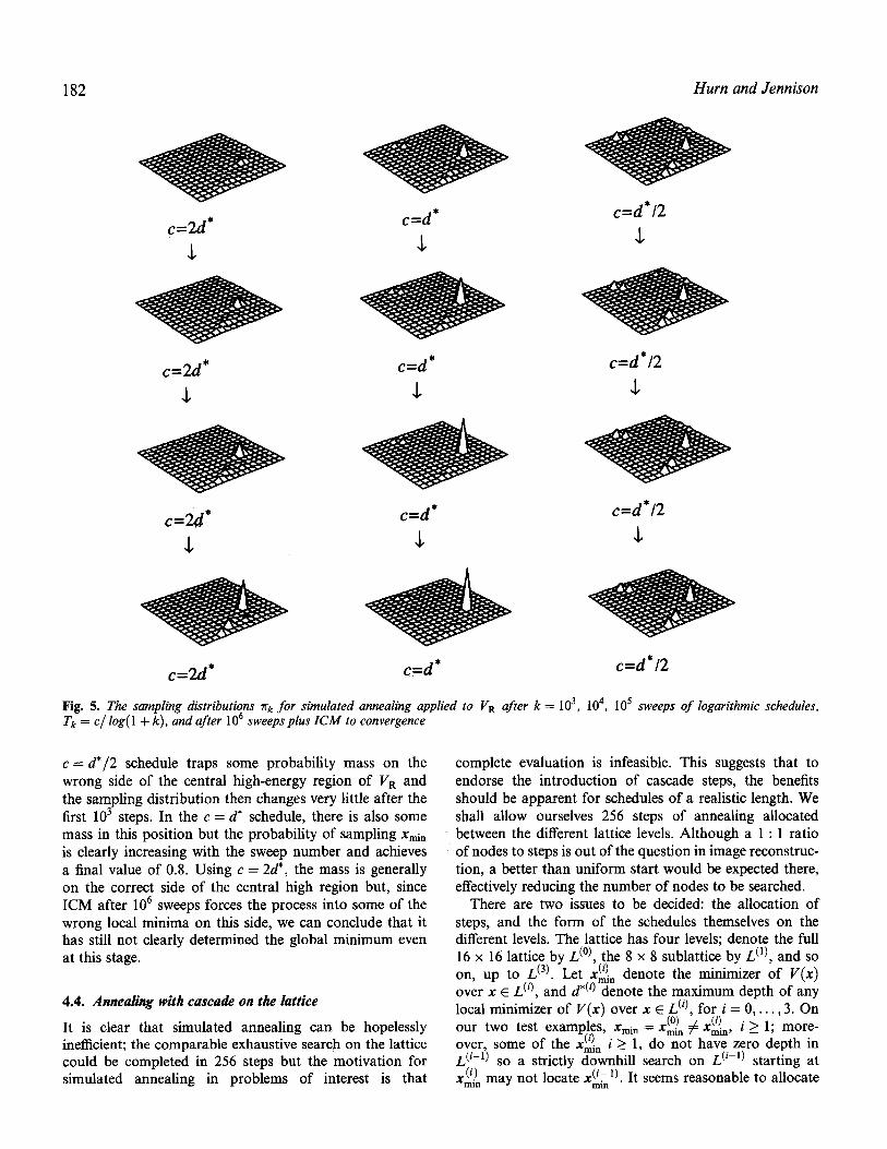
182 Hurn and Jennison
c = 2 d * c=d* c=d* /2 $ $ $
c = 2 d * c=d* c=d* /2 $ $ $
c=2d* c=d* c=d* /2 $ $ $
c = 2 d * c=d* c=d* /2
Fig. 5. The sampling distributions 7r k for simulated annealing applied to V R after k = 10 3, 10 4, 10 5 sweeps of logarithmic schedules, Tk = c~ log(1 + k), and after 10 6 sweeps plus ICM to convergence
c = d*/2 schedule traps some probability mass on the wrong side of the central high-energy region of VR and the sampling distribution then changes very little after the first 10 3 steps. In the c = d* schedule, there is also some mass in this position but the probability of sampling Xmin is clearly increasing with the sweep number and achieves a final value of 0.8. Using c = 2d*, the mass is generally on the correct side of the central high region but, since ICM after 10 6 sweeps forces the process into some of the wrong local minima on this side, we can conclude that it has still not clearly determined the global minimum even at this stage.
4.4. Annealing with cascade on the lattice
It is clear that simulated annealing can be hopelessly inefficient; the comparable exhaustive search on the lattice could be completed in 256 steps but the motivation for simulated annealing in problems of interest is that
complete evaluation is infeasible. This suggests that to endorse the introduction of cascade steps, the benefits should be apparent for schedules of a realistic length. We shall allow ourselves 256 steps of annealing allocated between the different lattice levels. Although a 1 : 1 ratio of nodes to steps is out of the question in image reconstruc- tion, a better than uniform start would be expected there, effectively reducing the number of nodes to be searched.
There are two issues to be decided: the allocation of steps, and the form of the schedules themselves on the different levels. The lattice has four levels; denote the full 16 x 16 lattice by L (~ the 8 x 8 sublattice by L 0), and so
L(3) (,) on, up to . Let x~n denote the minimizer of V(x) over x E L (0, and d *(0 denote the maximum depth of any local minimizer of V(x) over x ~ L (i), for i = 0 , . . . , 3. On our two test examples, X~n = x ~ ) # x~n, i > 1; more- over, some of the x~n i > 1, do not have zero depth in L (~-1) so a strictly downhill search on L (~-0 starting at x(;) may not locate x(g7 l) It seems reasonable to allocate min man "

Simulated annealing and a revised cascade algorithm for image reconstruction 183
the steps unequally as the dimension of the successive minimization problems increases from L (3) to L (0). We have allocated the steps so that the total number of steps completed after annealing on L (0 is proportional to the number of nodes in L (i), i.e. 4 steps on L (3), 12 steps on L (2), and so on. As for schedule form, three types of cas- cade schedule will be compared with a standard non-cas- cade logarithmic schedule followed by ICM, denoted (A). The first cascade schedule, (B), is the sequence of appropri- ate d *(i) standard logarithmic schedules on theL (i), Tk = d*(i)/log(1 + k), wtiere k is the step number within level i. After all but one of the steps allocated to a level have been completed, ICM is applied until convergence and this is counted as the final step. The second, (C), is also logarithmic with ICM at the end of each level but the L (2), L (1) and L (~ schedules are later sections of the same curves; the starting delay is the number of steps already
Temperature schedules
io I ] ~ Cascade logarithmic (B)
50 100 150 200 250
Sweeps
Temperature schedules
<5
i0 50
-- Cascade late logarithmic (C) ....... Standard logarithmic (A)
100 150 200
Sweeps
25O
Temperature schedules
- - Cascade late linear (D) . . . . . . . Standard logarithmic (A)
50 100 150 200 250
Sweeps
Fig. 6. The three cascade schedules which will be used in comparison with the standard non-cascade truncated logarithmic
P(At global minimum)
.s
d i i l ) i l
0 5 0 100 150 2 0 0 2 5 0
Sweeps
Expected energy
o =
m
Standard logarithmic (A)
Cascade logarithmic (B)
Cascade late logarithmic (C)
Cascade late linear (D)
" ...i
�9 i i i i i
0 50 100 150 2 0 0 2 5 0
Sweeps
Fig. 7. Summaries for the three cascade schedules and one non-cas- cade schedule applied to V s
completed, for example during the 48 steps on L (1), the schedule is Tk = d*(1)/log(1 + (16 + k ) ) k = 1 , . . . ,47 and T48 = 0, representing the application of ICM. Cascade schedule (D) is the sequence of linear schedules beginning at the same initial values as the late-start logarithmics (C) and each decreasing to zero. All three schedules for Vs are illustrated in relation to the non-cascade logarithmic schedule in Fig. 6.
We first discuss the results for Vs (see Fig. 7 and Table 1). The success of the schedules is reversed between the two summaries; cascade schedules produce lower expected energies, but lower probabilities of sampling Xmi n. These schedules appear to reach certain non-deleted nodes
Table 1. Final summaries for the four schedules applied to Vs
Expected final Schedule P (Finally at Xmin) energy
Standard logarithmic (A) 0.0531 Cascade logarithmic (B) 0.0398 Cascade late logarithmic (C) 0.0249 Cascade late linear (D) 0.0062
0.0082 0.0081 0.0077 0.0063

184 Hurn and Jennison
of the central low-energy region more rapidly than the non- cascade schedule, hence the rapid drop in expected energy. It seems that on passing from Z (i) to Z (i-1), the two late- start schedules can move out of some of these local minima, incurring the initial increases in expected energy seen in Fig. 7. However, they are already sufficiently cold that they are trapped within the deeper basins, although quite successfully locating low-energy values within these basins. Such behaviour is consistent with the observed low expected energies, but corresponding low probability of sampling Xmi n. The hotter schedule (B) is more mobile, hence the increased probability of sampling Xmi~, and larger rise in expected energy between levels. Unfortu- nately, this schedule suffers from the associated problem of being too hot for a final low expected energy.
Figure 8 and Table 2 demonstrate the advantages of cascade more conclusively for VR. The three cascade schedules produce similar values for the final probability of sampling Xmin, all significantly larger than that of the non-cascade method. VR contains fewer, more distinct, minima than V s, and the increases in expected energy shortly after moving from one level to the next suggest that there is less need for an initial high-temperature phase
P(At global minimum)
d
o. O
I
/ I / t
///// I
i i i i i i
0 50 100 150 200 250
Sweeps
Expected energy
O
Standard logarithmic (A)
........... Cascade logarithmic (B)
.... Cascade late logarithmic (C)
. ~ Cascade late linear (D)
,,~ ~-:.::. - ................................ .~
-- ~" ~ ~ =--~ 2-- . . . . . . . . =':':=':':=i
i i i i i i
0 50 100 150 200 250 Sweeps
Fig. 8. Summaries for the three cascade schedules and one non- cascade schedule applied to VR
Table 2. Final summaries for the four schedules applied to VR
Expected final Schedule P (Finally at Xmin) energy
Standard logarithmic (A) 0.2638 Cascade logarithmic (B) 0.3121 Cascade late logarithmic (C) 0.3221 Cascade late linear (D) 0.3091
0.1708 0.1102 0.0999 0.0905
on the lower levels. The late-start schedules generate the lowest final expected energies, whereas schedule (B) on L (~ appears to undo previous work.
4.5. Conclusions from the lattice problem
The benefits of cascade depend on which of the two perfor- mance measures is more important and on the form of V. Our interpretations of Vs and VR were as a cascade- thinned portion of the energy function and as a magnified low-energy region, respectively. The minimizer of the cas- cade-reduced function is not necessarily the best starting point for minimization on the full energy function but it is plausible that in many cases low-energy states are better starting values. Hence, for Vs we might be more worried about the expected energy than the probability of finding the cascade minimum. However, once in a suitable basin of the energy function, corresponding to VR, we are equally interested in both quantities. Additionally, in the image case, we argued that the expected energy is a more appropriate diagnostic since we can only realistically hope to find a good local minimum. Our conclusion is that the inclusion of cascade steps can be beneficial.
5. An adaptive cascade algorithm for image reconstruction
5.1. Introduction
We now return to the original image reconstruction prob- lem. The intention in applying cascade was to improve the minimization of the energy function without greatly increasing the computational effort. The lattice results suggest that this is achieved by providing a good starting value for processing at the original resolution. However, we have not demonstrated any connection between the minima on different levels of the image problem and here the thinning due to cascade is far more extensive than its lattice analogy equivalent. For the strictly downhill ICM search, the naive grouping of pixels into 2 m x 2 m blocks at one level will not always lead to a helpful starting con- figuration for processing 2 m- 1 • 2 m- l blocks at the next level. Even in the more flexible simulated annealing search, we may do no better using cascade if the successive minima are awkwardly separated in f~. Intuitively we might

Simulated annealing and a revised cascade algorithm for image reconstruction 185
expect the best performance when the blocking at higher cascade levels is allowed to adapt to the record so that blocks consist of pixels whose behaviour suggests some cohesion. In this way, updating a block can produce a coherent large step across 9t and a useful reduction in energy.
5.2. Adaptive and window cascades
We have implemented a scheme for partitioning the image into rectangular blocks of pixels at each cascade level. The same numbers of blocks are retained at successive levels as in the square blocking scheme but the size and shape of these blocks are based on the observed records. For compu- tational simplicity horizontal and vertical partitions are selected independently. In order to choose a good partition of the image, a measure of dissimilarity between pixels lying in separate blocks is required. The obvious measure is the difference between the average records in the blocks on either side of a new partition. Experiments suggest that such a scheme is most effective when the record averages are formed only over strips adjacent to the partition. This approach requires a parameter ~, the width in pixels of these row-wise or column-wise strips. If an existing block boundary is encountered within ~ pixels of a partition the strip is truncated at that point; as the strips may then contain different numbers of pixels, the differences are normalized to have unit variance. For all potential parti- tion sites we form this normalized average record difference and then select the site with the highest absolute difference as the new partition. The cascade of image reconstructions is produced in the same way as pre- viously, proceeding from a single large block down to the individual pixel level. The difference in this adaptive
cascade is that the blocks of pixels constrained to take a common value at each level are those defined by the data- dependent partitions. Again, either ICM or simulated annealing may be used for processing at each cascade level.
Partitions defined for the whole image are unlikely to be optimal for all the small objects or features in an image. To tackle this difficulty, we propose a scheme in which an initial image estimate is produced and small regions of this image are then updated, one by one. When updating a chosen region, or window, all pixel values outside the window are held fixed, and a new reconstruction is obtained within the window using the adaptive cascade algorithm on these pixels alone. The cascade is initialized with the average current grey level within the window and blocks are then updated in the usual way using all relevant pixel values and records. If the new reconstruction within the window leads to a decrease in energy for the entire scene, it is retained; if not, the previous values of the window pixels are restored. We use a square window shifted across the grid with a fixed number of columns over- lapping the previous location; after reaching the right-hand edge of the image, the window is moved back to the left and lowered with a fixed number of rows overlapping its pre- vious vertical location and the process is repeated. In terms of f~, cascade within a window is searching the smaller restricted space determined by the fixed pixel values out- side the window.
Figure 9(a) shows a test image (for display purposes only, the image has been slightly rescaled to provide better con- trast). Eight of the 16 foreground objects, which all take a grey level of 40 in a background of value 20 in the uncor- rupted data, are aligned to 'fit' the original 2 m • 2 m square blocking scheme used by cascade in that they coincide with
Fig. 9. (a) 64 x 64 test image with 64 grey levels; (b) record after 3 • 3 uniform blur and N(0, 1) noise

186 Hurn and Jennison
2 x 2 pixel blocks in the cascade sequence. The remaining eight objects are displaced by one pixel in both directions. Figure 9(b) shows the record obtained by applying a 3 • 3 uniform blur and adding N(0, 1) noise to the true image. In trying to reconstruct the original image, we have used the four nearest neighbour, first-order prior model suggested by Geman and Reynolds (1992):
�9 (x) = ~--~(49/9)(1 + Ixs - xt]/lO) -1 (14) (~,t>
The value 10 in equation (14) represents a typical grey-level discontinuity expected in the image. The factor 49/9 in ~( ) arises from setting Geman and Reynolds' parameter d equal to 3, a value they recommend. (We refer the reader to Geman and Reynolds' paper for a fuller discussion of this model.) Using this prior, the true image has energy 429.9.
All reconstruction methods were initialized with values xs equal to the record associated with pixel s, or the nearest record for pixels s at the image boundary. Single-site ICM achieved an energy of 487.2, non-adaptive cascade ICM working down from a single large block to individual pixels achieved an energy of 454.0, while a realization of single-site simulated annealing using the Gibbs sampler with temperature decreasing linearly from 1 to 0 in 100 sweeps achieved energy 436.6. The simulated annealing took approximately 20 times more computational effort as measured by CPU time than both ICM methods. Using the outlined adaptive partitioning of the entire image with
= 2 and ICM at each cascade level resulted in the recon- struction shown in Fig. 10(a), which has energy 451.7. Clearly the structure of the image meant that the partition- ing scheme was inadequate, and the deterministic ICM was unable to overcome this. However, taking this recon- struction as a starting value and using just the window illustrated in Fig. 10, an energy reduction was achieved to 448.4 from 451.7. The final reconstruction after complete coverage of the grid by overlapping windows had energy 433.3. This energy is lower than the simulated annealing solution, but required only a fraction of the CPU time; the cost of a complete window cascade sweep of the grid was approximately that of an entire grid cascade. If the windows were non-overlapping, then the work involved would be roughly equivalent to a complete grid cascade starting at the level of aggregation defined by the window size. However, the additional work incurred by the overlapping blocks is offset by the saving in not processing the higher cascade levels. It is worth noting that the adaptive window cascade can be implemented easily by minor modifications to an adaptive cascade program.
The windowing idea can help compensate for the limita- tions of a particular partitioning scheme, in that the grid can be swept sequentially with a number of different
schemes. We have experimented with varying ~ within the scheme described so far, and also with an analogous diagonal partitioning scheme which is effective in reconstructuring diagonal object boundaries. There is considerable flexibility in what can be done.
5.3. A synthetic aperture radar ( SAR) example
The data shown in Fig. 1 l(a) form a 128 x 128 pixel section of a larger SAR image of an area near Thetford Forest, England, obtained by plane as part of the Maestro-1 campaign during August 1989. The data were made avail- able by Dr E. Attema of the European Space Research and Technology Centre, Netherlands. Although the image is not blurred, it is heavily degraded by noise, the speckle noise is estimated to have a variance of 202.5 on 256 possible grey levels (for details see Horgan, 1994). The Geman and Reynolds (1992) prior has again been used, this time with eight neighbours and parameters d = 3 and A = 40 (increased to reflect the larger number of grey levels). Hum and Jennison (1994) give details of the extension of the parameter selection required for eight neighbours, and in this case
if(x) = ~ 6.86(1 + Ixs - xtl/40) -1 (15) (s,t>
In Figs 1 l(b)-(e) we show reconstructions of the image obtained using four approaches: single-site ICM, ICM window cascade, single-site simulated annealing and adaptive cascade simulated annealing. We have found that, if good results are to be obtained, window cascade must be used in conjunction with ICM in order to compen- sate for its sensitivity to the starting configuration. The more robust simulated annealing shows substantial improvement from the less computationally demanding adaptive cascade. The ICM window cascade is initialized at the single-site ICM solution and permitted two different window schemes in turn. These two sets of windows both use the parameter
= 2 (window size 16 • 16 with an overlap of 4 pixels in both directions) either with a horizontal-vertical or with a diagonal partitioning scheme. For the single-site Gibbs sam- pler annealing, the schedule descends linearly from 1 to 0 in 100 sweeps. The adaptive cascade schedule, the late-start linear form described as (D) in Section 4.4 which worked well for the lattice, has been matched to this in length and initial temperature. On the lattice, we divided the sweeps between the levels in proportion to the size of the newly introduced space to be searched; this is not reasonable in the image problem where the cascade thinning is much more pronounced. However, it might be argued that we have a better than uniform starting image and the accepta- ble images, those with comparatively low energy, are clus- tered in regions which grow more slowly in dimension

Simulated annealing and a revL~ed cascade algorithm for image reconstruction 187
Fig. 10. The stages of one adaptive window cascade with ~ = 2for the simulated data. (a) Adaptive cascade reconstruction; energy 451.7. ( b ) Average pixel value within particular window. ( c ) Reconstruction at third level showing adaptive partitions. ( d) Reconstruction at second level showing adaptive partitions, (e) Reconstruction at first level showing adaptive partitions. (f) Final reconstruction; energy 448.4

188 Hurn and Jennison
Fig. 11. The SAR data and four reconstructions. (a) 128 x 128 data. (b) Single-site ICM; energy 3381.3. (e) Window cascade ICM; energy 2642.7. (d) Single-site annealing; energy 2902.8. (e) Adaptive cascade annealing; energy 2722.8

Simula ted annealing and a revised cascade algorithm fo r image reconstruction 189
than does the entire set of attainable images. As a result, we have judgementally allocated sweeps to different levels roughly in proportion to the increase in the number of cas- cade blocks, rather than the number of attainable images. The inclusion of some form of cascade step has resulted in a reduction in energy whether using ICM or simulated annealing (the energy values are given in Fig. 11). In order from lowest to highest energies, the reconstructions are win- dow cascade ICM, adaptive cascade annealing, single-site annealing and single-site ICM.
In this SAR example, the data are sufficiently noisy that the image is not particularly easy to interpret by eye and one aim of reconstruction is to provide a clearer summary of the main features of the image. Other objectives in analysing data of this type could include a numerical assess- ment of land usage. In addition to providing reconstruc- tions with low energies, we believe the ICM window cascade and adaptive cascade simulated annealing produce visually satisfactory images, and the first of these offers particular promise for use in pixel classification or image segmentation.
6. Summary
MAP image reconstruction necessitates a very high- dimensional optimization. This problem is usually tackled with either the slow, stochastic algorithm simulated annealing or the fast but generally inferior ICM approach; simulations suggest that even the more accurate simulated annealing can perform very badly, particularly under a poor choice of temperature schedule. Multiple- site updating, moving in large steps around the objective function, is seen as a means to improve performance, but in practice it is hard to formulate in a computationally feasible way. We have modified and extended the very simple cascade algorithm, which implements certain multiple-site updates by blocking similar components together. Results suggest that this cascade can dramati- cally improve the minimization performance with little extra computational burden. This concept of large, coherent steps in the minimization process may well be of value in many other large-scale optimization problems with multiple local optima: such problems arise in a host of industrial applications ranging from micro-chip design to the scheduling of flexible assembly lines and the optimal use of materials in fabrication and manufacturing.
Acknowledgements
We are grateful to the referees for their constructive criti- cism. Merrilee Hurn was funded by a Science and Engineer- ing Research Council studentship.
References
Amit, Y. and Grenander, U. (1991) Comparing sweep strategies for stochastic relaxation. Journal of Multivariate Analysis, 37, 197-222.
Besag, J. (1986) On the statistical analysis of dirty pictures (with discussion). Journal of the Royal Statistical Society B, 48, 259-302.
Edwards, R. and Sokal, A. (1988) Generalization of the Fortuin- Kasteleyn-Swendsen-Wang representation and Monte Carlo algorithm. Physical Review D, 38, 2009-2012.
Geman, D. (1990) Random Fields and Inverse Problems in Imaging. Lecture Notes in Mathematics, Springer-Verlag, Berlin.
Geman, S. and Geman, D. (1984) Stochastic relaxation, Gibbs distributions, and the Bayesian restoration of images. IEEE Transactions on pattern Analysis and Machine Intelligence, PAMI-6, 721 741.
Geman, D. and Reynolds, G. (1992) Constrained restoration and the recovery of discontinuities. IEEE Transactions on Pattern Analysis and Machine Intelligence, PAMI-14, 367-383.
Geyer, C. (1991) Markov chain Monte Carlo maximum likeli- hood. In Computer Science and Statistics, Proceedings of the 23rd Interface (ed. Keramidas, P.), pp. 156 163. Inter- face Foundation, Fairfax Station.
Gidas, B. (1989) A renormalisation group approach to image processing problems. IEEE Transactions on Pattern Analysis and Machine Intelligence, PAMI-11, 164-180.
Greig, D., Porteous, B. and Seheult, A. (1989) Exact maximum a posteriori estimation for binary images. Journal of the Royal Statistical Society B, 51, 271-279.
Hajek, B. (1988) Cooling schedules for optimal annealing. Mathe- matics of Operational Research, 13, 311-329.
Hastings, W. (1970) Monte Carlo sampling methods using Markov chains and their applications. Biometrika, 57, 97- 109.
Horgan, G. (1994) Choosing weight functions for filtering SAR. International Journal of Remote Sensing, to appear.
Hurn, M. (1994) An Adaptive Swendsen and Wang Type Algorithm. Technical Report 94:03, University of Bath, UK.
Hurn, M. and Jennison, C. (1994) An Extension of Geman and Reynolds' Approach to Constrained Restoration and the Recover), of Discontinuities. Technical Report 94:02, Univer- sity of Bath, UK.
Jubb, M. and Jennison, C. (1991) Aggregation and refinement in binary image restoration. In: Spatial Statistics and Imaging (ed. Possolo, A.), pp. 150-162. Institute of Mathematical Sciences Lecture Notes, Hayward, CA.
Kirkpatrick, S., Gelatt, C. and Vecchi, M. (1983) Optimization by simulated annealing. Science, 22, 671-680.
Marroquin, J., Mitter, S. and Poggio, T. (1987) Probabilistic solution of ill-posed problems in computational vision. Journal of the American Statistical Association, 82, 76 89.
Metropolis, N., Rosenbluth, A., Rosenbluth, M., Teller, A. and Teller, E. (1953) Equations of state calculations by fast computing machines. Journal of Chemical Physics, 21, 1087-1092.
Peskun, P. (1973) Optimum Monte Carlo sampling using Markov chains. Biometrika, 60, 607 612.

190 Hum and Jennison
Ripley, B. (1988) Statistical Inference for Spatial Processes. Cambridge University Press, Cambridge.
Rue, H. (1994) New Loss Functions in Bayesian Imaging. Technical Report, Department of Mathematical Sciences, Norwegian Institute of Technology, Trondheim.
Sokal, A. (1989) Monte Carlo Methods in Statistical Mechanics:
Foundations and New Algorithms. Cours de Troisi6me Cycle de la Physique en Suisse Romande, Lausanne.
Swendsen, R. and Wang, J. (1987) Nonuniversal critical dynamics in Monte Carlo simulations. Physical Review Letters, 58, 86- 88.