a study of electrogenic transient and steady-state ... a study of electrogenic transient and...
TRANSCRIPT

A Study of Electrogenic Transient and Steady-State Cotransporter Kinetics: Investigations with the
Na+/Glucose Transporter SGLT1
by
Daniel Krofchick
A thesis submitted in conformity with the requirements for the degree of Doctor of Philosophy
Institute of Medical Science University of Toronto
© Copyright by Daniel Krofchick 2012

ii
A Study of Electrogenic Transient and Steady-State
Cotransporter Kinetics: Investigations with the Na+/Glucose
Transporter SGLT1
Daniel Krofchick
Doctor of Philosophy
Institute of Medical Science
University of Toronto
2012
Abstract
Significant advancements in the field of membrane protein crystallography have provided in
recent years invaluable images of transporter structures. These structures, however, are static
and require complementary kinetic insight to understand how their mechanisms work.
Electrophysiological studies of transporters permit the high quality kinetic measurements
desired, but there are significant difficulties involved in analyzing and interpreting the data.
Current methods allow a variety of kinetic parameters to be measured but there is a disconnect
between these parameters and a fundamental understanding of the carrier. The intent of this
research was to contribute new tools for studying the electrogenic kinetics of membrane
transport proteins, to understand the link between these kinetics and the carrier, and to
ultimately understand the mechanisms involved in transport. In this vein, two projects are
explored covering two important kinetic time domains, transient and steady-state. The transient
project studies the conformational changes of the unloaded carrier of SGLT1 through a multi-
exponential analysis of the transient currents. Crystal structures have potentially identified a
gated rocker-switch mechanism and the transient kinetics are used to support and study this
kinetically. A protocol taking advantage of multiple holding potentials is used to measure the

iii
decay time constants and charge movements for voltage jumps from both hyperpolarizing and
depolarizing directions. These directional measurements provide insight into the arrangement of
the observed transitions through directional inequalities in charge movement, by considering the
potential for a slow transition to hide a faster one. Ultimately, four carrier decays are observed
that align with the gated rocker-switch mechanism and can be associated one-to-one with the
movement of a gate and pore on each side of the membrane. The steady-state project considers a
general theoretical model of transporter cycling. Recursive patterns are identified in the steady-
state velocity equation that lead to a broad understanding of its geometric properties as a
function of voltage and substrate concentration. This results in a simple phenomenological
method for characterizing the I–V curves and for measuring the kinetics of rate limiting patterns
in the loop, which we find are the basic structures revealed by the steady-state velocity.

iv
Acknowledgments
To my grandparent, who began this journey with me and are no longer here. My parents, who’s
support and love kept me going. And most of all Kate, who made this all possible.

v
Table of Contents
Acknowledgments .......................................................................................................................... iv
Table of Contents ............................................................................................................................. v
List of Tables ................................................................................................................................... x
List of Figures ................................................................................................................................. xi
List of Abbreviations .................................................................................................................... xiv
List of Variables ............................................................................................................................ xv
Introduction ................................................................................................................................. 1 1
1.1 Types of Transport ............................................................................................................... 4
1.1.1 Facilitated Diffusion ................................................................................................ 4
1.1.2 Primary Active Transport ........................................................................................ 5
1.1.3 Secondary Active Transport .................................................................................... 5
1.2 Familial Relations of SGLT1............................................................................................... 6
1.2.1 SLC5 Family ............................................................................................................ 7
1.2.2 The Solute:Sodium Symporter Family .................................................................. 12
1.2.3 Phylogenetic Homology ........................................................................................ 12
1.2.4 Structural Homology ............................................................................................. 13
1.2.5 Figures ................................................................................................................... 15
1.3 Crystal Structures of the LeuT Fold .................................................................................. 19
1.3.1 Timeline ................................................................................................................. 19
1.3.2 Architecture ........................................................................................................... 20
1.3.3 Solved Conformations ........................................................................................... 20
1.3.4 Pores ...................................................................................................................... 21
1.3.5 Thin Gates .............................................................................................................. 22

vi
1.3.6 Substrate Site ......................................................................................................... 23
1.3.7 Cation Sites ............................................................................................................ 24
1.3.8 Inhibitor Sites......................................................................................................... 25
1.3.9 Thick Gates ............................................................................................................ 26
1.3.10 Conformational Changes ....................................................................................... 27
1.3.11 Transport Model .................................................................................................... 28
1.3.12 Figures ................................................................................................................... 29
1.4 Rationale ............................................................................................................................ 40
Dissecting the Transient Current of SGLT1 ............................................................................. 43 2
2.1 Introduction........................................................................................................................ 43
2.1.1 The T156C Mutant ................................................................................................ 45
2.1.2 Historical Perspective ............................................................................................ 46
2.1.3 This Study .............................................................................................................. 49
2.2 Materials an Methods ........................................................................................................ 50
2.2.1 Molecular Biology ................................................................................................. 50
2.2.2 Oocyte Collection, Injection, and Maintenance .................................................... 50
2.2.3 Two-Electrode Voltage-Clamp .............................................................................. 51
2.2.4 Voltage-Clamp Protocol ........................................................................................ 51
2.2.5 Exponential Curve Fitting...................................................................................... 52
2.3 Voltage Jump Experiment Theory ..................................................................................... 53
2.3.1 Anatomy of a Voltage Jump .................................................................................. 53
2.3.2 The Transient ......................................................................................................... 53
2.3.3 How the Voltage Jump Affects the Transient........................................................ 54
2.3.4 How the System Affects the Transient .................................................................. 54
2.3.5 Voltage Jump Protocols ......................................................................................... 55
2.4 Data Analysis ..................................................................................................................... 56

vii
2.4.1 Form of the Transient Currents ............................................................................. 56
2.4.2 Defining the Data Set............................................................................................. 56
2.4.3 Fitting ..................................................................................................................... 57
2.4.4 Fit Quality: Residuals and χ2 ................................................................................. 58
2.4.5 Nonsense Fits ......................................................................................................... 58
2.4.6 Seeding .................................................................................................................. 59
2.4.7 Stopping ................................................................................................................. 61
2.4.8 Parameter Variation with the Number of Terms ................................................... 61
2.4.9 Looking at the Dataset as a Whole ........................................................................ 62
2.5 Results ............................................................................................................................... 63
2.5.1 Transient Kinetics of wt and the T156C mutant .................................................... 63
2.5.2 Capacitive Decay ................................................................................................... 63
2.5.3 Carrier Decays: Charge Movements ...................................................................... 64
2.5.4 Carrier Decays: Time Constants ............................................................................ 64
2.5.5 Phloridzin and Non-Injected Controls ................................................................... 65
2.5.6 Limiting Terms and its Effect on the Measured Kinetics ...................................... 65
2.5.7 Using Expected Behavior to Predict the Number of Terms .................................. 66
2.5.8 Dependence of the Decay Charges on the Holding and Test Potentials................ 67
2.5.9 Supplementary Data............................................................................................... 68
2.6 Discussion .......................................................................................................................... 68
2.6.1 Ordering the Transitions ........................................................................................ 68
2.6.2 Carrier Conformations ........................................................................................... 69
2.6.3 Functional Insights................................................................................................. 70
2.6.4 Building a Kinetic Model ...................................................................................... 71
2.7 Summary and Conclusion .................................................................................................. 71
2.8 Future Work ....................................................................................................................... 73

viii
2.8.1 Simulations ............................................................................................................ 73
2.8.2 Strategic Mutants ................................................................................................... 74
2.8.3 Substrate Transients ............................................................................................... 76
2.8.4 Other Carriers and Mechanisms ............................................................................ 76
2.8.5 Miscellaneous ........................................................................................................ 78
2.9 Figures ............................................................................................................................... 79
A Practical Method for Characterizing the Voltage and Substrate Dependence of 3
Membrane Transporter Steady-State Currents........................................................................ 101
3.1 Introduction...................................................................................................................... 101
3.1.1 Historical Perspective .......................................................................................... 102
3.1.2 This Study ............................................................................................................ 104
3.2 Steady-State Velocity of a Cyclical Model ..................................................................... 105
3.3 Voltage Dependence ........................................................................................................ 106
3.3.1 Introducing Voltage Dependence ........................................................................ 106
3.3.2 The General Voltage Dependent Equation .......................................................... 108
3.3.3 Geometric Properties of the I–V Curves ............................................................. 110
3.4 Substrate Dependence ...................................................................................................... 112
3.4.1 Introducing Substrate Dependence ...................................................................... 112
3.4.2 Characteristics of Substrate Dependence............................................................. 113
3.5 Results ............................................................................................................................. 115
3.5.1 Characterizing Experimental Data ....................................................................... 115
3.5.2 Modeling the Steady-State Velocity .................................................................... 116
3.6 Summary and Conclusion ................................................................................................ 118
3.7 Future Work ..................................................................................................................... 119
3.8 Appendix.......................................................................................................................... 120
3.8.1 Deriving and Arranging the Steady-State Equation ............................................ 120
3.8.2 Simplifying the Voltage Dependent Expressions ................................................ 121

ix
3.8.3 Simplifying the Substrate Dependent Expression ............................................... 123
3.8.4 Two Substrate Binding Events ............................................................................ 124
3.9 Figures ............................................................................................................................. 126
Conclusion and Future Work .................................................................................................. 138 4
References.................................................................................................................................... 140

x
List of Tables
Table 1: Properties of SLC5 and select TC 2.A.21 members ........................................................ 15
Table 2: Properties of the LeuT fold transporters .......................................................................... 29
Table 3: Gate, substrate and cation interacting residues for the LeuT fold transporters ............... 30
Table 4: Nonsense fit examples ..................................................................................................... 88
Table 5: Seeding examples for multi-exponential fitting .............................................................. 89
Table 6: Example voltage dependent map of a transient kinetics exponential fit analysis. .......... 91

xi
List of Figures
Fig. 1: Classical SGLT1 transport model ...................................................................................... 16
Fig. 2: Homology of the SLC5 and SSS families .......................................................................... 17
Fig. 3: Phylogenic tree of secondary active transport families with solved crystal structures ...... 18
Fig. 4: Timeline of discovery for the LeuT fold structures ........................................................... 31
Fig. 5: Organization of the TM segments for the LeuT fold structures ......................................... 32
Fig. 6: Extracellular and intracellular pores demonstrated by LeuT, BetP and vSGLT ................ 33
Fig. 7: Gating mechanisms ............................................................................................................ 34
Fig. 8: Substrate binding site ......................................................................................................... 35
Fig. 9: Cation binding sites ............................................................................................................ 36
Fig. 10: LeuT with multiple bound substrates ............................................................................... 37
Fig. 11: Competitive and non-competitive inhibitor binding sites in LeuT .................................. 38
Fig. 12: Transport model predicted by the various conformations of the LeuT architecture
captured in crystal structures ......................................................................................................... 39
Fig. 13: Characteristics of the T156C mutant ................................................................................ 79
Fig. 14: Position of the T156 and K157 residues of SGLT1 in the vSGLT structure ................... 80
Fig. 15: Anatomy of a voltage jump .............................................................................................. 81
Fig. 16: Relationship between voltage jumps and transient kinetics ............................................. 82
Fig. 17: Hypothetical three-state system illustrating the masking effect....................................... 83
Fig. 18: Single and multi-holding voltage clamp protocols .......................................................... 84
Fig. 19: Example multi-holding data set........................................................................................ 85
xii
Fig. 20: Multi-exponential fit of a transient data set ..................................................................... 86
Fig. 21: Fit residuals ...................................................................................................................... 87
Fig. 22: Transient charge movements by component .................................................................... 90
Fig. 23: Transient kinetics of SGLT1 ............................................................................................ 92
Fig. 24: An expanded overview of the transient kinetic data ........................................................ 93
Fig. 25: Close up of the transient kinetic data ............................................................................... 94
Fig. 26: Changes in measured kinetics when fitting with limited exponential terms .................... 95
Fig. 27: Component charge dependence on the holding and test potential ................................... 96
Fig. 28: Additional wt and T156C transient kinetic data sets........................................................ 97
Fig. 29: Arranging decay charge profiles using the masking effect .............................................. 98
Fig. 30: Assigning transient decays to conformational changes of the carrier predicted by the
crystal model .................................................................................................................................. 99
Fig. 31: Revised SGLT1 transport model ...................................................................................... 99
Fig. 32: Rough state-model of SGLT1 transport ......................................................................... 100
Fig. 33: Types of time constant voltage dependent behavior ...................................................... 100
Fig. 34: Example I–V data ........................................................................................................... 126
Fig. 35: General -state cyclical model ....................................................................................... 127
Fig. 36: Example showing the form of the steady-state equation ............................................... 128
Fig. 37: Example 1. Solution of the voltage dependent general velocity equation ..................... 129
Fig. 38: Geometric properties of a sigmoid function ................................................................... 129
Fig. 39: Effect of a dominant denominator term ......................................................................... 130
xiii
Fig. 40: Geometric properties of a sigmoid function with two terms .......................................... 131
Fig. 41: Example 2. Voltage dependent properties of the general velocity equations ................ 132
Fig. 42: Characteristics of the logarithmic exponential shifts ..................................................... 133
Fig. 43: Example 3. Substrate dependence of the I–V curves ..................................................... 134
Fig. 44: Analyzing experimental I–V data .................................................................................. 135
Fig. 45: Steady-State velocity models ......................................................................................... 136
Fig. 46: Voltage dependence of the Na+ and αMG apparent affinities for the Q170C and Q170E
mutants of rSGLT1 ...................................................................................................................... 137
xiv
List of Abbreviations
AdiC arginine/agmatine antiporter
AcrB multidrug efflux transporter
APC amino acid-polyamine-organocation family
ApcT H+/amino-acid symporter
BCCT betaine/carnitine/choline transporter family
BetP Na+/betaine transporter
CHT Na+/choline transporter
EmrD multidrug efflux pump
EmrE multidrug efflux pump
GlpT glycerol-3-phosphate/Pi exchanger
K157C lysine to cysteine mutant of SGLT1
LacY lactose permease
LeuT Na+/leucine transporter
MFS major facilitator superfamily
Mhp1 Na+/benzyl-hydantoin transporter
NCS1 nucleobase cation symporter-1 family
N Na+
NIS Na+/iodide symporter
NSS neurotransmitter:sodium symporter family
OxlT oxalate/formate exchanger
PutP Na+/proline transporter
Pz phloridzin
RND resistance nodulation-cell division superfamily
S sugar, glucose, phloridzin
SGLT(1–5) Na+/glucose transporter
SMCT(1–2) Na+/monocarboxylate transporter
SMIT(1–2) Na+/myo-inositol transporter
SMVT Na+/multivitamin transporter
SSS(F) solute:sodium symporter family
T156C threonine to cysteine mutant of SGLT1
TC transport classification system
TCA tricyclic antidepressant
TM transmembrane segment
vSGLT Vibrio parahaemolyticus Na+/galactose transporter

xv
List of Variables
amplitude
( )⁄
capacitance
elementary charge
Faraday constant
current
, sum of voltage and substrate independent snake terms
dissociation constant for transition
, coefficient of substrate dependent snake term
,
coefficient of voltage dependent snake term
,
coefficient of voltage and substrate dependent snake term
Michaelis-Menten apparent affinity
, voltage independent factor of a voltage dependent rate constant
, rate constants for transition
number of expressed carrier proteins
Hill coefficient
charge,
net charge translocated per cycle
gas constant
net steady-state velocity,
, steady-state velocities
, maximum steady-state velocity
substrate, substrate concentration
absolute temperature
time constant
reduced voltage, ( )⁄
, exponential shift of voltage dependent snake term
,
exponential shift of voltage and substrate dependent snake term
, voltage
, voltage at half maximum amplitude, ( ( ))⁄
holding potential
Michaelis-Menten maximum velocity
resting potential
at saturating substrate concentrations for I–V curves
test potential
valence
, combined valence of voltage dependent snake term
,
combined valence of voltage and substrate dependent snake term
1
Introduction 1
Secondary active transport was first proposed by Robert Crane in 1960 to explain the uphill
transport of glucose and other molecules in the intestinal brush border. He hypothesized that the
translocation of substrate was coupled to Na+, which would energize this process through the
Na+ gradient maintained by the Na
+/K
+ pump
1. This mechanism was clarified a few years later
in 1966 when Jardetzky outlined an hypothesis whereby transport could occur through
alternating access to a central substrate binding site2. Throughout the 60’s and 70’s research was
focused on determining substrate and ion specificity of sugar and amino acid absorption using in
vitro preparations of various intact tissues and radioactive tracers3. Although much work at this
time focused on kinetic studies, and theoretical derivations, the available techniques posed
significant difficulties (unstirred layers, cell metabolism of the substrate, multiple endogenous
transport pathways, and an uncontrolled membrane potential) that limited the precision of the
measurements and depth of analysis.
A significant advancement was the use of isolated membrane vesicles, initially prepared from E.
coli (1966)4, and later adapted to the brush border (1973)
5. This new technique solved a number
of concerns and allowed for much more control over the experimental conditions, including
limited manipulation of the membrane potential6,7
. For the most part, these studies involved
steady-state and equilibrium measurements with radiotracers that led to more precise
characterization of affinities and coupling ratios. However, the presence of heterologous
transport pathways remained a major drawback that complicated kinetic analysis8.
Expression cloning, originally demonstrated with rabbit SGLT1 in 19879, marked a new era in
the study of membrane transport10,11. For the first time, carrier proteins could be cloned and
studied in a heterologous system. Not only were the majority of earlier complications resolved,
but a new powerful and precise tool became available for controlling and monitoring these
proteins. The two-electrode voltage-clamp and the oocyte system brought electrophysiological
techniques to secondary active transporters, whose expression levels and currents are too small
to observe with the patch clamp in native tissues (turnover of ~10 s−1
for carriers12
versus ~200
s−1
for pumps and ~106–10
8 s
−1 for channels
13,14). Soon apparent affinities, turnover rates, and
coupling ratios (and their voltage dependencies) were being measured in greater detail than ever

2
before. In addition, rapid transient studies became possible, allowing for measurement of
expression level, valences, ’s, decay time constants and amplitudes.
Once cloning was available, mutation studies became a popular means of studying the
relationship between structure and function, and often these mutants were characterized in the
oocyte system with electrophysiological techniques. Our group used cysteine scanning
mutagenesis to identify a region of SGLT1 critical for substrate binding (K157, T156)15-17
,
while others found a key residue in translocation (Q457)18
, and a structurally significant
disulfide bridge (C255–C511)19
.
Progress in elucidating mechanism, however, was tempered by the sheer difficulty of inferring
potentially complex interactions without a tertiary structure. Much of these kinetic studies
supported the alternating access hypothesis proposed by Jardetzky, but none were able to verify
it. However, as discussed in §1.3 Crystal Structures of the LeuT Fold, this began to change in
2008 when the crystal structure of a bacterial Na+/galactose transporter (vSGLT) was solved, a
homolog of SGLT1. Quite surprisingly, the vSGLT architecture was found to be the same as the
leucine transporter (LeuT), which shares no sequence similarity and has two fewer
transmembrane domains. In the years that followed, this structural superfamily has grown to
contain members from five genetically distinct transporter families. Furthermore, as these
structures have appeared they have been found in various conformations that sketch out a series
of potential conformational changes involved in transport. These conformational changes have
finally demonstrated the existence of the alternating access mechanism, and in the case of the
LeuT architecture it has become known more specifically as a gated rocker-switch. However,
even with this invaluable structural detail a real limitation is the static nature of these crystals,
and it seems that kinetic studies may be the crucial piece needed to understand the moments in
between, and confirm the gated rocker-switch kinetically.
The goal of this project has been to find ways to extract as much kinetic information as possible
from electrophysiological kinetic studies of cotransporters, to help interpret the crystallographic
data and understand the transport mechanism. Although significant work has been done already
with transient and steady-state studies, the results are often kinetic parameters that help
characterize transporters ( , , , , ), yet fall short of revealing a definitive model. The
models that have been built are often over parameterized, because of insufficient kinetic features

3
and the inherent difficulty of the problem. For decades kinetic studies have progressed in the
dark, but now with the availability of crystal structures it is important to reinvest in this basic
research to take advantage of new synergies that have become available.
The experiments performed in this study are based around the two-electrode voltage-clamp
technique and the heterologous Xenopus laevis (African clawed frog) oocyte expression system.
Protein is overexpressed in the oocytes, and then manipulated and monitored via the membrane
potential by the two electrodes. This research studies two time domains of cotransporter
membrane currents, transient and steady-state, with SGLT1 as a model system; SGLT1’s
properties are discussed in more detail in §1.2.1.1 Sugar: SGLT1–4. Each domain provides
information on different aspects of transport, and both are needed for a complete picture. The
transient currents contain detailed information on individual conformational changes of the
empty carrier, while the steady-state currents measure lumped parameters from the transport
loop. As we will show in §2 Dissecting the Transient Current of SGLT1, the transient currents
of SGLT1 can be decomposed into four carrier decays that reveal the gated-rocker switch
mechanism. Measuring and fitting transient currents is not an easy task, and so we present new
methods for analyzing them in as much detail as possible. What we find is that when all the
decay components are identified it is much easier to build a kinetic model. The steady-state
project presented in §3 A Practical Method for Characterizing the Voltage and Substrate
Dependence of Membrane Transporter Steady-State Currents, uses the concept of a general
cyclical system to model the voltage and substrate dependence of the steady-state velocity.
Recursive patterns in the velocity equation allow for a general understanding of its geometric
features. This reveals that the I–V curves can be modeled phenomenological with Boltzmann
functions whose parameters report on the kinetics of rate limiting segments of the transport
loop. These rate limiting segments hide other parts of the loop and are the most we can hope to
extract from steady-state studies. Only by combining the strengths of transient and steady-state
studies with crystallographic research can we complete the picture of how transporters work.
Although most of this research is centered around SGLT1, this carrier is an excellent model
system for ion-coupled cotransporters and these results can be extended to many others.

4
1.1 Types of Transport
The flow of molecules across biological membranes is mediated by three major classes of
intrinsic membrane proteins known as channels, pumps, and cotransporters, which comprise
~3% of all protein encoding genes. These classes of carrier proteins are differentiated based on
the size of the molecules they transport, the energy source that drives them, and their basic
architecture and mechanism. On the surface of each cell a diverse ecosystem of hundreds of
these proteins work together to maintain homeostasis, although the size and composition of this
ecosystem can vary considerably between organisms to suit their different needs as shown
below20
:
transport genes channels pumps cotransporters
Human 754 43% 11% 44%
E coli 354 4% 20% 66%
Asian rice 1200 15% 21% 63%
1.1.1 Facilitated Diffusion
Facilitated diffusion involves the transport of ions and small molecules down an electrochemical
gradient. These proteins are not directly coupled to an energy source, and instead rely on other
membrane proteins to maintain the electrochemical gradient that allows them to function.
Because of this they are unable to concentrate their substrate.
Ion channels mediate the rapid and selective movement of ions (~106–10
8 s
−1) such as K
+, Na
+,
Ca2+
, and Cl−, and are fundamental to biological processes that require speed, such as neuronal
signaling and muscle contraction. The channels contain a pore, which the ions flow through, and
a gating mechanism, which controls access to the pore and is regulated by the membrane
potential or another substrate. The first channel crystal structure was solved in 1998 for the K+
channel KcsA (homotetramer, 108 amino acids, 2 transmembrane segments—TMs), which won
McKinnon a shared 2003 Nobel Prize in Chemistry14
with Agre for his discovery of the water
channel aquaporin (AQP1) in 199221
, which was crystalized in 200022
(monomer, 269 amino
acids, 6 TMs).

5
Larger molecules like many dietary sugars are rapidly equilibrated (~1200 s−1
23
) by the GLUT
family of uniporters (monomer, ~500 amino acids, 12 TMs). Although the GLUTs have not
been crystalized, several of their distant relatives including LacY have24
, and belong to the same
major facilitator superfamily (MFS). They are thought to share a similar rocker-switch
mechanism, whereby the substrate binding site, located at the center of the protein, is alternately
exposed to either side of the membrane as two symmetrical halves of the protein rock back and
forth23
.
1.1.2 Primary Active Transport
These carriers, also known as pumps, use an energy source, usually ATP or light, to fuel uphill
transport, and are responsible for maintaining the electrochemical ion gradients that drive
channels and cotransporters, including repolarization after an action potential. The Na+/K
+ pump
is the most well-known member because it energizes most animal cells, while the H+ pump fills
a similar role in plants and fungi. The Ca2+
pump SERCA1a from skeletal muscle was the first
high resolution pump crystal, published in 200025
, with the Na+/K
+ 26
and H+ pumps
27 following
in 2007. They are among the most complex transport proteins (monomer, ~1000 amino acids).
The Na+/K
+ pump, for example, has a two part transmembrane module (10 TMs), three
cytoplasmic domains (A, N, and P), and interacts with two extracellular subunits (β and γ). It
functions by switching between two primary conformational states, which have different
affinities for Na+ and K
+, and alternate exposure of the binding sites on either side of the
membrane28
.
The microbial rhodopsin family of transporters, which includes bacteriorhodopsin, use light to
pump H+, and are much smaller than their ATP counterparts (monomer, 250–350 amino acids,
~7 TMs). Bacteriorhodopsin was first crystalized in 199629
.
1.1.3 Secondary Active Transport
Secondary active transporters, also known as cotransporters, are able to concentrate substrate
like pumps, but use the electrochemical ion gradients (often H+ or Na
+) maintained by pumps as
fuel instead of ATP. They transport a wide variety of substrates and are the predominant mode
of entry for most medium and large sized molecules.

6
There are many different families of secondary active transporters, but some prominent
members include the major facilitator superfamily (MFS), the neurotransmitter:sodium
symporter (NSS) family, and the solute:sodium symporter (SSS) family. The first secondary
active transporter to be crystalized, and the last of the three major classes of transporters, was
the bacterial MFS oxalate:formate exchanger OxlT in 2002 (monomer, 418 amino acids, 12
TMs)30
. Since then three other MFS members have been crystalized, all transporting very
different substrates but with the same rocker-switch architecture; the H+/lactose symporter
LacY24
, the glycerol-3-phosphate/Pi exchanger GlpT31
, and the H+/multidrug exchanger EmrD
32.
This has turned out to be a common theme for secondary active transporters, where the bacterial
NSS 2Na+/Cl
−/leucine symporter LeuT (monomer, 513 amino acids, 12 TMs) architecture is
also shared by a diverse group of carriers belonging to five phylogenetically distinct families
that includes the SSS family. The architecture of this structural superfamily is similar to the
MFS transporters, but has additional gates on either side of the membrane to control access to
the intra and extracellular pores, and is referred to as a gated rocker-switch. SGLT1 belongs to
this structural superfamily which will be discussed in more detail in the next section (§1.2).
1.2 Familial Relations of SGLT1
SGLT1 can be considered a member of three families. It is the most well-known of the 12
member solute carrier 5 (SLC5) family of membrane transport proteins, and was the first to be
cloned (SLC5A1)33
. All together there are 51 SLC families formed from the pool of human
genesa. These groupings are based on a minimum of 20–25% sequence similarity with other
members34
. The Transport Classification (TC)b is a more general system, with transporters of all
species grouped according to function and phylogeny35
, and is modeled after the classification
system for enzymes adopted by the Enzyme Commission (EC). Within the TC system SGLT1
belongs to the solute:sodium symporter (SSS) family (TC 2.A.21); sometimes referred to as the
sodium/substrate symporter family (SSF36
or SSSF37
). In more recent years a structural
superfamily has emerged from the crystal structure literature, where SGLT1 and several other
a Curated by the HUGO Gene Nomenclature Committee (HGNC), an extension of the Human Genome
Organization (HUGO).
b Curated by the Saier lab and adopted by the International Union of Biochemistry and Molecular Biology
(IUBMB).

7
phylogenetically distinct members have been found to share a common architecture based on the
LeuT fold (named after its first member, the Na+/leucine transporter). With SGLT1 belonging to
such a diverse group of genetically or structurally similar transport proteins, it is likely that the
methods and conclusions presented in this thesis can be extended to these other members as
well.
1.2.1 SLC5 Family
1.2.1.1 Sugar: SGLT1–4
Properties of the SLC5 proteins are outlined in Table 1. Four members, SGLT1–4, are primarily
aldohexose transporters. This group includes two of the more prominent members of the SLC5
family, SGLT1 and SGLT2. SGLT1 (SLC5A1) is found mainly in the small intestine, but also
in the heart and kidney and to a lesser extent in some other tissues, and is responsible for the
vast majority of dietary glucose and galactose absorbed across the brush border membrane, from
the lumen into enterocytes and ultimately the bloodstream38,39
. SGLT2 (SLC5A2) is found in
many tissues but is highest in concentration in the kidney proximal tubule, where it reabsorbs
glucose from the glomerular filtrate preventing its loss in the urine38,40,41
. Of these two
transporters, SGLT1 has a high affinity for glucose, 0.5 mM, and couples two Na+ ions to the
transport process42. While SGLT2 is a low affinity transporter, 1.6 mM, that couples a single
Na+ ion.
Defective mutations in SGL1 lead to glucose-galactose malabsorption, a rare autosomal
recessive disease. The disease appears in newborn infants as diarrhea and dehydration, which is
ultimately fatal unless all glucose, galactose, and lactose are removed from the diet. As of 2003
there were ~300 cases worldwide with 56 identified mutations from 82 patients43,44
.
Malfunctioning SGLT2 results in familial renal glucosuria (FRG), an inability to reabsorb
glucose from the glomerular filtrate. The glucose is instead released in the urine, at a rate of a
few to more than 100 g per day45
. FRG is asymptomatic, with patients exhibiting no major
negative outcomes. As of 2008 132 patients with FRG had been studied, finding 44 unique
mutations in 52 families45-52
. Because of the mildness of the disease, the majority of cases
probably go unreported. In a study of all South Korean children, who are given mandatory
annual urinalysis, 0.07% test positive for glucosuria53
. The favorable outcome of FRG has made
8
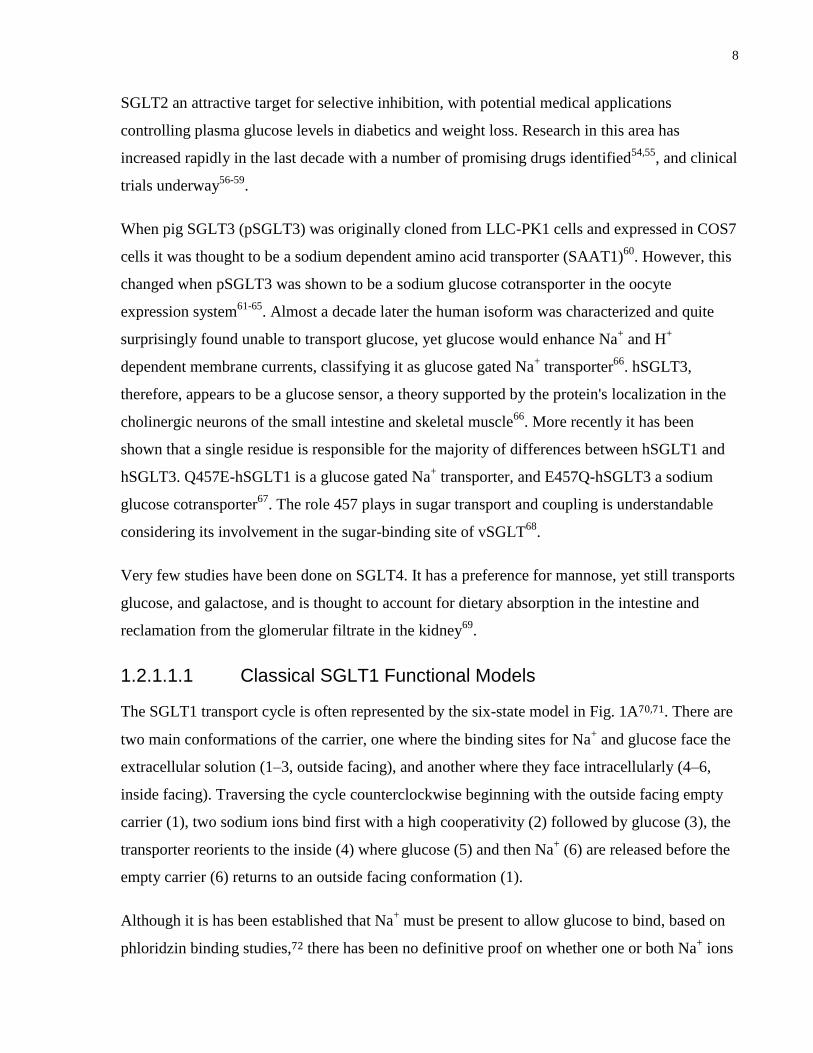
SGLT2 an attractive target for selective inhibition, with potential medical applications
controlling plasma glucose levels in diabetics and weight loss. Research in this area has
increased rapidly in the last decade with a number of promising drugs identified54,55
, and clinical
trials underway56-59
.
When pig SGLT3 (pSGLT3) was originally cloned from LLC-PK1 cells and expressed in COS7
cells it was thought to be a sodium dependent amino acid transporter (SAAT1)60
. However, this
changed when pSGLT3 was shown to be a sodium glucose cotransporter in the oocyte
expression system61-65
. Almost a decade later the human isoform was characterized and quite
surprisingly found unable to transport glucose, yet glucose would enhance Na+ and H
+
dependent membrane currents, classifying it as glucose gated Na+ transporter
66. hSGLT3,
therefore, appears to be a glucose sensor, a theory supported by the protein's localization in the
cholinergic neurons of the small intestine and skeletal muscle66
. More recently it has been
shown that a single residue is responsible for the majority of differences between hSGLT1 and
hSGLT3. Q457E-hSGLT1 is a glucose gated Na+ transporter, and E457Q-hSGLT3 a sodium
glucose cotransporter67
. The role 457 plays in sugar transport and coupling is understandable
considering its involvement in the sugar-binding site of vSGLT68
.
Very few studies have been done on SGLT4. It has a preference for mannose, yet still transports
glucose, and galactose, and is thought to account for dietary absorption in the intestine and
reclamation from the glomerular filtrate in the kidney69
.
1.2.1.1.1 Classical SGLT1 Functional Models
The SGLT1 transport cycle is often represented by the six-state model in Fig. 1A70,71. There are
two main conformations of the carrier, one where the binding sites for Na+ and glucose face the
extracellular solution (1–3, outside facing), and another where they face intracellularly (4–6,
inside facing). Traversing the cycle counterclockwise beginning with the outside facing empty
carrier (1), two sodium ions bind first with a high cooperativity (2) followed by glucose (3), the
transporter reorients to the inside (4) where glucose (5) and then Na+ (6) are released before the
empty carrier (6) returns to an outside facing conformation (1).
Although it is has been established that Na+ must be present to allow glucose to bind, based on
phloridzin binding studies,72 there has been no definitive proof on whether one or both Na+ ions

9
bind before glucose. There have been a few studies which have attempted to distinguish
between the Na+/glucose/Na
+ and Na
+/Na
+/glucose binding orders but they have been
inconclusive, with some suggesting the former73-75 and others the latter76. Regardless, for some
time now the Na+/Na
+/glucose binding order has been the prevalent scheme12,71,77.
In the absence of glucose there is a Na+-dependent phloridzin-sensitive steady-state current
observable in oocytes, which was originally presumed to be caused by a Na+-leak pathway
between states 2 and 5, but has more recently been shown to be the result of a cationic leak
pathway (Na+, Li
+, Cs
+, K
+) that is independent of the carrier translocation steps
78. This leak
pathway is much weaker than Na+ coupled glucose transport, generating a current that is only
2.5% of the αMG inducible current42. Transient currents are only observed in the absence of
glucose (2↔1↔6, yellow shading), as glucose promotes an inside facing conformation where
the carrier is electrically silent. Internal binding of Na+ (6→5) is unfavorable under normal
conditions because of the low intracellular Na+ concentration in oocytes (8.5±0.5 mM79) and a
low intracellular Na+ affinity measured with the reverse transport mode (54.3±7.8 mM 80, 12±4
mM81, 6–50 mM82). A weak pathway between 6↔5 is often (although not always19) used to
rationalize a low occupancy of state 5 in the absence of glucose, limiting these transient models
to sates 1, 2 and 670,83,84. In the presence of glucose substrate is translocated across the
membrane and released intracellularly through the pathway 3↔4↔5 (blue shading).
The demonstration by Chen et al. of two transient decays in the absence of Na+, and our
supporting finding of three in the presence of Na+, necessitates the existence of an intermediate
state of the empty carrier (Fig. 1B, state 7)85,86; there must be at least one transition per decay.
This same reasoning was used to extend the model again when Loo et al. observed three decays
in the absence of Na+ (Fig. 1B, state 8)84.
1.2.1.2 Myo-inositol: SMIT1 and SMIT2
The SLC5 family contains two myo-inositol transporters, SMIT1 (SLC5A3)87
and SMIT2
(SLC5A11)88,89
. Inositol is an important compound in a number of physiological processes, as
an osmolyte90
and a precursor of the inositol phosphate group of secondary messengers91
.
Supplements of inositol have been shown to be effective in treating depression92
, panic
disorder93
, obsessive-compulsive disorder94
, and insulin resistance due to polycystic ovary
syndrome95
.

10
Both transporters have a similar expression profile that includes brain, neuron, heart, kidney,
skeletal muscle, placenta, pancreas and lung—while SMIT2 is additionally found in liver and
intestine 89,96-99
. SMIT1 knockout mice die soon after birth unless given myo-inositol
supplements, from what appears to be undeveloped peripheral nerves leading to the loss of
brainstem control and respiration100,101
. Furthermore, SMIT1 expression is up regulated in cases
of Down syndrome102
and bipolar disorder103
, and down regulated by lithium and other bipolar
drugs104
.
The Na+:substrate stoichiometry for SMIT1
105,106 and SMIT2
105,106 is 2:1. Both carriers share
similar substrates, including myo-inositol, glucose and xylose, but differ in their affinities for
particular isomers. SMIT2 transports D-chiro-inositol, SMIT1 does not; SMIT1 transports both
the L and D isomers of glucose and xylose, SMIT2 only transports the D isomers. SMIT1 is a
high affinity myo-inositol transporter, 50 μM107
, while SMIT2 is low affinity, 120 μM105
.
1.2.1.3 Monocarboxylates: SMCT1 and SMCT2
Two members of the SLC5 family, SMCT1 (SLC5A8) and SMCT2 (SLC5A12), transport short
chain monocarboxylates such as butyrate and lactate108
. Much like the relationship between
SGLT1 and SGLT2, one is a high affinity transporter of lactate (0.16 mM) with a Na+:substrate
stoichiometry of 2:1 (SMCT1)109-111
, while the other is a low affinity transporter (~40 mM) with
a 1:1 stoichiometry (SMCT2)112-114
. The substrates of these transporters carry a −1 charge,
making SMCT2 the only electroneutral member of the SLC5 family, and the only one that
cannot be studied with the two-electrode voltage-clamp (studies of SGLT2, SGLT5 and CHT
are also difficult because of low expression levels in cultured cells and oocytes115
). The rate of
SMCT1 transport was originally thought to be stimulated by a factor of two in the presence of
saturating Cl−, without Cl
− itself being transported
110. However, a more recent study has
discovered that Cl− does not in fact stimulate transporter current, and that the earlier
interpretation was caused by inhibition of the carrier by the Cl− replacement anion cyclamate
116.
The SLC5A8 gene was originally found in the apical membrane of thyroid cells and thought to
passively transport iodine, leading it to be called the apical iodine transporter (AIT)117
.
However, subsequent groups were unable to observe I− transport, and instead found
monocarboxylates to be better substrates and changed the name to SMCT1109,110
. Both
transporters are expressed in the kidney, intestine, brain, and retina, while SMCT1 is

11
additionally found in the thyroid, colon, and salivary glands, and SMCT2 in skeletal muscle108
.
In the kidney SMCT1 is thought to be the high affinity lactate transporter118
, with silencing of
this gene causing lactaturia119
.
Interest in SMCT1 increased recently when it was identified as a silenced gene in most colon
cancers120,121
, and two of its substrates, butyrate and pyruvate, were found to induce apoptosis in
cancerous cells108,120,122,123
. Butyrate is produced at high concentrations in the colon by the
bacterial fermentation of dietary fiber, and it seems silencing of SMCT1 by these cancer cells is
necessary for their survival.
1.2.1.4 Choline: CHT
One of the more unique members of the SLC5 family is the sodium choline transporter, CHT
(SLC5A7)124,125
. CHT is the only SLC5 member to transport a cationic substrate and is located
exclusively in the presynaptic terminals of cholinergic neurons126
, where it mediates the uptake
of choline for the intracellular production of acetylcholine by choline acetyltransferase
(ChAT)127
. The Na+:substrate stoichiometry increases from 2:1 to 9:1 as the membrane potential
is hyperpolarized. Cl− is required to initiate transport but is itself not transported and can be
partially replaced by Br− 124,128
.
CHT has the largest Na+-leak of the SLC5 family at ~40% of the transport current, which may
explain the large Na+ stoichiometry at hyperpolarizing potentials. A remarkably low level of
surface expression complicates the study of CHT in heterologous expression systems. Choline
uptake in CHT expressing oocytes is only 3–4 times greater than background (compared with
1000 times for SGLT19) with maximal choline induced currents of ~13 nA. However, resealed
membrane vesicles made from transiently transfected COS7 cells show significantly more
activity, implying a large intracellular pool129
. A L530A/V531A double mutant appears to
increase trafficking to the membrane by ~2.5 times and permits some electrophysiological
measurements in oocytes124
.
1.2.1.5 Iodide: NIS
The sodium iodide symporter, NIS (SLC5A5)130
, is the primary transporter of iodine into
thyroid cells, but is also found in several other tissues including salivary gland, stomach and
lactating mammary gland131
. Because of this, it plays an important role in delivering radioactive

12
iodine for the treatment of thyroid cancer, and has been proposed as a treatment for some breast
cancers that express NIS132
. NIS has been well characterized in the Xenopus oocyte expression
system where it has been shown to transport Na+:I
− with a 2:1 ratio
133. A single amino acid
mutation (T354P) has been identified as the cause of hypothyroidism in several patients134
.
1.2.1.6 Multivitamin: SMVT
The sodium multivitamin transporter, SMVT (SLC5A6)135
, is expressed most in placenta136
, is
the primary multivitamin transporter in the intestine and liver137
, and can also be found in the
pancreas, kidney and heart. It is known to transport pantothenate, lipoate and biotin with a
stoichiometry of two Na+ per substrate, but all together there are very few kinetic studies of the
transporter135,136
.
1.2.1.7 Orphan: SGLT5
Only a handful of studies have been done on SGLT5 (SLC5A10), which is an orphan transporter
found mostly in rabbit138
and bovine kidney139
, and chicken intestine140
.
1.2.2 The Solute:Sodium Symporter Family
Several non-human transporters that share homology with the SLC5 family are members of the
SSS family, TC 2.A.21. A relatively small number have been characterized, and they are listed
in Table 1. vSGLT from Vibrio parahaemolyticus is the most significant member, because of its
recently solved crystal structure68
, and is a close cousin to SGLT1 transporting Na+ and
galactose with a 1:1 stoichiometry141,142
. The Na+ proline transporter PutP, also with a 1:1:
stoichiometry, is essential for the survivability of the infectious bacteria Staphylococcus
aureus36,37,143
, making it a promising drug target144,145
. As well, a homology mapping of the
PutP sequence with that of the crystalized vSGLT structure has confirmed that they share
similar structures146
. There are only a few studies on the sodium pantothenate transporter
PanF147,148
.
1.2.3 Phylogenetic Homology
An unrooted phylogenic tree of the 12 SLC5 members, 10 SGLT1 species homologs, and three
prokaryotic members of the SSS family is shown in Fig. 2A. All of the SLC5 members that bind
neutral substrates (glucose, inositol, and mannose) are clustered on one branch of the tree

13
(bottom), while anionic binding carriers (monocarboxylates, multivitamin, and iodide) form
another (top left). The only cationic transporter (choline) and the three prokaryotic transporters
are relatively distinct from each other and the other carriers (top). Therefore, with the human
genes the transporters are clearly grouped according to the charge carried by the substrate.
The sequence similarities and identities are shown in Fig. 2B. Amongst the sugar transporters,
SGLT3, a glucose sensor, is most similar to SGLT1, followed by the low-affinity glucose
transporter SGLT2, the mannose transporter SGLT4 and the orphan transporter SGLT5, and the
two myo-inositol transporters SMIT1 and SMIT2. All of the SGLT1 species homologs but
Atlantic salmon are more related to human SGLT1 than any of the other SLC5 members.
1.2.4 Structural Homology
Crystal structures of bacterial secondary active membrane transporters began appearing in 2002
with the oxalate formate exchanger OxlT30
of the major facilitator superfamily (MFS), and the
proton driven multidrug efflux transporter AcrB149
of the resistance nodulation-cell division
(RND) superfamily. Since then, 16 different proteins have been solved and six architectures
have been identified as shown in Fig. 3. A common feature of most of these architectures is a
two-fold axis of symmetry between N and C-terminal 4–6 helix bundles. Evolutionary clues
about the origin of this architectural symmetry have come from the multidrug transporter EmrE
of E. coli, a four-transmembrane homodimer that has also been crystalize150
. It suggests an
evolutionary path where a single gene encoding a dual topology homodimer like EmrE may
undergo a gene duplication event and become an inverse-topology heterodimer, these two genes
can later fuse to encode a monomer with inverted repeats151,152
.
The LeuT fold (the first protein to be crystalized from this family) is the most genetically
diverse, having been found in 7 transporters (LeuT153
, vSGLT68
, Mhp1154
, BetP155
, AdiC156,157
,
ApcT158
, CaiT159
) belonging to 5 phylogenetically distinct families (neurotransmitter:sodium
symporter NSS; solute:sodium symporter SSS; nucleobase:cation symporter-1 NCS1;
betaine/carnitine/choline transporter BCCT; amino acid-polyamine-organocation APC). Each of
these transporter families forms a separate branch in Fig. 3, highlighting their genetic diversity.
Their basic structure is a 5 helix repeat, which is discussed in more detail in §1.3 Crystal
Structures of the LeuT Fold.

14
Other secondary active transporter architectures include the 6 helix repeat MFS transporters
(OxlT30
, eLacY24
, GlpT31
, EmrD32
), the 6 helix repeat RND transporters (AcrB149
, MexB160
), the
unique and intricate 6 helix repeat of the NhaA transporter161
, the unique 8 helix structure with
minor symmetry of the homotrimer dicarboxylate/amino acid:cation symporter (DAACS)
GltPh162
, and the 4 helix homodimer small multidrug resistance (SMR) transporter EmrE150
.
The existence of shared architectures that transcend substantial differences in primary structure
reveals familial relationships at the tertiary level. This is an important finding, because it
suggests the likelihood of shared mechanisms adopted by a wide range of proteins, and as the
field becomes more interconnected the applications of each new discovery are amplified.

15
1.2.5 Figures
Table 1: Properties of SLC5 and select TC 2.A.21 members115
.

16
Fig. 1: Classical SGLT1 transport model. (A) The transport of Na+ and glucose follows an
ordered process; 1 outside facing empty carrier, 1→2 two Na+ bind simultaneously with a high
cooperativity, 2→3 glucose binds, 3→4 fully loaded carrier orients to the inside, 4→5 glucose
unbinds, 5→6 both Na+ unbind simultaneously, 6→1 inside facing empty carrier orients back to
the outside. In the absence of glucose the transient model is restricted to 2↔1↔6 (yellow
shading). The full transport pathway involves 3↔4↔5 (blue). The transporter cycles in an
anticlockwise direction at hyperpolarizing potentials and in a clockwise direction at
depolarizing. (B) Extensions to the classical model, spurred by the discovery of additional
transient decays. An intermediate state of the empty carrier (7) was first discovered by Chen et
al.85 and further supported by Krofchick and Silverman86, while a second intermediate state (8)
was established later by Loo et al.84.

17
Fig. 2: Homology of the SLC5 and SSS families. (A) Phylogenetic tree including SGLT1
species homologues (grey). (B) Sequence similarity and identity shared between SLC5 and SSS
members. Species abbreviation: human, pig, rabbit, rat, Atlantic salmon, mouse, bovine, dog,
sheep, Eurasian common shrew, horse, Escherichia coli, Vibrio parahaemolyticus.

18
Fig. 3: Phylogenic tree of secondary active transport families with solved crystal structures
(stars). See Fig. 2 for species abbreviations.
hSGLT
1hS
GLT3hSG
LT2
hSGLT4hSGLT5
hSMIT2
vSGLT
hSMIT1
hNIS
hSMCT1
hSMCT2
hSMVT
ePutP
ePanFhC
HT
AdiC
Cad
B
PotE
Cad
C
ApcT
SteT
xC
T
CAT
1
NK
CC
2N
CC
GltP
h
LeuT
Aa
hGlyT
1b
hGAT1
hDAT
hSERT
Mhp1HyuP
PUCI
DAL4
FUI1
BetPO
puDButA
BetTEctPCaiTN
haA
MexB
AcrB
eLac
Y
hG
LU
T1
HM
IT
Glp
TEmrD
Oxl
T
0.027
SSS/
SLC
5
APCN
SS/SLC6
NC
S1
BCCT
MFS/SLC2
DAACS
NhaARND
★
★
★
★
★
★
★
★
★★★
★
★
★
★
EmrE
SMR ★
★ crystal

19
1.3 Crystal Structures of the LeuT Fold
The LeuT fold is of particular interest to this thesis because it is shared by a close cousin of
SGLT1, the bacterial Na+/galactose symporter vSGLT of Vibrio parahaemolyticus (Fig. 2B),
and mutation studies have confirmed that vSGLT and SGLT1 have similar structures17,68
.
Understanding the features and conformations of this architecture is essential for developing a
working model that, with the help of kinetic data, may one day explain the mechanisms
involved.
1.3.1 Timeline
The structure of the 2Na+/Cl
−/leucine symporter LeuT of the NSS family was solved in 2005
153.
The core was found to be made out of two symmetrically intertwined bundles, TMs 1–5 and 6–
10, with 11 and 12 trailing on the periphery (see Table 2 for transporter properties and Fig. 4 for
timeline). Over the next few years it was crystalized with a range of amino acid substrates, a
competitive inhibitor163
, and several noncompetitive inhibitors164,165
.
In 2008 another transporter crystal appeared with the same structure, vSGLT68
, but from a
different family (SSS). The 5+5 core was the same, but this time there was one additional TM at
the front and three at the end for a total of 14. Two months later the Na+/benzyl-hydantoin
transporter Mhp1, of the nucleobase:cation symporter (NCS1) family, was solved with the same
TM arrangement as LeuT154
, followed in 2009 by the 2Na+/betaine transporter BetP, of the
betaine/carnitine/choline transporter (BCCT) family, with two extra TMs at the front and one at
the end155
.
At this point it was becoming obvious that transporters with no relation in amino acid sequence
(these were phylogenetically distinct families) or number of TMs (12–14 so far) could share the
same basic architecture, and that other methods of classification might be helpful. With this in
mind, a hydropathy profile alignment of LeuT and vSGLT was used to identify a similar fold for
the amino-acid-polyamine-organocation (APC) superfamily166
, and within a year this hypothesis
was confirmed for two members; the arginine:agmatine antiporter AdiC156,157
and the H+/amino-
acid symporter ApcT158,167
.

20
1.3.2 Architecture
A distinctive feature of the LeuT fold is an internal symmetry relating the first five and last five
TMs of a ten-helix bundle. These 5 TM halves are interwoven to form the carrier, and,
depending on the variant, can be flanked by an additional 2–4 TMs of questionable significance
(Table 2). To keep the notation simple we will adopt the numbering of Abramson and Wright
for the rest of this discussion168
: extra N-terminal helices ( −2, −1), core (1–10), extra C-
terminal helices (11, 12, 13).
As Fig. 5 shows, TMs 1–5 and 6–10 are twisted together to form structural and functional pairs
(1/6, 2/7, 3/8, 4/9 and 5/10) that are related by a two-fold axis of symmetry. Two central pairs,
1/6 and 3/8, make up the core of the transporter by defining the majority of the pore surface, and
substrate and cation binding sites. A unique and important feature are unwound regions at the
midpoint of TMs 1 and 6 that participate in substrate and ion binding, and conformational
changes. Typically one end of the substrate binds at the unwound regions, and the other extends
towards TMs 3/8 (Fig. 5, orange triangle). In some cases (BetP and vSGLT) TMs 1/6 are
wedged apart by the substrate and 2/7 become involved in binding, and in others (AdiC and
vSGLT) 10 bends over the pore to interact as well. Ion binding occurs mostly between TMs 1
and 8, but there is another site between 1, 6 and 7 in LeuT.
The outer shell is made up of TMs 2/7 on one side and two opposing V’s formed by 4-5 and 9-
10 on the other. These V’s pinch the long diagonal 3/8 pair on both ends, while 5/10 support 1/6
from the side, and 2/7 buttress them from behind.
1.3.3 Solved Conformations
The structures captured so far have been found in a variety of conformations, and with various
substrates (Fig. 4). Comparing them provides clues about the mobility of TMs, possible
conformations, and conformational changes, but it is important to keep in mind that there may
be variations in the mechanisms between carriers. For this reason, different conformations of the
same carrier are more valuable, with the ultimate prize remaining one carrier visualized in all
conformations of the transport cycle.
All of the LeuT structures have been found in an outside facing conformation, characterized by
an extracellular pore leading to the binding site, at the unwound regions of TMs 1 and 6, and

21
covered by a thin gate. The first structure was determined with bound leucine153
, with later
structures showing alanine, glycine, leucine, methionine, 4-F-phenylalanine and tryptophan at
the same site163
. Based on these structures, and kinetic data, tryptophan’s mechanism of
competitive inhibition was explained. Other structures with bound tricyclic antidepressants
(TCA) desipramine, imipramine, and clomipramine uncovered the mechanism of
noncompetitive inhibition164,165
.
Mhp1154
and AdiC156,157,167
were also found in an outside facing conformation similar to LeuT,
and were able to be crystalized with and without substrate. These structures have provided
important clues about the conformational changes that take place after substrate binding, and the
gating mechanism.
The existence of an intracellular pore was confirmed with the vSGLT1 structure, which was
found in an inside facing conformation with bound substrate, blocked from release by a thin
intracellular gate68
. ApcT was also crystallized in an inside facing conformation, but without
substrate and the intracellular pore partly occluded158
. The BetP structure is unique, existing in
an intermediate conformation with bound substrate and partially closed pores on either side155
.
1.3.4 Pores
The substrate binding site is located midway across the membrane, at the unwound regions of
TMs 1 and 6, and, depending on the conformation, is accessed by an intra or extracellular
solvent accessible pore. When one pore is open the other is closed by a thick layer of collapsed
TMs, and, in the process of switching, the carrier appears to pass through an intermediate state
where both pores are closed (BetP, ApcT).
As shown in Fig. 6A with LeuT, but also observed for Mhp1 and AdiC, the extracellular pore is
visible between TMs 1, 3, 6, 8 and 10. TMs 1 and 6 bend in unison at their breaks away from
the opening, and along with 3 and 10 line the exit with 8 filling the rear. The extracellular pore
is closed by the inward bending of the tip of TM 10, and the extracellular halves of 1and 6 (see
B and C). This change may occur in two steps, first with the bending of TM 10 seen with Mhp1,
followed by the tilting of 1 and 6 observed with BetP and vSGLT.
vSGLT shows the intracellular pore (C), which is formed by TMs 1, 2, 3, 6, 8 and 10. Again
TMs 1 and 6 bend away, highlighting the flexibility of their unwound centers to allow rotations

22
on both sides. TMs 1, 6 and 8 form the exit, while 2, 3 and 10 line the rear. Tracing the transport
path through these pores sees the substrate enter between TMs 6 and 10 and exit in an S-shaped
motion through 1 and 5.
An intermediate conformation, with both pores closed, is seen in BetP and ApcT (B). In both
cases the cytoplasmic pore is partly open, although not enough to allow the release of substrate.
The presence of three distinct conformations, open-to-out, occluded, and open-to-in suggests
two large scale conformational changes during transport.
1.3.5 Thin Gates
Some of the structures with bound substrate have a fully open pore (LeuT, vSGLT, and AdiC)
yet the release of substrate is prevented by one or more gates, often consisting of the large
aromatic residues phenylalanine, tryptophan and tyrosine. In all three cases the gate residues lie
directly on top of the substrate, locking it in the binding site (Fig. 7A–C).
In the LeuT structure (A) a tyrosine on TM 3 (Y108) and a phenylalanine on TM 6 (F253) pin
the substrate down, with the gates held in place by a salt bridge (R30/ D404) linking TMs 2 and
10 at the mouth of the pore. A single tyrosine on TM 6 (Y263) stacks with galactose in vSGLT
(B), preventing its release to the cytoplasm, a feature commonly shared by sugar binding
proteins24,169
. Although the extracellular pore is closed for vSGLT, three gates lay directly on
top of the galactose (M73, Y87, and F424) which bonds with the OH group of Y87. Three layers
of gates have been proposed for the AdiC structure (C). A middle gate (W293) separates distinct
intracellular and extracellular binding sites that are enclosed by their own intracellular (Y93,
E208, and Y365) and extracellular (W202 and S26) gates. This unique gate structure is thought
to be necessary to accommodate the antiporter nature of AdiC. Arginine would be transported
intracellularly by first passing through the extracellular and then intracellular binding sites, and
once in an inward facing conformation agmatine would be transported out by passing through
the two binding sites in reverse order. This mechanism would allow the extracellular binding
site to have a higher affinity for arginine, and the intracellular binding site a higher affinity for
agmatine. How far might a gate travel between open and closed conformations? Comparing
AdiC structures with and without arginine shows a tryptophan gate on TM 6 (W202) travelling
10 Å to reach the closed conformation, caused by a 40° rotation of TM 6 around the unwound
region167
.
23
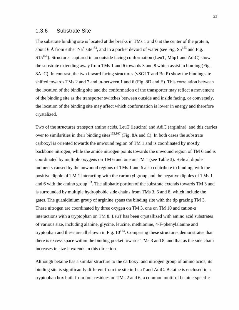
1.3.6 Substrate Site
The substrate binding site is located at the breaks in TMs 1 and 6 at the center of the protein,
about 6 Å from either Na+ site
153, and in a pocket devoid of water (see Fig. S5
153 and Fig.
S15158
). Structures captured in an outside facing conformation (LeuT, Mhp1 and AdiC) show
the substrate extending away from TMs 1 and 6 towards 3 and 8 which assist in binding (Fig.
8A–C). In contrast, the two inward facing structures (vSGLT and BetP) show the binding site
shifted towards TMs 2 and 7 and in-between 1 and 6 (Fig. 8D and E). This correlation between
the location of the binding site and the conformation of the transporter may reflect a movement
of the binding site as the transporter switches between outside and inside facing, or conversely,
the location of the binding site may affect which conformation is lower in energy and therefore
crystalized.
Two of the structures transport amino acids, LeuT (leucine) and AdiC (arginine), and this carries
over to similarities in their binding sites153,167
(Fig. 8A and C). In both cases the substrate
carboxyl is oriented towards the unwound region of TM 1 and is coordinated by mostly
backbone nitrogen, while the amide nitrogen points towards the unwound region of TM 6 and is
coordinated by multiple oxygens on TM 6 and one on TM 1 (see Table 3). Helical dipole
moments caused by the unwound regions of TMs 1 and 6 also contribute to binding, with the
positive dipole of TM 1 interacting with the carboxyl group and the negative dipoles of TMs 1
and 6 with the amino group153
. The aliphatic portion of the substrate extends towards TM 3 and
is surrounded by multiple hydrophobic side chains from TMs 3, 6 and 8, which include the
gates. The guanidinium group of arginine spans the binding site with the tip grazing TM 3.
These nitrogen are coordinated by three oxygen on TM 3, one on TM 10 and cation-π
interactions with a tryptophan on TM 8. LeuT has been crystallized with amino acid substrates
of various size, including alanine, glycine, leucine, methionine, 4-F-phenylalanine and
tryptophan and these are all shown in Fig. 10163
. Comparing these structures demonstrates that
there is excess space within the binding pocket towards TMs 3 and 8, and that as the side chain
increases in size it extends in this direction.
Although betaine has a similar structure to the carboxyl and nitrogen group of amino acids, its
binding site is significantly different from the site in LeuT and AdiC. Betaine is enclosed in a
tryptophan box built from four residues on TMs 2 and 6, a common motif of betaine-specific

24
binding proteins required to prevent the repulsion of this highly hydrophilic osmolyte by the
protein backbone155
(Fig. 8D). This tryptophan box is one section of a hydrophobic pathway
spanning the membrane (Fig. 7E). It has been proposed that betaine travels through several of
these binding sites during transport.
Galactose is bound in vSGLT by a perimeter of two charged and four polar residues that
hydrogen bond with the six substrate oxygen through two backbone oxygen, two side chain
oxygen, and four side chain nitrogen situated on TMs 1, 2, 6, 7 and 10 (Fig. 8E and Table 3).
The galactose is then sandwiched on both sides by one intracellular and three extracellular
hydrophobic gates (Fig. 7B).
In the Mhp1 structure benzyl-hydantoin is folded into a V-shape with the tip pointing
intracellularly (Fig. 8B). The hydantoin and benzene rings form pi-stacking interactions with a
tryptophan on TM 3 and 6, and the remaining oxygen and nitrogen atoms bond with four polar
residues on TMs 1, 3 and 8.
1.3.7 Cation Sites
Given the similar architectures of the LeuT fold structures, there are a surprising variety of
cations that can be accommodated. Two of the six structures are Na+ symporters, transporting
one Na+ ion (Mhp1 and vSGLT), two transport two Na
+ ions (LeuT and BetP), one is a virtual
proton antiporter (AdiC) and another a proton symporter (ApcT) (Table 2). This diversity
appears to be accomplished through a shared cation binding site between all of the structures (no
site was found for AdiC). This site, referred to as Na2 based on its naming in the LeuT structure,
is located between TM 8 and the unwound region of TM 1 half way across the membrane (Fig.
9). Coordination of Na+ at the Na2 site is remarkably similar for all of the transporters (Table 3).
It involves five oxygen, 60% backbone from hydrophobic residues (Ala, Ile, Met, Val and Gly)
of which 50% are alanine, and 40% side chain oxygen of polar residues (Ser and Thr). The bend
in TM 1 contributes two backbone oxygen, with one backbone and two side chain oxygen
coming from TM 8 (TM 5 is also involved in BetP). This corresponds to a trigonal bipyramid
arrangement in LeuT153
and a square pyramid in Mhp1154
. Cation coordination at the Na2 site of
ApcT is unique because it involves the binding of a proton, instead of Na+, to a lysine residue
protruding from TM 5 into the Na2 site. This protonated lysine is then coordinated by one
backbone oxygen on TM 1 and one side chain oxygen on TM 8.

25
Two of the crystallized transporters, LeuT and BetP, operate with a 2:1 cation:substrate
stoichiometry. As expected, a second Na+ site, Na1, adjacent to Na2 and the ligand carboxyl
group has been identified for both. Na1 is located between TMs 1 and 7 in LeuT and between
TMs 1, 3, 6 and 8 in BetP (Fig. 9D and E, and Fig. 5). In both cases, multiple backbone and side
chain oxygen are involved as well as the substrate carboxyl group (Table 3). In the LeuT
structure these coordinating oxygen are arranged in an octahedral. Participation of the substrate
carboxyl in Na+ binding demonstrates the potential for direct coupling between the substrate and
ligand.
LeuT is the only protein with the LeuT fold that interacts with a chloride ion, and is also the
only structure containing an extracellular helix between TMs 3 and 4, adjacent to the chloride
(Fig. 5). This extracellular helix, along with TMs 4 and 8, form the Cl− binding site. However, it
is not immediately clear how Cl− affects the transporter from this position at the periphery.
1.3.8 Inhibitor Sites
LeuT is currently the only transporter with the LeuT fold that has been crystallized in the
presence of inhibitors. However, because of the simplicity of these mechanisms there is a good
chance that the other structures are inhibited in a similar way.
A number of amino acids of various sizes are transported by LeuT including glycine, alanine,
leucine, methionine and tyrosine. However, tryptophan is not, and instead acts as a competitive
inhibitor, becoming wedged in the binding cavity because of its large indole ring (Fig. 10F). The
extracellular gates, Y108 and F253, are forced apart 3 Å by tryptophan (Fig. 11A, and compare
Fig. 10F and E), and the R30/D404 salt bridge is separated by 8 Å, preventing its formation and
allowing solvent access to the binding site163
. In this state the extracellular pore cannot close,
nor can the transporter progress to an inside facing conformation, thus preventing intracellular
release. Three additional low-affinity binding sites were also identified (Fig. 11B). One is
located in the extracellular pore between R30 and D404, and blocks the extracellular release of
tryptophan at the high affinity site. There are also two other sites on the periphery, but they are
not thought to be in functionally significant areas163
.
LeuT belongs to the neurotransmitter sodium symporter (NSS) family, which is inhibited non-
competitively by tricyclic antidepressants (TCA). TCAs were commonly used to treat

26
depression, presumably through an interaction with NSS members, but have been replaced in
recent years by selective serotonin reuptake inhibitors (SSRI), which are considered to have
more favorable side effects. The mechanism of TCA inhibition is elucidated by the LeuT
structures bound with leucine and the TCAs clomipramine, imipramine and desipramine. In all
cases the TCAs bind directly above the extracellular gates, Y108 and F235, and occupy the
extracellular pore164,165
(Fig. 11C). The TCAs reinforce the salt bridge between R30 and D404
by bringing the residues closer together, and the bulky TCA shields the salt pair from solvent. In
addition, R30 is held firmly in place by a cation-π interaction with the extracellular gate F253
directly below, the TCA directly above, and a hydrogen bond network between its guanidine
group, the sodium at the Na1 site, and the substrate’s carboxyl164
. Lastly, a salt bridge between
the TCA’s N2 atom and D404 anchors the inhibitor (Fig. 11C). These interactions work together
to stabilize the TCA within the extracellular pore, and outline the mechanism of non-
competitive inhibition. An additional low affinity TCA binding site is located at the intracellular
tip of TMs 4–5, but it is not clear if this site is functionally significant (Fig. 11D).
Competitive inhibition is possible when the substrate has the key carboxyl and amide motif
common to amino acids, but a side chain that is too bulky to fit within the binding pocket.
However, as illustrated by tryptophan binding to LeuT, a secondary binding site within the
extracellular pore (alternate site 1) may be required to prevent the inhibitor’s release (Fig. 11B).
It is possible that the other cotransporter structures are inhibited in similar ways, as may be the
case for phloridzin inhibition of SGLT1, considering that phloridzin is the natural substrate
glucose bonded at the C1 position to phloretin. However, there is some evidence that phloridzin
is transported, in which case the inhibition mechanism may be a very slow translocation
step170,171
. In comparison, non-competitive inhibition involves binding within the extracellular
pore, and stabilization of the protein conformation, possibly through a salt bridge interaction.
1.3.9 Thick Gates
Not all of the structures retain the substrate with a thin gate layer. Mhp1 holds the substrate in
the extracellular binding pocket by bending TM 10 over the pore, essentially using the helix as a
gate (Fig. 7D). BetP and ApcT were crystallized in an intermediate conformation with both
pores partially closed to various degrees by the collapsing of the surrounding TMs (Fig. 7E and
F). In the BetP structure there is a rather long pathway spanning the membrane between TMs 1,

27
2, 6 and 7, lined by 23 highly conserved aromatic residues in BetP and the
betaine/choline/carnitine transporter (BCCT) family155
. It has been proposed that this
hydrophobic pathway allows the hydrophilic osmolyte betaine to travel through the protein
without being repelled by the protein backbone. In the crystal structure betaine is trapped within
a four residue tryptophan box, but is thought to travel through multiple binding sites of this type
that line the pathway and are potentially separated by a series of gates155
. There is no substrate
bound in the closed ApcT structure but both pores are blocked by inward bending TMs.
There appear to be two complementary mechanisms for occluding the binding sites of these
carriers. Thin gates that interact directly with the substrate, often sandwiching it in place and
leaving the pore intact (LeuT, vSGLT, and AdiC), and thick gates that involve occlusion of the
pore by multiple collapsed TMs (Mhp1, BetP, and ApcT). There is also variation in the extent of
thick gate collapse between an initial lightly closed state (Fig. 7D–F), and a tightly packed one
formed when the carrier orients to the other side (Fig. 6A and C).
1.3.10 Conformational Changes
The Mhp1 and AdiC structures were solved with and without substrate. In both cases
conformational changes take place after binding that result in partial closing of the extracellular
pore. In the case of Mhp1 the extracellular tip of TM 10 bends substantially at its midpoint
towards the pore and traps the substrate154
. This motion is enabled by an adjacent glycine and
proline at positions 371 and 372. Mhp1 is the only transporter seen in an outside facing
conformation with this bend in TM 10. However vSGLT and BetP whose structures have been
solved in inside facing states both show this bend, which occurs at G432 in vSGLT and P528 in
BetP (see Fig. 6B and C).
After substrate binding to AdiC there is a large movement of the extracellular half of TM 6, and
smaller movements in TMs 2 and 10, towards the pore (see Fig. S8167
). TM 6 rotates 40° about
its unwound region, moving W202 10 Å to interact with the aliphatic portion of the substrate.
Considering that a residue on TM 6 moves to make contact with the substrate in both Mhp1 and
AdiC, it is possible that the substrate pulls on TM 6 causing the motion. All of the LeuT fold
structures make contact on TM 6 with the substrate and therefore this mechanism may be
common to all of the transporters.

28
Other conformational changes can be deduced by comparing different transporters in different
conformations. TMs 1 and 6 seem to play a major role in allowing access to both the intra- and
extra-cellular pores. Each half of these split TMs seem to move independently to block or
expose each pore with the unwound region acting as a hinge (see Fig. S14172
). Outside facing
structures (LeuT, Mhp1 and AdiC) have the extracellular half of TMs 1 and 6 bending away
from the extracellular pore allowing access, while the intracellular halves lean in blocking the
inside pore. Intracellular facing structures (vSGLT and ApcT) show an opposite trend. BetP,
which is in an intermediate conformation, has TMs 1 and 6 bending away from both pores,
confirming the potential for each half of TMs 1 and 6 to move independently.
1.3.11 Transport Model
Using the variety of crystal structures as a guide we can put together a sequence of
conformational changes that are likely to take place during the translocation of substrate168,173
.
The proposed model is shown in Fig. 12 and the corresponding crystal states are arranged
below. Mhp1 and AdiC were found in an outside facing state with a clear path to the binding
site (state 1). Thin gates can close and block the binding site (2), but a solvent accessible pore
remains (AdiC and LeuT). The pore is then covered by one or more TMs acting as thick gates
(3), with no clear path on either side of the membrane (Mhp1, ApcT, BetP). The thick
intracellular gates open to reveal the intracellular pore (4), but a thin gate blocks release of the
substrate (vSGLT). The thin gate must then open to release substrate (5), although no structures
have been captured in this state yet. This model suggests that four transitions occur during
transport. Two large scale conformational changes, where whole TMs act as thick gates to
alternately expose pores on either side of the membrane. Two smaller conformational changes,
where thin gates made of several hydrophobic residues move to expose the binding site to either
pore.
This mechanism has been referred to as a gated rocker-switch173
, where the rocker-switch
motion involves the pore switching between inside and outside facing conformations. This is
similar to the rocker-switch mechanism proposed for the major facilitator superfamily, except
without the gates. However, the MFS rocker-switch motion may occur in one step because they
lack the unwound helix structures of TMs 1 and 6 likely required for independent pore
movement.

29
1.3.12 Figures
Table 2: Properties of the LeuT fold transporters.

30
Table 3: Gate, substrate and cation interacting residues for the LeuT fold transporters.
Associated TM segments are colored and labeled, and the interacting O, N or Se is indicated at
the end. Residues with hydrophobic interactions are marked with a ∆, and cation-π with π. Gate
residues are labeled with E (extracellular), M (middle) and I (intracellular) and salt bridge pairs
are labeled ES (extracellular) IS (intracellular).

31
Fig. 4: Timeline of discovery for the LeuT fold structures. Structures are shown in the various
conformations they were obtained, and with transported substrate (green) and/or inhibitor (red). Outside
facing (up), inside facing (down), ions (blue circles), closed gate (black bar), and in some cases a
partially closed pore (small opening). The same structures are sorted by conformation on the bottom.
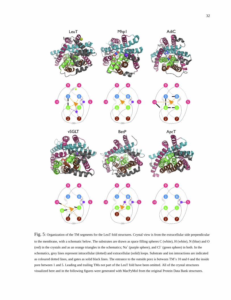
32
Fig. 5: Organization of the TM segments for the LeuT fold structures. Crystal view is from the extracellular side perpendicular
to the membrane, with a schematic below. The substrates are drawn as space filling spheres C (white), H (white), N (blue) and O
(red) in the crystals and as an orange triangles in the schematics; Na+ (purple sphere), and Cl− (green sphere) in both. In the
schematics, grey lines represent intracellular (dotted) and extracellular (solid) loops. Substrate and ion interactions are indicated
as coloured dotted lines, and gates as solid black lines. The entrance to the outside pore is between TM’s 10 and 6 and the inside
pore between 1 and 5. Leading and trailing TMs not part of the LeuT fold have been omitted. All of the crystal structures
visualized here and in the following figures were generated with MacPyMol from the original Protein Data Bank structures.

33
Fig. 6: Extracellular and intracellular pores demonstrated by LeuT, BetP and vSGLT. (A) LeuT,
an extracellular solvent accessible pore is found between TMs 1, 3, 6, 8 and 10, while at the
inside the substrate is occluded by a cluster of TMs. (B) BetP, both pores are partially closed.
(C) vSGLT, the intracellular pore is lined by TMs 1, 2, 3, 6, 8 and 10, while the extracellular
pore is collapsed.

34
Fig. 7: Gating mechanisms. (A) Two gates (Y108 and F253) and a salt bridge (R30/D404) block
the extracellular pore of LeuT. (B) One gate blocks the intracellular pore (Y263), and three line
the extracellular side (M73, Y87, and F424) of vSGLT. (C) Three layers of gates in AdiC, two
at the extracellular side (S26 and W202), one in the middle (W293), and three at the cytoplasm
(Y93, E208, and Y365). (D) TM 10 folds over the binding site locking in the Mhp1 substrate.
(E) A partially closed pathway lined with aromatic residues follows the length of the protein,
suggesting multiple gated binding sites. (F) Inside and outside pores of ApcT partially closed by
the surrounding TMs, in the absence of substrate.

35
Fig. 8: Substrate binding site. The substrate binds between TMs 1, 3, 6 and 8 in LeuT (A), Mhp1 (B) and
AdiC (C), structures captured in an outside facing conformation. In the two inside facing conformations
BetP (D) and vSGLT (E), the substrate is moved away from TMs 3 and 8, towards TMs 2 and 7 behind.
The AdiC and vSGLT structures also show involvement of TM 10. Interacting residues are shown while
TMs not involved in substrate binding are transparent; for residues see Table 3.

36
Fig. 9: Cation binding sites. All of the structures have a common cation binding site at the Na2
position between TM 8 and the bend in TM 1. For vSGLT (A) and Mhp1 (B) this is the only
binding site for Na+, while in ApcT (C) this site is occupied by a proton carried by a lysine on
TM 5. LeuT (D) has an additional Na+ site between TM 7, the bends in TM 1 and 6, and the
substrate carboxyl. For BetP a second Na site has been predicted between TM 8, the bend in
TM1, and the substrate carboxyl; while the Na2 site is assisted by two residues on TM 5.
Substrates are shown as white (carbon), red (oxygen), blue (nitrogen), and purple (Na+) spheres.
Interacting residues are shown (see Table 3).
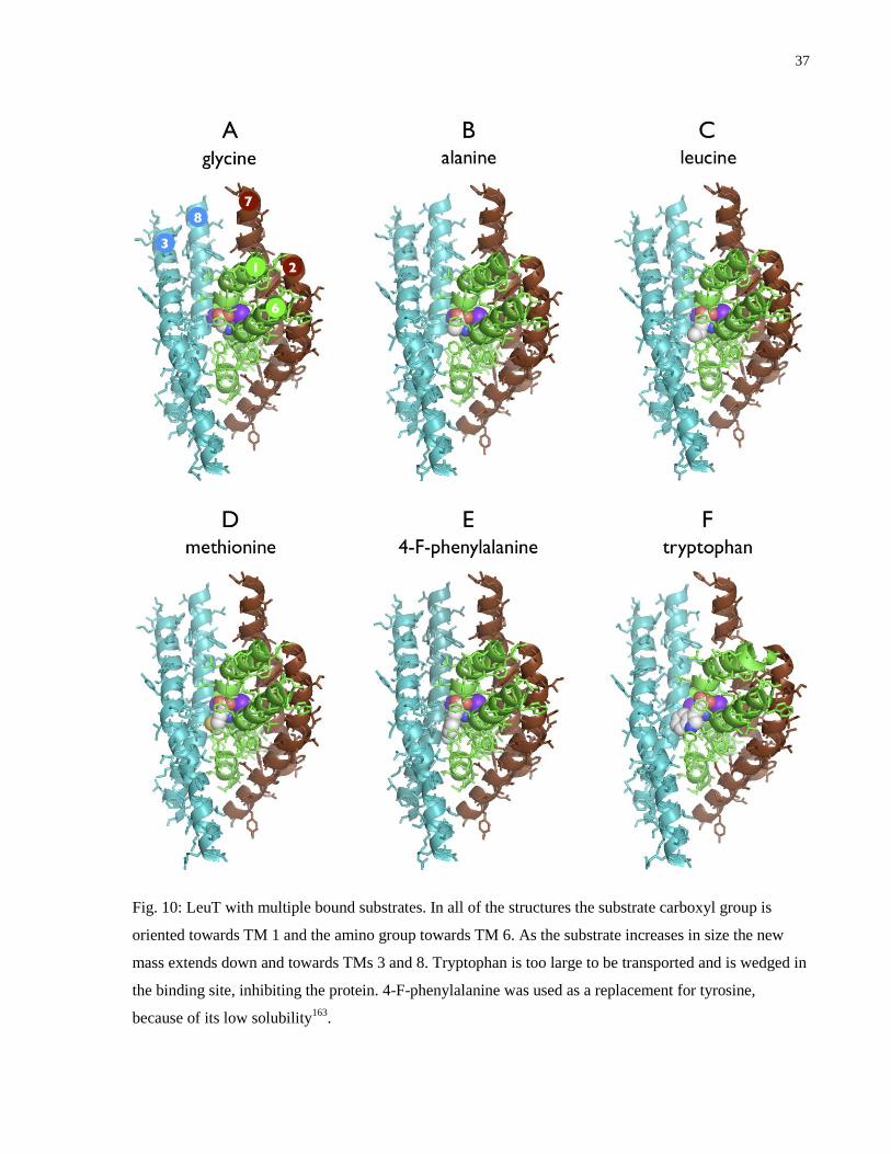
37
Fig. 10: LeuT with multiple bound substrates. In all of the structures the substrate carboxyl group is
oriented towards TM 1 and the amino group towards TM 6. As the substrate increases in size the new
mass extends down and towards TMs 3 and 8. Tryptophan is too large to be transported and is wedged in
the binding site, inhibiting the protein. 4-F-phenylalanine was used as a replacement for tyrosine,
because of its low solubility163
.

38
Fig. 11: Competitive and non-competitive inhibitor binding sites in LeuT. Tryptophan competes for the leucine
binding site in LeuT (A), where it wedges the extracellular gates, Y108 and F253, and salt bridge, R30/D404, open.
There are three alternate tryptophan binding sites (B), located in the extracellular pore (1), the extracellular loop
between TMs 7 and 8 (2) and intracellularly at the base of TMs 1 and 7 (3). Clomipramine is a non-competitive
inhibitor that binds in the extracellular pore between the R30/D404 salt bridge. An alternate clomipramine binding
site is located intracellularly between TMs 4 and 5 (D). Desipramine and imipramine bind to the same high and low
affinity sites as clomipramine. Most intra and extracellular loops have been removed for clarity.

39
Fig. 12: Transport model predicted by the various conformations of the LeuT architecture
captured in crystal structures. The core of the carrier is represented here by the two unwound
helices 1 and 6, which bind substrate at their center and facilitate the rocker-switch motion. Thin
gates (black) composed of several hydrophobic amino acids have been found at the entrances to
the intra and extracellular pores. Thick gates comprised of one or more bent or collapsed TMs
fill the pore on either side, and transition the carrier between inside and outside facing
conformations. Transport begins in state 1 with an open extracellular gate and pore, substrate
binds and the gate closes (2), the outside pore closes leading to an intermediate state (3), the
inside pore opens resulting in an inside facing conformation (4), the inside gate opens and
releases substrate (5). Captured transporter structures associated with each of the model states
are shown below.

40
1.4 Rationale
Electrophysiology has become an important tool in the study of membrane transporter proteins
because it provides superior control over them via the membrane potential, and rapid high-
resolution measurement of transporter activity via the membrane current. It is often the preferred
method of characterization by providing a wide range of kinetic measurements through the
study of transient and steady-state transporter currents. Despite being an excellent experimental
system with access to a variety of kinetic parameters ( , , , , ), there remains a
disconnect between these parameters and an understanding in terms of a model or mechanism.
The goal of this thesis is to find ways to extract as much kinetic information as possible from the
transient and steady-state currents, to achieve a more intimate view of carriers in action, and
come closer to understanding how they work.
All of the experimental work presented in this thesis—the transient kinetic studies of SGLT1 in
§2 Dissecting the Transient Current of SGLT1 and the sampling of steady-state data analyzed in
§3 A Practical Method for Characterizing the Voltage and Substrate Dependence of Membrane
Transporter Steady-State Currents—were collecting with the Xenopus laevis oocyte expression
system using the two-electrode voltage-clamp technique. SGLT1 DNA or RNA is injected into
the oocytes and over a period of 4–6 days transporter protein is grown in abundance and inserted
into the membrane. The large size of these oocytes allows them to accommodate two electrodes,
of which one is used to measure the membrane potential, while the other controls it by injecting
current through a feedback loop to maintain the desired voltage; this injected current is the
current measured during experiments. This system is one of the few ways available for studying
the electrogenic properties of cotransporters because of their small currents and normally small
expression levels in native tissues. The majority of the data presented here is from experiments
with SGLT1 and several SGLT1 mutants, as this carrier has been the primary focus of our lab
for some time. SGLT1, however, is an excellent model system for ion-coupled cotransport in
general, and, therefore, the ideas presented here can be applied to many other ion-coupled
cotransporters and, perhaps, some pumps and cannels. SGLT1 was used to initially demonstrate
the viability of expression cloning in oocytes, and this head start has put it at the forefront of
cotransporter kinetic studies, making it, arguably, the most kinetically well characterized
cotransporter.

41
The current that arises in response to a step-change in membrane potential has two phases. An
initial transient phase, marked by an exponentially decaying current as the carriers settle,
followed by a steady-state, during which the carriers cycle as they transport substrate. Thinking
about the transport model in terms of a sequence of states connected in a loop (e.g. Fig. 1A), the
transient and steady-state currents provide uniquely tinted windows of different regions of this
loop. As will be shown in the two research chapters that follow, the transient current is a family
of exponential decays that directly monitor conformational changes of the protein, while the
steady-state current measures the cycling rate, which is affected by rate limiting segments of the
loop. Transient experiments are typically more difficult to implement and analyze than steady-
state, but the payout in kinetic detail is worth it, as this is the only means to observe individual
transitions of the protein. In contrast, steady-state currents measure lumped parameters, but the
data is easy to collect and analyze, and reveals parts of the loop that are normally inaccessible to
transient studies. Since each type of study exposes different segments of the transport loop in
different ways, both are needed to build a complete a model of the transporter.
Within the past decade significant advancements in the field of membrane protein
crystallography have resulted in the first high resolution structures of channels, pumps, and
cotransporters. While more recently the LeuT architecture has been found throughout a broad
superfamily of Na+ coupled cotransporters, of which SGLT1 is a member. The variety of
conformations that this LeuT architecture has been captured in seems to identify a gated rocker-
switch mechanism that confirms the alternating access hypothesis proposed 45 years ago by
Jardetzky2. Although we are now at the point where we can visualize these structures in great
detail, their dynamics remain a mystery. It is the view of this thesis that by combining these
structures with comparably detailed kinetic data, we can fill in the missing pieces and complete
the picture of how transporters work.
In §2 Dissecting the Transient Current of SGLT1, the transient currents of SGLT1 are
decomposed into as many decay components as possible, to study the conformational changes
they report on and learn about the gated rocker-switch mechanism. This is normally a hard
problem to solve, yet we present a methodology that is successful and can be repeated with
other ion coupled cotransporters. In §3 A Practical Method for Characterizing the Voltage and
Substrate Dependence of Membrane Transporter Steady-State Currents, a general theoretical
model of membrane transport is developed and used to understand the voltage and substrate

42
dependence of the steady-state currents. This ultimately leads to a phenomenological method for
characterizing the classic I–V curves, and an understanding of the parameters that are derived as
representations of rate limit segments of the transport loop. These parameters can then be used
to reconstruct a steady-state model of the carrier. For both the transient and steady-state phases
we have attempted to extract as much kinetic information as possible, and, in each case, this has
resulted in more direct and simple ways of understanding the data in terms of a kinetic model.

43
Dissecting the Transient Current of SGLT1 2
2.1 Introduction
Electrophysiological studies of cotransporters, and in particular their kinetic characterization,
have been common practice ever since expression cloning was demonstrated 25 years ago in the
heterologous Xenopus laevis oocyte system using SGLT1 as a model protein9. This system
provides an opportunity to stimulate overexpressed carrier proteins residing within the cell
membrane by controlling the membrane potential with electrodes. The stimulated carriers
undergo conformational changes that can be studied by monitoring at the membrane current
generated by charged amino acids on the protein or ions as they move, or are isolated, within the
membrane electric field.
This electrophysiological system provides a unique opportunity to observe the transient kinetics
of membrane proteins, generated by step-changes in membrane potential, because of the high
speed with which the membrane potential can be controlled and the carrier currents measured.
These transient currents reflect the kinetics of the overexpressed carriers as they equilibrate
between their initial distribution prior to the voltage jump and the steady-state distribution after
the voltage jump. In 1992, several years after expression cloning was introduced, the first
transient experiments with SGLT1, and one of the first for any cotransporter, were performed174
.
They found that SGLT1 produces transient currents in the absence of glucose, and the addition
of glucose inhibits them. This behavior has been explained recently by showing that glucose
promotes an inside facing conformation where the carrier is electrically silent, hence the absence
of transient current—this corresponds to movement between states 4, 5, and 6 in the classical
model of SGLT1 shown in Fig. 1A77,175
. In the absence of glucose the carrier is restricted to
movement between states 1, 2, and 6, and it is the conformational changes of the empty carrier
1↔6 that are believed to generate current, as Na+ binding is typically much too fast to observe
(0.004176–0.06177 ms). Although state 5 is technically active in the absence of glucose, its
occupancy is highly unfavorable under normal conditions (low intracellular Na+), and is
typically ignored.
44
Recent crystallographic data of a superfamily of cotransporters that share a common architecture
with SGLT1 has provided deeper insights into the conformational changes of the carrier, as
discussed in §1.3 Crystal Structures of the LeuT Fold. As shown in Fig. 12, the various states
that these cotransporters have been crystalized in sketch out a transport mechanism, termed a
gated rocker-switch, that involves four conformational changes of the carrier, situated between
states 1↔6 (and 3↔4) in the classical model of Fig. 1. This mechanism works by mediating
movement in and out of a central substrate binding pocket by way of a mobile pore and gate on
each side of the membrane. One of the few ways of observing these conformational changes in
action is through the transient kinetics. The transient current consists of a number of exponential
decays equal to one less than the number of carrier states, and for a non-cyclical system, like
1↔6, this results in one decay per transition. As we will show, by measuring the decay time
constants (τ) and amplitudes (A) we can learn about the rates and ordering of these transitions.
There are, however, significant challenges involved in the measurement and analysis of these
transient currents. In particular, with respect to the problem of multi-exponential fitting, and the
stimulation of sufficiently large transient currents for accurate fitting.
Multi-exponential fitting is a notoriously difficult task, because of the interconnectedness of the
decays. As will be demonstrated, fitting with an insufficient number of decays skews the results
into a type of weighted average of the true carrier kinetics, and these results can have the
unintended consequence of obscuring the underlying mechanism. However, it can be difficult to
find the correct number of decays, since, at the onset, there is no way of knowing how many to
look for. In addition, it becomes geometrically harder with each exponential term added to the
fit equation to perform the fits and find a successful solution. This project is focused on the
general problem of transient analyses using SGLT1 as a model system; SGLT1 was one of the
first cotransporters to be studied using these techniques, and has become one of the most well
characterized kinetically. A unique protocol is presented for collecting transient data that uses
multiple holding potentials to produce large decays. Also, a methodology for multi-exponential
fitting is demonstrated that provides measures for evaluating the quality of a fit and indicators
for helping to decide when too few or too many exponential terms are being used.
As discussed in the next section initial transient studies of SGLT1 characterized the transient
currents with a single exponential decay, but over time this number has gradually increased to
three. However, the current model based on the crystallographic data suggests four

45
conformational changes of the carrier, and therefore four decays. In this study the transient
kinetics of SGLT1 and a threonine to cysteine mutant at position 156 (T156C) were
characterized using these new methods. Four carrier decays were found for each, in agreement
with the crystallographic model, with rates of 2, 5, 25, and 50–200 ms. In addition, charge
movements for each decay (Q=Aτ) were found to differ depending on the direction of the
voltage jump. This phenomena suggested that some transitions might be masked when moving
in one direction, and this was interpreted as an effect seen when a slow transition is in front of a
faster one and hides it. Using this directional charge information, four conformational changes
were aligned in series in a way that could explain the data. When this kinetic model was then
aligned with the crystallographic, the fast decays (2 and 5 ms) were found to correspond with
movement of the intra and extracellular gates, and the slow decays (25 and 50–200 ms) with the
intra and extracellular pores. Although these experiments were performed with SGLT1, the
techniques presented here are general enough to be used on a wide variety of electrogenic
cotransporters that produce transient currents. Furthermore, now that the gated rocker-switch
mechanism has been described kinetically, other carriers can be tested for a similar or different
mechanism.
2.1.1 The T156C Mutant
We decided to study the T156C mutant because it is located in a critical region for substrate
binding. This is exemplified by the neighboring lysine to cysteine mutation K157C, which
completely abolishes glucose and phloridzin binding16. It is our hypothesis that access to the
binding site is blocked, and that the lysine at this position is possibly involved in a salt bridge
that mediates a conformational change that provides access to the binding site. The T156C
mutant retains full function, making it more suitable than K157C for kinetic studies, but has a
significantly reduced apparent affinity for the inhibitor phloridzin (30–170 μM versus 1.6±0.6
µM for wt, Fig. 13A). This reduced affinity alters the interaction of phloridzin with the carrier
into a weak inhibitor that unbinds when the membrane potential is depolarized. This behavior
can be observed as a new slow decay that appears in the presence of phloridzin (Fig. 13C), and
stands out from phloridzin`s normal role as a tight-binding inhibitor178. Lastly, the Q–V
distribution, measured by integrating the transient charge movements, is right-shifted by a large
amount (38 mV, Fig. 13B), indicating that the carrier has difficulty changing into an inside-
facing conformation (i.e. with the extracellular pore closed and the intracellular open). These
46
characteristics appeared to indicate an affected conformational change, making this mutant an
interesting candidate for transient studies. As shown in Fig. 14, by the placement of their aligned
residues in the vSGLT structure T156 and K157 are near, and equidistant to, the Na+ and
glucose binding sites. This places them in an active region of the carrier that is consistent with
effect of their mutations.
2.1.2 Historical Perspective
The first electrogenic study of SGLT1 transient kinetics was performed in 1992 on the rabbit
isoform, by observing conformational changes of the empty carrier in the absence of
glucose70,174. The transient decays were fit with a double exponential and steady-state term
( ⁄ ⁄ ), finding a fast (0.95–2.3 ms) and slow (4–18 ms) component.
Despite some voltage dependence the fast was concluded to be voltage independent and was
assigned to the membrane capacitance (typically ~0.5 ms), while the slow peaked at negative
potentials, was sensitive to αMG and phloridzin, and was attributed to the carrier. These
observations were repeated the following year for the human carrier (fast 0.54–0.82 ms, slow 2–
8 ms), with the fast again being assigned to the membrane, and the slow peaking, instead, at
positive potentials83. Attempting to find the amino acids responsible for the difference between
the slow decay of rabbit and human, the D176A mutant of rabbit was characterized in 1994179.
In this case, the fast decay was too slow (2.5–4.6 ms) to attribute to the membrane capacitance,
yet this was overlooked despite hinting at the presence of a second carrier decay. The slow time
constant peak did shift to positive potentials (4.6–28 ms) to resemble human, but there were
other factors that led to the conclusion that other amino acids were responsible for the
differences between species.
With these early studies two protocols were commonly used to analyze the transient currents of
SGLT1 and other carriers, and in particular in how they dealt with the membrane capacitance.
The subtraction method involved subtracting readings with and without an inhibitor to remove
the membrane and endogenous currents, and isolate the carrier current which was then fit with a
single exponential (SGLT183, GAT1180, SERT181, EAAT2182). Alternatively, the fitted method
would fit raw data with a double exponential and assign one component to the capacitive and the
other to the carrier (SGLT183,174,179, STP1183, SMIT184, PEPT1184).

47
The first attempt at a more detailed analysis of SGLT1 transient currents was made by Chen et
al. in 1996 using the human carrier85. They used the subtraction protocol and the recently
introduced cut-open oocyte technique (1992)185
, because of its higher initial time resolution
(0.08–0.35 ms) and ability to control the intracellular solution. The inhibitor-subtracted currents
were fit better with a double exponential (fast 0.4–0.8 ms, slow 2–10 ms), which indicated the
presence of two carrier decays and identified the faster decay hinted at earlier by the D176A
mutant. Also, by taking advantage of the cut-open oocyte they were able to show that both
decays remained in the absence of intra and extracellular Na+. This finding allowed them to
conclude that both decays were generated by the empty carrier, and not by binding of
extracellular Na+, leading to a proposed extension of the standard model with two
conformational changes of the empty carrier (see Fig. 1B). Although unaware of it at the time,
this was the initial step in decomposing the gated rocker-switch mechanism. However, despite
the conclusiveness of this finding, quite a few studies continued for some time to use the fitted
method, with the faster decay being assigned to the membrane capacitance (SGLT1175,186,
hCNT3187, GAT1178).
Up to 2003 transient studies of SGLT1 commonly evaluated the quality of the exponential fits
by eye, and limited the analysis to two decays. Encouraged by the findings of Chen et al., we
wanted to evaluate the number of carrier decays in a more rigorous way, and did so by
introducing a number of advancements86. We extended the transient analysis to 150 ms, in
comparison with the 40–100 ms used by others15,18,85
, to allow the detection of slower decays.
Residuals were used to evaluate the quality of the fits and help decide if additional decays were
present. Lastly, the protocol used to stimulate the transient currents incorporated multiple
holding potentials to obtain the largest decays possible for improved exponential fits. At the
time most protocols used one holding potential of −50 mV, and small voltage jumps, like −50 to
−30 mV, would result in small decays that were difficult to fit accurately. With these methods,
and using the subtraction protocol, three carrier decays were found by fitting with a three
exponential function (fast 0.5–1 ms, medium 0.5–4 ms, and slow 8–50 ms). The fast and slow
decays were analogous to those identified by Chen et al., while the medium was new. We were
unable to test for all three decays with zero trans Na+ because we used the two-electrode
voltage-clamp and not the cut-open oocyte. To be conservative, we refrained from
hypothesizing an additional empty carrier conformational change, and instead left open the

48
possibility that the medium decay was related to extracellular Na+ binding. However, in
hindsight Na+ binding is much too fast to account for the medium decay (0.004176 and
0.06177ms), which we now know is related to the empty carrier. Subsequent studies by our group
have applied this technique to other mutants, including Q170C188, Q170E189
, Q457C and
Q457R190.
Another detailed study of SGLT1 transient kinetics was published in 2005 by Loo et al84. They
used a curve peeling strategy to fit the decays over different time domains to a simple
exponential function with one or two terms. Recordings of 500 ms were fit with a single
exponential to measure the slow decay (25–150 ms). This decay was then subtracted from 100
ms recordings, which were then fit with a double exponential to obtain the medium (2–30 ms)
and capacitive (~0.5 ms) decays. Finally, 5 ms recordings made with the cut-open oocyte were
fit with a single exponential to characterize a novel fast rising component (0.17–0.55 ms). All
three decays remained with zero trans Na+, requiring another empty carrier conformation in the
model, for a total of three (Fig. 1C).
Overall there remains minimal interest in qualifying transient analyses, and this appears to have
limited advancements in the field. In a review of the literature that included transporters other
than SGLT1 the most exponential decays that were found to be used was four (61, 767, 3278
and 5424 ms) in a study of voltage-activated outward K+ currents in ventricular myocytes191.
This study used a statistical method to determine the correct number decays by taking advantage
of a large number of repeated measurements. The above study, an investigation of the Na+/K
+
pump with the cut-open oocyte192, and the neuronal excitatory amino acid carrier (EAAC1)
studied in human embryonic kidney cells with the patch clamp193, used residuals to qualify the
fits. Three exponential decays were used in several other studies of ventricular myocyte outward
K+ currents (79, 310, and 1802 ms194; 40, 350, and 1600–2000 ms195; 8–12, 30–40, and 500–
600 ms196), and the EAAC1 study mentioned above (0.4–0.7, 1.2–1.7, and 8.1–12 ms)193. Using
curve peeling, three decays (0.06, 0.22 and 4 ms) were found with the Na+/K
+ pump in squid
giant axon177. Other studies we came across fit the transient current with one or two
exponentials.

49
2.1.3 This Study
This project is an evolution of our earlier SGLT1 transient studies86,188-190
. It began out of a
desire to characterize the T156C mutant, and, in particular, the unique phloridzin transient
currents that it produces (Fig. 13C). Without an effective inhibitor for this mutant, we switched
from the subtraction to the fitted method for handling the capacitive decay. This had the added
benefit of removing the potential for subtraction artifacts, and simplified interpretation of the
results. We had also come across data showing an unexpected inequality of charge movement
between the on and off Q–V distributions collected to 150 ms—an on distribution represents
charge mobility for a range of voltage jumps away from a fixed holding potential, while an off
distribution represents returned charge when jumping back to the same holding potential—, and
we hypothesized that this might be caused by a very slow decay who’s charge was inadequately
collected in one direction. This was confirmed when Loo et al. found a 150 ms decay with
hSGLT184. To accommodate this slower decay, we began collecting data out to 300 ms. We
refrained from using a 500 ms pulse like Loo et al. because we found this to be excessively
stressful on the oocyte, often resulting in current drift.
Because of these changes we were expecting to potentially fit five decays, three original,
hypothesized slow, and the membrane capacitance. Knowing that this would be challenging, we
focused on indicators that would help decide how many terms to use. These, ultimately, came
down to the fit residual as an indicator of the need for an additional term, and the standard error
of the fit parameters as an indicator of potentially too many terms. These indicators worked
together in a complementary way to add and subtract terms from the fit equation while
searching for valid solutions.
We decided to first characterize the transient kinetics of the T156C mutant, and for comparison
wt, in a standard 100 mM Na+ solution, with and without phloridzin to test for inhibition. As
expected, this resulted in the observation of five decays (0.5, 2, 5, 25, and 50–200 ms). What
was noticed this time around was the importance of the charge information associated with each
decay ( ). This provided to some degree information about the level of activity of the
conformational changes associated with the decays. As will be discussed in more detail later,
each decay’s charge movement was found to be significantly different depending on the
direction of the voltage jump (i.e. x→y versus y→x), and we hypothesized that this was caused

50
by a masking effect that occurred when a slow transition was situated in front of a faster one.
Using concepts from this masking effect, we were able to build a model relatively easily that
could account for the unequal directional charge movements. This kinetic model turned out to
correspond remarkably well with the gated rocker-switch mechanism hypothesized by the
crystallographic studies, and we were able to make a one-to-one assignment between each decay
and the two-gate and two-pore conformational changes.
This report is split into four main sections. Some basic concepts that were used in the design of
the voltage-clamp protocol and interpretation of the data are explained in §2.3 Voltage Jump
Experiment Theory. A detailed walkthrough of the fitting procedure is illustrated for a single
data set in §2.4 Data Analysis. The complete results for wt and the T156C mutant are presented
in §2.5 Results, and conclusions are given in §2.6 Discussion.
2.2 Materials an Methods
2.2.1 Molecular Biology
The cDNA of rSGLT1 was subcloned into the EcoRI site of the eukaryotic expression vector
pMT3 (Genetics Institute, Boston, MA) after removal of the multicloning site by digestion with
PstI and KpnI. The megaprimer protocol of polymerase chain reaction mutagenesis was used to
generate the T156C mutation, which was then confirmed by sequencing15
.
2.2.2 Oocyte Collection, Injection, and Maintenance
Oocytes were extracted from Xenopus laevis frogs in conformity with protocols approved by the
University of Toronto Animal Care Committee. The frogs were anesthetized with a 0.2%
aqueous solution of 3-aminobenzoic acid ethyl ester for 30–40 min. The oocytes were then
removed via an incision in the abdomen and the ovarian sacs were separated in a solution of
modified Barth’s saline supplemented with MgCl2 (MBS: 0.88 mM NaCl, 1 mM KCl, 2.4 mM
NaHCO3, 15 mM HEPES-NaOH, 1 mM MgCl2, pH 7.4). The vitelline membrane surrounding
the oocytes was removed by digestion with 2 mg/mL of type IV collagenase (Sigma, Oakville,
Canada) dissolved in MBS for 25–60 min. When digestion was complete the oocytes were
washed several times with MBS and then maintained in Leibovitz L-15 solution (Sigma)
supplemented with 0.08 mg/mL gentamicin, 0.736 g/L L-glutamine, and 10 mM HEPES-NaOH
at pH 7.4.

51
After collagenase treatment the oocytes were left to rest overnight, and to allow time for
potential damage to the membrane to show. Healthy oocytes were then selected for injection. A
Drummond Scientific Nanoject II (Broomall, PA, USA) was used to inject 9.2 nL of 150 ng/μL
of rabbit SGLT1 wt or T156C mutant cDNA into the nucleus of the oocyte via the animal pole.
Over the following 4–6 days the protein was given time to accumulate in the membrane and
once per day the oocyte bath was changed and dead or dying eggs were discarded.
2.2.3 Two-Electrode Voltage-Clamp
The two-electrode voltage-clamp technique was used to control the oocyte membrane potential
while simultaneously measuring the membrane current174. A GeneClamp 500 amplifier and
Digidata 1440A analog-to-digital converter were used along with pClamp 9.0 data acquisition
software (Molecular Devices, CA, USA). Electrode tips were made from 150 μm borosilicate
glass capillary tubes pulled with a model p-97 Flaming/Brown micropipette puller (Sutter
Instrument Company, CA, USA), and filled with 3M KCl. Electrodes typically had a resistance
of 0.1 MΩ when first inserted into the oocyte, and in some cases this resistance would rise and
fall as membrane was lodged and dislodged from the tip. The resistances of both tips were
checked regularly, and if they were equal to or greater than 1 MΩ the tip was replaced. The
amplifier gain and stability were adjusted with each new egg, and typically set to values of 1000
and 50 μs, respectively. Data was recorded at a sampling interval of 10 μs, with the built in low-
pass filter on the GeneClamp amplifier set to its highest setting of 50 kHz to minimize any
preprocessing of the data. Only oocytes with a resting potential more hyperpolarizing than −30
mV were used.
During experiments the oocytes were perfused with a voltage clamping solution (VC: 100 mM
NaCl, 2mM KCl, 1 mM MgCl2, 1 mM CaCl2, 10 mM HEPES-NaOH, pH 7.4 with Tris Base).
This VC solution was then supplemented further with phloridzin or glucose as called for by the
experiment. Because of phloridzin’s low solubility in water it was first dissolved in 100%
ethanol at a concentration of 50 mM before being added to the VC solution.
2.2.4 Voltage-Clamp Protocol
The two-electrode voltage-clamp experiments performed in this study were designed to
investigate the transient kinetics of SGLT1. These experiments used a multi-holding voltage-

52
clamp protocol (see §2.3.5 Voltage Jump Protocols). The basic premise is to use a range of
holding potentials to study the transient kinetics at each test potential.
There are three phases to the waveform, accompanied by three voltage step-jumps (see Fig. 18C
and D): 1, at t=0 the membrane potential is jumped to one of several possible holding potentials
which is maintained for 300 ms to allow the system to equilibrate; 2) at t=300 ms the membrane
potential is jumped to the test potential and held for 300 ms to measure the transient current; 3)
at t=600 ms the membrane potential is returned to the resting potential and held for 300 ms to
allow the system to return to resting steady-state.
With the T156C mutant, 23 holding potentials were used ranging between −150 and 70 mV in
10 mV steps. Therefore, for each test potential studied, 23 measurements with different holding
potentials were made in series during one experimental run. All together 12 test potentials were
used ranging between −150 and 70 mV in 20 mV steps for a total of 276 measurements per
experiment.
The wt transporter and non-injected control used a shorter voltage range to limit the stress
placed on the oocyte. Holding potentials spanned from −130 to 50 mV in 10 mV steps (19
traces), and test potentials covered the same range in 20 mV steps (10 runs). The T156C
transporter was the first to be studied with this technique, and so the wider range was used to
avoid missing any important charge movements. From these initial studies it became apparent
that the charge V0.5 of the T156C mutant was relatively depolarizing (32 mV, Fig. 13B), and
that the 70 mV test potential was required. The wt carrier has a charge V0.5 which is more
negative (−6 mV), and therefore the 70 and −150 mV test potentials could be dropped to lower
the oocyte stress.
2.2.5 Exponential Curve Fitting
Data fitting was performed with the software package Origin 8.0 (OriginLab, MA, USA), which
uses the Levenberg-Marquardt algorithm. This software has a Nonlinear Curve Fit tool
containing built in exponential functions with 1–3 terms, and allows for custom user defined
functions. We created custom functions with 4–6 exponential terms. The built in functions are
reasonably fast, while the user defined functions are orders of magnitude slower. In both cases,
as the number of exponential terms are increased the fits take longer to compute. For example,

53
using a 3 GHz Core2 Duo E8400 with 2GB of RAM and Windows Vista, the calculation time
per iteration of the Levenberg-Marquardt algorithm was 0.46, 0.64, 0.93, 51, and 73 s for one
through five exponential terms, respectively. These times correspond with fitting,
simultaneously, five 30000 data-point traces. Calculations would typically take 10 to 200
iterations to complete, depending on the distance between the solution and parameter seeds.
This would result in fitting times of 5 seconds to 4 hours. Multiple traces were fit
simultaneously using the Global Fit option, with a tolerance of 10−15
. We experimented with
tolerances between 10−5
and 10−15
and found that in some cases, especially with 4 or more
terms, the latter produced slightly better results.
Sometimes when the carrier signal was small (i.e. from short jumps, phloridzin, non-injected
oocyte) a small slow decay (~250 ms) was detected in response to depolarizing jumps that
moved in the opposite direction of the faster decays—the decay had a negative amplitude
compared with the others which were positive. This decay appeared to be caused by oocyte drift
and was, therefore, omitted from the transient analysis.
2.3 Voltage Jump Experiment Theory
2.3.1 Anatomy of a Voltage Jump
Transporter transient kinetics are often studied by measuring the membrane current generated by
these proteins in response to a fast step-change in membrane potential. This voltage jump
involves a rapid transition (1–1.6 ms for the two-electrode voltage-clamp83,197
) from a holding
potential to a test potential (Fig. 15, jump 2). The test potential is then maintained until steady-
state is reached, to collect as much signal as possible from the slowest decays. Between
measurements the membrane potential is returned to the resting potential, typically −50 mV,
which is close to the unclamped potential of the oocyte. When the resting and holding potentials
are different, a preliminary jump is used to transition between them (jump 1), and the holding
potential is maintained until steady-state is reached—if not, the amplitude data is harder to
interpret.
2.3.2 The Transient
The transient current takes the form of a multi-exponential function,

54
∑
.
Eq. 1
Each exponential corresponds with a decay in the signal that to a first approximation reflects a
redistribution of the protein, characterized by a rate ( ) and amplitude ( ). If a system contains
states decays are expected. The steady-state current is represented by .
Since in practice the amplitudes vary inversely with their paired time constant, a normalized and
better measure of the decay magnitudes is the charge contained within them, calculated as
. For example, the amplitude/time-constant pairs (10000 nA, 1 ms) and (100 nA, 100
ms) both account for a charge displacement of 10 nC.
2.3.3 How the Voltage Jump Affects the Transient
The holding and test potentials each have different effects on the transient kinetics, as
demonstrated by the examples in Fig. 16. The time constants ( ) are only affected by the test
potential, because they depend on the kinetics of the conformational changes which are voltage
dependent. This can be seen in A, where different holding potentials (−150 and 70 mV) have no
effect when the test potential is the same (30 mV), and in B, where different test potentials
(−150 and 70 mV) change the kinetics.
The amplitudes ( ) are proportional to the quantities of charge passing at various rates through
the conformational changes. These depend on the differences between the starting and ending
carrier distributions, and are therefore a function of the holding and test potentials. C shows that
a large jump (−150→−10 mV, red) does not guarantee a large decay, but a smaller jump
(70→−10 mV, blue) can generate one if it crosses the active region of the carrier (30 mV). D
shows the range of charge movements possible in this example, compare −150 and 70 mV
holding potentials. Note how small the charge movements are from the standard −50 mV
holding potential (orange) in C and D, compared with 70 mV (blue).
2.3.4 How the System Affects the Transient
The rates of the state transitions can have a large impact on the composition of the transient
signal. Consider the example in Fig. 17, where a slow (2↔3) and fast (1↔2) transition are

55
adjacent, and the system is loaded into state 1 at large hyperpolarizing potentials and state 3 at
large depolarizing. If we start at a large depolarizing holding potential (state 3) and jump to
hyperpolarizing test potentials, the fast transition will be hidden by the slow. In the transient
signal the fast decay will have a negligible amplitude and the slow a large one, as depicted by
the sigmoidal charge curves above. Moving in the other direction (beginning in state 1) both
transitions will be visible (red curves), because the fast transition is unable to hide the slow. An
interesting corollary is that this same reasoning can work backwards. If we were to see these
charge profiles for transitions with a large difference in rate, we could deduce that the slow
transition was on the right. For this method to work we would require measurements from both
sides to compare.
2.3.5 Voltage Jump Protocols
Transporter transient kinetics at different test potentials are typically measured from a single
holding potential, often with a protocol like the one shown in Fig. 18A and B84,174. The resting
and holding potentials are usually the same to keep the protocol simple (often around −50 mV),
and this results in a series of simple jumps away from and back to the shared resting/holding
potential. An advantage of this protocol is the minimal amount of stress exerted on the oocyte,
but this also comes with a number of limitations. As demonstrated earlier in Fig. 16, small
jumps such as −50→−10 mV in C (orange) generate small transients, and even larger jumps like
the −50→−130 mV in D (orange) will produce a small signal if the active region of the carrier is
not crossed. Furthermore, because the charge movements are only measured from one direction,
the masking effect discussed above (§2.3.4 How the System Affects the Transient) cannot be
taken advantage of to order the transitions.
An enhanced approach that addresses these limitations is to use multiple holding potentials86
,
like the example in Fig. 18C and D. An initial jump equilibrates at one of several holding
potential (0–300 ms) followed by a second jump to the test potential (300–600 ms). For each
test potential a series of readings are taken over a range of holding potentials, like the twelve
holding potentials shown in C for the −10 mV test potential (compared with the one orange
trace in A). The largest signals are analyzed and charge movements from either direction can be
compared, and because the traces decay at the same rate, several can be fit together to increase
the sample size. A disadvantage of this technique is the extra stress placed on the oocyte,

56
because of the doubling in clamp time, and the quadratic increase in measurements; each grey
line in C represents another series of twelve measurements at the other test potentials. In our
experience stress was a factor because of the large variability in oocyte health amongst animal
providers, individual frogs, and the seasons, and robust eggs needed to be screened for.
2.4 Data Analysis
2.4.1 Form of the Transient Currents
An example of a typical transient data set is shown in Fig. 19. The data was produced by jumps
to a −50 mV test potential from a range of holding potentials, and corresponds with the 300–600
ms time window in Fig. 18. We used a high density of holding potentials (Δ10 mV) for a total of
23 traces between −150 and 70 mV. Early time points are dominated by large-amplitude fast
decays (2–20 ms) that vanish rapidly to expose low-amplitude slow decays, which continue on
for several hundred milliseconds (2–300 ms). To show more detail these two regions, which are
shaded, are expanded in B and C. In this data set hyperpolarizing jumps (blue) produce
significantly more charge than depolarizing (red). This occurs because the active region of the
carrier ( mV, Fig. 13B) is to the right of the −50 mV test potential.
2.4.2 Defining the Data Set
When a voltage clamp is applied there is a short period of time at onset (1–2 ms for the two-
electrode voltage-clamp) where the membrane potential is transitioning to the new value and is
unstable. During this period large capacitive currents are also produced that saturate the
equipment198,199. Both phenomena interfere with multi-exponential fitting and, therefore, need
to be avoided. This was done by omitting data between 0–2 ms from the analysis. The early time
points contain information on the fastest decays, however even without data for the first 2 ms
we were able to reliably measure decays with time constants as fast as ~0.4 ms. Faster decays
(0.2–0.3 ms) that appeared in some solutions had excessively large parameter fit errors. The
remaining signal from 2–300 ms was fit as one segment. Others have used a curve peeling
strategy84, but it can introduce artifacts and was not necessary.
An advantage of a multi-holding protocol is a large sample of recordings with the same test
potential. Fitting several traces together is possible because traces with the same test potential
share the same set of decay time constants, and this can be used to increase the signal to noise

57
ratio. Initially we fit all 23 traces simultaneously, but the computational load was too large and
caused the calculations to take prohibitively long. The low amplitude traces were found to
contribute disproportionately to this load, because of the larger uncertainty associated with their
fit parameters, and we decided, therefore, to move forward with a reduced data set that only
included the five most extreme holding potentials on either end (red and blue traces in Fig. 19).
Although all ten of these traces could be fit simultaneously, they were instead fit in two separate
groups based on the voltage jump direction (red depolarizing, and blue hyperpolarizing) to test
for any directional dependence to the time constants.
2.4.3 Fitting
The red and blue traces in Fig. 19 were fit with a series of multi-exponential functions
containing 1–5 exponential terms, as shown Fig. 20. The data are magnified over the short (2-20
ms) and long (2-300 ms) time domains to give a clearer view of these different kinetic domains,
with the fits overlaid in black. The red and blue groups were fit separately, with each group
sharing a set of time constants amongst all five traces. The blue decays, which were larger than
the red, were successfully fit with five exponential terms, while the red could only be fit with
four. In each case there was only one best solution, and its time constants are given below for
each direction.
With 1–2 terms differences between the fits and traces are noticeable by eye, especially on the
longer time scale (2–300 ms). There is a large capacitive decay (~0.5 ms) that carries the
majority of charge, and the fit is weighted towards it when only one exponential term is used (1
and 2 ms). These single exponential fits are slightly slower than the capacitive decay alone
because of the presence of slower, and smaller, decays produced by the transporter. As more
terms are added to the fit equation these slower decays are detected, but it becomes increasingly
more difficult to ascertain the quality of the fit by eye. In the supplemental document Fits and
Residuals these fits are expanded to provide a clearer view. To best appreciate the progression in
fit quality it helps to flip between these images on a display. This highlights how difficult it is to
evaluate the quality of a fit by eye, and the need for other measures, several of which are
discussed below.

58
2.4.4 Fit Quality: Residuals and χ2
A more direct representation of the quality of a fit is the residual, which shows the difference
between the data and fitting curve. Examples of these residuals are presented in Fig. 21 for the
end holding potential traces (−150 and 70 mV). These plots show deviations in the fit, as an
optimal fit will resemble white noise. With only a few terms the deviations are clearly non-
random, but as more terms are added the residuals shrink and the deviations become smaller. By
four terms with the red trace and five with the blue the residuals become flat. As the blue
residuals flatten between four and five terms, there is an obvious smoothing in the first 75 ms
accompanied by a more subtle straightening out of a shallow U-shape lasting to 300 ms. It is
more difficult to see differences between the three and four term red residuals, but there are
small changes in the first 60 ms. These residuals are also presented in an enlarged format in the
accompanying Fits and Residuals document, and we recommend flipping between them to see
the differences more clearly. The red trace failed with five terms and the blue with six, for
reasons that will be discussed in the next section §2.4.5 Nonsense Fits. These residuals show no
significant improvements over the successful solutions with one fewer term. Although obvious
distortions in the residuals are a strong indicator that more terms are needed in the fit equation,
as the residuals straighten out it becomes harder to make this evaluation. In this sense the
residuals can identify a need for more terms, but they cannot determine if too many have been
used. The fit χ2 values were used to rank the overall fit quality (see Fig. 21). The drops in χ
2
eventually became quite small with a large number of terms (for example 78.41 to 78.36),
making it difficult to use the χ2 as an indicator of fit completeness as there was no optimal value
to target.
2.4.5 Nonsense Fits
An important part of the fitting process is a method for distinguishing between valid and invalid
solutions. Some statistical approaches have been used with large data sets191, but they are less
suited to the types of data collected with SGLT1. In this study the standard errors of the fit
parameters were used to identify invalid fits, which often occurred because of over
parameterization. The errors were initially small with only a few terms, but as more terms were
added the errors always increased until eventually one or more became too large for the solution
to make any sense, and the solution had to be rejected. In the more obvious cases the standard

59
error was several times the parameter value, and we called them nonsense fits. However,
sometimes the situation was more ambiguous, such as a standard error of 50–100% the
parameter value. To be conservative these cases were avoided by using 50% error as a hard
cutoff. A fit was rejected, and earned the nonsense label, if any parameter error was greater or
equal to 50%.
Along with large parameter errors there were other illogical markers that helped identify and
explain failed solutions, and these are categorized in Table 4. In row A are conventional
nonsense fits with large parameter errors (beige shading). In rare cases the χ2 would increase
when a term was added, as shown in B (green); for example 67.49 to 67.58 in B2. Sometimes
when the system was over parameterized: one component would have a very small charge
(grey); the fastest component would become too fast (yellow) with a large charge (red); the
slowest component would approximate a straight line with a very slow time constant (orange)
and a large charge (red); the time constants of two terms would converge on the same value
(purple). Bad parameter seed values, or over parameterization, would sometimes result in terms
with alternating amplitude signs (blue).
2.4.6 Seeding
Finding a valid multi-exponential solution is most dependent on the choice of parameter seed
values, since different seeds can lead to different solutions. With just one term the fitting
process is straightforward because of a well-defined global minimum. However, as exponential
terms are added to the fit equation the topology of the solution space roughens, and the potential
to get stuck in a local minimum increases. Often, these local minima are failed fits with illogical
parameter values that are reached because the parameter seeds are too far from the global
solution. Finding the global minimum is typically an iterative process of trying different seed
values while searching for a valid solution. Our strategy for fitting involved multiple seeding
steps. First a guess was made for a set of time constant seeds. These time constant seeds were
then used to find appropriate seed values for the amplitudes and , by performing a preliminary
fit where the amplitudes and were optimized from initial values of zero while holding the
time constants fixed. In a subsequent fit the time constants were released and all the parameters
were optimized together.
60
To give some perspective on the solution space, Table 5 shows seed values that resulted in valid
and invalid solutions when analyzing the blue data set in Fig. 19. With a one-term fit, any time
constant between 0.01–100,000 ms returned the same solution of 2.0 ms. Only when the time
constant extended beyond this range did the fits fail. C1 failed because the Origin Levenberg-
Marquardt algorithm “cannot find a direction to change parameters to reduce χ2”, while C2
failed because of a dependency between , and a slow that approximates a straight line.
Since the settling time of the clamp (2 ms) and the clamp duration (300 ms) allow decays from
~0.4–300 ms to be detected, any reasonable time constant seed could be used with a one-term fit
to arrive at the same result. The same was also true of the two and three-term fits, where a wide
range of time constant seeds produced the same solution.
When fitting with four or more terms the choice of time constant seeds became increasingly
more important. Two simple and effective strategies that we often used for choosing these seeds
revolved around modifying the time constants from the valid solution one order lower. One
strategy would insert a new time constant midway between the time constants of the lower order
valid solution. For example, the three-term solution time constants (1.0, 2.7, and 46 ms) would
lead to the following four-term seeds: (0.5, 1.0, 2.7, and 46 ms), (1.0, 1.9, 2.7, and 46 ms), (1.0,
2.7, 24, and 46 ms), and (1.0, 2.7, 46, and 92 ms). Another strategy would pick seeds that
straddled the time constants from the valid lower order solution. For example, the three-term
solution would lead to the following four-term seeds (0.5, 1.9, 24, and 92 ms). All of these seed
sets, using the insertion or straddling methods, lead to the optimal four-term solution. Other
seeds like (1, 2, 3, and 4 ms) and (0.1, 0.2, 100, and 200 ms) return failed fits with inter-
dependencies caused by several time constants converging on the same value. The five-term
solution was found in a similar was as the four-term, with all of the seed sets generated by the
insertion and straddling methods leading to the optimal solution.
When beginning to fit a dataset this seeding process is very important, as it may not be obvious
what time constants to use. However, after several iterations it is possible to narrow in on
solutions. These solutions can then be reused as seeds for neighboring test potentials or other
datasets to speed up the fitting process.

61
2.4.7 Stopping
The fitting process begins with one exponential term, and then more are added until the fits fail
and valid solutions can no longer be found. This is demonstrated in Fig. 22B which shows
complete solutions with charge movements for the −150 and 70 mV holding potentials. With
each exponential term added to the fit equation the parameter errors increase until only nonsense
fits can be found and the residuals go flat (Fig. 21); the red fails with five terms (±462%) and
the blue with six (±77%). Although there is no direct test for the correct number of terms,
nonrandomness in the residuals suggests more terms are needed while nonsense fits suggest too
many are being used. The one caveat is that nonsense fits are not an absolute indication that the
limit has been reached, since bad seeds may have been chosen. However, the more thorough the
parameter space is searched without success, the more confident one can be that the limit has
been reached.
2.4.8 Parameter Variation with the Number of Terms
The Q–τ pairs in Fig. 22B are plotted in A to illustrate how they change with the number of
exponential terms used to fit the data. Charge magnitudes are drawn as horizontal bars on a
vertical and logarithmic time constant scale. These pairs spread out in a horizontal pyramid
pattern, and like oranges stacked in a market, the time constants are staggered between
neighboring solutions with more or fewer terms. Unsurprisingly, this staggering is weighted by
the charge movements. For example, the blue one-term time constant (2 ms) is significantly
closer to 1.7 than 19 ms from the two-term solution, because of their respective charges (−14.9
and −3.1 nC). This staggered pattern was always observed, and suggests that when fewer terms
than the intrinsic number of decays are used, the solution is a form of weighted average of the
intrinsic kinetics.
Ultimately, the −150 and 70 mV holding potentials should measure the same set of time
constants. The solutions are initially divergent when a small number of exponential terms are
used, because of the large difference in carrier contribution (blue −19.6 nC, red 1.6 nC), but as
more terms are added they become closer (four-term: 0.48–0.46, 1.6–1.5, 3.5–6.1 and 24–39
ms). Although the slowest decay (blue 141 ms) in not observed directly in the red trace, the
62
slower red terms are weighted upwards (3.5–6.1 and 24–39 ms) suggesting that it may be
present but too small to separatec.
2.4.9 Looking at the Dataset as a Whole
Some amount of time is spent searching at one test potential for a valid solution with as many
terms as possible. Once it is found, the time constants often make good seed values for
neighboring test potentials, and the solution is propagated in both directions across all of them.
Sometimes new solutions will be found as the data set is being built and these are propagated as
well. In this way all the test potentials are connected and form part of a larger whole.
As solutions are obtained they are collected in a table like the one shown in Table 6, which
contains the time constants from the blue and red groups, and the charge components from the
−150 and 70 mV holding potentials. The decays are then sorted by row so that the time
constants and charges form continuous functions along each row. This process is mostly
straightforward when the signal is large and all the decays are present, but as the jumps become
smaller and terms drop off some amount of reasoning is necessary.
For example consider the blue 10 and 30 mV holding potential data, where one of the −10 mV
decays has disappeared and only four remain. Looking only at the time constants it is not
immediately clear which decay is gone. Decay 1 must remain (0.50 and 0.51 ms), but one can
imagine a scenario where any of the others is removed and the remaining three time constants
are distributed between components 2–5. Help comes from the charge movements, where
decreasing trends are expected, and are only possible if decay 4 is removed. Decay 4 has the
smallest charge movement at −10 mV (−1.3 nC), which already makes it the most likely
candidate to drop to zero, but it is also doubtful that its charge magnitude would increase
sharply to −2.1 or −3.2 nC.
c The failed red five-term fit detects a slow decay (217±17%) but the charge movement is very small and the error
is too large (0.04±0.17 nC, 462% error) to accept this fit.

63
2.5 Results
2.5.1 Transient Kinetics of wt and the T156C mutant
In §2.4 Data Analysis we demonstrated how multi-exponential fitting of SGLT1 transient
current data was performed at one test potential (−50 mV). A complete data set repeats this
process over a range of test potentials to measure the voltage dependence of each decay’s rate
( ) and charge contribution ( ). Here we will show the results of this full analysis for wt SGLT1
and the T156C mutant. These kinetics were measured in the presence and absence of saturating
concentrations of the inhibitor phloridzin to test its ability to inhibit SGLT1 decays, and an
experiment was also done on a non-injected oocyte to measure the background signal. These
results are presented in Fig. 23, which shows and data for each decay as a function of the
test-potential, measured from two direction—hyperpolarizing (red) and depolarizing (blue)
holding potentials. Five decays were found at most, and were sorted and numbered by rate (1,
0.4–0.85 ms; 2, 1–5 ms; 3, 2–12 ms; 4, 10–60 ms; 5, 60–380 ms), with their data plotted in
separate rows. The data indicates the strength of the decays, which were found in many cases
to be different depending on the direction of the voltage jump. Total charge (black = red + blue)
represents the overall charge mobility of each decay. Certainty of the measurements was
directly proportional to the corresponding of the decay, since it was harder to estimate the
decay rate when the signal was small. Because of this, it is important to consider the
corresponding data when interpreting the . The top row of Fig. 23 gives an overview of the
data sets by plotting multiple components together. Here the directional charge data is overlaid
for the carrier decays (2–5) with the total carrier charge shown in black, while the time constants
are all plotted on a logarithmic scale that shows their spread. This data is also replotted on its
own in Fig. 24 to give an expanded view of the relationships between the decays.
2.5.2 Capacitive Decay
The fastest decay (1) had a number of features that identified it as the membrane capacitance: a
voltage and direction independent time constant of ~0.5 ms; linear, and equally sloped, charge-
voltage relationships in both directions (red and blue), with a voltage independent total charge
(black); was not inhibited by phloridzin; contributed the largest proportion of charge (28±4 nC);
was the only sizeable decay in the non-injected. The time constant was the same for wt and the
T156C mutant with and without saturating phloridzin (0.47±0.07 ms), but increased slightly in
64
the non-injected (0.74±0.03 ms), possibly because of the absence of overexpressed carriers. At a
few depolarizing potentials a second capacitive decay appeared (0.59±0.03 ms), and could be
identified as such because adding the charge contribution of both capacitive decays (grey and
white filled) produced the expected linear dependence (red).
2.5.3 Carrier Decays: Charge Movements
The four remaining decays (2–5) exhibited properties that identified them as belonging to
SGLT1. They were inhibited by phloridzin (wt, 18±2 to 2.9±1.4 nC; T156C, 25±4 to 5.6±1.0
nC), absent from the non-injected (1.4±1.0 nC), and the sum of the individual charges was
voltage independent (black, 2–5 top row). Charge profiles for all four carrier decays are overlaid
in the top row for comparison, and this data is also reproduced in Fig. 24A on a larger scale. wt
was a lower expressor than the T156C mutant and, therefore, its charge movements were
displayed on a smaller scale to make comparisons easier (15 versus 30 nC).
Often, the directional charge movements (red and blue) of the carrier decays were unequal. To a
first approximation, decays 2, 3 and 5 shared similar features between wt and the T156C
mutant: 2 had a small red curve and larger blue; 3 had a moderate blue and larger red; 5 had a
large blue and smaller red. There were, however, some differences in their relative magnitudes,
with the T156C mutant having a larger 2-blue and 3-red, and smaller 5-red. By far, the key
difference caused by the T156C mutant was a significant inhibition of decay 4 charge (1.2±0.6
nC).
2.5.4 Carrier Decays: Time Constants
The four carrier decays were split into two fast (2 and 5 ms) and two slow (25 and 50–200 ms).
Their time constant curves displayed minimal voltage dependence, however, decay 5 was
sigmoidal for both (wt, 150–50 ms; T156C, 200–100 ms), and decays 2 (1.5–4 ms) and 3 (3.5–
7) increased to right for the T156C mutant. The time constant curves were noisier because of
their dependence on . When the corresponding charge was small, the time constant estimates
had a larger error. This can be seen in 3-red, where fluctuates at hyperpolarizing potentials
(−110, −90 and −70 mV) because the charge is small (0.05, 0.10 and 0.17 nC, respectively). The
time constant curves can be compared with each other more easily by looking at the log plots in
the tope row. These figures are also reproduced, for convenience, on a larger scale in Fig. 24.

65
The log plots are helpful when sorting the Q–τ pairs, as discussed in §2.4.9 Looking at the
Dataset as a Whole, by considering options for continuous segments. In theory the directional
time constant measurements should give the same result, and within experimental error they do.
2.5.5 Phloridzin and Non-Injected Controls
The smaller charge movements produced in the presence of phloridzin and by the non-injected
can be seen in greater detail in Fig. 25. This figure shows the same data as Fig. 23, but with each
sub-plot expanded to use its own scale, as indicated on the left by the scale’s maximum. The
background signal is typified by the non-injected data. The capacitive decay (1) was strong, but
the remaining four (2–5) were not always observed, the charges were very small (decay 3 and 4,
<0.3 nC), there were gaps in the data (2, 4, and 5), and sharp discontinuities (2–5). We attributed
this behavior to small background signal and/or noise. The lack of any regularities, besides the
capacitive decay, indicates that there are no major contributions from endogenous membrane
proteins.
As discussed earlier in §2.1.3 This Study, the T156C mutation significantly reduces the carrier’s
affinity for phloridzin (Fig. 13A). Even at the relatively high concentration of 2000 µM,
phloridzin inhibition is incomplete. All four T156C carrier decays exhibit some charge for
hyperpolarizing jumps (blue). This is because hyperpolarizing jumps are first preconditioned at
a 70 mV, which causes phloridzin to unbind and free a small pool of carriers. In comparison, at
200 µM phloridzin decays 3–5 of wt are similar to the non-injected background. Surprisingly,
however, decay 2 retains the same charge profile and 50% activity. This suggests that the carrier
may retain some mobility with phloridzin bound of a ~2 ms conformational change.
2.5.6 Limiting Terms and its Effect on the Measured Kinetics
Quite often transient studies of SGLT1 and other carriers fit the transient currents with a few
exponential terms (1–3), and without testing to see if a maximum was reached. In many cases,
much effort is then put into building a kinetic model by interpreting this data. The question
presents itself, to what extent does a partial analysis represent a carrier’s real kinetics? To
explore this question, we will examine how the Q–τ pairs morph as the number of exponential
terms used to fit the data is artificially reduced from five down to one. This behavior was

66
demonstrated earlier at one test potential (Fig. 22), but we will now consider the entire T156C
data set, in the absence of phloridzin (Fig. 26).
On the left of Fig. 26, the full analysis with five exponential terms is shown. When terms are
removed from the fit equation some decays are no longer detected, and, instead, are absorbed by
another one. To make sense of these changes, it helps to look at the charge data, which signifies
the relative strengths of the decays. When the first term is removed (five to four), decay 4,
which contributes the smallest charge, disappears. The remaining charge profiles adjust slightly,
while the time constants shift in the direction of the missing component (i.e. 1–3 move up, while
5 moves down). With three exponential terms, 2-red is mostly absorbed by 3-red, because their
time constants are similar (see log scale in top row), while 3-blue disappears and pulls the
remaining time constants in (1 and 2 move up, while 5 moves down). At two terms, 2-blue is
absorbed by 5, and 5-red is absorbed by 3 (see small humps added to charge profiles). Lastly,
with only one term, the red and blue curves become a changing average of the most dominant
decays. At hyperpolarizing potentials blue is an average of decays 1 and 2 (~1 ms), while red
only follows 1 (~0.6 ms), and at depolarizing potentials they both track decay 3 (~ 6.5 ms).
These results show that the measured kinetics can change considerably, depending on the
number of exponential terms used. When an insufficient number are used, the results are often
some form of a weighted average of the real decays. Because the problem of multi-exponential
fitting involves separating multiple distinct decays, their measurement is unavoidably coupled.
Consequently, an incomplete analysis may give results that do not represent the underlying
mechanism at all, and using this as the basis for building a model may have the unintended
consequence of obscuring the mechanism further.
2.5.7 Using Expected Behavior to Predict the Number of Terms
As alluded to earlier, certain behavior is expected of the membrane capacitance and carrier
kinetics. The capacitance should have linear directional charge-voltage curves, of equal slope
( ⁄ ); a voltage independent total charge (conservation of charge); voltage independent
and equal directional time-constant curves (fixed time constant). While the carrier’s total charge
(∑ – ) should be voltage independent (conservation of charge). In Fig. 26 we can see that
using less than five terms results in a capacitive decay with differently sloped directional

67
charge-voltage curves (red and blue)d, and a sloped total charge-voltage curve (black). As well,
the carrier total charge-voltage curve is sloped (black). In all cases this sloping gets
progressively stronger with fewer terms. Lastly, the blue capacitive time-constant-voltage curve
pulls away from the red. Based on these criteria it is easy to see that only five terms reproduces
all the expected behavior. By combining these measures with the residuals and the standard
errors of the fit parameters, it is possible test the completeness of the transient analysis.
2.5.8 Dependence of the Decay Charges on the Holding and Test Potentials
The initial transient analysis was limited to a handful of the largest decays produced by holding
potentials at each end of the voltage range (i.e. the red and blue traces in Fig. 19), to speed up
the exponential fitting. This provided a measure of the decay time constants, and maximum
charge mobility moving in both directions. It would, however, also be useful to see how the
charge mobility is affected by the holding potential, which can be found by fitting the middle
decays (grey traces in Fig. 19). Since the time constants had already been solved for the larger
decays on either end, it was easy and fast enough to solve for the decay amplitudes of the
middle holding potentials by performing a follow up fit on the entire data set (red, blue, and
grey traces), with the time constants fixed to these solved values.
This amplitude data, plotted as charge, is shown Fig. 27 for the T156C mutant. Each decay
contains a family of curves (various colours) that show the charge mobility as a function of the
holding potential for each test potential. The carrier decays (2–5) had a sigmoidal dependence,
while the capacitive (1) was linear, as would be expected in both cases. The sigmoidal curves
were fit with a Boltzmann function to obtain the average valences ( ) and ’s shown. The
sum of the individual carrier decays (2–5) had Boltzmann parameters that were almost identical
to a conventional Q–V distribution calculated by integrating the transients ( =28±8 versus
32; =0.93±0.14 versus 0.94; see Fig. 13B), while decays 2, 3 and 5 shared similar properties
( =27–36 mV, =0.84–1.2). The one exception was decay 4 which split into two pools
d Irregularity in the 1-blue charge curve at hyperpolarizing potentials is likely caused by crossover between decays
1 and 2. Their time constants converge here (0.56±0.01 and 1.1±0.2 ms n=5), and there is a strong correlation
between the upward hump in the 2-blue curve and downward hump in the 1-blue.

68
of 5±1 and 61±14 mV. This aberration may provide an explanation for the inhibition of decay 4
in the T156C mutant. It shows that when jumping to negative potentials decay 4 requires a
larger hyperpolarization (5±1 mV) than the others (27–36 mV) to fully activate, and this also
occurs when jumping to depolarizing potentials (61±14 mV versus 27–36 mV). It appears that
the conformational change associated with decay 4 is restricted from moving in both directionse.
The charge curves for the capacitive decay (1) were fit with a straight line, and a membrane
capacitance of 132±19 nF was calculated from the slopes, which is similar to other reported
measurements for oocytes (185 nF200, and 175–250 nF83).
2.5.9 Supplementary Data
Additional transient kinetic data sets are included in Fig. 28 for wt and the T156C mutant. As
can be seen, the characteristics of the charge and time constant curves are identical between
oocytes.
2.6 Discussion
2.6.1 Ordering the Transitions
The presence of four carrier decays indicates four transitions, likely related to conformational
changes of the carrier. The question is how are these transitions arranged? As discussed earlier
in §2.3.4 How the System Affects the Transient, the unequal directional charges seen with the
carrier decays (i.e. the blue and red charge data in Fig. 23A) can be caused by what we call a
masking effect that occurs when a slow transition is in front of a faster one. By comparing decay
charge movements and rates for jumps from different directions, we can figure out the order of
the transitions.
The process of arranging the transitions to arrive at a model of SGLT1 transient kinetics is
illustrated in Fig. 29, using the wt data. Different arrangements are considered in turn, beginning
e Note that a conformational change can only be associated with a particular decay when it is much slower or faster
than the conformational changes that are connected with it in sequence. A good example that satisfies this criterion
is the rapid equilibrium condition. When rapid equilibrium occurs, isolated fast conformational changes can be
considered to equilibrate first followed by isolated slow conformational changes. The decay time constants of
isolated slow conformational changes are mostly determined by the rate constants of each individual slow
conformational change, with some modulation by faster adjacent conformational changes.

69
with the slowest decays. In A, the decay 4 (25 ms) and 5 (50–150 ms) charge profiles are placed
beside each other, with 5 on the left. With this arrangement when moving from left to right
decay 4 should be masked by 5, which is much slower. Instead, 4-red is large and invalidates
this arrangement. Reversing the transitions in B does make sense, because 4-blue is now masked
by transition 5 when moving from right to left, and 5-red is not masked by 4. If we try and place
the two faster decays 2 (2 ms) and 3 (5 ms) in the middle as they are in C, they would be
masked in both directions by the slower transitions 4 and 5 on either end. The outside
arrangement in D is inconsistent because 2-blue and 5-red are large, but should be masked by 4
and 5 in the middle. Swapping sides makes the most sense, resulting in the final arrangement in
E.
2.6.2 Carrier Conformations
Because the transient kinetics were measured in the absence of glucose they correspond with a
reduced model that includes conformational changes of the unloaded carrier and extracellular
Na+ binding (see Fig. 1). However, because Na
+ binding/debinding is too fast to see with the
two-electrode voltage-clamp (0.004176 to 0.06177ms), all four decays are likely related to carrier
movements as it reorients between inside and outside facing conformations. As discussed
earlier, the classical model has been extended over time by inserting additional empty carrier
conformations as new decays have been revealed in the transient currents. The latest model
accommodates three conformational changes, but our transient analysis reveals four.
Recent success in crystalizing membrane cotransporters, and in particular the LeuT architecture
shared by SGLT1, has led to the proposition of a gated rocker-switch transport model, as
discussed in §1.3.11 Transport Model and illustrated in Fig. 12, that involves four
conformational changes of the carrier. When this crystal model is aligned with our transient
model we arrive at the assignments shown in Fig. 30, where each decay is associated one-to-one
with the movement of a gate or pore. What is striking about this mapping is that the fast decays
(2 and 5 ms) are generated by opening/closing of the intra and extracellular gates, while the
slower decays (25 and 50–150 ms) are produced by opening/closing of the intra and
extracellular pores. It makes sense that the gate movements, which only involve the rotation of a
few amino acids, would be faster than the pores, where several transmembrane segments must

70
collapse. We now have a physical mapping for each of the decays that allows us to discuss the
relative rates of these conformational changes.
If we now take the gated rocker-switch model for representing the carrier conformational
changes and merge it with the classical transport model, we end up with the model in Fig. 31.
This model includes all the steps known to date involved in SGLT1 transport.
2.6.3 Functional Insights
If we look at how the T156C mutant fits within the context of the model presented in Fig. 30,
we see that decay 4, which is inhibited by this mutation, is associated with opening/closing of
the extracellular pore. We also know that this transition’s charge mobility is restricted, with
respect to the other transitions, by the presence of the two pools (5 and 61 mV, see Fig. 27).
Together, these observations suggest that movement of the extracellular pore is restricted by the
T156C mutation. How does this understanding align with other properties of the mutant, such as
difficulty orienting towards an inside-facing conformation, decreased phloridzin affinity and
phloridzin dissociation (see Fig. 13)? Difficulty orienting towards an inside-facing conformation
can be explained directly by the restricted extracellular pore. If we consider that phloridzin’s
high affinity for the carrier and tight-binding might be the result of the extracellular pore closing
and trapping it in the binding site, then the reduced affinity and dissociation seen with the
T156C mutant are easily explained by an extracellular pore that cannot close properly. This
theory is supported by reports that phloridzin is transported by SGLT1170, and a chimera of
SGLT1 and SGLT2171, and suggests a mechanism of inhibition that involves slow transport,
much like indican175
, as opposed to a static locked conformation as commonly beleived201
. With
the K157C mutant, glucose and phloridzin are unable to bind to the carrier, which could be
caused by an extracellular pore that is unable to open. It is our hypothesis that the lysine at
position 157 is involved in a salt bridge interaction that facilitates movement of the extracellular
pore.
The wt carrier exhibits 50% activity of decay 2 in the presence of saturating phloridzin (see Fig.
25). This seems to indicate that the intracellular gate retains some mobility when phloridzin is
bound. Perhaps the intracellular gate is able to move independently of the other conformational
changes. However, it is difficult to imagine what sort of mobility is available, since there is little
free space when the intracellular pore is collapsed (see Fig. 6). An alternative explanation is that
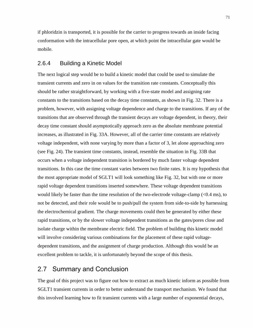
71
if phloridzin is transported, it is possible for the carrier to progress towards an inside facing
conformation with the intracellular pore open, at which point the intracellular gate would be
mobile.
2.6.4 Building a Kinetic Model
The next logical step would be to build a kinetic model that could be used to simulate the
transient currents and zero in on values for the transition rate constants. Conceptually this
should be rather straightforward, by working with a five-state model and assigning rate
constants to the transitions based on the decay time constants, as shown in Fig. 32. There is a
problem, however, with assigning voltage dependence and charge to the transitions. If any of the
transitions that are observed through the transient decays are voltage dependent, in theory, their
decay time constant should asymptotically approach zero as the absolute membrane potential
increases, as illustrated in Fig. 33A. However, all of the carrier time constants are relatively
voltage independent, with none varying by more than a factor of 3, let alone approaching zero
(see Fig. 24). The transient time constants, instead, resemble the situation in Fig. 33B that
occurs when a voltage independent transition is bordered by much faster voltage dependent
transitions. In this case the time constant varies between two finite rates. It is my hypothesis that
the most appropriate model of SGLT1 will look something like Fig. 32, but with one or more
rapid voltage dependent transitions inserted somewhere. These voltage dependent transitions
would likely be faster than the time resolution of the two-electrode voltage-clamp (<0.4 ms), to
not be detected, and their role would be to push/pull the system from side-to-side by harnessing
the electrochemical gradient. The charge movements could then be generated by either these
rapid transitions, or by the slower voltage independent transitions as the gates/pores close and
isolate charge within the membrane electric field. The problem of building this kinetic model
will involve considering various combinations for the placement of these rapid voltage-
dependent transitions, and the assignment of charge production. Although this would be an
excellent problem to tackle, it is unfortunately beyond the scope of this thesis.
2.7 Summary and Conclusion
The goal of this project was to figure out how to extract as much kinetic inform as possible from
SGLT1 transient currents in order to better understand the transport mechanism. We found that
this involved learning how to fit transient currents with a large number of exponential decays,

72
and evaluate the quality of these fits using a number of different measures, to find the right
number of terms. This analysis is laborious and time consuming, but the end result is kinetic
parameters that map one-to-one with conformational changes of the protein, insight that is not
available by any other means. In the process we discovered that a transient analysis with a
limited number of terms does not measure a subset of the decays, but instead provides a form of
weighted average that may not be indicative of the underlying mechanism—highlighting the
importance of using measures to test for the correct number of decays.
Although an emphasis is often placed on measuring the decay time constants, we found that they
contained minimal features and were, for the most part, voltage independent, while the
accompanying charges contained important information about the arrangement of the
transitions. The magnitude of each decay’s charge contribution is highly dependent on the
direction of the voltage jump, an observation that reinforces the need to use multiple holding
potentials to detect all the decays. This multi-holding strategy also provides a direct and easy
way to use these unequal directional charges to build a model of the transporter transitions, by
taking advantage of the masking effect that occurs when a slow transition hides a faster one.
Ultimately we end up with a linear five-state model with two slow transitions in the middle (25
and 50–150 ms) flanked by two faster ones (2 and 5 ms) on either end.
This kinetic data becomes significantly more relevant when combined with structural insight
into the gated rocker-switch mechanism of SGLT1 revealed by crystallographic studies of the
LeuT architecture superfamily. The gated rocker-switch mechanism predicts four
conformational changes, and the kinetic studies have confirmed this in an elegant way by
matching each gate and pore conformational change to a carrier decay. This reveals that the
gates move on the order of 2–5 ms while the pores are an order of magnitude slower at 25–150
ms. By looking within the crystal structure at the gate and pore structures in more detail, we can
form theories about how these mechanisms work on the atomic level by matching them with
their known rates. Going one step further, we can use strategic mutants to test these theories by
mapping a mutations effect back on to the structure by monitoring changes to the four carrier
decays. There is remarkable synergy between transient and crystallographic studies. Crystal
structures provide unparalleled structural information, while the transient kinetics provide
unparalleled dynamic information. Now, more than ever, it is important to reinvest in kinetic
studies to take advantage of the structures we now have and have waited so long for. This

73
analysis is general enough that it can be applied to any electrogenic cotransporters, and,
therefore, presents an opportunity to expose other mechanisms and possibly classify
cotransporter mechanisms kinetically.
2.8 Future Work
There are a quite a few different paths worth exploring with the transient currents kinetics that
are discussed in more detail below. These include simulations; verifying the connection between
the four predicted conformational changes and the four carrier decay components using strategic
mutants; expanding the analysis to involve substrate binding steps and explore the question of
binding order; study the kinetics of other carriers with the gated rocker-switch mechanism, as
well as other mechanisms.
2.8.1 Simulations
As discussed earlier in §2.6.4 Building a Kinetic Model, the path to building a state-model
simulation of SGLT1 has been laid out with a five–state model provided by the transient
kinetics. What remains is figuring out where to place the voltage dependent steps, and the
assignment of charge displacement, which should be possible by trying a number of different
configurations. This would be an important test of the transient model (fast-slow-slow-fast), as it
would demonstrate the capability of this model to produce the observed transient kinetics. It
would also provide a way to tune the rate constants through fitting and find more precise values.
It would be helpful to demonstrate the masking effect directly with a simple state model. A good
place to start would be a three-state model with one slow and one fast transition. However, there
are complications with the placement of voltage dependence. Adding voltage dependence
directly to either or both transitions makes their rate and time constants variable, and, therefore,
difficult to enforce separate transition rates. A better setup might be voltage independent fast
and slow transitions connected in the middle by a rapid voltage dependent transition that can
move the system from side to side. Once the model is built, large differences in rates could be
used to establish the masking effect and then these rates can be brought closer together to find a
threshold where the effect dissipates. It would also be interesting to compare the threshold for
the masking effect with the one for the rapid equilibrium assumption.

74
2.8.2 Strategic Mutants
Prior to the crystal structure of vSGLT quite a few SGLT1 mutations were characterized in an
effort to elucidate structure and function. Amongst these are several that cause uniquely
debilitating effects, which seem to indicate a malfunction of one of the carrier’s conformational
changes. Characterizing the transient kinetics of these mutants will help identify the affected
transition, much like the T156C mutant, and reveal the amino acid’s functional significance
within the tertiary structure. Carrying out this strategy over a series of mutants has the potential
to map each step of the gated rocker-switch mechanism to key residues of the architecture. Once
these associations are confirmed, the functional significance of new mutations can be
understood in a comprehensive way by looking at their effect on the four carrier conformational
changes.
Despite not being able to bind glucose or phloridzin the K157C mutant does generate transient
currents. Studying their kinetics should corroborate the findings of T156C and reveal the greater
extent of this mutation’s malfunction. While T156C retains minimal mobility of the transition
associated with component 4 (30 ms), it is our hunch that the K157C mutation will abolish it.
Component 4 is putatively related to movements of the extracellular pore, and an important
question is what other conformational changes can and cannot take place when this is
completely inhibited. This leads to ideas of coupling between the conformational changes and
how dependent they are on each other.
The Q457R mutation has been found to be the cause of glucose galactose malabsorption in some
patients. This mutant can bind glucose but is unable to transport it and transiently unbinds it,
suggesting an inability to orient to an inside facing conformation18
. It is likely that the
intracellular pore (decay 5, 150–50 ms) is unable to open, although it is also possible that the
extracellular pore cannot close to initiate transport. The vSGLT crystal shows that this residue
forms part of the galactose binding site with the amide group interacting directly with two
substrate oxygens68
. Furthermore this residue is responsible for turning hSGLT3 into a glucose
sensor67
. An earlier study of ours with three decays and 150 ms pulses found that this mutation
decreases the slowest component from 45 to 15 ms, seeming to indicate indirectly that decay 5
(150 ms), which we were not monitoring then, had disappeared190
. A full transient analysis
should confirm this and implicate the intracellular pore.

75
No mutations have been linked to the gating mechanisms of SGLT1 (except for an identified
F453L mutation in several GGM patients45
), yet it would be valuable to confirm that
components 2 (2 ms) and 3 (5 ms) monitor these processes. This should be possible by studying
conservative mutations of the intracellular (Y290) and extracellular gates (L87, F101, and
F453), such as swapping phenylalanine and tyrosine or leucine and isoleucine. We suggest
conservative mutations because we are only looking for a positive indicator, such as a change in
rate, that the associated component is affected. A more drastic mutation may cripple the carrier
in a way that makes it difficult to study.
A disulfide bridge has been identified between C255 and C51119
, which when disrupted by
mutating either or both residues (C255A, C511A, C255A/C511A), leads to transients in the
presence of glucose77
. This suggests difficulty orienting to an inside facing conformation similar
to Q457R. Characterizing any of these mutants and identifying the affected conformational
change can help with understanding the structural role of this disulfide bridge, and the roles
sulfur bridges play in conformational changes.
Mutations of residue D204 have a large impact on ion coupling and affinity, but most
significantly D204N turns the carrier into a glucose gated H+ channel with a H
+:glucose
stoichiometry as large as 145:1202
. It would be interesting to see what conformational changes
this residue affects, since the D204E mutation has already been shown to alter the transient
kinetics. Understanding how SGLT1 might be altered to take on channel-like properties can give
insight into possible conformations that would provide a channel-like pathway. D204N and
D204C are expressed poorly making D204E the best mutant to study.
A stretch of TM4 and its extracellular tip (143–180) has been studied by our group with cysteine
scanning mutagenesis17
, and a key series of residues (F163, A166, Q170, and K173) were found
to line one side of an alpha helix forming a surface of an extracellular pore that is thought to be
involved in Na+ interaction
15,188,189,203. Each of these mutations shifts the Q–V distribution (10–
20 mV) and double and triple mutants have an additive shifting effect (45–90 mV). To
understand the functional significance of this region we would investigate the kinetics of these
key mutants beginning with A166C because of its ~4 times higher αMG affinity, followed by
Q170C, K173C, and F163C.

76
2.8.3 Substrate Transients
A natural extension of the kinetic studies presented here would be to study how altering the
extracellular Na+ concentration affects each decay component. My hypothesis is that lowering
the extracellular Na+ concentration will decrease the rate of the extracellular gate (decay 3),
without significantly altering the other decays. This might give insight into how Na+ binds, and
if it is involved in a gating mechanism that exposes the binding site to glucose, since Na+ is
required to allow glucose to bind. Studying transient currents with the cut-open oocyte and zero
trans Na+ would also verify that there are four conformational changes in the complete absence
of Na+. The cut-open oocyte might also provide an opportunity to measure Na
+ binding directly
because of the faster settling time of the clamp.
Because substrates like glucose substantially diminish the transient signal, by promoting an
inside facing conformation where the carrier is electrically silent77,175
, most transient studies of
cotransporters are done in the absence of the non-ionic substrate. Some mutants, however, resist
an inside facing conformation, and this provides an opportunity to study substrate transients and
the steps immediately before and after binding. The Q457R mutant is perhaps the best example,
since transport is abolished but substrate binding is intact. However, the T156C mutant is
similar in its ability to transiently unbind phloridzin with depolarizing pulses. A strategy
designed around one or both of these mutants could identify new carrier conformations related
to substrate binding, and would also provide a great opportunity to study the elusive binding
order question, which has been debated since the dawn of SGLT1 kinetic studies. The
dependence of the transient parameters on glucose, phloridzin, and Na+ should provide enough
kinetic detail, if not the most available so far, for discriminating between the three competing
models (N/N/S, N/S/N, and N/random; N=Na+, S=glucose/phloridzin). The disulfide bridge
mutants (C255A, C511A, and C255A/C511A) are also potential candidates that generate
glucose transients, but in their case retain transport function. Lastly, the wt carrier generates
transients with some poorly transported substrates like indican175
.
2.8.4 Other Carriers and Mechanisms
Given that SGLT1 belongs to a larger structural superfamily that shares the LeuT architecture, it
would be valuable to confirm that other members participate in the same conformational
changes of the proposed gated rocker-switch mechanism. This would validate the findings from

77
SGLT1 and provide contrasting variations to help understand this class of transporters. A
number of other solute:sodium symporter members that have been vetted in the oocyte system
and are suited for this include SMIT1107
SMIT2105
, SMCT1116
, and NIS133
.
Perhaps more interesting though are members of the neurotransmitter:sodium symporter family,
such as GAT1178,204
and SERT205
, which are expressed well in oocytes and generate a slow ~150
ms decay similar to component 5 of SGT1, while also appearing to have faster decays that have
not yet been measured. These carriers are close relatives of the crystalized LeuT and have a high
biological interest because of their role in synaptic signaling and psychological disorders and
treatment. If the gated rocker-switch conformations can be identified in these carriers as well,
this will demonstrate a strategy for characterizing transport mechanisms kinetically.
This approach could also be extended to other carrier families to see if they share a similar
mechanism or adopt a unique one, with a number of candidates listed in 3.1.1 Historical
Perspective.
Of most value may be a member of the major facilitator superfamily. These carriers are
expected to operate with a rocker-switch mechanism, and so it is our prediction that they will
lack the faster gate transitions (2 and 5 ms). Unfortunately, because of difficulties being targeted
to the plasma membrane, these carriers have mostly evaded electrogenic study. However, a
recent study of purified LacY reconstituted in proteoliposomes with a solid-supported
membrane has been successful206
. Using concentration jumps this carrier generates decays on
the order of ~500 ms. Exponential analysis was not performed but from our observation there
appear to be two decays of ~50 and ~200 ms. There has also been success with inducing plasma
membrane expression of HMIT in oocytes with strategic mutations106,207
, and this perhaps
represents the best opportunity for a MFS carrier. This superfamily is of interest not only
because it is one of the largest, but because it contains the GLUT family of hexose facilitators,
and has a large number of crystalized members.
Lastly, there are the excitatory amino acid transporters (EAAT), which have been characterized
in oocytes182,208,209
and studied transiently193
. These carriers belong to the DAACS family,
which has a unique architecture identified by the Gltph crystal.

78
2.8.5 Miscellaneous
The T156C mutant appears to have reduced mobility of the extracellular pore, which makes it a
good candidate for crystal studies, similar to how LacY was originally crystalized with an
immobilizing mutation24
. However, it would be difficult to crystalize T156C (or K157C)
directly as mostly bacterial transporters have been crystalized so far. One option would be to try
and find the analogous amino acids in vSGLT, but there are no obvious candidates.
A compliment to the electrophysiology studies would be an analysis of fluorescent transients.
The big question would be to see if the same four transitions were present or if different
conformational changes were exposed. Also, by placing fluorescent tags on key areas associated
with each conformational change, each mechanism could be explored in more detail.
The multi-holding protocol is rather stressful on the oocytes, with many unable to endure it. To
decrease this stress it would be helpful to validate a reduced protocol. This could be achieved by
reducing the number of holding potentials, potentially to only two with one jump from each
side. Depending on how many holding potentials were used, one might lose the ability to
measure Q–V distributions as a function of the holding and test potential (Fig. 27), but this cost
might be acceptable if viable oocytes were easier to come by.

79
2.9 Figures
Fig. 13: Characteristics of the T156C mutant. (A) Phloridzin apparent affinity calculated from inhibition
of the Q–V distribution; titration to 200 μM for wt and 2000 μM for the T156C mutant. The wt apparent
affinity is voltage independent (1.6±0.6 μM, n=10), compared with a highly voltage dependent and
significantly reduced affinity for the T156C mutant (30±3 μM, n=9 plateau). The y-axis is linear from 0–
5 and 5–170 μM. (B) Normalized Q–V distributions (wt n=17, T156 n=16), and fits with a Boltzmann
function ( (
( ))⁄ ; wt , ; T156C , ). (C) Effect
of phloridzin on the transient produced by a −50 to 70 mV jump. Phloridzin progressively reduces the wt
transient without affecting the kinetics, characteristic of a tight binding inhibitor. In contrast, phloridzin
unbinds from the T156C mutant and produces a slow transient decay. Intermediate phloridzin
concentrations (5–100 μM) enhance this unbinding decay, but eventually larger concentrations (>500
μM) are able to overcome this effect and inhibit the carrier.

80
Fig. 14: Position of the T156 and K157 residues of SGLT1 in the vSGLT structure, where they
are represented by Val-141 and Asn-142. (A) looking at the collapsed extracellular pore. (B)
zoomed view from the same angle with extraneous TM’s removed. T156 and K157 appear to be
at the midpoint of TM 3, near the binding site of Na+ and glucose and forming an equidistant
triangle with both substrates.
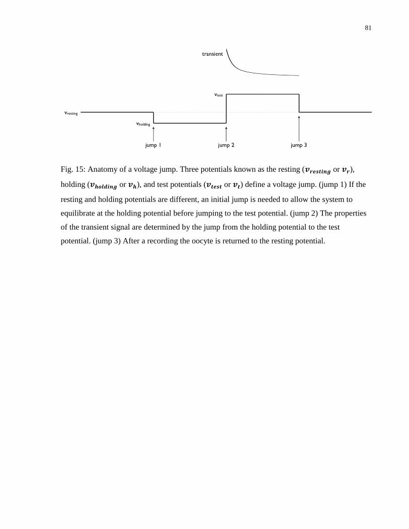
81
Fig. 15: Anatomy of a voltage jump. Three potentials known as the resting ( or ),
holding ( or ), and test potentials ( or ) define a voltage jump. (jump 1) If the
resting and holding potentials are different, an initial jump is needed to allow the system to
equilibrate at the holding potential before jumping to the test potential. (jump 2) The properties
of the transient signal are determined by the jump from the holding potential to the test
potential. (jump 3) After a recording the oocyte is returned to the resting potential.

82
Fig. 16: Relationship between voltage jumps and transient kinetics. (A) Two jumps with the
same test potential (30 mV) but different holding potentials (−150 and 70 mV) decay at the
same rate. (B) Reversing the jumps in A results in different kinetics because of the different test
potentials (red and blue charge movements are approximately equal). (C and D) Different
holding potentials can result in large variations in charge movement. Charge movements are
dependent on the voltage jump crossing the active region of the transporter (30 mV in this
example). Traces have been baseline adjusted, and absolute current values are plotted. Data is
from the T156C mutant.
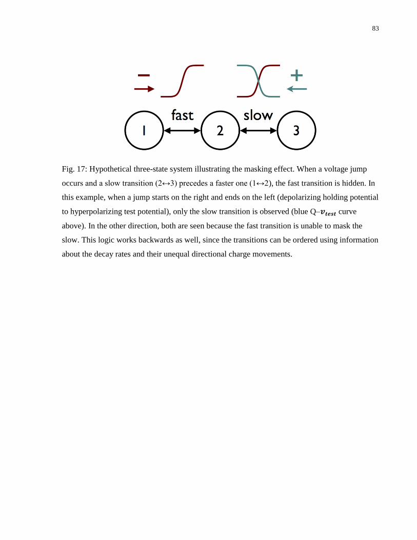
83
Fig. 17: Hypothetical three-state system illustrating the masking effect. When a voltage jump
occurs and a slow transition (2↔3) precedes a faster one (1↔2), the fast transition is hidden. In
this example, when a jump starts on the right and ends on the left (depolarizing holding potential
to hyperpolarizing test potential), only the slow transition is observed (blue Q– curve
above). In the other direction, both are seen because the fast transition is unable to mask the
slow. This logic works backwards as well, since the transitions can be ordered using information
about the decay rates and their unequal directional charge movements.

84
Fig. 18: Single and multi-holding voltage clamp protocols. (A) The voltage waveform of a single-
holding protocol with a −50 mV holding/resting potential shared by all twelve test potentials. (B)
Transient currents produced by A. (C) Multi-holding protocol for a −10 mV test potential with twelve
holding potentials. A phase has been inserted (0–300 ms) for transitioning between the resting and
holding potentials. Protocols for alternate test potentials are indicated by the grey waveforms. (D)
Transient currents produced by C. Orange traces show the data that would be analyzed with each type of
protocol to measure the kinetics at −10 mV. Data is from the T156C mutant.

85
Fig. 19: Example multi-holding data set. (A) Transient decays shown at full scale for jumps
from 23 holding potentials (−150…Δ10…70 mV) to a −50 mV test potential. The two shaded
regions are expanded in B and C to give a clearer view of the fast large-amplitude (B), and slow
low-amplitude (C) decays. The five furthest holding potentials on either end are colour coded
and labeled in B. Traces in C are smoothed using 100 nearest neighbor averaging (1 ms
window). Data is from the T156C mutant.
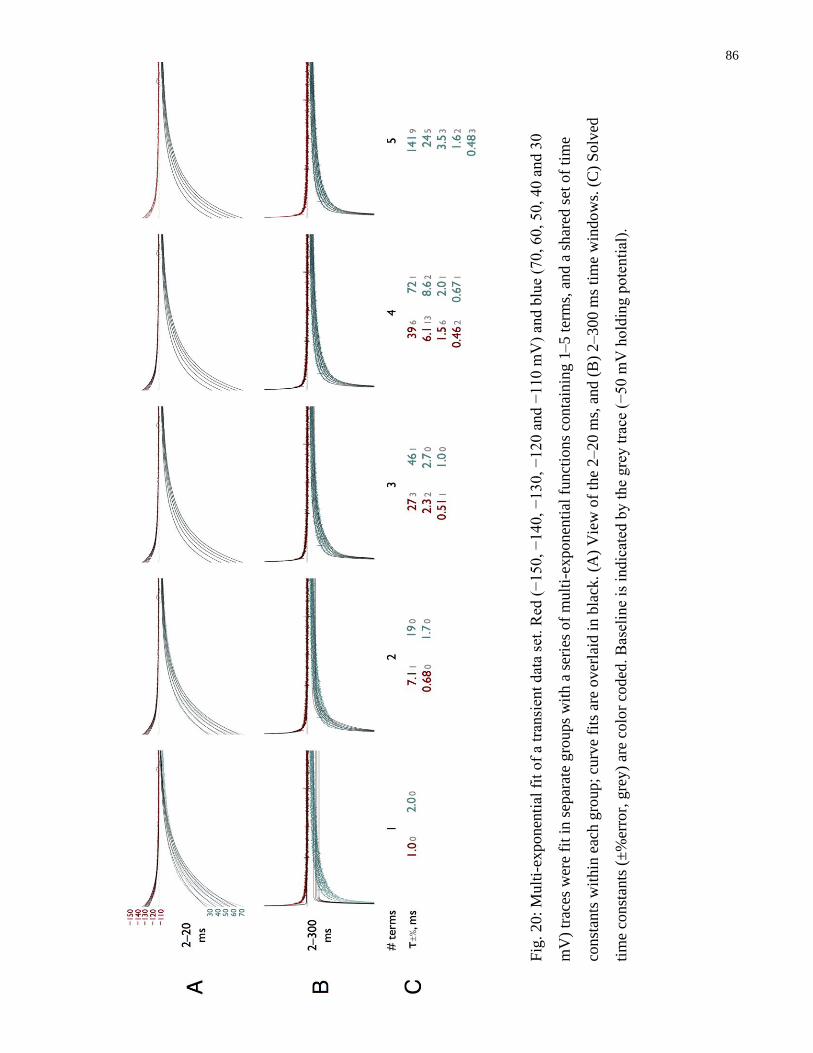
86
Fig
. 20:
Mult
i-ex
ponen
tial
fit
of
a tr
ansi
ent
dat
a se
t. R
ed (
−15
0,
−14
0,
−13
0,
−12
0 a
nd −
110
mV
) an
d b
lue
(70,
60,
50,
40 a
nd
30
mV
) tr
aces
wer
e fi
t in
sep
arat
e g
roups
wit
h a
ser
ies
of
mult
i-ex
po
nen
tial
fun
ctio
ns
conta
inin
g 1
–5 t
erm
s, a
nd
a s
har
ed s
et o
f ti
me
const
ants
wit
hin
eac
h g
roup
; cu
rve
fits
are
over
laid
in b
lack
. (A
) V
iew
of
the
2–20 m
s, a
nd (
B)
2–
300 m
s ti
me
win
dow
s. (
C)
Solv
ed
tim
e co
nst
ants
(±
%er
ror,
gre
y)
are
colo
r co
ded
. B
asel
ine
is i
ndic
ated
by t
he
gre
y t
race
(−
50 m
V h
old
ing p
ote
nti
al).

87
Fig
. 21:
Fit
res
idual
s. R
esid
ual
s ar
e sh
ow
n f
or
the
−150 a
nd 7
0 m
V h
old
ing p
ote
nti
als
wit
h 1
–6 t
erm
s. (
A a
nd B
) R
esid
ual
s dec
reas
e
as t
erm
s ar
e ad
ded
(χ2
indic
ated
), u
nti
l o
nly
nonse
nse
fit
s ar
e re
turn
ed (
fad
ed r
ed f
ive-
term
and b
lue
six
-ter
m).
Plo
ts a
re s
had
ed t
o
emphas
ize
dev
iati
ons
fro
m z
ero. D
ata
has
bee
n s
mooth
ed w
ith 1
00 n
eare
st n
eighbor
aver
agin
g (
1 m
s w
indow
).

88
Table 4: Nonsense fit examples. A variety of fit results are shown for the different nonsense cases that came up.
The fit parameters ± %error are shown along with the best χ2 that was achieved for each number of exponential
terms. The voltage jump is shown above each solution. (A) %error > 50% (beige shading). (B) χ2 greater than a fit
with fewer terms (green). (C) Low Q (grey) (<0.05 nC). (D) Low τ (yellow), and high Q (red). (E) High τ (orange).
(F) Some Q with opposite sign (blue). (G) Two τ converging (pink).

89
Table 5: Seeding examples for multi-exponential fitting of the hyperpolarizing jump dataset (Fig. 19,
blue). Final solutions are shown on the left for different numbers of exponential terms used in the fit
equation. To the right are parameter seeds that led successfully to the final solution, as well as seeds that
failed to arrive at a valid solution. Some failed fits are shown in two steps, with the initial seed followed
by the failed solution (grey shading). #I, number of iterations to final solution. Percent standard errors of
the fit parameters are shown in grey. Charge data is from the 70 mV holding potential trace.

90
Fig. 22: Transient charge movements by component. Charge/time-constant pairs from the −150
and 70 mV holding potential fits in Fig. 20 are displayed. (A) Charge magnitudes are shown as
horizontal bars positioned along a vertical and logarithmic time-constant scale. (B) The
corresponding data points are displayed in the table below. The failed 5 and 6-term fits are faded
and the invalidating parameter errors are shaded beige.
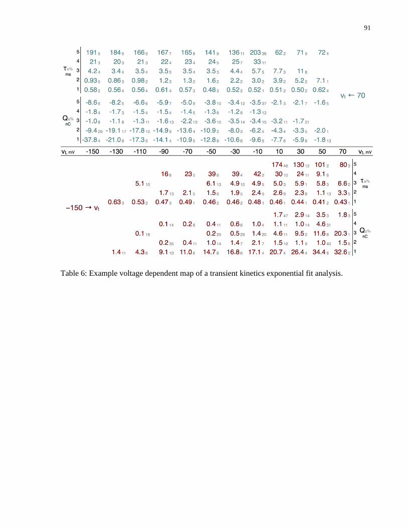
91
Table 6: Example voltage dependent map of a transient kinetics exponential fit analysis.

92
Fig. 23: Transient kinetics of SGLT1. Multi-exponential analysis of wt ±phloridzin (200 μM), T156C ±phloridzin (2000 μM), and non-injected oocyte transient currents.
Five decay at most were found (1–5). The charge (A) and time constant data (B) are shown for each decay as a function of the test potential and direction of the voltage jump
(depolarizing, red; hyperpolarizing, blue; total charge, black = red + blue). Decays are numbered by the rate of their decay (1, 0.4–0.85 ms; 2, 1–5 ms; 3, 2–12 ms; 4, 10–60 ms;
5, 60–380 ms).Decay 1 is produced by the membrane capacitance and decays 2–5 by the carrier. Top row: carrier charges are overlaid (B, 2–5), with the total in black indicating
the size of the free carrier pool; time constants are plotted on a logarithmic scale (A, 1–5). wt and non-injected experiments used a shorter voltage range (−130 to 50 mV) than
T156C (−150 to 70 mV) to reduce oocyte stress (see §2.2.4); also, their decay 2–5 charges are plotted on a smaller scale (15 nC) than T156C (30 nC) because of lower protein
expression. Two capacitive decays (grey and white filled) were observed at some depolarizing potentials for non-injected. Representative data sets are shown. The T156C data is
an average of three measurements in the same oocyte without phloridzin and two with; one measurement for wt ±phloridzin and control.
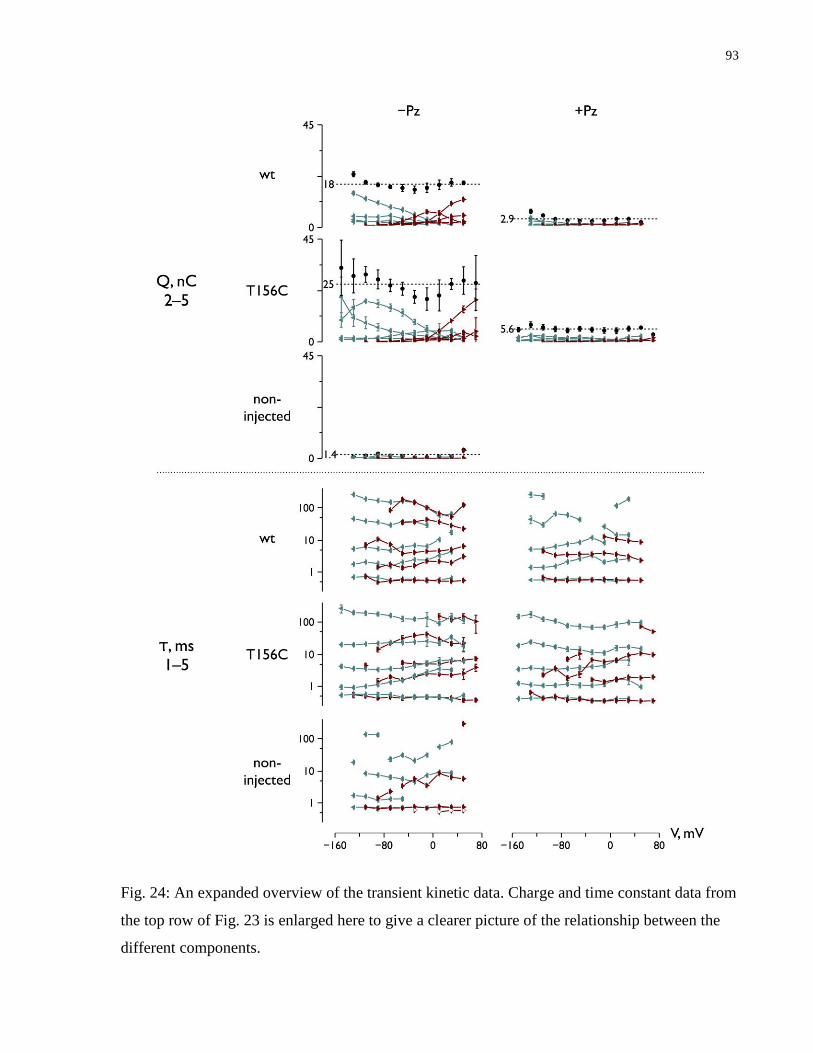
93
Fig. 24: An expanded overview of the transient kinetic data. Charge and time constant data from
the top row of Fig. 23 is enlarged here to give a clearer picture of the relationship between the
different components.

94
Fig. 25: Close up of the transient kinetic data given in Fig. 23. Each plot is expanded with its own ordinate scale
ranging between zero and the maximum indicated on the left.

95
Fig. 26: Changes in measured kinetics when fitting with limited exponential terms. The T156C mutant data set in the
absence of phloridzin, shown in Fig. 23, was analyzed with limited numbers of exponential terms (5–1, separate
columns decreasing to the right). As exponential terms are removed from the fit equation some decays are no longer
distinctly observed, and are instead absorbed by the others.

96
Fig. 27: Component charge dependence on the holding and test potential for the T156C mutant. In a second round
of fits the charge contributions of the intermediate holding potentials were found, for each test potential, as
described in the text. These dependencies were sigmoidal for the carrier (2–5) and linear for the capacitive (1), as
expected. The sigmoidal curves were fit with a two-state Boltzmann equation, fits shown, to obtain valence ( ) and
data for each decay as a function of the test potential, averages indicated on the figure; curves with insufficient
detail for fitting are faded. The component 4 curves separated into two pools with distinct ’s. The capacitive
data was fit with a line, fits shown, to find the membrane capacitance from the slope, average indicated.

97
Fig. 28: Additional wt and T156C transient kinetic data sets, in the absence of phloridzin. In Fig.
23–Fig. 25 data from a single oocyte is shown and reproduced here in column 1, while
additional data sets from the same or different oocytes are shown in columns 2 and 3. Charge
scales are indicated in each subplot.

98
Fig. 29: Arranging decay charge profiles using the masking effect. (A) The two slowest decays (4 and 5) are
placed side by side but there is an inconsistency with the large decay 4-red charge, which is expected to be
masked by 5 when moving from left to right. (B) The alternate arrangement is consistent and accepted. (C)
The faster decays (2 and 3) cannot be placed in the middle, in any arrangement, because the slow decays (4
and 5) on either end will mask them when moving in both directions. (D) 2-blue and 3-red generate more
charge in the same direction that they would be masked by the slow transitions in the middle (4 and 5). (E)
This arrangement makes the most sense as it is consistent with all the charge profiles.

99
Fig. 30: Assigning transient decays to conformational changes of the carrier predicted by the crystal model.
Conformational changes predicted by crystal structures sharing the SGLT1 architecture, as shown in Fig. 12, are
aligned with the decay charge profiles arranged in Fig. 29. Most of these states were captured in the presence of
substrate, but are expected to also occur when the empty carrier reorients between sides of the membrane. The two
fast decays on either end (3 and 2) align with the outside and inside gates, and the inner slow decays (4 and 5) with
movements of the two pores. The T156C data shows that decay 4, which is inhibited by the mutation, is associated
with opening/closing of the extracellular pore.
Fig. 31: Revised SGLT1 transport model. This model incorporates the four carrier conformational changes
predicted by the crystal and transient studies (Fig. 30), for reorientation of the carrier across the membrane, with the
classical model of ordered substrate binding (Fig. 1). Closed gates and pores are represented by black and maroon
bars, respectively.
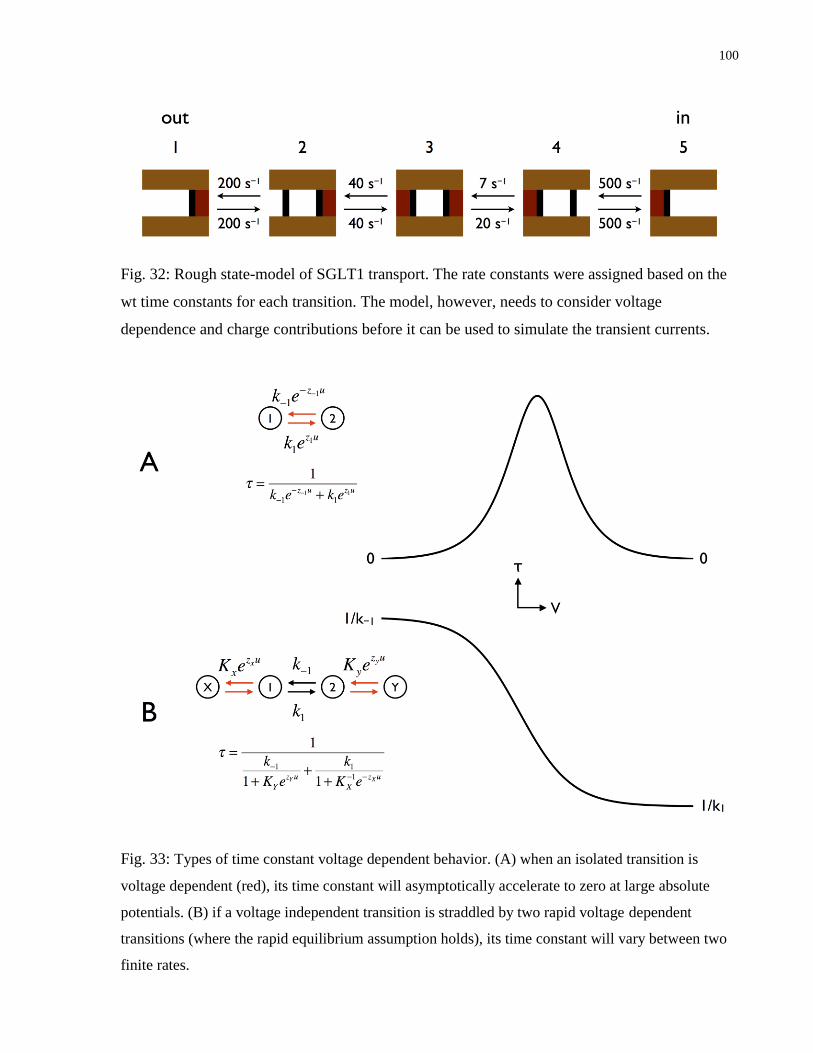
100
Fig. 32: Rough state-model of SGLT1 transport. The rate constants were assigned based on the
wt time constants for each transition. The model, however, needs to consider voltage
dependence and charge contributions before it can be used to simulate the transient currents.
Fig. 33: Types of time constant voltage dependent behavior. (A) when an isolated transition is
voltage dependent (red), its time constant will asymptotically accelerate to zero at large absolute
potentials. (B) if a voltage independent transition is straddled by two rapid voltage dependent
transitions (where the rapid equilibrium assumption holds), its time constant will vary between two
finite rates.

101
A Practical Method for Characterizing the Voltage 3
and Substrate Dependence of Membrane Transporter Steady-State Currents
3.1 Introduction
After the transient current subsides a transporter will continue to cycle in the presence of
transported substrate as it is acted upon by electrochemical forces. This cycling velocity ( ; is
used so that can be reserved for voltage) can be measured electrophysiologically by observing
the steady-state current generated as a net quantity of charged substrate is translocated across the
membrane. This cycling velocity is analogous to the turnover frequency (both with units of
cycles/second), and this rate is related to the membrane current by a scalar involving the number
of expressed carriers ( ), the net charge translocated per cycle ( ), and the elementary charge
( ),
Eq. 2
As stated above, the cycling velocity is driven by the electrochemical potential which is affected
by the concentration of transported substrates and the strength of the membrane potential.
Measuring the steady-state current while varying the membrane potential produces the familiar
I–V curves (Fig. 34A), which often have a sigmoidal voltage dependence that varies between a
maximum velocity at saturating voltage and zero. Titrating a transported substrate scales and
alters the shape of the I–V curve. Typical I–V studies are concerned with measuring the
standard Michaelis-Menten parameters , , and the Hill coefficient by analyzing, at
each voltage, the saturation curve as a function of substrate concentration (Fig. 34B). These
parameters are then often plotted as a function voltage to observe their voltage dependence.
The sigmoidal voltage dependence of the steady-state velocity curves is seldom analyzed,
because no methods of a general nature are available to do so, and the problem is generally
believed to be complex. There is, however, important kinetic information contained in the shape
of these curves that is wasted, especially considering that this data is commonly and easily
collected for substrate apparent affinity measurements. The goal of this project was to extract as

102
much kinetic information as possible from the steady-state velocity by modeling its voltage and
substrate dependence, and in so doing increase our understanding of how cotransporters work. A
general model will be presented that turns out to be rather simple, yet has broad applications to
the field of membrane transport. Using the concept of a general -state cyclical system, a
mathematical representation of the steady-state velocity will be derived, and its voltage and
substrate dependence described. It turns out that the steady-state velocity consists of a series of
terms that can be written down by following a simple recursive pattern. Furthermore, these
terms have units of time with the slowest ones of each type of dependence (voltage, substrate,
voltage and substrate, and none) dominate the expression under different conditions. This allows
the steady-state velocity equation to be reduced to a few terms that extend the Michaelis-Menten
equation to include voltage dependence. This reduced equation shows how the I–V curves can
be fit with the familiar Boltzmann equation, and this allows for a simple measurement of
valences ( ) and ’s, which are typically only obtainable from the transient currents.
3.1.1 Historical Perspective
A number of attempts at describing the properties of the I–V curves have been made, but they
have either been too specific, too complicated, or both, to be widely adopted. Some of the
earliest treatments were in the 70’s. Geck and Heinz derived a general n-state model210
, while
Stein used standard 3 and 4-state representations211
. In both derivations, they considered several
cases for assignment of the voltage dependent transitions, and described trends for some of the
parameters (linear, nonlinear, increasing, decreasing, etc.), with Stein noting that the expressions
were too complex to go into more detail. Other more specific derivations include a six-state
model of H+/substrate symport by Sanders et al.
212, a six-state model of ion coupled transport by
Lauger and Jauch213
, and a four-state model of ion pumps by Lauger focused on the shape of the
energy barrier214
.
Hansen et al. were among the first to describe the geometric properties of the curves
themselves215
. A reduced two-state model ignoring substrate was used, where all the voltage
independent steps were combined together and one voltage dependent step was used. They
considered the net velocity (forward and reverse velocities subtracted), and then used a change
of coordinate system and hyperbolic trigonometric functions to simplify the expression.

103
Although they did have success identifying symmetries, the expression remained too complex,
and the model too simple, to be of general use.
At the time of these earlier investigations quality I–V measurements were difficult to obtain, and
there was an emphasis on the saturation behavior at extreme potentials for pumps and
ionophores, such as currents measured from a Neurospora crassa H+ pump
216,217, a Na
+ pump in
sheep cardiac Purkinje fibres218
, active Na+ currents across frog skin
219, and ion transport by
valinomycin in lipid bilayers220
. Glucose activated currents were measured several years later in
intact epithelial cells with ionic control of the membrane potential221
, and in intact Necturus
small intestine222
.
The patch clamp technique was developed by Neher and colleagues in 1978223
, and during the
80’s grew in popularity for studying channels and pumps and measuring I–V curves, such as the
first I–V measurement of the Na+/K
+ pump in myocardial cells (1985)
224. Expression cloning
soon followed in 1987, and attention shifted towards characterizing various cloned transporters
and designed mutants, and interest in a mathematical solution of the I–V curves waned. The first
I–V measurements of SGLT1 expressed in oocytes were reported in 1990225
, and were soon
followed by a wide range of carrier proteins (in chronological order): GABA transporter
GAT1180,226
; serotonin transporter SERT181
; H+/hexose transporter STP1
183; pig SGLT3
61;
H+/peptide transporter PepT1
184,227; Na
+/myo-inositol transporter SMIT1
107; excitatory amino
acid transporter EAAT2182
; EAAC1208
; amino acid permease AAP1228
; H+/myo-inositol
transporter MIT229
; H+/sucrose transporter StSUT1
230; SGLT2
62; Na
+/I
− symporter NIS
133; type
II Na+/Pi cotransporter NaPi-5
231; NaPi-2
197,232; Xenopus SGLT1-like protein xSGLT1L
233;
Na+/multivitamin transporter SMVT
136; reverse SGLT1 transport
80,82; flounder renal high-
affinity-type Na+/dicarboxylate cotransporter fNADC-3
234; amino acid permease AAP2–6
235;
SMIT2105
; Na+/nucleoside transporter CNT1
236; Na
+/monocarboxylate transporter SMCT1
109,110;
NaPi-IIb237
; choline transporter CHT124
; CNT2238
; zebrafish Na+/monocarboxylate cotransporter
zSMCTe114
; CNT3187
.
With a plethora of kinetic data, and advancements in computing power, there was a shift in
emphasis towards model simulation and away from mathematical representations: SGLT1
rat239,240
, rabbit70,86,240-242
(D176A179
, Q170E189
, and BBMV76
), and human42,85,240
with
substrate77,175,243
and/or fluorescence175,243,244
; SGLT1 reverse transport82
; SGLT262
; SMIT1107
;

104
EAAC1193
; GAT1245
; PEPT1184
; StSUT1230
; NaPi-IIa197,232
; theoretical work246,247
. However, a
problem with these simulations is an inability to deduce fundamental properties of a system.
3.1.2 This Study
As mentioned above, earlier theoretical models of the steady-state velocity’s voltage and
substrate dependence have tended to rely on models tailored for a particular transporter. A
complex mathematical expression would typically be derived, and its characteristic studied for
different configurations of the voltage and substrate dependent steps. This task, however, is
laborious, requires a significant level of expertise, and can ultimately be futile if the wrong
model is chosen. In this study we have instead considered a general -state cycle without
limiting the placement of substrate and voltage dependent steps, as discussed in §3.2 Steady-
State Velocity of a Cyclical Model. This ends up making the derivation easier because we can
focus on overarching patterns as opposed to complex rate constant products. The trick is in
realizing that term in the general velocity equation can be conceptualized as a recursive family
of patterns. The effect voltage has on this equation is considered in §3.3.1 Introducing Voltage
Dependence and §3.3.2 The General Voltage Dependent Equation, and the geometric properties
of this curve are explored through examples in §3.3.3 Geometric Properties of the I–V Curves.
The ultimate conclusion from this section is that voltage dependence transforms the
denominator of the steady-state velocity equation into a series of voltage dependent exponential
terms, yet, in most cases, a single exponential term dominates and allows the others to be
ignored, resulting in the familiar Boltzmann function. This provides a phenomenological
method for characterizing the I–V curves by fitting them with Boltzmann functions, as is shown
later. Substrate dependence is considered in §3.4 Substrate Dependence, where we see how
changing the substrate concentration shifts the exponential denominator terms, and in so doing
can change the dominant exponential term. Lastly in §3.5 Results, steady-state data from our lab
for SGLT1 and other carriers taken from the literature are fit with Boltzmann functions and a
mathematical model is constructed. We see how this model can be related back to the original
cycle and few rate limiting patterns. To provide simple examples mostly finite models are
considered in the main text, while general derivations are given in §3.7 Appendix.

105
3.2 Steady-State Velocity of a Cyclical Model
Often transporters can be represented by a simple cycle, if substrate interactions are ordered and
leak pathways are small12,175,215,248. The general case is accounted for by the -state cycle
shown in Fig. 35. The steady-state velocity of this system is well defined (Eq. 29) and is derived
in the Appendix (§3.8.1 Deriving and Arranging the Steady-State Equation). However, for our
purposes all that is important is the form of this equation, which is easier to demonstrate with
the small three-state cycle shown in Fig. 36. Understanding these patterns will clarify the
general solution and help later on when we introduce voltage dependence.
The steady-state velocity ( ) of any cycle can be separated into counterclockwise ( ) and
clockwise ( ) componentsf,
Eq. 3
which have the following solution for the three-state system in Fig. 36,
( )
( )
( )
(
)
(
)
(
)
Eq. 4
with,
Eq. 5
f (rate) is used for the steady-state velocity so that and can be reserved for voltage and sigma notation,
respectively.
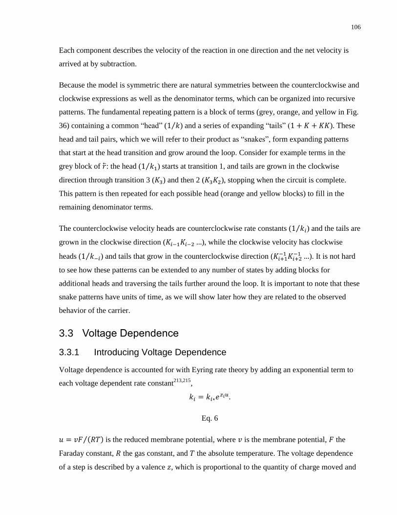
106
Each component describes the velocity of the reaction in one direction and the net velocity is
arrived at by subtraction.
Because the model is symmetric there are natural symmetries between the counterclockwise and
clockwise expressions as well as the denominator terms, which can be organized into recursive
patterns. The fundamental repeating pattern is a block of terms (grey, orange, and yellow in Fig.
36) containing a common “head” ( ⁄ ) and a series of expanding “tails” ( ). These
head and tail pairs, which we will refer to their product as “snakes”, form expanding patterns
that start at the head transition and grow around the loop. Consider for example terms in the
grey block of : the head ( ⁄ ) starts at transition 1, and tails are grown in the clockwise
direction through transition 3 ( ) and then 2 ( ), stopping when the circuit is complete.
This pattern is then repeated for each possible head (orange and yellow blocks) to fill in the
remaining denominator terms.
The counterclockwise velocity heads are counterclockwise rate constants ( ⁄ ) and the tails are
grown in the clockwise direction ( ), while the clockwise velocity has clockwise
heads ( ⁄ ) and tails that grow in the counterclockwise direction (
). It is not hard
to see how these patterns can be extended to any number of states by adding blocks for
additional heads and traversing the tails further around the loop. It is important to note that these
snake patterns have units of time, as we will show later how they are related to the observed
behavior of the carrier.
3.3 Voltage Dependence
3.3.1 Introducing Voltage Dependence
Voltage dependence is accounted for with Eyring rate theory by adding an exponential term to
each voltage dependent rate constant213,215
,
Eq. 6
( )⁄ is the reduced membrane potential, where is the membrane potential, the
Faraday constant, the gas constant, and the absolute temperature. The voltage dependence
of a step is described by a valence , which is proportional to the quantity of charge moved and

107
the fraction of the field crossed, and when the voltage is zero the rate constant reduces to ;
this notation is also used for the and factors.
To see what effect Eq. 6 has on the velocities we can substitute it into one of the blocks in Eq. 4
(grey),
( ( )
( ) ( ) )
( ( )
( ) ( ) )
Eq. 7
By combining coefficients and exponents each term can be reduced to a simple exponential
( ), and because all blocks behave the same, and larger cycles will just have more terms, the
general form of these velocities is an inverted series,
∑
Eq. 8
Since all , the greatest effect on these curves’ behavior is the signs of the exponents
determined by . If the signs are all the same, the curves will be monotonically increasing
( ) or decreasing ( ) with increasing . However, with a mixture they will switch
between increasing and decreasing, and be much harder to describe in a general way.
For the remainder of this discussion we will only consider the behavior of curves similar to Eq.
8 without mixed signs. In practice this includes any carriers that have monotonic I–V curves,
and excludes those that demonstrate biphasic behavior. Fortunately, most carriers that transport
like-charged substrates, such as SGLT1, have monotonic curves, while some pumps have
biphasic curves. This condition is achieved by restricting the valences of rate constants in each

108
direction around the loop to opposite signsg. This implies that all the rate constants around each
loop accelerate with the same polarity, and that the two loops have opposite polarity.
The convention is for models to rotate counterclockwise at negative potentials, which occurs
when,
Eq. 9
and this will be the orientation that we adopt for the rest of this discussion.
3.3.2 The General Voltage Dependent Equation
Eq. 8 can be written in a more general and simplified form by considering voltage independent
terms ( and ), and moving their coefficients into the exponents to be expressed as horizontal
shifts ( and ) as outlined in §3.8.2 Simplifying the Voltage Dependent Expressions,
⁄
∑ ( )
⁄
∑ ( )
Eq. 10
where,
(
)
(
)
Eq. 11
g This becomes clear when we examine the form of the exponents in Eq. 7 for ( or ) and ( or
).

109
Reduced voltage dependent terms have combined valences ( and ) and coefficients ( and
),while the reduced voltage independent terms have been grouped together ( ∑ and
∑ ), and limit the maximum velocity in both directions ( ⁄ and ⁄ ).
3.3.2.1 Example 1
The steady-state velocities of the three-state model in Fig. 37 will be solved for and arranged
into the form of Eq. 10. We will begin by writing down the head and tail pairs using the patterns
illustrated in Fig. 36,
(
)
(
)
(
)
(
)
(
)
(
)
Eq. 12
and then collect and reduce the terms,
Eq. 13
Finally the voltage independent terms are rearranged and the amplitudes are brought into the
exponent,
( ) ( )
( ) ( )
Eq. 14

110
3.3.3 Geometric Properties of the I–V Curves
The steady-state expressions in Eq. 10 are sigmoid-like functions, ( ( ))⁄ , but with
the potential for multiple exponential terms in the denominator instead of just one. Since the
counterclockwise and clockwise expressions have the same form, and are simply reflections of
one another in the y-axis, we will only consider the counterclockwise velocity. As we will show,
the shape of most I–V curves can be accounted for by one or two terms, and so it helps to study
their geometric properties.
With one term the curve is a simple sigmoid, as shown in Fig. 38. It varies asymptotically
between 1 and 0, reaching its midpoint and steepest part at . For the rest of this
discussion we will use the notation and instead of and , because it is simpler to
write, but also because in the presence of multiple denominator terms it is not necessarily the
value of or that results in half maximal velocity. The majority of change (90%) occurs
within a band ( ⁄ ) on either side of , with the band becoming smaller, and the
slope steeper, as increases. In this way, and describe the curve’s voltage dependence.
3.3.3.1 Last Man Standing
If we think about the steady-state velocity equation in terms of the denominator terms (Eq. 4),
and recall that they represent snake patterns with units of time, we can see that the voltage
dependent patterns are infinitely slow at depolarizing potentials and increase in speed
exponentially to zero at hyperpolarizing potentials. In turn, the steady-state velocity starts off
negligible at depolarizing potentials and speeds up as the patterns become faster with
hyperpolarization. This behavior is illustrated in Fig. 39, which shows that when there are
multiple voltage dependent terms in the denominator the one with the most negative is the
last to speed up and therefore has the largest impact on the shape of the curve. If we examine the
curve at depolarizing potentials and move negative, we see that at all the terms are to the
right of their and much larger than 1, forcing the expression to 0. The first term reaches its
at , and drops to 1, but the other two terms are still large and the expression remains 0; this
is repeated again for the second term at . Only when the last term reaches its at
does this exponential series approach 1 and the curve begins to rise. This shows how even
though there may be many exponential terms in the velocity equation, often the one with the
most negative is dominant.

111
3.3.3.2 Overlapping Terms
Sometimes two terms can contribute to the shape of the velocity curve, if they have the most-
negative ’s and their bands overlap. An example of this behavior is shown in Fig. 40
for a low valence ( ) and high valence ( ) term. This large difference in valences is
needed to see the properties of both curves. In real systems the range of valences is usually
much smaller (0–2), and therefore it may be difficult to see the properties of more than one. In
this example the low valence (red) is held fixed while the high valence (blue) is shifted to
observe the effect this has on the compound curve (black). Because the compound curve is
limited by both terms, it can be drawn heuristically by tracing a path along the lower of the two.
The shallow slope and wider band of the low valence term ( ) forces the high valence to fit
underneath it. This results in a combined curve that has properties of the high valence term on
the right and the low valence on the left. This combined curve usually has one inflection point,
but if the high valence term is far enough to the right there will be three; one from each sigmoid
and another connecting them.
3.3.3.3 Example 2
Solving the model in Fig. 41 results in the following velocity equations,
( )
( )
Eq. 15
which are plotted along with the net velocity. The counterclockwise velocity has three inflection
points (green dots), because the higher valence term is far enough to the right ( ). In
contrast, the clockwise velocity only has one (red dot), because the two terms have similar
valences (−5.5 and −5) and are close together ( ). Notice that at extreme potentials
the net velocity approaches the directional velocities, as the opposing velocity becomes
negligible.

112
3.4 Substrate Dependence
3.4.1 Introducing Substrate Dependence
To see how substrate affects the denominator terms it will help to recall some examples from
Eq. 4,
Eq. 16
An important feature of these, and all the other terms, is the separation of counterclockwise and
clockwise rate constants across the numerator and denominator. If one substrate binding event is
introduced in each direction, we would need to consider three dependencies ( , independent,
), and for two binding events five ( , , independent, , ).
This many cases become cumbersome, and so a practical way to reduce them is to only consider
substrate binding in one direction. This simplification is used in the Michaelis-Menten
derivation and is natural since most I–V measurements are made under conditions that attempt
to minimize reverse transport, such as low intracellular substrate concentrations. We will
therefore limit this discussion to the counterclockwise velocity (i.e. forward transport) with
binding events in the counterclockwise direction.
Substrate dependence for one binding event can be added to the counterclockwise velocity in
Eq. 10 by adding voltage dependent (
) and independent (
) terms with a ⁄
dependence, as described in §3.8.3 Simplifying the Substrate Dependent Expression.
∑ ( ) ∑ (
)
Eq. 17

113
where,
and,
(
)
(
)
Eq. 18
This results in a maximum velocity that scales with substrate, , and two types of
exponential terms with different exponential shifts, and .
3.4.2 Characteristics of Substrate Dependence
Unsurprisingly, from Eq. 18 follows Michaelis-Menten kinetics,
where,
Eq. 19
as it represents the substrate dependence of the steady-state velocity at saturating voltage. This
shows that the maximum velocity at saturating voltage and substrate, , is governed by the
sum of the non-dependent (voltage/substrate independent) snake patterns ( ), while depends
on the ratio of the non-dependent and substrate dependent ( ) patterns (see Eq. 36).

114
The two exponential shifts in Eq. 18 have logarithmic substrate dependencies that can be
expressed in a simplified from as,
(
)
( )
Eq. 20
Terms representing voltage dependent snake patterns shift negative ( ), while those for
voltage/substrate dependent patterns shift positive ( ) as increases, as illustrated in Fig. 42.
The ’s of the voltage dependent terms decrease from infinity to a plateau of ( ) (red),
while the ’s of the voltage/substrate dependent terms increase from ( ) to infinity (blue).
This tells us that at low a voltage/substrate dependent exponential term will have the most
negative and be dominant, while at high a voltage dependent term will take over the
dominant role.
A special case occurs when the substrate binding step is voltage dependent, because none of the
substrate dependent snake terms will be voltage independent, and . This alters the
expressions,
⁄
(
) ( )
(
) ( )
Eq. 21
The maximum velocity loses its substrate dependence, since voltage can compensate for low
substrate concentrations. The ’s of the voltage dependent snake terms become substrate
independent, while the ’s of the voltage/substrate dependent terms now increase from
negative infinity to positive infinity.

115
3.4.2.1 Example 3
Some substrate dependent properties of the I–V curves are demonstrated with the examples in
Fig. 43. The model in Fig. 41, originally used to demonstrate voltage dependence, is modified
by adding a substrate binding event to either the voltage dependent transition (2→3) or the one
following it (3→1). The substrate dependence of the – curves is shown in A, and trajectories
of the – curves are in B; the paths followed by the are also overlaid in A.
In case 1, the substrate binding event is voltage dependent, and, therefore, is constant and
both increase (shift to the right) with increasing (see Eq. 21). At low concentrations (0.01–
0.1) is more negative and dominates, and the curve has a shallow slope ( ), but as
increases (1–10) the bands overlap (see B) and ’s steeper valence ( ) begins to
appear. Eventually is passed by (≥100) and becomes the most negative and dominant
term.
In case 2, substrate binding is voltage independent, and we see an that increases with
and a decreasing in (see Eq. 19 and Eq. 20). Over most substrate concentrations all three
bands overlap (0.01–1000, B) and both valences (0.5 and 5.5) appear in the – curves (A).
Only at very large concentrations (1000–1000×105) does drift above the band and slowly
disappear.
3.5 Results
3.5.1 Characterizing Experimental Data
To test the theory derived above, we analyzed substrate titration I–V data for a number of
cotransporters that are shown in Fig. 44A. The glutamine to cysteine mutant at position 170 of
rSGLT1 (Q170C) studied by our lab, and data digitized from the literature for the
2Na+/nucleoside human concentrative nucleoside transporter 3 (hCNT3)
187, hSGLT1
249, and the
3Na+/Pi rat renal type II cotransporter (NaPi-2)
197. These sigmoidal I–V curves were fit with a
Boltzmann function, ( ( ))⁄ , to measure a substrate dependent series of ’s
and ’s.
All of the carriers besides hCNT3 responded similarly, in that their ’s were relatively substrate
independent and their ’s initially followed an increasing trajectory (blue) and then plateaued

116
(red line). This increasing trajectory can be attributed to a positive shifting of the dominant
exponential term (see Fig. 42). Eventually, however, this positive shifting term passes another
exponential term that is following a negative, or flat, trend that has plateaued, and which
becomes the new dominant term. As shown, the increasing trajectory was fit with a logarithmic
function, ( ) ⁄ , to measure its parameters. However, only the Q170C with Na+
trajectory had enough detail to solve for , while the others, instead, used the average values
from B.
In the case of hCNT3 the dropped rapidly (3.5–0.5) as the substrate concentration increased.
This indicates that the dominant exponential term is replaced multiple times with lower valence
terms as the substrate concentration increases. Because the dominant term is changing, the
decreasing trajectory cannot be fit, and instead shows the ’s of several different terms as
they shift negative and take over the dominant position.
In the case of Q170C and hCNT3, where the charged substrate Na+ was used, we can tell that
Na+ binding to Q170C is voltage dependent because of its substrate independent . On the
other hand, Na+ binding to hCNT3 is clearly voltage independent because is substrate
dependent and the shifts negative. These findings provide clues about the pathway to the Na+
binding site, in that SGLT1’s is likely narrower, causing Na+ to sense the membrane electric
field, while hCNT3’s is wider and open to the extracellular environment.
3.5.2 Modeling the Steady-State Velocity
If we look at the general form of the steady-state velocity from Eq. 35, which is reproduced
below,
∑
∑
∑
∑
Eq. 22
we see that the series of terms in the denominator have different combinations of dependence on
substrate and voltage (none, , , and ). These terms come about from the snake patterns
which are then grouped based on these dependencies. As discussed in §3.4.2 Characteristics of

117
Substrate Dependence, ∑ and ∑
are related to the standard Michaelis-Menten parameters
, and (see Eq. 19 and Eq. 36), and can be calculated from them,
∑
∑
{
Eq. 23
When substrate binding is voltage dependent there is no ∑
term. We also know that, often,
one of the voltage dependent terms will be dominant, and so we can simplify Eq. 22 by
considering just one of each type of voltage dependent term,
∑
∑
Eq. 24
At low substrate concentrations,
is the dominant voltage dependent term, because
substrate is rate limiting and it represents the slowest substrate/voltage dependent snake pattern.
As substrate increases this term shifts positive following the blue trajectories in Fig. 44 (Eq. 20
or Eq. 21). Eventually, though, substrate stops being rate limiting and , which either shifts
negative or is substrate independent, becomes dominant, as it becomes the slowest voltage
dependent snake pattern (red dotted lines in Fig. 44). Looking at these different regions, we can
use the and information from the I–V fits, along with Eq. 39 and Eq. 20, to calculate the
remaining snake patterns,
Eq. 25

118
where is the saturating indicated by the red dotted line, and and are from the
logarithmic fit of the upward trajectory indicated by the blue line. The results of these
calculations are shown for several of the data sets in Fig. 45, and then used to construct a model
of the steady-state velocity equation using published and data. The calculation of
using always gave better simulation results and were therefore used, likely because of
inaccuracy in measuring the logarithmic slope ( ) with such few data points. The simulated
curves are in good agreement with the original data. This confirms that the steady-state velocity
can be modeled simply with one term of each type of dependence in the denominator (none, ,
, and ), and that the two voltage dependent terms ( and ) switch dominance as substrate
increases and ceases to be rate limiting. The Q170C rSGLT1 simulation deviated slightly at low
Na+ concentrations, indicating that a ⁄ term might be needed since two Na
+ ions bind to
SGLT1.
What is remarkable about these findings is that steady-state velocity gives information about
rate limiting snake patterns in the cycle, and that under different combinations of saturating
substrate and voltage conditions, different snake patterns are revealed. It appears that these rate
limiting snake patterns are the most that can be observed with the steady-state velocity, because
the rest of the patterns are faster and remain hidden. The voltage dependent terms and
are natural extensions of the Michaelis-Menten equation that take into account voltage
dependence.
3.6 Summary and Conclusion
The substrate dependence of the steady-state velocity has been of interest in enzyme kinetics for
over a century, marked most significantly by the publication of the Michaelis-Menten equation
in 1913250
. These studies are fundamental for characterizing substrate apparent affinities,
cooperativity, and turnover. With membrane transporters, their location within the membrane
provides a unique opportunity to study the ability of voltage to accelerate the cycling velocity,
and indirectly the voltage dependent transitions, using electrophysiological techniques.
Expression cloning has facilitated these types of studies and the measurement of the familiar
sigmoidal I–V curves. However, the approach to studying their kinetics is largely unchanged
from the classical Michaelis-Menten (or Hill) methods. The Michaelis-Menten parameters are
measured separately at each membrane potential to gauge their voltage dependence, yet the
119
sigmoidal shape of the I–V curves have remained mostly unexplored. Most attempts at
describing the I–V curves have failed because of the inherent complexity of the steady-state
velocity expression, which grows geometrically with the size of the model, and the added
complexity of working with exponential terms introduced through voltage dependence.
In order to get at the kinetic information contained within the I–V curves, we studied the
patterns formed by the denominator terms of a general -state cycle. The trick was in realizing
that these terms can be written down by following a simple recursive pattern, using the concept
of head and tail pairs. Conceptually, these snake terms have units of time and so the slowest
term, which corresponds with a pattern in the model, dominates the others and allows the
velocity expression to be greatly reduced. The reduced velocity expression is a simple
Boltzmann function, with one exponential term in the denominator, and provides a
straightforward phenomenological method for characterizing the I–V curves, by measuring their
’s and ’s. Not only is this analysis easy to do, but it provides a way to obtain and data—
which normally have required transient studies—from steady-state data that is often readily
available from apparent affinity measurements. We can go one step further and use this and
data, in combination with the Michaelis-Menten parameters, to calculate the values of these rate
limiting terms and build a reduced/equivalent model of the carriers voltage and substrate
dependence. This provides additional measures for characterizing and comparing transporters
and their mutants. These voltage dependent terms and are a natural extension of
the Michaelis-Menten parameters (∑ ⁄ and ∑
⁄ ) into the voltage
dependent space. The ultimate finding is that the steady-state velocity provides access to these
rate limiting snake patterns, which are also the most we can extract from the I–V curves. The
next step would be to try and build a model of the transport loop by guessing at the rate limiting
patterns and using them as building blocks.
3.7 Future Work
This project began because several SGLT1 mutants we were studying had highly voltage
dependent apparent affinities for Na+ and αMG and we wanted to model this behavior, thinking
that it might give insight into substrate binding order (see Fig. 46). At first the models designed
were specific to SGLT1, much like earlier theoretical studies, but this approach turned out to be
difficult and cumbersome. Eventually, on the suggestion of Dr. Backx, we began modeling the

120
steady-state current, thinking that it could be used to understand the apparent affinities. This
project is a completion of that steady-state work, and it would make sense now to return to the
apparent affinities, as they may contain additional information. It should be relatively straight
forward to model the apparent affinity as the expression is directly related to the steady-state
velocity (when , ⁄ ).
Ideally, it would be great to do a comprehensive experimental study of a cotransporter’s
kinetics, to validate the theory further and gain a deeper understanding of the carrier. With a
carrier like SGLT1, titrating with both substrates (Na+ and glucose) would provide information
on six–eight snake patterns (none, , , , , , , ; Na= , glucose= , voltage= ).
Using the cut-open oocyte, these measurements could be made in the forward and reverse
directions with complete control over the intra and extracellular substrate concentrations. This
would allow the destination solution to be clamped at zero substrate to eliminate reverse
transport and give more accurate readings. Working with patterns in both directions, it might be
possible to piece them together into a model of the carrier’s cycle by taking into account
substrate binding order and the relationships between the substrate dependent terms. The end
result would be simplified rate equations in both directions, and a full model built from the
patterns. Experiments with substrate on both sides of the membrane could then be used to test
these models in a mixed mode that they were not designed for.
3.8 Appendix
3.8.1 Deriving and Arranging the Steady-State Equation
Working with the three-state system in Fig. 36, we will first show how to transform the standard
form of the steady-state equation into one that is more useful for a voltage dependent analysis,
and then extrapolate to the general case.
The steady-state velocity equation in its general form,
∑
∑
Eq. 26

121
can be written down directly using the schematic methods of Wong–Hanes for the numerator
terms (∑ ), and King–Altman for the denominator (∑ )251,
Eq. 27
The net velocity, , is then split into forward and reverse components,
Eq. 28
which are each divided by their numerator and organized to arrive at the form in Eq. 4.
The patterns displayed in Eq. 4, and described in §3.2 Steady-State Velocity of a Cyclical Model,
can then be extended to the general case with states (see Fig. 35).
∑ [
( ∑ ∏
)]
∑ [
( ∑ ∏
)]
Eq. 29
Because the model is cyclical, indices in Eq. 29 that fall outside the range , need to be
mapped using modular arithmetic.
3.8.2 Simplifying the Voltage Dependent Expressions
We can express Eq. 8 in a more formal way by considering voltage independent terms and
writings separate expressions for the counterclockwise and clockwise velocities,

122
∑ ∑
∑ ∑
Eq. 30
Voltage dependent terms have combined valences ( and ) and combined coefficients with a
notation ( and
). The voltage independent terms ( and ) come about if there is at
least one voltage independent step in either directionh. Eq. 30 can then be simplified by
grouping the voltage independent terms,
∑
∑
Eq. 31
moving them into the numerator,
⁄
∑
⁄
∑
Eq. 32
and then bringing the new exponential coefficients into the exponents to be expressed as
horizontal shiftsi,
h For example, if the rate constants and are voltage independent, there will be a ⁄ term in and a ⁄
term in .
i ( ),
(
).

123
⁄
∑ ( )
⁄
∑ ( )
Eq. 33
where,
(
)
(
)
Eq. 34
3.8.3 Simplifying the Substrate Dependent Expression
To add substrate dependence for one binding event to the counterclockwise velocity in Eq. 30,
we need to include voltage dependent (
∑
) and independent (
∑
) snake terms
with a ⁄ dependence,
∑
∑
∑
∑
Eq. 35
The voltage independent terms can then be grouped,
∑
∑
Eq. 36
moved,

124
(
)⁄
∑
∑
Eq. 37
and the new coefficients brought into the exponents as shifts,
(
)⁄
∑ ( ) ∑ (
)
Eq. 38
where,
(
)
(
)
Eq. 39
3.8.4 Two Substrate Binding Events
Extending the derivation in Eq. 35–Eq. 39 to two binding events adds a quadratic term,
(
)⁄
∑ ( ) ∑ (
) ∑
(
)
Eq. 40
where,

125
(
)
(
)
(
)
Eq. 41

126
3.9 Figures
Fig. 34: (A) Example I–V curves measured over a range of substrate concentrations. (B) At each
potential the saturating I–s curves are fit to the Michaelis-Menten or Hill equation to determine
, and . Data is from the Q170C mutant of rSGLT1.

127
Fig. 35: General -state cyclical model.

128
Fig. 36: Example showing the form of the steady-state equation. The three-state model at the top is used to
illustrate these patterns for the steady-state velocity ( ), which has been split into the counterclockwise ( ) and
clockwise ( ) expressions written in full below. The denominator terms are organized into blocks of repeating
patterns that are colour coded to match the diagrams. The diagrams show how the terms within each block can be
generated iteratively by starting with a head term ( ⁄ ) and then growing the tail (∏ ) in a cyclical pattern until
the model is traversed. Note the symmetry between the and patterns, and how there is one block for each
possible head term. This pattern is easily applied to larger models by adding more blocks and extending the tails
around a larger loop.

129
Fig. 37: Example 1. Three-state model used to demonstrate a solution of the voltage dependent
general velocity equation.
Fig. 38: Geometric properties of a sigmoid function. The curve varies asymptotically between 1
and 0, reaching half-height at where it is also the steepest (slope, ⁄ ). A majority of
the change in magnitude (90%) occurs within the band .

130
Fig. 39: Effect of a dominant denominator term. With multiple exponential terms in the
denominator the one with the most negative dominates. The bottom expression is plotted and
evaluated at different values of . As terms pass their ’s they drop from to 1 to 0. When the
last term passes its the others are already small and the curve begins to rise.

131
Fig. 40: Geometric properties of a sigmoid function with two terms. A composite sigmoid
(black) contains two exponential terms, a low valence ( ) and high valence ( ).
Separate curves are also drawn for single term functions with the low valence (red) and high
valence (blue). The low valence term is held fixed while the high valence is shifted (magenta,
) to show the effect this has on the composite curve. The composite curve is
roughly drawn by following the lower of the two single term curves at any point. Inflection
points are shown as coloured dots. When the high valence term is far enough to the right of the
low valence the composite curve has three inflection points ( ), but otherwise there is only
one.
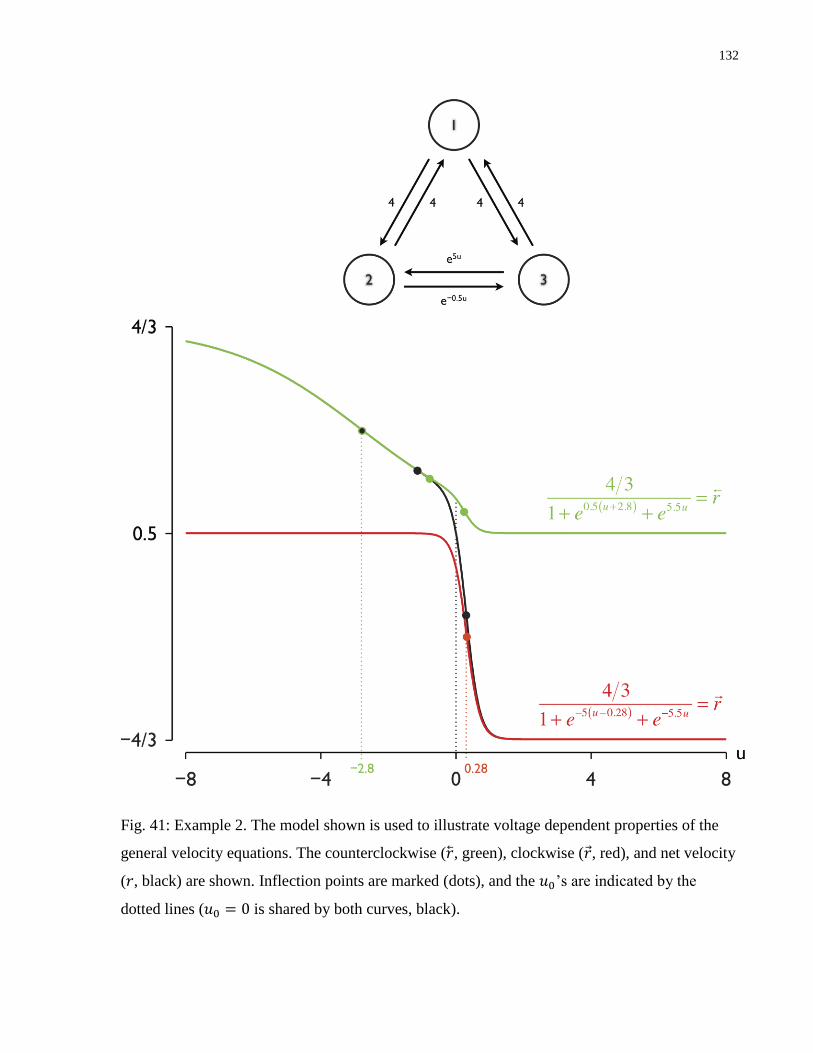
132
Fig. 41: Example 2. The model shown is used to illustrate voltage dependent properties of the
general velocity equations. The counterclockwise ( , green), clockwise ( , red), and net velocity
( , black) are shown. Inflection points are marked (dots), and the ’s are indicated by the
dotted lines ( is shared by both curves, black).

133
Fig. 42: Characteristics of the logarithmic exponential shifts. For a single binding event the ’s
can shift positive (blue) or negative (red). The red curve starts at infinity and asymptotically
approaches ( ) at large , while the blue starts at ( ) and increases to infinity. The
substrate concentrations where are indicated at the bottom.

134
Fig. 43: Example 3. Substrate dependence of the I–V curves. A substrate binding event is added
to two different steps of the model in Fig. 41, shown in the diagrams on the left; voltage
dependent transition in red, and substrate binding in blue. (A) Substrate dependence of the –
curves with overlaid paths showing ( ) (direction of the trajectories indicated by the
arrow). (B) – curves plotted on a log- scale with the bands shown in grey. curves
with a dependence are dashed, and are solid; those with increasing log
dependence are dark blue and a decreasing light blue. The equations are shown on the right.

135
Fig. 44: Analyzing experimental I–V data. (A) I–V substrate titration data were analyzed for the
Q170C mutant of rSGLT1 (1), hCNT3 (2)187, hSGLT1 (3)249 and rat NaPi-2 (4)197. These
curves were fit (black lines) with a one-term Boltzmann function, ( ( ))⁄ ;
in 1, is shared across Na+ concentrations, as expected for voltage dependent binding. The
fits returned ’s and ’s at each substrate concentration and they are plotted in B and C (axis tic
colours match data in A); ’s are also overlaid in A (open circle). (B) The valences were
mostly substrate independent and their average is indicated (dotted line). (C) The rising phase of
the – data at low was fit with the logarithmic function shown (blue), with results given on
the right (
). The intercept of this rising phase at zero can be calculated from and is
shown ( ( ) ( )⁄ , blue dotted line). A plateaued , from another term following a
downward or flat trajectory, would become dominant at high and was not fit as part of the
rising phase (red dotted line). The hCNT3 – data could not be fit, because the changing
valence indicated a changing dominant term.

136
Fig. 45: Steady-State velocity models. (B) The steady-state velocity equation was constructed
using the published turnover ( ) and apparent affinity ( ) data shown in A, and values for
and were calculated from the fit results in Fig. 44 using Eq. 25. It was found
that values calculated with gave better results than , and, therefore, these were used. (C)
The steady-state velocity equations in B are simulated (coloured lines). Turnover data for
Q170C rSGLT1188
, turnover12
and apparent affinity249
data for hSGLT1, and turnover and
affinity data for NaPi-2197
.
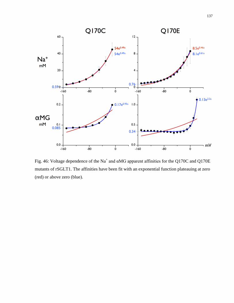
137
Fig. 46: Voltage dependence of the Na+ and αMG apparent affinities for the Q170C and Q170E
mutants of rSGLT1. The affinities have been fit with an exponential function plateauing at zero
(red) or above zero (blue).

138
Conclusion and Future Work 4
For a long time studying membrane transporters has been a block box analysis. Little was
known about their structure, let alone their inner workings, and the primary way to learn about
them was to stimulate and observe the output. Electrophysiological experiments have become
the pinnacle of these types of studies because of their unmatched ability to both stimulate and
observe. For many years, electrophysiological studies have uncovered curiosities and measured
parameters in greater detail, but without a physical representation of the carrier to work with it
was extremely difficult to unravel mechanisms with kinetic data alone. We are fortunate now to
have the structural data that we do from the crystal structures, as it provides a context for
interpreting kinetic data by essentially opening up the black box so we can gaze at its constituent
parts. Now that we can see how these biological machines are put together, kinetic studies are
more important than ever, as they provide a way to reverse engineer these proteins by observing
them in action. Kinetic and structural studies are complementary because they each fill in a
missing part of the other. It would be a mistake to assume that transporters can be understood by
looking only at their structures; a mistake on par with assuming that kinetics could do the same.
With that said, kinetic studies can only be helpful in elucidating mechanism, as opposed to a
tool for characterization, if we understand what the kinetic parameters measure. To do this we
need good models that can explain where the parameters come from, and accurate
measurements that provide authentic observations of the carrier. In this regard there are two
prominent time domains for kinetic studies, the transient and steady-state; equilibrium studies
could provide additional information, but they are less suited to electrophysiology and more so
for radioactive uptake. In this thesis we approached both time domains with a goal of
understanding the composition of their kinetics, and to then use this understanding to retrieve as
much kinetic information as possible. The hope was that by elucidating the nature of these
kinetics they could be related more easily back to an understanding of the carrier.
The transient project demonstrated that it was necessary to find all the decay components in
order to measure the kinetics of real conformational changes and not some form of weighted
average. When this was done it became much easier to interpret the kinetic data in terms of a
model, leading to a kinetic representation of the gated rocker-switch mechanism with its four

139
conformational changes. The steady-state project relied on theory to understand what factors
affect the cycling velocity. In this case we learned that the I–V curves are governed by rate
limiting patterns in the transport loop, and this led to new ways of measuring them, and a
method for building descriptive models from them. Most importantly, this allows us to think
about the transport loop in terms of these rate limiting patterns.
The transient and steady-state kinetics provide different windows into the carrier transport cycle.
Transient currents are mostly available only in the absence of the non-ionic substrate, and
therefore monitor conformational changes of the unloaded carrier (top of Fig. 31), while the
steady-state currents incorporate the entire transport loop, and are one of the few ways of
studying states in the presence of substrate. Although kinetics from transient studies are
theoretically superior because they provide information on individual conformational changes,
steady-state kinetics are necessary to study substrate binding. An ideal project would be to
combine transient and steady-state kinetic studies for a single carrier, such as SGLT1. The first
step would be to build a state model of the empty carrier conformations using transient kinetics
(top of Fig. 31). This model could then be used as a template for the carrier conformations in the
presence substrate (bottom of Fig. 31). Steady-state studies, in the forward and reverse
directions, could measure the kinetics of the various rate limiting patterns in each direction, and
the form and overlap of these patterns could be guessed at and incorporated into the model.
These techniques have introduced a number of kinetic parameters that can be used to
characterize and understand ion-coupled cotransporters. These provide new opportunities to
classify and compare cotransporters kinetically and study the effects of mutations. Using the
crystal structures as a guide, strategic mutations can be used to single out key parts of the
transport mechanism, while monitoring the effect kinetically with parameters that map onto
specific functions. As our understanding of the connection between these parameters and the
structure grows, these techniques will only become more effective. By understanding these
mechanisms we can better understand mutations that lead to disease, we can build better
inhibitors, and perhaps the ultimate goal is to one day build biological machines of our own.

140
References
1. Crane RK. The gradient hypothesis and other models of carrier-mediated active
transport. Rev Physiol Biochem Pharmacol. 1977;78:99–159.
2. Jardetzky O. Simple allosteric model for membrane pumps. Nature. 1966 Aug.
27;211(5052):969–970.
3. Schultz SG, Curran PF. Coupled transport of sodium and organic solutes. Physiol Rev.
1970 Oct.;50(4):637–718.
4. Kaback HR, Stadtman ER. Proline uptake by an isolated cytoplasmic membrane
preparation of Escherichia coli. Proc Natl Acad Sci USA. 1966 Apr.;55(4):920–927.
5. Hopfer U, Nelson K, Perrotto J, Isselbacher KJ. Glucose transport in isolated brush
border membrane from rat small intestine. J Biol Chem. 1973 Jan. 10;248(1):25–32.
6. Murer H, Kinne R. The use of isolated membrane vesicles to study epithelial transport
processes. J Membr Biol. 1980 Jul. 15;55(2):81–95.
7. Stevens BR, Kaunitz JD, Wright EM. Intestinal Transport of Amino Acids and Sugars:
Advances Using Membrane Vesicles. Annu Rev Physiol. Annual Reviews 4139 El
Camino Way, P.O. Box 10139, Palo Alto, CA 94303-0139, USA; 1984 Oct.;46(1):417–
433.
8. Silverman M. Structure and function of hexose transporters. Annu. Rev. Biochem.
1991;60:757–794.
9. Hediger MA, Coady MJ, Ikeda TS, Wright EM. Expression cloning and cDNA
sequencing of the Na+/glucose co-transporter. Nature. 1987;330(6146):379–381.
10. Wright EM, Hager KM, Turk E. Sodium cotransport proteins. Curr Opin Cell Biol.
1992 Aug. 1;4(4):696–702.
11. Hediger MA, Kanai Y, You G, Nussberger S. Mammalian ion-coupled solute
transporters. J Physiol (Lond). 1995 Jan.;482:7S–17S.
12. Longpré J-P, Lapointe J-Y. Determination of the Na+/glucose cotransporter (SGLT1)
turnover rate using the ion-trap technique. Biophys J. 2011 Jan. 5;100(1):52–59.
13. Bamberg E, Clarke RJ, Fendler K. Electrogenic properties of the Na+,K
+-ATPase
probed by presteady state and relaxation studies. J Bioenerg Biomembr. 2001 Oct.
1;33(5):401–405.
14. Doyle DA, Morais Cabral J, Pfuetzner RA, Kuo A, Gulbis JM, Cohen SL, et al. The
structure of the potassium channel: molecular basis of K+ conduction and selectivity.
Science. 1998 Apr. 3;280(5360):69–77.

141
15. Lo B, Silverman M. Cysteine scanning mutagenesis of the segment between putative
transmembrane helices IV and V of the high affinity Na+/Glucose cotransporter SGLT1.
Evidence that this region participates in the Na+ and voltage dependence of the
transporter. J Biol Chem. 1998 Nov. 6;273(45):29341–29351.
16. Liu T, Lo B, Speight P, Silverman M. Transmembrane IV of the high-affinity sodium-
glucose cotransporter participates in sugar binding. Am J Physiol, Cell Physiol. 2008
Jul.;295(1):C64–72.
17. Liu T, Speight P, Silverman M. Reanalysis of structure/function correlations in the
region of transmembrane segments 4 and 5 of the rabbit sodium/glucose cotransporter.
Biochem Biophys Res Commun. 2009 Jan. 2;378(1):133–138.
18. Loo DD, Hirayama BA, Gallardo EM, Lam JT, Turk E, Wright EM. Conformational
changes couple Na+ and glucose transport. Proc Natl Acad Sci USA. 1998 Jun.
23;95(13):7789–7794.
19. Gagnon DG, Bissonnette P, Lapointe J-Y. Identification of a disulfide bridge linking the
fourth and the seventh extracellular loops of the Na+/glucose cotransporter. J Gen
Physiol. 2006 Feb.;127(2):145–158.
20. Nagata T, Iizumi S, Satoh K, Kikuchi S. Comparative molecular biological analysis of
membrane transport genes in organisms. Plant Mol. Biol. 2008 Apr.;66(6):565–585.
21. Preston GM, Carroll TP, Guggino WB, Agre P. Appearance of water channels in
Xenopus oocytes expressing red cell CHIP28 protein. Science. 1992 Apr.
17;256(5055):385–387.
22. Murata K, Mitsuoka K, Hirai T, Walz T, Agre P, Heymann JB, et al. Structural
determinants of water permeation through aquaporin-1. Nature. 2000 Oct.
5;407(6804):599–605.
23. Carruthers A, DeZutter J, Ganguly A, Devaskar SU. Will the original glucose
transporter isoform please stand up! Am J Physiol Endocrinol Metab. 2009
Oct.;297(4):E836–48.
24. Abramson J, Smirnova I, Kasho V, Verner G, Kaback HR, Iwata S. Structure and
mechanism of the lactose permease of Escherichia coli. Science. 2003 Aug.
1;301(5633):610–615.
25. Toyoshima C, Nakasako M, Nomura H, Ogawa H. Crystal structure of the calcium
pump of sarcoplasmic reticulum at 2.6 A resolution. Nature. 2000 Jun.
8;405(6787):647–655.
26. Morth JP, Pedersen BP, Toustrup-Jensen MS, Sørensen TL-M, Petersen J, Andersen JP,
et al. Crystal structure of the sodium-potassium pump. Nature. 2007 Dec.
13;450(7172):1043–1049.
27. Pedersen BP, Buch-Pedersen MJ, Morth JP, Palmgren MG, Nissen P. Crystal structure

142
of the plasma membrane proton pump. Nature. 2007 Dec. 13;450(7172):1111–1114.
28. Morth JP, Pedersen BP, Buch-Pedersen MJ, Andersen JP, Vilsen B, Palmgren MG, et
al. A structural overview of the plasma membrane Na+,K
+-ATPase and H
+-ATPase ion
pumps. Nat Rev Mol Cell Biol. 2011 Jan.;12(1):60–70.
29. Grigorieff N, Ceska TA, Downing KH, Baldwin JM, Henderson R. Electron-
crystallographic refinement of the structure of bacteriorhodopsin. J Mol Biol. 1996 Jun.
14;259(3):393–421.
30. Hirai T, Heymann JAW, Shi D, Sarker R, Maloney PC, Subramaniam S. Three-
dimensional structure of a bacterial oxalate transporter. Nat Struct Biol. 2002 Jul.
15;9(8):597–600.
31. Huang Y, Lemieux MJ, Song J, Auer M, Wang D-N. Structure and mechanism of the
glycerol-3-phosphate transporter from Escherichia coli. Science. 2003 Aug.
1;301(5633):616–620.
32. Yin Y, He X, Szewczyk P, Nguyen T, Chang G. Structure of the multidrug transporter
EmrD from Escherichia coli. Science. 2006 May 5;312(5774):741–744.
33. Wright EM, Loo DDF, Hirayama BA, Turk E. Surprising versatility of Na+-glucose
cotransporters: SLC5. Physiology (Bethesda). 2004 Dec.;19:370–376.
34. Hediger MA, Romero MF, Peng J-B, Rolfs A, Takanaga H, Bruford EA. The ABCs of
solute carriers: physiological, pathological and therapeutic implications of human
membrane transport proteins. Pflugers Arch. 2004 Feb.;447(5):465–468.
35. Busch W, Saier MH. The transporter classification (TC) system, 2002. Crit Rev
Biochem Mol Biol. 2002;37(5):287–337.
36. Jung H. Towards the molecular mechanism of Na+/solute symport in prokaryotes.
Biochim Biophys Acta. 2001 May 1;1505(1):131–143.
37. Jung H. The sodium/substrate symporter family: structural and functional features.
FEBS Lett. 2002 Oct. 2;529(1):73–77.
38. Zhou L, Cryan EV, D'Andrea MR, Belkowski S, Conway BR, Demarest KT. Human
cardiomyocytes express high level of Na+/glucose cotransporter 1 (SGLT1). J Cell
Biochem. 2003 Oct. 1;90(2):339–346.
39. Banerjee SK, McGaffin KR, Pastor-Soler NM, Ahmad F. SGLT1 is a novel cardiac
glucose transporter that is perturbed in disease states. Cardiovasc Res. 2009 Oct.
1;84(1):111–118.
40. Wells RG, Pajor AM, Kanai Y, Turk E, Wright EM, Hediger MA. Cloning of a human
kidney cDNA with similarity to the sodium-glucose cotransporter. Am J Physiol. 1992
Sep.;263(3 Pt 2):F459–65.

143
41. Kanai Y, Lee WS, You G, Brown D, Hediger MA. The human kidney low affinity
Na+/glucose cotransporter SGLT2. Delineation of the major renal reabsorptive
mechanism for D-glucose. J Clin Invest. 1994;93(1):397–404.
42. Chen XZ, Coady MJ, Jackson F, Berteloot A, Lapointe JY. Thermodynamic
determination of the Na+: glucose coupling ratio for the human SGLT1 cotransporter.
Biophys J. 1995 Dec. 1;69(6):2405–2414.
43. Wright EM, Turk E, Martín MG. Molecular basis for glucose-galactose malabsorption.
Cell Biochem. Biophys. 2002;36(2-3):115–121.
44. Wright EM, Martín MG, Turk E. Intestinal absorption in health and disease--sugars.
Best Pract Res Clin Gastroenterol. 2003 Dec.;17(6):943–956.
45. Santer R, Kinner M, Lassen CL, Schneppenheim R, Eggert P, Bald M, et al. Molecular
analysis of the SGLT2 gene in patients with renal glucosuria. J Am Soc Nephrol. 2003
Nov. 1;14(11):2873–2882.
46. Calado J, Sznajer Y, Metzger D, Rita A, Hogan MC, Kattamis A, et al. Twenty-one
additional cases of familial renal glucosuria: absence of genetic heterogeneity, high
prevalence of private mutations and further evidence of volume depletion. Nephrol Dial
Transplant. 2008 Dec. 1;23(12):3874–3879.
47. Calado J, Loeffler J, Sakallioglu O, Gok F, Lhotta K, Barata J, et al. Familial renal
glucosuria: SLC5A2 mutation analysis and evidence of salt-wasting. Kidney Int. 2006
Mar.;69(5):852–855.
48. Magen D, Sprecher E, Zelikovic I, Skorecki K. A novel missense mutation in SLC5A2
encoding SGLT2 underlies autosomal-recessive renal glucosuria and aminoaciduria.
Kidney Int. 2005;67(1):34–41.
49. Francis J, Zhang J, Farhi A, Carey H, Geller DS. A novel SGLT2 mutation in a patient
with autosomal recessive renal glucosuria. Nephrol. Dial. Transplant. 2004
Nov.;19(11):2893–2895.
50. Kleta R, Stuart C, Gill FA, Gahl WA. Renal glucosuria due to SGLT2 mutations. Mol
Genet Metab. 2004 May;82(1):56–58.
51. Calado J, Soto K, Clemente C, Correia P, Rueff J. Novel compound heterozygous
mutations in SLC5A2 are responsible for autosomal recessive renal glucosuria. Hum.
Genet. 2004 Feb.;114(3):314–316.
52. den Heuvel van LP, Assink K, Willemsen M, Monnens L. Autosomal recessive renal
glucosuria attributable to a mutation in the sodium glucose cotransporter (SGLT2).
Hum Genet. 2002 Dec. 1;111(6):544–547.
53. Cho B-S, Kim S-D. School urinalysis screening in Korea. Nephrology (Carlton). 2007
Dec. 1;12 Suppl 3:S3–7.
144
54. Katsuno K, Fujimori Y, Takemura Y, Hiratochi M, Itoh F, Komatsu Y, et al.
Sergliflozin, a novel selective inhibitor of low-affinity sodium glucose cotransporter
(SGLT2), validates the critical role of SGLT2 in renal glucose reabsorption and
modulates plasma glucose level. J Pharmacol Exp Ther. 2007;320(1):323–330.
55. Meng W, Ellsworth BA, Nirschl AA, McCann PJ, Patel M, Girotra RN, et al. Discovery
of dapagliflozin: a potent, selective renal sodium-dependent glucose cotransporter 2
(SGLT2) inhibitor for the treatment of type 2 diabetes. J Med Chem. 2008 Mar.
13;51(5):1145–1149.
56. Hussey EK, Clark RV, Amin DM, Kipnes MS, O'Connor-Semmes RL, O'Driscoll EC,
et al. Single-dose pharmacokinetics and pharmacodynamics of sergliflozin etabonate, a
novel inhibitor of glucose reabsorption, in healthy volunteers and patients with type 2
diabetes mellitus. J Clin Pharmacol. 2010 Jun. 1;50(6):623–635.
57. Hussey EK, Dobbins RL, Stoltz RR, Stockman NL, O'Connor-Semmes RL, Kapur A, et
al. Multiple-dose pharmacokinetics and pharmacodynamics of sergliflozin etabonate, a
novel inhibitor of glucose reabsorption, in healthy overweight and obese subjects: a
randomized double-blind study. J Clin Pharmacol. 2010 Jun. 1;50(6):636–646.
58. Marsenic O. Glucose control by the kidney: an emerging target in diabetes. Am J
Kidney Dis. 2009 May 1;53(5):875–883.
59. Trial watch: SGLT2 inhibitor shows promise in type 2 diabetes. Nat Rev Drug Discov.
2010 Mar.;:182.
60. Kong CT, Yet SF, Lever JE. Cloning and expression of a mammalian Na+/amino acid
cotransporter with sequence similarity to Na+/glucose cotransporters. J Biol Chem. 1993
Jan. 25;268(3):1509–1512.
61. Mackenzie B, Panayotova-Heiermann M, Loo DD, Lever JE, Wright EM. SAATl Is a
Low Affinity Na+/ Glucose Cotransporter and Not an Amino Acid Transporter. J Biol
Chem. 1994 Sep. p. 22488–22491.
62. Mackenzie B, Loo DD, Panayotova-Heiermann M, Wright EM. Biophysical
characteristics of the pig kidney Na+/glucose cotransporter SGLT2 reveal a common
mechanism for SGLT1 and SGLT2. J Biol Chem. 1996 Dec. 20;271(51):32678–32683.
63. Díez-Sampedro A, Lostao MP, Wright EM, Hirayama BA. Glycoside binding and
translocation in Na+-dependent glucose cotransporters: comparison of SGLT1 and
SGLT3. J Membr Biol. 2000 Jul. 15;176(2):111–117.
64. Díez-Sampedro A, Eskandari S, Wright EM, Hirayama BA. Na+-to-sugar stoichiometry
of SGLT3. Am J Physiol Renal Physiol. 2001 Feb. 1;280(2):F278–82.
65. Voss AA, Díez-Sampedro A, Hirayama BA, Loo DDF, Wright EM. Imino sugars are
potent agonists of the human glucose sensor SGLT3. Mol Pharmacol. 2007 Feb.
1;71(2):628–634.

145
66. Diez-Sampedro A, Hirayama BA, Osswald C, Gorboulev V, Baumgarten K, Volk C, et
al. A glucose sensor hiding in a family of transporters. Proc Natl Acad Sci USA. 2003
Sep. 30;100(20):11753–11758.
67. Bianchi L, Díez-Sampedro A. A single amino acid change converts the sugar sensor
SGLT3 into a sugar transporter. PLoS ONE. 2010;5(4):e10241.
68. Faham S, Watanabe A, Besserer GM, Cascio D, Specht A, Hirayama BA, et al. The
crystal structure of a sodium galactose transporter reveals mechanistic insights into
Na+/sugar symport. Science. 2008 Aug. 8;321(5890):810–814.
69. Tazawa S, Yamato T, Fujikura H, Hiratochi M, Itoh F, Tomae M, et al.
SLC5A9/SGLT4, a new Na+-dependent glucose transporter, is an essential transporter
for mannose, 1,5-anhydro-D-glucitol, and fructose. Life Sci. 2005 Jan. 14;76(9):1039–
1050.
70. Parent L, Supplisson S, Loo DD, Wright EM. Electrogenic properties of the cloned
Na+/glucose cotransporter: II. A transport model under nonrapid equilibrium conditions.
J Membr Biol. 1992;125(1):63–79.
71. Wright EM, Hirayama BA, Loo DF. Active sugar transport in health and disease. J.
Intern. Med. 2007 Jan.;261(1):32–43.
72. Moran A, Davis LJ, Turner RJ. High affinity phlorizin binding to the LLC-PK1 cells
exhibits a sodium:phlorizin stoichiometry of 2:1. J Biol Chem. 1988 Jan. 5;263(1):187–
192.
73. Chen XZ, Coady MJ, Jalal F, Wallendorff B, Lapointe JY. Sodium leak pathway and
substrate binding order in the Na+-glucose cotransporter. Biophys J. 1997 Nov.
1;73(5):2503–2510.
74. Oulianova N, Falk S, Berteloot A. Two-step mechanism of phlorizin binding to the
SGLT1 protein in the kidney. J Membr Biol. 2001 Feb. 1;179(3):223–242.
75. Kimmich GA. Membrane potentials and the mechanism of intestinal Na+-dependent
sugar transport. J Membr Biol. 1990 Mar.;114(1):1–27.
76. Berteloot A. Kinetic Mechanism of Na+ -Glucose Cotransport through the Rabbit
Intestinal SGLT1 Protein. Journal of Membrane Biology. 2003 Apr. 1;192(2):89–100.
77. Gagnon DG, Frindel C, Lapointe J-Y. Effect of substrate on the pre-steady-state
kinetics of the Na+/glucose cotransporter. Biophys J. 2007 Jan. 15;92(2):461–472.
78. Longpré J-P, Gagnon DG, Coady MJ, Lapointe J-Y. The actual ionic nature of the leak
current through the Na+/glucose cotransporter SGLT1. Biophys J. 2010 Jan.
20;98(2):231–239.
79. Charron FM, Blanchard MG, Lapointe J-Y. Intracellular hypertonicity is responsible for
water flux associated with Na+/glucose cotransport. Biophys J. 2006 May

146
15;90(10):3546–3554.
80. Sauer GA, Nagel G, Koepsell H, Bamberg E, Hartung K. Voltage and substrate
dependence of the inverse transport mode of the rabbit Na+/glucose cotransporter
(SGLT1). FEBS Lett. 2000 Mar. 3;469(1):98–100.
81. Quick M, Tomasevic J, Wright EM. Functional asymmetry of the human Na+/glucose
transporter (hSGLT1) in bacterial membrane vesicles. Biochemistry. 2003 Aug.
5;42(30):9147–9152.
82. Eskandari S, Wright EM, Loo DDF. Kinetics of the reverse mode of the Na+/glucose
cotransporter. J Membr Biol. 2005 Mar.;204(1):23–32.
83. Loo DD, Hazama A, Supplisson S, Turk E, Wright EM. Relaxation kinetics of the
Na+/glucose cotransporter. Proc Natl Acad Sci USA. 1993 Jun. 15;90(12):5767–5771.
84. Loo DDF, Hirayama BA, Cha A, Bezanilla F, Wright EM. Perturbation analysis of the
voltage-sensitive conformational changes of the Na+/glucose cotransporter. J Gen
Physiol. 2005 Jan.;125(1):13–36.
85. Chen XZ, Coady MJ, Lapointe JY. Fast voltage clamp discloses a new component of
presteady-state currents from the Na+-glucose cotransporter. Biophys J. 1996 Nov.
1;71(5):2544–2552.
86. Krofchick D, Silverman M. Investigating the conformational states of the rabbit
Na+/glucose cotransporter. Biophys J. 2003 Jun.;84(6):3690–3702.
87. Kwon HM, Yamauchi A, Uchida S, Preston AS, Garcia-Perez A, Burg MB, et al.
Cloning of the cDNa for a Na+/myo-inositol cotransporter, a hypertonicity stress
protein. J Biol Chem. 1992 Mar. 25;267(9):6297–6301.
88. Hitomi K, Tsukagoshi N. cDNA sequence for rkST1, a novel member of the sodium
ion-dependent glucose cotransporter family. Biochim Biophys Acta. 1994 Mar.
23;1190(2):469–472.
89. Roll P, Massacrier A, Pereira S, Robaglia-Schlupp A, Cau P, Szepetowski P. New
human sodium/glucose cotransporter gene (KST1): identification, characterization, and
mutation analysis in ICCA (infantile convulsions and choreoathetosis) and BFIC
(benign familial infantile convulsions) families. Gene. 2002 Feb. 20;285(1-2):141–148.
90. Beck FX, Schmolke M, Guder WG. Osmolytes. Curr Opin Nephrol Hypertens. 1992
Oct. 1;1(1):43–52.
91. York JD, Guo S, Odom AR, Spiegelberg BD, Stolz LE. An expanded view of inositol
signaling. Adv Enzyme Regul. 2001;41:57–71.
92. Levine J, Barak Y, Gonzalves M, Szor H, Elizur A, Kofman O, et al. Double-blind,
controlled trial of inositol treatment of depression. AJP. American Psychiatric
Association; 1995 May 1;152(5):792–794.

147
93. Benjamin J, Levine J, Fux M, Aviv A, Levy D, Belmaker R. Double-blind, placebo-
controlled, crossover trial of inositol treatment for panic disorder. AJP. American
Psychiatric Association; 1995 Jul. 1;152(7):1084–1086.
94. Fux M, Levine J, Aviv A, Belmaker RH. Inositol treatment of obsessive-compulsive
disorder. Am J Psychiatry. 1996 Sep.;153(9):1219–1221.
95. Nestler JE, Jakubowicz DJ, Reamer P, Gunn RD, Allan G. Ovulatory and metabolic
effects of D-chiro-inositol in the polycystic ovary syndrome. N. Engl. J. Med. 1999
Apr. 29;340(17):1314–1320.
96. Berry GT, Mallee JJ, Kwon HM, Rim JS, Mulla WR, Muenke M, et al. The human
osmoregulatory Na+/myo-inositol cotransporter gene (SLC5A3): molecular cloning and
localization to chromosome 21. Genomics. 1995 Jan. 20;25(2):507–513.
97. Poppe R, Karbach U, Gambaryan S, Wiesinger H, Lutzenburg M, Kraemer M, et al.
Expression of the Na+ D Glucose Cotransporter SGLT1 in Neurons. J Neurochem.
1997;69:84–94.
98. Lahjouji K, Aouameur R, Bissonnette P, Coady MJ, Bichet DG, Lapointe J-Y.
Expression and functionality of the Na+/myo-inositol cotransporter SMIT2 in rabbit
kidney. Biochim Biophys Acta. 2007 May 1;1768(5):1154–1159.
99. Aouameur R, Da Cal S, Bissonnette P, Coady MJ, Lapointe J-Y. SMIT2 mediates all
myo-inositol uptake in apical membranes of rat small intestine. Am J Physiol
Gastrointest Liver Physiol. 2007 Dec.;293(6):G1300–7.
100. Berry GT, Wu S, Buccafusca R, Ren J, Gonzales LW, Ballard PL, et al. Loss of murine
Na+/myo-inositol cotransporter leads to brain myo-inositol depletion and central apnea.
J Biol Chem. 2003 May 16;278(20):18297–18302.
101. Chau JFL, Lee MK, Law JWS, Chung SK, Chung SSM. Sodium/myo-inositol
cotransporter-1 is essential for the development and function of the peripheral nerves.
FASEB J. 2005 Nov. 1;19(13):1887–1889.
102. Berry GT, Wang ZJ, Dreha SF, Finucane BM, Zimmerman RA. In vivo brain myo-
inositol levels in children with Down syndrome. J Pediatr. Elsevier; 1999 Jul.
1;135(1):94–97.
103. Willmroth F, Drieling T, Lamla U, Marcushen M, Wark H-J, van Calker D. Sodium-
myo-inositol co-transporter (SMIT-1) mRNA is increased in neutrophils of patients with
bipolar 1 disorder and down-regulated under treatment with mood stabilizers. Int J
Neuropsychopharmacol. 2007 Feb. 1;10(1):63–71.
104. van Calker D, Belmaker RH. The high affinity inositol transport system--implications
for the pathophysiology and treatment of bipolar disorder. Bipolar Disord. 2000 Jun.
1;2(2):102–107.
105. Coady MJ, Wallendorff B, Gagnon DG, Lapointe J-Y. Identification of a novel

148
Na+/myo-inositol cotransporter. J Biol Chem. 2002 Sep. 20;277(38):35219–35224.
106. Bourgeois F, Coady MJ, Lapointe J-Y. Determination of transport stoichiometry for two
cation-coupled myo-inositol cotransporters: SMIT2 and HMIT. J Physiol (Lond). 2005
Mar. 1;563(Pt 2):333–343.
107. Hager K, Hazama A, Kwon HM, Loo DD, Handler JS, Wright EM. Kinetics and
specificity of the renal Na+/myo-inositol cotransporter expressed in Xenopus oocytes. J
Membr Biol. 1995;143(2):103–113.
108. Ganapathy V, Thangaraju M, Gopal E, Martin PM, Itagaki S, Miyauchi S, et al.
Sodium-coupled monocarboxylate transporters in normal tissues and in cancer. AAPS J.
2008;10(1):193–199.
109. Miyauchi S, Gopal E, Fei Y-J, Ganapathy V. Functional identification of SLC5A8, a
tumor suppressor down-regulated in colon cancer, as a Na+-coupled transporter for
short-chain fatty acids. J Biol Chem. 2004 Apr. 2;279(14):13293–13296.
110. Coady MJ, Chang M-H, Charron FM, Plata C, Wallendorff B, Sah JF, et al. The human
tumour suppressor gene SLC5A8 expresses a Na+-monocarboxylate cotransporter. J
Physiol (Lond). 2004 Jun. 15;557(Pt 3):719–731.
111. Coady MJ, Wallendorff B, Bourgeois F, Charron F, Lapointe J-Y. Establishing a
definitive stoichiometry for the Na+/monocarboxylate cotransporter SMCT1. Biophys J.
2007 Oct. 1;93(7):2325–2331.
112. Srinivas SR, Gopal E, Zhuang L, Itagaki S, Martin PM, Fei Y-J, et al. Cloning and
functional identification of slc5a12 as a sodium-coupled low-affinity transporter for
monocarboxylates (SMCT2). Biochem J. 2005 Dec. 15;392(Pt 3):655–664.
113. Gopal E, Umapathy NS, Martin PM, Ananth S, Gnana-Prakasam JP, Becker H, et al.
Cloning and functional characterization of human SMCT2 (SLC5A12) and expression
pattern of the transporter in kidney. Biochim Biophys Acta. 2007 Nov.;1768(11):2690–
2697.
114. Plata C, Sussman CR, Sindic A, Liang JO, Mount DB, Josephs ZM, et al. Zebrafish
Slc5a12 encodes an electroneutral sodium monocarboxylate transporter (SMCTn). A
comparison with the electrogenic SMCT (SMCTe/Slc5a8). J Biol Chem. 2007 Apr.
20;282(16):11996–12009.
115. Wright EM, Turk E. The sodium/glucose cotransport family SLC5. Pflugers Arch. 2004
Feb.;447(5):510–518.
116. Coady MJ, Wallendorff B, Bourgeois F, Lapointe J-Y. Anionic leak currents through
the Na+/monocarboxylate cotransporter SMCT1. Am J Physiol, Cell Physiol. 2010
Jan.;298(1):C124–31.
117. Rodriguez A-M, Perron B, Lacroix L, Caillou B, Leblanc G, Schlumberger M, et al.
Identification and characterization of a putative human iodide transporter located at the

149
apical membrane of thyrocytes. J Clin Endocrinol Metab. 2002 Jul. 1;87(7):3500–3503.
118. Gopal E, Fei Y-J, Sugawara M, Miyauchi S, Zhuang L, Martin P, et al. Expression of
slc5a8 in kidney and its role in Na+-coupled transport of lactate. J Biol Chem. 2004 Oct.
22;279(43):44522–44532.
119. Frank H, Gröger N, Diener M, Becker C, Braun T, Boettger T. Lactaturia and loss of
sodium-dependent lactate uptake in the colon of SLC5A8-deficient mice. J Biol Chem.
2008 Sep. 5;283(36):24729–24737.
120. Li H, Myeroff L, Smiraglia D, Romero MF, Pretlow TP, Kasturi L, et al. SLC5A8, a
sodium transporter, is a tumor suppressor gene silenced by methylation in human colon
aberrant crypt foci and cancers. Proc Natl Acad Sci USA. 2003 Jul. 8;100(14):8412–
8417.
121. Ganapathy V, Gopal E, Miyauchi S, Prasad PD. Biological functions of SLC5A8, a
candidate tumour suppressor. Biochem Soc Trans. 2005 Feb. 1;33(Pt 1):237–240.
122. Thangaraju M, Gopal E, Martin PM, Ananth S, Smith SB, Prasad PD, et al. SLC5A8
triggers tumor cell apoptosis through pyruvate-dependent inhibition of histone
deacetylases. Cancer Res. 2006 Dec. 15;66(24):11560–11564.
123. Gupta N, Martin PM, Prasad PD, Ganapathy V. SLC5A8 (SMCT1)-mediated transport
of butyrate forms the basis for the tumor suppressive function of the transporter. Life
Sci. 2006 Apr. 18;78(21):2419–2425.
124. Iwamoto H, Blakely RD, De Felice LJ. Na+, Cl
−, and pH dependence of the human
choline transporter (hCHT) in Xenopus oocytes: the proton inactivation hypothesis of
hCHT in synaptic vesicles. J Neurosci. 2006 Sep. 27;26(39):9851–9859.
125. Okuda T, Haga T, Kanai Y, Endou H, Ishihara T, Katsura I. Identification and
characterization of the high-affinity choline transporter. Nat Neurosci. 2000 Feb.
1;3(2):120–125.
126. Ferguson SM, Savchenko V, Apparsundaram S, Zwick M, Wright J, Heilman CJ, et al.
Vesicular localization and activity-dependent trafficking of presynaptic choline
transporters. J Neurosci. 2003 Oct. 29;23(30):9697–9709.
127. Ferguson SM, Blakely RD. The choline transporter resurfaces: new roles for synaptic
vesicles? Mol Interv. 2004 Feb. 1;4(1):22–37.
128. Okuda T, Haga T. Functional characterization of the human high-affinity choline
transporter. FEBS Lett. 2000 Nov. 3;484(2):92–97.
129. Apparsundaram S, Ferguson SM, George AL, Blakely RD. Molecular cloning of a
human, hemicholinium-3-sensitive choline transporter. Biochem Biophys Res
Commun. 2000 Oct. 5;276(3):862–867.
130. Smanik PA, Liu Q, Furminger TL, Ryu K, Xing S, Mazzaferri EL, et al. Cloning of the

150
human sodium lodide symporter. Biochem Biophys Res Commun. 1996 Sep.
13;226(2):339–345.
131. Riedel C, Dohán O, la Vieja De A, Ginter CS, Carrasco N. Journey of the iodide
transporter NIS: from its molecular identification to its clinical role in cancer. Trends
Biochem Sci. 2001 Aug. 1;26(8):490–496.
132. Dohán O, la Vieja De A, Paroder V, Riedel C, Artani M, Reed M, et al. The
sodium/iodide Symporter (NIS): characterization, regulation, and medical significance.
Endocr Rev. 2003 Feb. 1;24(1):48–77.
133. Eskandari S, Loo DD, Dai G, Levy O, Wright EM, Carrasco N. Thyroid Na+/I
-
symporter. Mechanism, stoichiometry, and specificity. J Biol Chem. 1997 Oct.
24;272(43):27230–27238.
134. Levy O, Ginter CS, la Vieja De A, Levy D, Carrasco N. Identification of a structural
requirement for thyroid Na+/I
− symporter (NIS) function from analysis of a mutation
that causes human congenital hypothyroidism. FEBS Lett. 1998 Jun. 5;429(1):36–40.
135. Prasad PD, Wang H, Kekuda R, Fujita T, Fei YJ, Devoe LD, et al. Cloning and
functional expression of a cDNA encoding a mammalian sodium-dependent vitamin
transporter mediating the uptake of pantothenate, biotin, and lipoate. J Biol Chem. 1998
Mar. 27;273(13):7501–7506.
136. Wang H, Huang W, Fei YJ, Xia H, Yang-Feng TL, Leibach FH, et al. Human placental
Na+-dependent multivitamin transporter. Cloning, functional expression, gene structure,
and chromosomal localization. J Biol Chem. 1999 May 21;274(21):14875–14883.
137. Balamurugan K, Ortiz A, Said HM. Biotin uptake by human intestinal and liver
epithelial cells: role of the SMVT system. Am J Physiol Gastrointest Liver Physiol.
2003 Jul. 1;285(1):G73–7.
138. Pajor AM. Sequence of a putative transporter from rabbit kidney related to the
Na+/glucose cotransporter gene family. Biochim Biophys Acta. 1994 Sep.
14;1194(2):349–351.
139. Zhao F-Q, Zheng Y-C, Wall EH, McFadden TB. Cloning and expression of bovine
sodium/glucose cotransporters. J. Dairy Sci. 2005 Jan.;88(1):182–194.
140. Gilbert ER, Li H, Emmerson DA, Webb KE, Wong EA. Developmental regulation of
nutrient transporter and enzyme mRNA abundance in the small intestine of broilers.
Poult Sci. 2007 Aug. 1;86(8):1739–1753.
141. Xie Z, Turk E, Wright EM. Characterization of the Vibrio parahaemolyticus
Na+/Glucose cotransporter. A bacterial member of the sodium/glucose transporter
(SGLT) family. J Biol Chem. 2000 Aug. 25;275(34):25959–25964.
142. Leung DW, Turk E, Kim O, Wright EM. Functional expression of the Vibrio
parahaemolyticus Na+/galactose (vSGLT) cotransporter in Xenopus laevis oocytes. J

151
Membr Biol. 2002 May 1;187(1):65–70.
143. Hediger MA, Turk E, Wright EM. Homology of the human intestinal Na+/glucose and
Escherichia coli Na+/proline cotransporters. Proc Natl Acad Sci USA. 1989
Aug.;86(15):5748–5752.
144. Schwan WR, Coulter SN, Ng EY, Langhorne MH, Ritchie HD, Brody LL, et al.
Identification and characterization of the PutP proline permease that contributes to in
vivo survival of Staphylococcus aureus in animal models. Infect Immun. 1998 Feb.
1;66(2):567–572.
145. Bayer AS, Coulter SN, Stover CK, Schwan WR. Impact of the high-affinity proline
permease gene (putP) on the virulence of Staphylococcus aureus in experimental
endocarditis. Infect Immun. 1999 Feb. 1;67(2):740–744.
146. Olkhova E, Raba M, Bracher S, Hilger D, Jung H. Homology model of the Na+/proline
transporter PutP of Escherichia coli and its functional implications. J. Mol. Biol. 2011
Feb. 11;406(1):59–74.
147. Jackowski S, Alix JH. Cloning, sequence, and expression of the pantothenate permease
(panF) gene of Escherichia coli. J. Bacteriol. 1990 Jul.;172(7):3842–3848.
148. Reizer J, Reizer A, Saier MH. The Na+/pantothenate symporter (PanF) of Escherichia
coli is homologous to the Na+/proline symporter (PutP) of E. coli and the Na
+/glucose
symporters of mammals. Res Microbiol. 1990 Oct.;141(9):1069–1072.
149. Murakami S, Nakashima R, Yamashita E, Yamaguchi A. Crystal structure of bacterial
multidrug efflux transporter AcrB. Nature. 2002 Oct. 10;419(6907):587–593.
150. Chen Y-J, Pornillos O, Lieu S, Ma C, Chen AP, Chang G. X-ray structure of EmrE
supports dual topology model. Proc Natl Acad Sci USA. 2007 Nov. 27;104(48):18999–
19004.
151. Bowie JU. Flip-flopping membrane proteins. Nat Struct Mol Biol. 2006 Feb. 1;:94–96.
152. Rapp M, Seppälä S, Granseth E, Heijne von G. Emulating membrane protein evolution
by rational design. Science. 2007 Mar. 2;315(5816):1282–1284.
153. Yamashita A, Singh SK, Kawate T, Jin Y, Gouaux E. Crystal structure of a bacterial
homologue of Na+/Cl
−-dependent neurotransmitter transporters. Nature. 2005 Sep.
8;437(7056):215–223.
154. Weyand S, Shimamura T, Yajima S, Suzuki S, Mirza O, Krusong K, et al. Structure and
molecular mechanism of a nucleobase-cation-symport-1 family transporter. Science.
2008 Oct. 31;322(5902):709–713.
155. Ressl S, Terwisscha van Scheltinga AC, Vonrhein C, Ott V, Ziegler C. Molecular basis
of transport and regulation in the Na+/betaine symporter BetP. Nature. 2009 Mar.
5;458(7234):47–52.

152
156. Gao X, Lu F, Zhou L, Dang S, Sun L, Li X, et al. Structure and mechanism of an amino
acid antiporter. Science. 2009 Jun. 19;324(5934):1565–1568.
157. Fang Y, Jayaram H, Shane T, Kolmakova-Partensky L, Wu F, Williams C, et al.
Structure of a prokaryotic virtual proton pump at 3.2 Å resolution. Nature. 2009 Aug.
20;460(7258):1040–1043.
158. Shaffer PL, Goehring A, Shankaranarayanan A, Gouaux E. Structure and mechanism of
a Na+-independent amino acid transporter. Science. 2009 Aug. 21;325(5943):1010–
1014.
159. Tang L, Bai L, Wang W-H, Jiang T. Crystal structure of the carnitine transporter and
insights into the antiport mechanism. Nat Struct Mol Biol. 2010 Apr. 1;17(4):492–496.
160. Sennhauser G, Bukowska MA, Briand C, Grütter MG. Crystal structure of the
multidrug exporter MexB from Pseudomonas aeruginosa. J Mol Biol. 2009 May
29;389(1):134–145.
161. Hunte C, Screpanti E, Venturi M, Rimon A, Padan E, Michel H. Structure of a Na+/H
+
antiporter and insights into mechanism of action and regulation by pH. Nature. Nature
Publishing Group; 2005 Jun. 30;435(7046):1197–1202.
162. Yernool D, Boudker O, Jin Y, Gouaux E. Structure of a glutamate transporter
homologue from Pyrococcus horikoshii. Nature. 2004 Oct. 14;431(7010):811–818.
163. Singh SK, Piscitelli CL, Yamashita A, Gouaux E. A competitive inhibitor traps LeuT in
an open-to-out conformation. Science. 2008 Dec. 12;322(5908):1655–1661.
164. Singh SK, Yamashita A, Gouaux E. Antidepressant binding site in a bacterial
homologue of neurotransmitter transporters. Nature. 2007 Aug. 23;448(7156):952–956.
165. Zhou Z, Zhen J, Karpowich NK, Goetz RM, Law CJ, Reith MEA, et al. LeuT-
desipramine structure reveals how antidepressants block neurotransmitter reuptake.
Science. 2007 Sep. 7;317(5843):1390–1393.
166. Lolkema JS, Slotboom D-J. The major amino acid transporter superfamily has a similar
core structure as Na+-galactose and Na
+-leucine transporters. Mol Membr Biol. 2008
Sep.;25(6-7):567–570.
167. Gao X, Zhou L, Jiao X, Lu F, Yan C, Zeng X, et al. Mechanism of substrate recognition
and transport by an amino acid antiporter. Nature. 2010 Feb. 11;463(7282):828–832.
168. Abramson J, Wright EM. Structure and function of Na+-symporters with inverted
repeats. Curr Opin Struct Biol. 2009 Aug. 1;19(4):425–432.
169. Sujatha MS, Balaji PV. Identification of common structural features of binding sites in
galactose-specific proteins. Proteins. 2004 Apr. 1;55(1):44–65.
170. Walle T, Walle UK. The beta-D-glucoside and sodium-dependent glucose transporter 1
153
(SGLT1)-inhibitor phloridzin is transported by both SGLT1 and multidrug resistance-
associated proteins 1/2. Drug Metab Dispos. 2003 Nov. 1;31(11):1288–1291.
171. Panayotova-Heiermann M, Loo DD, Kong CT, Lever JE, Wright EM. Sugar binding to
Na+/glucose cotransporters is determined by the carboxyl-terminal half of the protein. J
Biol Chem. 1996 Apr. 26;271(17):10029–10034.
172. Shaffer PL, Goehring A, Shankaranarayanan A, Gouaux E. SOM: Structure and
mechanism of a Na+-independent amino acid transporter. Science. 2009 Aug.
21;325(5943):1010–1014.
173. Diallinas G. Biochemistry. An almost-complete movie. Science. 2008 Dec.
12;322(5908):1644–1645.
174. Parent L, Supplisson S, Loo DD, Wright EM. Electrogenic properties of the cloned
Na+/glucose cotransporter: I. Voltage-clamp studies. J Membr Biol. 1992;125(1):49–62.
175. Loo DDF, Hirayama BA, Sala-Rabanal M, Wright EM. How drugs interact with
transporters: SGLT1 as a model. J Membr Biol. 2008 May 1;223(2):87–106.
176. Hilgemann DW. Channel-like function of the Na,K pump probed at microsecond
resolution in giant membrane patches. Science. 1994 Mar. 11;263(5152):1429–1432.
177. Holmgren M, Wagg J, Bezanilla F, Rakowski RF, De Weer P, Gadsby DC. Three
distinct and sequential steps in the release of sodium ions by the Na+/K
+-ATPase.
Nature. 2000 Feb. 24;403(6772):898–901.
178. Hirayama BA, Díez-Sampedro A, Wright EM. Common mechanisms of inhibition for
the Na+/glucose (hSGLT1) and Na
+/Cl
−/GABA (hGAT1) cotransporters. Br J
Pharmacol. 2001 Oct. 1;134(3):484–495.
179. Panayotova-Heiermann M, Loo DD, Lostao MP, Wright EM. Sodium/D-glucose
cotransporter charge movements involve polar residues. J Biol Chem. 1994 Aug.
19;269(33):21016–21020.
180. Mager S, Naeve J, Quick M, Labarca C, Davidson N, Lester HA. Steady states, charge
movements, and rates for a cloned GABA transporter expressed in Xenopus oocytes.
Neuron. 1993 Feb.;10(2):177–188.
181. Mager S, Min C, Henry DJ, Chavkin C, Hoffman BJ, Davidson N, et al. Conducting
states of a mammalian serotonin transporter. Neuron. 1994 Apr.;12(4):845–859.
182. Wadiche JI, Arriza JL, Amara SG, Kavanaugh MP. Kinetics of a human glutamate
transporter. Neuron. 1995 May;14(5):1019–1027.
183. Boorer KJ, Loo DD, Wright EM. Steady-state and presteady-state kinetics of the
H+/hexose cotransporter (STP1) from Arabidopsis thaliana expressed in Xenopus
oocytes. J Biol Chem. 1994 Aug. 12;269(32):20417–20424.

154
184. Mackenzie B, Loo DD, Fei Y, Liu WJ, Ganapathy V, Leibach FH, et al. Mechanisms of
the human intestinal H+-coupled oligopeptide transporter hPEPT1. J Biol Chem. 1996
Mar. 8;271(10):5430–5437.
185. Taglialatela M, Toro L, Stefani E. Novel voltage clamp to record small, fast currents
from ion channels expressed in Xenopus oocytes. Biophys J. 1992 Jan.;61(1):78–82.
186. Meinild A-K, Hirayama BA, Wright EM, Loo DDF. Fluorescence studies of ligand-
induced conformational changes of the Na+/glucose cotransporter. Biochemistry. 2002
Jan. 29;41(4):1250–1258.
187. Gorraitz E, Pastor-Anglada M, Lostao MP. Effects of Na+ and H
+ on steady-state and
presteady-state currents of the human concentrative nucleoside transporter 3 (hCNT3).
Pflugers Arch. 2010 May 22.
188. Huntley SA, Krofchick D, Silverman M. Position 170 of Rabbit Na+/glucose
cotransporter (rSGLT1) lies in the Na+ pathway; modulation of polarity/charge at this
site regulates charge transfer and carrier turnover. Biophys J. 2004 Jul.;87(1):295–310.
189. Huntley SA, Krofchick D, Silverman M. A glutamine to glutamate mutation at position
170 (Q170E) in the rabbit Na+/glucose cotransporter, rSGLT1, enhances binding
affinity for Na+. Biochemistry. 2006 Apr. 11;45(14):4653–4663.
190. Liu T, Krofchick D, Silverman M. Effects on conformational states of the rabbit
sodium/glucose cotransporter through modulation of polarity and charge at glutamine
457. Biophys J. 2009 Jan.;96(2):748–760.
191. Liu J, Kim K-H, London B, Morales MJ, Backx PH. Dissection of the voltage-activated
potassium outward currents in adult mouse ventricular myocytes: Ito,f, Ito,s, IK,slow1,
IK,slow2, and Iss. Basic Res. Cardiol. 2011 Mar.;106(2):189–204.
192. Vasilyev A, Khater K, Rakowski RF. Effect of extracellular pH on presteady-state and
steady-state current mediated by the Na+/K
+ pump. J Membr Biol. 2004 Mar.
15;198(2):65–76.
193. Watzke N, Bamberg E, Grewer C. Early intermediates in the transport cycle of the
neuronal excitatory amino acid carrier EAAC1. J Gen Physiol. 2001 Jun. 1;117(6):547–
562.
194. Sun H, Oudit GY, Ramirez RJ, Costantini D, Backx PH. The phosphoinositide 3-kinase
inhibitor LY294002 enhances cardiac myocyte contractility via a direct inhibition of
Ik,slow currents. Cardiovasc Res. 2004 Jun. 1;62(3):509–520.
195. Zhou J, Kodirov S, Murata M, Buckett PD, Nerbonne JM, Koren G. Regional
upregulation of Kv2.1-encoded current, IK,slow2, in Kv1DN mice is abolished by
crossbreeding with Kv2DN mice. Am. J. Physiol. Heart Circ. Physiol. 2003
Feb.;284(2):H491–500.
196. Zhou J, Jeron A, London B, Han X, Koren G. Characterization of a slowly inactivating

155
outward current in adult mouse ventricular myocytes. Circ. Res. 1998 Oct.
19;83(8):806–814.
197. Forster I, Hernando N, Biber J, Murer H. The voltage dependence of a cloned
mammalian renal type II Na+/Pi cotransporter (NaPi-2). J Gen Physiol. 1998 Jul.
1;112(1):1–18.
198. Rakowski RF. Charge movement by the Na/K pump in Xenopus oocytes. J Gen Physiol.
1993 Jan.;101(1):117–144.
199. Krofchick D, Huntley SA, Silverman M. Transition states of the high-affinity rabbit
Na+/glucose cotransporter SGLT1 as determined from measurement and analysis of
voltage-dependent charge movements. Am J Physiol, Cell Physiol. 2004
Jul.;287(1):C46–54.
200. Schmitt BM, Koepsell H. An improved method for real-time monitoring of membrane
capacitance in Xenopus laevis oocytes. Biophys J. 2002 Mar.;82(3):1345–1357.
201. Hirayama BA, Loo DDF, Díez-Sampedro A, Leung DW, Meinild A-K, Lai-Bing M, et
al. Sodium-dependent reorganization of the sugar-binding site of SGLT1. Biochemistry.
2007 Nov. 20;46(46):13391–13406.
202. Quick M, Loo DD, Wright EM. Neutralization of a conserved amino acid residue in the
human Na+/glucose transporter (hSGLT1) generates a glucose-gated H
+ channel. J Biol
Chem. 2001 Jan. 19;276(3):1728–1734.
203. Lo B, Silverman M. Replacement of Ala-166 with cysteine in the high affinity rabbit
sodium/glucose transporter alters transport kinetics and allows methanethiosulfonate
ethylamine to inhibit transporter function. J Biol Chem. 1998 Jan. 9;273(2):903–909.
204. Gonzales AL, Lee W, Spencer SR, Oropeza RA, Chapman JV, Ku JY, et al. Turnover
rate of the gamma-aminobutyric acid transporter GAT1. J Membr Biol. 2007
Dec.;220(1-3):33–51.
205. Li M, Lester HA. Early fluorescence signals detect transitions at mammalian serotonin
transporters. Biophys J. 2002 Jul.;83(1):206–218.
206. Garcia-Celma JJ, Smirnova IN, Kaback HR, Fendler K. Electrophysiological
characterization of LacY. Proc Natl Acad Sci USA. 2009 May 5;106(18):7373–7378.
207. Uldry M, Ibberson M, Horisberger JD, Chatton JY, Riederer BM, Thorens B.
Identification of a mammalian H+-myo-inositol symporter expressed predominantly in
the brain. EMBO J. 2001 Aug. 15;20(16):4467–4477.
208. Kanai Y, Nussberger S, Romero MF, Boron WF, Hebert SC, Hediger MA. Electrogenic
properties of the epithelial and neuronal high affinity glutamate transporter. J Biol
Chem. 1995 Jul. 14;270(28):16561–16568.
209. Larsson HP, Tzingounis AV, Koch HP, Kavanaugh MP. Fluorometric measurements of

156
conformational changes in glutamate transporters. Proc Natl Acad Sci USA. 2004 Mar.
16;101(11):3951–3956.
210. Geck P, Heinz E. Coupling in secondary transport. Effect of electrical potentials on the
kinetics of ion linked co-transport. Biochim Biophys Acta. 1976 Aug. 4;443(1):49–63.
211. Stein WD. How the kinetic parameters of the simple carrier are affected by an applied
voltage. Biochim Biophys Acta. 1977 Jun. 16;467(3):376–385.
212. Sanders D, Hansen UP, Gradmann D, Slayman CL. Generalized kinetic analysis of ion-
driven cotransport systems: a unified interpretation of selective ionic effects on
Michaelis parameters. J Membr Biol. 1984;77(2):123–152.
213. Läuger P, Jauch P. Microscopic description of voltage effects on ion-driven cotransport
systems. J Membr Biol. 1986;91(3):275–284.
214. Läuger P. Thermodynamic and kinetic properties of electrogenic ion pumps. Biochim
Biophys Acta. 1984 Sep. 3;779(3):307–341.
215. Hansen UP, Gradmann D, Sanders D, Slayman CL. Interpretation of current-voltage
relationships for “active” ion transport systems: I. Steady-state reaction-kinetic analysis
of class-I mechanisms. J Membr Biol. 1981;63(3):165–190.
216. Gradmann D, Hansen UP, Long WS, Slayman CL, Warncke J. Current-voltage
relationships for the plasma membrane and its principal electrogenic pump in
Neurospora crassa: I. Steady-state conditions. J Membr Biol. 1978 Mar. 20;39(4):333–
367.
217. Warncke J, Slayman CL. Metabolic modulation of stoichiometry in a proton pump.
Biochim Biophys Acta. 1980 Jul. 8;591(2):224–233.
218. Eisner DA, Lederer WJ. Characterization of the electrogenic sodium pump in cardiac
Purkinje fibres. J Physiol (Lond). 1980 Jun.;303:441–474.
219. Mandel LJ, Curran PF. Response of the frog skin to steady-state voltage clamping. II.
The active pathway. J Gen Physiol. 1973 Jul.;62(1):1–24.
220. Stark G. Rectification phenomena in carrier-mediated ion transport. Biochim Biophys
Acta. 1973 Mar. 16;298(2):323–332.
221. Kimmich GA, Randles J, Restrepo D, Montrose M. The potential dependence of the
intestinal Na+-dependent sugar transporter. Ann N Y Acad Sci. 1985;456:63–76.
222. Lapointe JY, Hudson RL, Schultz SG. Current-voltage relations of sodium-coupled
sugar transport across the apical membrane of Necturus small intestine. J Membr Biol.
1986;93(3):205–219.
223. Neher E, Sakmann B, Steinbach JH. The extracellular patch clamp: a method for
resolving currents through individual open channels in biological membranes. Pflugers

157
Arch. 1978 Jul. 18;375(2):219–228.
224. Gadsby DC, Kimura J, Noma A. Voltage dependence of Na/K pump current in isolated
heart cells. Nature. 1985 Apr.;315(6014):63–65.
225. Umbach JA, Coady MJ, Wright EM. Intestinal Na+/glucose cotransporter expressed in
Xenopus oocytes is electrogenic. Biophys J. 1990 Jun. 1;57(6):1217–1224.
226. Lu CC, Hilgemann DW. GAT1 (GABA:Na+:Cl
−) cotransport function. Steady state
studies in giant Xenopus oocyte membrane patches. J Gen Physiol. 1999
Sep.;114(3):429–444.
227. Fei YJ, Kanai Y, Nussberger S, Ganapathy V, Leibach FH, Romero MF, et al.
Expression cloning of a mammalian proton-coupled oligopeptide transporter. Nature.
1994 Apr. 7;368(6471):563–566.
228. Boorer KJ, Frommer WB, Bush DR, Kreman M, Loo DD, Wright EM. Kinetics and
specificity of a H+/amino acid transporter from Arabidopsis thaliana. J Biol Chem.
1996 Jan. 26;271(4):2213–2220.
229. Klamo EM, Drew ME, Landfear SM, Kavanaugh MP. Kinetics and stoichiometry of a
proton/myo-inositol cotransporter. J Biol Chem. 1996 Jun. 21;271(25):14937–14943.
230. Boorer KJ, Loo DD, Frommer WB, Wright EM. Transport mechanism of the cloned
potato H+/sucrose cotransporter StSUT1. J Biol Chem. 1996 Oct. 11;271(41):25139–
25144.
231. Forster IC, Wagner CA, Busch AE, Lang F, Biber J, Hernando N, et al.
Electrophysiological characterization of the flounder type II Na+/Pi cotransporter (NaPi-
5) expressed in Xenopus laevis oocytes. J Membr Biol. 1997 Nov. 1;160(1):9–25.
232. Virkki LV, Forster IC, Biber J, Murer H. Substrate interactions in the human type IIa
sodium-phosphate cotransporter (NaPi-IIa). Am J Physiol Renal Physiol. 2005
May;288(5):F969–81.
233. Nagata K, Hori N, Sato K, Ohta K, Tanaka H, Hiji Y. Cloning and functional
expression of an SGLT-1-like protein from the Xenopus laevis intestine. Am J Physiol.
1999 May 1;276(5 Pt 1):G1251–9.
234. Burckhardt BC, Steffgen J, Langheit D, Müller GA, Burckhardt G. Potential-dependent
steady-state kinetics of a dicarboxylate transporter cloned from winter flounder kidney.
Pflugers Arch. 2000 Dec.;441(2-3):323–330.
235. Fischer W-N, Loo DDF, Koch W, Ludewig U, Boorer KJ, Tegeder M, et al. Low and
high affinity amino acid H+-cotransporters for cellular import of neutral and charged
amino acids. Plant J. 2002 Mar. 1;29(6):717–731.
236. Larráyoz IM, Casado FJ, Pastor-Anglada M, Lostao MP. Electrophysiological
characterization of the human Na+/nucleoside cotransporter 1 (hCNT1) and role of

158
adenosine on hCNT1 function. J Biol Chem. 2004 Mar. 5;279(10):8999–9007.
237. Forster IC, Virkki L, Bossi E, Murer H, Biber J. Electrogenic kinetics of a mammalian
intestinal type IIb Na+/Pi cotransporter. J Membr Biol. 2006;212(3):177–190.
238. Larráyoz IM, Fernández-Nistal A, Garcés A, Gorraitz E, Lostao MP. Characterization
of the rat Na+/nucleoside cotransporter 2 and transport of nucleoside-derived drugs
using electrophysiological methods. Am J Physiol, Cell Physiol. 2006 Dec.
1;291(6):C1395–404.
239. Panayotova-Heiermann M, Loo DD, Wright EM. Kinetics of steady-state currents and
charge movements associated with the rat Na+/glucose cotransporter. J Biol Chem. 1995
Nov. 10;270(45):27099–27105.
240. Hirayama BA, Lostao MP, Panayotova-Heiermann M, Loo DD, Turk E, Wright EM.
Kinetic and specificity differences between rat, human, and rabbit Na+-glucose
cotransporters (SGLT-1). Am J Physiol. 1996 Jun.;270(6 Pt 1):G919–26.
241. Hazama A, Loo DD, Wright EM. Presteady-state currents of the rabbit Na+/glucose
cotransporter (SGLT1). J Membr Biol. 1997 Jan. 15;155(2):175–186.
242. Hirayama BA, Loo DD, Wright EM. Cation effects on protein conformation and
transport in the Na+/glucose cotransporter. J Biol Chem. 1997 Jan. 24;272(4):2110–
2115.
243. Loo DDF, Hirayama BA, Karakossian MH, Meinild A-K, Wright EM. Conformational
dynamics of hSGLT1 during Na+/glucose cotransport. J Gen Physiol. 2006 Dec.
1;128(6):701–720.
244. Gagnon DG, Frindel C, Lapointe J-Y. Voltage-clamp fluorometry in the local
environment of the C255-C511 disulfide bridge of the Na+/glucose cotransporter.
Biophys J. 2007 Apr. 1;92(7):2403–2411.
245. Hilgemann DW, Lu CC. GAT1 (GABA:Na+:Cl
−) cotransport function. Database
reconstruction with an alternating access model. J Gen Physiol. 1999 Sep.;114(3):459–
475.
246. Falk S, Guay A, Chenu C, Patil SD, Berteloot A. Reduction of an eight-state
mechanism of cotransport to a six-state model using a new computer program. Biophys
J. 1998 Feb.;74(2 Pt 1):816–830.
247. Falk S, Oulianova N, Berteloot A. Kinetic mechanisms of inhibitor binding: relevance
to the fast-acting slow-binding paradigm. Biophys J. 1999 Jul.;77(1):173–188.
248. Lieb WR, Stein WD. Testing and characterizing the simple carrier. Biochim Biophys
Acta. 1974 Dec. 10;373(2):178–196.
249. Bissonnette P, Noël J, Coady MJ, Lapointe JY. Functional expression of tagged human
Na+-glucose cotransporter in Xenopus laevis oocytes. J Physiol (Lond). 1999 Oct.
159
15;520 Pt 2:359–371.
250. Michaelis L, Menten ML. Die Kinetik der InwertinWirkung. Biochem., No. 49. (1913),
pp. 333-369. 1913;(49):333–369.
251. Cornish-Bowden A. Fundamentals of enzyme kinetics. Third edition. Portland Press;
2004. p. 422.