a study of development of a micro hydro turbine system

University of Wisconsin MilwaukeeUWM Digital Commons

Theses and Dissertations

August 2017

A Study of Development of a Micro Hydro TurbineSystem with a Rim Drive and Air InjectionTreatment for Cavitation.Tomoki SakamotoUniversity of Wisconsin-Milwaukee

Follow this and additional works at: https://dc.uwm.edu/etdPart of the Mechanical Engineering Commons

This Thesis is brought to you for free and open access by UWM Digital Commons. It has been accepted for inclusion in Theses and Dissertations by anauthorized administrator of UWM Digital Commons. For more information, please contact [email protected].

Recommended CitationSakamoto, Tomoki, "A Study of Development of a Micro Hydro Turbine System with a Rim Drive and Air Injection Treatment forCavitation." (2017). Theses and Dissertations. 1689.https://dc.uwm.edu/etd/1689

https://dc.uwm.edu/?utm_source=dc.uwm.edu%2Fetd%2F1689&utm_medium=PDF&utm_campaign=PDFCoverPages

https://dc.uwm.edu/etd?utm_source=dc.uwm.edu%2Fetd%2F1689&utm_medium=PDF&utm_campaign=PDFCoverPages

https://dc.uwm.edu/etd?utm_source=dc.uwm.edu%2Fetd%2F1689&utm_medium=PDF&utm_campaign=PDFCoverPages

http://network.bepress.com/hgg/discipline/293?utm_source=dc.uwm.edu%2Fetd%2F1689&utm_medium=PDF&utm_campaign=PDFCoverPages

https://dc.uwm.edu/etd/1689?utm_source=dc.uwm.edu%2Fetd%2F1689&utm_medium=PDF&utm_campaign=PDFCoverPages

mailto:[email protected]

A STUDY OF DEVELOPMENT OF A MICRO HYDRO TURBINE

SYSTEM WITH A RIM DRIVE AND AIR INJECTION TREATMENT

FOR CAVITATION.

by

Tomoki Sakamoto

A Thesis Submitted in

Partial Fulfillment of the

Requirements for the Degree of

Master of Science

in Engineering

at

The University of Wisconsin-Milwaukee

August 2017

ii

ABSTRACT

A STUDY OF DEVELOPMENT OF A MICRO HYDRO TURBINE

SYSTEM WITH A RIM DRIVE AND AIR INJECTION TREATMENT

FOR CAVITATION.

by

Tomoki Sakamoto

The University of Wisconsin-Milwaukee, 2017

Under the Supervision of Professor Ryoichi Amano

This thesis presents the study of Kaplan hydro turbines system at a very low head and

air injection treatment to reduce cavitation happening around a turbine. Regarding the study

of Kaplan hydroturbine system, optimization of hydro turbine system with a rim generator to

gain a better performance was conducted by CFD and experiment. E-Motors, the partner of

this research, is developing an integrated design to simplify manufacturing and installation. The

integrated design includes a rim in the outside of the turbine runner to house the electrical

generator rotor, namely rim drive. This approach enables a compact and simple assembly

without having shafts and outside generators, thus improving efficiency and facilitating

assembly. Output power is limited due to experimental conditions, but CFD calculations showed

good efficiency potential of this design. About the air injection treatment, the effect of air

injected into a hydraulic system was investigated regarding power and reduction of cavitation.

It was found that the air injection treatment can decrease cavitation over the blade and hub

at most by 96.1% and 98.7%, respectively.

iii

TABLE OF CONTENTS

page LIST OF FIGURES ................................................................................................................................................. v

LIST OF TABLES ............................................................................................................................................... viii

LIST OF GREEK LETTERS .............................................................................................................................. xii

ACKNOWLEDGMENTS ....................................................................................................................................... １

1. Introduction ................................................................................................................................................... １

2. Approach ........................................................................................................................................................ ５

2.1. CFD .................................................................................................................................................................... ５

2.2. Large Eddy Simulation ............................................................................................................................... ５

2.3. Governing Equations of LES [11] ......................................................................................................... ７

2.4. WALE subgrid scale model [12] ............................................................................................................ ９

2.5. Volume of Fluid (VOF) ............................................................................................................................... ９

2.6. Experiment setup ..................................................................................................................................... １０

2.7. Turbine design ........................................................................................................................................... １２

3. CFD development for Rim-Drive ........................................................................................................ １４

3.1. Mesh size .................................................................................................................................................... １４

3.2. Time step .................................................................................................................................................... １６

3.3. Draft tube design ..................................................................................................................................... １８

3.4. Investigation of guide vanes at the 90-degree elbow ............................................................. ２０

4. Result and discussion on Rim-Drive ................................................................................................. ２７

4.1. Initial data ................................................................................................................................................... ２７

4.2. Presence of air ......................................................................................................................................... ２９

4.3. Effect of friction ....................................................................................................................................... ３０

4.4. Error analysis............................................................................................................................................. ３２

4.5. Summary of experimental study ....................................................................................................... ３６

5. Cavitation treatment by air injection ................................................................................................ ３７

5.1. Phenomenon Description ..................................................................................................................... ３７

5.1.1. Cavitation number .......................................................................................................................... ３７

5.1.2. Type of cavitation........................................................................................................................... ３８

5.2. Computational Fluid Dynamics (CFD) model setting up ........................................................ ４０

5.2.1. Modeling .............................................................................................................................................. ４０

5.2.2. Configuration and mesh ............................................................................................................... ４１

5.2.3. Design of air injection holes ....................................................................................................... ４３

5.2.4. Boundary conditions ...................................................................................................................... ４５

5.3. Result and Discussion ........................................................................................................................... ４５

5.3.1. No air injected case ....................................................................................................................... ４５

5.3.2. Fluctuation of pressure on the air injection hole ............................................................... 48

iv

5.3.4. Design B ................................................................................................................................................ 63

5.3.5. Constant Head Case ....................................................................................................................... 70

6. Conclusions .................................................................................................................................................. 78

v

LIST OF FIGURES

Figure 1: Sketch of the water phase diagram [8] ................................................................................. ３

Figure 2: Cavitation damage on the blades at the discharge from a Francis turbine [9] ... ４

Figure 3: The decomposition into the GS eddies and SGS eddies ............................................... ６

Figure 4 : 3D CAD of the experimental system ................................................................................ １１

Figure 5 : The experiment system ........................................................................................................... １１

Figure 6 : Geometrical layout of the turbine ...................................................................................... １２

Figure 7 : Turbine and stator made by 3D printer ........................................................................... １３

Figure 8 : Mesh resolution ; (a) coarse 0.8 M (b) fine 1.5M (c) very fine 4.4M ................ １５

Figure 9: Power output versus mesh size............................................................................................ １５

Figure 10 : Y + around the stator and runner when the rotational speed is 3000 rpm .. １６

Figure 11 : The image of flow with different Courant number .................................................... １７

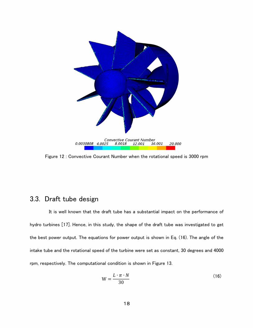
Figure 12 : Convective Courant Number when the rotational speed is 3000 rpm ............ １８

Figure 13 : Computational condition for the rim-drive .................................................................. １９

Figure 14 : Power output with for different draft tube angles .................................................... １９

Figure 15 : Velocity profiles with 12 deg. tube (top) and 36 deg. tube (bottom) ................ ２０

Figure 16 : Cross sectional view of the guide vanes in the elbow. Case (a): Without guide

vane. Case (b): Two flat guide vanes. Case (c): One flat guide vane. Case (d): One

curved guide vane. ................................................................................................................................ ２１

Figure 17 : Pressure distribution (a) without guide vanes (b) with two flat guide vanes .. ２

２

Figure 18 : 2D sketch for the elbow with one flat guide vane .................................................... ２３

Figure 19: Mass flow rate (left) and pressure drop (right), flat guide vane ........................... ２３

Figure 20: 2D sketch for the elbow with a curved guide vane ................................................... ２４

Figure 21: Mass flow rate (left) and pressure drop (right), curved guide vane ................... ２５

Figure 22 : Standard derivation of pressure drop; one flat guide vane(left), curved guide

vane (right) ............................................................................................................................................... ２６

Figure 23 : Configuration of the system ............................................................................................... ２７

Figure 24: Mass flow rate of the CFD and experiment .................................................................. ２８

Figure 25 : Power output of the CFD and experiment ................................................................... ２８

Figure 26: Comparison CFD corrected for presence of air with the experiment .............. ３０

Figure 27 : The part causing friction ...................................................................................................... ３１

Figure 28 : Comparison CFD corrected for presence of air and friction with the

experiment................................................................................................................................................ ３２

Figure 29 : Corrected power output Wf and experimental results with the error bar .... ３６

Figure 30: Tip vortex cavitation on a propeller [b] .......................................................................... ３９

Figure 31: Cavitation cloud on the suction surface of a hydrofoil [3] .................................... ３９

Figure 32: Sheet cavitation on the suction surface of a hydrofoil [34] ................................. ４０

vi

Figure 33 : Convective Courant Number on the stator when it runs at 3000rpm without

any air injection...................................................................................................................................... ４１

Figure 34 : Computational domain and the mesh around the system ..................................... ４２

Figure 35 : VVF in different mesh conditions; 1.9M, 3.6M, 5.2M ................................................ ４２

Figure 36 : Wall Y+ on the turbine when it runs at 1000rpm ....................................................... ４３

Figure 37: Configuration of the air injection hole of Design A ................................................... ４４

Figure 38: Configuration of the air injection hole of Design B ................................................... ４５

Figure 39: Contour plots of VVF without air injection when the rotational speed is

1000rpm – 4000rpm, real time is 0.3 (s) ..................................................................................... ４６

Figure 40 : Time history for the surface averaged VVF over the suction side of the blade

......................................................................................................................................................................... 47

Figure 41: Profile of pressure on the air injection hole ................................................................... 50

Figure 42 : Contour plots of time averaged absolute pressure over the turbine ................. 50

Figure 43 : Profile of mass flow rate of air from the air injection hole when the applied

pressure on the holes is 51.7kPa and the turbine runs at 2000rpm ................................ 51


pressure on the holes is 51.7kPa and the turbine runs at 2000rpm ................................ 51

Figure 45: Traveling air injected into the system ............................................................................... 52

Figure 46: 17 cross sections over the runner and draft tube ....................................................... 54

Figure 47 : profile of surface and time averaged VVF when the rotational speed is

3000rpm ....................................................................................................................................................... 55

Figure 48 : Profile of surface and time averaged absolute pressure at each cross

section when the rotational speed is 3000rpm, No-air case .............................................. 55

Figure 49 : Profile of surface and time averaged AVF when the rotational speed is

3000rpm ....................................................................................................................................................... 56

Figure 50: Contour plots of fc at cross section of the turbine (the rotational speed is

3000rpm and pressure on the air injection holes is 137.9kPa) .......................................... 56

Figure 51 : Comparison of 68.9kPa and 137.9kPa air injection in terms of depth of air

penetration and reduction of cavitation when the rotational speed is 1000rpm........ 60


penetration and reduction of cavitation when the rotational speed is 3000rpm........ 61

Figure 53: Profile of surface and time averaged VVF over the suction side of blade ....... 62

Figure 54: Profile of surface and time averaged VVF over the hub ......................................... 62

Figure 55: Contour plots of time averaged AVF over the turbine and cross sections a, b,

c and d when the rotational speed is 1000rpm and pressure on the air holes is

137.9kPa. ..................................................................................................................................................... 63

Figure 56: Contour plots of time averaged AVF and VVF over the turbine when the

rotational speed is 1000rpm; air injected by 103.4kPa from the Design B(top), air

injected 137.9kPa from the Design A (bottom) ......................................................................... 67

Figure 57 : Profile of surface and time averaged VVF over the hub, Design B ................. 68

vii

Figure 58 : Profile of surface and time averaged VVF over the suction side of blade,

Design B ...................................................................................................................................................... 68

Figure 59: Efficiency drop of the turbine when air is injected from the Design B ............. 69

Figure 60: Profile of VVF over the blade .............................................................................................. 70

Figure 61 : Configuration of the computational domain and the inlet Boundary Condition

......................................................................................................................................................................... 72

Figure 62 : Power output with different inlet condition ................................................................... 74

Figure 63 : Surface and time averaged pressure at the inlet ...................................................... 75

Figure 64 : Surface and time averaged VVF over the suction side of the blade with

constant mass flow rate inlet condition ....................................................................................... 76

Figure 65 : Surface and time averaged VVF over the blade with constant mass flow

rate inlet condition ................................................................................................................................. 76

Figure 66 : Surface and time averaged WVF over the blade with constant mass flow

rate inlet condition at the each cross section; 1000rpm and 137.9kPa air injection 77

viii

LIST OF TABLES

Table 1 : Mesh conditions for cases (a), (b) and (c) ........................................................................ １４

Table 2: Range and accuracy of tools used for the experiment ................................................ ３２

Table 3: Data from the experiment, uncertainty and fractional uncertainty of torque ... ３３

Table 4: Data from the experiment, uncertainty and fractional uncertainty of rotational

speed .......................................................................................................................................................... ３４

Table 5: Data from the experiment, uncertainty and fractional uncertainty of rotational

mass flow rate ........................................................................................................................................ ３４

Table 6: Data from the experiment, fractional uncertainty, and uncertainty of power

output ......................................................................................................................................................... ３５

Table 7 : Cavitation number in different rotational speed ............................................................ ４６

Table 8:VVF, power, and mass flow rate for No air injected case .............................................. 48

Table 9: VVF, power, and mass flow rate; Design A, 51.7(kPa) on air injection holes ....... 49

Table 10: Air injection Design A compared to No-air case when the rotational speed is

1000rpm ....................................................................................................................................................... 58


2000rpm ....................................................................................................................................................... 59


3000rpm ....................................................................................................................................................... 59


4000rpm ....................................................................................................................................................... 59

Table 14: Air injection Design B compared to No-air case when the rotational speed is

1000rpm ....................................................................................................................................................... 65

Table 15 : Air injection Design B compared to No-air case when the rotational speed is

2000rpm ....................................................................................................................................................... 65


3000rpm ....................................................................................................................................................... 66

Table 17: Air injection Design B compared to No-air case when the rotational speed is

4000rpm ....................................................................................................................................................... 66

Table 18: VVF over the blade and hub, Mass flow rate and Power when the turbine

rotates at 300rpm ................................................................................................................................... 70


1000rpm and the inlet mass flow rate is 35.23kg/s ................................................................ 73







Table 23: Efficiency drop (%) of the turbine in different rotational speed cases ................. 75

ix

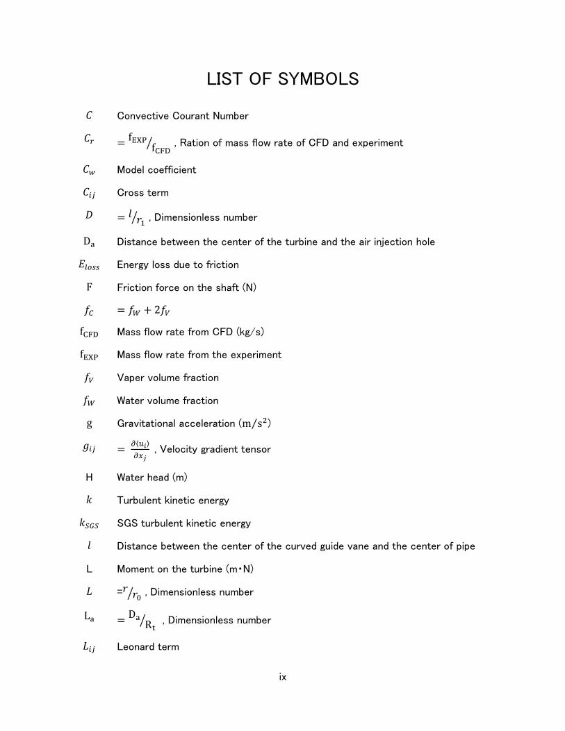
LIST OF SYMBOLS

𝐶 Convective Courant Number

𝐶𝑟 =fEXP

fCFD⁄ , Ration of mass flow rate of CFD and experiment

𝐶𝑤 Model coefficient

𝐶𝑖𝑗 Cross term

𝐷 = 𝑙 𝑟1⁄ , Dimensionless number

Da Distance between the center of the turbine and the air injection hole

𝐸𝑙𝑜𝑠𝑠 Energy loss due to friction

F Friction force on the shaft (N)

𝑓𝐶 = 𝑓𝑊 + 2𝑓𝑉

fCFD Mass flow rate from CFD (kg/s)

fEXP Mass flow rate from the experiment

𝑓𝑉 Vaper volume fraction

𝑓𝑊 Water volume fraction

g Gravitational acceleration (m s2⁄ )

𝑔𝑖𝑗 = 𝜕⟨𝑢𝑖⟩

𝜕𝑥𝑗 , Velocity gradient tensor

H Water head (m)

𝑘 Turbulent kinetic energy

𝑘𝑆𝐺𝑆 SGS turbulent kinetic energy

𝑙 Distance between the center of the curved guide vane and the center of pipe

L Moment on the turbine (m・N)

𝐿 =𝑟 𝑟0⁄ , Dimensionless number

La =Da

Rt⁄ , Dimensionless number

𝐿𝑖𝑗 Leonard term

x

N Rotational Speed (rpm)

p pressure

P = 𝑝 𝜌⁄

PV Vapor pressure

P∞ Reference pressure

Q Mass flow rate of water (kg/s)

𝑟 Distance between the guide vane and the center of the pipe (m)

𝑟0 Radius of the pipe (3 inches)

𝑟1 Radius of the curved guide vane

𝑅 =𝑟0𝑟1⁄ , Dimensionless number

Rt Radius of the turbine

𝑅𝑖𝑗 Reynolds stress term

𝑅𝑠ℎ𝑎𝑓𝑡 Radius of the shaft

𝑆𝑖𝑗 Strain rate tensor

𝑆α𝑖 source or sink of the 𝑖th phase.

u Velocity

𝑢𝜏 Friction velocity

U∞ Reference velocity

U(∅) Uncertainty of ∅

𝑥𝑖 Physical coordinate system

W Power output (W)

Wb Power output corrected for air bubble

WCFD Power output from CFD

𝑦 Wall distance

𝑌+ =𝑢𝜏𝑦

𝜈 , normalized wall distance

xi

𝑧 The distance from the water head to the center of the turbine

∀𝑐 Control volume

∀𝑖 Volume of the 𝑖th phase in a control volume

⟨ ⟩ Filtering operator

~ SGS components

xii

LIST OF GREEK LETTERS

α Fraction function

α𝑖 𝑖th phase volume fraction

𝛿𝑖𝑗 Kronecker delta

Δ Filter width

∆t Time step size

𝜃 Angle (degree)

η Efficiency of the turbine

𝜂𝐴𝑖𝑟 Efficiency of the turbine when air is injected

𝜂𝑁𝑜−𝑎𝑖𝑟 Efficiency of the turbine of No-air injected case

𝜈, 𝜈𝑡 , 𝜈𝑆𝐺𝑆 Kinematic viscosity, eddy viscosity, SGS eddy viscosity

𝜌 Density

ρ𝑖 Density of the 𝑖th phase

ρL Liquid density

𝜙 any equivalent property

𝜎 Cavitation number

xiii

LIST OF ABBREVIATIONS

AVF Air volume fraction

CFD Computational Fluid Dynamics

GS Grid Scale

LES Large Eddy Simulation

Re Reynolds number

rpm Revolutions per minute

SGS Sub Grid Scale

VOF Volume Of Fluid

VVF Vapor Volume Fraction

xiv

ACKNOWLEDGMENTS

I would first like to thank my thesis advisor Prof. Ryoichi Amano. Without his kind help,

I would not be able to study here, at the University of Wisconsin-Milwaukee. The door to Prof.

Amano’s office was always open whenever I had questions about my research, and he was so

generous and patient particularly in the beginning of my research.

This work would not have been possible without the financial support from DOE and

UWM fund. I am grateful to all of those with whom I have had the pleasure to work during this

project. I would especially like to thank Tarek Elgammal. As my friend and coworker of this

project, he has taught me more than I could give him credit for here. He has shown me, by his

example, what a good scientist and person should be.

I also like to show my appreciation to Prof. Suga from Osaka Prefecture University. He

has been supportive of my career goals and always give me personal and professional guidance

and taught me a great deal about both scientific research and life in general.

I would also like to thank the members of the committee, Prof. Istvan Lauko, and

Prof. John Reisel, for their valuable comments and fair thesis assessment.

I also want to say thank to my friends I met here. They made my stay here in America

precious. Thank you Ming, Sravan, Sai, Yash, Sophia, Teresa, John, Cynthia, Johnny, Alex, Neah,

Luke, Prayag, Paulo, Vera, Violeta, Sam, Ines, Mandana, Ahmad, Muhannad, Hanseul, Seougbum,

xv

Sanghee, Hiroto, Keita, Yuya, Hinako, Satoshi, Arisa and so many more I cannot possibly list

them all.

Nobody has been more important to me in the pursuit of this project than the members

of my family. I would like to thank my parents, whose love and guidance are with me in whatever

I pursue. I would like to give the greatest of thanks to my family for the all they have done for

me.

１

1. Introduction

Hydro-electric power, using the energy of rivers has become one of the highly reliable

renewable energy sources especially in countries with many water sources. Hydropower

supplies 16% of worldwide electricity production presently [1]. In addition to that, 86% of the

renewable energy is generated from hydropower [2]. Since most large rivers have already been

equipped with power stations, more and more attention is turning to small hydropower. Even

though the power from each station is low, they can generate a tremendous amount of power

aggregately. For this reason, making an efficient hydroelectric power system for small river

or low heads is necessary.

Hydro-turbines are set to take advantage of head differences between water levels

and to derive the power from the energy of falling water. In this study, since the aim is to make

an efficient hydroelectric power system for low heads, a Kaplan turbine, which is capable of

working efficiently with low heads and high flow rates has been selected as the turbine of the

system.

Easy assembly and durability of the scheme have to be considered in terms of minimum

maintenance of hydroelectric power system. To make installation easy and straightforward, the

integrated design developed under the DOE STTR/SBIR grant [3], which includes a rim in the

２

outside of the turbine runner to house the electrical generator rotor, was used in this study.

Regarding durability, air injection treatment for cavitation was also investigated in this study.

Cavitation is a transforming phenomenon from liquid to vapor when it is subjected to

reduced pressures at constant ambient temperature. Cavitation is the process of boiling a

liquid as a result of pressure reduction rather than heat addition. Figure 1 visually shows the

difference between boiling and cavitation. When cavitation bubble collapse in liquid, the vapor

is compressed rapidly by liquid phase, which has larger inertia and causes very high

temperature and high pressure locally and instantaneously. In addition to that, cavitation

bubbles can easily change their shape to non-spherical with affected ambient force and flow

fields. In the process of transforming the shape of bubbles, it induces a liquid jet, whose velocity

can be the order of the sound velocity of the liquid. When the liquid jet penetrates the bubble

interface, and the bubbles become toroidal, it causes a high-pressure shock wave. These liquid

jets and destructive shock wave due to the collapse of cavitation bubbles are the cause of

performance degradation of fluid machinery and material damages. Figure 2 shows a picture of

cavitation damage on turbine blades. Various studies on cavitation have been conducted for a

long time to prevent deteriorating performance and erosion due to cavitation [4].

Cavitation is problematic not only because it causes erosion but also because it is a

restriction for designing fluid machinery such as pumps and turbines to prevent erosion

happening [4]. As a method to mitigate cavitation around hydro turbines, Arndt et al. proposed

３

air injection treatment [5]. Zhi-yong et. al. investigated experimentally and theoretically the

cavitation control by aeration. The experimental results show that aeration remarkably

increases the pressure in cavitation region [6]. Revetti et al. did research on the means of air

injection to mitigate tip vortex cavitation of a Kaplan turbine and found that air injection can

decrease the level of vibration of the system and damages due to tip vortex cavitation [7].

However, the effect of air injection when hydro turbines are cavitating with cloud or sheet

cavitation have not studied enough. Hence, in this study, the effect of air injection when hydro

turbines have strong cavitation such as cloud and sheet cavitation are investigated by CFD.

Figure 1: Sketch of the water phase diagram [8]

４

Figure 2: Cavitation damage on the blades at the discharge from a Francis turbine [9]

５

2. Approach

2.1. CFD

Turbulent flow is such familiar phenomena which one can see in one’s daily life that

many industrial products are designed by considering the effects of turbulent flow. For example,

to make an aircraft of which wings can enhance the fuel efficiency and to produce a car with

reduced aerodynamic drag, it is necessary to consider the effects of turbulent flow. Since the

turbulent flow is a complicated phenomenon, it is often difficult to predict the fluid flow

experimentally, especially when the geometry where the fluid is flowing complexly. Hence, it is

required to run simulations to predict the turbulent fluid flow and to get the optimized design

of industrial products, utilizing a Computational Fluid Dynamics (CFD) [10]. In this study, CFD

was conducted by using the commercial codes of the multidisciplinary STAR CCM+. The

Volume of Fluid (VOF) and Large Eddy Simulation (LES) models were chosen to solve the

unsteady multi phase turbulent flow. As an eddy viscosity model, the WALE (Wall-Adapting

Local-Eddy Viscosity) subgrid scale model was chosen in this study.

2.2. Large Eddy Simulation

There are various eddies in the range of large scales to small scales in a turbulence

field. To simulate the significantly small eddies directly, it is necessary to use an extremely

fine mesh which can resolve the small-scale eddies. However, resolving all kinds of scales of

eddies is unrealistic in industry due to the high computational cost because it is required to

６

use at least more than 𝑅𝑒94⁄ grids to capture the smallest eddies, namely Kolmogorov scale.

Moreover, a time step must be smaller as the mesh size becomes smaller in order to make the

simulation stable and meet the Courant-Friedrichs-Lewy requirement, which results in the

extremely high computational cost. Hence, using the fine mesh which can resolve all kinds of

eddies is not suitable for industrial applications.

To solve this problem, LES decomposes the turbulent flow into Grid Scale (GS) eddies

which are larger than the grid size and Sub-Grid Scale (SGS) eddies which are smaller than

the grid size. Modeling the SGS eddies, which are independent of the geometry, and calculating

the GS eddies directly can make it possible to simulate turbulence precisely with a relatively

coarse mesh. This method is called the Large Eddy Simulation (LES).

Figure 3: The decomposition into the GS eddies and SGS eddies

７

2.3. Governing Equations of LES [11] The LES needs to classify eddies into GS eddies and SGS eddies as shown in Figure 3.

This operation is called a filtering operation. The velocity u is separated in this way by

employing the filtering operator ⟨ ⟩.

The governing equations for LES can be derived by applying box filtering operation to the

continuity equation and Navier-Stokes equations.

These equations include filtering averaged value ⟨ ⟩ and the unknown third term on the right-

hand side of Eq. (3), which is the first derivative of SGS stress 𝜏𝑖𝑗 = ⟨𝑢𝑖𝑢𝑗⟩ − ⟨𝑢𝑖⟩⟨𝑢𝑗⟩. Hence,

this equation is not closed. The physical model for SGS stress, namely SGS model, is needed

to be introduced in order to close these governing equations. SGS stress is separated in the

following way.

where,

• 𝐿𝑖𝑗：Leonard term

This term expresses a part of stress given to GS eddies because of the interaction with SGS

eddies. The Lenard term controls a part of energy dissipation of GS eddies.

𝑢(𝑥) = ⟨𝑢(𝑥)⟩⏟ 𝐺𝑆 𝑣𝑒𝑙𝑜𝑐𝑖𝑡𝑦

+ 𝑢(𝑥)̃⏟ 𝑆𝐺𝑆 𝑣𝑒𝑙𝑜𝑐𝑖𝑡𝑦

(1)

𝜕⟨𝑢𝑖⟩

𝜕𝑥𝑖= 0 (2)

𝜕⟨𝑢𝑖⟩

𝜕𝑡+ ⟨𝑢𝑗⟩

𝜕⟨𝑢𝑖⟩

𝜕𝑥𝑗= −

1

𝜌

𝜕⟨𝑝⟩

𝜕𝑥𝑖+𝜕

𝜕𝑥𝑗(𝜈𝜕⟨𝑢𝑖⟩

𝜕𝑥𝑗) −

𝜕𝜏𝑖𝑗

𝜕𝑥𝑗

(3)

𝜏𝑖𝑗 = ⟨𝑢𝑖𝑢𝑗⟩ − ⟨𝑢𝑖⟩⟨𝑢𝑗⟩

= ⟨(⟨𝑢𝑖⟩ + 𝑢�̃�)(⟨𝑢𝑗⟩ + 𝑢�̃�)⟩ − ⟨𝑢𝑖⟩⟨𝑢𝑗⟩

= ⟨⟨𝑢𝑖⟩⟨𝑢𝑗⟩⟩ − ⟨𝑢𝑖⟩⟨𝑢𝑗⟩⏟ 𝐿𝑖𝑗

+ ⟨⟨𝑢𝑖⟩𝑢�̃� + ⟨𝑢𝑗⟩𝑢�̃�⟩⏟ 𝐶𝑖𝑗

+ ⟨𝑢�̃�𝑢�̃�⟩ ⏟ 𝑅𝑖𝑗

(4)

８

• 𝐶𝑖𝑗：Cross term

𝐶𝑖𝑗 also controls a large part of energy dissipation of GS eddies with 𝐿𝑖𝑗 . In the case where

box filter is applied, ⟨𝑢𝑖𝑢𝑗⟩ − ⟨𝑢𝑖⟩⟨𝑢𝑗⟩ is directly modeled because 𝐶𝑖𝑗 becomes zero. 𝐶𝑖𝑗 and

𝐿𝑖𝑗 both have almost the same values and the effect of these two terms are normally neglected

because they cancel out each other.

• 𝑅𝑖𝑗：Reynolds stress term

SGS modeling refers to the modeling for SGS Reynolds stress term 𝑅𝑖𝑗 . This term controls a

large part of the effect on GS eddies by SGS eddies and have to include the effect of the

energy dissipation. The eddy viscosity model, which defines the stress caused by turbulence

eddies from the analogy of molecular viscous stress, is widely used for RANS and Reynolds

stress is defined as the following:

The model which applies the same idea as that of eddy viscosity model for RANS is called SGS

eddy viscosity model. Since the parameter which has to be modeled is SGS Reynolds stress,

this is modeled by SGS turbulence kinetic energy 𝑘𝑆𝐺𝑆 and SGS eddy kinematic viscosity 𝜈𝑆𝐺𝑆

as shown in Eq. (6).

𝑢𝑖′𝑢𝑗′̅̅ ̅̅ ̅̅ =2

3𝛿𝑖𝑗𝑘 − 2𝜈𝑡 (

𝜕𝑢�̅�𝜕𝑥𝑗

+𝜕𝑢�̅�

𝜕𝑥𝑖)

(5)

𝜏𝑖𝑗 = ⟨𝑢�̃�𝑢�̃�⟩ =2

3𝛿𝑖𝑗𝑘𝑆𝐺𝑆 − 2𝜈𝑆𝐺𝑆 (

𝜕⟨𝑢𝑖⟩

𝜕𝑥𝑗+𝜕⟨𝑢𝑗⟩

𝜕𝑥𝑖)

(6)

９

2.4. WALE subgrid scale model [12] The WALE (Wall-Adapting Local-Eddy Viscosity), Subgrid Scale model, is an eddy

viscosity model, of which length scale is filtered width Δ. In WALE model, the SGS eddy

viscosity ν𝑆𝐺𝑆 is defined as following by using the filter width Δ:

, where the strain rate tensor 𝑆𝑖𝑗, 𝑔𝑖𝑗 and the tensor 𝑆𝑖𝑗𝑑 are respectively defined as following;

In this study, the model coefficient 𝐶𝑤 is set as 𝐶𝑤 = 0.544.

2.5. Volume of Fluid (VOF)

The Volume of Fluid (VOF) method has been given by Noh and Woodward in 1976

[13], where fraction function α (see Eq.(11)) appeared, although the first publication by Hirt

and Nichols in 1981 [14]. The VOF model assumes that all immiscible fluid phases present in

a control volume share velocity, pressure, and temperature fields. Therefore, the same set of

basic governing equations describing momentum, mass, and energy transport in a single-phase

flow is solved. The properties solved by this method are defined as following by using the (i)th

phase volume fraction (α𝑖)

𝜈𝑆𝐺𝑆 = 𝐶𝑤Δ2

(𝑆𝑖𝑗𝑑𝑆𝑖𝑗

𝑑)3 2⁄

(𝑆𝑖𝑗𝑑𝑆𝑖𝑗

𝑑)5 4⁄

+ (𝑆𝑖𝑗𝑆𝑖𝑗)5 2⁄

(7)

𝑆𝑖𝑗 =1

2(𝜕⟨𝑢𝑖⟩

𝜕𝑥𝑗+𝜕⟨𝑢𝑗⟩

𝜕𝑥𝑖)

(8)

𝑔𝑖𝑗 = 𝜕⟨𝑢𝑖⟩

𝜕𝑥𝑗 (9)

𝑆𝑖𝑗𝑑 =

1

2(𝑔𝑖𝑗

2 + 𝑔𝑗𝑖2 ) −

𝛿𝑖𝑗

3𝑔𝑘𝑘2 , 𝑔𝑖𝑗

2 = 𝑔𝑖𝑘 𝑔𝑘𝑗 (10)

α𝑖 =∀𝑖∀𝑐 (11)

https://en.wikipedia.org/wiki/Volume_of_fluid_method#cite_note-Noh76-1

https://en.wikipedia.org/wiki/Volume_of_fluid_method#cite_note-2

１０

where 𝜙 is any equivalent property. The conservation equation that describes the transport of

volume fractions is:

where 𝑆α𝑖 is the source or sink of the i th phase. The equation considers the phase motion

relative to the reference frame motion (u − urf).

The fluid interface is found by rapic change of the value of volume fraction α. When a

cell is empty with no traced fluid inside, the value of α is zero. When the cell is full, α = 1.0.

When there is a fluid interface in the cell, 0 < α < 1.0. α is a discontinuous function. In other

words, its value jumps from 0 to 1 when the argument moves into the interior of traced phase.

Hence, the fluid interface is found where the value of α changes most rapidly.

2.6. Experiment setup

The hydro turbine loop is designed to run a horizontally oriented 0.0762m Kaplan

turbine from a relatively low water height (3m maximum level) between the head and sink. The

system is a closed system. Water flows from the head tank to the turbine, discharging to the

sink tank, and then the system pumps the water again from the sink tank to the head one. The

3D CAD of the system is shown in Figure 4.

𝜙 =∑α𝑙 𝜙𝑙

𝑛

𝑙=1

(12)

∂

∂t∫α𝑖 d∀.

∀

+∫α𝑖 (u − urf) dA.

A

= ∫(𝑆α𝑖 −α𝑖ρ𝑖 Dρ𝑖Dt) d∀

.

∀

(13)

１１

The experiment system is composed of a tank, a pump to circulate the water, two flow

meters (one before the tank and one in the overflow pipe), and a turbine. Although Rim-drive

generator usually does not have any shaft, the runner in this experiment system has a shaft

for measuring the speed and torque. As seen in Figure 5, this shaft was connected to a Magtrol

torque-meter and a DC generator. Electric power dissipates in a resistive load bank. The flow

rate was measured by a Badger-Meter electromagnetic flow-meter, Model M-2000 M-Series

Mag meter. The rotational speed of the runner was measured by Omega HHT13 Tachometer.

Figure 4 : 3D CAD of the experimental system

Figure 5 : The experiment system

１２

2.7. Turbine design

The 3-inch diameter turbine design was developed by Turbine Builder design software

[15] and then 3D CAD was built and exported to the CFD model. The rotor blade has an aspect

ratio of 1.0, the thickness-chord ratio of 0.07, and count of 5 blades. The geometrical layout

of the turbine is shown in Figure 6. The turbine and stator for the experiment were 3D printed.

As shown in Figure 7, the runner has a slot to slide the electrical generator. The material

selected for the runner and stator manufacturing was Eastman Amphora 3D Polymer AM3300

marketed by ColorFabb as nGen [16].

Figure 6 : Geometrical layout of the turbine

１３

Figure 7 : Turbine and stator made by 3D printer

１４

3. CFD development for Rim-Drive

3.1. Mesh size

Three kinds of polyhedral meshes were initially tested around the turbine to examine

the effect of the mesh size. The detail of these meshes is shown in Table 1. Figure 8 shows

the mesh resolution around the runner in each case. The power output was chosen as the

parameter to check the mesh independence. As shown in Figure 9, The difference of power

output is 6.4% between 0.8 million and 1.5 million setups and 10.4% between 1.5 million and 4.4

million setups. Considering the time management and the accuracy of the CFD, a mesh

with 1.5million cells was selected for this study.

It is important to have fine enough mesh near the wall to get precise simulation results

because the amount of change of physical value such as velocity is significantly big there. To

check if the mesh near the wall is fine enough, dimensionless distance 𝑌+, defined by Eq.(14),

is checked. Figure 10 shows the mesh around the rotor and stator. Although the maximum of

𝑌+ was 25, 𝑌+was kept less than 2.5 almost all over the stator and turbine.

Table 1 : Mesh conditions for cases (a), (b) and (c)

𝑌+ =𝑢𝜏𝑦𝜈 (14)

Number of Cells 0.8 Million 1.5 Million 4.4 Million

Computational Time 1.0x 1.9x 5.5x

Simulation Detail Coarse Fine Very Fine

１５

Figure 8 : Mesh resolution ; (a) coarse 0.8 M (b) fine 1.5M (c) very fine 4.4M

Figure 9: Power output versus mesh size

１６

3.2. Time step

A time step ∆t = 10−4(s) was chosen for the simulation of the entire system. In order

to verify the condition of the mesh, and the time step, the Convective Courant Number C

around the runner and stator were checked. The Convective Courant Number C is the

dimensionless transport per time step and defined as Eq.(15) in the one-dimensional case. This

number is widely used to check if the size of the time step is proper or not. For example, if the

courant number is 1, the flow of a certain point advances to the next element at the next

moment as shown in the upper diagram of Figure 11. Therefore, the original analysis accuracy

Figure 10 : 𝑌+ around the stator and runner when the rotational speed is 3000 rpm

１７

of the mesh can be obtained. On the other hand, if the Courant number is 10, the flow goes

forward by the 10 elements at the next moment as shown in the lower diagram of Figure 11,

passing through the nine elements during that time. Therefore, the accuracy will be as same

as simulations with 10 times coarse mesh. As Figure 12 shows, the Convective Courant Number

is less than 2.0 over almost all area on the stator and runner.

𝐶 =𝑢Δ𝑡

Δ𝐿 (15)

Figure 11 : The image of flow with different Courant number

１８

3.3. Draft tube design

It is well known that the draft tube has a substantial impact on the performance of

hydro turbines [17]. Hence, in this study, the shape of the draft tube was investigated to get

the best power output. The equations for power output is shown in Eq. (16). The angle of the

intake tube and the rotational speed of the turbine were set as constant, 30 degrees and 4000

rpm, respectively. The computational condition is shown in Figure 13.

Figure 12 : Convective Courant Number when the rotational speed is 3000 rpm

W =𝐿 ∙ 𝜋 ∙ 𝑁

30 (16)

１９

Five kinds of draft tube angles were tested in this study. Figure 14 shows the profile

of the power output with different draft tube angle. For the greater value of the draft tube

angle, it is seen that the flowing water leave the boundary and cause separations, which bring

down the efficiency of draft tubes (see Figure 15). Hence, there is a tendency that less draft

tube angle gives more power output (see Figure 14). Considering the limitation of the lab space

of the room, a 15-degree draft tube angle was selected at the end.

Figure 13 : Computational condition for the rim-drive

Figure 14 : Power output with for different draft tube angles

２０

3.4. Investigation of guide vanes at the 90-degree elbow

The experimental system includes a 90-degree elbow just upstream of the turbine

(see Figure 4). Such an elbow causes flow skewness and eddies due to the sudden change in

flow direction when the flow enters the elbow. Of course, the best policy is to avoid or minimize

such discontinuities, but this is not always practical. One of the ways to minimize the problem

caused by the sudden change of the flow direction is the use of guide vanes. Hence, in this

study, four kinds of guide vanes in the elbow, shown in Figure 16, were examined.

Figure 15 : Velocity profiles with 12 deg. tube (top) and 36 deg. tube (bottom)

２１

Figure 17 illustrates the ability of the guide vanes to straighten the flow in the elbow.

As the disadvantage of the guide vane, it was found that the guide vanes caused an energy

loss due to the friction between the flow and the guide vanes.

Figure 16 : Cross sectional view of the guide vanes in the elbow. Case (a): Without guide

vane. Case (b): Two flat guide vanes. Case (c): One flat guide vane. Case (d): One curved

guide vane.

２２

Firstly, Optimization study for the Case(c) was conducted. To consider the effect of

the position of the guide vane, a new dimensionless parameter (L) was defined for the flat guide

vanes to express the guide vane position concerning the center of the elbow:

where 𝑟 is the distance between the guide vane and the center of the pipe, and 𝑟0 is the radius

of the pipe, which is constant at 0.0762m in this case. Also, the angle θ is defined as the ending

point of the guide vane as shown in Figure 18.

Figure 17 : Pressure distribution (a) without guide vanes (b) with two flat guide vanes

𝐿 = 𝑟 𝑟0⁄ (17)

２３

Three values of θ (30, 60 and 90 degrees) and three values of L (0.33, 0.50 and 0.67)

were used for the flat guide vane, and the mass flow rate and the pressure drop were checked

(Figure 19). From this result, the position of the guide vane (L) does not affect the mass flow

rate and pressure drop. Besides, there is a tendency of more mass flow rate and less pressure

drop with larger θ. Hence, 90-degree is the best among of 30, 60 and 90-degree guide vanes.

Figure 18 : 2D sketch for the elbow with one flat guide vane

Figure 19: Mass flow rate (left) and pressure drop (right), flat guide vane

２４

Secondary, an optimization study for the Case(d) was conducted. Two other

dimensionless parameters (𝑅 and 𝐷) were defined for the curved guide vane case. The details

are shown in Figure 20 and Eq. (18) and Eq. (19). In the case of the one flat guide vane, it was

discovered 90-degree guide vane was the best in terms of maximizing mass flow rate and

minimizing pressure drop. Hence, in the study of Case(d), θ was set as constant as 90 degrees.

The profile of mass flow rate and pressure drop are shown in Figure 21. There is a tendency

that larger D and smaller R gives more mass flow rate and less pressure drop because of less

wet area of the guide vane which cause friction loss.

Figure 20: 2D sketch for the elbow with a curved guide vane

𝑅 =𝑟0𝑟1⁄ (18)

𝐷 = 𝑙 𝑟0⁄ (19)

２５

According to these different guide vane cases, regarding energy, the best choice is not

to install any guide vane. However, another factor needs to be considered, particularly for a

hydro turbine which is to operate on a continuous basis with minimum maintenance. The

pressure fluctuations observed in the pipe could induce vibrations and cause turbine wear.

While the standard derivation of pressure drop in the case of without any guide vane was 7.9

Pa, as Figure 22 shows, any guide vane at the elbow can reduce the pressure fluctuation in

the pipe. If this is a concern, some guide vanes can be implemented in the system, benefiting

maintenance needs at the cost of a small energy loss due to the friction on guide vane surfaces.

Figure 21: Mass flow rate (left) and pressure drop (right), curved guide vane

２６

Figure 22 : Standard derivation of pressure drop; one flat guide vane(left), curved guide

vane (right)

２７

4. Result and discussion on Rim-Drive

4.1. Initial data

Considering the study of draft tubes and guide vanes, a 15-degree draft tube and

elbow without any guide vane were selected for the experiment and CFD setup. The

configuration of the system is shown in Figure 23. The CFD and experiment were conducted

with 2.0m water head and the result is shown in Figure 24 and Figure 25. As Figure 24 and

Figure 25 show, there is significant disagreement between CFD and experiment. In the next

section, the causes of these disagreements are discussed.

Figure 23 : Configuration of the system

２８

Figure 24: Mass flow rate of the CFD and experiment

Figure 25 : Power output of the CFD and experiment

２９

4.2. Presence of air

Figure 24 shows that the mass flow rate was less in the experiment than CFD. The

flow observed during the experiment contained air, and it is the reason why the mass flow rate

in the experimental test is less than CFD. Both the experimental and calculated flow rates are

linear with rotational speed and can be approximated from the curves by linear approximation

as following;

where N is the rotational speed, and fCFD and fEXP are the calculated and experimental flow

rates, respectively. Defining the coefficient Cr as the ratio of mass flow rate with ideal condition

(CFD) and mass flow rate from the experiment:

and assuming that the power output is proportional to the mass flow rate, we can obtain a

corrected CFD power output, Wb, as taking into account the effect of air in the system. The

correction is expressed in the equation below, and the results are plotted in Figure 26:

fCFD = 0.0035N + 15.546 (20)

fEXP = 0.0027N + 14.20 (21)

𝐶𝑟 =fEXP

fCFD⁄ (22)

Wb = 𝐶𝑟×WCFD (23)

３０

4.3. Effect of friction

The part holding the shaft is so tight that the shaft could not rotate smoothly (see

Figure 27) in the experiment. The friction here is considered as the cause of the energy loss.

Assuming the friction force F is constant, the energy loss 𝐸loss(W) is defined as;

where 𝑅𝑠ℎ𝑎𝑓𝑡 (m) is the radius of the shaft (0.0079m) and N is the rotational speed per minute

(rpm). The constant force F can be determined from the experimental point where there is no

output, 3,000 rpm, when all the energy is dissipated by friction. Hence, the friction force F can

be estimated as following;

Figure 26: Comparison CFD corrected for presence of air with the experiment

𝐸𝑙𝑜𝑠𝑠 = F×(𝑅𝑜𝑡𝑎𝑡𝑖𝑜𝑛𝑎𝑙 𝑠𝑝𝑒𝑒𝑑) = 𝐹×(𝑁

602𝜋𝑅𝑠ℎ𝑎𝑓𝑡)

(24)

(𝑊𝑏)3000𝑟𝑝𝑚 = 𝐹×(3000

602𝜋×0.0079)

(25)

⇔ F = 80.6 (N) (26)

３１

By substituting Eq. (26) into Eq. (24), the energy loss 𝐸loss can be obtained. Then, the power

output 𝑊𝑓 corrected for friction can be obtained as;

The profile of 𝑊𝑓 is shown in Figure 28.

𝑊𝑓 = 𝑊𝑏 − 𝐸𝑙𝑜𝑠𝑠 (27)

Figure 27 : The part causing friction

３２

4.4. Error analysis

Table 2 sums up the measurement technique, measuring range and accuracy of

various instruments used in the experiment for various parameters. Errors in experiments can

rise from instrument conditions, calibration, environment, observation, and reading. The

accuracy of the experiment has to be validated with the aid of error analysis using the method

described by Moffat [18]

Table 2: Range and accuracy of tools used for the experiment

Quantity Measuring range Accuracy

Torque meter 0-10 (N ∙ m) ±0.01(N ∙ m) [19]

Tachometer 1-20,000 (rpm) ±0.05% [20]

Flow meter 4.7-1400 (kgs⁄ ) ±0.25% [21]

Figure 28 : Comparison CFD corrected for presence of air and friction with the experiment

３３

When the measurement value is described as ϕ ± U(ϕ), the fractional uncertainty is defined

by Eq. (28). The fractional uncertainty gives a dimensionless number that shows the relative

size of the uncertainty compared to the measurement. The torque from the experiment and

its uncertainty and fractional uncertainty is shown in Table 3. The rotational speed N (rpm)

from the experiment and its uncertainty and fractional uncertainty is shown in Table 4. The

mass flow rate from the experiment and its uncertainty and fractional uncertainty is shown in

Table 5.

Table 3: Data from the experiment, uncertainty and fractional uncertainty of torque

Experiment Number Torque (N ∙ m) Uncertainty (N ∙ m) Fractional uncertainty

1 0.000 ±0.010 2 0.066 ±0.010 ±15.09%

3 0.127 ±0.010 ±7.85%

4 0.144 ±0.010 ±6.92%

5 0.200 ±0.010 ±5.01%

6 0.278 ±0.010 ±3.60%

7 0.359 ±0.010 ±2.78%

8 0.410 ±0.010 ±2.44%

9 0.477 ±0.010 ±2.09%

(Fractional uncertainty of E) =U(ϕ)

ϕ

(28)

３４

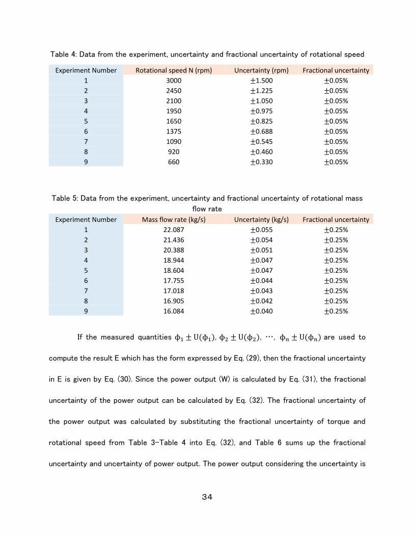
Table 4: Data from the experiment, uncertainty and fractional uncertainty of rotational speed

Experiment Number Rotational speed N (rpm) Uncertainty (rpm) Fractional uncertainty

1 3000 ±1.500 ±0.05%

2 2450 ±1.225 ±0.05%

3 2100 ±1.050 ±0.05%

4 1950 ±0.975 ±0.05%

5 1650 ±0.825 ±0.05%

6 1375 ±0.688 ±0.05%

7 1090 ±0.545 ±0.05%

8 920 ±0.460 ±0.05%

9 660 ±0.330 ±0.05%

Table 5: Data from the experiment, uncertainty and fractional uncertainty of rotational mass

flow rate

Experiment Number Mass flow rate (kg/s) Uncertainty (kg/s) Fractional uncertainty

1 22.087 ±0.055 ±0.25%

2 21.436 ±0.054 ±0.25%

3 20.388 ±0.051 ±0.25%

4 18.944 ±0.047 ±0.25%

5 18.604 ±0.047 ±0.25%

6 17.755 ±0.044 ±0.25%

7 17.018 ±0.043 ±0.25%

8 16.905 ±0.042 ±0.25%

9 16.084 ±0.040 ±0.25%

If the measured quantities ϕ1 ± U(ϕ1), ϕ2 ± U(ϕ2), …, ϕ𝑛 ± U(ϕ𝑛) are used to

compute the result E which has the form expressed by Eq. (29), then the fractional uncertainty

in E is given by Eq. (30). Since the power output (W) is calculated by Eq. (31), the fractional

uncertainty of the power output can be calculated by Eq. (32). The fractional uncertainty of

the power output was calculated by substituting the fractional uncertainty of torque and

rotational speed from Table 3-Table 4 into Eq. (32), and Table 6 sums up the fractional

uncertainty and uncertainty of power output. The power output considering the uncertainty is

３５

showed in Figure 29.

Table 6: Data from the experiment, fractional uncertainty, and uncertainty of power output

Experiment Number Power output (W) Fractional uncertainty Uncertainty (W)

1 0 2 17 ±0.151 ±2.57

3 28 ±0.079 ±2.20

4 29.5 ±0.069 ±2.04

5 34.5 ±0.050 ±1.73

6 40 ±0.036 ±1.44

7 41 ±0.028 ±1.14

8 39.5 ±0.024 ±0.96

9 33 ±0.021 ±0.69

E = C𝜙1𝑎 ∙ 𝜙2

𝑏… ∙ 𝜙𝑛𝑑

(29)

U(E)

E= ±√[𝑎

U(ϕ1)

ϕ1]2

+ [𝑏U(ϕ2)

ϕ2]2

+⋯+ [𝑑U(ϕ𝑛)

ϕ𝑛]2

(30)

W =L ∙ π ∙ N

30

(31)

W

U(W)= ±√[

U(L)

L]2

+ [U(N)

N]2

(32)

３６

4.5. Summary of experimental study

Test results from the experiment were initially far below CFD calculations. However,

the difference can be explained by the presence of air in the system and friction. The presence

of air could be reduced or eliminated with a redesign and would be expected to be less in a

larger system. Friction is due mostly to the shaft, which is not necessary for the rim-drive

system. Ultimately, with proper flow input and under the conditions set in the lab, a rim-drive

turbine should, therefore, be able to produce 250 W with very low water head: 2.04.

Figure 29 : Corrected power output Wf and experimental results with the error bar

３７

5. Cavitation treatment by air injection

5.1. Phenomenon Description

Cavitation is caused by local vaporization of the fluid when the local static pressure

of liquid falls below the vapor pressure of the liquid. Small bubbles or cavities filled with vapor

are formed, which suddenly collapse on moving forward with the flow into regions of high

pressure. These bubbles collapse with tremendous force, giving rise to as high a pressure as

1GPa [22]. In turbines, cavitation is most likely to occur at the suction side of blades. When

cavitation occurs, it causes the undesirable effects such as local pitting of the metal surface,

severe erosion [23-25], the vibration of the machine [26-28] and a drop of efficiency due to

vapor formation, which reduces the effective flow areas [29-30]. The avoidance of cavitation

in conventional designs is regarded as one of the essential tasks of turbine designers.

Cavitation imposes a limitation on the design and working condition such as speed of rotations

of the turbines [31]. In this study, the aeration treatment was investigated regarding the

reduction of cavitation and improvement of the range of rotational speed that the system can

run safely.

5.1.1. Cavitation number The cavitation number σ is used to characterize the potential of the flow to cavitate.

It is a dimensionless number defined by Eq. (33). It expresses how close the pressure in the

liquid flow is to the vapor pressure (and therefore the potential for cavitation).

３８

𝑈∞, 𝑃∞ and 𝑃𝑉 are respectively a reference velocity, reference pressure and vapor pressure

in the flow, respectively. (usually upstream quantities), and ρLis the liquid density. In this study,

the velocity and pressure entering the rotor were chosen as 𝑈∞and 𝑃∞ respectively.

5.1.2. Type of cavitation Vortex cavitation

Many high Reynolds number flows seen in industry contain a region of concentrated

vorticity where the pressure in the vortex core is often considerably smaller than in the rest

of the flow. Tip vortex cavitation is the form of cavitation inception occurs when a bubble is

trapped into the low-pressure region located in the center of the tip vortex [32]. The tip

vortices of ship's screws or pump impellers are a typical example of this (see Figure 30).

Cloud cavitation

With a further reduction in the cavitation number, it follows that the entire core of the

vortex is filled with vapor and becomes continuous due to the accumulation of individual

babbles, as illustrated by the picture in Figure 31, namely cloud cavitation.

Sheet cavitation

Another class of large-scale cavitation structures is that which occurs when a wake

or region of separated flow fills with vapor. Cavitation took place while a single vapor-filled

separation zone as illustrated in Figure 32 is called sheet cavitation.

𝜎 =P∞ − Pv12 ρLU∞

2 (33)

３９

Figure 30: Tip vortex cavitation on a propeller [b]

Figure 31: Cavitation cloud on the suction surface of a hydrofoil [3]

４０

5.2. Computational Fluid Dynamics (CFD) model setting up

5.2.1. Modeling Same as the study for the hydro turbine system with a low head, CFD approach was

performed by using the commercial codes of the multidisciplinary STAR CCM+, choosing

Volume of Fluid (VOF) and Large Eddy Simulation (LES) to solve the unsteady multi phase

turbulent flow in this study, too. The vapor pressure of water was set as 3.2 kPa, assuming the

temperature of the water is 298(K). The time step was set as 4×10−5 (s). As Figure 33 shows,

the Convective Courant Number is less than 1.0 almost all over the area of the runner, so the

time step is small enough. The rotational speed N was set in the range of 1000-4000rpm. The

stator, runner, intake and outlet tube are the same as those used in the study on rim-drive.

Figure 32: Sheet cavitation on the suction surface of a hydrofoil [34]

４１

5.2.2. Configuration and mesh

Since cavitation is a complex phenomenon which includes the formation, separation

and collapse of the cavitation bubble, it is necessary to use very fine mesh to capture the

characteristics of the flow phenomenon. Hence, to make the number of cells for the simulation

smaller, just the intake tube, stator, turbine and draft tube were selected as calculation domain

(see Figure 34). Figure 35 shows the VVF over the suction side of the turbine blade when the

rotational speed is 1000rpm, and these value of VVF were used for the mesh independent

study. The 3.6Million cells case was selected as the mesh for the latter work because of the

Figure 33 : Convective Courant Number on the stator when it runs at 3000rpm without any

air injection

４２

minimum deviation from the average (1.3 %), the better Y+representation than the 1.9 million

case, and the 67% less time consuming compared to the 5.2Million case. The Y+ was kept

less than 2.0 with using 3.6 million cells (see Figure 36)

Figure 34 : Computational domain and the mesh around the system

Figure 35 : VVF in different mesh conditions; 1.9M, 3.6M, 5.2M

４３

5.2.3. Design of air injection holes Since the turbine used in this study has a rim, it is difficult and not practical to make

air injection holes right above the turbine blade. Hence air injection holes were made at

upstream of the turbine. In this thesis, two kinds of design of air injection holes were investigated.

Firstly, air injection holes were set between blades of the stator (Design A). The diameter of

each hole is 1mm. Since the stator has nine blades, nine air injection holes were set (see Figure

37). Secondly, air injection holes were made on the blades of the stator (Design B). In this

design, each blade has three injection holes at the 0.015m, 0.025m and 0.035m from the center

Figure 36 : Wall Y+ on the turbine when it runs at 1000rpm

４４

of the stator respectively. The position of these holes can be described by the dimension less

parameter La, which is defined by Eq. (34) (see Figure 38). The diameter of these holes is

1mm.

La =DaRt (34)

Figure 37: Configuration of the air injection hole of Design A

４５

5.2.4. Boundary conditions 82.7 (kPa) was applied at the inlet as the boundary condition. As the outlet condition,

atmospheric pressure outlet was used. Non-slip boundary condition was applied on the wall.

5.3. Result and Discussion

5.3.1. No air injected case

No air injected case was first investigated to get the baseline data. The rotational

speed of the turbine was changed in the range of 1000rpm to 4000rpm. The quasi-steady state

is reached at 0.18(s), and data later than this time was used to get time averaged properties.

The cavitation number in each rotational speed case, calculated from the mean velocity and

pressure entering the turbine, are shown in Table 7. The patterns of cavitation are shown in

Figure 39 and Figure 40. As Figure 39 shows, stronger type of cavitation (sheet cavitation) was

Figure 38: Configuration of the air injection hole of Design B

４６

found for the higher rotational speed of the turbine, corresponding to the decrease of cavitation

number. The difference of cloud cavitation and sheet cavitation can be seen in Figure 40. When

the rotational speed is 1000rpm, the behavior of cavitation is randomly fluctuating due to the

vapor cloud cycle (formation, separation, and collapse). However, when the turbine is rotating

at higher speed (3000rpm or 4000rpm), the vapor volume fraction (VVF) on the suction side

of the blade is more stable, and more than 75% of the area of the suction side is covered with

vapor. As the baseline data, the VVF over the blade and hub, power output and mass flow rate

of water were obtained (see Table 8)

Table 7 : Cavitation number in different rotational speed

1000rpm 2000rpm 3000rpm 4000rpm

Cavitation number 2.71 2.05 1.55 1.17

Figure 39: Contour plots of VVF without air injection when the rotational speed is 1000rpm

– 4000rpm, real time is 0.3 (s)

４７

Figure 40 : Time history for the surface averaged VVF over the suction side of the blade

0

0.1

0.2

0.3

0.4

0.5

0.6

0.7

0.8

0.9

1

0.12 0.17 0.22 0.27

VV

F

Real time (s)

Surface averaged VVF on the blade of suctionside

1000rpm

2000rpm

3000rpm

4000rpm

48

Table 8:VVF, power, and mass flow rate for No air injected case

No Air 1000rpm 2000rpm 3000rpm 4000rpm

VVF (blade) 0.363 0.692 0.810 0.817

VVF (hub) 0.343 0.321 0.295 0.225

P(W) 612.9 1103.4 1414.2 1511.7

Mass Flow Rate (kg/s) 35.23 39.14 42.99 46.55

5.3.2. Fluctuation of pressure on the air injection hole

Firstly, 51.7(kPa) gauge pressure was applied on the air injection holes with turbine

rotating at 2000rpm in the Design A, and VVF over the blade and hub, Power output and mass

flow rate of water were obtained (Table 9). In this case, the surface and time averaged

cavitation over the suction side of the blade is 0.652, while that of baseline data is 0.692

(percentage of reduction is 5.8%). The aeration treatment could not eliminate cavitation over

the suction side of the blade well because of the fluctuation of pressure on the air injection

holes. As Figure 41 shows, the pressure on the air injection hole fluctuates when the blades

of turbine pass the hole because of the difference in pressure between the suction side and

pressure side of the blade (see Figure 42). The pressure reaches the peak right after the

passage of the blade and going down as the suction-side of the next blade get closer to the

hole. The amount of air injected into the system is determined by the difference in pressure

between the air injection hole and liquid water around the air injection hole. Since constant

pressure is applied to the air injection holes, the mass flow rate of air from the hole also

fluctuates corresponding to the fluctuation of pressure on that (see Figure 43). In order to

clear the correlation between the pressure and the mass flow rate of air, both pressure and

mass flow rate of air were normalized by their mean values, which are 122.6kPa and 0.178g/s,

49

respectively. Profile of them is shown in Figure 44, denoting the correlation of them. When the

pressure of liquid water near the hole is high (time 0.271s), the mass flow rate of air from the

hole is small. On the other hand, when the pressure is low (time 0.275), the mass flow rate of

air is significant. Figure 45 visualize how the injected air travels in the system. The air injected

during time 0.273s to 0.276s, which makes an enormous cloud of air, goes through the system

without contacting the blades of the turbine. Hence, the aeration treatment, in this case, could

not eliminate cavitation over the blades well. If it is possible to control the position of the air

injection holes to make the cloud of air injected during the pressure of water near the holes

are small contact the blades of the runner, it would be a way to utilize aeration efficiently.

However, since this study focuses on the effect of air on cavitation around the turbine, enough

amount of air (68.9kPa and 137.9kPa for the Design A and 103.4kPa and 137.9kPa for the

Design B) were injected in the following chapter.

Table 9: VVF, power, and mass flow rate; Design A, 51.7(kPa) on air injection holes

VVF (blade) VVF (hub) Power (W) Mass flow rate (kg/s)

0.652 0.317 1102.1 38.72

50

Figure 41: Profile of pressure on the air injection hole

Figure 42 : Contour plots of time averaged absolute pressure over the turbine

51


pressure on the holes is 51.7kPa and the turbine runs at 2000rpm


pressure on the holes is 51.7kPa and the turbine runs at 2000rpm

0

0.05

0.1

0.15

0.2

0.25

0.3

0.269 0.27 0.271 0.272 0.273 0.274 0.275 0.276 0.277

Mas

s fl

ow

rat

e o

f ai

r (g

/s)

Real time (s)

Profile of mass flow rate of air on the air injection hole

0

0.2

0.4

0.6

0.8

1

1.2

1.4

1.6

0.269 0.27 0.271 0.272 0.273 0.274 0.275 0.276 0.277

Real time (s)

Profile of normalized pressure and mass flow rate of air

Normalized pressure on the airinjection hole

Normalized mass flow rate of airfrom the air injection hole

52

5.3.3. Design A

In this design, two kinds of inlet pressure, 68.9kPa, and 137.9kPa gauge pressure, on

the air injection holes were tested. Air volume fraction (AVF) at the outlet, vapor volume

fraction (VVF) over the suction side of the blade and hub, mass flow rate of water, and power

output were investigated with comparison with the baseline data (No-air case).

5.3.3.1. Movement of air injected from the upstream of the turbine

In the study of aeration treatment for tip vortex cavitation, the air injection holes were

made above the turbine blade, and the air was injected directly to the area cavitation happens

[7]. However, the turbine used in this study has a rim around the turbine blades. Hence, it is

difficult and not practical to make air injection holes above the turbine blade. That is why the

air injection holes were made upstream of the turbine. Hence, it is necessary to investigate

Figure 45: Traveling air injected into the system

53

the movement of air injected from the upstream of the turbine to check if air can eliminate

cavitation.

The surface and time averaged VVF, AVF and pressure on seventeen cross sections,

shown in Figure 46, were investigated to examine the movement of air injected from upstream

of the turbine. The seventeen cross sections were set from 0.01m (x Rt⁄ =0.263) to 0.09m

(x Rt⁄ =2.37) in x direction.Figure 47 shows the VVF over these cross sections. Cavitation

starts to happen at x=0.01m (x Rt⁄ =0.263), which is the starting position of turbine blade, and

the volume of vapor increases due to cavitation happening on the turbine blades and the VVF

reaches the maximum value at x=0.025m (x Rt⁄ =0.658), which is the ending position of the

turbine blades. Then, the VVF decreases after x=0.025m (x Rt⁄ =0.658) due to the collapse of

cavitation bubbles (see Figure 47). The pressure profile over the cross sections is shown in

Figure 48. Due to the cavitation bubble, which has less pressure than liquid water, the value of

pressure reaches the minimum at x=0.025m (x Rt⁄ =0.658). Because of the pressure gradient

shown in Figure 48, the air injected into the system from upstream of the turbine stayed or

sucked at around x=0.025m (x Rt⁄ =0.658) and eliminate cavitation (see Figure 47 and Figure

49).

The movement of air at the cross section at x=0.01m ( x Rt⁄ =0.263) was also

investigated to verify that air from the upstream can eliminate cavitation. Figure 50 shows

volume fraction scenes of the three fluids (air: blue, liquid water: green, vapor: red) by

54

introducing 𝑓𝑐 , which is defined by Eq. (30). This figure shows the movement of air getting

sucked into the suction side of the blade and reducing cavitation.

𝑓𝑐 = 𝑓𝑊 + 2𝑓𝑉 (35)

Figure 46: 17 cross sections over the runner and draft tube

55

Figure 47 : profile of surface and time averaged VVF when the rotational speed is 3000rpm

Figure 48 : Profile of surface and time averaged absolute pressure at each cross section

when the rotational speed is 3000rpm, No-air case

0

0.05

0.1

0.15

0.2

0.25

0.3

0 0.02 0.04 0.06 0.08 0.1

VV

F

x(m)

Surface and time averaged VVF (3000rpm)

No-air

68.9kPa

137.9kPa

56

Figure 49 : Profile of surface and time averaged AVF when the rotational speed is

3000rpm

Figure 50: Contour plots of 𝑓𝑐 at cross section of the turbine (the rotational speed is

3000rpm and pressure on the air injection holes is 137.9kPa)

0

0.02

0.04

0.06

0.08

0.1

0.12

0.14

0.16

0.18

0.2

0 0.02 0.04 0.06 0.08 0.1

VV

F

x(m)

Surface and time averaged AVF (3000rpm)

No-air

68.9kPa

137.9kPa

57

5.3.3.2. Cavitation over the blade and hub

The results of each rotational speed are shown in Table 10- Table 13, respectively. The

percentage change (VVF increase, Mass flow rate increase and Power increase) is based on

the No-air result as a reference. As Table 10-Table 13 show, while 137.9kPa case can eliminate

cavitation at most 50.4% over the blade, 68.9kPa case is just able to reduce cavitation at most

11.9%. Especially when the rotational speed is 1000rpm, the percentage of reduction of VVF

over the blade is small; 1.1% by 68.9kPa air injection. The reason why 68.9kPa case cannot

reduce cavitation over the blade can be explained by the depth of air penetration and cavitation

pattern. When the rotational speed is 1000rpm, cavitation happens around the joint of the

turbine blades and the hub, not around the tip of the turbine blades. However, as Figure 51

visualizes, air injected into the system by 68.9kPa can not penetrate deep enough to reach

around the joint. Hence, pressurized air by 68.9kPa is not able to eliminate cavitation over the

blade well. On the other hand, air injected by 137.9kPa can penetrate deep enough to cover

the whole suction side of the blade; therefore Missing subject can eliminate cavitation more

than 68.9kPa case (see Figure 51). When the rotational speed is higher than 1000rpm, cavitation

can be seen near the tip of the turbine blades too. Hence, 68.9kPa case can also reduce

cavitation more than it can when the rotational speed is 1000rpm. However, as mentioned

before, the depth of penetration of air by 68.9kPa injection is just around the tip of the blade.

That’s why the area aeration treatment by 68.9kPa can eliminate cavitation is limited around

the tip of the blades, while 137.9kPa pressure inlet can inject air deeper and eliminate cavitation

more (see Figure 52).

58

While aeration eliminated cavitation over the blade, cavitation over the hub was

increased in some cases (see Figure 53 and Figure 54). Figure 55 is the contour plots of the

time averaged AVF over the runner and the cross sections of it when the rotational speed is

1000rpm, and the air is injected by 137.9kPa. These four cross sections a, b, c and d were set

at 0.01m, 0.015m, 0.02m, 0.025m in x direction respectively. This figure shows that air could

reach to the blade only. Hence, cavitation over the blade was directly reduced by pressurized

air, but cavitation over the hub was changed not by pressurized air but by the change of fluid

flow pattern caused by the aeration.

Table 10: Air injection Design A compared to No-air case when the rotational speed is 1000rpm

1000rpm No-air 68.9kPa 137.9kPa

AVF at outlet 0 0.031 0.082

VVF (blade, hub) 0.363, 0.343 0.359, 0.376 0.215, 0.344

% VVF increase 0, 0 -1.1, 9.6 -40.8, 0.3

Mass flow rate (kg/s) 35.23 34.65 33.93

% Mass flow rate increase 0 -1.7 -2.1

Power (W) 612.9 611.2 602.6

% Power increase 0 -0.3 -1.7

59




VVF (blade, hub) 0.692, 0.321 0.609, 0.317 0.457, 0.297

% VVF increase 0, 0 -11.9, -1.3 -54.3, -7.5



Power (W) 1103.4 1099.2 1085.3





VVF (blade, hub) 0.810, 0.229 0.730, 0.187 0.498, 0.100

% VVF increase 0, 0 -9.9, -36.6 -38.5, -56.3



Power (W) 1414.2 1412.9 1408.2





VVF (blade, hub) 0.817, 0.225 0.741, 0.106 0.569, 0.115

% VVF increase 0, 0 -9.3, -52.9 -30.4, -48.9



Power (W) 1511.7 1510.5 1488.0


60


penetration and reduction of cavitation when the rotational speed is 1000rpm

68.9kPa 137.9kPa

137.9kPa 137.9kPa

61


penetration and reduction of cavitation when the rotational speed is 3000rpm

68.9kPa

137.9kPa

68.9kPa

137.9kPa

62

Figure 53: Profile of surface and time averaged VVF over the suction side of blade

Figure 54: Profile of surface and time averaged VVF over the hub

0.00

0.10

0.20

0.30

0.40

0.50

0.60

0.70

0.80

0.90

0 500 1000 1500 2000 2500 3000 3500 4000 4500

VV

F

Rotational speed (rpm)

Surface and time averaged VVF over the suction side of blade

No-air

68.9kPa

137.9kPa

0.000

0.050

0.100

0.150

0.200

0.250

0.300

0.350

0.400

0 1000 2000 3000 4000 5000

VV

F


Surface and time averaged VVF over the hub

No-air

68.9kPa

137.9kPa

63

5.3.4. Design B

Since Design A could not eliminate cavitation around the hub and the joint of the

blades and the hub, because air could not penetrate deep enough into the flow regions to

reduce cavitation around these areas (see Figure 55), three air injection holes were made on

each blade in different depth. As the boundary condition on the injection holes, 103.4kPa and

137.9kPa gauge pressure were applied. The results of each rotational speed case are shown in

Table 14-Table 17, respectively. Since the air injection holes are set at different depths, air

injected into the system covers all over the turbine. Figure 56 is the contour plots of the time

averaged VVF and AVF over the turbine of the Design A and the Design B when the turbine

Figure 55: Contour plots of time averaged AVF over the turbine and cross sections a, b, c

and d when the rotational speed is 1000rpm and pressure on the air holes is 137.9kPa.

0.000

0.050

0.100

0.150

0.200

0.250

0.300

0.350

0.400

0 1000 2000 3000 4000 5000 6000

VV

F



No-air

10psi

20psi

68.9kPa

64

rotates at 1000rpm. It shows that the air injected from the Design B can cover around the hub

and the joint of the hub and blades. Hence, the pressurized air from Design B could eliminate

more area than the air injected from the Design A (the area circled by red circles in Figure 56).

Likewise, in every rotational speed case, the aeration from the Design B reduced cavitation

more than the aeration from the Design A, as shown in Table 14-Table 17. The ability of

aeration treatment by the Design B to eliminate cavitation can be seen in Figure 57 and Figure

58 as well. The reduction of cavitation is remarkably large especially when the rotational speed

is 1000rpm or 2000rpm, and the maximum reduction percentage is 96.1% over the blade, and

98.7% over the hub.

Due to the presence of air in the system, the mass flow rate and power output were

dropped at most by 6.7% and 16.1%, respectively. The pressure at the inlet (82.7kPa) is

equivalent to 8.43m water head. Hence the efficiency drop can be calculated by Eq. (36) and

Eq. (37), using the date from Table 14-Table 17. The efficiency drop of each rotational speed

case with air injected from the Design B is summarized in Figure 59. Considering the significant

reduction of cavitation (at most 96.1% over the blade and 98.7% over the hub), the aeration

treatment by Design B is useful regarding preventing erosion and vibration caused by cavitation

even though the air injection treatment reduces the power output and the efficiency of the

turbine.

65

Table 14: Air injection Design B compared to No-air case when the rotational speed is 1000rpm



VVF (blade, hub) 0.363, 0.343 0.079, 0.043 0.021, 0.0056

% VVF increase 0, 0 -78.2, -98.7 -94.2, -98.4



Power (W) 612.9 548.7 514.5


Table 15 : Air injection Design B compared to No-air case when the rotational speed is 2000rpm



VVF (blade, hub) 0.692, 0.321 0.090, 0.088 0.027, 0.0094

% VVF increase 0, 0 -87.0, -72.6 -96.1, -97.1



Power (W) 1103.4 1021.8 926.2


𝜂 =(Power output)

QgH (36)

(Efficiecny drop) =𝜂𝐴𝑖𝑟 − 𝜂No−air𝜂No−air

×100 [%] (37)

66

Table 16 : Air injection Design B compared to No-air case when the rotational speed is 3000rpm



VVF (blade, hub) 0.810, 0.295 0.385, 0.200 0.139, 0.108

% VVF increase 0, 0 -52.5, -32.2 -82.9, -63.2



Power (W) 1414.2 1316.1 1285.0


Table 17: Air injection Design B compared to No-air case when the rotational speed is 4000rpm



VVF (blade, hub) 0.817, 0.225 0.544, 0.154 0.22, 0.031

% VVF increase 0, 0 -33.4, -31.6 -73.1, -86.5



Power (W) 1511.7 1352.8 1345.0


67

Figure 56: Contour plots of time averaged AVF and VVF over the turbine when the

rotational speed is 1000rpm; air injected by 103.4kPa from the Design B(top), air injected

137.9kPa from the Design A (bottom)

68

Figure 57 : Profile of surface and time averaged VVF over the hub, Design B

Figure 58 : Profile of surface and time averaged VVF over the suction side of blade,

Design B

0

0.05

0.1

0.15

0.2

0.25

0.3

0.35

0.4

0 500 1000 1500 2000 2500 3000 3500 4000 4500

VV

F



No-air

103.4kPa

137.9kPa

0

0.1

0.2

0.3

0.4

0.5

0.6

0.7

0.8

0.9

0 500 1000 1500 2000 2500 3000 3500 4000 4500

VV

F



No-air

103.4kPa

137.9kPa

69

Moreover, the improvement of the working condition of hydro turbine has to be

regarded as the benefit of air injection treatment. As Avellan reported, hydro turbines have a

limitation of the range of rotational speed because high rotational speed may cause intense

cavitation, which results in erosion of turbines [31]. If the system has to be run with the

turbine covered by cavitation less than 10% of are of the suction side of the blade, for instance,

the system used in this study cannot run with a higher rotational speed than 300rpm, which

just gives 195W (see Table 18; the result of 300rpm with No-air case was added). However,

aeration from Design B enables the system to run even when the rotational speed is 1000rpm

or 2000rpm because it eliminates cavitation over the blade till less than 10% of the area of the

Figure 59: Efficiency drop of the turbine when air is injected from the Design B

0

2

4

6

8

10

12

14

16

18

20

1000 2000 3000 4000

Effi

cien

cy d

rop

%

rotational speed (rpm)

Efficiency drop

103.4kPa

137.9kPa

70

suction side of the blade (see Figure 60). In another word, aeration treatment can expand the

range of rotational speed which the system can run safely.

Table 18: VVF over the blade and hub, Mass flow rate and Power when the turbine rotates at

300rpm

VVF (blade) VVF (hub) Mass flow rate (kg/s) Power (W)

0.098 0.273 32.5 195.3

5.3.5. Constant Head Case

In the previous study, the inlet boundary conation was set at a constant pressure

(82.7kPa), assuming the water head was constant. In this section, the constant mass flow rate

of water as inlet boundary condition at the inlet is applied in each rotational speed for Design

Figure 60: Profile of VVF over the blade

71

B (see Figure 61). The inlet mass flow rate of each rotational speed is set as the same as the

baseline data (No-air case). The results of each rotational speed are shown in Table 19-Table

22. The difference between these results from previous results with the constant head

condition can be found in power output (see Figure 62). The power output of constant mass

flow rate cases increased in every rotational speed case, while the power output of constant

pressure inlet cases decreased due to the drop in mass flow rate because of the existence of

air in the system. The increase in power output can be explained by examining the pressure at

the inlet. Since constant mass flow rate boundary condition is applied, the pressure at the inlet

increased to maintain the same mass flow rate as the baseline data. The surface and time

averaged gauge pressure at the inlet are shown in Figure 63. As this figure shows, the pressure

at the inlet increase from 82.7kPa at most by 25kPa which is equivalent to 2.54m rise of water

head. Although the power output was increased in the constant mass flow case, the efficiency

of the turbine was dropped if the increase of water head is considered (see Table 23).

Figure 64 and Figure 65 are generated from the data of VVF in Table 19-Table 22, and

showing the profile of the surface and time averaged VVF over the suction side of the blade

and hub, respectively. Although the aeration treatment reduced cavitation in every case both

over the blade and hub, it can be found that the percentage of reduction of cavitation is less

than constant head cases in both blade surface and the hub surface by comparing Figure 58

and Figure 64, and Figure 57 and Figure 65 for each section. The reason why the aeration

treatment with constant mass flow rate condition could not eliminate cavitation well compared

72

with the aeration treatment with constant pressure inlet condition can be explained by the

velocity around the turbine. When air is injected, the water volume fraction is smaller than No-

air case due to the presence of air, which means the effective flow area is smaller (see Figure

66). In order to maintain the same mass flow rate as the base line data with less effective flow

area, the velocity around the turbine has to be bigger than baseline data in the constant mass

flow case. For example, the mean velocity at the cross section x=0.01m was 11.23 (m/s) when

the rotational speed was 1000rpm and the air was injected by 137.9kPa, while the mean

velocity at the cross section x=0.01m was 9.73 (m/s) when the rotational speed was 1000rpm

and No-air was injected. Due to the increase of the velocity, the cavitation number was

decreased from 2.71 to 2.1. Hence, the cavitation which the aeration is treating in the constant

mass flow case is stronger than the cavitation with No-air case. That is why the reduction

percentage of cavitation in the constant mass flow case is smaller than the constant pressure

case.

Figure 61 : Configuration of the computational domain and the inlet Boundary Condition

73


1000rpm and the inlet mass flow rate is 35.23kg/s



VVF (blade, hub) 0.363, 0.343 0.284, 0.311 0.179, 0.279

% VVF increase 0, 0 -21.8, -9.3 -50.7, -18.6

Power (W) 612.9 635.3 648.7

% Power increase 0 3.7 5.8





VVF (blade, hub) 0.692, 0.321 0.612, 0.302 0.523, 0.291

% VVF increase 0, 0 -11.6, -5.9 -24.4, -9.35

Power (W) 1103.4 1160.5 1197.2






VVF (blade, hub) 0.810, 0.295 0.752, 0.280 0.719, 0.276

% VVF increase 0, 0 -7.2, -5.1 -11.2, -6.4

Power (W) 1414.2 1514.4 1570.0


74





VVF (blade, hub) 0.817, 0.225 0.773, 0.225 0.742, 0.2185

% VVF increase 0, 0 -5.4, -0 -9.2, -2.9

Power (W) 1511.7 1694.6 1727.9


Figure 62 : Power output with different inlet condition

0

200

400

600

800

1000

1200

1400

1600

1800

2000

0 1000 2000 3000 4000 5000

Po

we

r o

utp

ut(

W)


No-air

103.4kPa (constant head)

137.9kPa (constant head)

103.4kPa (constant mass flow)

137.9kPa (constant mass flow)

75

Table 23: Efficiency drop (%) of the turbine in different rotational speed cases

1000rp 2000rpm 3000rpm 4000rpm

103.4kPa 4.8 4.9 5.7 4.8

137.9kPa 10.4 10.4 11.1 12.2

Figure 63 : Surface and time averaged pressure at the inlet

90.191.5

93.9

97.497.7

100.2

103.3

107.7

80.0

85.0

90.0

95.0

100.0

105.0

110.0

1000 2000 3000 4000

Gau

ge p

ress

ure

(kP

a)


Surface and time averaged pressure at the inlet

76

Figure 64 : Surface and time averaged VVF over the suction side of the blade with

constant mass flow rate inlet condition

Figure 65 : Surface and time averaged VVF over the blade with constant mass flow rate

inlet condition

0

0.1

0.2

0.3

0.4

0.5

0.6

0.7

0.8

0.9

0 1000 2000 3000 4000 5000

VV

F



No-air

15ppsi

20psi

0

0.05

0.1

0.15

0.2

0.25

0.3

0.35

0.4

0 1000 2000 3000 4000 5000

VV

F



No-air

15psi

20psi

77

Figure 66 : Surface and time averaged WVF over the blade with constant mass flow rate

inlet condition at the each cross section; 1000rpm and 137.9kPa air injection

0

0.2

0.4

0.6

0.8

1

1.2

0 0.02 0.04 0.06 0.08 0.1

VV

F

x (m)

Surface and time averaged WVF (1000rpm)

No-air

20psi137.9kPa

78

6. Conclusions

In this study, the development of Kaplan hydro turbine with a rim suited for the low

head was conducted, firstly, in the process of optimization of the design of the system, it was

found that separations after the turbine can be eliminated by adjusting the angle of the draft

tube. It was also found that the guide vanes are beneficial in reducing pressure fluctuation that

may be caused by the sudden change of flow direction at the elbow, in exchange for energy

loss due to the friction on the vanes. Although the experimental result did not much with the

result of CFD, the experimental results showed a good agreement with the corrected CFD

results after adopting the correction of Wf, which takes the energy loss due to the friction of

the shaft and air in the system into account. Since the presence of air could be reduced or

eliminated with a redesign and would be expected to be less in a larger system and the shaft

is not necessary for the rim-drive system, it was computationally proven that the rim-drive

turbine could produce 250 W with the 2.04m head.

As a method to eliminate cavitation around the turbine, aeration treatment was

investigated regarding the reduction of cavitation and for improvement of the range or

rotational speed in which the system can run without having much cavitation. Design A, which

injects air from the housing around the stator, was first investigated. Although the pressurized

air from Design A was able to reduce cavitation, it was found that cavitation around the joint

of the blades and hub were not quite well reduced because the air from Design A could not

79

penetrate deep enough to reach around the joint. Hence, a different design, Design B, was

modeled through CFD and investigated its performance. Unlike Design A, Design B could inject

air to cover whole the turbine including the joint and the hub. Therefore, aeration treatment

from Design B reduced cavitation significantly (at most 96.1% of the blade and 98.7% over the

hub) in exchange of decrease of efficiency of the turbine. In addition to the reduction of

cavitation to prevent erosion of the turbine and vibration due to cavitation, it was concluded

that the aeration from Design B could reduce cavitation enough to expand the range of

rotational speed in which the system can run without having strong cavitation.

The aeration treatment employing Design B with the constant mass flow rate was also

examined. It was found that the power output was increased, and the increase can be explained

by the rise of water head. The reduction percentage of cavitation is smaller than the constant

pressure inlet case, and it can be explained by the decrease of cavitation number. Although

the reduction percentage of cavitation is lower than the constant pressure inlet case, the

aeration treatment could reduce cavitation in exchange of efficiency drop of the turbine.

The results emerged from the study are summarized as follows:

1. The rim-drive turbine system suited for low head, which can be installed easily due to

its shaft-less design was proved to be able to generate 250W with the 2.0m head.

80

2. A new air injection design, Design B, can inject air all over the blade and reduce

cavitation more than the Design A which inject air from the housing.

3. The percentage of reduction of cavitation by the aeration from Design B is at most 96.1%

over the blade and 98.7% over the hub respectively, and this reduction of cavitation is good

enough to expand the range of rotational speed in which the system can run safely.

4. In the constant mass flow rate case, the power output was increased, but the reason of

the increase can be explained by the rise of water head. The efficiency is reduced when

the increase of water is considered.

5. The difference of reduction percentage of cavitation between the constant pressure

case and constant mass flow rate case can be explained by the decrease of cavitation

number in the constant mass flow rate case.

81

References

[1] Sipahutar, R., Bernas, S.M. and Imanuddin, M.S., 2013, Renewable energy and hydropower utilization tendency worldwide, Renewable and Sustainable Energy Reviews, 17, pp.213-215

[2] Hamududu, B. and Killingtveit, A., 2012, Assessing climate change impacts on global

hydropower, Energies, 5(2), pp.305-322.

[3] Amano, R.S., Lequesne, B., and Millevolte, J., “Very Low-Head Hydro Turbine Research,” US Department of Energy, June, 2016-March, 2017, EERE Grant, Grant Number: DE-FOA-0001417.

[4] Brennen, C.E., 1995, Cavitation and bubble dynamics, Oxford University Press

[5] Arnt R, C Ellis, S Paul, 1995, Preliminary Investigation of the Use of Air Injection to Mitigate Cavitation Erosion, Journal of Fluids Engineering, Vol. 117, pp. 498-504.

[6] Dong, Z.Y. and Su, P.L., 2006. CAVITATION CONTROL BY AERATION AND ITS COMPRESSIBLE

CHARACTERISTICS, Project supported by the National Natural Science Foundation of China (Grant No: 50279048). Journal of Hydrodynamics, Ser. B, 18(4), pp.499-504

[7] Rivetti A., Angulo M., Lucino C., and Liscia S., 2015, Pressurized Air Injection in an Axial Hydro-Turbine Model for The Mitigation of Tip Leakage Cavitation, 9th International Symposium on Cavitation (CAV2015), Journal of Physics: Conference Series 656.

[8] Tinguely, M., 2013. The effect of pressure gradient on the collapse of cavitation bubbles in

normal and reduced gravity (Doctoral dissertation, ÉCOLE POLYTECHNIQUE FÉDÉRALE DE LAUSANNE).

[9] Brennen, C.E., 2013. Cavitation and bubble dynamics, Cambridge University Press.

[10] Wu, J., Shimmei, K., Tani, K., Niikura, K. and Sato, J., 2007, CFD-based design optimization for

hydro turbines. Journal of Fluids Engineering, 129(2), pp.159-168.

[11] T.Kajishima, 1999, Computational simulations of turbulent flow, Youkendou, Tokyo

梶島岳夫, 1999, 乱流の数値シミュレーション, 養賢堂, 東京 [12] Nicoud, F. and Ducros, F., 1999, Subgrid-Scale Stress Modelling Based on the Square of the

Velocity Gradient Tensor, Flow, Turbulence and Combustion, 62, pp. 183-200.

82

[13] Noh, W.F. and Woodward, P., 1976, SLIC (Simple Line Interface Calculation), Proceedings of the Fifth International Conference on Numerical Methods in Fluid Dynamics, Twente University, Enschede, NL, pp. 330-340. Springer Berlin Heidelberg.

[14] Hirt, C.W. and Nichols, B.D., 1981, Volume of Fluid (VOF) Method for the Dynamics of Free

Boundaries, Journal of computational physics, 39(1), pp.201-225. [15] Lequesne, B., Amano, R.S., and Millevolte, J., 2017, 3D-printed, integrated plug-and-play

turbine-generator set for very-low-head hydro, Technical Report: DOE-EMotors-15757-1, Under DOE DE-FOA-0001417 - SBIR/STTR FY 2016 Phase I Release 2: Topic 15.a WATER - Innovative Very Low-head and Instream Current Water Power Turbine-Generator Technologies.

[16] www.colorfabb.com; in particular, Eastman Amphora 3D Polymer AM3300;

http://colorfabb.com/files/AmphoraAM3300-TDS.pdf [17] R. Khare, V. Prasad, M. Verma, Design optimization of conical draft tube of hydraulic

turbine, International Journal of Advances In Engineering, Science And Technology (IJAEST), ISSN: 2249-913x, Vol. 2 No. 1, Mar-May 2012.

[18] Moffat, R.J., 1988. Describing the uncertainties in experimental results. Experimental

thermal and fluid science, 1(1), pp.3-17

[19] Magtrol torque-meter. Available online at: http://www.magtrol.com/manuals/tm300manual.pdf

[20] Omega HHT13 Tachometer. Available online at:

http://www.omega.com/temperature/pdf/hht13.pdf

[21] Badger-Meter electromagnetic flow-meter, Model M-2000 M-Series Mag meter. Available online at: https://www.instrumart.com/assets/Badger-M2000_manual.pdf

[22] Hickling, R. and Plesset, M.S., 1964, Collapse and rebound of a spherical bubble in

water, The Physics of Fluids, 7(1), pp.7-14.

[23] Patella, R.F., Choffat, T., Reboud, J.L. and Archer, A., 2013. Mass loss simulation in cavitation erosion: Fatigue criterion approach. Wear, 300(1), pp.205-215.

[24] Petkovšek, M. and Dular, M., 2013. Simultaneous observation of cavitation structures and cavitation erosion. Wear, 300(1), pp.55-64.

[25] Tsujimoto, Y., Kamijo, K. and Brennen, C.E., 2001. Uni ed Treatment of Flow Instabilities of Turbomachines. Journal of Propulsion and Power, 17(3).

http://www.colorfabb.com/

http://colorfabb.com/files/AmphoraAM3300-TDS.pdf

http://www.magtrol.com/manuals/tm300manual.pdf

http://www.omega.com/temperature/pdf/hht13.pdf

https://www.instrumart.com/assets/Badger-M2000_manual.pdf

83

[26] Yong, W., Houlin, L., Shouqi, Y., Minggao, T. and Kai, W., 2012. Experimental testing on cavitation vibration and noise of centrifugal pumps under off-design conditions. Transactions of the Chinese Society of Agricultural Engineering, 2012(2).

[27] Lahdelma, S. and Juuso, E.K., 2008. Vibration analysis of cavitation in Kaplan water turbines. IFAC Proceedings Volumes, 41(2), pp.13420-13425.

[28] Medvitz, R.B., Kunz, R.F., Boger, D.A., Lindau, J.W., Yocum, A.M. and Pauley, L.L., 2002. Performance analysis of cavitating flow in centrifugal pumps using multiphase CFD. TRANSACTIONS-AMERICAN SOCIETY OF MECHANICAL ENGINEERS JOURNAL OF FLUIDS ENGINEERING, 124(2), pp.377-383.

[29] Arn, C., Dupont, P. and Avellan, F., 1996. Efficiency alteration of Francis turbines by traveling bubble cavitation. In Hydraulic Machinery and Cavitation (pp. 524-533). Springer Netherlands.

[30] Avellan, F., 2004, October. Introduction to cavitation in hydraulic machinery. In The 6th International Conference on Hydraulic Machinery and Hydrodynamics, Timisoara, Romania.

[31] Yakushiji, R., 2009. Mechanism of tip vortex cavitation suppression by polymer and water injection (Doctoral dissertation, University of Michigan).

[32] Korkut, E. and Atlar, M., 2002, January. On the importance of the effect of turbulence in cavitation inception tests of marine propellers. In Proceedings of the Royal Society of London A: Mathematical, Physical and Engineering Sciences (Vol. 458, No. 2017, pp. 29-48). The Royal Society.

[33] Kermeen, R.W., 1956, Water tunnel tests of NACA 4412 and Walchner Profile 7 hydrofoils in non-cavitating and cavitating flows, Calif. Inst. of Tech. Hydro. Lab. Rep. 47-5.

a study of development of a micro hydro turbine system

Documents