a study of antenna and user selection schemes for
TRANSCRIPT

A Thesis for the Degree of Ph.D. in Engineering
A Study of Antenna and User Selection Schemesfor Multiuser Massive MIMO Systems
August 2021
Graduate School of Science and TechnologyKeio University
Aye Mon Htun

this page is intentionally left blank.
Aye Mon Htun

Contents
1 Introduction 1
1.1 Wireless Communication History . . . . . . . . . . . . . . . . . . . . . . 1
1.2 Some Key Enabling Technologies for 5G and Beyound 5G Mobile and
Wireless Communication . . . . . . . . . . . . . . . . . . . . . . . . . . 2
1.2.1 Orthogonal Frequency Division Multiplexing (OFDM) and Or-
thogonal Frequency Division Multiple Access (OFDMA) . . . . . 3
1.2.2 Beamforming . . . . . . . . . . . . . . . . . . . . . . . . . . . . 4
1.2.3 Multiple-Input Multiple-Output (MIMO) . . . . . . . . . . . . . 9
1.2.3.1 Single User MIMO . . . . . . . . . . . . . . . . . . . 11
1.2.3.2 Multiuser MIMO . . . . . . . . . . . . . . . . . . . . 12
1.2.3.3 Massive MIMO . . . . . . . . . . . . . . . . . . . . . 14
1.3 Importance of Massive MIMO Technologies . . . . . . . . . . . . . . . . 16
1.4 Some Challenges in Massive MIMO . . . . . . . . . . . . . . . . . . . . 18
1.4.1 Pilot Contamination . . . . . . . . . . . . . . . . . . . . . . . . 19
1.4.2 Channel Estimation . . . . . . . . . . . . . . . . . . . . . . . . . 19
1.4.3 Precoding . . . . . . . . . . . . . . . . . . . . . . . . . . . . . . 20
1.4.4 Energy Efficiency . . . . . . . . . . . . . . . . . . . . . . . . . . 21
1.4.5 Antenna Selection for Massive MIMO Systems . . . . . . . . . . 21
1.4.6 User Selection for MU-Massive MIMO Systems . . . . . . . . . 22
ii

CONTENTS
1.4.7 Antenna and User Selection for MU-Massive MIMO Systems . . 23
1.5 Position of the Research and Contributions in this Dissertation . . . . . . 25
2 Literature Review and Related Works 28
2.1 Literature Reviews . . . . . . . . . . . . . . . . . . . . . . . . . . . . . 28
2.2 Related Works on Channel Gain-based Selection Methods . . . . . . . . 31
2.3 Related Works on SINR-based and Channel Gain-based Selection Methods 34
2.3.1 User Selection Schemes Based on Frobenius Norm of the CG and
SINR . . . . . . . . . . . . . . . . . . . . . . . . . . . . . . . . 36
3 Low-Complexity Joint Antenna and User Selection Scheme for the DownlinkMultiuser Massive MIMO System with Complexity Reduction Factors 41
3.1 Introduction . . . . . . . . . . . . . . . . . . . . . . . . . . . . . . . . . 42
3.2 System Model . . . . . . . . . . . . . . . . . . . . . . . . . . . . . . . . 44
3.2.1 Problem Formulation . . . . . . . . . . . . . . . . . . . . . . . . 47
3.3 Proposed Joint Selection Scheme for Antennas in BS and Users . . . . . . 48
3.4 Computation Complexity Analysis . . . . . . . . . . . . . . . . . . . . . 53
3.5 Simulation Results . . . . . . . . . . . . . . . . . . . . . . . . . . . . . 56
3.6 Summary of Contribution in MU-Massive MIMO System . . . . . . . . . 66
4 A Novel Low Complexity Scheme for MU-Massive MIMO Systems 68
4.1 Introduction . . . . . . . . . . . . . . . . . . . . . . . . . . . . . . . . . 69
4.2 System Model and BD Precoding . . . . . . . . . . . . . . . . . . . . . . 70
4.2.1 System Model . . . . . . . . . . . . . . . . . . . . . . . . . . . 70
4.2.2 BD Precoding . . . . . . . . . . . . . . . . . . . . . . . . . . . . 71
4.3 Proposed Scheme . . . . . . . . . . . . . . . . . . . . . . . . . . . . . . 72
4.3.1 Problem Formulation . . . . . . . . . . . . . . . . . . . . . . . . 72
4.3.2 Computation Complexity Reduction . . . . . . . . . . . . . . . . 72
iii

CONTENTS
4.3.2.1 Complexity Control Factor (ζ) on the BS Side . . . . . 74
4.3.2.2 CG-based and SINR-based User Sets . . . . . . . . . . 75
4.4 Computation Complexity Analysis . . . . . . . . . . . . . . . . . . . . . 78
4.4.1 Number of Outcomes for the Possible Combinations in Selection
Scheme . . . . . . . . . . . . . . . . . . . . . . . . . . . . . . . 79
4.4.2 FLOPs Count Analysis for the Proposed Scheme . . . . . . . . . 84
4.5 Performance Evaluation, Results and Discussion . . . . . . . . . . . . . . 86
4.6 Summary of Contribution in MU-Massive MIMO System . . . . . . . . . 95
5 Conclusion 96
References 112
A Publication List 113
A.1 Journals . . . . . . . . . . . . . . . . . . . . . . . . . . . . . . . . . . . 113
A.2 Articles on international conference proceedings (peer-reviewed full-length
papers) . . . . . . . . . . . . . . . . . . . . . . . . . . . . . . . . . . . . 113
A.3 Other international conference papers (full-length papers) . . . . . . . . . 114
A.4 Presentations at domestic meetings . . . . . . . . . . . . . . . . . . . . . 114
iv

List of Figures
1.1 OFDM. . . . . . . . . . . . . . . . . . . . . . . . . . . . . . . . . . . . 4
1.2 Massive MIMO and digital beamforming. . . . . . . . . . . . . . . . . . 5
1.3 Massive MIMO and analogue beamforming. . . . . . . . . . . . . . . . . 7
1.4 Analogue beamforming. . . . . . . . . . . . . . . . . . . . . . . . . . . 7
1.5 Digital beamforming. . . . . . . . . . . . . . . . . . . . . . . . . . . . . 8
1.6 Hybrid beamforming. . . . . . . . . . . . . . . . . . . . . . . . . . . . . 9
1.7 MIMO system. . . . . . . . . . . . . . . . . . . . . . . . . . . . . . . . 11
1.8 SU-MIMO system. . . . . . . . . . . . . . . . . . . . . . . . . . . . . . 12
1.9 MU-MIMO system. . . . . . . . . . . . . . . . . . . . . . . . . . . . . . 13
1.10 Massive MIMO system. . . . . . . . . . . . . . . . . . . . . . . . . . . . 15
1.11 Position and relationship of research works and contribution. . . . . . . . 24
2.1 Various scenarios of user placements with small groups of interference. . 37
2.2 Various scenarios user placements with large groups of interference. . . . 39
3.1 System model. . . . . . . . . . . . . . . . . . . . . . . . . . . . . . . . . 44
3.2 Comparison of complexity for various M with S = N4 (a) Normalized
FLOPs count (b) Normalized CPU time. . . . . . . . . . . . . . . . . . . 58
3.3 Comparison of complexity for various M with S = N3 (a) Normalized
FLOPs count (b) Normalized CPU time. . . . . . . . . . . . . . . . . . . 60
v

LIST OF FIGURES
3.4 Comparison of sum-rate for various M with S = N3 and S = N
4 . . . . . . . 61
3.5 Comparison of complexity for various N with S = N2 and M=25(a) Nor-
malized FLOPs count (b) Normalized CPU time. . . . . . . . . . . . . . 62
3.6 Comparison of complexity for various N with S = N4 and M=40 (a) Nor-
malized FLOPs count (b) Normalized CPU time. . . . . . . . . . . . . . 63
3.7 Comparison of sum-rate for various N with (a) S = N2 , M=25 and (b)
S = N4 , M=40. . . . . . . . . . . . . . . . . . . . . . . . . . . . . . . . . 65
4.1 Venn diagram of user sets. . . . . . . . . . . . . . . . . . . . . . . . . . 76
4.2 Comparison of average number of user count in each set for various number
of total users M (a) N=20 and S=N/2 (b) N=40 and S=N/4. . . . . . . . . 80
4.3 Comparison of possible combinations for the BFS search for various num-
ber of total users M. . . . . . . . . . . . . . . . . . . . . . . . . . . . . . 81
4.4 Comparison of average number of user count in each set for fixed number
of M=20 and various number of the BS antenna N. . . . . . . . . . . . . 82
4.5 Comparison of possible combinations for the BFS search for fixed number
of M=20 and various number of the BS antenna N. . . . . . . . . . . . . 83
4.6 Comparison of FLOPs count for various number of total users M. . . . . . 85
4.7 Comparison of FLOPs count for fixed number of M=20 and various num-
ber of the BS antenna N. . . . . . . . . . . . . . . . . . . . . . . . . . . 86
4.8 Comparison of sum-rate for various number of user M, BS antenna N=20
and RF chains S=N/2. . . . . . . . . . . . . . . . . . . . . . . . . . . . . 87
4.9 Comparison of CPU usage time for various number of users M, BS antenna
N=20 and RF chains S=N/2. . . . . . . . . . . . . . . . . . . . . . . . . 87
vi

LIST OF FIGURES
4.10 Comparison of sum-rate for various number of users M, BS antenna N=40
and RF chains S=N/4. . . . . . . . . . . . . . . . . . . . . . . . . . . . . 89
4.11 Comparison of CPU usage time for various number of users M, BS antenna
N=40 and RF chains S=N/4. . . . . . . . . . . . . . . . . . . . . . . . . 90
4.12 Comparison of sum-rate for various number of the BS antenna N and RF
chains S=N/2, with total users M=20. . . . . . . . . . . . . . . . . . . . 92
4.13 Comparison of CPU usage time for various number of the BS antenna N
and RF chains S=N/2, with total users M=20. . . . . . . . . . . . . . . . 93
4.14 Comparison of sum-rate for various number of the BS antenna N and RF
chains S=N/4, with total users M=20. . . . . . . . . . . . . . . . . . . . 93
4.15 Comparison of CPU usage time for various number of the BS antenna N
and RF chains S=N/4, with total users M=20. . . . . . . . . . . . . . . . 94
vii

List of Tables
1.1 Summary of chapter contents. . . . . . . . . . . . . . . . . . . . . . . . 27
3.1 Pseudo code for the proposed scheme’s algorithm. . . . . . . . . . . . . . 51
3.2 Simulation parameters. . . . . . . . . . . . . . . . . . . . . . . . . . . . 56
4.1 Pseudocode for the proposed scheme’s algorithm. . . . . . . . . . . . . . 77
4.2 Simulation parameters. . . . . . . . . . . . . . . . . . . . . . . . . . . . 80
4.3 FLOPs count description. . . . . . . . . . . . . . . . . . . . . . . . . . . 84
viii

Summary
In the 4th generation mobile communication system, high-speed data trans-
mission is achieved by spatially parallel data transmission between the base
station and multiuser using multiple-input multiple-output (MIMO) antennas.
However, to meet the rapidly increasing traffic demand, further increase in
speed and capacity is required. In mobile communication systems of the 5th
generation and later, many antennas are placed in the base station, and mul-
tiuser massive MIMO (MU-Massive MIMO) Time Division Duplex (TDD)
mobile communication system is promising. But, to maximize the effective
use of the transmission power of the base station and maximize the through-
put, it is necessary to select antenna sets with excellent propagation path
conditions among many antennas of base station and users while reducing
the amount of calculation. In this thesis, we propose methods to efficiently
select the combination of base station (BS) antennas and multiusers with a
small amount of calculation, then clarify the effectiveness of the proposed
methods by computer simulation for MU-Massive MIMO systems with TDD
mode. Evaluation results show that high throughput can be achieved based on
channel gain (CG) and signal to interference and noise ratio (SINR). Chapter
1 describes the features of high-speed, large-capacity transmission technolo-
gies such as MU-Massive MIMO and beamforming, which are promising for

mobile communications from the 5th generation onward. The issues regard-
ing the selection of the BS antennas and receive users are described, and the
purpose and position of this research are summarized. Chapter 2 describes
the conventional research related to our research, then clarifies their prob-
lems. Chapter 3 describes the MU-Massive MIMO system model for our
research works and presents a BS antennas and users selection scheme with
a small amount of calculation. The proposed method is based on the Frobe-
nius Norm of the channel information. The selection scheme is simplified by
using complexity control factor for the preselection step. And then, the brute
force search (BFS) fine tuning selection will be done based on assumption
of deterministic MIMO channel to avoid the high computation of singular
value decomposition (SVD) requirement for beamforming transmission in
downlink communication. As a result of computer simulation, it is shown
that the proposed method can reduce the amount of calculation required for
selection while maintaining almost the same throughput as the conventional
method. Chapter 4 proposes a BS antenna and multiuser selection method
based on CG as well as SINR. In the proposed method, users with higher
channel gains but lower interferences from surrounding users will be selected
by discarding all users who give higher interferences to the selected users in
the cell. This kind of selection can be done based on the fine-tuning BFS
search on the CG-based and SINR-based users sets. Computation complexity
of BFS search can be reduced based on the common users of CG-based and
SINR-based users sets. As a results of computer simulation, it is shown that
the proposed method achieves higher throughput and reduces the amount of
calculation required for user selection compared to the conventional method.

Chapter 5 is a conclusion that summarizes the content of the thesis and future
issues.

Acknowledgements
This dissertation is carried out under the supervision and guidance of Pro-
fessor Iwao Sasase, Department of Information and Computer Science, Keio
University, Japan. The author is deeply indebted to a number of individuals
who helped make this work possible. My sincere gratitude and deepest appre-
ciation should be first given to Professor Iwao Sasase of Keio University for
his valuable suggestions, guidance and continuous encouragement throughout
this work. This dissertation would not have been possible without his precious
suggestions, advice, guidance and continuous encouragement. I also would
like to express my gratitude and thanks to the member of the dissertation
committee : Prof. Panagiotis Takis Mathiopoulos, Prof. Tomoaki Ohtsuki,
and Prof. Yukitoshi Sanada. Prof. Maung Sann Maw, for their helpful sug-
gestions, valuable comments and careful review of this dissertation. I would
like to offer my special thanks to Prof. Panagiotis Takis Mathiopoulos from
University of Athens for inviting and welcoming me as a research internship
student at University of Athens, and guiding me importance of writing papers.
This valuable advice makes possible the completion of this thesis.
Credit must also be given to my friends and colleagues, Mr. Toyota, Mr.
Asahina, Mr. Haruta, Mr. Kato, and all members of Sasase Laboratories,
Department of Information and Computer Science, Keio University, for their

stimulating and encouraging my work and continuous support and during my
student life in Keio, Japan.
I received the full scholarship from MEXT Scholarship Foundation, Japan
from September 2015 to September 2018 and Keio Leading Edge Laboratory
(KLL) by offering scholarships and grants to support my doctoral research.
Without this financial support, it would have been impossible for me to pursue
my education in Keio University and stay in Japan. Therefore, I would like to
extend my very sincere gratitude to MEXT Scholarship Foundation and KLL
for their financial support.
Last but not least, and I would like to express my gratitude to my beloved
husband and my parents who nourished me, encouraged me and gave their
utmost support to fulfill my educational aims. That resulted in this work. And
I devoted this work to my beloved mother and father.
Aye Mon Htun
Graduate School of Science and TechnologyKeio University, Japan

Chapter 1
Introduction
1.1 Wireless Communication History
High speed data throughput with ultra-low latency and very fast mobility in broadband
mobile wireless communication system is urgently needed throughout the world because of
the huge demand from users and devices of Internet of Things (IoT). The Internet has been
growing exponentially, in both the number of connections with ultra-low latency and the
amount of information content points of view during these years. We can see various kinds
of wireless services in nearly all the countries in the world. In wireless communication
era, the very first use of radio transmitted coded information was a result of the works of
Maxwell and Hertz with their pioneering experiments using electromagnetic waves and
papers detailing radio communication systems were described by Tesla in the late 1800‘s
[1].
Parallel to Tesla‘s works, Marconi invented the telegraph machine and demonstrated
the use of mobile communications by connecting wirelessly over the English Channel.
For over a hundred years, research on wireless technologies continued slowly until people
began to aware the usefulness of radio waves in telecommunications. During the second
world war, researches on radio were targeted around radar and remote sensing due to the
1

1.2 Some Key Enabling Technologies for 5G and Beyound 5G Mobile and WirelessCommunication
urgent requirements of military system. This condition gave the next major advancement
on wireless communication technologies. Subsequent applicants emerged from these
technologies, including TV broadcasting in the 1940‘s. In the 1970‘s, Bell Laboratory
developed cellular systems and continued to give the commercial usage of mobile wireless
communication with acceptable price. This can be achieved based on standardization and
continuous development on mobile wireless communication technologies. Since then,
huge growth in the consumer sectors has been occurred and demand on mobile wireless
communication are exponentially rising in every year. From then, until now, much has
moved forward within the telecommunications industry as consumer‘s demand faster,
more reliable connectivity. The development from first generation mobile communication
(1G) to fourth generation mobile communication (4G) and now into Long Term Evolution
(LTE) and beyond to fifth generation mobile communication (5G) has accelerated the rate
of advance in most technologies. [2].
1.2 Some Key Enabling Technologies for 5G and Beyound5G Mobile and Wireless Communication
By the end of 2022, more than 90 percent of the traffic will come from cell phones.
This gigantic amount of mobile data traffic is challenging to manage with the capabilities
of previous generations of wireless systems [3]. The 5G mobile networks are currently
starting to be implemented and aim to be 100 times faster than current 4G networks.
5G networks will offer data rates up to 10 Gbps, low latency (in milliseconds), and
greater reliability. High Definition (HD) movie can be downloaded in just a few seconds.
This technology can support many IoT enabled devices and smart vehicles. Efficient
wireless access technology that can increase throughput without increasing the bandwidth
or densifying the cell is essential to achieve the ongoing demands faced by 5G. To make
2

1.2 Some Key Enabling Technologies for 5G and Beyound 5G Mobile and WirelessCommunication
5G and beyond networks a reality, many advanced ideas have been proposed and analyzed
in recent years. Some of the major key enabling technologies that have been considered for
5G and beyond 5G systems include OFDM, OFDMA, beamforming, MIMO and Massive
MIMO.
1.2.1 Orthogonal Frequency Division Multiplexing (OFDM) and Or-thogonal Frequency Division Multiple Access (OFDMA)
There are many difficulties, however, in providing the high-speed wireless communication
in some environments which cause multipath fading and the inter-symbol interferences
in the system. To handle those difficulties, OFDM technology is used. OFDM is a
transmission scheme that partitions the available bandwidth into N narrowband parallel
subcarriers, which are overlapping but orthogonal, as shown in Fig. 1.1. This results in
a high spectral efficiency. Due to the orthogonal nature of the carriers used for different
channels, it is possible to overlap the bands on each other and still recover them in the
receiver without losing any quality. Because of this, OFDM is very effective in saving
bandwidth. In low bandwidth systems where the demand for spectrum is very high, OFDM
comes naturally as the first choice. The bandwidth saving has been shown in Fig. 1.1.
Besides the above advantages, we can also use OFDM in a form of FDMA which we called
OFDMA, where a user may be assigned one or more subcarriers (equivalent to FDMA
frequency channels) in order to satisfy its traffic requirements. The key advantage of
OFDMA is that it allows for multiuser diversity: a subcarrier that is of low quality to one
user can be of high quality to another user and can be allocated accordingly. In this way,
a subcarrier is left unused only if it is low quality to all users. Moreover, this approach
can be combined with adaptive modulation, where modulation levels are chosen on a per-
subcarrier basis according to the observed channel conditions in order to further increase
3

1.2 Some Key Enabling Technologies for 5G and Beyound 5G Mobile and WirelessCommunication
spectral efficiency. Therefore OFDM/OFDMA is currently one of the key elements of
most of the modern communication systems.
Figure 1.1: OFDM.
1.2.2 Beamforming
Two technologies, Massive MIMO and beamforming, work together to deliver 5G‘s de-
manding throughput and connection densities. Massive MIMO (multiple input multiple
output) uses multi-antenna arrays and spatial multiplexing to transmit independent and
separately encoded data signals, known as "streams". These enable simultaneous commu-
nications with multiple user equipment (UE) over the same frequency and time domain.
Beamforming is the ability of the BS to adapt the radiation pattern of the antenna [4].
Beamforming helps the base station to find a suitable route to deliver data to the user,
4

1.2 Some Key Enabling Technologies for 5G and Beyound 5G Mobile and WirelessCommunication
Figure 1.2: Massive MIMO and digital beamforming.
and it also reduces interference with nearby users [5], as shown in Fig. 1.2 and Fig. 1.3.
Beamforming has several advantages for 5G networks and beyond. Depending upon the
situation, beamforming technology can be implemented in several different ways in future
networks. For massive MIMO systems, beamforming helps with increasing spectrum
efficiency, and for millimeter waves, it helps in boosting data rate.
Beamforming uses multiple antennas to control the direction of a wave-front by ap-
propriately weighting the magnitude and phase of individual antenna signals in an array
of multiple antennas. That is, the same signal is sent from multiple antennas that have
enough space between them (at least half-wavelength). In any given location, the receiver
will thus receive multiple copies of the same signal. Depending on the location of the
receiver, the signals may be in opposite phases, destructively averaging each other out, or
constructively sum up if the different copies are in the same phase, or anything in between.
This results in an improved signal at the user equipment (UE), and also less interference
between the signals of individual UE.
5

1.2 Some Key Enabling Technologies for 5G and Beyound 5G Mobile and WirelessCommunication
Fast steering of the beam is achievable since the phase and amplitude of each signal
are controlled electronically, allowing adjustments to be made in nanoseconds. There are
three methods of implementing antenna beamforming:
Analogue beamforming is the simplest method as shown in Fig. 1.4. With the signal
phase being changed in the analogue domain, the output from a single RF transceiver
is split into a number of paths, corresponding to the number of antenna elements in
the array. As shown in Fig. 1.4, RF splitter is used to split the RF signal. It has one
input and two or more outputs. Generally, RF power splitters are used to split or divide
RF power in two or more ports. Each signal path then passes through a phase shifter
and is amplified before reaching the antenna element so that the radiation patterns from
each individual element combine constructively, with those from neighboring elements
forming an effective radiation pattern for the main lobe which transmits energy in the
desired direction. At the same time, the antenna array is designed so that signals sent in
undesired directions destructively interfere with each other, forming nulls and side lobes.
The overall antenna array system is designed to maximize the energy radiated in the main
lobe, whilst limiting the energy in the side lobes to an acceptable level. The direction of
the main lobe, or beam, is controlled by manipulating the radio signals applied to each of
the individual antenna elements in the array. Each antenna is fed with the same transmitted
signal but the phase and amplitude of the signal fed to each element is adjusted, steering
the beam in the desired direction as shown in Fig. 1.3.
This is the most cost-effective way of implementing beamforming, since it uses a
minimal amount of hardware, however an analogue beamforming system can only handle
one data stream and generate one signal beam, limiting its effectiveness in 5G, where
multiple beams are required.
6

1.2 Some Key Enabling Technologies for 5G and Beyound 5G Mobile and WirelessCommunication
Figure 1.3: Massive MIMO and analogue beamforming.
Figure 1.4: Analogue beamforming.
7

1.2 Some Key Enabling Technologies for 5G and Beyound 5G Mobile and WirelessCommunication
Fig. 1.5 shows the block diagram of digital beamforming, each antenna element is fed
by its own transceiver and data converters, and each signal is pre-coded (with amplitude and
phase modifications) in baseband processing before RF transmission. Digital beamforming
enables several sets of signals to be generated and superimposed onto the antenna array
elements, enabling a single antenna array to serve multiple beams, and hence multiple
users. Although this flexibility is ideal for 5G networks, digital beamforming requires more
hardware and signal processing, leading to increased power consumption, particularly at
mmWave frequencies, where several hundred antenna elements are possible.
Figure 1.5: Digital beamforming.
Fig. 1.6 shows the block diagram of Hybrid beamforming. Where, analogue beam-
forming is carried out in the RF stage, and digital beamforming in the baseband. The
hybrid effect offers a compromise between the flexibility of digital beamforming and the
lower cost and power consumption of analogue. Hybrid beamforming is recognized as a
cost-effective solution for large-scale, mmWave antenna arrays and various architectures
are being developed for 5G and beyond 5G network implementations. These architectures
divide broadly into fully connected, where each RF chain is connected to all antennas;
and sub-connected or partially connected, in which each RF chain is connected to a set of
antenna elements. Each architecture aims to reduce the hardware and signal processing
8

1.2 Some Key Enabling Technologies for 5G and Beyound 5G Mobile and WirelessCommunication
complexity, while providing near optimal performance: the closest to that of pure digital
beamforming.
Figure 1.6: Hybrid beamforming.
Beamforming effectively uses electromagnetic nature to avoid the interference and en-
hance the precision of 5G connections and throughput. Moreover, beamforming increases
the connection density of 5G network cells. The resultant highly directional transmissions
are particularly beneficial with mmWave transmissions, which suffer heavily from path
loss and do not propagate well through obstacles such as walls. The improved Signal-
to-Noise Ratios (SNR), enabled by beamforming, increase signal range for both outdoors
and - importantly - indoor coverage. Beamforming‘s ability to cancel out or "null" inter-
ference is also a significant benefit in crowded, urban environments with high densities of
UEs, where multiple signal beams can potentially interfere with each other. Overall, by
reducing internal and external interference and improving SNR, beamforming supports
higher-order signal modulation schemes, such as 64QAM and 16QAM - all of which
contribute to a substantial improvement in network cell capacity.
1.2.3 Multiple-Input Multiple-Output (MIMO)
MIMO systems are an integral part of current wireless systems, and in recent years
they have been used extensively to achieve high spectral efficiency and energy efficiency.
9

1.2 Some Key Enabling Technologies for 5G and Beyound 5G Mobile and WirelessCommunication
Before the introduction of MIMO, single-input-single-output systems were mostly used,
which had very low throughput and could not support a large number of users with high
reliability. The wireless users have increased exponentially in the last few years, and these
users generate trillions of data that must be handled efficiently with more reliability. To
accommodate this massive user demand, various new MIMO technology were developed
[6, 7, 8, 9, 10, 11]. In ideal conditions (uncorrelated high rank channel) the MIMO
capacity scales roughly linearly as the number of Tx/Rx antennas although the effect of
channel correlation is to decrease the capacity. However, the radio spectrum available
for wireless services is extremely scarce. Consequently, a prime issue in current wireless
systems is the conflict between the increasing demand for wireless services and the scarce
electromagnetic spectrum. Spectral efficiency is therefore of primary concern in the
design of future wireless data communication systems with the very limited bandwidth
constraint. The use of multiple antennas at the receiver can significantly increase the
channel capacity by exploiting the spatial diversity, for example, to combat fading and to
perform interference cancellation. If simultaneous spatial diversity is employed both at
the transmitter and the receiver as shown in Fig. 1.7, then a MIMO channel naturally arises
with the additional property that several sub streams can be opened for communication
within the MIMO channel (this is the so-called multiplexing gain). This scenario has
gained a significant popularity due to studies indicating a linear increase in capacity with
the number of antennas [12] and [13]. MIMO technology can be generally classified into
three categories: Single User MIMO (SU-MIMO), Multiuser MIMO (MU-MIMO), and
MU-Massive MIMO.
10

1.2 Some Key Enabling Technologies for 5G and Beyound 5G Mobile and WirelessCommunication
Figure 1.7: MIMO system.
1.2.3.1 Single User MIMO
SU-MIMO emerged in the late 1990s [13, 7] and represents the simplest form of MIMO:
a base station (BS) equipped with an antenna array serves a user‘s equipment (UE)
implemented with an antenna array as shown in Fig. 1.8. In SU-MIMO, a vector is
transmitted and a vector is received. In the presence of additive white Gaussian noise at
the receiver, Shannon theory, yields the following capacity formulas for the link spectral
efficiency in bps/Hz:
Cul = log2
IN +pul
MHHH
. (1.1)
Cdl = log2
IM +pdl
NHHH
. (1.2)
In (1.1) and (1.2), H is an N × M matrix that represents the frequency response of
the channel between BS and UE; pul and pdl are the uplink and downlink signal-to-noise
ratios (SNRs), which are proportional to the corresponding total radiated power; N is the
number of BS antennas; and M is the number of terminal antennas. The normalization
11

1.2 Some Key Enabling Technologies for 5G and Beyound 5G Mobile and WirelessCommunication
Figure 1.8: SU-MIMO system.
by M and N reflects the fact that for constant values of pul and pdl total radiated power
is independent of the number of antennas. (1.1) and (1.2) assume that H is only known
by receiver. If channel state information (CSI) is known to transmitter, performance
can be improved more. In practice, Point-to-Point MIMO has two limitation factors.
First, UE must be equipped with independent RF chains per antenna and need to do the
advanced digital processing to separate the data streams. Second, it is not likely to have the
favorable propagation environment for SU-MIMO. For example, when facing with line of
sight (LOS) condition, SU-MIMO cannot achieve the support of min(M,N) independent
streams.
1.2.3.2 Multiuser MIMO
When a single BS serves many terminals using same time-frequency domain, this kind of
system can be called as MU-MIMO. MU-MIMO scenario can be obtained by breaking
up the K-antennas SU-MIMO into multiple autonomous terminals. The basic concept of
12

1.2 Some Key Enabling Technologies for 5G and Beyound 5G Mobile and WirelessCommunication
MU-MIMO is quite old [14, 15]. However, research and nalysis of MU-MIMO based on
information theory emerged much later [16, 13]. Detail explanations of transition from
SU-MIMO to MU-MIMO can be found in [17]. Common scenario of MU-MIMO can be
found with N antennas in the BS and M terminals equipped with single antenna in each
terminal as shown in Fig. 1.9. Let H be an N × M matrix corresponding to the frequency
response between the BS array and the M termianls. The uplink and downlink sum rate
efficiencies are given by [18].
Figure 1.9: MU-MIMO system.
Cul = log2IN + pulHHH
. (1.3)
13

1.2 Some Key Enabling Technologies for 5G and Beyound 5G Mobile and WirelessCommunication
Cdl = log2IM + pdlHDvHH
. (1.4)
Where v = [v1, v2,, vk]T , pul is the uplink SNR per termainal, and pdl is the downlink
SNR. It should be noted that, the total uplink power is M times greater than for the point-
to-point MIMO model for a given pul . On uplink equation (1.3) , the BS alone must know
the channels, and each terminal has to be inform its permissible uplink transmission rate
separately. On the downlink equation (1.4), both BS and UE must have CSI. MU-MIMO
has two fundamental advantages over SU-MIMO. First, propagation environment such as
line of sight (LOS) does not give high impact on MU-MIMO since user terminals are
normally scattering in the environment. Second, user terminal must not require to equip
with multiple antenna in the UE. However, MU-MIMO is not scalable either with respect
to N or to M since (1.3) and (1.4) require complicated signal processing by both the BS
and UEs. Additional to this, both the BS and UE must know H, which requires substantial
resources to be set aside for transmission of pilots in both directions.
1.2.3.3 Massive MIMO
Massive MIMO is a useful and scalable version of MU-MIMO [19, 20]. Massive MIMO
represents a clean break from conventional MU-MIMO. Massive MIMO has three funda-
mental advantages over MU-MIMO. First, only the BS learns H. Second, N is typically
much larger than M , although this does not have to be the case. Third, simple linear signal
processing is used both on the uplink and on the downlink. These features render Massive
MIMO scalable with respect to the number of BS antennas, N [18]. Example of Massive
MIMO can be seen in Fig. 1.10.
14

1.2 Some Key Enabling Technologies for 5G and Beyound 5G Mobile and WirelessCommunication
Figure 1.10: Massive MIMO system.
15

1.3 Importance of Massive MIMO Technologies
Each BS is equipped with a large number off antennas, N , and serves a cell with many
terminals, M . The terminals typically have a single antenna each. Different BSs serve
different cells, and with the possible control and pilot assignment, Massive MIMO does
not cooperate among BSs. Either in uplink or in downlink transmissions, all terminals
occupy the full time-frequency resources concurrently. On the uplink, the BS has to
recover the individual signals transmitted by the terminals. On the downlink, the BS has
to ensure that each terminal receives only the signal intended for it. The BS‘s multiplexing
and de-multiplexing signal processing is made possible by utilizing many antennas and
by its possession of CSI. In time division duplex (TDD) operation, the BS acquires CSI
by measuring pilots transmitted by the terminals, and exploiting reciprocity between the
uplink and downlink channel.
1.3 Importance of Massive MIMO Technologies
The primary issue with the ongoing development of the wireless network is that it is
dependent upon either increasing bandwidth (spectrum) or densifying cells to achieve the
required area throughput. These resources are rare and are reaching their saturation point
within a few years. Also, increasing bandwidth or densifying the cells increases the cost
of the hardware and increases latency. One concept which can improve area throughput,
that is, spectral efficiency, has remained mostly untouched and unchanged during this
rapid development and growth of the wireless network. Additionally, there are billions
of IoT devices, having various applications to smart healthcare, smart homes, and smart
energy, that contribute to the data traffic. It is predicted that there will be around 29.3
billion connected devices by 2023 [3]. The current MIMO technologies associated with
4G/LTE network is unable to handle this huge data traffic with more speed and reliability.
An efficient wireless access technology that can increase the wireless area throughput
16

1.3 Importance of Massive MIMO Technologies
without increasing the bandwidth or densifying the cell is essential to achieve the ongoing
demands faced by the wireless carriers.
The 5G network is considering Massive MIMO technology as a potential technology
to overcome the problem created by massive data traffic and users [21, 22]. Several studies
on Massive MIMO have been conducted on Massive MIMO systems and their benefits
[23, 24]. Massive MIMO is the most captivating technology for 5G and beyond 5G wireless
access era. Massive MIMO is an extension of MIMO technology, which involves using
hundreds and even thousands of antennas attached to a BS to improve spectral efficiency
and throughput. The extra antennas that Massive MIMO users will help focus energy
into a smaller region of space to provide better spectral efficiency and throughput. This
technology is about bringing together antennas, radios, and spectrum together to enable
higher capacity and speed for the incoming 5G [25, 26, 27, 28]. The capacity of Massive
MIMO to increase throughput and spectral efficiency has made it a crucial technology
for emerging wireless standards [21, 23]. Massive MIMO with huge multiplexing gain
and beamforming capabilities can sense data from concurrent sensor transmission with
much lower latency and provide sensors with higher data rates and reliable connectivity.
Massive MIMO systems will perform a crucial role to allow information gathered through
smart sensors to be transmitted in real-time to central monitoring locations for smart
sensor applications such as an autonomous vehicle, remote healthcare, smart grids, smart
antennas, smart highways, smart building, and smart environmental monitoring.
Since the Massive MIMO concept was introduced a few years ago, it has gained
new heights every year. It has become one of the hottest research topics in the wireless
communication community due to its immense benefits in 5G standardization. The current
MIMO systems have been unable to cope with the massive influx in wireless data traffic.
With the introduction of concepts like IoT, machine to machine communication, virtual
17

1.4 Some Challenges in Massive MIMO
reality, and augmented reality, the current system is unable to deliver the required spectral
efficiency. The recent experiments in the Massive MIMO system have proven its worth
by showing record spectral efficiency. A research conducted by Lund University together
with Bristol University in 2015 achieved 145.6 bits/s/Hz spectral efficiency for 22 users,
each modulated with 256-Quadrature Amplitude Modulation (256-QAM), on a shared 20
MHz radio channel at 3.51GHz with 128 antennas at the BS [29, 30]. The improvement
in spectral efficiency was huge when compared with 3 bit/s/Hz, which is International
Mobile Telecommunications (IMT) advanced requirement for 4G.
Theoretically, Massive MIMO systems can have an infinite number of antennas at the
BS. In practical, 64 to 128 have been used usually used in Massive MIMO base station.
Recently, Sprint Network working along with companies like leaders Ericsson, Nokia, and
Samsung Electronics have deployed 128 antennas Massive MIMO systems (64 antennas
to receive signal and 64 antennas to transmit signal). One of the prominent advantages
of Massive MIMO is that we only need sophisticated hardware at the BS, while the UE
can have a single antenna and a simple antenna design. Thus, for Massive MIMO higher
number of the antenna is only needed at the BS but not at UE. The current smartphones
have 2 to 4 antennas. The current smartphones have 2 to 4 antennas, but for Massive
MIMO, having only one antenna at the UE will suffice [31].
1.4 Some Challenges in Massive MIMO
The Massive MIMO technology is more than just an extension of MIMO technology, and
to make it a reality, there are still many issues and challenges that need to be addressed.
18

1.4 Some Challenges in Massive MIMO
1.4.1 Pilot Contamination
In Massive MIMO systems, the BS needs the channel response of the user terminal to get
the estimate of the channel. The uplink channel is estimated by the BS when the user
terminal sends orthogonal pilot signals to the BS. Furthermore, with the help of channel
reciprocity property of Massive MIMO, the BS estimates the downlink channel towards
the user terminal [20]. If the pilot signals in the home cell and neighboring cells are
orthogonal, the BS obtains the accurate estimation of the channel. However, the number
of orthogonal pilot signals in given bandwidth and period is limited, which forces the
reuse of the orthogonal pilots in neighboring cells[32]. The same set of orthogonal pilot
used in neighboring cells will interfere with each other, and the BS will receive a linear
combination of channel response from the home cell and the neighboring cells. This
phenomenon is known as pilot contamination, and it limits achievable throughput [33].
During downlink, the BS will beamform towards the user in its home cell along with
undesired users in the neighboring cells. The effect of pilot contamination on system
performance has been studied in [34, 35]. There are several techniques designed to
mitigate the effect of pilot contamination in Massive MIMO systems.
1.4.2 Channel Estimation
Massive MIMO relies on CSI for signal detection and decoding. CSI is the information of
the state of the communication link from the transmitter to the receiver and represents the
combined effect of fading, scattering, and so forth. If the CSI is perfect, the performance
of Massive MIMO grows linearly with the number of transmitting or receive antennas,
whichever is less [36]. For a system using Frequency Division Duplexing (FDD), CSI
needs to be estimated during both downlink and uplink. During uplink, channel estimation
is done by the BS with the help of orthogonal pilot signals sent by the user termin. During
19

1.4 Some Challenges in Massive MIMO
the downlink, the BS sends pilot signals towards the user, and the user acknowledges with
the estimated channel information for the downlink transmission. For a Massive MIMO
system with many antennas, the downlink channel estimation strategy in FDD becomes
very complex and difficult to implement in real-world applications.
TDD provides the solution for the problem during downlink transmission in FDD
systems. In TDD, by exploiting the channel reciprocity property, the BS can estimate
the downlink channel with the help of channel information during uplink. During uplink,
the user will send the orthogonal pilot signals towards the BS. Based on these pilot
signals, the BS will estimate the CSI to the user terminal [32]. Using the estimated
CSI, the BS will beamform downlink data towards the user terminal. Since there is a
limited number of orthogonal pilots that can be reused from one cell to another, the pilot
contamination problem arises and is a significant challenge during Massive MIMO channel
estimation. Other challenges are increased hardware and computational complexity due
to more number of antennas. Thus, low complexity and low overhead channel estimation
algorithm are very desirable for Massive MIMO systems [37].
1.4.3 Precoding
Precoding is a concept of beamforming which supports the multi-stream transmission in
multi-antenna systems. Precoding plays an imperative role in Massive MIMO systems as it
can mitigate the effect created by path loss and interference, and maximizes the throughput.
In Massive MIMO systems, the BS estimates the CSI with the help of uplink pilot signals
or feedback sent by the user terminal. The received CSI at the BS is not uncontrollable and
not perfect due to several environmental factors on the wireless channel [38]. Although the
BS does not receive perfect CSI, still the downlink performance of the BS largely depends
upon the estimated CSI. Thus, the BS uses the estimated CSI and the precoding technique
20

1.4 Some Challenges in Massive MIMO
to reduce the interference and achieve gains in spectral efficiency. The performance of
downlink Massive MIMO depends upon the accurate estimation of CSI and the precoding
technique employed. Although the precoding technique provides immense benefits to
Massive MIMO systems, it also increases the computational complexity of the overall
system by adding extra computations. The computational complexity increases along
with the number of antennas. Thus, low complex and efficient pre-coders are more
practical to use for Massive MIMO systems.
1.4.4 Energy Efficiency
Energy efficiency is the ratio of spectral efficiency and the transmit power, and Massive
MIMO can provide substantial energy efficiency gains by achieving higher spectral ef-
ficiency with low power consumption. However, the increasing number of the antenna
does always increase the spectral efficiency, because the power consumption also increases
along with the number of antennas and more number of users. Based on this analogy, many
studies have been carried out to build energy-efficient Massive MIMO systems. Many
low complex and low-cost methods for precoding, detection, channel estimation anduser
scheduling have been proposed recently to reduce the power consumption at the Massive
MIMO base station. Some researchers have focused on antenna and power amplifier
design to reduce the power consumption of the system.
1.4.5 Antenna Selection for Massive MIMO Systems
A Massive MIMO refers to a system where the BS is equipped with a large number of
antennas (e.g. tens or hundreds) and communicates with several single-antenna users in
the same time-frequency domain [20]. The increasing capacity results from aggressive
spatial multiplexing used in the Massive MIMO. The basic premise behind the Massive
21

1.4 Some Challenges in Massive MIMO
MIMO is to reap all of the benefits of the conventional MIMO, but on much greater scale
[21]. It has been shown that the large antenna array at BS could provide high degrees of
freedom and thus increase significantly the system capacity, the link reliability, and the
radiated-energy efficiency [26, 39, 20, 21]. Also, based on the random matrix theory, it
was demonstrated that the Massive MIMO system could achieve the capacity gain with
simple and linear signal processing methods [40]. In practical, number of RF chains at the
BS cannot be large very much due to the constraints in hardware cost and the complexity.
Adding more antennas at the BS is usually inexpensive. However, the RF elements, such
as radio-frequency (RF) amplifier, mixer and analog-to-digital/digital-to-analog (AD/DA)
converters can be relatively expensive. Therefore, most Massive MIMO systems should
consider to implement the BS with larger number of antenna elements but fewer number
of RF chains to reduce the hardware cost in the BS side [41]. Since all antennas are not
equally good in real propagation channels, it is possible to reduce RF chains to be used
with selected active antennas, which contribute the most in the system performance and
discarding the rest of antennas. Such antenna selection could simplify the design of a
Massive MIMO base station and lead to energy and cost savings [42]. In this case, selecting
and using the best antennas among the available large number of antenna elements in BS
is an important issue in Massive MIMO technology.
1.4.6 User Selection for MU-Massive MIMO Systems
Massive MIMO equipped with a large number of antennas at the BS can communicate with
multiple users simultaneously. Simultaneous communication with multiple users creates
multiuser interference and degrades the throughput performance. Precoding methods are
applied during the downlink to reduce the effect of multiuser interference. Since the
number of antennas is limited in Massive MIMO base station, if the number of users
22

1.5 Position of the Research and Contributions in this Dissertation
becomes more than the number of antennas, proper user selection scheme is applied
before precoding to achieve higher throughput and sum rate performance. Therefore, the
user selection is also a critical important factor for optimizing the overall performance of
Massive MIMO systems. Recently, many researchers have published their research works
about antenna and user selection schemes for Massive MIMO systems [43, 44, 45].
1.4.7 Antenna and User Selection for MU-Massive MIMO Systems
Antenna selection and user selection in the MU-Massive MIMO systems have been widely
studied as presented in above, but all of them consider only for antenna selection in the
BS side or the user selection in the user side. To the best of our knowledge, there are
only few studies on joint antenna selection for MU- Massive MIMO systems [42, 46, 47].
In [42], a FDD-based Massive MIMO downlink channel is considered to develop a low
complexity algorithm that runs joint antenna selection and grouping of receiver nodes. In
[46], the authors propose to solve the joint antenna selection and user scheduling problem,
for the distributed Massive MIMO systems under backhaul capacity constraint. In these
schemes, the joint antenna selection and user scheduling are proposed and the research
results are presented in terms of sum-rate or BER performances. However, the effect of
complexity reduction of their proposed schemes was not analyzed and thus the practical
feasibility of these schemes was not verified. Therefore, we do the research work to find
the suboptimal scheme for the joint antenna and user selection in the MU Massive MIMO
system to reduce the complexity as well as to improve the sum-rate in this system.
23

1.5 Position of the Research and Contributions in this Dissertation
Figure 1.11: Position and relationship of research works and contribution.
24

1.5 Position of the Research and Contributions in this Dissertation
1.5 Position of the Research and Contributions in thisDissertation
This section briefly describes the position of the research in the mobile broadband wireless
communication area and the contributions in this dissertation. Massive MIMO has been
recognized as one of the key technologies in the current 5G and beyond 5G networks.
MU-Massive MIMO system can serve multiple single-antenna users in the same time-
frequency block by equipping base stations with a large-scale antenna array. Many studies
have shown that it can greatly improve the performance in spectral and energy efficiency
by exploiting the special diversity brought by massive number of transmit antennas.
However, the amount of corresponding radio-frequency (RF) hardware (e.g., low noise
amplifiers, frequency up/down converters, and analog-to-digital (ADC) and digital-to-
analog (DAC) converters that increase linearly with the number of antennas can become a
challenging issue for both implementation complexity and financial cost. Therefore, signal
processing techniques using reduced number of RF chains have gained great attentions
in the massive MIMO literature. Antenna/user selection is a signal processing technique
that activates a selected subset of available antennas in multi-antenna systems to give
the best service for selected users in the system. Based on the antenna/user selection
schemes, a performance-hardware trade-off can be achieved by reducing the number
of costly RF chains. The biggest challenge of antenna/user selection scheme is the
combinatorial complexity problem which arises from the very large number of possible
outcomes of antenna and user combination in the preselection stage. Combinatorial
complexity problem makes it more challenging for massive MIMO systems equipped with
large-scale antenna arrays with many users in the system. In our research work, we tried
to develop the low computational complexity antenna/user selection schemes to use for
25
1.5 Position of the Research and Contributions in this Dissertation
MU-Massive MIMO systems. Our research works try to maximize the data sum-rate of
M single-antenna users by using low computation processing in BS side. The research
in this dissertation mainly focuses on two research directions: finding antenna selection
and user selection algorithms which can give not only the improvement of data sum-rate
performances but also the reduction of computational complexity of selection algorithms
in MU-Massive MIMO systems. Fig. 1.11 and Table. 1.1 provide the overview of the
motivation of the research, how they are related in the mobile wireless communication
era. As shown in Fig. 1.11, antenna and user selection scheme can give the reduction of
hardware complexity and cost in the BS. But finding the optimal antenna and user sets is
brute force search and it is high complexity combinatorial search. Its complexity is based
on the number of available antennas N and users M in the system. The BFS search will
be infeasible since the MU Massive MIMO system is generally implemented by the very
large number of antennas in the BS side and users in the user side. Therefore, we tried
to find the sub-optimal antenna and user selection algorithms which can give not only
the data sum-rate improvement but also the low computational complexity in the finding
process. This low computational complexity can also give low processing time and energy
consumption of processing units in the BS. Research in Chapter 3 is developed based on
the complexity control factor and channel gain based (CG-based) preselection in BS side
and user side. After that, temporary assumption of SU-MIMO concept will be applied on
the selection algorithm to reduce the BFS search in joint antenna and user selection for final
BD transmission. Chapter 4 presents the extended research work based on research work
in Chapter 3. In Chapter 4, a novel low complexity user selection scheme is presented
based on the joint consideration of CG-based selection and signal to interference plus
noise ratio based (SINR-based) selection in the system. Applying set theory to this joint
consideration, we can reduce the number of outcomes in the combination of user for
26

1.5 Position of the Research and Contributions in this Dissertation
the BFS search. And higher data sum-rate is also achieved after joint consideration of
CG-based and SINR-based selection.
Table 1.1: Summary of chapter contents.
Chapter ContentsChapter 1 It introduces the over view of wireless communcation systems and
basic concepts of promising technologies for 5G and beyond 5G.Motivation, contribution and position of research works and theirrelationship are also discussed in this chapter.
Chapter 2 Relate works and literature reviews are discussed in here.Chapter 3 This chapter presents a low-complexity joint antenna and user selection
scheme with block diagonalization (BD) precoding forMU-Massive MIMO downlink channel in the TDD system.
Chapter 4 A novel user selection scheme based on jointly combiningCG and SINR is discussed in this chapter.The proposed scheme is developed to improve the data sum-rate as well asto reduce the computation complexity of MU-Massive MIMO downlinktransmission through a BD precoding technique.
Chapter 5 We conclude this dissertation and discusses the further study ofresearch works.
27

Chapter 2
Literature Review and Related Works
Over the recent years, the mobile broadband data traffic has been increasing exponentially
every year. The 5th generation (5G) broadband wireless access network, which targets
data rate over 10Gbps, is expected to be ready for launch by 2020 [48]. Therefore, it is
necessary to find a most promising technology to fulfill the requirements of 5G data rate in
near future. On the other hand, Massive MIMO systems have a great potential to improve
the capacity without increasing the system bandwidth or the transmission power for the
wireless communications [49]. Moreover, Massive MIMO can increase the capacity
throughput 10 times or more and improve the radiated energy-efficiency simultaneously
in the order of 100 times compared with the current wireless communication system [21].
Therefore, the Massive MIMO technology is considered as a promising technology for 5G
wireless communication systems [50, 51].
2.1 Literature Reviews
A Massive MIMO refers to a system where the BS is equipped with a large number of
antennas (e.g. tens or hundreds) and communicates with several single-antenna users in
the same time-frequency domain [26]. The increasing capacity results from aggressive
28

2.1 Literature Reviews
spatial multiplexing used in the Massive MIMO. The basic premise behind the Massive
MIMO is to reap all of the benefits of the conventional MIMO, but on much greater scale
[21]. It has been shown that the large antenna array at BS could provide high degrees of
freedom and thus increase significantly the system capacity, the link reliability, and the
radiated-energy efficiency [39, 26, 21]. Also, based on the random matrix theory, it was
demonstrated that the Massive MIMO system could achieve the capacity gain with simple
and linear signal processing methods [40].
In practical, number of RF chains at the BS cannot be large very much due to the
constraints in hardware cost and the complexity. Adding more antennas at the BS is usually
inexpensive. However, the RF elements, such as RF amplifier, mixer can be relatively
expensive. Therefore, most Massive MIMO systems should consider to implement the
BS with larger number of antenna elements but fewer number of RF chains to reduce
the hardware cost in the BS side [41]. Since all antennas are not equally good in real
propagation channels, it is possible to reduce RF chains to be used with selected active
antennas, which contribute the most in the system performance and discarding the rest
of antennas. Such antenna selection could simplify the design of a Massive MIMO base
station and lead to energy and cost savings [42].
In this case, selecting and using the best antennas among the available large number
of antenna elements in BS is an important issue in Massive MIMO technology. Antenna
selection in the Massive MIMO system has been studied in [52, 53, 54, 55, 56]. In [52],
antenna selection in the Massive MIMO was addressed for mm-wave wireless commu-
nications system. In [53], Ban and Jung showed that significantly higher performance
could be achieved with antenna selection in the MU-Massive MIMO system. In [54], the
antenna selection for maximizing signal-to-noise ratio (SNR) was studied. The authors
in [55] evaluated the characteristics of interference rejection with antenna sector selection
29

2.1 Literature Reviews
in the Massive MIMO, based on measured channels in the 2 GHz band with 96 antenna
elements. Larsson et al. also studied for an antenna selection method to apply in real
propagation environments for Massive MIMO systems in [56].
On the other hand, Massive MIMO can simultaneously serve multiple user equip-
ments (UEs) within a cell using the same time-frequency domain and thus, the spectral
efficiency is dramatically improved. But, the user selection is also a critical important
factor for optimizing the overall performance of Massive MIMO systems. Recently, many
researchers have published their research works about antenna and user selection schemes
for Massive MIMO systems [43, 44, 45]. By exploiting the instantaneous CSI of candidate
UEs, Lee and Sung proposed the semiorthogonal user selection method in [44], and Xu et
al. developed a greedy user selection scheme in [45] to be applied in FDD-based Massive
MIMO downlink scenarios. By contrast, Liu et al. considered a pair of low-complexity
user selection methods for TDD-based Massive MIMO downlink scenarios [43].
To fully exploit such large number of BS’s antennas, it is necessary to use an equal
number of RF chains. However, employing such large number of antennas will cause
prohibitive hardware cost because it is very expensive to deploy RF chains for all antennas
at the BS [57]. Thus, although Massive MIMO systems are implemented employing a
larger number of antennas, they should use a much smaller number of RF chains to reduce
the hardware cost [41].
It is thus clear that the maximum number of users that can be simultaneously served
by the BS is limited by the number of available RF chains. If the number of users is
larger than that of the selected/activated BS antennas, the scheduling of the users is done
according to the the wireless channel operating conditions. High system performance can
be achieved by selecting users with the good channel quality. Consequently, not only the
30

2.2 Related Works on Channel Gain-based Selection Methods
BS antenna selection but also the user selection need to be performed in MU-Massive
MIMO systems [58].
For example, studies [59], [60] assume that multiple users are simultaneously served
in the MU-Massive MIMO downlink systems by using linear precoding beamforming
techniques. Among the various linear precoding techniques, BD is one of the promising
techniques for MU-Massive MIMO downlink system due to their simplicity and good
performance [60]. However, the number of users that can be simultaneously supported
with BD is limited by the number of transmit and receive antennas, and the rank condition
in the channels [60]. Therefore, the selection of users maximizing the total aggregate
error-free throughput is used in connection with multi-usersystems employing a very large
number of users. But how to find the best user set with low computation complexity is
the most challenging task in the MU-Massive MIMO system [60]. It is well known that, a
given antenna and the user sets, optimal strategy for achieving the best sum-rate in a MIMO
broadcast channel is the full combination brute-force search (BFS), which can guarantee
the maximization of sum-rate in the system. However, the complexity is prohibitive to
apply for a large number of the BS antennas and total users in the MU-Massive MIMO
system [60]. Thus, sub-optimal low complexity antennas and users selection schemes
are necessary to be used in connection with MU-Massive MIMO systems which do not
significantly decrease the data sum-rate of the system.
2.2 Related Works on Channel Gain-based Selection Meth-ods
Antenna selection and user selection in the MU-Massive MIMO systems have been widely
studied as presented in above, but all of them consider only for antenna selection in the BS
side or the user selection in the user side. Antenna/user selection in conventional MIMO
31

2.2 Related Works on Channel Gain-based Selection Methods
systems has been previously considered in [61, 62, 63, 64, 65, 66, 67]. For Massive
MIMO systems, [68] proposed a pair of heuristic antenna selection algorithms with the
goal of improving energy efficiency. In our research works, we would like to emphasize
to develop a low computation complexity joint antenna and user selection scheme that
maximizes the sum-rate of MU massive MIMO systems. We note that there are already
several existing studies considering either antenna selection or user selection in the massive
MIMO communication systems. For instance, antenna selection in full duplex cooperative
non-orthogonal multiple access systems is considered in [69]. The authors in [70] propose
a successive user selection algorithm to maximize the sum-rate of the system. The user
selection algorithm proposed in [71] considers the tradeoff between increasing the sum-
rate and decreasing the user-to-user interference. However, to the best of our knowledge,
antenna and user selection schemes are still needed to develop in the MU-massive MIMO
system. Therefore, we focus on joint antenna and user selection in MU massive MIMO
communication systems, which can further improve the sum-rate of the system under low
computational complexity in the system. To the best of our knowledge, there are only few
studies on joint antenna selection for MU-Massive MIMO systems [42, 46, 47]. In [42], a
FDD-based Massive MIMO downlink channel is considered to develop a low complexity
algorithm that runs joint antenna selection and grouping of receiver nodes.
In [46], the authors propose to solve the joint antenna selection and user scheduling
problem, for the distributed Massive MIMO systems under backhaul capacity constraint.
In these schemes, the joint antenna selection and user scheduling are proposed and the
research results are presented in terms of sum-rate or BER performances. But, the effect
of complexity reduction of their proposed schemes was not analyzed and thus the practical
feasibility of these schemes was not verified. In [47], the user and antenna joint selection
algorithm with suboptimal was proposed and they also presented the performance results
32
2.2 Related Works on Channel Gain-based Selection Methods
of sum-rate as well as the effect of complexity reduction to fulfill the requirement of
feasibility in the real word scenario.
In [47], sorted CG with norm based selection criteria has been used in the first step
of antenna selection algorithm in the MU-Massive MIMO system. The idea of antenna
selection with the sorted CG in descending order is not a very new idea [72, 73, 74, 75, 76,
77, 78, 79, 80] and it has been already presented in well-known textbook [80] in August
2010. In their algorithm, the antennas are sorted in descending order based on CG (norm
value) in the first step. The antenna selection algorithm chooses the best antennas based
on highest CGs. However, the algorithm is considered only for orthogonal space-time
block code (OSTBC) system and it is not possible to apply in the MU-Massive MIMO
case. However, this sorted antenna with norm based selection was re-considered for the
MU-Massive MIMO case in [47] and they also used this classical concept “sorted antenna
with norm based” in the first-step of their algorithm.
Although sorted antennas in descending order based on CG is a useful idea, this
concept alone cannot give the best antenna/user set to improve the system performance.
In the wireless communication system, the channel quality can be easily decided based
on minimum singular value [81, 82]. This minimum singular value is also related to two
factors, the first one is CG and the second one is correlation in the channel [81, 82]. This
relationship has been presented by our work in [81, 82] at 2007 and 2010, respectively.
According to [81, 82], we can say that higher norm value will indicate the better channel
condition and lower channel correlation will also give better channel condition. But,
higher CG with highly correlated channel might have worse channel condition than lower
CG with low correlated channel system. Therefore, deciding the channel condition based
only on CG might not give the guarantee to get the best channel condition for wireless
communication system. It is highly possible that the higher CGs antennas/users might
33
2.3 Related Works on SINR-based and Channel Gain-based Selection Methods
have highest correlations and this will cause decreasing in sum-rate. Therefore, fine-tuning
selection process is still required to eliminate the highly correlated antenna/user set in the
initial sorted antenna/user with norm based selection list. In this fine-tuning selection, the
scheme in [47] uses sliding windows antenna combination and calculates the capacity for
this combination based on the SVD to eliminate the correlated antenna/user pair in their
selection. And, their scheme considers all antennas starting from highest one to the lowest
CG in the sorted list. However, they just slide the window sequentially and there has
some missing combinations from the fine-tuning consideration even these combinations
are situated in upper part of the sorted list. They also did not present how to eliminate
the huge complexity SVD calculation in the capacity equation (5) for each sliding window
combination. These are their weaknesses in the selection process.
In [47], the performance is compared with optimal selection algorithm and it shows
that the complexity of [47] is much lower than optimal scheme. But, sum-rate of [47]
is still lower than optimal scheme. So, the benefit of trade-off is not clear in [47].
Therefore, finding of other suboptimal schemes are still open research areas in the MU-
Massive MIMO systems. Therefore, we try to develop the scheme, which can reduce the
complexity as well as increase the sum-rate simultaneously in the system.
2.3 Related Works on SINR-based and Channel Gain-based Selection Methods
To the best of our knowledge, only a few studies have dealt with the antenna/user selection
problems in the context of MU-Massive MIMO systems with the pre-coded transmission,
namely [47], [83]. Research of antenna/user selection algorithm with the pre-coded
transmission is still active in theoretical interest and great practice in the MU-Massive
MIMO system.
34

2.3 Related Works on SINR-based and Channel Gain-based Selection Methods
In particular, the sliding window (SW method) selection algorithm was presented in
[47] based on the sliding window antennas group on the BS side and the singular value
decomposition (SVD) base SINR calculated selection on the user side. In the SW Method,
antenna set A and user set U can be obtained from the CSI and known channel matrix.
All antennas included in A are sorted based on channel gain in descending order and this
sorted antenna can be noted as A∗. Then a window is created to slide over the sorted
antenna set A∗. This window size is equal to number of available RF chain (S). At first
slide in BS side, the window permit to select first antenna position to Sth antenna position
in the sorted A∗. This condition can be known as first window antenna set in their method.
Based on the first window antenna set, all users are sorted according to their channel
gain in descending order and noted as U1∗. While holding first window antenna set, first
position user in the sorted user set U1∗ will be selected and this can be known as first
window in user side. And SW Method calculates the capacity for that antenna window
and user window pair. In the next step, first and second positioned users in the sorted user
set U1∗ will be selected and it can be known as second window in user side. And capacity
is calculated and noted. Size of user window will be varied from 1 to K =min(S,M) in the
system. And pairs of first window antenna set and all user windows are calculated based
on BD precoding transmission to know the capacity and noted for final selection stage.
After calculated for pairs of first window antenna set and all user windows, a window
on the BS side will be slided down one position over the sorted antenna set A∗ and this
can be known as second window antenna set in BS side. Based on the second window
antenna set, all users are sorted again according to their channel gain in descending order
and noted as U2∗. And then, capacity will be calculated for all possible pairs of second
window antenna set and all user windows. This kind of calculation is repeatedly done
until a window on the BS side has been sliding down to reach the lowest channel gain
35

2.3 Related Works on SINR-based and Channel Gain-based Selection Methods
antenna position in the sorted antenna set A∗. At the final selection stage, capacities
of all pairs of antenna windows and user windows are compared and we select one pair
which gives the highest capacity results for each channel realization in the system. This
kind of repeated calculation and choosing the best one can be known as BFS search for
fine tuning stage of antenna/user selection methods. However, the SW Method did not
present how to eliminate the high computation complexity for the SVD calculation in each
sliding window. In [83], user and antenna selection (CG-based method) algorithms with
sub-optimal scenario were proposed based on the sorted CGs not only on the user side
but also on the BS side. However, its operation was purely CG-based and also did not
consider the interference effect of each user in the system. Therefore, high interference
among selected users will cause a lower sum-rate for the scheme in [83].
From the above it is clear that, finding a user selection scheme that can produce not
only a higher sum-rate but also lower computation complexity is still an open research
area in the MU-Massive MIMO system. This problem can be addressed when we jointly
consider both the effects of CG and SINR values for each user operating in the system.
The following subsection will explain and highlight the weakness of CG-based and SINR-
based selection schemes. In addition, the advantages of joint consideration of CG-based
and SINR-based selection schemes will be presented to give a clear understanding of the
proposed scheme in our paper.
2.3.1 User Selection Schemes Based on Frobenius Norm of the CGand SINR
When a scheme focuses only on CG for the selection, it usually selects all the high CG
users group even though they are closely packed within the cell. Therefore, CG-based
selection will operate under poor SINR condition because of the high interference effect
36

2.3 Related Works on SINR-based and Channel Gain-based Selection Methods
among these closely packed selected users. This will cause the degradation of sum-rate
improvement in the MU-Massive MIMO system. On the other hand, SINR-based selection
will not choose any users among a closely packed user group in a cell to avoid the poor
SINR conditions among them, though they might have good CG conditions. In this sense,
SINR-based selection will miss the chance to improve the sum-rate of MU-Massive MIMO
system. However, a users selection method that employs CG (Frobenius Norm) might be
modified by combining with SINR-based selection and the final selected user set can give
higher sum-rate improvement for MU-Massive MIMO with BD precoding transmission.
In order to clearly explain this, we would like to give a brief explanation with some various
scenarios of users’ placements in a single cell MU-Massive MIMO system.
Figure 2.1: Various scenarios of user placements with small groups of interference.
Figures 2.1 and 2.2 present different scenarios of user placements in a single cell BS
with the 6 RF chains and 12 users case, respectively. By using 6 RF chains, the BS’s user
37

2.3 Related Works on SINR-based and Channel Gain-based Selection Methods
selection algorithm can select 6 users among 12 available users in the cell.
Figure 2.1 represents the user placements with lower interference effect on each other
except some small user groups who are affected by the high interference from other users
in a group. For the scenario in Fig. 2.1(a), if the selection algorithm is only CG-based,
the selected set of users is UGpre = u1,u5,u6,u7,u8,u9. For the SINR-based selection,
the selected user set UΓpre = u1,u2,u3,u4,u6,u10 will be obtained. It is clear that neither
selections chooses the set of the best users U∗ = u1,u3,u6,u7,u8,u10. After combining
the two sets of CG-based and SINR-based selection, u5 and u9 will be discarded because
of high interference to u7 and u8. u2 and u4 are also discarded since they possess low
CGs comparing with CGs of selected users in the set U∗. It is noted that common users
u1 and u6 who are included not only in the CG-based user set but also in the SINR user
set, are successfully included in the final selection set U∗. For the scenario in Fig. 2.1(b),
if the selection algorithm considers only CG-based selection, the selected set of users is
given by UGpre = u1,u3,u5,u6,u7,u8. For the SINR-based selection, the selected user set
UΓpre = u1,u2,u3,u5,u7,u9 will be obtained. After combining CG-based selection and
SINR-based selection, u8 will be discarded because of its high interference to u6. Then the
combined selection algorithm will mark u9 as a selected user since it is closer than u2 to the
BS and thus it will give higher sum-rate improvement in the BD beamforming transmission.
Finally, as illustrated in Fig. 2.1(b) the best user set U∗ = u1,u3,u5,u6,u7,u9 is selected.
From the above example, it is clear that the common user set UI = UGpre ∩UΓpre should
always be included in the final selection of the best set of users U∗.
Figure 2.2 represents the user placement with larger user groups, in which they are
operating in the presence of high system interference. Although in practice such user
placement does not always occur in a real-time scenario, we should also observe the
results of the CG-based and the SINR-based selections.
38

2.3 Related Works on SINR-based and Channel Gain-based Selection Methods
Figure 2.2: Various scenarios user placements with large groups of interference.
For the scenario in Fig. 2.2(a), CG-based and SINR-based selection methods se-
lect the same user set for their final selection of best user set U∗ = u1,u2,u3,u5,u7,u8.
Therefore no further user selection is needed, resulting in minimum computation com-
plexity for the user selection part. On the other hand, CG-based and SINR-based se-
lection methods give a total different user set for Fig. 2.2(b), when higher interference
user groups are closer in range with the BS of the cell. For the final selection of best
user set U∗ = u2,u3,u5,u6,u8,u9, two users u2 and u6 will be selected from UGpre =
u2,u6,u7,u10,u11,u12 and four users u3,u5,u8,u9 from UΓpre = u1,u3,u4,u5,u8,u9 will
be selected in the final selected-best user set. However, since both user sets UGpre and
UΓpre have no common user set, this will cause higher computation complexity compared
to other scenarios in the user selection part. However, this kind of scenario does not always
39

2.3 Related Works on SINR-based and Channel Gain-based Selection Methods
occur in practical situations and we can get computation complexity reduction in average
count according to the law of large numbers [84].
40

Chapter 3
Low-Complexity Joint Antenna andUser Selection Scheme for the DownlinkMultiuser Massive MIMO System withComplexity Reduction Factors
MU-Massive MIMO is considered as a promising technology for the fifth generation (5G)
of the wireless communication system. In this paper, we propose a low-complexity joint
antenna and user selection scheme with BD precoding for MU-Massive MIMO downlink
channel in the TDD system. The BS is equipped with a large-scale transmit antenna array
while each user is using the single receive antenna in the system. To reduce the hardware
cost, BS will be implemented by limited number of RF and BS must activate some selected
transmit antennas in the BS side for data transmitting and some users’ receive antennas
in user side for data receiving. To achieve the reduction in the computation complexity
in the antenna and user selection while maintaining the same or higher sum-rate in the
system, the proposed scheme relies on three complexity reduction key factors. The first
key factor is that finding the average CGs for the transmit antenna in the BS side and the
receive antenna in the user side to select the best CG antennas and users. The second
41

3.1 Introduction
key factor called the complexity control factor ζ(Zeta) for the antenna set and the user set
limitation is used to control the complexity of the BFS search. The third one is that using
the assumption of the SU-MIMO channel model to avoid the SVD computation in the BFS
search. We show that the proposed scheme offers enormous reduction in the computation
complexity while ensuring the acceptable performance in terms of total system sum-rate
compared with optimal and other conventional schemes.
3.1 Introduction
In our scheme, we propose totally different algorithm in fine-tuning process. In our
algorithm, we just consider only upper part of the sorted list and lower part is eliminated
by using average CG and ζ value. After this elimination, we need to consider very few
antenna/user elements for the selection process and these few elements will give few
combinations. Therefore, we can consider all of the possible combinations in the upper
part of sorted list and we do not miss any combinations, which might have high CG as
well as very low correlation in the system. This is how different our scheme in fine-
tuning of antenna/user selection process. And another main difference is elimination of
SVD calculation base on assumption of SU-Massive MIMO system by neglecting the
interference from other users in the MU-Massive MIMO system. The idea of our scheme
is very simple but no one has been proposed as far as our knowledge.
Therefore, we do the research work to find the suboptimal scheme for the joint antenna
and user selection in the MU-Massive MIMO system to reduce the complexity as well
as to improve the sum-rate in this system. The proposed scheme aims to approach the
maximum achievable sum-rate by exploiting both multi-userdiversity gain and the spatial
selectivity gain offered by the antenna and user selection in BS, respectively. To achieve
the reduced complexity in the antenna and user selection while maintaining the same or
42

3.1 Introduction
higher sum-rate in the system, the proposed scheme relies on three complexity reduction
key factors. The first key factor is that finding the average CGs for the transmit antenna
in the BS side and the receive antenna in the user side to select the best CG antennas
and users. The second key factor called the complexity control factor (ζ) for the antenna
set and the user set limitation is used to control the complexity of BFS search. The
third one is that using the assumption of the SU-MIMO channel model to avoid the SVD
computation in BFS search. In the proposed system model, we will apply one of the digital
beamforming methods called block diagonalization (BD) precoding technique to give fair
comparison with other conventional methods in the evaluation of performance results.
When BD precoding technique is used for beamforming transmission, it is important to
choose the channel matrix with higher ranking order. Due to the rank condition imposed
by the fact that each users precoding matrix must lie in the null space of all other users
channels, the number of users that can be simultaneously supported with BD is limited by
the number of transmit antennas, the number of receive antennas, and the richness of the
channels [59]. Therefore, we must choose antennas and users carefully to give the higher
rank for the selected channel matrix in the MU-massive MIMO system. The conventional
method did not consider to avoid the very high computation complexity of SVD at the
preselection stages of transmit and receive antennas. The preselection stage is necessary
to do for many times because it is a kind of BFS search. In each time, SVD calculation is
necessary and this causes high computation complexity burden for conventional method.
In our proposed method, we tried to avoid high computation complexity of SVD in the
preselection stage. BD precoding will apply only one time in the final transmission to give
the fair comparison of performance evaluation with other methods.
The simulation results show that proposed scheme can give the same or better sum-rate
with less complexity in calculation when compared with scheme in [47].
43

3.2 System Model
3.2 System Model
We consider a single cell MU-Massive MIMO downlink channel in the TDD system
consisting of BS, which has antennas set N = 1,2, · · · ,N and user set M = 1,2, · · · ,M
with single receive antenna for each user in the network as illustrated in Fig. 3.1. Moreover,
Figure 3.1: System model.
BS can know the perfect CSI because of the channel reciprocity in the TDD system.
The main channel between all of the transmitting antennas and receiving users can be
represented by a channel matrix H(M,N) =[hi, j
]i∈M, j∈N and hi, j ∈ CM×N represents a
channel coefficient between a receive user i and transmit antenna j. Here, the upper-case
bold letter represents for matrices and the upper-case calligraphic bold letter represents
for the set, respectively. The channel is assumed to be a quasi-static block fading as
well as independent and identically distributed (i.i.d) with zero mean circularly symmetric
Complex Gaussian (ZMCSCG) Rayleigh fading channel. It is well known that the optimal
strategy for achieving the best sum-rate in a MIMO broadcast channel is full combination
44

3.2 System Model
search in the given antenna set and user set. However, its implementation is impractical
because of high complexity when number of antennas and users are increased in the
Massive MIMO system. Therefore, we assume the Massive MIMO system with S(S ≤ N)
RF chains in BS to reduce the hardware cost and complexity and BS will select and
activate the S transmit antennas to use for the data transmission to the selected users in
the network. BS performs jointly the antenna selection by choosing S antennas among
the Nantennas, and scheduling U(U ≤ S) users among the M users within the cell to be
served simultaneously. To maximize the sum-rate in the data transmission, BS creates two
sets A and U, defined as sets of selected transmit antennas to be activated and selected
users, respectively. For the given A and U, the channel between the selected activated
transmit antennas j and selected scheduled users i can be represented by a channel matrix
H(U,A) =[hi, j
]i∈U, j∈A.
For the antenna and user selection in our system, we try to improve not only for
reduction of the complexity but also for increasing of higher sum-rate with the lower
user interference in the system. To achieve the higher sum-rate with the good signal-to-
interference-plus-noise-ratio (SINR) value, we consider to use the BD precoding tech-
nique. Because of full known CSI at the BS for downlink transmission, we assumed
that perfect beamforming can be done in the BS side and we have not considered any
improvement or modification on beamforming/precoding methods. In BD transmission,
the transmitted signal vector (diU) for the ith user in set U is formed by the product of
desired scalar signal (xiU). The associated precoding vector (wi
U) for user i in the set U
and can be expressed as follows:
diU = xi
UwiU, (3.1)
45

3.2 System Model
where the lower-case bold letter is used for vector, (wiU) ∈ CS×1 is the precoding vector for
the ith user in set U and it satisfies ∥wiU∥2
F = 1. Moreover, xiU
must be satisfied ∥xiU∥2
F = piU
,
where ∥.∥2F denotes the squared Frobenius norm of a matrix and
∑i∈U pi
U≤ P. pi
Uand
P represent the transmit power assigned to the ith user in set U and total transmit power
for set U, respectively. By using BD precoding vector wiU
, ithuser in set U can avoid the
interference from other users at set U in the same frequency and time domain as shown
below:
hiUwk
U = 0 for all i , k and i ∈ U, k ∈ U, (3.2)
where hiU denote the ith row of H(U,A). Therefore, the received signal yi
Uat the ith user in
set U can be written as:
yiU = hi
UwiUxi
U+hiU
∑k∈U,k,i
wkUxk
U+ni (3.3)
ni is the additive white Gaussian (AWGN) noise with zero mean and variance N0 at the
receiver of the ith user in set U. The signal to interference plus noise ratio γiU
at the ith
user in set U can be described as:
γiU =
piU
hiUwi
U
2N0+
∑k∈U,k,i pk
U
hiUwk
U
2 = SNRiU
hiUwi
U
21+
∑k∈U,k,i SNRk
U
hiUwk
U
2 , (3.4)
where, |.| denotes the cardinality of a set or the absolute value of a scalar and SNRiU
defined by piU
N0denotes the signal to noise ratio for the ith user in the set U. Finally, the
downlink sum-rate for the given set A and U can be calculated as:
Rsum(U,A) =∑i∈U
log2(1+γiU). (3.5)
46

3.2 System Model
3.2.1 Problem Formulation
The joint antenna and user selection can be formulated as an optimization problem and
can be expressed as follows:
max(U,A).Rsum(U,A) = max
(U,A).∑i∈U
log2(1+γiU), (3.6)
subject to:
|U| ≤ |A| ≤ S ≤ |N| , (3.7)
∑i∈U
piU ≤ P. (3.8)
Constraint in (3.7) ensures that the number of selected users |U| does not exceed the
number of selected and activated antenna |A| at the BS. Moreover, number of selected
and activated antenna |A| also does not exceed the number of available RF chains S in
BS and all equipped antennas |N| in BS as being restricted by (3.7). Constraint in (3.8)
ensures that the summation of the transmit power of all users’ data signal must be within
the allowed total transmit power P in BS. Moreover, we consider equal power allocation
for all users in the system to reduce the calculation complexity in our scheme. Therefore,
equation (3.8) can be simplified and each user’s transmit power piU
can be express as
follow:
piU =
P|U|
. (3.9)
The formulated problem is a combinatorial problem, which involves finding the optimal
received user set and transmit antenna set represented by binary integer variables. The
only known technique that can find the optimal solutions to this problem is the exhaustive
search [85, 86]. The corresponding computation complexity grows exponentially with
47

3.3 Proposed Joint Selection Scheme for Antennas in BS and Users
the values of |N| or |M|. Moreover, BD precoding technique requires for calculating the
beamforming vector of a user i, (1 ≤ i ≤ M), BS firstly calculates the null space of the
remaining (M−1) users, except user i. The null space of a matrix can be obtained by using
the SVD method [47]. And this SVD will add extra heavy calculation on the antenna and
user selection scheme.
Because of very high complexity in the optimal scheme, it is not practical to be applied
in the real implementation although it is useful for the performance benchmark. Therefore,
the suboptimal scheme is presented in section 3.3 to be used in the real implementation
for the joint antenna and user selection for the MU-Massive MIMO system.
3.3 Proposed Joint Selection Scheme for Antennas in BSand Users
In this section, we explain about a reduced complexity joint antenna and user selection
scheme that can be implemented in the practical MU-Massive MIMO downlink systems.
The proposed scheme aims to approach the maximum achievable sum-rate by exploiting
both the multi-userdiversity gain and the spatial selectivity gain offered by the antenna
and user selection in BS, respectively. One of the key ideas of complexity reduction in the
proposed scheme is that using the assumption of SU-MIMO channel model to avoid the
SVD computation in BFS search. When we are considering the Massive MIMO system,
this kind of system is generally implemented with very large number of transmit and
receive antennas in the system. When the numbers of transmit and receive antennas are
very large, the capacity of the spatially white MIMO channel becomes deterministic and
its capacity can be expressed as follows [87]:
C = log2 det(I+
PSN0
HHH), (3.10)
48

3.3 Proposed Joint Selection Scheme for Antennas in BS and Users
where (.)H represents the Hermitian matrix. Based on (3.10), we can avoid the finding
of beamforming vector for SINR information in (3.4) and (3.5) which requires the high
complexity calculation for the SVD method. By using (3.10), equation (3.6) in the problem
formulation can be rewritten as follows:
max(U,A).Rsum(U,A) = max
(U,A).log2 det
(IU+
PSN0
H(U,A)HH(U,A)
). (3.11)
Even though, we avoid the SVD calculation to find the highest sum-rate channel matrix
with the selected BS antenna and user set in the system, we still need to make the BFS
search to find the best matrix in (3.11). This is the high complexity combinatorial search
and its complexity is based on the number of available antennas N and users M in the
system and the required amount of iteration τ for the calculation can be expressed as
follow:
τ =
(NS
) (MU
)=
N!S!(N − S)! ×
M!U!(M −U)!
, (3.12)
where U is the number of selected users from total users M . τ will be very huge hence the
Massive MIMO system is generally implemented by the very large number of transmit and
receive antennas. Therefore, we will try to limit the considered BS antenna N and user M
in (3.12) by using complexity control factor ζ . ζ will be determined at the initialization
steps of our proposed algorithm. This ζ value can be decided based on the processing
power of the BS in the system, since BS must be done for all calculation of the proposed
methods. The maximum number of the considered transmit antenna and user must not be
larger than the summation of predefined ζ and the available RF chains S. And (3.12) can
be rewritten as follow by using this updated number for the antenna set and user set in the
49

3.3 Proposed Joint Selection Scheme for Antennas in BS and Users
system.
τlimited =
(S+ ζ
S
) (K + ζ
K
)=(S+ ζ)!S!(ζ)! × (K + ζ)!
K!(ζ)!, (3.13)
where K = min(M,S). To apply (3.13) in the proposed scheme, we first need to find the
channel Frobenius norm values. The motivation is that the capacity is closely related to
the eigenvalues of the effective channel after precoding. Although the channel Frobenius
norm cannot characterize the capacity completely, it is related to the capacity because the
Frobenius norm indicates the overall energy of the channel, i.e., the sum of the eigenvalues
of HHH equals to ∥H∥2F [88]. Pseudo code of the proposed selection algorithm is described
in Table 3.1. The details operation of the algorithm is explained as follows:
Firstly, the proposed scheme initializes ζ to the predetermined value, which depends
on the processing ability of BS. And then, initialized the sets Ainit = 1,2, · · · ,N, and
Uinit = 1,2, · · · ,M and obtains the corresponding Hinit(Uinit,Ainit ).
All available antennas N in the BS side and users M in the receiver side are necessary
to be sorted in descending order based on the channel Frobenius norm value. And we
need to find the mean CG at the transmit antenna side and the receive user side. The mean
channel gain can be calculated for each channel realization by using known channel matrix
of MU-Massive MIMO system. For the downlink communication, column vector of main
channel matrix will give channel gain for each transmit antenna and row vector of main
channel matrix will give channel gain for each user, respectively. Frobenius norm of each
vector is related to channel gain for transmit antenna and received user. After getting those
values, BS can calculate for mean CG-values for transmit antenna and received users in
the system for each channel realization. For the processing of the BS side, all the antennas
included in the set Ainit are sorted according to ∥hiAinit ∥2
F
(1 ≤ i ≤
Ainit) in descending
order, where hiAinit is the ith column of Hinit
(Uinit,Ainit ) and denotes the channel coefficients
50

3.3 Proposed Joint Selection Scheme for Antennas in BS and Users
Table 3.1: Pseudo code for the proposed scheme’s algorithm.
Steps Description1 Input: CSI information for all users and antennas in the BS side,
Number of RF chains S and ζ2 Initialization: Ainit = 1,2, · · · ,N and
Uinit = 1,2, · · · ,M, Hinit(Uinit,Ainit ) =
hi ji∈Uinit, j∈Ainit
3 Create the set Asort with sorted antennas according to∥hi
Ainit ∥2F (1 ≤ i ≤
Ainit) in descending order.
4 Find the mean CG µA for the transmit antennasin the BS side. µA = 1
|Asort |∑
i∈Asort ∥hiAsort ∥2
F5 Count the number of antennas (qA) which channel
gains are larger than mean the CG (µA)6 If qA ≤ S,
then Aest = 1,2, · · · ,S.Else if S < qA < S+ ζ ,then Aest = 1,2, · · · ,S, · · · ,qA.Else Aest = 1,2, · · · ,S, · · · ,qA, · · · ,S+ ζ .End, (where Aest ⊆ Asort).
7 IfUinit
≤ S,then Uest = Uinit and go to the 11th step.Else, create the set Usort with sorted antennas according to∥hk
Uinit ∥2F (1 ≤ k ≤
Uinit) in descending order.
8 Find the mean CG µU for the receive antennain the user side. µU = 1
|Usort |∑
k∈Usort ∥hkUsort ∥2
F9 Count the number of antennas (qU) which channel
gains are larger than the mean CG (µU)10 If qU ≤ S,
then Uest = 1,2, · · · ,S.Else if S < qU < S+ ζ ,then Uest = 1,2, · · · ,S, · · · ,qU.Else Uest = 1,2, · · · ,S, · · · ,qU, · · · ,S+ ζ .End, (where Uest ⊆ Usort ).
11 In (3.11), the well known BFS search will be applied on thegiven sets Aest and Uest to find the BS antenna set Asel andthe user set Usel which can give the maximum sum-rate channelmatrix Hsel
(Usel,Asel) for the system. Number of iteration will belimited by (3.13) to reduce the complexity of the proposed scheme.
12 The BD precoding technique will be applied on the selectedchannel matrix Hsel
(Usel,Asel) in step-11 to get the requiredbeamforming vector and the SINR value for each user inthe MU-Massive MIMO downlink scenario.
51

3.3 Proposed Joint Selection Scheme for Antennas in BS and Users
between ith antenna in the set Ainit and all users in the set Uinit . The set of sorted antennas
is newly denoted by Asort and thus it satisfies
∥h1Asort ∥2
F ≥ ∥h2Asort ∥2
F ≥, · · · ,≥ ∥h|Asort |
Asort ∥2F . (3.14)
Then, we find the mean CG µA in the BS side by using (3.15).
µA =1
|Asort |∑
i∈Asort
∥hiAsort ∥2
F . (3.15)
After that, we count and note the number of BS antennas, which has larger CG than
µA in (3.15) and denoted as qA. If this counted number qA is not higher than the number
of available RF chains S in BS, then the estimated antenna set Aest will be created by
selecting the antennas from 1 to S in Asort . If the qA is situated between S and (S+ ζ),
then the estimated antenna set Aest will be created by selecting the antennas from 1 to qA
in Asort . And if the qA is larger than (S+ ζ), then the estimated antenna set Aest will be
created by selecting the antennas from 1 to (S+ ζ) in the Asort . After that, we will get the
estimated antenna set for the BS side and it is denoted by Aest .
For the processing of the user side, the total number of user in the set( Uinit
) and
the available RF chains S in BS are compared firstly. If the total number of user in the set( Uinit ) is not greater than the available RF chains S, then the estimated user set Uest will
be created by selecting all users from the set Uinit . If the total number of user( Uinit
)is larger than the available RF chains S in BS, then all users included in the set Uinit are
sorted according to hk
Uinit
2F in descending order, where hk
Uinit is the k th row of Hest A(Uinit,Aest )
and denotes the channel coefficients between user k in set Uinit and all antennas in the set
Aest . The set of sorted users is newly denoted by Usort and thus it satisfies (3.16).
∥h1Usort ∥2
F ≥ ∥h2Usort ∥2
F ≥, · · · ,≥ ∥h|Usort |
Usort ∥2F . (3.16)
52

3.4 Computation Complexity Analysis
After that, we will continue to find the mean value of user CG µU by using (3.17).
µU =1
|Usort |∑
k∈Usort
∥hkUsort ∥2
F . (3.17)
We count and note the number of users, which has larger channel value than µU value
in (3.17) and denoted as qU. If this counted number qU is not higher than the number of
available RF chains S in BS then the estimated user set Uest will be created by selecting
the user from 1 to S. If the qU is situated between S and (S+ ζ) then the estimated user
set Uest will be created by selecting the user from 1 to qU . And if the qU is larger than
(S + ζ), then the estimated user set Uest will be created by selecting the user from 1 to
(S+ ζ). After that, we will get the estimated user set and it is denoted by Uest .
The optimal BS antenna set A and the user set U can be found by using (3.11) with
the optimal BFS search to achieve the maximum sum-rate in the system. The number of
iteration for this search will be limited by (3.13). At the end of this step, we will get the
selected channel matrix and it is denoted by Hsel(Usel,Asel). In the last step, BD precoding
techniques will be applied in the selected channel matrix in the previous step to avoid the
user interference in the MU-Massive MIMO downlink system.
3.4 Computation Complexity Analysis
In this section,computation complexities of the proposed and conventional schemes are
expressed based on FLOP count. All matrix manipulations will require some FLOPs
count for the arithmetic operation. Counting the FLOP for each matrix manipulation was
already defined in [88, 89, 90]. We also present the complexity analysis by counting the
FLOP requirements based on matrix manipulation process in each algorithm.
53

3.4 Computation Complexity Analysis
When the maximum sum-rate is required, the calculation of the channel capacity can
be done based on the CSI and the selected antenna and user sets. The possibility of the
combination of antenna and user sets depends on the implemented antenna number N , RF
chains S in BS, and the total number of user M in the system. This possibility of optimal
BFS search can be expressed by using binomial coefficient for the BS side and the user
side as follow in (3.18).
Oopt =
(NS
) (M
min(M,S)
). (3.18)
In the proposed scheme, major steps which require the large complexity calculation can
be found in step-3, 7 (Else condition), 11 and 12 of the algorithm in Table 3.1. Step-3 and
7 (Else condition) are doing the sorting of channel matrix based on the Frobenius norm for
the transmit antenna N and the receive antenna in user M . For the N ×M complex-valued
matrix H∈ CN×M , the floating point operation (FLOP) count for Frobenius norm is 4N M
[88]. Therefore, step-3 will need 4N M FLOPs count and step-7(Else condition) also need
4N M FLOPs count to make the descending order of antennas and users in these steps.
In step-11, one operation of matrix multiplication and one operation of determinant of
matrix are required to solve equation (3.11) for each selected matrix. The FLOPs count
required is 2K2S for the multiplication of the matrix with size (K × S) and (S×K) [89].
The FLOPs count required for the determinant operation of matrix size (K ×K) is K log2(7)
[90]. Therefore, each calculation of (3.11) requires 2K2SK log2(7) FLOPs count. This is
necessary to be multiplied by total iteration number of combinatorial result τ to complete
the brute force optimal search in (3.11). To reduce further the combinatorial search τ, the
complexity control factor (ζ) is introduced in (3.13). After getting the best channel matrix
in the 11th step, we will apply the SVD method to find the beamforming vector and the
54

3.4 Computation Complexity Analysis
SINR information for the BD precoding technique. The required FLOPs count for SVD
can be calculated as follows [47]:
24S2+48S+54 · · · if K = 1. (3.19)
K[24(K −1)S2+48(K −1)2S+54(K −1)3
]· · · if K ≥ 2. (3.20)
In the proposed scheme, the second dimension (column) of the selected channel matrix
will be equal to RF chains S and the first dimension (row) will be equal to min(S,M) users
in the system since the maximum number of selected users must not be larger than the
available RF chains in (3.7). The FLOPs count required in the 12th step can be found by
using (3.20) with K = min(S,M) in the proposed scheme. Therefore, total FLOPs count
for the proposed scheme can be represented as follow:
F[prop] =
(S+ ζ
S
) (K + ζ
K
)2K2SK log2(7)+8N M
+K[24(K −1)S2+48(K −1)2S+54(K −1)3
]. (3.21)
It should be noted that complexity in (3.21) is the upper bound for the given (ζ) value
and the actual complexity will not reach to that upper bound, since the BFS search might
not be required to use every time in step-11. Some times, total count of the transmit
antenna/user, whose SNR values are higher than the average SNR in the initial antenna
and user sets, is less than the available RF chains S. When this condition occurs, the BFS
search with (3.11) is not required anymore and (3.21) can be updated as (3.22). We should
note that this is the lower bound for the proposed scheme:
F[prop] = 8N M +K[24(K −1)S2+48(K −1)2S+54(K −1)3
]. (3.22)
55

3.5 Simulation Results
Therefore, the actual complexity will fall between these lower bound and upper bounds
for the proposed scheme based on the real time channel matrix condition. On the other
hand, the FLOPs count required for the optimal scheme (F[prop]) and the SW Method
(F[SW]) can be expressed as follows [47]:
F[opt] =
(NS
) [(M1
)(24S2+48S+54)
+
min(M,S)∑K=2
(MK
)K(24(K −1)S2+48(K −1)2S+54(K −1)3
)]. (3.23)
F[SW] = (N − S+1)[24S2+48S+54
+
min(M,S)∑K=2
K(24(K −1)S2+48(K −1)2S+54(K −1)3
)]. (3.24)
3.5 Simulation Results
Table 3.2: Simulation parameters.
Parameter DescriptionChannel Rayleigh Fading (with Block)SNR 10dBCell SingleNumber of Packets 10,000Frames/Packet 10Number of antennas in BS NNumber of RF chains in BS SNumber of users MTransmit beamforming Block Diagonalization
The simulation parameters are shown in Table 3.2. We compare the performances of
the proposed scheme in terms of the computational complexity and the average sum-rate
for the MIMO system. To show the various scenarios for the MU-Massive MIMO system,
56
3.5 Simulation Results
we consider the cases with the various user number M , the various transmit antenna
number N and the available RF chains S in the given system. We consider the cases,
when number of RF chains is equal to 25%, 33% and 50% of the BS antenna in the
system. Complexity results are normalized by using the smallest lower bound value in
each complexity performance figures to clarify the ratio of complexity for each scheme.
Fig. 3.2 shows the complexity performances for the theoretical calculation and the real
CPU usage time in the MATLAB simulation platform for the proposed scheme and other
two conventional schemes. In this case, the fixed BS antenna number N = 12 and RF
chains S = 3 (25% of N) are used for the increasing number of users M from 2 to 20
shown in the following figures.
To reduce the complexity in the proposed scheme, ζ = 1 and ζ = 2 are used and the
lower bound result is also presented for the complexity analysis. In Fig. 3.2a for FLOPs
comparison, we can see that the complexity of the proposed scheme with ζ = 2 is situated
above the complexity plot of SW Method. On the other hand, the CPU usage time for all
of the proposed schemes are lower than the SW Method and the optimal scheme. When
lower number of ζ values are used in the proposed scheme, we can make the reduction
in complexity as shown in Fig. 3.2b. Moreover, we do not use the high complexity SVD
method in finding of the best antenna and user sets in the system when we are using
(3.11) for the BFS search. Further reduction of complexity can be achieved by avoiding
the calculation requirement of the BFS search at some conditions i.e., when number of
available RF chains S is larger than numbers of antennas and users whose CGs are higher
than mean SNR value at step-5 and step-9 in the proposed algorithm.
In Fig. 3.2a, we can notice that the upper bound complexity of the proposed scheme
with ζ = 2 is higher than the SW Method while CPU time of the proposed scheme with
ζ = 2 is lower than the SW Method in Fig. 3.2b. For this explanation, we have to note that
57

3.5 Simulation Results
0 5 10 15 20Number of users
(a)
100
101
102
103
104
105
106
107
108
Nor
mal
ized
FLO
Ps
coun
t
Optimal
SW Method
Prop ( =2) Upper Bound
Prop ( =1) Upper Bound
Prop Lower Bound
0 5 10 15 20100
101
102
103
104
105
106
Nor
mal
ized
CP
U ti
me
Number of users(b)
Optimal
SW Method
Prop ( =2)
Prop ( =1)
Prop Lower Bound
N=12S=3
N=12S=3
Figure 3.2: Comparison of complexity for various M with S = N4 (a) Normalized FLOPs
count (b) Normalized CPU time.
58

3.5 Simulation Results
(3.13) will limit the maximum number of iterations τ in step-11 of Table 3.1. And this
maximum τ can be reached only when qA ≥ (S+ ζ) and qU ≥ (S+ ζ) at step-6 and step-10
of Table 3.1, respectively. On the other hand, Aest = 1,2, · · · ,S and Uest = 1,2, · · · ,S
will be obtained when qA ≤ S and qU ≤ S at step-6 and step-10 of Table 3.1, respectively.
WhenAest
= S andUest
= S , optimal (brute force) search is not necessary to be done
in step-11, since Aest will become Asel directly and Uest will also become Usel directly.
And this condition can be known as lower bounded condition and (τ = 1) can be obtained.
However, we cannot always hope to obtain maximum τ but also minimum τ in real time
scenario. If we have the condition withAest
= qA andUest
= qU then the number of
iteration τ will be situated between maximum τ and minimum τ. Moreover, the simulation
results for the real CPU usage time represent the actual condition of real scenario for given
system. Therefore, we will get maximum τ for some channel realizations, some other
channel realizations will give minimum τ and remaining channel realizations will give the
τ between maximum and minimum values. And the final simulation result in Fig. 3.2b is
the mean value of many thousands of this channel realization time. On the other hand, the
FLOPs count curves for the proposed schemes in Fig. 3.2a are calculated based on only
maximum τ case for upper bound and this condition is not represent for real scenario of
given system. Therefore, simulation results of CPU time for the proposed schemes are
lower than the conventional scheme in Fig. 3.2b while upper bound FLOPs counts of the
proposed schemes are higher than the conventional scheme in Fig. 3.2a. Same reason can
also be applied in Fig. 3.3, 3.5 and 3.6. And we will see that simulation results of CPU
time for the proposed schemes are lower than the conventional schemes in Figs. 3b, 5b
and 6b, while upper bound FLOPs counts of the proposed schemes are higher than the
conventional schemes in Figs. 3a, 5a and 6a.
59

3.5 Simulation Results
0 5 10 15 20100
101
102
103
104
105
106
107
108
Nor
mal
ized
FLO
Ps
coun
t
Number of users(a)
OptimalSW MethodProp ( =2) Upper BoundProp ( ) Upper BoundProp Lower Bound
0 5 10 15 20100
101
102
103
104
105
106
Nor
mal
ized
CP
U ti
me
Number of users(b)
OptimalSW MethodProp ( =2)Prop ( =1)Prop Lower Bound
N=12S=4
N=12S=4
Figure 3.3: Comparison of complexity for various M with S = N3 (a) Normalized FLOPs
count (b) Normalized CPU time.
60

3.5 Simulation Results
2 4 6 8 10 12 14 16 18 20Number of users
8
10
12
14
16
18
20
Sum
-rat
e (b
ps/H
z)
OptimalSW MethodProp ( =2)Prop ( =1)Prop Lower Bound
N=12 and S=N/3
N=12 and S=N/4
Figure 3.4: Comparison of sum-rate for various M with S = N3 and S = N
4 .
As shown in Fig. 3.3, the similar results are obtained when the number of RF chains is
equal to 33% (S = N/3) of the BS antenna. The only difference can be found in the sum-
rate in Fig. 3.4 for the usage of RF chains is 25% (S = N/4) and 33% (S = N/3) of antenna
in BS. For both cases, sum-rate performances of the proposed schemes (ζ = 1 and 2) are
generally higher than the SW Method except for smaller number of users region in the
horizontal axis. When the number of users is small, the proposed scheme has not many
options to determine the good user set to avoid the user interference among them. Because
the proposed scheme is selecting the users which is equal to number of available RF chains
in the system. All of these selected users will be assigned with the equal power distribution
manner to reduce the complexity in the transmit power distribution as expressed in (3.9).
On the other hand, the SW Method, will not select the fixed number of users in the
system. It might select the number of users starting from 1 to the available RF chains S.
Therefore, it has more options to create the good user set in the system. Moreover, the
61

3.5 Simulation Results
proposed scheme has more restricted condition to create the good user set, if there are not
many users compared with the available RF chains in the system. Comparing with the SW
Method for using larger number of user M , the proposed scheme with S = N/3 can give
better sum-rate than the proposed scheme with S = N/4. However, the proposed scheme
with ζ = 2 can give better capacity results with the lower complexity for all number of
users M as shown in Fig. 3.4. More improvement can be obtained especially for larger
number of user M for both types of RF chains usage in the system.
0 10 20 30100
102
104
106
108
1010
Nor
mal
ized
FLO
Ps
coun
t
Number of antennas in BS(a)
SW Method
Prop ( =2) Upper Bound
Prop ( =1) Upper Bound
Prop Lower Bound
0 10 20 30100
101
102
103
104N
orm
aliz
ed C
PU
tim
e
Number of antennas in BS(b)
SW Method
Prop ( =2)
Prop ( =1)
Prop Lower Bound
S=N/2M=25
S=N/2M=25
Figure 3.5: Comparison of complexity for various N with S = N2 and M=25(a) Normalized
FLOPs count (b) Normalized CPU time.
62

3.5 Simulation Results
0 20 40 60100
102
104
106
108
1010
Nor
mal
ized
FLO
Ps
coun
t
Number of antennas in BS(a)
SW Method
Prop ( =2) Upper Bound
Prop ( =1) Upper Bound
Prop Lower Bound
0 20 40 60100
101
102
103
104
Nor
mal
ized
CP
U ti
me
Number of antennas in BS(b)
SW Method
Prop ( =2)
Prop ( =1)
Prop Lower Bound
S=N/4M=40
S=N/4M=40
Figure 3.6: Comparison of complexity for various N with S = N4 and M=40 (a) Normalized
FLOPs count (b) Normalized CPU time.
In the remaining figures, we are considering the scenario with various BS antenna
numbers to show the comparison results for the complexity and the sum-rate. In these
figures, the number of BS antennas will be lower than the fixed user number initially and
this BS antenna number will be eventually increased until the BS antenna number is larger
than the available user number in the system. Therefore, we can see the various situations
such as (M > N) and (M < N).
63

3.5 Simulation Results
For the FLOPs count plots in Fig. 3.5a and Fig. 3.6a, the complexity of the proposed
scheme with the lower bound case is always lower than the SW Method while other two
proposed schemes (ζ = 1 and 2) are not always lower as shown in figures. CPU usages of
all of the proposed schemes are always lower than the SW Method. The results are shown
in Fig. 3.5b and Fig. 3.6b.
In Fig. 3.5b, the complexity of the proposed scheme with ζ = 2 is suddenly decreasing
when S+ ζ is approached to the half of the number of users M/2 in the system. For the
smaller number of antenna usage N in Fig. 3.5b, user side selection is the main effect which
causes the increment in complexity curve for ζ = 2. Since smaller value of N will cause
(S = N/2 ≪ M) and this will make higher chance to match with qU ≥ (S+ ζ) condition in
step-10 of Table 3.1 and Uest will be created as 1,2, · · · ,S+ ζ . And the BFS search is
necessary in step-11 of Table 3.1. And this will add extra complexity for ζ = 2 case. On
the other hand, the antenna number N is gradually increasing while constant number of
user M is using in this figure. Increasing antenna number N will also increase the S = N/2
RF chains in Fig. 3.5b. When number of S is increasing for constant M user in the system,
there has more chance to match the qU ≤ S condition in step-10 of Table 3.1. This will
cause the creation of Uest = 1,2, · · · ,S = Usel and no more optimal (brute force) search
is required in step-11 to create the user set Usel . Therefore, the complexity affected by
user side M will diminish for higher region of N in horizontal axis.
We can see more clearly about this condition in Fig. 3.6b when the usage of RF
chains is 25% of antennas in BS. In this case, S+ ζ would never become large enough to
reach the half of the number of users in the system. Therefore, BFS search is frequently
needed to use and the complexity will not be dropped suddenly for the plots in Fig. 3.6b.
Nevertheless, we can achieve the lower complexity results for all of the proposed schemes
compared with SW Method.
64

3.5 Simulation Results
0 10 20 300
10
20
30
40
50
60
70
Sum
-rat
e (b
ps/H
z)
Number of antennas in BS(a)
SW Method
Prop ( =2)
Prop ( =1)
Prop Lower Bound
0 20 40 600
10
20
30
40
50
60
70
Sum
-rat
e (b
ps/H
z)
Number of antennas in BS(b)
SW Method
Prop ( =2)
Prop ( =1)
Prop Lower Bound
S=N/2M=25
S=N/4M=40
Figure 3.7: Comparison of sum-rate for various N with (a) S = N2 , M=25 and (b) S = N
4 ,M=40.
65

3.6 Summary of Contribution in MU-Massive MIMO System
Fig. 3.7 shows the sum-rate plots for the proposed schemes and the SW Method. The
performance of the proposed scheme in Fig. 3.7b is better than those of Fig. 3.7a. In
Fig. 3.7a, the number of users M in Fig. 3.7a is not too much larger than the available
RF chains S in the system. In Fig. 3.7a, the results of the proposed scheme is gradually
worse than the SW Method for increasing number of antenna N . When N is increasing,
S = N/2 will also increase and this will cause creating the set Uest = 1,2, · · · ,S in larger
N values condition. Because, user number M = 25 will be kept at constant value and there
has more chance to match the qU ≤ S condition in step-10 of Table 3.1. By creating the
set Uest = 1,2, · · · ,S, there has no option to select the best user for this set and so we can
not expect much more sum-rate improvement from the Uest .
As for Fig. 3.7b, the number of users M in Fig. 3.7b is much larger than the available
RF chains S in the system. In Fig. 3.7b, the result of proposed scheme is still better than
SW Method until N = 60. Even N is increasing in this figure, S = N/4 RF chains is using
and it is much smaller than constant number of user M = 40. So, there has more chance to
match with qU ≥ (S+ ζ) condition in step-10 of Table 3.1. And Uest will be created with
1,2, · · · ,S+ ζ . Therefore, it has still chance to choose the best user among the elements
of Uest by using optimal (brute force) search and more sum-rate improvement can be
expected from this condition. Therefore, Fig. 3.7b can give better sum-rate improvement
than Fig. 3.7a. We can conclude that, the proposed scheme can give higher sum-rate than
the SW Method for using larger number of users M as shown in Fig. 3.4 and Fig. 3.7.
3.6 Summary of Contribution in MU-Massive MIMOSystem
In this paper, we have proposed the low complexity joint antenna and user selection scheme
for the downlink MU-Massive MIMO TDD system. To achieve the reduced complexity
66
3.6 Summary of Contribution in MU-Massive MIMO System
in the antenna and user selection while maintaining the same or higher sum-rate in the
system, the proposed scheme relies on three complexity reduction key factors. The first
key factor is that finding the average CGs for the transmit antenna in the BS side and the
receive antenna in the user side to select the best CG antennas and users. The second key
factor called the complexity control for the antenna set and the user set limitation is used
to control the complexity of BFS search. The third one is that using the assumption of
SU-MIMO channel model to avoid the SVD computation in BFS search. The numerical
complexity analysis is also used to compare the lower and upper bound of the proposed
scheme with the optimal and the SW Method. It can be seen that lower bound of the
proposed scheme is always lower than other two schemes and we can use the various ζ
value to control the complexity in the proposed schemes. Moreover, simulation results
show that the proposed scheme outperforms the two conventional methods in the CPU
usage time while maintaining the same or higher sum-rate in most of the scenarios of
the MU-Massive MIMO communication. When number of RF chains is large enough to
compare with the half of the number of users or the BS antenna in the system, the proposed
scheme faces the restricted condition to choose the better SINR user to create the good
transmit antenna set and receive user set in the system. This will cause lower sum-rate in
some particular cases.
67

Chapter 4
A Novel Low Complexity Scheme forMU-Massive MIMO Systems
In the previous chapter 3, I proposed the joint antenna and user selection scheme for MU-
Massive MIMO wireless communication system under the TDD downlink communication
system. In the mobile wireless communication, BS has to compute channel estimation,
channel coding, subcarrier, bit and power allocation etc for each user in the system and
this will cause the high computational complexity in the BS. Because of the simultaneous
resource allocation in BS antennas for multi-users, the processing time of the BS might
be too slow to response the rapidly changing mobile channel environment. Therefore,
it is necessary to reduce the complexities in each step of the wireless communication
system as much as possible to reduce the over all processing time for the mobile wireless
system. So, I emphasized on the research work which is related to the reduction of
complexity in the MU-Massive MIMO wireless communication system and I also proposed
the reduced complexity scheme for the user selection in the MU-Massive MIMO wireless
communication system in this chapter.
In this chapter, we propose a novel user selection scheme based on jointly combining
CG and signal to interference plus noise ratio (SINR) to improve the sum-rate as well as to
68

4.1 Introduction
reduce the computation complexity of MU-Massive MIMO downlink transmission through
a BD precoding technique. By jointly considering CG and SINR based user sets, sum-
rate performance improvement can be achieved by selecting higher gain users with better
SINR conditions as well as by eliminating the users who cause low sum-rate in the system.
Through this approach, the number of possible outcomes for the user selection scheme
can be reduced by counting the common users for every pair of user combinations in the
selection process since the common users of CG-based and SINR-based sets possess both
higher CGs and better SINR conditions. The common users set offers not only sum-rate
performance improvements but also computation complexity reduction in the proposed
scheme. It is shown by means of computer simulation experiments that the proposed
scheme can increase the sum-rate with lower computation complexity for various numbers
of users as compared to conventional schemes requiring the same or less computational
complexity..
4.1 Introduction
Motivated by the discussions in the related works section, we propose a novel user selection
scheme based on jointly combining CG and SINR in MU-Massive MIMO system to
improve the sum-rate as well as to reduce the computation complexity. In the proposed
scheme, computation complexity is reduced by counting the common users for every pairs
of user combinations in the receive user selection part. The number of possible outcomes
of the BFS combination can be reduced after setting common users as fixed members in
all possible BFS combinations. Such a selection is necessary to achieve the fine tuning
of antenna and user selections. Since the common user set has the advantages of highest
gain and low interference effects in the system, the participant of this common user set
will lead the sum-rate increase in the system. Moreover, the complexity control factor (ζ)
69

4.2 System Model and BD Precoding
is also applied in the transmit antenna selection on the BS side, to give the fair comparison
with the conventional schemes.
Throughout the paper, the upper-case bold letter represents the matrix and lower-case
bold letters are used for vectors; ∥.∥2F denotes the squared Frobenius norm of a matrix; | . |
denotes the cardinality of a set or the absolute value of a scalar; curly alphabet denotes the
notation of a set; and (.)H represents the Hermitian matrix.
4.2 System Model and BD Precoding
4.2.1 System Model
Following to [47], [83], a single cell MU-Massive MIMO downlink channel in the TDD
system is also considered in this paper. The BS has N antennas forming the setAT, whereas
the user set UT consists of M users each having a single-antenna. By using single-antenna
in the user side, the words "user selection" and "receive antenna selection" will be used
interchangeably throughout this paper. The channel between the N transmit antennas
and all the M users can be represented by a channel matrix H(UT,AT) =[hi, j
]i∈UT, j∈AT ,
where hi, j ∈ CM×N represents a channel coefficient between a user i and transmit antenna
j. Moreover, H is assumed to be a frequency-flat block-fading channel model which
remains constant during the coherence block interval but changes independently during
every block interval. The elements of H are independent and identically distributed (i.i.d.)
with zero mean circularly symmetric Gaussian (ZMCSG) Rayleigh fading channel. When
the wireless channel is Rayleigh faded, and the array antennas do not introduce additional
correlation to the transmitted/received signal, then the channel matrix becomes spatially
white [83, 91, 87].
70

4.2 System Model and BD Precoding
It is further assumed that, in order to reduce the complexity and implementation costs,
only S (S ≤ N) RF chains will be available at the BS. Because of channel reciprocity in
the TDD system, the perfect CSI can be known by the BS. The BS performs joint antenna
selection by choosing only S antennas among the N antennas available at the BS, and
schedules K = min(S,M) users within the cell to be served simultaneously. To maximize
the sum-rate in data transmission, BS uses two sets A, U, defined as sets of selected
transmit antennas to be activated and selected users to be served, respectively. Therefore,
the number of elements in the antenna set A will be equal to the available RF chains S,
and the number of elements in the user set U will be equal to schedule K users. For the
givenA andU, the channel between the selected activated transmit antennas j and selected
scheduled users, i, can be represented by a channel matrix H(U,A) =[hi, j
]i∈U, j∈A.
4.2.2 BD Precoding
In order to achieve high sum-rate performance with a good SINR value, the BD precoding
is applied for final transmission stage. Based on the presented formulas for the BD
precoding technique in [47], [83], the downlink sum-rate for the given set A and U can be
derived as follows:
Rsum(U,A) =∑i∈U
log2
(1+SINRi
U
)=∑i∈U
log2©«1+
SNRiU
hiUwi
U
21+
∑k∈U,k,i SNRk
U
hiUwk
U
2 ª®¬, (4.1)
where (wiU) ∈ CS×1 is the precoding vector for the ith user in set U, and it satisfies
∥wiU∥2
F = 1. hiU denotes the ith row of H(U,A). And, SNRi
Udenotes the signal to noise
ratio for the ith user in the set U. By using the BD precoding vector wiU
, the ithuser in the
set U can avoid the interference from other users at set U in the same frequency and time
domain.
71

4.3 Proposed Scheme
4.3 Proposed Scheme
4.3.1 Problem Formulation
To simplify the resource allocation in our proposed scheme, activated numbers of transmit
and receive antennas will be maximized based on the available RF chains S in the system.
Moreover, we consider equal power allocation for all users in the system to reduce the
calculation complexity for transmit power loading in our scheme. Therefore, under the
constraint of maximizing the usage of RF chains and the equal power allocation, the joint
antenna and user selection can be formulated as the following optimization problem:
U∗,A∗ = max(U,A).Rsum(U,A). (4.2)
Unfortunately, as this is a combinatorial problem, its exact solution to this problem can
be obtained only by exhaustive BFS. Since the computational complexity of the solution
grows exponentially as the values of N or M increase [85, 86]. A suboptimal and less
complex solution, based upon a joint antenna and user selection strategy, will be presented
in the next section.
4.3.2 Computation Complexity Reduction
This section explains how the computation complexity of joint antenna and user selection
scheme can be reduced while maintaining the achievable sum-rate of MU-Massive MIMO
downlink systems.
In order to identify the best transmit antenna set A∗ and user set U∗ among total
transmit antenna N and M , it is necessary to compute (4.1) by Ω times, where Ω is the
72

4.3 Proposed Scheme
total outcomes of possible combination in the proposed system and can be expressed as
Ω =ΩBS ×ΩU =
(NS
) (MK
)=
N!S! (N − S)! ×
M!K! (M −K)!
, (4.3)
where ΩBS and ΩU are the possible combinations in transmit antennas selection on the
BS side and receive users selection on the user side, respectively. And K is the number of
selected users from the total users set UT.
The computation of (4.1) for Ω times is essentially an exhaustive BFS and, as such,
it will require high computation complexity burden on the selection scheme since SVD
calculation is required to solve (4.1). Moreover, Ω may be very large hence MU-Massive
MIMO system is generally implemented by the very large number of transmit antennas and
receive users. Therefore, it is necessary to avoid the SVD calculation as much as possible
and limit the considered BS antennas N and users M in (4.3) to reduce the complexity the
the proposed scheme.
SVD calculation in the proposed scheme can be avoided based on following assump-
tion: One of the key ideas of complexity reduction in the proposed scheme is to use the
assumption of SU-MIMO channel model in order to avoid the high computation problem
of SVD calculation in the BFS search. In this case, the capacity of the SU-MIMO channel
can be expressed as follows: [87]
U∗,A∗ = max(U,A).log2 det
(IU+
PSN0
H(U,A)HH(U,A)
), (4.4)
where P denotes the total transmit power and N0 is average noise power in the system.
Clearly, since the solution of (4.4) does not require SVD in order to find the beamform-
ing vector, it is much simpler and far less complex then solving directly (4.1). High
computation for (4.1) is no longer necessary to solve (4.3).
73

4.3 Proposed Scheme
One more innovative idea is still required to reduce the large number of outcomes ofΩ
value in (4.3), although the repeated usage of SVD calculation is avoided by using (4.4). To
reduce the outcome of (4.3), it is clear that we need to reduce the values of N and M on the
BS side and the user side, respectively. In other words, only a limited number of transmit
antennas and receive users will be selected in advance based on certain criterias such as
Frobenis Norm of the CG and SINR values. In order to identify the best transmit antenna
and receive user pair, the BFS based fine-tuning selection will be applied on this limited
number of transmit antennas and receive users. To achieve the limited number of pre-
selected transmit antenna set and user set, we will be including in the selection algorithm
a complexity control factor (see subsection 3.2.1) and a novel selection procedure (see
subsection 3.2.2).
4.3.2.1 Complexity Control Factor (ζ) on the BS Side
The BS side transmit antenna selection algorithm presented in [83] will be included in
the proposed scheme to make a fair comparison with conventional schemes in [47], [83],
although we emphasized mainly the user selection on the receiver side. The computational
complexity of transmit antenna selection on the BS side will be limited by the complexity
factor, ζ ∈ Z which will be used to decide the pre-selected transmit antenna set AGpre.
AGpre can be obtained by selecting the transmit antennas which possess higher values
of Frobenius Norms of the CGs than unselected transmit antennas in AT. Note that the
elements of AGpre must not be greater than (S+ ζ). After that, the maximum outcomes
of possible combination ΩBS of transmit antenna sets on the BS side will be limited by ζ
value and it can be expressed as follows:
74

4.3 Proposed Scheme
ΩBS =
((S+ ζ)
S
)=(S+ ζ)!S! ζ!
. (4.5)
4.3.2.2 CG-based and SINR-based User Sets
In order to select the best users to improve the sum-rate with low computation complexity,
it is necessary to create two kinds of user sets based on Frobenius Norm of the CG and
SINR value of each user. The CG-based user set UGpre will be created by selecting users
who possess higher CGs than unselected users in UT. Afterwards, SINR-based user set
UΓpre will be created by selecting users who possess higher SINR values than unselected
users in UT.
If users are selected based only on the CG, the interference effect of other users will
not be considered in the system. When users are closely packed and placed near the BS of
the cell, although they will have higher gains at the same time they will cause to each other
high interference effect levels. For such case, the CG-based selection will likely lead to
a deterioration of the sum-rate performance for BD transmission technique. On the other
hand, the SINR-based set might avoid the selection of the closely packed users because
of their high mutual interference. Therefore, we should consider the combined effect of
CG-based and SINR-based selection to take the advantages of both user sets.
In other words, obtaining the SINR by using (4.1) will cause higher computation
complexity. Note that the SINR of each user is needed only to compare the interference
effect in the system. It is necessary to avoid the calculation of (4.1) as much as possible
during the selection stages. The BD precoding transmission is going to be applied after
getting the final selected transmit antennas set A∗ and receive users set U∗ in the system.
The BD precoding technique needs to solve the SVD calculation, and it causes higher
75

4.3 Proposed Scheme
computation complexity in finding the SINR information of each user. On the other
hand, the maximum ratio combining based (MRC-based) SINR calculation has no SVD
calculation and computational complexity is not as high as (4.1). Therefore, the MRC-
based SINR calculation will be used to find the mrSINRiU
for each user i in the total users
set UT by using (4.6),
Figure 4.1: Venn diagram of user sets.
mrSINRiU =
SNRiU
hiU
4hiU
2+∑k∈U,k,i SNRkU
hkU
HhiU
2 . (4.6)
A virtual illustration of how the previously presented algorithm reduces the number
of user selection can be found in Fig. 4.1, which is a general Venn diagrams of total user
set UT, and it’s subsets UGpre and UΓpre. In this figure, the rectangular area representing
set UT, and the overlapping area of UGpre and UΓpre will be the intersection of these two
sets and will be represented by UI . The union of these two sets will be expressed with
UUni. Uncommon users which are included in UGpre and UΓpre but outside of UI can be
expressed by UGo =(UGpre −UI ) , UΓo =
(UΓpre −UI ) , respectively.
76

4.3 Proposed Scheme
Table 4.1: Pseudocode for the proposed scheme’s algorithm.
StepDescription1 Input: CSI information for all users M and antennas N on the BS side, number of
RF chains S and predetermined ζ .2* Create the BS transmit antenna set AGsort = a1,a2, · · · ,aN which is sorted by
descending order of CG according to ∥h j ∥2F (1 ≤ j ≤ N).
3* Count the number of antennas (qA) which CGs arelarger than the mean CG. µA = 1
N∑N
i=1 ∥hiAGsort ∥2
F .4* If qA ≤ S,
then AGpre = 1,2, · · · ,S.Else if S < qA < S+ ζ ,then AGpre = 1,2, · · · ,S, · · · ,qA.Else AGpre = 1,2, · · · ,S, · · · ,S+ ζ .End, (where AGpre ⊆ AGsort).H(UT,AT) = H(UT,AGpre).
5 If M ≤ S,then U∗ = UT and go to the 10th step.Else, Create the user set UGsort = uG
1 ,uG2 , · · · ,u
GM which is sorted by descending
order of CG according to ∥hi∥2F (1 ≤ i ≤ M).
End.6 Extract the preselected user set UGpre = uG
1 ,uG2 , · · · ,u
GK . (where K = min(S,M)
and UGpre ⊆ UGsort ).7 Create the user set UΓsort = uΓ1,uΓ2, · · · ,uΓM which is sorted by descending order
of SINR value of each user.8 Extract the preselected user set UΓpre = uΓ1,uΓ2, · · · ,uΓK. (where K = min(S,M)
and UΓpre ⊆ UΓsort ).9 Find UI and Uo by using the preselected sets UGpre and UΓpre.10 Well known BFS will be done by using AGpre, UI and Uo to find the best antenna
set A∗ in the BS side and the best user set U∗ in the user side which can give themaximum sum-rate channel matrix for the system. By using (4.4), we can avoidthe high complexity SVD computation scheme for this BFS. Where |A∗ | = S and|U∗ | = K .
* Remark: For the transmit antenna selection on the BS side, Steps 2* to 4* aresimilar to method in [83].
77

4.4 Computation Complexity Analysis
In Fig. 4.1, we can see that elements of UI set are selected by the CG-based condition
as well as SINR-based condition. Therefore, we can conclude that the set UI has the
advantages of both CG-based and SINR-based selection methods and we will always put
the elements of UI set in the user selection process. Therefore, alternate draw out will
only apply to the elements of set Uo =(UGo ∪UΓo) . This will reduce the consideration
of elements from M to |Uo |. Moreover, ifUI
> 0, then the possible outcomes of com-
bination of users for this situation will be reduced more, and it can be expressed as follows:
ΩU =
( |Uo |K −
UI ) = |Uo |!(
|Uo | −(K −
UI) )! (
K −UI
)! . (4.7)
After solving (4.4) for ΩBS ×ΩU times, the best transmit antenna and user sets for the
given channel condition can be identified. Using the sets, UI and Uo, we can benefit from
UGpre and UΓpre sets. At the same time, a reduction of computation complexity can be
obtained based on the permanent selection of UI for all of the possible combinations on
the user side in (4.7).
The pseudocode of the proposed selection scheme’s algorithm is described in Table 4.1.
4.4 Computation Complexity Analysis
Computation complexities of the proposed and conventional schemes will be analyzed in
terms of the number of possible outcomes of combination for transmit antenna set and
receive user set selection in the subsection 4.1. After that, FOLPs count analysis will be
presented in subsection 4.2.
78
4.4 Computation Complexity Analysis
4.4.1 Number of Outcomes for the Possible Combinations in SelectionScheme
Using (4.5) and (4.7), we tried to reduce the number of possible combinations for the
transmit antenna selection on the BS side and receive user selection on the user side. As
already explained in Sections 3.2.1 and 3.2.2, a maximum number of possible combinations
will be limited by ζ for the transmit antenna selection. User sets UI and Uo determine
the number of possible combinations in (4.7). Results of (4.5) can be easily calculated
for the given values of S and ζ . However, it is not possible to derive a formula which can
give the exact number of user sets UI and Uo for every channel realization of the MU-
Massive MIMO system. Instead, we have simulated the MU-Massive MIMO system model
in Matlab simulation environment using the simulation parameters listed in Table 4.2.
Through many simulation experiments an exact number of common user UI count will be
noted for every channel realization, and (4.7) will be calculated by using these data. For
50,000 times of channel realizations, the average value will be used to give the analysis in
this subsection.
Figure 4.2 shows the number of user count in UΓo, UGo, UI and UUni sets. When the
total number of user is equal to the available RF chains, i.e., M=S=10, there is no need to
do the selection on the user side. When the total number of users gradually increases in
the system, the user diversity increases and it will give more degree of freedom to choose
not only for UGpre set but also for UΓpre set. Therefore, fewer and fewer common users
can be obtained in the UI set. This will give more and more possible outcomes in (4.7)
for decreasing the number of user count in the UI set. However, there still exist some
common users in the UI set, and it will give a reduction of possible outcomes in (4.7).
Figure 4.3 shows the total number of combinations that is necessary to use in the BFS
step for each method. As illustrated in Fig. 4.2, the number of possible outcome will be
79

4.4 Computation Complexity Analysis
Figure 4.2: Comparison of average number of user count in each set for various numberof total users M (a) N=20 and S=N/2 (b) N=40 and S=N/4.
Table 4.2: Simulation parameters.
Parameter DescriptionCell Single, TDD ModeChannel RayleighCommunication DownlinkAverage SNR 10 dBComplexity control factor ζ= 0, 1, 2, 3 and 4Number of total antennas in BS NNumber of RF chains in BS S=N/2 and S=N/4Number of total users MTransmit beamforming Block DiagonalizationFrames/Packet 5Number of packets in simulation 50,000
80

4.4 Computation Complexity Analysis
Figure 4.3: Comparison of possible combinations for the BFS search for various numberof total users M.
the same with the CG-based method at the point of M=S=10 since it is no need to apply
the user selection part in both CG-based and proposed methods. When M is greater than
S, it is necessary to do the user selection parts, and this adds extra complexity for selection
algorithms. However, the upper bound complexity of the CG-based method is limited by
the ζ value, and the possible outcome will be constant when M ≥ (S+ ζ). On the other
hand, the possible outcomes of the proposed method will be gradually increased as M is
increasing, since a fewer number of elements in the common user set UI will give higher
result in (4.7).
Figure 4.4 shows the number of user count in UΓo, UGo, UI and UUni sets. In Fig. 4.4
(a), total number of user M=20 is used as a constant value, while BS antenna N and RF
chains (S = N/2) are gradually increased from N=20 to N=48. The step-by-step increment
in S will need the collection of more users to serve from the constant number of M , and
81
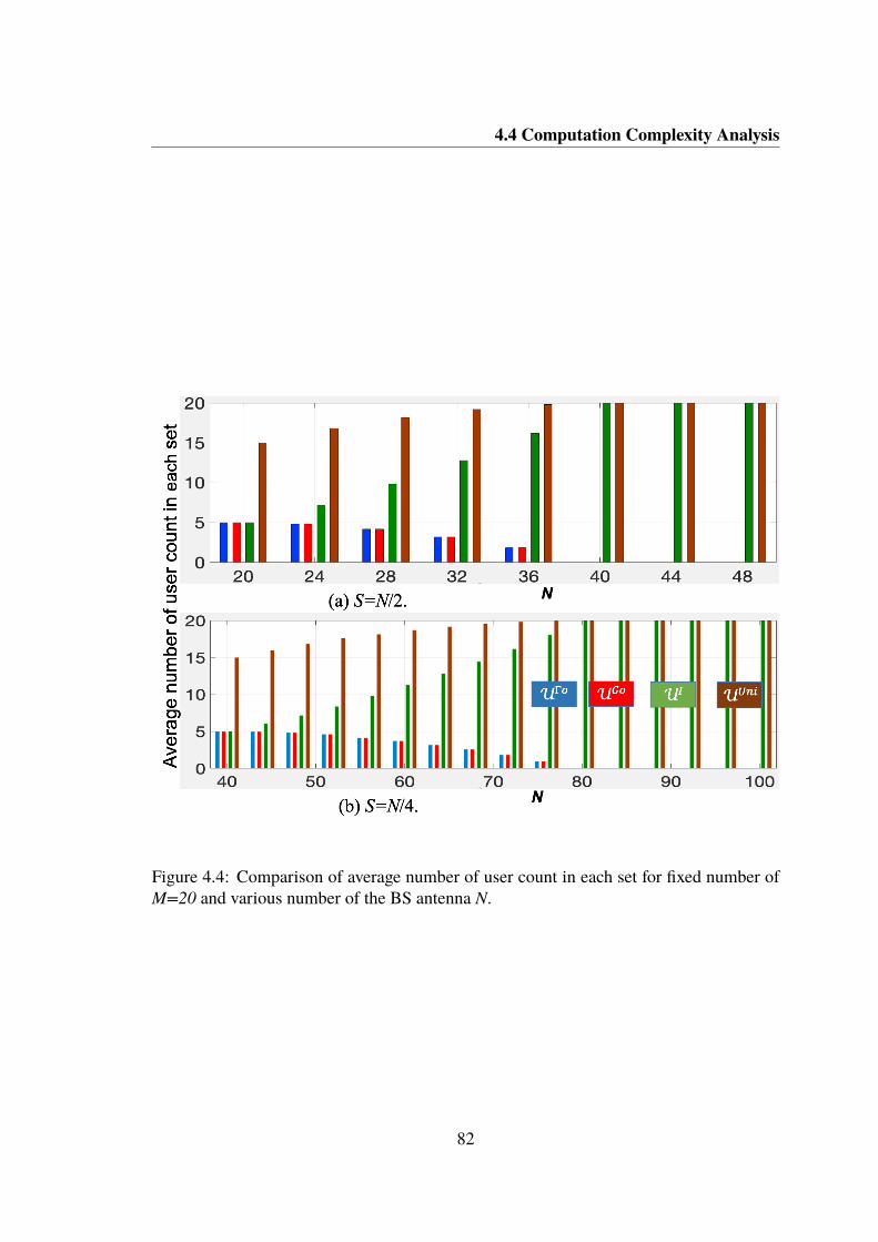
4.4 Computation Complexity Analysis
Figure 4.4: Comparison of average number of user count in each set for fixed number ofM=20 and various number of the BS antenna N.
82

4.4 Computation Complexity Analysis
it will cause more common users in the set UI . When N=40, RF will become 20, and S
will be equal to all the available users in the cell. Therefore, all users can be chosen to
serve, and common user set will be maximum after S=M . Although, a larger number of
N with S=N/4 are used in Fig. 4.4(b), we can see a similar situation as it was explained
in Fig. 4.4(a).
Figure 4.5: Comparison of possible combinations for the BFS search for fixed number ofM=20 and various number of the BS antenna N.
Figure 4.5(a) shows the number of possible combinations to use for the BFS for each
method. The total combinations of the proposed method will be gradually decreased from
N=20 to N=48 since results of (4.7) will influence for the total number of combinations.
When S is larger than the number of available users M , there is no need to do the user
selection part, and only the results of (4.5) will decide for a total number of combinations,
and it gives a little bit increase in total number of combinations for the BFS. A similar
83
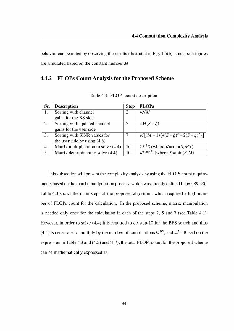
4.4 Computation Complexity Analysis
behavior can be noted by observing the results illustrated in Fig. 4.5(b), since both figures
are simulated based on the constant number M .
4.4.2 FLOPs Count Analysis for the Proposed Scheme
Table 4.3: FLOPs count description.
Sr. Description Step FLOPs1. Sorting with channel 2 4N M
gains for the BS side2. Sorting with updated channel 5 4M(S+ ζ)
gains for the user side3. Sorting with SINR values for 7 M[(M −1)4(S+ ζ)2+2(S+ ζ)2]
the user side by using (4.6)4. Matrix multiplication to solve (4.4) 10 2K2S (where K=min(S,M) )5. Matrix determinant to solve (4.4) 10 K log2(7) (where K=min(S,M)
This subsection will present the complexity analysis by using the FLOPs count require-
ments based on the matrix manipulation process, which was already defined in [60, 89, 90].
Table 4.3 shows the main steps of the proposed algorithm, which required a high num-
ber of FLOPs count for the calculation. In the proposed scheme, matrix manipulation
is needed only once for the calculation in each of the steps 2, 5 and 7 (see Table 4.1).
However, in order to solve (4.4) it is required to do step-10 for the BFS search and thus
(4.4) is necessary to multiply by the number of combinations ΩBS, and ΩU . Based on the
expression in Table 4.3 and (4.5) and (4.7), the total FLOPs count for the proposed scheme
can be mathematically expressed as:
84

4.4 Computation Complexity Analysis
FLOPsupper =ΩBSΩ
U(2K2S)(K log2(7))+4N M · · · i f M ≤ S. (4.8a)
FLOPsupper =ΩBSΩ
U(2K2S)(K log2(7))+4N M +4M(S+ ζ)
+M[(M −1)4(S+ ζ)2+2(S+ ζ)2] · · · i f M > S. (4.8b)
Figure 4.6: Comparison of FLOPs count for various number of total users M.
Figures 4.6 and 4.7 show the comparison of FLOPs count for proposed and conven-
tional methods. The slopes of the curves of the FLOPs count are similar to the total
number of combinations in Fig. 4.3 and Fig. 4.5 since the number of combinations is
the main influence factor for the complexity calculation in the selection scheme. FLOPs
counts expressed in (4.8) are upper bounds for the computation complexity, and the actual
computation complexity might not reach that upper bounds, since the BFS search may not
be required for some channel realizations.
85

4.5 Performance Evaluation, Results and Discussion
Figure 4.7: Comparison of FLOPs count for fixed number of M=20 and various numberof the BS antenna N.
4.5 Performance Evaluation, Results and Discussion
By using simulation parameters in Table 4.2, performances of schemes are compared in
terms of the CPU usage time and the sum-rate for the MU-Massive MIMO system under
consideration for the following four cases. The first one is increasing numbers of users M
with constant N and S. The second one is a stable numbered users M , and numbers of
antennas N and RF chains S increasing on the BS side for the given system. In addition,
two more set of performance results are obtained for the cases where S=N/2 and S=N/4.
CPU usage time for the calculation complexity results is normalized by using the smallest
value in each complexity performance figure to clarify the ratio of complexity for each
scheme.
Figure 4.8 shows the total sum-rate of the proposed system model. As ζ increases, the
proposed method can give more noticeable sum-rate improvement than methods in [47]
86
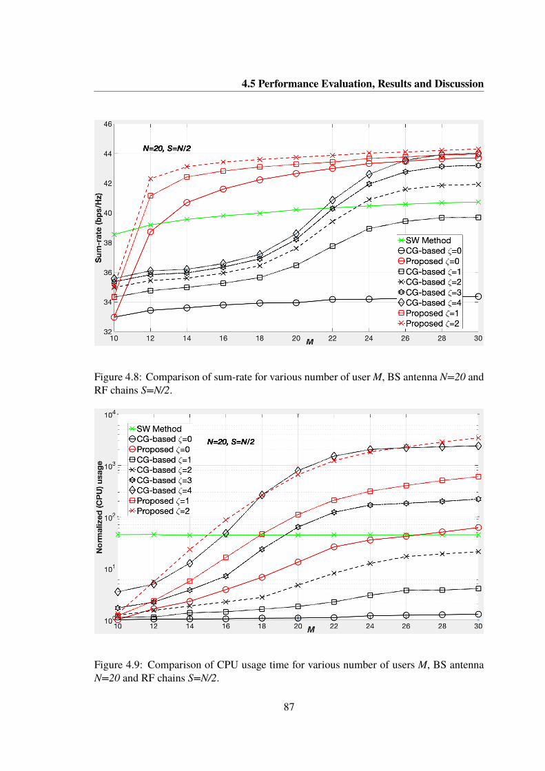
4.5 Performance Evaluation, Results and Discussion
Figure 4.8: Comparison of sum-rate for various number of user M, BS antenna N=20 andRF chains S=N/2.
Figure 4.9: Comparison of CPU usage time for various number of users M, BS antennaN=20 and RF chains S=N/2.
87

4.5 Performance Evaluation, Results and Discussion
and [83], especially for a moderate amount of user numbers in the cell. For M=S=10,
there is no user selection, and sum-rate improvement can be achieved only from transmit
antenna selection from the BS side. Therefore, no sum-rate improvement is possible for
the proposed method in the M=10 condition. However, when the number of users is
more considerable larger than available RF chains S in the system, significant sum-rate
improvement is achieved, as shown in Fig. 4.8. When M is much larger than S, the method
in [83] also achieves the distinguishable sum-rate improvement with more user diversity
in the system. On the other hand, the SW Method will give nearly flat conditions on the
sum-rate graph since their sum-rate improvement depends greatly on the transmit antenna
selection on the BS side with the sliding window method. Constant number N and RF
chain S will not support giving much more sum-rate improvement for SW method as
shown in Fig. 4.8.
Figure 4.9 shows the normalized CPU usage for each method. The proposed method
uses ζ = 0, 1 and 2 for the transmit antenna selection on the BS side. In contrast, the
method in [83] uses ζ = 0, 1, 2, 3, and 4 to control the computation complexity for the
transmit antenna selection on the BS side and receive user selection on the user side.
When a lower ζ value is applied to the method of [83], the CPU usage curves of ζ = 0, 1,
and 2 are lower than CPU usage curves of the proposed method. Little amount of the BFS
is necessary to do for the small number of possible combinations in transmit antenna set
and receive user set.
At that time, the proposed method has an overhead usage of CPU time for two sortings
on the user side. The proposed scheme is necessary to do not only for the CG computation
but also for the SINR computation to find the CG-based sorted user set UGsort and
the SINR-based sorted user set UΓsort for receive user selection. Although, this SINR
computation is not necessary to use SVD, this overhead SINR calculation gives a higher
88

4.5 Performance Evaluation, Results and Discussion
impact than a small amount of the BFS. However, the value of ζ becomes larger, this will
increase the computation complexity in the BFS for the possible combination of transmit
antennas and receive user sets. Therefore, the method in [83] gives more CPU usage for
the higher value of ζ . On the other hand, the SW Method provides the nearly constant
value of CPU usage all over the numbers of M since numbers of the BS antenna N and RF
chains S are always constant in this simulation. The SW Method uses sliding windows and
the number of windows depends on the available BS transmit antenna N , and RF chains
S. Therefore, it gives nearly constant value of CPU usage in Fig. 4.9.
Figure 4.10: Comparison of sum-rate for various number of users M, BS antenna N=40and RF chains S=N/4.
Figures 4.8 and 4.10 show the sum-rate improvement of S = N/2 (S = 50% of N) and
S = N/4 (S = 25% of N) conditions for each method. Both the proposed and CG-based
methods have same preselection steps for the transmit antenna selection case on the BS
side. In step-4, AGpre is created based on qA which can be obtained in step-3. When S
89

4.5 Performance Evaluation, Results and Discussion
Figure 4.11: Comparison of CPU usage time for various number of users M, BS antennaN=40 and RF chains S=N/4.
is constant (S = 10 in both figures), a smaller number of N will give a lower qA value,
and the larger number of N will give a higher qA. Lower qA will give the lower number
of preselected transmit antenna elements in AGpre set, and higher qA will give the larger
AGpre according to the conditional statements in step-4. If AGpre is large, we have more
chance to choose the best transmit antennas set by using the BFS search in step-10, and this
will give more sum-rate improvement for larger number of N . Since AGpre in Fig. 4.10 is
larger than AGpre in Fig. 4.8, and this will lead higher sum-rate improvement.
For the user selection part in the proposed method, the number of preselected users
in the UGpre and UΓpre sets are not affected by the number of transmit antennas on the
BS side as shown in Fig. 4.2. For the same user number in Fig. 4.8 and Fig. 4.10 (e.g.,
M=12), extra sum-rate improvement of the proposed method is achieved mainly from the
90

4.5 Performance Evaluation, Results and Discussion
transmit antenna selection on the BS side. And the sum-rate plots of the proposed scheme
have the similar slopes for each M in both figures.
On the other hand, the CG-based method used the same preselection concept for the BS
and user side [83]. When number of user M is not considerably larger than the number of
RF chains S, the CG-based method will produce a small preselected user set UGpre under
the limitation of qU. qU is the number of users which CGs are larger than the mean CG
[83]. It will cause the lower number of combinations in the BFS search, and give a slight
sum-rate improvement from the user side. When M is lower than 20, not as much sum-rate
improvement can be achieved from the UGpre set in both figures. Therefore, AGpre will
influence mainly for the lower number of M , and this gives the sum-rate improvement at
the condition of lower M (M < 20) for the CG-based method in Fig. 4.8 and Fig. 4.10.
When the number of users is gradually increased, more user elements are assigned in
UGpre and higher chance to select the best users from the larger UGpre. Therefore, the
noticeable increasing sum-rate can be seen between M=20 to 26 for the CG-based method.
When the number of users M is much larger than RF chain S, the maximum size of UGpre
is limited by (S + ζ) and UGpre will be gradually situated. The situated UGpre cannot
give a more significant sum-rate improvement for larger user numbers M in Fig. 4.8 and
Fig. 4.10.
Figures 4.10 and 4.11 compare the performances of S=N/4 case with N=40 for various
numbers of M . When N is much larger than S, extra sum-rate improvement comes from
more diversity and freedom of transmit antenna selection on the BS side. This benefit
can be seen not only in the proposed method but also in other methods. The CG-based
method shows distinguish sum-rate improvement with extra computation complexity as
shown in Fig. 4.10 and Fig. 4.11. The proposed method has the same condition of user
selection parts since numbers of user distribution in the sets UΓo, UGo, UI and UUni are
91

4.5 Performance Evaluation, Results and Discussion
not much different with the S=N/2 case. For the selection scheme in the SW Method,
all of the available antenna elements on the BS side are considered by using the sliding
window method. Therefore, this method also gives nearly constant value of sum-rate and
CPU usage for constant value of N in the figure.
Figure 4.12: Comparison of sum-rate for various number of the BS antenna N and RFchains S=N/2, with total users M=20.
Figures 4.12 to 4.15 compare the performances of each method. As presented and
explained in Fig. 4.4, the number of user count in the sets UΓo, UGo is gradually decreased
until S is approximately equal to M . The computation complexity also depends on the
size of sets UΓo, UGo as stated in (4.7). Therefore, decreasing the size of sets UΓo, UGo
will give fewer possible combinations and this will cause a reduction in computation
complexity in the selection scheme. Moreover, the number of elements in the sets UI
is gradually increased for increasing number of N . This condition gives less number of
outcome for the possible combinations in (4.7). Therefore, we can obtain the reduction of
92

4.5 Performance Evaluation, Results and Discussion
Figure 4.13: Comparison of CPU usage time for various number of the BS antenna N andRF chains S=N/2, with total users M=20.
Figure 4.14: Comparison of sum-rate for various number of the BS antenna N and RFchains S=N/4, with total users M=20.
93

4.5 Performance Evaluation, Results and Discussion
Figure 4.15: Comparison of CPU usage time for various number of the BS antenna N andRF chains S=N/4, with total users M=20.
computation complexity of the proposed method as shown in Fig. 4.13. The conventional
SW Method gradually increases the computation complexity since it is necessary to
use SVD calculation for more number of sliding windows on the BS side to find the
best transmit antenna set. The method in [83] gives decreasing pattern of computation
complexity when number of S is approached to M . In that condition, the user selection
is not necessary to do the full combination search, because the available RF chain is
approached to the total user number in a cell. The computation complexity from the
user side is eventually diminished for increasing number of S. However, when S is larger
than total user M then the total sum-rate and computation complexity of the proposed
method and CG-based method will be overlapped since there has no more user selection is
included in both methods. The constant increment of sum-rate improvements in Fig. 4.12
and Fig.4.14 come from the constant increment of transmit antenna N and RF chains S.
94

4.6 Summary of Contribution in MU-Massive MIMO System
However, the proposed method can give higher sum-rate than conventional methods from
a smaller number of transmit antenna to a larger number of transmit antenna case. This
improvement can be achieved mainly from the user side selection part. When number of
RF chains S is approached to M , no more user diversity is achieved and the sum-rate of
the proposed method will be overlapped with the method in [83].
4.6 Summary of Contribution in MU-Massive MIMOSystem
We have presented the combined method of CG-based and SINR-based receive user selec-
tion schemes for the downlink MU-Massive MIMO TDD system with BD transmission.
The proposed scheme can reduce the computation complexity of antenna/user selection
while improving sum-rate performance in the system, especially for the system parameters
when the number of user M is not much larger than available RF chains S. When M
is much larger than S, the user diversity is more than enough and the sum-rate improve-
ment of the proposed scheme is not much obvious when compared with the conventional
schemes.
95

Chapter 5
Conclusion
In this dissertation, we presented our research works on promises technologies for next
generation broadband wireless mobile communication systems. In Chapter 1, history and
evolution of mobile wireless generation are presented in first and after that, the back ground
information and theories of OFDM/OFDMA, MIMO, antenna and user selection methods
are introduced. MIMO technologiy can be categorized as SU-MIMO, MU-MIMO and
Massive MIMO. MIMO technologies can give the high speed internet access under the
limited resources of radio frequency without additional transmit power in the wireless
system. MIMO technology in spectral multiplexing system will work more efficiently if
there has rich scattering multipath channel environment to give the low correlated channel
matrix in the system. Therefore, our research works focused on this MIMO technologies in
spatial multiplexing system for higher data transfer rate in next generation mobile wireless
system.
When a BS is equipped with a large number of antennas (e.g. tens or hundreds) and
communicates with several single-antenna users in the same time-frequency domain, then
this system can be known as Massive MIMO [18]. The increasing capacity results from
aggressive spatial multiplexing used in the Massive MIMO. The basic premise behind
the Massive MIMO is to reap all of the benefits of the conventional MIMO, but on
96

much greater scale. It has been shown that the large antenna array at BS could provide
high degrees of freedom and thus increase significantly the system capacity, the link
reliability, and the radiated-energy efficiency. Also, based on the random matrix theory,
it was demonstrated that the Massive MIMO system could achieve the capacity gain with
simple and linear signal processing methods. However, number of RF chains at the BS
cannot be large very much due to the constraints in hardware cost and the complexity for
practical system. Adding more antennas at the BS is usually inexpensive. However, the RF
elements, such as RF chains can be relatively expensive. Therefore, most Massive MIMO
systems should consider to implement the BS with larger number of antenna elements
but fewer number of RF chains to reduce the hardware cost in the BS side. Since all
antennas are not equally good in real propagation channels, it is possible to reduce RF
chains to be used with selected active antennas, which contribute the most in the system
performance and discarding the rest of antennas. Such antenna selection could simplify
the design of a Massive MIMO base station and lead to energy and cost savings. In this
case, selecting and using the best antennas among the available large number of antenna
elements in BS is an important issue in Massive MIMO technology. Massive MIMO
equipped with a large number of antennas at the BS can communicate with multiple
users simultaneously. Simultaneous communication with multiple users creates multiuser
interference and degrades the throughput performance. Precoding methods are applied
during the downlink to reduce the effect of multiuser interference. Since the number of
antennas is limited in Massive MIMO base station, if the number of users becomes more
than the number of antennas, proper user selection scheme is applied before precoding
to achieve higher throughput and sum rate performance. Therefore, the user selection
is also a critical important factor for optimizing the overall performance of Massive
MIMO systems. Antenna selection and user selection in the multi user Massive MIMO
97

systems have been widely studied as presented in above, but all of them consider only for
antenna selection in the BS side or the user selection in the user side. To the best of our
knowledge, there are only few studies on joint antenna selection for MU-Massive MIMO
systems. Therefore, we emphasized to do the research works on finding of antenna and
user selection in Massive MIMO system.
In this dissertation, I presented the low complexity joint antenna and user selection
scheme for the downlink MU massiveMIMOTDD system in Chapter 3. To achieve the
reduced complexity in the antenna and user selection while maintaining the same or
higher sum-rate in the system, the proposed scheme relies on three complexity reduction
key factors. The first key factor is that finding the average CGs for the transmit antenna
in the BS side and the receive antenna in the user side to select the best CG antennas
and users. The second key factor called the complexity control for the antenna set and
the user set limitation is used to control the complexity of brute force search. The third
one is that using the assumption of point-to-point deterministic MIMO channel model to
avoid the SVD computation in brute force search. The numerical complexity analysis is
also used to compare the lower and upper bound of the proposed scheme with the optimal
and sliding window based scheme. It can be seen that lower bound of the proposed
scheme is always lower than other two schemes and we can use the various value to
control the complexity in the proposed schemes. Moreover, simulation results show that
the proposed scheme outperforms the two conventional methods in the CPU usage time
while maintaining the same or higher sum-rate in most of the scenarios of the MU-Massive
MIMO communication. When number of RF chains is large enough to compare with the
half of the number of users or the BS antenna in the system, the proposed scheme faces
the restricted condition to choose the better SINR user to create the good transmit antenna
98

set and receive user set in the system. This will cause lower sum-rate in some particular
cases.
A novel user selection scheme which is based on the previous research work are pre-
sented in Chapter 4. The proposedd novel selection scheme is a combined method of
CG-based and SINR-based receive user selection schemes for the downlink MU-Massive
MIMO TDD system with BD transmission. The proposed scheme can reduce the com-
putation complexity of antenna/user selection while improving sum-rate performance in
the system, especially for the system parameters when the number of user M is not much
larger than available RF chains S. When M is much larger than S, the user diversity is more
than enough and the sum-rate improvement of the proposed scheme is not much obvious
when compared with the conventional schemes.
As an overall conclusion, this dissertation contributes the antenna and user selection
schemes with exact fulfilment of low computational complexity requirement for downlink
MU-Massive MIMO system. Noticeable data sum-rate improvements are also achieved
in the system.
In future extension of our research, we will consider to develop the selection schemes
for various wireless environments such as multi-cell, Rician fading etc. For Rician fading
environment CG-based selection method might select users which cannot give higher
data sum-rate when compared with Rayleigh fading environment. As already discussed
in Chapter 2, CG-based selection method will choose users with highest channel gains
with no consideration of interference effects of nearby users. This kind of selectin give
low sum-rate results in the system. If user distribution in the cell is more scatter in the
Rician fading environment, the proposed method might have more common users in the
preselection stage and it will give more computation complexity reduction. Therefore, we
99

should do research for different levels of user distributions in the cell to compare data sum-
rate and complexity results for CG-based and the proposed methods. It is also possible
to develop the antenna and user selection schemes for multi-cell environment with both
uplink and downlink communication. When multi-cell environment is considered, one
should carefully examine about imperfect CSI because of neighburing cells if there has no
co-operation from those neighbouring cells in the system. Because of imperfect CSI and
interference from the neighbouring cells, joint consideration of CG-based and SINR-based
selection might have superior performance than CG only based selection scheme in the
system. When uplink communication is considered in the system, we can expect similar
sum-rate performance improvements like downlink communication for TDD system since
uplink communication is the reciprocal of downlink communication in the MU-Massive
MIMO system.
100

Bibliography
[1] K. L. Corum and J. F. Corum. "Nikola Tesla and the Planetary Radio Signals".
[2] "Brief History of Wireless Communications". https://www.carritech.com/news/
brief-history-wireless-communications, . Access at 1 July 2021.
[3] "Cisco Annual Internet Report". https://www.cisco.com/c/en/us/solutions/collateral/
executive-perspectives/annual-internet-report/white-paper-c11-741490.html, .
White Paper (2018-2023).
[4] A. F. Molish, V. V. Ratnam, S. Han, Z. Li, and K. Haneda. "Hybrid Beamforming
for Massive MIMO A Survey". IEEE Commun. Mag., 5(5):134–141, July 2017.
[5] B. Yang, Z. Yu, J. Lan, R. Zhang, J. Zhou, and W. Hong. "Digital Beamforming-
Based Massive MIMO Transceiver for 5G Millimeter-Wave Communications". IEEE
Trans. Microw. Theory., 66(5):3403–3418, Jun 2018.
[6] A. Paulraj and T. Kailath. "Increasing Capacity in Wireless Broadcast Systems Using
Distributed Transmission/Directional Reception". (5 345 599), Sep 1994.
[7] G.J. Foschini and M.J. Gans. "On Limits of Wireless Communications in a Fading
Environment When Using Multiple Antennas". In Wireless Pers. Commun, pages
311–335, Jun 1998.
101

BIBLIOGRAPHY
[8] Q.H. Spencer, C.B. Peel, A.L. Swindlehurst, and M. Haardt. "An Introduction to
MIMO Channels". In IEEE Commun. Mag., volume 42, pages 60–67, 2004.
[9] A. Kurve. "Multiuser MIMO Systems: The Future in the Making". In IEEE
Potentials., volume 28, pages 37–42, 2009.
[10] D. Nojima, L. Lanante, Y. Nagao, M. Kurosaki, and H. Ochi. "Performance Eval-
uation for Multiuser MIMO IEEE 802.11ac Wireless LAN System". In Intl. Conf.
on Advanced Communication Technology (ICACT),, volume 14, pages 804–808, Feb
2012.
[11] M. Jiang and L. Hanzo. "Multiuser MIMO-OFDM for Next-Generation Wireless
Systems". In IEEE, volume 95, pages 1430–1469, 2007.
[12] P. W. Wolniansky, G. J. Foschini, G. D. Golden, and R. A. Valenzuela. "V-BLAST:An
Architecture for Realizing Very High Data Rates Over the Rich-scattering Wireless
Channel". In Proc. IEEE ISSSE, Sep 1998.
[13] I. E. Telatar. "Capacity of Multi-Antenna Gaussian Channels". In AT & T Bell
Laboratories Tech. Rep.
[14] H. Winters. "Optimum Combining in Digital Mobile Radio with Co-channel Inter-
ference". IEEE J. Sel. Areas Commun., 2(4):528–539, July 1984.
[15] S. Anderson, M. Millnert, M. Viberg, and B. Wahlberg. "An Adaptive Array for
Mobile Communication Systems". IEEE Trans. Veh. Technol, 40(1):230–236, Feb
1991.
[16] A. Gold Smith, S. A. Jafar, N. Jindal, and S. Vishwanath. "Capacity Limits of MIMO
Channels". IEEE J. Sel. Areas Commun, 21(5):684–702, June 2003.
102

BIBLIOGRAPHY
[17] D. Gesbert, M. Kountouris, R.W. Heath, Jr. C.B. Chae, and T. Salzer. "From Single-
User to Multi-User Communiications: Shifting the MIMO Paradigm". IEEE Signal
Process. Mag, 24(5):36–46, Sep 2007.
[18] T. L. Marzetta, G. E. Larsson, H. Yang, and H. Q. Ngo. "Fundamentals of Massive
MIMO". In Cambridge University Press, 2016.
[19] T.L. Marzettta. "How Much Training is Required for Multiuser MIMO?". In Proc.
40th Asilomar Conf. on Signals, Systems and Computers (ACSSC), Nov 2006.
[20] T.L. Marzetta. "Noncooperative Cellular Wireless with Unlimited Numbers of Base
Station Antennas". IEEE Trans. Wireless Commun., 9(11):3590–3600, Feb 2010.
[21] G. E. Larsson, O. Edfors, F. Tufvesson, and T. L. Marzetta. "Massive MIMO for
Next Generation Wireless Systems". IEEE Trans. Commun. Mag., 52(2):186–195,
Feb 2014.
[22] T. L. Marzetta. "Massive MIMO: An Introduction". In Bell Labs Tech. J., volume 20,
pages 11–22, 2015.
[23] N.H.M. Adnan, I.M. Rafiqul, and A.H.M.Z Alam. "Massive MIMO for Fifth Gen-
eration (5G): Opportunities and Challenges.". In Proc. of the 2016 Intl. Conf. on
Computer and Communication Engineering (ICCCE), pages 47–52, July 2016.
[24] E. Bjrnson, J. Hoydisn, and L. Sanguinetti. "Massive MIMO Networks: Spectral,
Energy, and Hardware Efficiency". In Trends Signal Proc, volume 11, pages 154–
165, 2017.
[25] "A Closer Look at Massive MIMO". https://business.sprint.com/blog/massive-
mimo, . Accessed at 1 July 2021.
103

BIBLIOGRAPHY
[26] F. Rusek, D. Persson, B. K. Lau, E. Larsson, T. Marzetta, O. Edfors, and F. Tufvesson.
"Scaling Up MIMO: Opportunities and Challenges with Very Large Arrays". IEEE
Signal Process. mag., 30(1):40–60, Jan 2013.
[27] E. Bjrnson, E.G. Larsson, and T. L. Marzetta. "Massive MIMO: Ten Myths and One
Critical Question". In IEEE Commun. Mag, volume 54, pages 114–123, 2016.
[28] T. Van Chien and E. Bjrnson. "Massive MIMO Communications in 5G Mobile
Communications". In Springer, pages 77–116, 2017.
[29] "5G Researchers Set New World Record For Spectrum Efficiency".
https://spectrum.eee.org/tech-talk/telecom/wireless/5g-researchers-achieve-new-
spectrum-efficiency-record, . Accessed at 1 July 2021.
[30] S. Malkowsky, J. Vieira, L. Liu, P. Harris, K. Nieman, N. Kundargi, I. C.Wong,
F. Tufvesson, V. Wall, and O. Edfors. "The Worlds First Real-Time Test-bed for
Massive MIMO: Design, Implementation, and Validation". IEEE Access, (5):9073–
9088, 2017.
[31] R. Chataut and R. Akl. "Massive MIMO Systems for 5G and Beyond Networks
Overview, Recent Trends, Challenges, and Future Research Direction". Sensor J.,
May 2020.
[32] L. Lu, G. Y. Li, A. L. Swindlehurst, A. Ashikhmin, and R. Zhang. "An Overview
of Massive MIMO: Benefits and Challenges". IEEE J. Sel. Top. Signal Proc, (8):
742–758, 2014.
104

BIBLIOGRAPHY
[33] J. Jose, A. Ashikhmin, T. L. Marzetta, and S. Vishwanath. "Pilot Contamination
and Precoding in Multi-cell TDD Systems". IEEE Trans. Wireless Commun, (10):
2640–2651, 2011.
[34] B. Gopalakrishnan and N. Jindal. "An Analysis of Pilot Contamination on Multi-
user MIMO Cellular Systems with Many Antennas". In Proc. of the IEEE 12th
Intl. Workshop on Signal Process. Advances in Wireless Communications (SPAWC),
pages 381–385, Jun 2011.
[35] N. Krishnan, R. Yates, and N. Mandayam. "Cellular Systems with Many Antennas:
Large System Analysis under Pilot Contamination". In Proc. of the 50th Annual
Allerton Conf. on Communication, Control, and Computing (Allerton), pages 1220–
1224, Oct 2012.
[36] M.A.M. Moqbel, W. Wangdong, and A. Z. Ali. "MIMO Channel Estimation Using
the LS and MMSE Algorithm". Electron. Commun. Eng, (12):13–22, 2017.
[37] X. Wu, L. Gu, W. Wang, and X. Gao. "Pilot Design and AMP-based Channel Esti-
mation for Massive MIMO-OFDM Uplink Transmission". In Proc. of the 2016 IEEE
27th Annual Intl. Symposium on Personal, Indoor, and Mobile Radio Communica-
tions (PIMRC), pages 1–7, Sep 2016.
[38] N. Fatema, G. Hua, Y. Xiang, D. Peng, and I. Natgunanathan. "Massive MIMO
Linear Precoding: A Survey". IEEE Syst. J., (12):3920–3931, 2018.
[39] J. Hoydis, S. ten Brink, and M. Debbah. "Massive MIMO in the UL/DL of Cellular
Networks: How Many Antennas Do We Need?". IEEE J. Sel. Areas Commun., 31
(2):160–171, Feb 2013.
105

BIBLIOGRAPHY
[40] L. Lu, G. Li, A. Swindlehurst, A. Ashikhmin, and R. Zhang. "An Overview of
Massive MIMO: Benefits and Challenges". IEEE J. Sel. Topics Signal Process., 8
(5):742–758, Oct 2014.
[41] X. Gao, O. Edfors, J. Liu, and F. Tufvesson. "Antenna Selection in Measured Massive
MIMO Channels Using Convex Optimization". In Second Intl. Conf. on Advanced
Computing Communication Technologies, pages 535–541, Jan 2012.
[42] M. Benmimoune, E. Driouch, and W. Aji. "Joint Antenna Selection and Grouping in
Massive MIMO systems". In 10th Intl. Symposium on Commun., Systems, Networks
and Digital Signal Process. (CSNDSP), Prague, Czech Republic, July 2016.
[43] H. Liun, H. Gao, S. Yang, and T. Lv. "Low-Complexity Downlink User Selection
for Massive MIMO Systems". IEEE Sys. J., 11(2):1072–1083, May 2015.
[44] G. Lee and Y. Sung. "Asymptotically Optimal Simple User Scheduling for Massive
MIMO Downlink with Two-Stage Beamforming". In Int. Workshop Signal Process.
Adv. Wireless Commun., pages 1–5, June 2014.
[45] Y. Xu, G. Yue, and S. Mao. "User Grouping for Massive MIMO in FDD Systems:
New Design Methods and Analysis". IEEE Access, 2:947–959, Aug 2014.
[46] G. Xu, A. Liu, W. Jiang, H. Xiang, and W. Luo. "Joint User Scheduling And Antenna
Selection in Distributed Massive MIMO Systems with Limited Backhaul Capacity".
In China Commun, pages 17–30, May 2014.
[47] Moo-Woong Jeong, Tae-Won Ban, and Bang Chul Jung. "User and Antenna Joint
Selection in Multi-User Large-Scale MIMO Downlink Networks". IEICE Trans.
Commun, E100-B:529–535, Apr 2017.
106
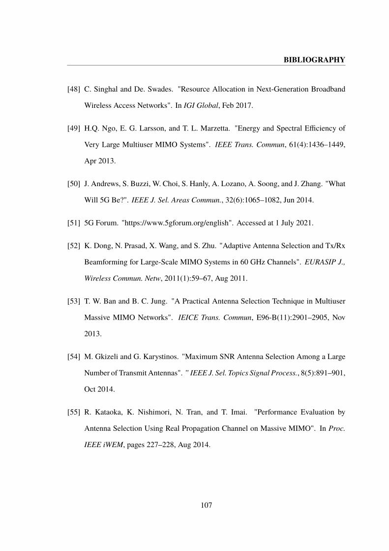
BIBLIOGRAPHY
[48] C. Singhal and De. Swades. "Resource Allocation in Next-Generation Broadband
Wireless Access Networks". In IGI Global, Feb 2017.
[49] H.Q. Ngo, E. G. Larsson, and T. L. Marzetta. "Energy and Spectral Efficiency of
Very Large Multiuser MIMO Systems". IEEE Trans. Commun, 61(4):1436–1449,
Apr 2013.
[50] J. Andrews, S. Buzzi, W. Choi, S. Hanly, A. Lozano, A. Soong, and J. Zhang. "What
Will 5G Be?". IEEE J. Sel. Areas Commun., 32(6):1065–1082, Jun 2014.
[51] 5G Forum. "https://www.5gforum.org/english". Accessed at 1 July 2021.
[52] K. Dong, N. Prasad, X. Wang, and S. Zhu. "Adaptive Antenna Selection and Tx/Rx
Beamforming for Large-Scale MIMO Systems in 60 GHz Channels". EURASIP J.,
Wireless Commun. Netw, 2011(1):59–67, Aug 2011.
[53] T. W. Ban and B. C. Jung. "A Practical Antenna Selection Technique in Multiuser
Massive MIMO Networks". IEICE Trans. Commun, E96-B(11):2901–2905, Nov
2013.
[54] M. Gkizeli and G. Karystinos. "Maximum SNR Antenna Selection Among a Large
Number of Transmit Antennas". ” IEEE J. Sel. Topics Signal Process., 8(5):891–901,
Oct 2014.
[55] R. Kataoka, K. Nishimori, N. Tran, and T. Imai. "Performance Evaluation by
Antenna Selection Using Real Propagation Channel on Massive MIMO". In Proc.
IEEE iWEM, pages 227–228, Aug 2014.
107

BIBLIOGRAPHY
[56] X. Gao, O. Edfors, F. Tufvesson, and E. G. Larsson. "Massive MIMO in Real
Propagation Environments: Do All Antennas Contribute Equally?". IEEE Trans.
Commun, 63(11):3917–3928, Jul 2015.
[57] M. Benmimoune, E. Driouch, W. Ajib, and D. Massicotte. "Joint Transmit Antenna
Selection and User Scheduling for Massive MIMO Systems". In Proc. IEEE WCNC,
pages 381–386, Mar 2015.
[58] J. C. Chen. "Joint Antenna Selection and User Scheduling for Massive Multiuser
MIMO Systems With Low-Resolution ADCs". IEEE Trans.Vehicular Tech, 68(1):
1019–1024, Jan 2019.
[59] Q. H. Spencer, A. L. Swindlehurst, and M. Haardt. "Zero-forcing Methods for
Downlink Spatial Multiplexing in Multiuser MIMO Channels". IEEE Trans. Signal
Process., 52(2):461–471, Feb 2004.
[60] Z. Shen, R. Chen, J. Andrews, R. Heath, and B. Evans. "Low Complexity User
Selection Algorithms for Multiuser MIMO Systems with Block Diagonalization".
IEEE Trans. Signal Process., 54(9):3658–3663, Sep 2006.
[61] S. Sandhu, R. Nabar, D. Gore, and A. Paulraj. "Near-Optimal Selection of Transmit
Antennas for a MIMO Channel Based on Shannon Capacity". In Asilomar Conf.
Signals, Syst. Comput., Pacific Grove, Nov 2000.
[62] R. W. Heath Jr., S. Sandhu, and A. Paulraj. "Antenna Selection for Spatial Multi-
plexing Systems with Linear Receivers". IEEE Commun. Lett., 5(2):142–144, Apr
2001.
108

BIBLIOGRAPHY
[63] D. Gore, R. W. Heath Jr., and A. Paulraj. "Transmit Selection in Spatial Multiplexing
Systems". IEEE Commun. Lett., 6(11):491–493, Nov 2002.
[64] R. Chen, J. Andrews, and R. W. Heath Jr. "Efficient Transmit Antenna Selection
for Multiuser MIMO Systems with Block Diagonalization". In Proc. IEEE Global
Telecommun., Washington, DC, USA, Nov 2007.
[65] H. A. Seleh and W. Hamouda. "Transmit Antenna Selection for Decision Feedback
Detection in MIMO Fading Channels". IEEE Trans. Wireless. Commun., 8:4440–
4444, Sep 2009.
[66] O. Mehanna, N. D. Sidiropoulos, and G. B. Giannakis. "Joint Multicast Beamforming
and Antenna Selection". IEEE Trans. Signal Process., 61:2660–2674, May 2013.
[67] S. Khademi, S. Chepuri, G. Leus, and A. J. V. D. Veen. "Zero-Forcing Pre-
Equalization with Transmit Antenna Selection in MIMO Systems". In Proc. IEEE Int.
Conf. Acoust., Speech Signal Process., Vancouver, BC, Canada, pages 5043–5050,
May 2013.
[68] H. Li, L. Song, and M. Debbah. "Energy Efficiency of Large-Scale Multiple Antenna
Systems with Transmit Antenna Selection". IEEE Trans. Commun., 62(2):638–647,
Feb 2014.
[69] Y. Yu, H. Chen, Y. Li, Z. Ding, L. Song, and B. Vucetic. "Antenna Selection for
MIMO Nonorthogonal Multiple Access Systems". IEEE Trans. Veh. Technol., 67
(4):3158–3171, Apr 2018.
109

BIBLIOGRAPHY
[70] M. Ahn, H. Kong, H. M. Shin, and I. Lee. "A Low Complexity User Selection
Algorithm for Full-Duplex MU-MISO Systems". IEEE Trans. Wireless Commun.,
15(11):7899–7907, Nov 2016.
[71] S. Yu, J. Koh, and J. Kang. "Design of User Selection Algorithm in Fullduplex
Cellular System". In Proc. 14th IEEE Annu. Consumer Commun. Netw. Conf, pages
922–927, Jan 2017.
[72] Sanayei and A. Nosratinia. "Antenna Selection in MIMO Systems". ” IEEE Commun.
Mag, pages 68–73, Oct 2004.
[73] M. Gharavi-Alkhansari and A. Gershman. "Fast Antenna Subset Selection in MIMO
Systems". IEEE Trans. Sig. Proc, 52:339–347, 2004.
[74] Y. S. Choi, A.F. Molisch, M.Z. Win, and J.H. Winters. "Fast Algorithms for Antenna
Selection in MIMO Systems". In Proc. VTC, pages 1733–1737, July 2003.
[75] G. T. Chyi, J. G. Proakis, and C. M. Keller. "On the Symbol Error Probability of
Maximum Selection Diversity Reception Schemes Over a Rayleigh Fading Channel".
IEEE Trans. Commun, pages 79–83, Jan 1989.
[76] E. A. Neasmith and N. C. Beaulieu. "New Results on Selection Diversity". IEEE
Trans. Commun, 46:695–704, May 1998.
[77] D. A. Gore and A. Paulraj. "Space Time Block Coding with Optimal Antenna
Selection". In Proc. IEEE ICASSP, pages 2441–2444, May 2001.
[78] D. A. Gore and A. Paulraj. "MIMO Antenna Subset Selection with Space-Time
Coding". IEEE Trans. Signal Process., 50:2580–2588, Oct 2002.
110

BIBLIOGRAPHY
[79] A. Gorokhov. "Antenna Selection Algorithms for MEA Transmission Systems". In
Proc. IEEE ICASSP, pages 2857–2860, May 2002.
[80] Y. S. Cho, J. Kim, W. Y. Yang, and C. G. Kang. "MIMO-OFDM Wireless Com-
munications with MATLAB,". In John Wiley and Sons, number ISBN:0470825626,
pages 383–393, Aug 2010.
[81] M. S. Maw and S. Iwao. "Reduced Complexity in Antenna Selection for Polar-
ized MIMO System with SVD for the Practical MIMO Communication Channel
Environment". IEICE Trans. on Commun., E93-B(9):2389–2399, Sep 2010.
[82] M. S. Maw and S. Iwao. "Resource Allocation Scheme in MIMO-OFDMA System
for User’s Different Data Throughput Requirements". IEICE Trans. on Commun.,
E91-B(2):494–504, Feb 2008.
[83] A. M. Htun, M. S. Maw, and S. Iwao. "Low-Complexity Joint Antenna and User Se-
lection Scheme for the Downlink Multiuser Massive MIMO System with Complexity
Reduction Factors". IEICE Trans. Commun, E102-B(3):592–602, Mar 2019.
[84] H. P. Nik. "Introduction to Probability, Statistics, and Random Processes". In
Amazon, Kappa Research LLC, Aug 2014.
[85] G. Dirmic and N. D. Sidiropoulos. "On Downlink Beamforming with Greedy User
Selection: Performance Analysis and a Simple New Algorithm". IEEE Trans. Signal
Process., 53(10):3857–3868, Oct 2005.
[86] T. Yoo and A. Goldsmith. "On the Optimality of Multi-Antenna Broadcast Scheduling
Using Zero-Forcing Beamforming". IEEE J. Select. Areas Commun, 24(3):528–541,
Mar 2006.
111

BIBLIOGRAPHY
[87] A. Paulraj, R. Nabar, and D. Gore. "Introduction to Space-Time Wireless Commu-
nications". In Cambridge University Press, 2003.
[88] Z. Shen, R. Chen, J. Andrews, R. Heath, and B. Evans. "Low Complexity User
Selection Algorithms for Multiuser MIMO Systems with Block Diagonalization".
IEEE Trans. Signal Process., 54(9):3658–3663, Sep 2006.
[89] G.H. Golub and C.F. Van Loan. "Matrix Computations". In John Hopkins Press.
[90] Q. Alfio, S. Fausto, and G. Paola. "Scientific Computing with MATLAB and Octave".
In Springer, May 2010.
[91] G. Tsoulos. "MIMO System Technology for Wireless Communications". In CRC
Press, 2006.
112

Appendix A
Publication List
A.1 Journals
1. Aye Mon Htun, Maung Sann Maw, Iwao Sasase, “Low-Complexity Joint Antenna
and User Selection Scheme for the Downlink Multiuser Massive MIMO System with
Complexity Reduction Factors, ” IEICE Trans Communications., Vol. E102-B No.3,
pp.592-602, Mar. 2019.
2. Aye Mon Htun, Maung Sann Maw, Iwao Sasase, “A Novel Low Complexity Scheme for
Multiuser Massive MIMO Systems, ” IEICE Trans Communications., Vol. E105-B,No.1,
pp.-, Jan. 2022.
A.2 Articles on international conference proceedings (peer-reviewed full-length papers)
1. Aye Mon Htun, Maung Sann Maw, Iwao Sasase,“Reduced Complexity on Mobile
Sensor Deployment and Coverage Hole Healing by Using Adaptive Threshold Distance
in Hybrid Sensor Networks, ” on 25th IEEE Personal Indoor and Mobile Radio Commu-
nications (IEEE PIMRC 2014) Washington. DC, USA, September 2014.
2. Aye Mon Htun, Maung Sann Maw, Iwao Sasase, “Relocation of Mobile Sensor Nodes
113

A.3 Other international conference papers (full-length papers)
with Battery Aware Threshold Distance Algorithm in Wireless Sensor Networks, ” on
Regional Conference on Computer and Information Engineering JICA AUN/SEED-Net),
Yangon, Myanmar, October 2016. (Best Paper Award).
3. Aye Mon Hun, Maung Sann Maw and Iwao Sasase, “Resource Allocation for Hyper-
MIMO System with Block Diagonalization Precoding Technique, ” 2018 Information and
Communication Technology Forum (ICTF-2018), Graz, Austria, July 2018.
A.3 Other international conference papers (full-lengthpapers)
1. Maung Sann Maw, Aye Mon Htun and Iwao Sasase, “Singular Value Decomposition
Based Adaptive Transmission Scheme for Misalignment Cross Polarized MIMO System,
” The 20th Asia-Pacific Conference on Communications (APCC2014), Pattaya, Thailand,
October 2014.
2. Maung Sann Maw, Aye Mon Htun and Iwao Sasase, “Adaptive Usage of Polarization
and Physical Carrier Sensing in Wireless Ad Hoc Networks, ” The 20th Asia-Pacific
Conference on Communications (APCC2014), Pattaya, Thailand, October 2014.
A.4 Presentations at domestic meetings
1. Aye Mon Htun, Maung Sann Maw, Iwao Sasase, “Relocation Method of Mobile Noes
for Recovering from Node Failures in Wireless Sensor Networks, ” Broadband Access
Systems, Home Networks, Network Services, Applications for Communications, etc.
IEICE Technical Report CS2013-43, pp.15-20, Hokkaido, Japan, November 2013.
2. Aye Mon Htun, Maung Sann Maw and Iwao Sasase, “Adaptive Threshold Distances
to Improve the Sensor Coverage Area in Relocation Process of Wireless Sensor Nodes, ”
114

A.4 Presentations at domestic meetings
2014 IEICE General Conference, BS-1-2, Niigata, Japan, March 2014.
3. Aye Mon Htun, Maung Sann Maw and Iwao Sasase, “Reduce Complexity Transmit
Antenna Selection Method for the Large Scale MIMO System with the Average Channel
Gain, ” IEICE Tech. Rep., CS Workshop, Kumamoto, Japan, November 2017.
115