Delft University of Technology

A Study into the Availability, Costs and GHG Reduction in Drop-In Biofuels for Shippingunder Different Regimes between 2020 and 2050

van der Kroft, D.F.A.; Pruijn, J.F.J.

DOI10.3390/su13179900Publication date2021Document VersionFinal published versionPublished inSustainability

Citation (APA)van der Kroft, D. F. A., & Pruijn, J. F. J. (2021). A Study into the Availability, Costs and GHG Reduction inDrop-In Biofuels for Shipping under Different Regimes between 2020 and 2050. Sustainability, 13(17),[9900]. https://doi.org/10.3390/su13179900

Important noteTo cite this publication, please use the final published version (if applicable).Please check the document version above.

CopyrightOther than for strictly personal use, it is not permitted to download, forward or distribute the text or part of it, without the consentof the author(s) and/or copyright holder(s), unless the work is under an open content license such as Creative Commons.

Takedown policyPlease contact us and provide details if you believe this document breaches copyrights.We will remove access to the work immediately and investigate your claim.

This work is downloaded from Delft University of Technology.For technical reasons the number of authors shown on this cover page is limited to a maximum of 10.

sustainability

Article

A Study into the Availability, Costs and GHG Reduction inDrop-In Biofuels for Shipping Under Different Regimesbetween 2020 and 2050

Douwe F. A. van der Kroft and Jeroen F. J. Pruyn *

�����������������

Citation: van der Kroft, D.F.A.;

Pruyn, J.F.J. A Study into the

Availability, Costs and GHG

Reduction of Drop-In Biofuels for

Shipping Under Different Regimes

between 2020 and 2050. Sustainability

2021, 13, 9900. https://doi.org/

10.3390/su13179900

Academic Editor: Elio Dinuccio

Received: 5 July 2021

Accepted: 30 August 2021

Published: 3 September 2021

Publisher’s Note: MDPI stays neutral

with regard to jurisdictional claims in

published maps and institutional affil-

iations.

Copyright: © 2021 by the authors.

Licensee MDPI, Basel, Switzerland.

This article is an open access article

distributed under the terms and

conditions of the Creative Commons

Attribution (CC BY) license (https://

creativecommons.org/licenses/by/

4.0/).

Department of Maritime and Transport Technology, Delft University of Technology, Mekelweg 2,2628 CD Delft, The Netherlands; douwevdkroft@gmail.com* Correspondence: j.f.j.pruyn@tudelft.nl

Abstract: In this study, various scenarios were developed that correspond to estimations of futurebiomass availability and biofuel demand from the maritime industry. These marine biofuel demandscenarios were based on the Greenhouse Gas (GHG) reduction targets of the Renewable EnergyDirective II (RED II) and the International Maritime Organization (IMO). A multi-objective MixedInteger Linear Programming (MILP) model was developed which is used to optimize the Well-to-Tank (WtT) phases of each studied scenario. This resulted in an overview of the most feasibleuse of feedstocks, deployment of new conversion technologies and trade flows between regions.Additionally, the results provided insight into the costs and emission reduction potential of marinebiofuels. By analyzing the results from this study, improved insight into the potential of drop-inbiofuels for reaching the proposed emission reduction targets for the maritime sector was developed.A trade-off between costs and emissions was found to result in potential GHG reductions between68–95% compared to Heavy Fuel Oil (HFO) for 800–2300 EUR/ton. More specifically, 80% GHGreduction compared to HFO can be achieved at fuel costs of between 900–1050 EUR/ton over thestudied time period.

Keywords: biofuels; shipping; supply chain optimization; maritime; GHG reduction; multi-objective optimization

1. Introduction

The shipping sector is responsible for about 90% of international freight transport [1].Emitting 2.8% of worldwide Greenhouse Gas (GHG) emissions, the share in air pollution ofthe shipping sector is about the size of Germany [1,2]. Although the relative emissions perunit of cargo are low compared to other transport modes, the total share in emissions of theshipping industry is significant [3–5]. At this stage, the major part of the world shippingfleet still runs on fossil fuels. In addition, the harmful emissions caused by the combustionof fossil fuels, other factors such as the finite oil supply and the sustainability of the oilsupply chain create the need for alternative propulsion solutions [6].

In order to decrease air pollution caused by the maritime industry, the InternationalMaritime Organization (IMO) implemented regulations that limit nitrogen oxide emis-sions and the use of high sulfur fuels. However, regulations that limit GHG emissionsfrom shipping are at this stage non-existent. The European Union (EU) implemented theRenewable Energy Directive II (RED II), which contains an obligation for the share ofrenewable fuels in the transport sector, but shipping is excluded. Nevertheless, the IMOhas set the ambitious goal to decrease absolute GHG emissions from shipping by 50% by2050 compared to 2008 levels.

To reach this target, Bouman et al. [7] evaluated several potential emission reductionmeasures for shipping. This analysis showed that biofuels have a considerable potentialto reduce GHG emissions emitted by ships. Biofuels are one of the few renewable fuels

Sustainability 2021, 13, 9900. https://doi.org/10.3390/su13179900 https://www.mdpi.com/journal/sustainability

Sustainability 2021, 13, 9900 2 of 20

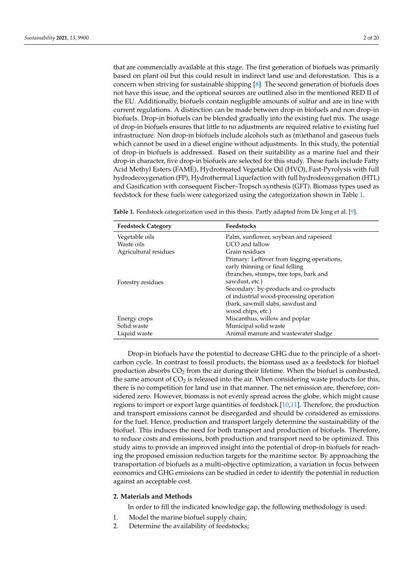
that are commercially available at this stage. The first generation of biofuels was primarilybased on plant oil but this could result in indirect land use and deforestation. This is aconcern when striving for sustainable shipping [8]. The second generation of biofuels doesnot have this issue, and the optional sources are outlined also in the mentioned RED II ofthe EU. Additionally, biofuels contain negligible amounts of sulfur and are in line withcurrent regulations. A distinction can be made between drop-in biofuels and non drop-inbiofuels. Drop-in biofuels can be blended gradually into the existing fuel mix. The usageof drop-in biofuels ensures that little to no adjustments are required relative to existing fuelinfrastructure. Non drop-in biofuels include alcohols such as (m)ethanol and gaseous fuelswhich cannot be used in a diesel engine without adjustments. In this study, the potentialof drop-in biofuels is addressed. Based on their suitability as a marine fuel and theirdrop-in character, five drop-in biofuels are selected for this study. These fuels include FattyAcid Methyl Esters (FAME), Hydrotreated Vegetable Oil (HVO), Fast-Pyrolysis with fullhydrodeoxygenation (FP), Hydrothermal Liquefaction with full hydrodeoxygenation (HTL)and Gasification with consequent Fischer–Tropsch synthesis (GFT). Biomass types used asfeedstock for these fuels were categorized using the categorization shown in Table 1.

Table 1. Feedstock categorization used in this thesis. Partly adapted from De Jong et al. [9].

Feedstock Category Feedstocks

Vegetable oils Palm, sunflower, soybean and rapeseedWaste oils UCO and tallowAgricultural residues Grain residues

Forestry residues

Primary: Leftover from logging operations,early thinning or final felling(branches, stumps, tree tops, bark andsawdust, etc.)Secondary: by-products and co-productsof industrial wood-processing operation(bark, sawmill slabs, sawdust andwood chips, etc.)

Energy crops Miscanthus, willow and poplarSolid waste Municipal solid wasteLiquid waste Animal manure and wastewater sludge

Drop-in biofuels have the potential to decrease GHG due to the principle of a short-carbon cycle. In contrast to fossil products, the biomass used as a feedstock for biofuelproduction absorbs CO2 from the air during their lifetime. When the biofuel is combusted,the same amount of CO2 is released into the air. When considering waste products for this,there is no competition for land use in that manner. The net emission are, therefore, con-sidered zero. However, biomass is not evenly spread across the globe, which might causeregions to import or export large quantities of feedstock [10,11]. Therefore, the productionand transport emissions cannot be disregarded and should be considered as emissionsfor the fuel. Hence, production and transport largely determine the sustainability of thebiofuel. This induces the need for both transport and production of biofuels. Therefore,to reduce costs and emissions, both production and transport need to be optimized. Thisstudy aims to provide an improved insight into the potential of drop-in biofuels for reach-ing the proposed emission reduction targets for the maritime sector. By approaching thetransportation of biofuels as a multi-objective optimization, a variation in focus betweeneconomics and GHG emissions can be studied in order to identify the potential in reductionagainst an acceptable cost.

2. Materials and Methods

In order to fill the indicated knowledge gap, the following methodology is used:

1. Model the marine biofuel supply chain;2. Determine the availability of feedstocks;

Sustainability 2021, 13, 9900 3 of 20

3. Determine the future demand for marine biofuel;4. Determine the required model parameters;5. Perform a scenario analysis.

Starting with the development of a multi-objective strategical supply chain optimiza-tion model, these steps are executed chronologically.

2.1. Mathematical Model Formulation

This section contains the mathematical formulation of the multi-objective MixedInteger Linear Programming (MILP) model. The corresponding nomenclature is provided.A schematic representation of the model is given in Figure 1. The world is divided into 18regions in which the main bunker hubs are used as nodes in the network. The followingsubsections contain the economic objective, environmental objective and model constraints.

Figure 1. Schematic representation of the modeled supply chain.

2.1.1. Economic Objective

The economic objective is to minimize total system costs. These total system costsare dependent on four decision variables. Three of these decision variables are related tothe flow inside the system and are continuous. The fourth is an integer variable whichindicates how many refineries of size p ∈ P and type g ∈ G are located at refinery noder ∈ R. The decision variable BFsbjit indicates the amount of biomass of type b ∈ B of supplyinterval i ∈ I that is processed into intermediate j ∈ J at supply node s ∈ S during timeperiod t ∈ T. The decision variable IFsrjt specifies the flow of intermediate product j ∈ Jthat is transported from supply node s ∈ S to refinery node r ∈ R during time period t ∈ T.The decision variable FFrdgt reveals the amount of biofuel type g ∈ G that flows betweenrefinery node r ∈ R and demand node d ∈ D during time period t ∈ T. The final decisionvariable, Yrgpt, indicates if a refinery of size p ∈ P producing fuel g ∈ G is operational atthe candidate location r ∈ R during time period t ∈ T.

These four decision variables, combined with several parameters, are used to formu-late the following economic objective function.

Objeco = Min. C (1)

Total costs can be separated into three parts: the costs of the intermediate product,the costs of upgrading the intermediate to a biofuel and the cost of sea transport.

C = ∑t∈T

(CIt + CU

t + CTt ) (2)

Costs of the intermediate product are dependent on the region and the feedstocksthat they are made from. It is assumed that a processing facility in a certain area onlyuses feedstocks that originate from that area. These costs can again be subdivided into

Sustainability 2021, 13, 9900 4 of 20

three parts. The costs related to the intermediate product consist of feedstock, processingand inland transport costs.

CIt = CIB

t + CIPt + CIT

t (3)

The feedstock costs are the costs of the different types of biomass b ∈ B at locations ∈ S during time period t ∈ T.

CIBt = ∑

s∈S∑b∈B

∑j∈J

ubcsb · BFsbjit ∀t ∈ T (4)

The processing costs are expressed as the costs related to producing intermediateproduct j ∈ J from biomass type b ∈ B at supply location s ∈ S. An assumption ismade that the processing costs are only dependent on the area in which the processingis performed. Spatial optimization of the processing facilities is outside the scope of thisthesis. The reason for this is the assumption that long-distance transport of low-densitybiomass would not be efficient. Therefore, smaller distributed processing facilities wouldalways be located near the harvest site.

CIP = ∑s∈S

∑b∈B

∑j∈J

upcsj · IFsrjt ∀t ∈ T (5)

The third part of CIt includes the inland transport of the biomass to the processing

facility. Generally, the supply costs of biomass are depicted as cost/supply curves. Re-gional biomass costs rise when the required supply increases. Initially, biomass that isnearest to the processing facility and most easy to gather is used. When demand increases,biomass that is more difficult to access and is further from the processing facility will beused, increasing transport distance and costs consequently. In order to mimic this, inlandtransport costs are expressed as a linear function of the biomass flow inside the supplyareas. However, this property induces a non-linear relationship between the biomass flowand inland transport costs. Therefore, the function is cut up into five discrete cost segmentsfor every biomass type and region combination.

Using the above described method, the total inland transport costs of biomass forevery t ∈ T can be calculated using the following expression. Observing that biomass isusually of low density, the volume is assumed to be the limiting factor.

CITt = ∑

s∈S∑b∈B

∑j∈J

(uitcs · ρb ·BFsbjit

lhvbb) ∀t ∈ T (6)

The second cost item includes the costs that are related to setting up and operating anupgrading facility. These costs can be divided into variable and fixed costs.

CUt = CUV

t + CUFt ∀t ∈ T (7)

In the optimization model of Lin et al. [12], the Operational Expenses (OPEXs) wereconsidered to be independent of the refinery capacity. In this model, the same assumptionis made. However, OPEXs are dependent on the location in which the refinery operates.The OPEXs are calculated separately from the feedstock costs, which were already includedin CIB

t .In general, part of the OPEX can be seen as variable costs and another part as fixed

costs. CUV only includes the variable part of the OPEX, which is dependent on the producedamount of biofuel.

CUVt = ∑

r∈R∑

g∈G∑

d∈Duvcrgt · FFrdgt ∀t ∈ T (8)

In Equation (8), uvcrgt represents the OPEX per energy output of biofuel g ∈ G atlocation r ∈ R during time period t ∈ T. The Capital Expenses (CAPEXs) are annualized

Sustainability 2021, 13, 9900 5 of 20

over the lifetime and are added to the fixed part of the refinery OPEX. This is expressed inEquation (9).

CUFt = ∑

r∈R∑

g∈G∑p∈P

u f crgpt ·Yrgpt ∀t ∈ T (9)

The decision variable Yrgpt is an integer that indicates if a plant of size p ∈ P producingfuel g ∈ G at location r ∈ R is operational during time period t ∈ T.

Lastly, transport costs are divided into the costs for the transportation of the interme-diate products and the end products.

CTt = CIT

t + CFTt ∀t ∈ T (10)

CITt = ∑

s∈S∑r∈R

∑j∈J

(ustcsr ·IFsrjt

lhvjj) ∀t ∈ T (11)

CFTt = ∑

r∈R∑

d∈D∑

g∈G(ustcrd ·

FFrdgt

lhvgg) ∀t ∈ T (12)

2.1.2. Environmental Objective

The environmental objective is to minimize the total GHG emissions related to thesupply of marine biofuels. The same decision variables as introduced in the previoussection are used for the environmental optimization. In order to determine the GHGemissions of the marine biofuel supply chain, the method of Giarola et al. [13] is used as astarting point. The life-cycle emissions are separated into different phases. The objective isto minimize total system emissions, as expressed in Equation (13).

Objenv = Min. E (13)

These total system emissions can be divided into emissions related to the intermediatebio-energy carrier, upgrading the intermediate to a biofuel and transport, which can beevaluated as follows.

E = ∑t∈T

(EIt + EU

t + ETt ) (14)

Firstly, an expression that represents the emissions caused by the production ofthe intermediate bio-energy carrier is developed. These emissions can be split up intoemissions caused by harvesting, gathering and processing of the feedstocks. Moreover,inland transport of the feedstock needs to be considered.

EIt = EIB

t + EIPt + EIT

t ∀t ∈ T (15)

Emissions caused by harvesting and gathering of the feedstocks are assumed to beproportional to the flow of biomass inside the supply regions.

EIBt = ∑

s∈S∑b∈B

∑j∈J

BFsbjt · e fsb ∀t ∈ T (16)

Furthermore, the feedstock will be processed into an intermediate energy carrier.The emissions related to this conversion are proportional to the amount of intermedi-ate produced.

EIPt = ∑

s∈S∑r∈R

∑j∈J

IFsrjt · epsj ∀t ∈ T (17)

The inland transport costs are considered as a constant for every region and biomasstype. An average distance is assumed dependent on the size of the region. Furthermore,

Sustainability 2021, 13, 9900 6 of 20

the same approach as explained in Section 2.1.1 is used to simulate increasing inlandtransport emissions due to increasing distance when more supply is needed.

EITt = ∑

s∈S∑b∈B

∑j∈J

BFsbjt ·eitsblhvbb

∀t ∈ T (18)

For the emissions related to the upgrading of the intermediate bio-energy carrier tothe eventual biofuel, the following expression is used.

EUt = ∑

r∈R∑

d∈D∑

g∈GFFrdgt · eug ∀t ∈ T (19)

Additionally, there are emissions associated with the overseas transport of both theintermediate bio-energy carrier and the biofuel.

ETt = ETI

t + ETFt (20)

These emissions are caused by the combustion of fossil products of the tankers whichtransport the goods. Both the flow of the intermediate products and the biofuel productsare multiplied with an emission factor that is dependent on the distance between the nodes.

ETIt = ∑

s∈S∑r∈R

∑j∈J

IFsrjt · estsr ∀t ∈ T (21)

ETFt = ∑

r∈R∑

d∈D∑

g∈GFFrdgt · estrd ∀t ∈ T (22)

2.1.3. Constraints

Firstly, all four decision variables are not allowed to take on negative values.

BFsbjit ≥ 0 ∀s ∈ S, b ∈ B, j ∈ J, i ∈ I, t ∈ T (23)

IFsrjt ≥ 0 ∀s ∈ S, r ∈ R, j ∈ J, t ∈ T (24)

FFrdgt ≥ 0 ∀r ∈ r, d ∈ D, g ∈ G, t ∈ T (25)

Yrgpt ≥ 0 ∀r ∈ R, g ∈ G, p ∈ P, t ∈ T (26)

Secondly, flow equilibrium constraints are required to ensure that the flow of goodsstays consistent throughout the solution. Equation (27) ensures equilibrium in every supplynode between biomass flow in and intermediate flow out.

∑b∈B

(BFsbjit ·ωbj)− ∑r∈R

IFsrjt = 0 ∀s ∈ S, t ∈ T, j ∈ J (27)

Equation (28) is established to ensure equilibrium in all refinery nodes.

∑s∈S

∑j∈J

(IFsrjt · γjg)− ∑d∈D

FFrdgt = 0 ∀r ∈ R, g ∈ G, t ∈ T (28)

An additional constraint is used to prevent flow from going through nodes where norefinery is built. For this purpose, the big-M method is used. M represents a new parameterto which a large number is assigned. Hence, a yes or no decision can be formulatedas follows.

∑p∈P

Yrgpt ·M ≥ ∑d∈D

FFrdgt ∀g ∈ G, r ∈ R, t ∈ T (29)

Sustainability 2021, 13, 9900 7 of 20

In order to ensure that the global biomass availability is not exceeded, a constraintis required per region that limits the amount of biomass used by all ports in that region.For every distinct region in H a separate constraint is composed, shown in Equation (30).

∑j∈J

BFsbjt ≤ f caphbt ∀h ∈ H, s ∈ S, t ∈ T, b ∈ B (30)

Additionally, the refinery capacity at a refinery node r ∈ R may not be exceeded.Moreover, only intermediate flow can go through refinery node r ∈ R if a plant opened atthat location. When there is no capacity at a refinery node r ∈ R, the right-hand side ofEquation (31) becomes zero, forcing the intermediate flow through that node to be zero.

∑s∈S

∑j∈J

(IFsrjt · γjg) ≤ ∑p∈P

(rcappg ·Yrgpt) ∀r ∈ R, g ∈ G, t ∈ T (31)

Equation (32) of this minimum cost flow-facility location problem is that the sumof the fuel flows to the demanded nodes equal the demand in that specific node. Thisconstraint can be written as follows.

∑r∈R

∑g∈G

FFrdgt = d fdt ∀d ∈ D, t ∈ T (32)

Additionally, to render the linearization of the inland transports costs possible, as dis-cussed in Section 2.1.1, limits for the amount of biomass taken from a particular supplystep need to be set up. Therefore, two extra parameters need to be included in the model,λlow

sbi and λhighsbi , indicating the lower and upper limits of the supply steps. Consequently,

the following constraints are set up to ensure the correct price is paid for the amount ofsupply used.

∑j∈J

BFsbjit ≥ λlowsbi ∀s ∈ S, b ∈ B, i ∈ I, t ∈ T (33)

∑j∈J

BFsbjit ≤ λhighsbi ∀s ∈ S, b ∈ B, i ∈ I, t ∈ T (34)

Constraints are required to ensure that when a refinery is built, it stays active for agiven period of time. In the model, it is assumed that only one refinery of type g ∈ G canbe operational at every refinery node r ∈ R during t ∈ T. However, the scale of the refinerymay vary. This constraint is optional; if it turns out that more refineries per location areneeded in order to fulfill the demand, then this constraint will be dropped.

∑p∈P

Yrgpt ≤ 1 ∀r ∈ R, g ∈ G, t ∈ T (35)

Equation (36) ensures that if a refinery is built during time period t ∈ T, it can onlygrow to a bigger facility in the next time period, or it stays the same size. This allows forthe possibility to expand a refinery over time.

∑p∈P

(Yrgpt−1 · rcappg) ≤ ∑p∈P

(Yrgpt · rcappg) ∀r ∈ R, g ∈ G, t ∈ T (36)

In order to add some additional features to the model, some optional constraints canbe implemented. The following constraint can be used to prohibit a conversion technologyto be used in a certain time period. Some conversion pathways might become mature inthe far future, while others may be used from the start. In this case, t∗ is the time period inwhich the conversion technology g∗ is not available.

∑r∈R

∑d∈D

FFrdg∗t∗ = 0 (37)

Sustainability 2021, 13, 9900 8 of 20

Additionally, some fuels might be subjected to a blend wall. This could be imple-mented by using a constraint that prohibits exceeding this blend wall. If a blend limit isimposed on fuel g∗ and the blend limit is expressed as blendlim, than that constraint wouldlook as follows.

∑r∈R

FFrdg∗t ≤ blendlim ∀d ∈ D, t ∈ T (38)

Lastly, it is assumed that if a product is gaseous then it cannot be transported. In thiscase, the amount of biomass used for the production of intermediate j∗ in a certain nodeshould be equal to the amount of intermediate j∗ used for the production of biofuel inthat node.

∑i∈I

∑b∈B

BFsbj∗it = IFssj∗t ∀s ∈ S, t ∈ T (39)

2.2. Supply and Demand Scenarios

For the strategical supply chain optimization, several supply and demand scenarioswere developed (see Table 2 for an overview). Taken together, a total of eighteen distinctscenarios were simulated. A more detailed elaboration on these scenarios is given in thefollowing two sections.

Table 2. Description of supply and demand scenarios settings used in this study.

Geographical Scenario Settings Supply Scenario Settings Demand Scenario Settings

Europe Low Supply (LS) Low Demand (LD)European ports comply with the RED IItarget of 14 % renewable fuel in theirtransport mix by 2030, reflecting asituation in which shipping is included inthis target. Double counting mechanismsare not considered. A linear trend isassumed, reaching up until 2050.

The LS scenario contains a conservativeestimation on biomass feedstockavailability combined with significantcompetition from other industries.

The LD scenario uses scenario 11 of theThird GHG Study of the IMO [14].

Most Likely (ML) High Supply (HS) Base Demand (BD)

Leading countries in sustainability (theUSA, The Netherlands, Germany, Canadaand the UK) are assumed to follow theRED II targets.

The HS scenario contains a moreoptimistic view on biomass feedstockavailability that would be available forthe production of marine biofuels.The road sector is expected to electrify ata fast pace, causing lower competition forcertain biomass feedstocks.

The BD scenario uses scenario 8 of theThird GHG Study of the IMO [14].

World High Demand (HD)All ports are assumed to achieve the IMOtarget of 50% GHG reduction by 2050compared to 2008 levels.

The HD scenario uses scenario 14 of theThird GHG Study of the IMO [14].

2.2.1. Biomass Supply Scenarios

In a study by De Jong et al. [9], the amount of available biomass in the EU to supplythe aviation sector was analyzed. He indicated that there is uncertainty embedded in thedetermination of domestic availability and import potential of biomass. To capture thisuncertainty, De Jong et al. [9] developed several supply and demand scenario. Although ona broader spatial scale, this study uses a similar approach. Low Supply (LS) and HighSupply (HS) scenarios are developed based on feedstock availability and competing in-dustries. In the LS scenario, a conservative estimation of biomass availability is combinedwith high competition from other industries. In the HS scenario a more optimistic viewon biomass availability is combined with less competition from other industries. In orderto determine the amount of biomass available for the production of marine biofuels, firstly,the domestic availability of each feedstock category in each region is estimated by means of

Sustainability 2021, 13, 9900 9 of 20

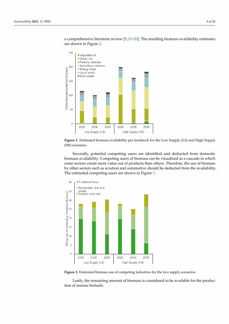
a comprehensive literature review [9,15–20]. The resulting biomass availability estimatesare shown in Figure 2.

Figure 2. Estimated biomass availability per feedstock for the Low Supply (LS) and High Supply(HS) scenarios.

Secondly, potential competing users are identified and deducted from domesticbiomass availability. Competing users of biomass can be visualized as a cascade in whichsome sectors create more value out of products than others. Therefore, the use of biomassby other sectors such as aviation and automotive should be deducted from the availability.The estimated competing users are shown in Figure 3.

Figure 3. Estimated biomass use of competing industries for the two supply scenarios.

Lastly, the remaining amount of biomass is considered to be available for the produc-tion of marine biofuels.

Sustainability 2021, 13, 9900 10 of 20

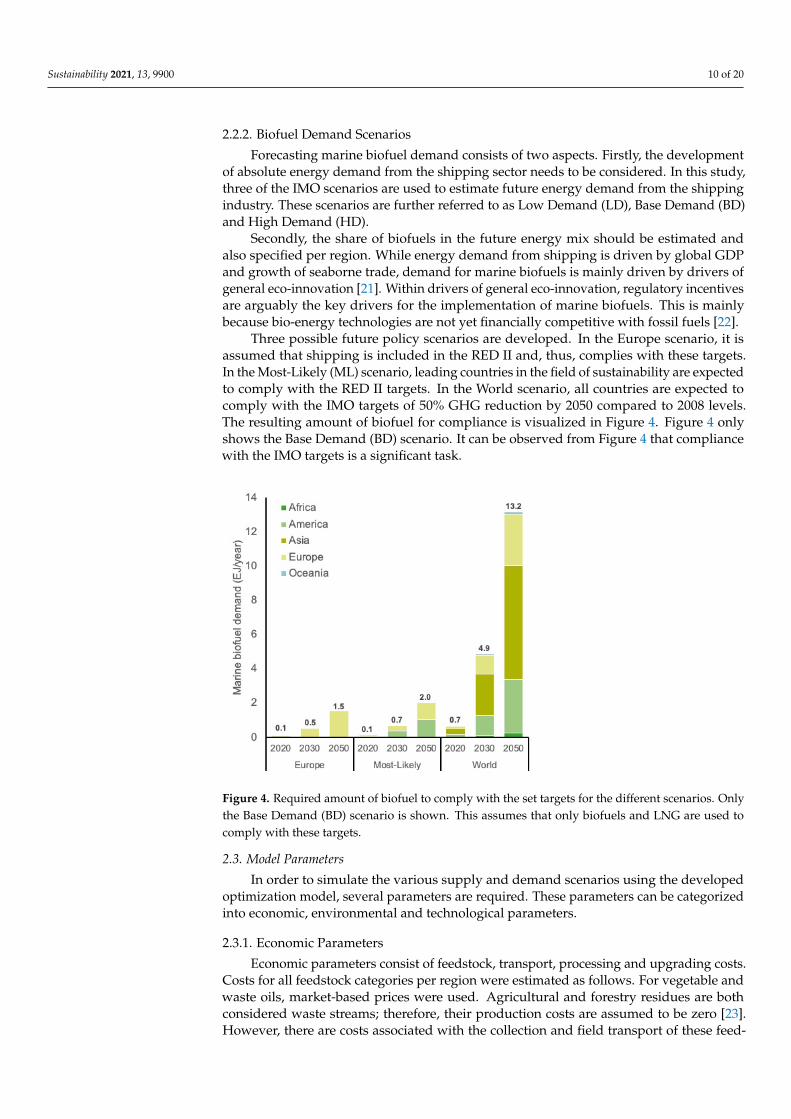
2.2.2. Biofuel Demand Scenarios

Forecasting marine biofuel demand consists of two aspects. Firstly, the developmentof absolute energy demand from the shipping sector needs to be considered. In this study,three of the IMO scenarios are used to estimate future energy demand from the shippingindustry. These scenarios are further referred to as Low Demand (LD), Base Demand (BD)and High Demand (HD).

Secondly, the share of biofuels in the future energy mix should be estimated andalso specified per region. While energy demand from shipping is driven by global GDPand growth of seaborne trade, demand for marine biofuels is mainly driven by drivers ofgeneral eco-innovation [21]. Within drivers of general eco-innovation, regulatory incentivesare arguably the key drivers for the implementation of marine biofuels. This is mainlybecause bio-energy technologies are not yet financially competitive with fossil fuels [22].

Three possible future policy scenarios are developed. In the Europe scenario, it isassumed that shipping is included in the RED II and, thus, complies with these targets.In the Most-Likely (ML) scenario, leading countries in the field of sustainability are expectedto comply with the RED II targets. In the World scenario, all countries are expected tocomply with the IMO targets of 50% GHG reduction by 2050 compared to 2008 levels.The resulting amount of biofuel for compliance is visualized in Figure 4. Figure 4 onlyshows the Base Demand (BD) scenario. It can be observed from Figure 4 that compliancewith the IMO targets is a significant task.

Figure 4. Required amount of biofuel to comply with the set targets for the different scenarios. Onlythe Base Demand (BD) scenario is shown. This assumes that only biofuels and LNG are used tocomply with these targets.

2.3. Model Parameters

In order to simulate the various supply and demand scenarios using the developedoptimization model, several parameters are required. These parameters can be categorizedinto economic, environmental and technological parameters.

2.3.1. Economic Parameters

Economic parameters consist of feedstock, transport, processing and upgrading costs.Costs for all feedstock categories per region were estimated as follows. For vegetable andwaste oils, market-based prices were used. Agricultural and forestry residues are bothconsidered waste streams; therefore, their production costs are assumed to be zero [23].However, there are costs associated with the collection and field transport of these feed-

Sustainability 2021, 13, 9900 11 of 20

stocks [24]. For Europe, values from Hoogwijk and Graus [20], De Wit and Faaij [24], Allenet al. [25] and Ericsson et al. [26] are used. Since the costs for both agricultural and forestryresidues are dominated by collection and field transport, the costs in Europe are scaledwith a combination of regional labor costs and gasoline prices to obtain values for allother regions.

For lignocellulosic energy crops, costs of perennial grasses from Ericsson et al. [26]are used for Europe. De Wit and Faaij [24] stated that factors that dominate the costs ofenergy crops are land costs, wage level and production efficiency. Therefore, the base costsof energy crops are scaled with regional labor costs and gasoline prices. Liquid wastesand solid wastes are considered as residue streams. In contrast to agricultural and forestryresidues, these waste types can be collected in centralized waste collection plants. Thiscauses gathering and transport costs to be zero.

Hoogwijk and Graus [20] estimated costs of residues and energy crops for all worldregions. However, they found residue prices to be uncertain. As an example, they indicatedresidue prices in OECD Europe to be between 0.9 and 10.5 EUR/GJ, which is an extremelylarge range. Alves et al. [27] states that “Biomass feedstock cost plays a major impact inthe operational costs of a plant and the uncertainty associated with the feedstock supplyis the most critical aspect of bio-refineries profitability”. Hence, feedstock costs havea significant contribution to refinery operating costs but are simultaneously uncertain.Therefore, feedstock costs should be further studied in the sensitivity analysis. Since atwo-stage supply chain is considered, costs for processing and upgrading are separatedand visualized in Figure 5.

Figure 5. Processing and upgrading costs for different technologies. Data from [9,28–40,40–46].

2.3.2. Environmental Parameters

Analogous to the economic parameters, emission factors can be assigned to differentlife-cycle phases of the end product. To determine the allocation of GHG emissions to thelife-cycle of the fuel, the method of the RED II is used. For the cultivation of feedstocks,default values from the RED II were used. Emission factors related to processing andupgrading of the fuel were obtained from the RED II and a Life-Cycle Analysis (LCA) ofDe Jong et al. [47].

Unit emissions for transport were taken from McKinnon and Piecyk [48]. Unit emis-sions from sea transport are highly dependent on the vessel type, trade route, and corre-sponding vessel utilization rate. For short-sea and deep-sea shipping, average emissionfactors of 16 and 12 gCO2-eq/ton-km are used, respectively [48].

Sustainability 2021, 13, 9900 12 of 20

2.3.3. Technological Parameters

Process yields are defined as the amount of biofuel that can be produced from a certainquantity of biomass. In this case, two conversion yields are of importance: the yield frombiomass to the bio-intermediate and the yield from the bio-intermediate to the biofuel endproduct. Conversion yields are dependent on the process conditions and the molecularcomposition of feedstocks. For example, grain residues have a high ash content which canreduce its conversion yield [30]. Examples of process conditions that can affect the yieldsare temperature, solvent-to-feedstock ratio (for fast pyrolysis) and the fluidizing medium(for GFT) [30]. In order to obtain a realistic estimation of these process yields, an average istaken from the values of different literature sources. The resulting values are visualized inFigure 6.

Figure 6. Conversion yields for different technologies. Data from [28–34,37–39,41–46,46,49–53].

3. Results

In this section, the results from simulating the proposed supply and demand scenariousing the developed MILP model are displayed. Results can be subdivided into threecategories. Firstly, cost and emission projections associated with the large scale use ofmarine biofuels are depicted. This also includes the marginal costs of GHG reduction.Secondly, the most feasible deployment of various feedstock and conversion technologycombinations is shown. Lastly, the most feasible trade flows of the intermediate bio-energycarriers and biofuels are elaborated upon. These results give an impression of the expectedexport and import regions of biomass and biofuel.

3.1. Costs Versus Emissions

The multi-objective optimization induces a trade-off between costs and emissions.The resulting marginal costs of GHG reduction for all scenarios are visualized in Figure 7.In every run, this trade-off is reconsidered to reach the highest GHG reduction against thelowest costs. A clear trade-off between costs and emission reduction is visualized. The mostbeneficial trade-off is found to be around 80% GHG reduction compared to Heavy Fuel Oil(HFO), which corresponds to the average fuel costs of around 900–1050 EUR/ton of biofuel.

In Figure 8, the average fuel costs per time period are displayed. These costs areobtained by dividing the total expenses of that time period by the amount of fuel producedduring that time period. It should be noted that these are average costs; in reality, differentcosts would be allocated to different fuel types. It stands out that, at first, fuel costs declineas a result of scale advantages and the use of cheaper feedstocks. However, after a strong

Sustainability 2021, 13, 9900 13 of 20

decrease, costs gradually go up again. Rising demand induces the need for feedstocks thatare increasingly difficult to collect, driving up the feedstock costs.

Figure 7. Marginal costs of Green House Gas reduction compared to HFO. A Well-to-Wake emissionfactor of 87.5 gCO2-eq/MJ for HFO was used.

Figure 8. Projected average biofuel costs over the studied time period.

The results showed that around 20% of the costs are related to the raw materials, and50% of the costs are associated with the production of the intermediate bio-energy carrier.The remaining 30% is related to the upgrading process. On the contrary, the upgradingprocess is responsible for around 85% of total GHG emissions. This is a result of thegenerous amounts of hydrogen required for the upgrading process. It is assumed thatthe used hydrogen originates from fossil sources. Using hydrogen from the of-gasses ofthe process or sourcing green hydrogen would make an enormous impact on the GHGreduction potential of drop-in biofuels. Additionally, it could be argued if drop-in biofuelsfor marine purposes require vast amounts of upgrading. Marine engines are often built forheavy-duty operations and residual or low quality fuel.

Sustainability 2021, 13, 9900 14 of 20

3.2. Technology and Feedstock Deployment

A total of five drop-in biofuel production pathways were considered in this study.In the first time period, only FAME and HVO were considered to be commercially available.After 2025, Fast-Pyrolysis (FP) and Gasification Fischer–Tropsch (GFT) were introduced.Hydrothermal Liquefaction (HTL) was introduced after 2030.

In all studied scenarios, HTL showed to be the most promising fuel both on economicand environmental performance. The main causes for this are the minor amount of up-grading required compared to Fast-Pyrolysis and the possibility in using a wide varietyof feedstocks, including manure and sludges. However, the potential of HTL could beinhibited by its low TRL (Technology Readiness Level).

Feedstock deployment resulted in a mix of feedstocks, with a small preference forthe use of agricultural residues. The reason for this mix can be partly attributed to theexisting trade-off between costs, environmental performance and technological efforts [54].As an example, waste streams such as manure and Municipal Solid Waste (MSW) arecheap and have a high emission reduction potential. However, it is extremely difficult toobtain a constant stream that is suitable for the production of biofuel with steady quality.For residues from agricultural and forestry practices, feedstock costs rise when demandincreases due to the need for feedstocks that become increasingly difficult to collect.

In Figure 9, the enormous refinery capacities required to reach the proposed targets arelined up for the three geographical demand scenarios. To place this in perspective, commonbiorefinery sizes mentioned in the literature are in the range of 1000–2000 dry ton input per day.This would correspond to an estimated biorefinery output of 0.0035–0.007 EJ/yr (usingan average feedstock energy density of 18 MJ/kg and conversion yield of 0.6). In orderto comply with the GHG reduction target of the IMO by 2050, this would impose a requiredinvestment in the range of 1100–2200 new biorefineries of that size worldwide during thestudied time period. This provides an idea of the enormous challenges that lie ahead.

Figure 9. Required bio-refinery capacity per region to comply with the targets proposed in thedeveloped scenarios. Capacity is given in the required refinery output. Integers represent the studiedtime intervals. 1: 2020–2025; 2: 2025–2030; 3: 2030–2035; 4: 2035–2040; 5: 2040–2045; 6: 2045–2050.

3.3. Trade Flows

Lastly, after the determination of the spatial distributions of future marine biofueldemand and feedstock availability, imbalances in supply and demand are found. Espe-cially in the first time period, when oils and fats are the only usable feedstocks, significantimbalances exist. This is confirmed by a large amount of trade in vegetable and waste

Sustainability 2021, 13, 9900 15 of 20

oils. The MILP model developed in this study assumes that biomass is converted to anintermediate bio-energy carrier before it is transported between regions. Hence, a distinc-tion can be made between the trade of the intermediate bio-energy carrier and trade of thebiofuel end-product.

Figure 10 displays the most feasible exports and imports of the intermediate productbetween regions. The exporting regions can also be identified as the biomass exportingregions, seeing that the processing step is always performed in the domestic region. In theEurope scenario, a large difference between the LS and HS scenarios exist. This is mainlycaused by the increased availability of oils and fats in the HS scenario. This causes NorthernAmerica to gain more export opportunities, which is mainly caused by less competitionfrom the road and aviation sector for these feedstocks in this scenario.

In the Most-Likely scenario, Eastern Asia and Southern Asia are the major suppliersof the intermediate product. In the World scenario, Southern Asia is the dominant exporter,which is mainly caused by the large availability of animal manure in that region. Despitethe large technological efforts associated with the conversion of this feedstock, the modelchooses to use this feedstock for the production of biofuels.

Figure 10. Intermediate bio-energy carrier exports and imports per region for all studied scenariosduring the entire time period.

On the other side, intermediate imports are more centralized. These importing regionsare relatively constant and are highly dependent on the spatial distribution of fuel demand.In the European scenario, Western Europe and Southern Europe are expected to importintermediate products. In the ML scenarios, Northern America is included in this group.In the World scenario, a shift in demand causes Asian regions to become the main importers.

Exports and imports of biofuels are displayed in Figure 11. From this figure, it canbe observed that biofuel exports are dominated by Southern Europe in the Europe andML scenario. Hence, Southern Europe is considered the most preferable spot to constructbiorefineries. This is mainly caused by its central location and beneficial local operatingcosts. Elements such as available infrastructure and local subsidies for attracting this typeof business have not been taken into account.

Figure 11 shows that importing regions of biofuel are more diverse. In these importingregions, a shortage on refinery capacity results in the need for imports. In the Europeanscenario, most biofuels are imported to Western and Northern Europe. In the ML scenario,Northern America also imports a fair share of biofuel. The importing regions of biofuel inthe World scenario are somewhat more distributed. The large share of South Eastern Asia

Sustainability 2021, 13, 9900 16 of 20

can be dedicated to the presence of Singapore in that area, which on its own is responsiblefor around 20% of global fuel sales.

Figure 11. Biofuel exports and imports per region for all studied scenarios during the entire time period.

4. Conclusions

In this study, the potential of drop-in biofuels for the maritime industry was assessed.In order to measure this potential, a strategic supply chain optimization was performed todetermine the economic and environmental performance of drop-in biofuels. Additionally,a comprehensive scenario analysis identified the availability of biomass and the requiredinvestments in new infrastructure and technologies to achieve the proposed GHG reductiontargets of the RED II and IMO.

Concerning the economic performance of drop-in biofuels, the price gap with fos-sil products is still large. Although technological learning effects were not considered,the production costs of drop-in biofuel were projected to initially decrease. This is mainlycaused by the gradually growing influence of economies of scale in combination with theintroduction of new technologies that are able to use cheaper feedstocks. However, drop-inbiofuels could also be the victim of their own success. In contrast to other renewable fuels,increasing demand results in the need for more expensive feedstocks that are difficultto collect.

The possible GHG reduction potential of drop-in biofuels was found to be between 68and 95% compared to HFO for a cost of 850–2300 EUR/ton. Emission reductions of 80%compared to HFO are estimated to be achieved at fuel costs of around 900–1050 EUR/ton.

The availability of oils and fats is a severe barrier to the scalability of drop-in biofuels.Additionally, it could be argued if dependency on waste oils for the production of marinefuels is desirable. This increases the urgency for the rapid development of new conversiontechnologies that pave the road for the usage of more abundant feedstocks. It has beenshown that in order to achieve the proposed emission reduction targets, enormous invest-ments in new biorefineries are required. This entails investments in smaller processingfacilities located near the feedstock source and larger refinery hubs located near ports.

In conclusion, drop-in biofuels offer a significant GHG reduction potential for theshipping industry. These fuels can be used without adaptations to existing fuel infrastruc-ture. FAME and HVO are already commercially available, but limited feedstock availabilityinduces the need for investments in new conversion technologies. When these technologiesbecome available, enough biomass is domestically available to serve a large part of theshipping industry.

Sustainability 2021, 13, 9900 17 of 20

Author Contributions: Conceptualization, J.F.J.P. and D.F.A.v.d.K.; methodology, D.F.A.v.d.K.; soft-ware, D.F.A.v.d.K.; validation, D.F.A.v.d.K. and J.F.J.P.; formal analysis, D.F.A.v.d.K.; investigation,D.F.A.v.d.K.; resources, D.F.A.v.d.K.; data curation, D.F.A.v.d.K.; writing—original draft preparation,D.F.A.v.d.K.; writing—review and editing, J.F.J.P.; visualization, D.F.A.v.d.K.; supervision, J.F.J.P.;project administration, J.F.J.P.; funding acquisition, J.F.J.P. All authors have read and agreed to thepublished version of the manuscript.

Funding: This research was funded by NML grant number IC B18022020 RH 0014. The study wasfurther supported by (in kind) contributions of MKC and Goodfuels. The APC was funded by acentral agreement of TU Delft with MDPI.

Institutional Review Board Statement: Not applicable.

Informed Consent Statement: Not applicable.

Data Availability Statement: Not applicable.

Conflicts of Interest: The authors declare no conflict of interest. The funders had no role in the designof the study; in the collection, analyses, or interpretation of data; in the writing of the manuscript, orin the decision to publish the results.

Nomenclature

S Set of supply nodes.R Set of candidate refinery nodes.D Set of demand nodes.H Set of regions.B Set of biomass feedstocks.J Set of intermediate products.G Set of end products.P Set of plant sizes.I Set of supply steps.T Set of time periods.

BFsbjitUsed amount of biomass b ∈ B of supply step i ∈ I at supply node s ∈ Sto produce intermediate product j ∈ J during time period t ∈ T (PJ).

IFsrjtFlow of intermediate j ∈ J between supply node s ∈ S and refinerynode r ∈ R during time period t ∈ T (PJ).

FFrdgtFlow of biofuel g ∈ G between refinery node r ∈ R and demand noded ∈ D during time period t ∈ T (PJ).

YrgptVariable that indicates if a refinery of size p ∈ P producing biofuelg ∈ G at refinery node r ∈ R is built during time period t ∈ T.

ubcsbtUnit costs of biomass b ∈ B at supply node s ∈ S during time periodt ∈ T (mln €/PJ).

upcsbjtUnit costs of producing intermediate j ∈ J from biomass b ∈ B at supplynode s ∈ S during time period t ∈ T (mln €/PJ).

uitcsbtUnit costs for inland transport of biomass b ∈ B to supply node s ∈ Sduring time period t ∈ T (mln €/kton).

uvcrgtVariable costs related to running a refinery producing biofuel g ∈ G atrefinery node r ∈ R during time period t ∈ T (mln €/PJ).

u f crgptAnnualized fixed costs of running a refinery of size p ∈ P producingfuel g ∈ G at refinery node r ∈ R in time period t ∈ T (mln €/5 years).

Sustainability 2021, 13, 9900 18 of 20

ustcsrUnit overseas transport costs between supply node s ∈ S and refinerynode r ∈ R (mln €/kton).

e fb Emissions related to cultivation of feedstock b ∈ B (kton CO2-eq/PJ).

epjEmissions related to the conversion of biomass b ∈ B to intermediatej ∈ J (kton CO2-eq/PJ).

eitsiEmissions related to the inland transport at supply node s ∈ S in supplystep i ∈ I (kton CO2-eq/kton).

eug Emissions related to the upgrading to biofuel g ∈ G (kton CO2-eq/PJ).

estsrEmissions related to the sea transport in between nodes (ktonCO2-eq/kton).

lhvbb Lower heating value of biomass type b ∈ B (MJ/kg).lhvjj Lower heating value of intermediate product j ∈ J (MJ/kg).lhvgg Lower heating value of biofuel g ∈ G (MJ/kg).

d fdtBiofuel demand at demand location d ∈ D during time period t ∈ T(PJ).

rcappg Capacity of a refinery of size p ∈ P producing fuel g ∈ G (PJ).

f capsbtAvailability of feedstock b ∈ B at supply node s ∈ S during time periodt ∈ T (PJ).

γjg Conversion yield from intermediate product j ∈ J to biofuel g ∈ G.ωbj Conversion yield from biomass b ∈ B to intermediate j ∈ J.

λlowsbi

Lower boundary for biomass type b ∈ B in supply step i ∈ I at supplynode s ∈ S.

λhighsbi

Upper boundary for biomass type b ∈ B in supply step i ∈ I at supplynode s ∈ S.

ρbRatio between density of biomass type b ∈ B and the maximum freightdensity.

C Total system costs over the entire studied period.CI

t Costs related to the intermediate bio-energy carrier during t ∈ T.CIB

t Cost of biomass during t ∈ T.

CIPt

Costs of processing the intermediate bio-energy carrier to a biofuelt ∈ T.

CITt

Costs related to the inland transport of the intermediate bio-energycarrier during t ∈ T.

CUt Costs related to the upgrading process during t ∈ T.

CUVt Variable costs related to the upgrading process during t ∈ T.

CUFt Fixed costs related to the upgrading process during t ∈ T.

CTt Costs related to sea transport during t ∈ T.

CITt Costs related to sea transport of the intermediate product during t ∈ T.

CFTt Costs related to sea transport of the biofuel during t ∈ T.

E Total system emissions over the entire studied period.EI

t Emissions related to the intermediate product during t ∈ T.EIB

t Emissions related to cultivation and harvesting of biomass during t ∈ T.EIP

t Emissions related to the processing phase during t ∈ T.EIT

t Emissions related to the inland transport of biomass during t ∈ T.EU

t Emissions related to the upgrading phase during t ∈ T.ET

t Emissions related to sea transport during t ∈ T.

ETIt

Emissions related to the sea transport of the intermediate productsduring t ∈ T.

ETIt

Emissions related to the sea transport of the biofuel products duringt ∈ T.

Sustainability 2021, 13, 9900 19 of 20

References1. Tyrovola, T.; Dodos, G.; Kalligeros, S.; Zannikos, F. The introduction of biofuels in marine sector. J. Environ. Sci. Eng. A 2017,

6, 415–421. [CrossRef]2. EU. Reducing Emissions from the Shipping Sector. Available online: https://ec.europa.eu/clima/policies/transport/shipping_en

(accessed on 11 March 2021).3. McGill, R.; Remley, W.; Winther, K. Alternative Fuels for Marine Applications; A Report from the IEA Advanced Motor Fuels

Implementing Agreement; Publications Office of the European Union: Luxembourg, 2013; Volume 54.4. Moirangthem, K.; Baxter, D. Alternative Fuels for Marine and Inland Waterways; European Commission: Brussels, Belgium, 2016.5. Czermanski, E.; Cirella, G.; Oniszczuk-Jastrzabek, A.; Pawlowska, B.; Notteboom, T. An Energy Consumption Approach to

Estimate Air Emission Reductions in Container Shipping. Energies 2021, 14, 278. [CrossRef]6. Van Vliet, O.P.; Faaij, A.P.; Turkenburg, W.C. Fischer–Tropsch diesel production in a well-to-wheel perspective: A carbon, energy

flow and cost analysis. Energy Convers. Manag. 2009, 50, 855–876. [CrossRef]7. Bouman, E.A.; Lindstad, E.; Rialland, A.I.; Strømman, A.H. State-of-the-art technologies, measures, and potential for reducing

GHG emissions from shipping—A review. Transp. Res. Part D Transp. Environ. 2017, 52, 408–421. [CrossRef]8. Sustainable Shipping Initiative. The Role of Sustainable Biofuels in the Decarbonisation of Shipping; Technical Report; Sustainable

Shipping Initiative, SSI: London, UK, 2019.9. De Jong, S.; van Stralen, J.; Londo, M.; Hoefnagels, R.; Faaij, A.; Junginger, M. Renewable jet fuel supply scenarios in the European

Union in 2021–2030 in the context of proposed biofuel policy and competing biomass demand. GCB Bioenergy 2018, 10, 661–682.[CrossRef]

10. Forsberg, G. Biomass energy transport: Analysis of bioenergy transport chains using life cycle inventory method. BiomassBioenergy 2000, 19, 17–30. [CrossRef]

11. Mankowska, M.; Plucinski, M.; Kotowska, I. Biomass Sea-Based Supply Chains and the Secondary Ports in the Era of Decar-bonization. Energies 2021, 14, 1796. [CrossRef]

12. Lin, T.; Rodríguez, L.F.; Shastri, Y.N.; Hansen, A.C.; Ting, K.C. GIS-enabled biomass-ethanol supply chain optimization: Modeldevelopment and Miscanthus application. Biofuels Bioprod. Biorefining 2013, 7, 314–333. [CrossRef]

13. Giarola, S.; Zamboni, A.; Bezzo, F. Spatially explicit multi-objective optimisation for design and planning of hybrid first andsecond generation biorefineries. Comput. Chem. Eng. 2011, 35, 1782–1797. [CrossRef]

14. Smith, T.W.P.; Jalkanen, J.P.; Anderson, B.A.; Corbett, J.J.; Faber, J.; Hanayama, S.; O’Keeffe, E.; Parker, S.; Johansson, L.; Aldous, L.;et al. Third IMO Greenhouse Gas Study 2014; International Maritime Organization (IMO): London, UK, 2014; p. 327. [CrossRef]

15. Nakada, S.; Saygin, D.; Gielen, D. Global Bioenergy Supply and Demand Projections; A Working Paper for REmap 2030; IRENA:Tokyo, Japan, 2014.

16. Leguijt, C. Bio-Scope. 2020. Available online: https://ce.nl/wp-content/uploads/2021/03/CE_Delft_190186_Bio-Scope_Def.pdf(accessed on 20 August 2021).

17. Daioglou, V.; Doelman, J.C.; Wicke, B.; Faaij, A.; van Vuuren, D.P. Integrated assessment of biomass supply and demand inclimate change mitigation scenarios. Glob. Environ. Chang. 2019, 54, 88–101. [CrossRef]

18. Smeets, E.M.; Faaij, A.P.; Lewandowski, I.M.; Turkenburg, W.C. A bottom-up assessment and review of global bio-energypotentials to 2050. Prog. Energy Combust. Sci. 2007, 33, 56–106. [CrossRef]

19. Gregg, J.S.; Smith, S.J. Global and regional potential for bioenergy from agricultural and forestry residue biomass. Mitig. Adapt.Strateg. Glob. Chang. 2010, 15, 241–262. [CrossRef]

20. Hoogwijk, M.; Graus, W. Global Potential of Renewable Energy Sources: A Literature Assessment; Background Report Prepared byOrder of REN21; Ecofys: Utrecht, The Netherlands, 2008.

21. Aronietis, R.; Sys, C.; van Hassel, E.; Vanelslander, T. Forecasting port-level demand for LNG as a ship fuel: The case of the portof Antwerp. J. Shipp. Trade 2016, 1, 2. [CrossRef]

22. Hsieh, C.; Felby, C. Biofuels for the Marine Shipping Sector; IEA Bioenergy: Paris, France, 2017.23. De Wit, M.; Faaij, A. European biomass resource potential and costs. Biomass Bioenergy 2010, 34, 188–202. [CrossRef]24. De Wit, M.; Faaij, A. Biomass Resources Potential and Related Costs; Refuel Work Package 3; Copernicus Institute: Utrecht,

The Netherlands, 2008.25. Allen, J.; Browne, M.; Hunter, A.; Boyd, J.; Palmer, H. Logistics management and costs of biomass fuel supply. Int. J. Phys. Distrib.

Logist. Manag. 1998, 28, 463–477. [CrossRef]26. Ericsson, K.; Rosenqvist, H.; Nilsson, L.J. Energy crop production costs in the EU. Biomass Bioenergy 2009, 33, 1577–1586. [CrossRef]27. Alves, C.M.; Valk, M.; De Jong, S.; Bonomi, A.; van der Wielen, L.A.; Mussatto, S.I. Techno-economic assessment of biorefinery

technologies for aviation biofuels supply chains in Brazil. Biofuels Bioprod. Biorefining 2017, 11, 67–91. [CrossRef]28. Swanson, R.M.; Platon, A.; Satrio, J.; Brown, R.; Hsu, D.D. Techno-Economic Analysis of Biofuels Production Based on Gasification;

Technical Report; National Renewable Energy Lab. (NREL): Golden, CO, USA, 2010.29. Rafati, M.; Wang, L.; Dayton, D.C.; Schimmel, K.; Kabadi, V.; Shahbazi, A. Techno-economic analysis of production of Fischer-

Tropsch liquids via biomass gasification: The effects of Fischer-Tropsch catalysts and natural gas co-feeding. Energy Convers.Manag. 2017, 133, 153–166. [CrossRef]

Sustainability 2021, 13, 9900 20 of 20

30. Tanzer, S. Plant+ Boom= Boat+ Vroom: A Comparative Technoeconomic and Environmental Assessment of Marine BiofuelProduction in Brazil and Scandinavia Using Residual Lignocellulosic Biomass and Thermochemical Conversion Technologies.2017. Available online: http://resolver.tudelft.nl/uuid:ac21de73-e747-479d-b6e3-5e2b4e7bb88d (accessed on 20 August 2021).

31. Cornelio da Silva, C. Techno-Economic and Environmental Analysis of Oil Crop and Forestry Residues based Biorefineries forBiojet Fuel Production in Brazil. 2016. Available online: http://resolver.tudelft.nl/uuid:1dd8082f-f4a5-4df6-88bb-e297ed483b54(accessed on 20 August 2021).

32. Zhu, Y.; Biddy, M.J.; Jones, S.B.; Elliott, D.C.; Schmidt, A.J. Techno-economic analysis of liquid fuel production from woodybiomass via hydrothermal liquefaction (HTL) and upgrading. Appl. Energy 2014, 129, 384–394. [CrossRef]

33. Atsonios, K.; Kougioumtzis, M.A.; Panopoulos, K.D.; Kakaras, E. Alternative thermochemical routes for aviation biofuels viaalcohols synthesis: Process modeling, techno-economic assessment and comparison. Appl. Energy 2015, 138, 346–366. [CrossRef]

34. Sarkar, S.; Kumar, A.; Sultana, A. Biofuels and biochemicals production from forest biomass in Western Canada. Energy 2011,36, 6251–6262. [CrossRef]

35. Anex, R.P.; Aden, A.; Kazi, F.K.; Fortman, J.; Swanson, R.M.; Wright, M.M.; Satrio, J.A.; Brown, R.C.; Daugaard, D.E.; Platon, A.;et al. Techno-economic comparison of biomass-to-transportation fuels via pyrolysis, gasification, and biochemical pathways.Fuel 2010, 89, S29–S35. [CrossRef]

36. AlNouss, A.; McKay, G.; Al-Ansari, T. A comparison of steam and oxygen fed biomass gasification through a techno-economic-environmental study. Energy Convers. Manag. 2020, 208, 112612. [CrossRef]

37. Tzanetis, K.F.; Posada, J.A.; Ramirez, A. Analysis of biomass hydrothermal liquefaction and biocrude-oil upgrading for renewablejet fuel production: The impact of reaction conditions on production costs and GHG emissions performance. Renew. Energy 2017,113, 1388–1398. [CrossRef]

38. Jones, S.B.; Meyer, P.A.; Snowden-Swan, L.J.; Padmaperuma, A.B.; Tan, E.; Dutta, A.; Jacobson, J.; Cafferty, K. Process Designand Economics for the Conversion of Lignocellulosic Biomass to Hydrocarbon Fuels: Fast Pyrolysis and Hydrotreating Bio-Oil Pathway;Technical Report; Pacific Northwest National Lab. (PNNL): Richland, WA, USA, 2013.

39. Magdeldin, M.; Kohl, T.; Järvinen, M. Techno-economic assessment of the by-products contribution from non-catalytic hydrother-mal liquefaction of lignocellulose residues. Energy 2017, 137, 679–695. [CrossRef]

40. Tews, I.J.; Zhu, Y.; Drennan, C.; Elliott, D.C.; Snowden-Swan, L.J.; Onarheim, K.; Solantausta, Y.; Beckman, D. Biomass DirectLiquefaction Options. TechnoEconomic and Life Cycle Assessment; Technical Report; Pacific Northwest National Lab. (PNNL):Richland, WA, USA, 2014.

41. Wright, M.M.; Daugaard, D.E.; Satrio, J.A.; Brown, R.C. Techno-economic analysis of biomass fast pyrolysis to transportationfuels. Fuel 2010, 89, S2–S10. [CrossRef]

42. Meyer, P.A.; Snowden-Swan, L.J.; Rappé, K.G.; Jones, S.B.; Westover, T.L.; Cafferty, K.G. Field-to-fuel performance testing oflignocellulosic feedstocks for fast pyrolysis and upgrading: Techno-economic analysis and greenhouse gas life cycle analysis.Energy Fuels 2016, 30, 9427–9439. [CrossRef]

43. Brown, T.R.; Thilakaratne, R.; Brown, R.C.; Hu, G. Techno-economic analysis of biomass to transportation fuels and electricity viafast pyrolysis and hydroprocessing. Fuel 2013, 106, 463–469. [CrossRef]

44. Shemfe, M.B.; Gu, S.; Ranganathan, P. Techno-economic performance analysis of biofuel production and miniature electric powergeneration from biomass fast pyrolysis and bio-oil upgrading. Fuel 2015, 143, 361–372. [CrossRef]

45. Meyer, P.A.; Snowden-Swan, L.J.; Jones, S.B.; Rappé, K.G.; Hartley, D.S. The effect of feedstock composition on fast pyrolysisand upgrading to transportation fuels: Techno-economic analysis and greenhouse gas life cycle analysis. Fuel 2020, 259, 116218.[CrossRef]

46. Landälv, I.; Waldheim, L.; van den Heuvel, E.; Kalligeros, S. Building up the Future Cost of Biofuel; European Comission, Sub Groupon Advanced Biofuels: Brussels, Belgium, 2017.

47. De Jong, S.; Antonissen, K.; Hoefnagels, R.; Lonza, L.; Wang, M.; Faaij, A.; Junginger, M. Life-cycle analysis of greenhouse gasemissions from renewable jet fuel production. Biotechnol. Biofuels 2017, 10, 64. [CrossRef]

48. McKinnon, A.; Piecyk, M. Measuring and Managing CO2 Emissions; European Chemical Industry Council: Edinburgh, UK, 2010.49. Han, D.; Yang, X.; Li, R.; Wu, Y. Environmental impact comparison of typical and resource-efficient biomass fast pyrolysis systems

based on LCA and Aspen Plus simulation. J. Clean. Prod. 2019, 231, 254–267. [CrossRef]50. Oasmaa, A.; Kuoppala, E.; Gust, S.; Solantausta, Y. Fast pyrolysis of forestry residue. 1. Effect of extractives on phase separation

of pyrolysis liquids. Energy Fuels 2003, 17, 1–12. [CrossRef]51. Buah, W.; Cunliffe, A.; Williams, P. Characterization of products from the pyrolysis of municipal solid waste. Process Saf. Environ.

Prot. 2007, 85, 450–457. [CrossRef]52. Sipra, A.T.; Gao, N.; Sarwar, H. Municipal solid waste (MSW) pyrolysis for bio-fuel production: A review of effects of MSW

components and catalysts. Fuel Process. Technol. 2018, 175, 131–147. [CrossRef]53. Mullen, C.A.; Boateng, A.A. Chemical composition of bio-oils produced by fast pyrolysis of two energy crops. Energy Fuels 2008,

22, 2104–2109. [CrossRef]54. El Takriti, S.; Pavlenko, N.; Searle, S. Mitigating International Aviation Emissions: Risks and Opportunities for Alternative Jet

Fuels. 2017. Available online: https://theicct.org/sites/default/files/publications/Aviation-Alt-Jet-Fuels_ICCT_White-Paper_22032017_vF.pdf (accessed on 20 August 2021).