a structural operational semantics for plex - mdh structural operational semantics for plex ......
TRANSCRIPT
A Structural Operational Semanticsfor PLEX
Johan EriksonDepartment of Computer Science and Engineering
Mälardalen University, Västerås, [email protected]
Abstract
Programming Language for EXchanges, PLEX, is a pseudo-paralleland event-driven real-time language developed by Ericsson. The lan-guage is designed for, and used in, central parts of the AXE telephoneswitching system. The language has a signal paradigm as its top execu-tion level, and it is event-based in the sense that only events, encodedas signals, can trigger code execution. Due to the fact that a PLEXprogram file consist of several independent subprograms, in combina-tion with an execution model where new jobs are spawned and put inqueues, we also classify the language as pseudo-parallel. This reportpresents a structural operational semantics for fundamental parts of thelanguage, i.e., over jumps and signal sending statements, and it shouldbe seen in a further perspective, where the aim is to extend and modifythe language with a possibility to run in a multi-processor environment.
Earlier attempts to map the language to description languages, likeSDL, have not been as successful as expected, which is probably dueto the fact that the semantics of the language and its execution modelhave not been paid enough attention. With this report, a formal basisfor further investigations in that direction is provided.

Contents
List of Figures iv
List of Tables vii
1 Introduction 11.1 Background and Problem Definition . . . . . . . . . . . . . 11.2 Limitations . . . . . . . . . . . . . . . . . . . . . . . . . . . . 21.3 Aim . . . . . . . . . . . . . . . . . . . . . . . . . . . . . . . . 21.4 Organization . . . . . . . . . . . . . . . . . . . . . . . . . . . 2
I The Execution Model of APZ/PLEX 4
2 The AXE System and the PLEX Language 52.1 The AXE System . . . . . . . . . . . . . . . . . . . . . . . . 5
2.1.1 Central- and Regional Processors . . . . . . . . . . . 52.1.2 The Application Modularity (AM) Concept . . . . . 72.1.3 Input and Output statements . . . . . . . . . . . . . 92.1.4 Load, Reload and Dump . . . . . . . . . . . . . . . . 10
2.2 Programming Language for EXchanges . . . . . . . . . . . 112.2.1 The structure of a PLEX program . . . . . . . . . . . 122.2.2 Records, Files and Pointers . . . . . . . . . . . . . . 142.2.3 Variables . . . . . . . . . . . . . . . . . . . . . . . . . 152.2.4 Data Encapsulation . . . . . . . . . . . . . . . . . . . 18
3 The Execution Model 203.0.5 PLEX structure and OS requirements . . . . . . . . 203.0.6 Software Units . . . . . . . . . . . . . . . . . . . . . . 203.0.7 Function Blocks . . . . . . . . . . . . . . . . . . . . . 22

ii
3.0.8 Application System . . . . . . . . . . . . . . . . . . . 223.1 Program Interwork - Signals . . . . . . . . . . . . . . . . . . 22
3.1.1 Direct and buffered signals . . . . . . . . . . . . . . 253.1.2 Unique and multiple signals . . . . . . . . . . . . . . 253.1.3 Single and combined signals . . . . . . . . . . . . . . 263.1.4 Local and Non-local signals . . . . . . . . . . . . . . 283.1.5 Signals and Priorities . . . . . . . . . . . . . . . . . . 283.1.6 Signals and Data . . . . . . . . . . . . . . . . . . . . 28
3.2 Jobs, Signal Buffers and Job Handling . . . . . . . . . . . . 283.2.1 What is a Job? . . . . . . . . . . . . . . . . . . . . . . 293.2.2 Signal Buffers . . . . . . . . . . . . . . . . . . . . . . 293.2.3 Job Handling . . . . . . . . . . . . . . . . . . . . . . . 313.2.4 Execution Time Limits . . . . . . . . . . . . . . . . . 35
3.3 Linking Encapsulation . . . . . . . . . . . . . . . . . . . . . 353.3.1 Addressing a Program Sequence . . . . . . . . . . . 36
3.4 Software Recovery . . . . . . . . . . . . . . . . . . . . . . . . 393.4.1 Forlopp . . . . . . . . . . . . . . . . . . . . . . . . . . 413.4.2 System Restart . . . . . . . . . . . . . . . . . . . . . 413.4.3 Forlopp Release or a System Restart? . . . . . . . . 433.4.4 Variables and Software Recovery . . . . . . . . . . . 45
II Semantics 46
4 Related Work 47
5 Programming Language Semantics 495.1 The meaning of a program . . . . . . . . . . . . . . . . . . . 495.2 Semantic approaches . . . . . . . . . . . . . . . . . . . . . . 505.3 Notation . . . . . . . . . . . . . . . . . . . . . . . . . . . . . 515.4 Operational Semantics . . . . . . . . . . . . . . . . . . . . . 52
5.4.1 Natural Semantics . . . . . . . . . . . . . . . . . . . 525.4.2 Structural Operational Semantics . . . . . . . . . . 53
5.5 Denotational Semantics . . . . . . . . . . . . . . . . . . . . 545.6 Axiomatic Semantics . . . . . . . . . . . . . . . . . . . . . . 55

iii
6 Semantic Approach 576.1 Selected Approach and Motivation . . . . . . . . . . . . . . 576.2 The State of the System . . . . . . . . . . . . . . . . . . . . 586.3 Lexical Units and Syntactical Categories . . . . . . . . . . 636.4 Statements for Variable Assignments . . . . . . . . . . . . 676.5 Jump Statements . . . . . . . . . . . . . . . . . . . . . . . . 676.6 Conditional Statements . . . . . . . . . . . . . . . . . . . . 686.7 Selections . . . . . . . . . . . . . . . . . . . . . . . . . . . . . 696.8 Iterations . . . . . . . . . . . . . . . . . . . . . . . . . . . . . 696.9 Signal Sending/Receiving Statements . . . . . . . . . . . . 70
6.9.1 Statements for Single Signals . . . . . . . . . . . . . 716.9.2 Statements for Combined Signals . . . . . . . . . . . 726.9.3 Statements for Local Signals . . . . . . . . . . . . . 73
6.10 Exit . . . . . . . . . . . . . . . . . . . . . . . . . . . . . . . . 736.11 Semantic Functions . . . . . . . . . . . . . . . . . . . . . . . 736.12 The Semantics for Assignment Statements . . . . . . . . . 766.13 The semantics for Jump statements . . . . . . . . . . . . . 796.14 The semantics for Conditional statements . . . . . . . . . . 796.15 The semantics for Selection statements . . . . . . . . . . . 806.16 The semantics for Iteration statements . . . . . . . . . . . 806.17 The Semantics for Signal Statements . . . . . . . . . . . . 83
6.17.1 Single Signals . . . . . . . . . . . . . . . . . . . . . . 866.17.2 Combined Signals . . . . . . . . . . . . . . . . . . . . 896.17.3 The Semantics for Local Signals . . . . . . . . . . . 92
6.18 The Semantics for the EXIT-statement . . . . . . . . . . . . 936.19 The Semantic Function SPLEX . . . . . . . . . . . . . . . . 95
7 Summary 97
Index 100
A The Semantics for PLEX 101
B The Signal Description 109

List of Figures
1.1 This report and its context. . . . . . . . . . . . . . . . . . . . 3
2.1 The (original) hierarchical structure of the AXE system.(The parts that will be of interest in this report is markedwith bold text.) . . . . . . . . . . . . . . . . . . . . . . . . . . 6
2.2 Stores in the central processor (CP). (The interaction be-tween the different stores are covered in Section 3.3.) . . . . 7
2.3 The AM concept incorporated into the AXE system. . . . . . 82.4 The I/O system and its communication with the environ-
ment. . . . . . . . . . . . . . . . . . . . . . . . . . . . . . . . 102.5 The different languages used in different parts of the AXE
system . . . . . . . . . . . . . . . . . . . . . . . . . . . . . . . 132.6 Structure of the SPI, i.e., a PLEX program file. . . . . . . . 152.7 An example file with n records and a pointer with the cur-
rent value 2. . . . . . . . . . . . . . . . . . . . . . . . . . . . 162.8 Variables and properties (from a storage point of view). . . 172.9 Permitted combinations of variable properties and vari-
able types. . . . . . . . . . . . . . . . . . . . . . . . . . . . . . 192.10 The structure of a software unit (block). The possibility of
several sub-programs accessing the same data within theblock is shown. All sub-programs (signal entries) can ac-cess all DS variables inside the same block (except for in-dividuals that are DS variables inside a record). This con-veys a DS variable can be used as a communication chan-nel between all sub-programs inside the same software unit. 19
3.1 APT Application system. . . . . . . . . . . . . . . . . . . . . 213.2 The different types of software signals. . . . . . . . . . . . . 23

v
3.3 A PLEX program file divided in subprograms. Note thatthe assignment CUSELESS = 0; will never be executedsince it is placed between an exit and an enter statement.(See also Fig. 2.6 where a complete program file is described.) 24
3.4 Direct and buffered signals. . . . . . . . . . . . . . . . . . . 253.5 Unique and multiple signals. . . . . . . . . . . . . . . . . . 263.6 Single and combined signals. . . . . . . . . . . . . . . . . . 273.7 Possible properties for CP-CP signals. X indicates a le-
gal/possible combination, shaded with Grey indicates anillegal alternative. NOTE: A combined backward signalcan not be multiple since this signal is an answer (i.e., anacknowledgment) to a ”caller” and must therefore return tothe ”caller” and nobody else. . . . . . . . . . . . . . . . . . . 27
3.8 Forward and Backward signals. . . . . . . . . . . . . . . . . 273.9 Sending of a delayed (and multiple) signal. The signal is
sent from Unit A and received in Unit C but, as could beseen in the figure, it is possible to receive the signal in UnitB as well if Unit B is specified as the receiver by the PLEXdesigner. . . . . . . . . . . . . . . . . . . . . . . . . . . . . . 31
3.10 Job buffers and runtime priorities in the AXE system. . . . 323.11 The execution model - Four jobs are executed. The process
of transfering a buffered signal from the sending block tothe receiving, via a job buffer, is shown in Fig. 3.12. NOTEthe ”parallel” architecture that could become real parallelexecution. . . . . . . . . . . . . . . . . . . . . . . . . . . . . . 33
3.12 Linking and execution for a buffered signal in APZ. Seealso Fig. 3.11. NOTE: The procedure is the same for directsignals except that they not are inserted in a Job Buffer. . . 34
3.13 PS, showing SDT, SST and Program Code of one functionunit. . . . . . . . . . . . . . . . . . . . . . . . . . . . . . . . . 36
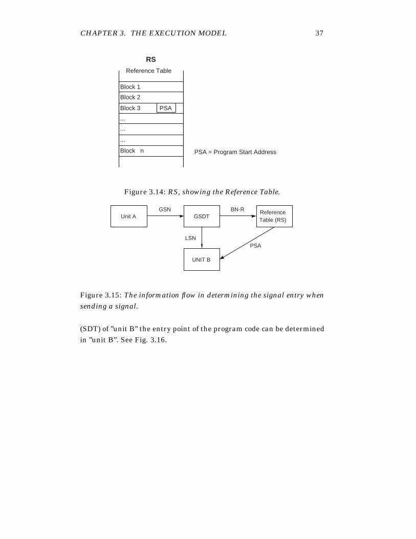
3.14 RS, showing the Reference Table. . . . . . . . . . . . . . . . 373.15 The information flow in determining the signal entry when
sending a signal. . . . . . . . . . . . . . . . . . . . . . . . . . 373.16 The consecutive order of handling a signal sending. . . . . 383.17 Show how addressing to DS is performed in RS. BSA points
to the starting point of BAT . . . . . . . . . . . . . . . . . . 40

vi
3.18 Different types of system restart. . . . . . . . . . . . . . . . . 433.19 The intensity counter. . . . . . . . . . . . . . . . . . . . . . . 443.20 Different levels of recovery after a detected software error. . 443.21 Data security of different start/restart types. . . . . . . . . 45
5.1 The compound statement expressed in natural semantics. . 535.2 The compound statement expressed in structural opera-
tional semantics. . . . . . . . . . . . . . . . . . . . . . . . . . 545.3 The compound statement expressed in denotational seman-
tics. . . . . . . . . . . . . . . . . . . . . . . . . . . . . . . . . 555.4 The compound statement expressed in a axiomatic seman-
tics style. . . . . . . . . . . . . . . . . . . . . . . . . . . . . . 56
6.1 The different stores in the central processor (CP). . . . . . . 596.2 A simplified figure of the job buffers in the PLEX/AXE
environment. (See also Fig. 3.10) . . . . . . . . . . . . . . . 606.3 The FIFO-semantics of the job buffers. . . . . . . . . . . . . 606.4 Organization of the job buffers. NOTE: The pointer regis-
ters, W8-W9, are treated as one register (and referred to asPOINTER B0). This is due to the fact that the register inW9 is only used when a pointer is too large to fit only inW8. In this case, the pointer will be split up and placed inW8 with its first half, and in W9 with its second half. . . . . 61
6.5 PLEX iteration statements - a comparison. . . . . . . . . . . 706.6 The process of finding the receiver of a buffered signal. (Re-
peated from Section 3.2.3, Fig. 3.12.) NOTE: The processis similar for direct signals, except that they are not in-serted in a Job Buffer. (See also Figure 6.4 for a detaileddescription on the organization of the job buffers.) . . . . . 85

List of Tables
6.1 Priorities and meaning of the PLEX operators. Prioritiesare numbered from the highest (1) to the lowest (8). . . . . . 66
6.2 A summary of the semantic functions defined and used inChapter 6 (and in Appendix A). . . . . . . . . . . . . . . . . 74
6.3 The semantics of ”arithmetic” expressions. . . . . . . . . . . 766.4 The semantics of ”boolean” expressions. (See also, Table
6.1 where the different operators, as well as their meaning,are described.) an represents a field-expression whereas tn
represents a string. . . . . . . . . . . . . . . . . . . . . . . . 776.5 The function APZ which fetches the first ”ready-job” with
highest priority. . . . . . . . . . . . . . . . . . . . . . . . . . 94
Chapter 1
Introduction
1.1 Background and Problem Definition
The programming language PLEX (Programming Language for EXchan-ges) is a pseudo-parallel and event-based real-time language developedby Ericsson. The language is designed for telephony systems and usedin central parts of the AXE switching system (from Ericsson). The lan-guage has a signal paradigm as its top execution level, and it is event-based in the sense that only events, encoded as signals, can trigger codeexecution. The term pseudo-parallel has arisen due to the fact that aPLEX program file consist of independent sub-programs (which will bediscussed in Section 3.1, and Fig. 3.3), in combination with an execu-tion model (Fig. 3.11) where new jobs are spawned and put in differentqueues, called job buffers, for later execution.
The language has been continuously evolving since the 1970’s whenit was originally designed. But in parallel with this, attempts have beenmade to introduce more ”modern” languages like C++ for instance, orspecification languages like standard SDL, and let the system executethis code as well as PLEX code. However, most of these attempts havefailed and considerable money has been spent. It is probable that thefailure is due to properties of the language and its execution model, i.e.the semantics of the language has not been paid enough attention. Forexample, to use SDL successfully, the unique semantics of PLEX wereconsidered in creating an extension to SDL, called SDL-10 which couldthen be code generated to PLEX.
Until now, the semantics for PLEX has been defined through its im-
CHAPTER 1. INTRODUCTION 2
plementation. A formal semantics for the language can serve as an ex-act documentation, which could be referred to when the implementationis updated (e.g., when a new hardware platform is introduced).
This report should also be seen in a further perspective, where theaim is to extend and modify the language with a possibility to run in amulti-processor environment, see Fig. 1.1. This could already be donetoday due to the modular structure of the language, but as shown byLindell [Lin03], there are problems that need to be solved.
1.2 Limitations
This report will focus on the basic concepts of signals since this is con-sidered to be the most important aspects of the language, and the partsthat most significantly differentiate PLEX from other languages. It willgive an operational semantics for the individual PLEX statements, aswell as for sequences of statements. However, the semantics for se-quences of statements is restricted to well-formed constructs (which willbe defined in Section 6.19).
1.3 Aim
The aim of this report is to give a semantic definition of the most im-portant parts of PLEX, mentioned in Section 1.2. With this in hand,a formal basis for further investigations and comparisons with otherlanguages is provided since the meaning of a (PLEX)program has beengiven a semantic definition. The semantics will also reveal ambiguitiesand prevent ”ad hoc” solutions when the language is moved to a newhardware platform.
A second aim is to form the basis for further investigations in thedirection of executing PLEX in a multi-processor environment.
1.4 Organization
This report is structured in two main parts:
• Part I includes the Technical Report ”The Execution Model ofAPZ/PLEX - An Informal Description” by J. Erikson and B Lin-

CHAPTER 1. INTRODUCTION 3
dell [EL02]. This part serves as an introduction to the executionmodel of PLEX for the reader not familiar with the language andits environment1. This part could be skipped, without any loss, bythe reader familiar with PLEX.
• Part II is the main part of this report. This part deals with the se-mantics for PLEX. Chapter 5 serves as an introduction to semanticnotation and describes the most common frameworks. Chapter 6could be seen as the main chapter of this report, since the seman-tics for PLEX is defined here. The semantics is developed through-out the chapter, when we look at the different statements in thelanguage. Appendix A then summarizes the semantics that aredefined in Chapter 6.
"A StructuralOperational
Semantics for PLEX"(Erikson)
"The Execution Model ofAPZ/PLEX - An Informal
Description"(Erikson & Lindell)
"Analysis of reentrancyand problems of data
interference in the parallelexecution of a multiprocessor AXE-APZ
system"(Lindell)
PLEXExtensions and
Modifications for parallelexecution
Figure 1.1: This report and its context.
1Also, a general survey of PLEX as well as of the AXE switching system can be foundin [AGG99]

Part I
The Execution Model ofAPZ/PLEX

Chapter 2
The AXE System and thePLEX Language
2.1 The AXE System
The AXE telephone exchange system from Ericsson, developed in itsearliest version in the beginning of the 1970s, is structured in a modularand hierarchical way. It consists of the two main parts:
APT: The telephony or switching part
APZ: The control part including central and regional processors
which both consist of hardware and software. The two main parts aredivided into subsystems.
A subsystem is divided in function blocks. Function blocks consistof function units which is either a central software unit or a hardwareunit, a regional software unit and a central software unit. The originalstructure of the system is shown in Fig 2.1.
Somewhere around 1994-95, the concept of Application Modularity(AM) was integrated into the system. This will be discussed in Section2.1.2
2.1.1 Central- and Regional Processors
The hardware aspects that is of interest in this report is the distinctionbetween Central- and Regional Processors. This is because different

CHAPTER 2. THE AXE SYSTEM AND THE PLEX LANGUAGE 6
System Level 1
System Level 2
Subsystem
Function Block
Function Unit
CPS NMS
LIC LIR LIUCJU
AXE
APZ APT
MAS FMS SSS GSS
CJ KR LI
APT - Telephony/Switching part APZ - Control part including central and regional processors
as well as operating system CPS - Central Processor SubsystemMAS - Maintenance Subsystem
AMAM . . .
Figure 2.1: The (original) hierarchical structure of the AXE system. (Theparts that will be of interest in this report is marked with bold text.)
forms of interwork is performed between different kinds of processors.The distinctions are briefly discussed in this subsection and explainedin more detail in Section 3.1.
Regional Processor (RP): There are several regional processors inan AXE system. The main task of a regional processor is to relievethe central processor by handling small routine jobs like scanningand filtering.
Central Processor (CP): This is the central control unit of the sys-tem. All complex and non-trivial decisions are taken in the centralprocessor. This is the place for all forms of non-routine work. Thework of the processor can be separated into two specifically dis-tinct parts, namely instruction execution and job administration.Instruction execution means handling of uninterrupted sequencesof operations where the work consists of address table look-up andcalculations, plausibility checks, storage accesses and data manip-ulations. The job administration mainly consists of signal han-dling, signal conversion and signal buffer handling. The execution

CHAPTER 2. THE AXE SYSTEM AND THE PLEX LANGUAGE 7
of instructions is a single-stream work by nature, whereas the jobadministration to a great extent is a question of prioritized jobqueues (Section 3.2) and transfer of signal data.
The CP is always duplicated. The two sides work in parallel, per-forming exactly the same operations. During normal operation,one CP is executive and the other is stand-by. A continuous checkis made to ensure that both processors reach the same result - Ifthey don’t, some form of recovery action is performed (Section 3.4).The CP duplication also enables function changes (installation ofnew software versions) while the exchange is in an operationalmode by first installing new software on the stand-by side andthen change the executive and stand-by order between the proces-sors. As a last step, the new software is installed on the formerexecutive (now stand-by) side.
The CPs store all central software and data. The CP memory con-sists of the register memory and the different stores. Programsare stored in the program store (PS) and data is stored in the datastore (DS). The reference store contains information about whereto find the different programs and data, Fig. 2.2.
Program Store
PS
Reference Store
RS
Data Store
DS
Figure 2.2: Stores in the central processor (CP). (The interaction betweenthe different stores are covered in Section 3.3.)
2.1.2 The Application Modularity (AM) Concept
The AXE Source System is a number of hardware and software re-sources developed to perform specific functions according to the cus-tomer’s requirements. It can be thought of as a ”basket” containingall the functionality available in the AXE system. Over the years, new

CHAPTER 2. THE AXE SYSTEM AND THE PLEX LANGUAGE 8
source systems has been developed by adding, updating or deleting func-tions in the original source system. But in the 1980’s, the developmentof the AXE system for different markets (US, UK, Sweden, Asia, etc.)has led to parallel development of the source system since functionalitycould not easily be ported between different markets.
The solution to this increasing divergence was the Application Mod-ularity (AM) concept, which made fast adaption to customer require-ments possible. The AM concept specifically targeted the following re-quirements:
• the ability to freely combine applications in the system,
• quick implementation of requirements, and
• the reuse of existing equipment.
The basic idea is to gather related pieces of software (and hardware)into something called Application Modules (AMs). Different telecomapplications, such as ISDN, PSTN (fixed telephony), and PLMN (PublicLand Mobile Network), are then constructed by combining the neces-sary AMs. The idea is described in Fig. 2.3, where it is also shown thatdifferent AMs can be used in more than one application.
AXE
APTAPZ
Separatetelecommucinationapplications
Aplication Modules (AMs)shared between differentapplications
ISDN PSTN PLMN
AM AMAMAMAMAM
Figure 2.3: The AM concept incorporated into the AXE system.

CHAPTER 2. THE AXE SYSTEM AND THE PLEX LANGUAGE 9
The introduction of the AM concept ended the problem with paralleldevelopment of different source systems. Instead, with AMs as buildingblocks, the required exchange was constructed by combining the neces-sary AMs into an exchange with the required functionality (i.e., withthe necessary applications).
2.1.3 Input and Output statements
An AXE exchange needs to communicate with its environment and itsoperation and maintenance (O&M) staff. Some typical situations couldbe the following:- An exchange technician changes subscriber categories, replaces de-vices or connects new subscribers.- The exchange informs the O&M staff of important events, e.g., if anRP is blocked due to a fault. In other words, the I/O statements are animportant part of the recovery mechanism. (See Section 3.4.)- Input/output includes certain routine tasks to, e.g. dumping data on ahard disk.There is a large number of I/O devices used; alarm and hard copy print-ers, display units, work stations and PC’s, magnetic tape drivers, hardand flexible disks.
Before communicating with an I/O device, the PLEX program hasto seize the device. Likewise, the device has to be released when thecommunication ends. This guarantees exclusive access to the device.All I/O devices are connected to a support processor (SP), and functionblocks that receive or send information via the I/O system are calleduser blocks. Fig. 2.4 shows the interaction between the I/O system anda user block. When seizing an I/O device, the I/O system assigns a freeline buffer and a free analysis buffer (see Fig. 2.4) to this device. Thesebuffers temporarily store the I/O text. The analysis buffer handles inputfrom the I/O device, and the line buffer handles output.
The basic (PLEX) statements for transferring information betweenthe buffers and the I/O device, and between the buffers and the userblocks are:- FETCH: transfer information from the analysis buffer to the user block.- INSERT: transfer information from the user block to the line buffer.- WRITE: orders the I/O system to print out the text in the line buffer to

CHAPTER 2. THE AXE SYSTEM AND THE PLEX LANGUAGE 10
SP
Line Buffer72 Characters
Analysis Buffer144 Characters
I/O System
UserBlock
2 Insert
3 Write
4 Read
1
1 Fetch23
4
Program Store
I/O device
Figure 2.4: The I/O system and its communication with the environ-ment.
an I/O device.- READ: transfer information from the I/O device to the analysis buffer.Again, see Fig. 2.4.
Typically, I/O communication starts with the operator entering acommand on an I/O device. The command is received by the I/O sys-tem and delivered to the software unit where it has been defined by theprogrammer. A command is received in a program (i.e., a software unit)in the same way as a signal (Section 3.1) but the command receivingstatement must be preceded by the keyword COMMAND to indicate thatthis is a statement used by the I/O system.
2.1.4 Load, Reload and Dump
An AXE exchange may exist for up to 40 years, which implies certainrequirements regarding the operation and maintenance of the software.The terms Load, Reload and Dump are covered in this section sincethey will be used in this report when we discuss variables (Section 2.2.3)and software recovery (Section 3.4).
When all the software blocks have been written and compiled, theprograms and data, initial and exchange, are written, dumped, to a

CHAPTER 2. THE AXE SYSTEM AND THE PLEX LANGUAGE 11
magnetic tape which is loaded into the exchange. This process is calledinitial loading. On loading of new blocks, or new revisions of existingblocks, an incremental re-linking occurs, as well as an initialization ofdata store variable values, if required according to their given variableproperties1. A DCI (Data Conversion Information) is written for eachblock being loaded to specify the data initialization between the old (ifexisting) and new blocks. During the function change process (Section2.1.1) the new block can get its new value from either of the followingthree ways:- Get value from data sector2.- Get value from DCI.- Get value from existing software.
In the case of system failure where a system restart3 has been per-formed, software backup copies are reloaded into the exchange. Whenreloaded, some variables will receive reload values from the magnetictape, whereas other variables will not have values until the programis executed by a signal4. Whether or not a variable receives a reloadvalue is determined by the variable properties set by the designer. Thisis covered in Section 2.2.3.Reloading means that the contents of DS (i.e., only RELOAD declaredvariables) are reloaded into the exchange again. If a change has oc-curred in PS and RS, they will be reloaded as well.
The contents of Program-, Reference- and Data store are regularlysaved to a hard disk (or a magnetic tape). This process is called dumpand enables the reload action described above.
2.2 Programming Language for EXchanges
Programming Language for EXchanges (PLEX) is designed by Ericssonand used to program telephony systems. It lacks common statementsfrom other programming languages such as WHILE loops, negative nu-meric values and real numbers. These are not needed in a telephony
1Variable properties is covered in Section 2.2.32The data sector is mentioned in Section 2.2.13The system restart process is explained in Section 3.44Signals are examined in Section 3.1

CHAPTER 2. THE AXE SYSTEM AND THE PLEX LANGUAGE 12
exchange system. The language was designed and developed in its firstform in the 1970s and extended in 1983. The version under considera-tion in this report, PLEX-C, is used in the AXE central processors (seeSection 2.1.1). Other languages used in the AXE system are shown inFig. 2.55. The reason for developing a new language for the AXE sys-tem was that no other languages under consideration fulfilled Ericsson’srequirements.
Some important characteristics of the language are listed below:
• PLEX is an event-based language with a signaling paradigm asthe top execution level. Only events can trigger code executionand events are programmed as signals. A typical event is when asubscriber lifts the phone to dial a number.The execution model is described in Chapter 3 and signals in Sec-tion 3.1.
• The signals are executed on one of four priority levels (explainedin Section 3.2), which results in very little overhead when a higherlevel interrupts a lower since each priority level has its own regis-ter set.
• Jobs (Section 3.2.1) at the same level are ”atomic” and can neverinterrupt each other.
2.2.1 The structure of a PLEX program
When we talk about a PLEX program, or a PLEX program file, we meanthe PLEX file that specifies a function unit (Section 3.0.7). This docu-ment, the Source Program Information (SPI), shown in Fig. 2.6, consistsof the following main parts:
• The Declare sector, which contains the variable and constant dec-larations that are used in the program sector. Variables with theproperty DS, Data Store, (Section 2.2.3) will exist beyond the exe-cution of subprograms.
5As could be seen in Fig. 2.5, there is another dialect of PLEX (PLEX-M). However,these dialects are similar, and when we talk about PLEX in this report, we mean thedialect used in the central processors, i.e, the PLEX-C dialect.

CHAPTER 2. THE AXE SYSTEM AND THE PLEX LANGUAGE 13
EMRPD
EMRP
EM
RPG
CP
STR STC RPD RP
GARP
C/C++
Plex-MASM 6809
ASM 6809 ASM 6809 C/C++
ASA 21RASA 210R
Plex-CASA 210C
EMRPD - Extension Module Regional Processor Digital EMRP - Extension Module Regional Processor STR - Signaling Terminal Remote STC - Signaling Terminal Central RPD - Regional Processon Digital RP - Regional Processon CP - Central Processon EM - Extension Module RPG - RP with group switch interface GARP - Generic Application RP
C/C++
C/C++
Figure 2.5: The different languages used in different parts of the AXEsystem

CHAPTER 2. THE AXE SYSTEM AND THE PLEX LANGUAGE 14
• The Parameter sector, where specific AXE parameters are placed.These parameters are not local to a block, and permit global accessfrom all parts of the exchange. They can be changed by customerssince they are placed in an SQL database.
• The Program sector contains the executable statements, i.e., thePLEX source code that will run in the exchange. This sector isnormally divided in several subprograms (explained in Section 3.1and Fig. 3.3).
• The Data sector: Some variables, i.e. Data Store variables, needsto have initial values when the program (i.e., the SPI) is loadedinto the exchange6. These initial values can be provided in thedata sector. Also, the position, i.e. the base address, of stored vari-ables in memory can be allocated in the data sector. This enablesa faster function change (briefly described in Section 2.1.1).
• The ID sector is used for internal documentation only.
The SPI is compiled together with the following documents7:- The Signal Survey, SS, which is a list of all the different signals thatone function unit (i.e., the function unit specified in the SPI) receivesand sends. There is one SS per function unit. There is no informationabout senders and receivers in the SS, this information is added laterduring loading.- The Signal Description, SD. The function blocks and function unitscommunicate with signals (Section 3.1). The SD describes the purpose,type and data of one signal. SDs are stored in separate signal handlinglibraries.
2.2.2 Records, Files and Pointers
Records collect variables that describe properties of a group of items,for instance, calls or subscribers8. Record variables may be stored field,symbol or string variables (Section 2.2.3). Variables in a record may
6The initial loading is described in Section 2.1.4.7The different steps of the compilation process, as well as the PLEX compiler, is
described in [AE00]8A (PLEX) record is similar to a struct in C.

CHAPTER 2. THE AXE SYSTEM AND THE PLEX LANGUAGE 15
DOCUMENT KRUPROGRAM; DECLARE; : : END DECLARE; PARAMETER; : : END PARAMETER; PROGRAM; PLEX; : : END PROGRAM; DATA; : : END DATA; END DOCUMENT; ID KRUPROGRAM TYPE DOCUMENT; : : END ID;
Figure 2.6: Structure of the SPI, i.e., a PLEX program file.
be indexed or structured, and they are called individual variables. DS(Data Store, described in Section 2.2.3) variables that are not part of arecord, are known as common variables.
A File is a set of records. One file consist of one or more records, allwith the same individual variables.
Pointers address the relevant record in a file. In PLEX, pointersare simply record numbers. The records in a file are numbered, andthe value of the pointer is the number of the current record. In otherwords, pointers in PLEX are not similar to pointers in C and can notbe manipulated in the same way. Fig. 2.7 shows an example file withits records and a pointer. The number of records in a file may be fixedor changeable. A fixed size is specified in the Data sector of the SPI(Section 2.2.1), while alterable file sizes are set by commands (Section2.1.3).
2.2.3 Variables
Depending on how variables is to be treated at a software error and afollowing recovery action, the PLEX designer can assign different prop-erties to the variables. This is to be covered in this section.

CHAPTER 2. THE AXE SYSTEM AND THE PLEX LANGUAGE 16
n
43
21
SUBNUMBER
NAME
STATE
0POINTER
Figure 2.7: An example file with n records and a pointer with the currentvalue 2.
There are three different data types in PLEX:- Field variables for numeric information. They contain non-negativeintegers only. (Negative integers are not needed in the AXE system.)- Symbol variables for symbol information, e.g., IDLE, BLOCKED, BUSY,etc.- String variables store text strings.These data types (variables) can be stored or temporary.
• The value of a temporary variable exists only in the Register Mem-ory (RM - internal CP registers) and only while its correspondingsoftware is being executed. Variables are by default temporary.
• Stored variables are stored in the Data Store (Fig. 2.2), loadedinto a register in the RM for processing and then written backto the DS. Thus, its value is never lost, even if the program isexited and re-entered later. DS variables are also a natural way tocommunicate between different forlopps9.
It is the stored variables that may be assigned the different propertiesalready described. These properties are DS, CLEAR, RELOAD, DUMP,
STATIC, BUFFER and COMMUNICATION BUFFER. The properties willall be described in this section.
9Forlopps are explained in Section 3.4.1

CHAPTER 2. THE AXE SYSTEM AND THE PLEX LANGUAGE 17
From a storage point of view, the variables can be divided into thefollowing types: Temporary and stored have been described above. Thethird category is the buffers. Buffer variables10 are allocated dynami-cally in an area reserved for dynamic buffers by using an allocate state-ment. The size of the buffers can be specified static (COMMUNICATIONBUFFER) or dynamic BUFFER. The fixed size is specified in the Declaresector (Section 2.2.1) while the dynamic size can be set in the Programsector. The dynamic buffers are slower than the static since they mustbe administered dynamically. These categories are pictured in Fig. 2.8together with its properties.
VARIABLES
REGISTER-ALLOCATED VARIABLES(Temporary variables)
MEMORY-ALLOCATED VARIABLES(DS & BUFFER)
PERMANENTLYALLOCATED VARIABLES (DS)
DYNAMICALLYALLOCATED VARIABLES (BUFFER)
STATIC
CLEAR
RELOAD
DUMP
Field
Var
Var
Symbol
Var
String
DUMP
Field
Var
Figure 2.8: Variables and properties (from a storage point of view).
Under normal circumstances, the exchange starts the (application)software and it never stops. After serious errors, however, the APZ (i.e.,
10Buffer variables are similar to the array structure in C.

CHAPTER 2. THE AXE SYSTEM AND THE PLEX LANGUAGE 18
the operating system part) stops the program execution and restartsthe software. The following properties describe the variable behavior atstart or restart:
• CLEAR - ”Clearing at start/restart”Field variables are set to zero; symbol variables to the first valuein their declaration list.
• RELOAD - Loading at ”restart with reload”The variable value is reloaded from tape/hard disk to ensure thatthe values before and after the ”restart with reload” are the same.
• DUMP - ”Dumping at restart”.This property is used for testing and tracing purposes.
• STATIC - When a software unit in an operating exchange is to beupdated, a function change takes place. Remember from Section2.1.1 that the CP is always duplicated. This means that new soft-ware can be installed while the exchange is running. A STATIC
declared variable means that the variable value is not updatedwith a new software version.
Not all combinations of the variable properties are possible (i.e., legal).Fig. 2.9 contains a table listing all valid combinations of variables andproperties.
2.2.4 Data Encapsulation
All variables and constants declared in the Declare sector of the SPI,see Section 2.2.1, have their scope inside the software unit specified. Allsubprograms (Section 3.1) of that SPI can access these variables andconstants. Subprograms not part of that function unit cannot accessthese variables and constants.

CHAPTER 2. THE AXE SYSTEM AND THE PLEX LANGUAGE 19
Field Variable
String Variable
Symbol Variable
DS DS DUMP DS STATIC DS RELOAD DS RELOAD DUMP DS RELOAD STATIC
DS CLEAR DS CLEAR DUMP
BUFFER BUFFER DUMP
Temporary
Yes
Yes
Yes No
NoYes(1)
Yes No
(1) Except for one- and two-dimensional arrays
Figure 2.9: Permitted combinations of variable properties and variabletypes.
SignalENTRY 1
SignalENTRY 2
SignalENTRY 3
SignalENTRY 4
... ... ...Signal
ENTRY n
Variable A
DATACommon Data Storagefor all Variables in allentries of the whole
Block
Figure 2.10: The structure of a software unit (block). The possibility ofseveral sub-programs accessing the same data within the block is shown.All sub-programs (signal entries) can access all DS variables inside thesame block (except for individuals that are DS variables inside a record).This conveys a DS variable can be used as a communication channelbetween all sub-programs inside the same software unit.

Chapter 3
The Execution Model
A brief discussion of the execution model has already been given in Sec-tion 2.2 and we continue and deepen the discussion in this section. Wefirst briefly discuss PLEX structure, operating system requirements,function blocks and application system before we look deeper at pro-gram interwork (i.e, signals), Section 3.1, and job buffers, Section 3.2,both central concepts in the PLEX/APZ environment.
3.0.5 PLEX structure and OS requirements
PLEX is an asynchronous concurrent event based real-time languageand, as stated in Section 2.2, it has a signaling paradigm as the topexecution level which means that only events can trigger code executionand these events are programmed as signals. Signals will be furtherexplored in Section 3.1. The main task of an operating system that is torun PLEX, is to buffer incoming signals and start their execution in theright signal entry statement.
3.0.6 Software Units
In large software systems, such as a telecommunication system, thereis a need to group code into modules, for example, to control a certainhardware, or to implement in software add-on functionality. A SoftwareUnit is a quantity of PLEX code for the different jobs1 needed for sucha module, called a function. A Unit can not access data in another unit,
1Jobs are covered in Section 3.2.1.

CHAPTER 3. THE EXECUTION MODEL 21
Event
Hardware
Hardware
RP(D)
EMRP(D)
unit structure
function block
RP-CP signal
SST
SDTDATAunit }
}
code
enter
exitsend
effect
aptapz signal interface
forlopp
forloppmanager
restartcode
restart signal
cp-cpsignal
apz
apt
Central Processor (CP)
APT applicationsystem
APZplatformsystem
Figure 3.1: APT Application system.

CHAPTER 3. THE EXECUTION MODEL 22
i.e, a unit has data encapsulation (see Section 2.2.4).
3.0.7 Function Blocks
A function block is a software unit by itself or a software unit in theCP with the associated software unit in the EMRP or RP and possiblyassociated hardware needed to implement a function.
If we relate the function blocks to the AM concept, described in Sec-tion 2.1.2, it should be pointed out that an AM is not a PLEX languageconstruct. From a PLEX language point of view, each AM and the com-mon resources can be seen as a collection of blocks. Signals betweenAMs and to/from the common resources are gathered into standard in-terfaces.
3.0.8 Application System
An application system is a group of function blocks that interwork to-gether to form a complete application, such as the control of a certaintelephone exchange, see Fig. 3.1. All the signals and units of the partof the application system hosted on a certain processor take part in a”linking” process. (For units written in PLEX-C, the host is the CP.)The linking process resolves that signals sent from a certain unit aredirected to the right entry point in the right unit.
3.1 Program Interwork - Signals
A signal is an externally defined language element in PLEX for the in-terwork between software units. A signal can be described as a messagewithin one or between two software units or as an asynchronous (oneway) function call, i.e., it is signals that perform the communication be-tween different function units. Signals can be classified in numerousways (Section 3.1.1, 3.1.2, 3.1.3 and 3.1.4) but the main distinctionis between direct and buffered signals (Section 3.1.1). A direct signal issimilar to a jump from one function unit or program to another, whereasa buffered signal is more like a fork2 system call except that the ex-
2fork is a nonANSI C function that ”copies the current process and begins executingit concurrently”, [KP96]. The execution will then continue in this newly created ”child-
CHAPTER 3. THE EXECUTION MODEL 23
ecution continues in the ”parent process” whereas the ”child process”is put in the job queue (Section 3.2) for later execution. In this way,after the sending of the buffered signal, the two execution paths areindependent parallel threads, unsynchronized with each other. The dif-ference is explained in more detail in Section 3.1.1, but we already statethat buffered signals is the ”norm” and that the classification referredto only applies to CP-CP signals. CP-RP and RP-CP signals are alwaysbuffered.
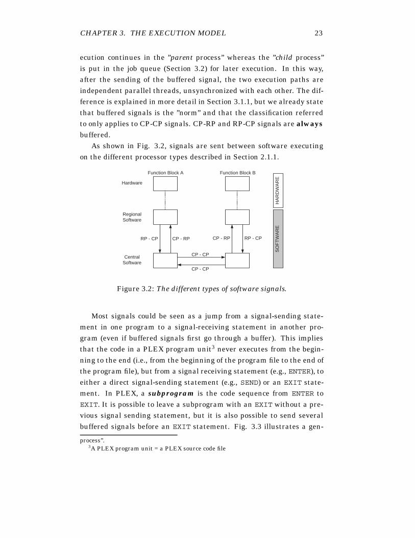
As shown in Fig. 3.2, signals are sent between software executingon the different processor types described in Section 2.1.1.
RP - CP CP - RP RP - CPCP - RP
CP - CP
CP - CP
Function Block A Function Block B
Hardware
RegionalSoftware
CentralSoftware
HA
RD
WA
RE
SO
FT
WA
RE
Figure 3.2: The different types of software signals.
Most signals could be seen as a jump from a signal-sending state-ment in one program to a signal-receiving statement in another pro-gram (even if buffered signals first go through a buffer). This impliesthat the code in a PLEX program unit3 never executes from the begin-ning to the end (i.e., from the beginning of the program file to the end ofthe program file), but from a signal receiving statement (e.g., ENTER), toeither a direct signal-sending statement (e.g., SEND) or an EXIT state-ment. In PLEX, a subprogram is the code sequence from ENTER toEXIT. It is possible to leave a subprogram with an EXIT without a pre-vious signal sending statement, but it is also possible to send severalbuffered signals before an EXIT statement. Fig. 3.3 illustrates a gen-
process”.3A PLEX program unit = a PLEX source code file

CHAPTER 3. THE EXECUTION MODEL 24
eral program divided into subprograms. Note that since programs writ-ten in PLEX do not normally execute from start to end, or in any order,it can not be assumed that the program in Fig. 3.3 receives SIGNAL1before or after SIGNAL3, or SIGNAL4 before or after SIGNAL6. Thiscan result in unpredictable values of stored variables.
PROGRAM; PLEX; ENTER SIGNAL1; .... SEND BUFFERED SIGNAL2; .... EXIT;
ENTER SIGNAL3; .... SEND DIRECT SIGNAL4;
CUSELESS = 0;
ENTER SIGNAL5; .... SEND BUFFERED SIGNAL6; .... SEND DIRECT SIGNAL7;
ENTER SIGNAL8; .... EXIT;
.... END PROGRAM;
a subprogram
a subprogram
a subprogram
a subprogram
Figure 3.3: A PLEX program file divided in subprograms. Note that theassignment CUSELESS = 0; will never be executed since it is placed be-tween an exit and an enter statement. (See also Fig. 2.6 where a completeprogram file is described.)
Since the exchange handles several calls simultaneously while theCP can only execute one program at a time, the CP must queue thesignals somewhere. This is done in job buffers, a job table or in timequeues and this will be explored in Section 3.2.
As was said earlier there are different parameters that describe thesignal properties of a CP-CP signal. Three groups classify these prop-erties and each signal has one property from each group. Each group isdescribed below and all possible combinations is shown in Fig. 3.7.

CHAPTER 3. THE EXECUTION MODEL 25
3.1.1 Direct and buffered signals
As was stated in Section 3.1, the main distinction between (CP-CP) sig-nals is whether they are direct or buffered. Buffered signals start a newjob, whereas direct signals continue the current job. (Jobs are coveredin Section 3.2.1). That is, they are handled differently in the executionmodel.
Direct signals reach the receiving block immediately, they could beseen as direct jumps to another unit. By using direct signals, othersignals have no possibility of coming-in-between, i.e., the programmerretains control over the execution. However, direct signals are normallyonly allowed to be used in very time-critical program sequences, such ascall set-up routines.
With buffered signals, it is not predictable when the signal reachesthe receiving block. Direct and buffered signals are illustrated in Fig.3.4.
Unit A Unit B
A Direct Signal
Unit A Unit B
A Buffered Signal
Job Buffer
Figure 3.4: Direct and buffered signals.
3.1.2 Unique and multiple signals
This distinction concerns the number of receivers of the signal. A uniquesignal can only be received in one particular block, while a multiplesignal can go to any block as shown in Fig. 3.5. However, it is notpossible to send a multiple signal to more than one block simultaneouslywhich means that a multiple signal does not perform multicast4. Buteven if a multiple signal can go to any of the receiving blocks specified in
4Multicast: Send once - received by all

CHAPTER 3. THE EXECUTION MODEL 26
the Signal Survey5, the signal sending statement must always containone (and only one) receiver of the multiple signal.
Unit A Unit B
A Unique Signal
Unit D
Unit C
Unit B
Unit A
A Multiple Signal
Figure 3.5: Unique and multiple signals.
3.1.3 Single and combined signals
The third distinction concerns whether the sending block expects ananswer. Combined signals demand an immediate answer, while singlesignals do not require such feedback. For this reason, combined signalscan never be buffered (as shown in Fig. 3.7). Instead, they behavelike direct jumps from one unit to another. When the execution in theother unit (the receiver of the signal) finishes, execution jumps back tothe originating unit. Combined signals are always direct signals, whichmeans that execution continues without interrupt and all other signalshave to wait. Fig. 3.6 illustrates these kind of signals.
When discussing the sending and receiving of combined signals, onewill also mention forward and backward signals. A communication be-tween two parts6 is always initiated by one of the parts. The initiatingpart is sending the forward signal whereas the part that replies to thecall is sending the backward signal. This is pictured in Fig. 3.8.
5The Signal Survey is described in Section 2.2.16Which, in our target domain, is the sending and receiving of signals between func-
tion blocks.

CHAPTER 3. THE EXECUTION MODEL 27
Unit A Unit B
A Single Signal
Unit A Unit B
Combined Signals
Figure 3.6: Single and combined signals.
Signal Type BufferedDirect
Single
Combined
unique
multiple
unique
multiple
X
X
X
X
X
X
Figure 3.7: Possible properties for CP-CP signals. X indicates a le-gal/possible combination, shaded with Grey indicates an illegal alter-native. NOTE: A combined backward signal can not be multiple sincethis signal is an answer (i.e., an acknowledgment) to a ”caller” and musttherefore return to the ”caller” and nobody else.
SEND Signal-A(Forward)
RETRIEVE Signal-A(Backward)
RECEIVE Signal-B(Forward)
RETURN Signal-B(Backward)
Block A
RECEIVE Signal-A(Forward)
RETURN Signal-A(Backward)
SEND Signal-B(Forward)
RETRIEVE Signal-B(Backward)
Block B Time
Figure 3.8: Forward and Backward signals.
CHAPTER 3. THE EXECUTION MODEL 28
3.1.4 Local and Non-local signals
In the beginning of Section 3.1, we said that signals are used ”for theinterwork between software units”. But signals can also be used forthe interwork between different parts of the same software unit. Thesesignals are called local signals, since they are local to the software unitthey belong to. I.e., the recipient resides in the same software unit.(Consequently, all other signals are called non-local signals.
The behavior of a local signal is similar to that of a GOTO statementsince they result in direct jumps to the recipient. (And in that sense,they can be regarded as direct signals.)
Whether a signal is local or not, is specified in the Signal Description(which was briefly explained in Section 2.2.1, and covered in more detailin Appendix B). The distinction between local and non-local signals isof importance in, for instance a semantic framework for PLEX.
3.1.5 Signals and Priorities
Every signal that is sent in the system is assigned a priority level, A -D. The priority level is of importance when the signal is to be buffered(Section 3.2), and it tells the ”importance” of the source code that is trig-gered to execution by the signal. The priority of each signal is specifiedin the corresponding Signal Description.
3.1.6 Signals and Data
Signal Data are variable values sent with a signal7. The data may con-sist of field variables, symbol variables, pointers, numerals, string ob-jects, buffer variables and field expressions. For single and combinedsignals, it is possible to send 25 signal data. The data is loaded to theregister memory in the central processor (see Section 2.1.1) if the signalis direct, or to the job buffer if the signal is to be buffered.
3.2 Jobs, Signal Buffers and Job Handling
In the following sub-sections, we will discuss the definition of a job (Sec-tion 3.2.1), the different ways of delaying/buffering a signal (Section
7This is similar to a call by value function call.

CHAPTER 3. THE EXECUTION MODEL 29
3.2.2) and, finally, how jobs are handled at runtime (Section 3.2.3).
3.2.1 What is a Job?
A job is a continuous sequence of statements executed in the processor.A job begins with an ENTER statement for a buffered signal and endswith an EXIT statement.
Between the ENTER and the EXIT statement, several buffered sig-nals (or no signals at all) may be sent. A job is not limited to one CPsoftware unit, several units and blocks can take part in a job.
A job does always have a single entry point but it may have multipleexit points.
In Section 3.1.5 we discussed the priority of a signal. In the followingsubsections, we will instead talk about the priority of a job. This makesense since it is more natural to look at whole jobs when discussingexecution of PLEX code, than it is to look at a single8 signal. The reasonis that a job includes the actual PLEX code that is triggered to executionby the signal, as well as the signal itself.
3.2.2 Signal Buffers
Some jobs in the AXE system are not time-critical and can wait to beexecuted, while others need to be executed immediately. The first caseholds for administrative jobs and the second case for jobs related to traf-fic handling (i.e., telephone calls9) and CP faults.
Buffered signals (which could be read as ”the start of a new job”)may be delayed using one of the following methods:
• Job Buffer: delays a signal until all ”older” jobs have been processed
• Job Table: sends signals at short periodic intervals
• Time Queue: delays signals by relative or absolute time
We will look further to these different ways of delaying a signal.8By single signals, we do not mean single signals as described in Section 3.1.3.9A normal load on the system is 200 telephone calls that is to be handled every
second. These jobs are all time critical and have the same priority, but the performancewould not be acceptable with a ”first-come-first-served” approach. A solutions is to usebuffered signals as a ”time sharing” mechanism.

CHAPTER 3. THE EXECUTION MODEL 30
Job Buffers: Job buffers are queues with a FIFO-semantics10. Thereare four buffers for CP-CP and RP-CP signals and one for CP-RPsignals; Job Buffer A, Job Buffer B, Job Buffer C and Job BufferD, all for CP-CP and RP-CP signals, where Job Buffer A has thehighest priority. Job Buffer R is the buffer for CP-RP signals.
The buffers carry the following type of tasks:Job Buffer A - urgent tasks of the operating system; preferentialjobs, e.g., errors in traffic equipment.Job Buffer B - telephone traffic.Job Buffer C - I/O communication. The command statement de-scribed in Section 2.1.3 is handled at this level.Job Buffer D - APZ routine self-tests.Job Buffer R - CP-RP signals queue in JBR, a buffer for signalssent from the CP to a RP.
The Job Table: The job table contains jobs executed at short periodicintervals, for instance, incrementing clocks for time supervision.The job table has higher priority than any of the job buffers. Sincethe possible execution time after a job table signal is very short,this signal only initiates a program sequence in the receiving block,which inserts a buffered signal in one of the job buffers. Thebuffered signal initiates the ”real” work in the program which froman application point of view, has the priority of the buffer it is in-serted in.
Time Queues: Time queues delay periodic and other jobs at longer in-tervals than the job table. There is one absolute time queue andthree relative ones. The absolute time queue stores the absolutetime for signal execution (month, day, hour and minute). Everyminute, the time queue compares this value with the system cal-endar. When there is a match, the signal is moved to one of thefour job buffers. The three relative queues have a counter for eachjob. Every 100 ms, 1 second and 1 minute, respectively, the timequeue receives a periodic signal from the job table and decrementsthe counter. If a counter reaches the value zero, the correspond-ing signal is forwarded to one of the job buffers. I.e., a signal that
10First In First Out

CHAPTER 3. THE EXECUTION MODEL 31
is fetched from a time queue is almost never executed at once11.Execution of the signal is performed when the operating systemfetches it from the job buffer it was inserted in.
Fig. 3.9 shows how a software unit sends a delayed (and multiple) sig-nal. The signal is first placed in a time queue and after that in a jobbuffer. After it is taken from the job buffer, the execution is started inthe receiving unit.
...Enter SigA
...
Unit B
...Enter SigA
...
Unit C
Time Queue Job Buffer
...Send SigA
...Delay 200ms
EXIT...
Unit A
Figure 3.9: Sending of a delayed (and multiple) signal. The signal issent from Unit A and received in Unit C but, as could be seen in thefigure, it is possible to receive the signal in Unit B as well if Unit B isspecified as the receiver by the PLEX designer.
3.2.3 Job Handling
The priorities at runtime correspond to the priorities among the jobbuffers (Section 3.2.2), as will be shown below.
As already stated, Section 3.2.2, depending on their purpose andtime requirements, jobs are assigned to certain priority levels - five dif-ferent levels exist. But the important thing, when discussing job pri-orities, is how different priority levels can interrupt each other and, ascould be seen in the following discussion, we could view the five differ-ent priority levels as only three if we take the possibility for one job topreempt another into consideration.
11The only exception is when the receiving job buffer (and every job buffer with higherpriority) is empty.

CHAPTER 3. THE EXECUTION MODEL 32
Tasks initiated by a periodic Job Table signal use the traffic-handlinglevel 1 (THL 1), JBA signals use traffic-handling level 2 (THL 2), JBBuse traffic-handling level 3 (THL 3), JBC use base level 1 (BAL 1) andJBD use base level 2 (BAL 2), see Fig. 3.10.
The Job Table has a higher priority than all the job buffers. JBA hasa higher priority than JBB, and so forth. The jobs in the job buffers areexecuted in order of priority - JBA is emptied before JBB, and so on.Data used in interrupted jobs stay in the processor register memory,and THL, BAL 1 and BAL 2 jobs have their own processor registers.That means all THL jobs share the same register buffers. Hence, no jobat one sub level of THL can interrupt a job at another sub level of THL,since they share the same set of registers and the temporary variableswould be destroyed otherwise.
I.e., jobs from the job table, JBA and JBB have to wait for each other,but all three can interrupt job from JBC and JBD. As BAL 1 and BAL 2have different register memories, JBC can interrupt JBD.
Job TableJBAJBBJBCJBDJBR
Job Buffers for CP-CPand RP-CP signals
Job Buffer for CP-RP signals
JBA - urgent tasks of the operating system: preferential trafficJBB - all other telephone trafficJBC - input/output to operator and I/O devicesJBD - APZ routine self-testJBR - signals from Central Processor to Regional ProcessorTHL - traffic-handling levelBAL - base level
THL 1THL 2THL 3BAL 1BAL 2
THL
Own processor registerOwn processor register
Shared processorregister
Figure 3.10: Job buffers and runtime priorities in the AXE system.
In some cases, however, it may be necessary to prevent the systemfrom interrupting an important task. For example, an operation andmaintenance (O&M, Section 2.1.3) routine at C-level (BAL 1) is writingto variables that are also accessed by traffic-handling routines at B-level(THL 3). In this situation, it is best to inhibit the interrupt function as

CHAPTER 3. THE EXECUTION MODEL 33
long as the writing at C-level is in progress. The interrupt function isinhibited by the DISABLE INTERRUPT statement and activated by theENABLE INTERRUPT statement.
We conclude this subsection with an exampel. Fig. 3.11 illustratesthe execution of several jobs. In the figure, the execution starts in block1 with the first job, proceeds in block 2 with the second job and finallyends in block 1 with the execution of the last job. Fig. 3.12 gives a closerlook of the link (into job buffers) and execute process.
If a new job enters an empty job buffer, the buffer sends an inter-rupt signal for that priority level. If the ongoing job has a lower prioritylevel, that job is interrupted. However, a job can not interrupt a job onthe same (or higher) priority level.
Timeblock 1 block 3block 2
enter
send
exit enter
send
send
exit enter
enter
send
exit
signal 1
signal 2
signal put injob buffer
signal 5
signal put injob buffer
signal put injob buffer
signal 3
signal 4exit
Figure 3.11: The execution model - Four jobs are executed. The processof transfering a buffered signal from the sending block to the receiving,via a job buffer, is shown in Fig. 3.12. NOTE the ”parallel” architecturethat could become real parallel execution.

CHAPTER 3. THE EXECUTION MODEL 34
(module)block A
Signal Number
1
5432
Link Signal Number
ENTER
EXITENTER
SEND siganlname
EXITENTER
EXIT
Signal Number 1
432 Block number of B
APZ
(module)block B
ENTER
EXITENTER
EXITENTER
EXIT
Hop address
SSTSST
SDTSDT
APZ - Operating System SDT - Signal Distribution Table SST - Signal Sending Table
Job Buffer
Signal Number
DataBlock Nr ofB
Figure 3.12: Linking and execution for a buffered signal in APZ. See alsoFig. 3.11. NOTE: The procedure is the same for direct signals except thatthey not are inserted in a Job Buffer.

CHAPTER 3. THE EXECUTION MODEL 35
3.2.4 Execution Time Limits
As stated in Section 3.0.5, PLEX is a real-time language. This meansthat a system programmed in PLEX is a real-time system12. When talk-ing about execution times limits, one always refer to the execution timeof a job. There are limits for the execution time, but this is not mea-sured in absolute times. Instead, there are programmer guidelines thatspecify how many lines of code that may be placed in a software unit (orunits) for one job.
3.3 Linking Encapsulation
All blocks used in the system are compiled separately and it is also pos-sible to ”load“ them separately, even at run-time. This process is calleda Function Change and it was described in Section 2.1.1. When do-ing a Function Change, the Signal-Sending Table (SST) and the Global-Signal Distribution Table (GSDT) has to be updated. The update hasto be done because all signal sendings has to look in the SST and theGSDT to find which signal to invoke.
When updating the tables, by the Rationalized Software Production(RSP) functionality, the (new) introduced signal is given a unique num-ber, the Global Signal Number (GSN). This number is stored in theGSDT as well as in the SST of the Function Unit (block) using this”new“ signal. The GSDT also stores Block Number Receiving (BN-R),(the unique number of the block receiving the signal) and the LocalSignal Number (LSN) which is the position holding the local relativeaddress of the entry point of the signal entry.
The Signal Distribution Table (SDT) is not updated, as the SDTholds the relative address to the signal entries inside the Function Unit.SDT is set with a local number in the object step (during compilation).
SDT: Contains the relative entry address, set during compilation, ofthe specific program sequences where signals are received.
SST: Contains the global signal number (GSN) of signals to invoke12And, as shown by Arnström et. al, the AXE system is classified as a soft real-time
system [AGG99].

CHAPTER 3. THE EXECUTION MODEL 36
SignalDistribution Table
(SDT)
Signal SendingTable (SST)
Program Code
PS
One function Unit(Block)
Figure 3.13: PS, showing SDT, SST and Program Code of one functionunit.
from function unit using ”this“ SST, created in the object step andchanged by the RSP.
GSDT: Contains the global signal number (GSN), the Block NumberReceiving (BN-R) and the Local Signal Number (LSN).
In DS, values are stored for all variables.In PS, the programs for all blocks are stored together with the Signal-
Sending Tables (SST), the Signal Distribution Table (SDT) and the Global-Signal Distribution Table (GSDT), see Fig. 3.13
RS is used for addressing DS and PS, and contain the Program StartAddress (PSA) and Base Start Address (BSA), see Fig. 3.14.
3.3.1 Addressing a Program Sequence
Fig. 3.15 shows ”unit A” sending a signal to ”unit B”; the global signalnumber (GSN) is found in the Signal-Sending Table (SST) of ”unit A”.The GSN is used to find the Block Number Receive (BN-R) and the LocalSignal Number (LSN) in ”unit B” (”unit A” doesn’t know it is ”unit B”that holds the signal entry for the signal sent from ”unit A”). The BN-Ris used to obtain the Program Start Address (PSA) in the Register Store(RS). The PSA is an absolute address in the Program Store (PS), and byknowing the LSN and PSA, and also using the Signal Distribution Table
CHAPTER 3. THE EXECUTION MODEL 37
Block 1
RS
Block 2
Block 3
...
...
...
Block n
PSA
PSA = Program Start Address
Reference Table
Figure 3.14: RS, showing the Reference Table.
Unit A GSDTReferenceTable (RS)
UNIT B
GSN
LSNPSA
BN-R
Figure 3.15: The information flow in determining the signal entry whensending a signal.
(SDT) of ”unit B” the entry point of the program code can be determinedin ”unit B”. See Fig. 3.16.

CHAPTER 3. THE EXECUTION MODEL 38
SDT
SST
ProgramCode
SDT
SST
ProgramCode
Block X
Block Y
PSA
PSA / LSN
GSN
GSN
GSNGSN
GSDT
LSNBN-R
1
2
PS RS
PSA
3
SSP
GSN
BN-R /LSN 4
PSA / LSN
5
IA
6 LSNBN-R = Block Number ReceiveGSDT = Global-Signal Distribution TableGSN = Global Signal NumberIA = Instruction AddressLSN = Local Signal NumberPS = Program StorePSA = Program Start AddressRS = Register StoreSDT = Signal Distribution TableSSP = Signal-Sending PointerSST = Signal-Sending Table
PSA + IA
7
Figure 3.16: The consecutive order of handling a signal sending.
CHAPTER 3. THE EXECUTION MODEL 39
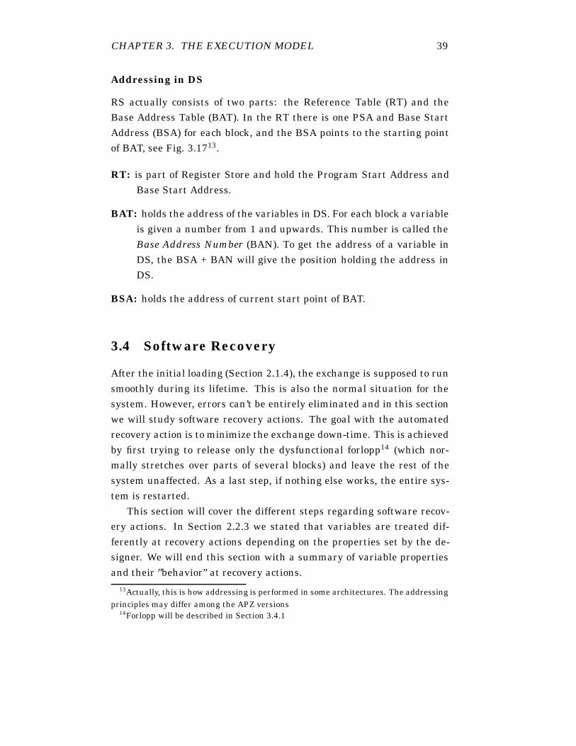
Addressing in DS
RS actually consists of two parts: the Reference Table (RT) and theBase Address Table (BAT). In the RT there is one PSA and Base StartAddress (BSA) for each block, and the BSA points to the starting pointof BAT, see Fig. 3.1713.
RT: is part of Register Store and hold the Program Start Address andBase Start Address.
BAT: holds the address of the variables in DS. For each block a variableis given a number from 1 and upwards. This number is called theBase Address Number (BAN). To get the address of a variable inDS, the BSA + BAN will give the position holding the address inDS.
BSA: holds the address of current start point of BAT.
3.4 Software Recovery
After the initial loading (Section 2.1.4), the exchange is supposed to runsmoothly during its lifetime. This is also the normal situation for thesystem. However, errors can’t be entirely eliminated and in this sectionwe will study software recovery actions. The goal with the automatedrecovery action is to minimize the exchange down-time. This is achievedby first trying to release only the dysfunctional forlopp14 (which nor-mally stretches over parts of several blocks) and leave the rest of thesystem unaffected. As a last step, if nothing else works, the entire sys-tem is restarted.
This section will cover the different steps regarding software recov-ery actions. In Section 2.2.3 we stated that variables are treated dif-ferently at recovery actions depending on the properties set by the de-signer. We will end this section with a summary of variable propertiesand their ”behavior” at recovery actions.
13Actually, this is how addressing is performed in some architectures. The addressingprinciples may differ among the APZ versions
14Forlopp will be described in Section 3.4.1

CHAPTER 3. THE EXECUTION MODEL 40
PSA BSA
Base Address 1(the word-address of a
stored variable)Base Address 2
.....
Base Address n
BaseAddress
Table
ReferenceTable
PS
BN-R RS DS
1
2
3
Block ABlock B
Block n
.....
Block A
Block B.....
Block n
1 = BSA indicates the starting point of base address table for block A located in referencestore. The BSA will give the absolute address.2 = BAN indicates where the BAT word address for the specific variable is found. BAN is arelative address.3 = The word address indicates where the value of the specific variable is stored in DS.
Figure 3.17: Show how addressing to DS is performed in RS. BSA pointsto the starting point of BAT

CHAPTER 3. THE EXECUTION MODEL 41
3.4.1 Forlopp
The first line of defense for maintaining system availability is the For-lopp release. The purpose of a forlopp release is to allow a single processchain, e.g., a call, to be released without adversely affecting any otherprocesses in the system.
Forlopp originates from the Swedish word ”förlopp” meaning ”se-quence of related events”. In the contents of AXE, a typical forloppwill result in a ”path through the system” which generally will be rep-resented by a chain of linked software resources, such as records. InAXE, the word forlopp can be used to denote both the ”sequence of re-lated events” and the resulting ”path through the system”. The forloppmechanism is implemented in the Maintenance Subsystem, MAS, Fig.2.1. Examples of forlopps are an ordinary telephone call or a command.Some concepts associated with forlopps:
• A forlopp identity (FID), stored in a special register, is assigned toeach process (a call or forlopp). All parts participating in the sameforlopp have the same forlopp identity.
• The forlopp manager (FM) stores information concerning the dif-ferent forlopps.
• When a software error is detected, the FM sends release signals tothe blocks involved according to the information stored in FM. Aforlopp release is hereby performed.
• At a forlopp release, a software error dump is performed, whichmeans that the contents of the records participating in the currentforlopp are dumped15.
To summarize, a detected software fault may result in a forlopp release,provided that the function block in which the fault occurred is forlopp-adapted and the forlopp function is active.
3.4.2 System Restart
The system restart has been the traditional recovery action taken by theAPZ (Section 2.1) when it detects a software fault. The system restart
15Section 2.1.4 describes what a dump is.

CHAPTER 3. THE EXECUTION MODEL 42
affects the entire system and not only the forlopp in which the faultoccurred. The purpose of a system restart is to restore the system to apredefined state.
During restart, restart signals are sent to each block, so that duringsuccessive restart phases, blocks perform actions to complete the initial-ization or restoration to a consistent value of their data store variables.
The system restart procedure could be initiated manually, by a COMMAND(Section 2.1.3), or automatically. A manual system restart clears errorsituations, for instance the disconnection of a hanging device. An auto-matic system restart is detected by programs, microprograms and su-pervisory circuits. At a system restart, the job table, the job buffers andthe time queues (Section 3.2) are cleared.
There are three levels of system restart activities:
• Small system restart, which does not affect calls in speech positionand semi-permanent connections. Other calls are disconnected.This is a minimal system restart.
• Large system restart in which all calls are disconnected. Semi-permanent connections are not affected.
• Reload and large system restart in which a reload is performedfirst to ensure that RELOAD-marked variables contain correct val-ues. This is then followed by a large system restart. Semi-permanentconnections are disconnected and automatically reestablished.
The reason to have different types of system restarts is to disturb traffichandling as little as possible during the restart phase.
With the occurrence of the first fault in a normal block that leads toa system restart, the system tries to repair itself without disturbing thetraffic too much - A small system restart is initiated. If another seriousfault occurs within a predefined time interval, a large system restartwill be initiated. In the event of the occurrence of a third serious faultwithin another predefined time interval, a reload and a large systemrestart will take place. This represents the system’s most extreme error-recovery action. The described phases is pictured in Fig. 3.18.
Finally, it is sometimes unnecessary to immediately initiate an auto-matic system restart. The system restart could be delayed or inhibited.This is done by calling the selective restart function.

CHAPTER 3. THE EXECUTION MODEL 43
timex min x min
SmallRestart
SmallRestart
LargeRestart
Reload+
LargeRestart
Figure 3.18: Different types of system restart.
3.4.3 Forlopp Release or a System Restart?
In Section 3.4.1 we described the concept of forlopps as a way to recoverfrom a software error without affecting more than the faulty forlopp.Then, in the following Section, 3.4.2, we described the system restartand the different levels of restart and when they apply. This sectionexplains when the system restart action takes over from the forlopprelease mechanism.
As we said in Section 3.4.1, a forlopp release is always a first choice ifan error has been detected. The system restart ”function” applies whenand if:
• The forlopp release fails to recover the system (i.e., the faulty for-lopp), or
• The faulty process has not been forlopp-adapted, or
• The number of faults have been to high according to a predeter-mined limit.
The last case is checked against an intensity counter. This counter keepstracks of the quantity of software faults. The counter is stepped eachtime a fault is detected leading to a delayed system restart or a forlopprelease. When the counter reaches the predetermined limit, a systemrestart is initiated. The counter is then reset and starts again fromzero. Fig. 3.19 shows the intensity counter and Fig. 3.20 shows thedifferent levels of software recovery.

CHAPTER 3. THE EXECUTION MODEL 44
time
Countervalue
Restart limit (default = 25)
+5
+10
+3
-1 every hour
No restartError is ignored
Delayedrestart
Forlopprelease
Figure 3.19: The intensity counter.
ERROR
Forlopp releasepossible and active?
SelectiveRestart active?
Intensitycounter high?
Check blockcategory
Error ignored
Delayed restart
Immediate restart
Delayed restart with reload
System Restart
0 1 2 3
Yes Forlopprelease
System Restart
No
No
No
Yes
Yes
Figure 3.20: Different levels of recovery after a detected software error.

CHAPTER 3. THE EXECUTION MODEL 45
3.4.4 Variables and Software Recovery
As said in Section 2.2.3, the variable properties determine how the vari-ables are to be treated (i.e., from a data point of view) in the case of asystem restart. Fig. 3.21 shows the principles of how different types ofvariables should be treated after a system restart.
DS DS DUMP DS STATIC DS RELOAD DS RELOAD DUMP DS RELOAD STATIC
DS CLEAR DS CLEAR DUMP
StartSmall
system restartLarge
system restart
System restartwith
reloading Cannot be trusted
Cannot be trusted
Can be trusted Can betrusted
Can be trusted
Cannot be trusted Exception: when the variable value is checked in system restart routine
Figure 3.21: Data security of different start/restart types.

Part II
Semantics

Chapter 4
Related Work
In Section 1.1, we mentioned that efforts have been made to replacePLEX with, or ”map” PLEX to, specification languages like SDL for in-stance. The latest version of SDL (Specification and Description Lan-guage), SDL2000, has been given a formal (semantic) definition1. Workon this can be found in [IT00] and [EGG+01]. Whether or not SDLand PLEX are ”compatible” with each other is still discussed within thePLEX design group, and will not be a subject of study in this report.
Another language used for specification is UML, Unified ModelingLanguage. The relation between PLEX and UML has been discussedin [AGG99]. A dialect of UML, UML-RT, is discussed by Herzberg in[Her99]. This paper investigates the mapping between PLEX and UML-RT. This paper is published within the E-CARES project2, which alsoexplores the AXE system, but from a ”re-engineering” point of view.
Another language used in the same domain, i.e., the telecommuni-cation domain, is CHILL (CCITT High Level Language), which was de-veloped by the International Telecommunication Union (ITU), [IT99].The language has been specified by the Vienna Development Method,[BJ82], in [IT82]. This is a denotational framework and could be of in-terest since CHILL is used in the same domain as PLEX. But, since theVDM is more of a specification method, that goes from abstract notation
1See the home page of the SDL Formal Semantics Project on:http://rn.informatik.uni-kl.de/projects/sdl/
2Home page:http://www-i3.informatik.rwth-aachen.de/research/projects/ecares/Main.html

CHAPTER 4. RELATED WORK 48
to formal specification, whereas this work goes from an implementedlanguage to a formal specification, the VDM will not be considered inthis report.
CHILL has also been covered by Winkler in [Win00].

Chapter 5
Programming LanguageSemantics
What is programming language semantics and how/when is it used?The first section in this chapter is devoted to answer these questions.We will explain what we mean by a semantic description of a program-ming language. The following sections will look at the most commonforms of semantics.
5.1 The meaning of a program
Programming language semantics is concerned with rigorously speci-fying the meaning, or the effect, of programs that are to be executed.By effect we mean, for instance, the contents of the memory locations,which parts of the program that is to be executed, or the behavior of thehardware affected by the program. A semantic specification capturesthese things in a formal way, and later in this chapter we will studydifferent approaches to this formal description.
Formal descriptions of programming languages are becoming moreand more popular, e.g. the BNF1 is used to specify the syntax of PLEX.The problem is that a formal description of the syntax says nothingabout the meaning of the program since ”syntax is concerned with thegrammatical structure of programs” whereas ”semantics is concerned
1Backus-Naur Form

CHAPTER 5. PROGRAMMING LANGUAGE SEMANTICS 50
with the meaning of grammatically correct programs” [NN92]. It is alsopossible to distinguish between static and dynamic semantics [Mos01].Static semantics corresponds to the compile-time behavior of the pro-gram, the dynamic semantics hence corresponds to the run-time behav-ior.
But now when we know what programming language semantics is,how can we use it? We consult [NN92] for an answer to this question:
• The semantics can reveal ambiguities and complexities in whatmay look as a clear documentation of the language (e.g. the lan-guage manual).
• The semantics can also form the basis for implementation, analy-sis and verification.
Even with these obvious advantages with formal semantics, it is stillwidely regarded as being of interest only to theoreticians [Mos01].
5.2 Semantic approaches
The formalizations of a programming language may differ, i.e. the ex-planations (or the meaning) can be formalized in different ways. Mostframeworks, or approaches, can be classified as one of the followingthree categories:
• Operational semantics - How to execute the program. The opera-tional approach(es) is (are) concerned with how the effect of thecomputations is produced. The meaning is often specified by anabstract machine and/or a transition system.
• Denotational semantics - The effect of executing the program. De-notational semantics, in contrast to operational semantics, is onlyconcerned with the effect of the computation, not how it is ob-tained. Meanings are modeled by mathematical objects represent-ing the effect of executing the constructs.
• Axiomatic semantics - Partial correctness properties of the program.The axiomatic approach is concentrated on specific properties of a

CHAPTER 5. PROGRAMMING LANGUAGE SEMANTICS 51
program. These properties are expressed as assertions. Axiomaticsemantics involves rules for checking these assertions. There maybe aspects of the executions that are ignored since only specificproperties are considered.
These different categories will be further investigated/explained in theirown sections (5.4, 5.5 and 5.6), but we can already state that in thegeneral case, the semantics will tell us something about the relationbetween an initial and a final state2.
5.3 Notation
In the following studies of the different approaches, some ”semantic”notations will be used3. These notations may seem unfamiliar to thereader and we will summarize some basic notations here.
• By [x �→ 5] we mean the function that maps the symbol x to thenumerical value 5. I.e. x has the value 5.
• s0 = [x �→ 5] is called a state. The state s0 where x maps to 5. Wewill also use the general form s x to denote the variable x in states. For a value 3, bound to x in the state s, we will write s x = 3.
• By 〈x := z, s0〉 → s1 we mean that the execution of x:=z in the states0 will result in the new state s1.
• We will later talk about semantic functions and use the notation [[ ]]to denote the syntactic argument (enclosed in syntactic brackets)to the semantic function.
• We will use tt and ff to denote the truth values true and false,respectively.
• 〈 S1, s 〉 → s′, 〈 S2, s′ 〉 → s′′〈 S1; S2, s〉 → s′′ is called a rule. It has a number of
premises above the solid line and one conclusion below the solidline. A rule may also have a number of conditions that have to befulfilled whenever the rule is applied.
2The meaning of a state is explained in the following subsection.3The notation used in this report are the same as used in [NN92]

CHAPTER 5. PROGRAMMING LANGUAGE SEMANTICS 52
• We will use ⇒ as the transition relation, i.e., when we go from onestate to another with the execution of one statement.
• ⇒∗ means that we take zero or more steps from an initial to a finalstate.
5.4 Operational Semantics
In Section 5.2 we said that a semantic formalism tells us somethingabout the relationship between the initial and the final state. In theOperational approach we are not only interested in this relationship.We also want to know how the computations that lead to the final statemodify the intermediate state(s) as well. The different operational ap-proaches differ in the level of details:
• In the Natural semantics, the focus is on how the overall results ofthe executions are obtained, whereas
• in the Structural operational semantics, it is of interest in how theindividual steps of the execution takes place4.
These two different approaches will be studied in the following subsec-tions (5.4.1 and 5.4.2). For both styles of operational semantics, themeaning of statements is specified by a transition system with two dif-ferent configurations:
• 〈S, s〉 which means that the statement S is to be executed from thestate s.
• s that represent a terminal state, i.e. a termination of the compu-tation.
5.4.1 Natural Semantics
The relationship between the initial and the final state of the executionof a statement is in focus for the natural semantics (ns). The transitionsystem specifies this relationship for every statement and is written in
4Natural semantics is also known as Big Steps Semantics, whereas the structuraloperational approach sometimes is called Small Steps Semantics. These alternativenames tell us something about how detailed the transition is specified.
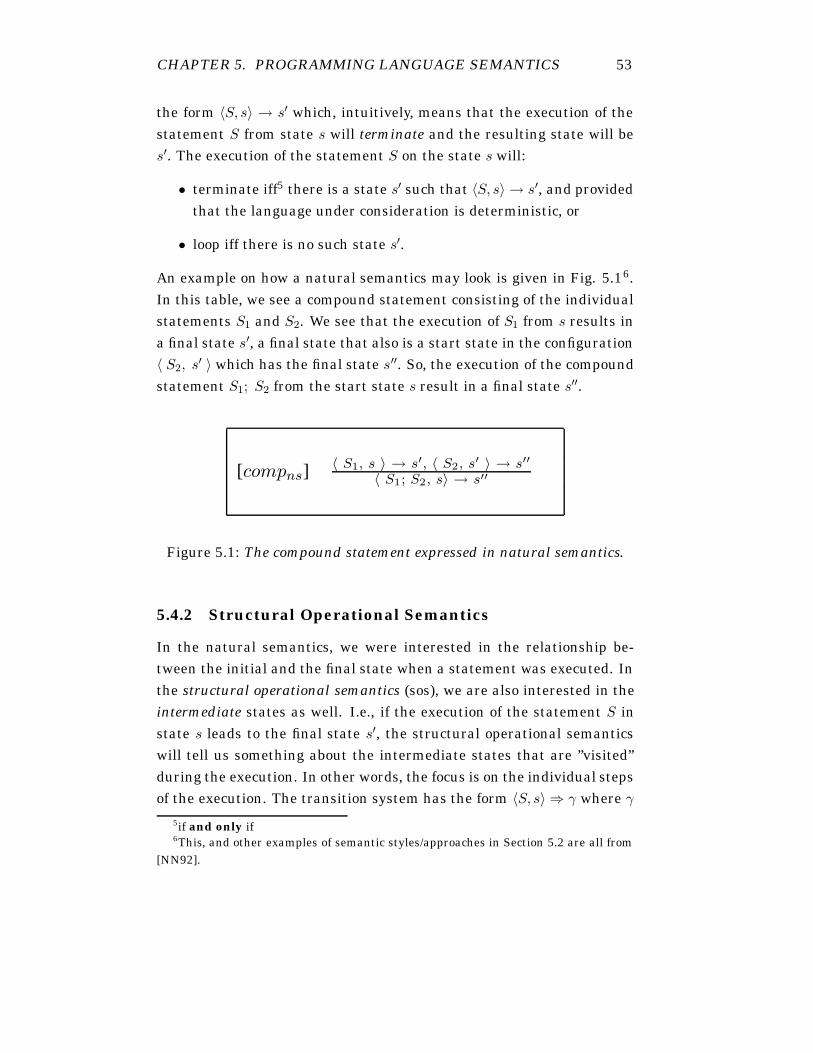
CHAPTER 5. PROGRAMMING LANGUAGE SEMANTICS 53
the form 〈S, s〉 → s′ which, intuitively, means that the execution of thestatement S from state s will terminate and the resulting state will bes′. The execution of the statement S on the state s will:
• terminate iff5 there is a state s′ such that 〈S, s〉 → s′, and providedthat the language under consideration is deterministic, or
• loop iff there is no such state s′.
An example on how a natural semantics may look is given in Fig. 5.16.In this table, we see a compound statement consisting of the individualstatements S1 and S2. We see that the execution of S1 from s results ina final state s′, a final state that also is a start state in the configuration〈 S2, s′ 〉 which has the final state s′′. So, the execution of the compoundstatement S1; S2 from the start state s result in a final state s′′.
[compns]〈 S1, s 〉 → s′, 〈 S2, s′ 〉 → s′′
〈 S1; S2, s〉 → s′′
Figure 5.1: The compound statement expressed in natural semantics.
5.4.2 Structural Operational Semantics
In the natural semantics, we were interested in the relationship be-tween the initial and the final state when a statement was executed. Inthe structural operational semantics (sos), we are also interested in theintermediate states as well. I.e., if the execution of the statement S instate s leads to the final state s′, the structural operational semanticswill tell us something about the intermediate states that are ”visited”during the execution. In other words, the focus is on the individual stepsof the execution. The transition system has the form 〈S, s〉 ⇒ γ where γ
5if and only if6This, and other examples of semantic styles/approaches in Section 5.2 are all from
[NN92].

CHAPTER 5. PROGRAMMING LANGUAGE SEMANTICS 54
is either of the form 〈S′, s′〉 or of the form s′. This means that the tran-sition system expresses the first step of the execution of the statementS from the state s and the result of this is γ.
• If γ is of the form 〈S′, s′〉 then the execution of S from s is notcompleted and the rest of the computation is expressed by the in-termediate configuration 〈S′, s′〉.
• If γ, on the other hand, is of the form s′, then the execution of S
has terminated and the final state is s′.
In Fig. 5.2 we express the compound statement in a structural opera-tional semantics style. Unlike the natural semantics in Fig. 5.1, we seetwo ”cases” for the compound statement. In the first case, the executionis not completed and the next configuration (from 〈S1, s〉) is the inter-mediate configuration 〈S′
1, s′〉. In the second case, the execution of S1 is
completed and the final state is s′. From this state, the execution of theconfiguration 〈S2, s
′〉 can start.
[comp 1sos]
〈 S1, s〉 ⇒ 〈 S′1, s′ 〉
〈 S1; S2, s 〉 ⇒ 〈 S′1; S2, s′ 〉
[comp 2sos]
〈 S1, s〉 ⇒ s′〈 S1; S2, s 〉 ⇒ 〈 S2, s′ 〉
Figure 5.2: The compound statement expressed in structural operationalsemantics.
5.5 Denotational Semantics
With the operational approach, the focus was on how the program wasexecuted - ”How to compute.” In the denotational approach, the empha-sis is on ”the effect of computing”. By effect, we mean the relationshipbetween the initial and the final state. The denotational approach con-sists of defining semantic functions for each syntactic category. This

CHAPTER 5. PROGRAMMING LANGUAGE SEMANTICS 55
semantic function maps each syntactic construct to a mathematical ob-ject, most often a function, that describes the effect of executing the con-struct. In Fig. 5.3, we see a denotational description of the compoundstatement (previously shown in Figure 5.1 and 5.2). In the Figure, wesee that the effect of computing the compound statement S1; S2 is thefunctional composition of executing S1 followed by S2.
Sds[[S1; S2]] = Sds[[S2]] ◦ Sds[[S1]]
Figure 5.3: The compound statement expressed in denotational seman-tics.
5.6 Axiomatic Semantics
With the operational as well as the denotational approach, we are con-cerned with the meaning of a given program. This is in contrast tothe axiomatic approach were we study properties of a given program.These properties (expressed as assertions) could, for instance, be exe-cution times (see [NN92] for an example) or the degree of resource uti-lization. But, since the focus is on specific properties and not on themeaning (as in the previously described styles) ”there may be aspects ofthe execution that are ignored” [NN92]. Axiomatic definitions is oftengiven in the form
{P}S{Q}
where P is a Pre-condition, S the statement to be executed and Q a Post-condition. This is to be interpreted as: ”If P holds and the execution ofS terminates, then Q will hold”. In Fig. 5.4 we show the compoundstatement in the axiomatic style. From this, we can say that if the pre-condition P holds and the execution of S1 followed by the execution of S2
terminates holds, then the post-condition R will hold.
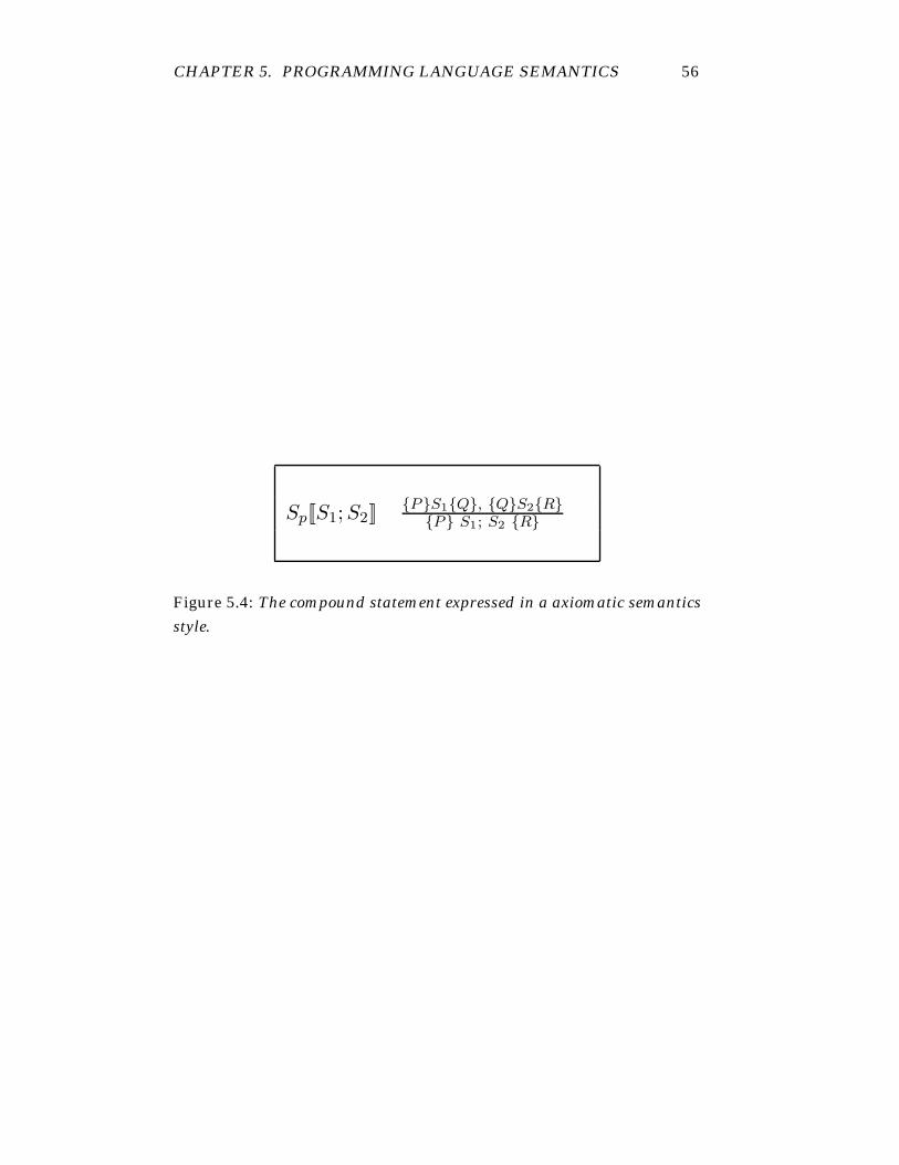
CHAPTER 5. PROGRAMMING LANGUAGE SEMANTICS 56
Sp[[S1;S2]]{P}S1{Q}, {Q}S2{R}
{P} S1; S2 {R}
Figure 5.4: The compound statement expressed in a axiomatic semanticsstyle.

Chapter 6
Semantic Approach
6.1 Selected Approach and Motivation
In the process to determine a proper semantic approach for PLEX, itwas early agreed that the axiomatic approach (described in Section 5.6)was not a suitable choice because of the rather abstract notation andalso because its focus is on properties more than the effect. So, theselection had to be made between some form of operational semantics,or the denotational approach. Some considerations that were taken intoaccount:
• The operational semantics has its main advantages1 in the factthat it is relatively easy to understand and also that the execu-tional steps are explicit. A possible disadvantage may be the factthat the approach is tightly connected to how a statement is exe-cuted (i.e., it is closer to the actual execution than the denotationalapproach).
• For the denotational approach, the advantage is that since mathe-matical objects are in focus, it abstracts away from how programsare executed. It can therefore be seen as the denotational ap-proach provides a more formal basis for reasoning about programs.The disadvantage lays in the notation - Mathematical notationmay ”scare” the unfamiliar reader.
1This is the authors opinion.

CHAPTER 6. SEMANTIC APPROACH 58
[NN92] claims that the denotational approach may be preferred whenreasoning about programs whereas the operational approach may bepreferred when implementing the language. The decision to use an op-erational approach was based on the following considerations:
• It was a pre-request that the notation would be relatively easy tounderstand even by a reader unfamiliar with semantic notation.
• The language PLEX is continuously updated and new hardware isintroduced in periodic intervals. This means that our semantic de-scription also could be seen as a reference manual for new (future)implementations of the language.
A second decision had to be made whether we should use the nat-ural semantics (described in Section 5.4.1) or the structural operationalsemantics (described in Section 5.4.2). Even if the PLEX language doesnot provide parallelism today, it is shown that many constructs are suit-able for parallel execution [Lin03], and to be able to deal with this in afuture extension of the (language and the) semantics, the structural op-erational approach were preferred2.
6.2 The State of the System
In order to develop a semantic framework for PLEX, we have to deter-mine what a state of the system is since the execution of a statement willchange the current state, i.e., with the execution of a statement, we gofrom an old state to a new state. Our starting point will be:
• With the state of the system, we mean the contents of the memory.
So, in order to determine the state of the system, we will look at thedifferent forms of storage that exist in the system.
The first thing we have to consider is the memory and stores of theCentral Processor. The memory in the Central Processor (CP) consistsof the register memory and the different stores.
2[NN92] shows why the structural operational semantics is well suited for parallelconstructs.

CHAPTER 6. SEMANTIC APPROACH 59
The register memory is used for storing of temporary variables, point-ers and for transferring of signal data between different ”processes”3.Values in the registers are lost after an EXIT from a job, or other reg-ister killing statements such as direct signals, combined signals or IOstatements, for example. These are all statements that force the exe-cution to leave the current block. Temporary variables are only ”alive”(i.e., containing a value in a register) from the first write to it, until thelast use. The PLEX compiler keeps track of write-read chains and onlyallocates registers while the variables are alive during the execution.
The different stores in the CP were shown in Fig. 2.2. They are re-peated in Fig. 6.1. The different forms of storage contains the followinginformation:
• The Program Store is used for the storage of programs.
• Variables that is to survive the termination of a ”process” or a sys-tem restart, are stored in the Data Store.
• The Reference Store, finally, contains information about where tofind the different programs and data.
However, the Program Store and the Reference Store will be omittedwhen we specify the state of the system since the statements we look at(starting in Section 6.12) don’t effect these storages. The second thing
Program Store
PS
Reference Store
RS
Data Store
DS
Figure 6.1: The different stores in the central processor (CP).
that is important, is the different kind of job buffers (which are used tostore the different kinds of signals). A simplified figure of the job buffersis shown in Fig. 6.24. The semantics of the job buffers are the FIFO5
3The transferring of signal data have similarities to an ordinary function call: Justas variables are loaded when the function is entered, are the signal data loaded at thestart of a sub-program, i.e., at a SIGNAL ENTRY.
4A more detailed description is found in Fig. 3.10.

CHAPTER 6. SEMANTIC APPROACH 60
JBA - urgent tasks of the operating system; preferential traffic JBB - all other telephone traffic JBC - input/output to operator and I/O devices JBD - APZ routine self-tests JBR - Signals from Central Processor to Regional Processor
Job buffers for CP-CPand RP-CP signals
Job buffer for CP-RP signals
JBA
JBB
JBC
JBD
JBR
Figure 6.2: A simplified figure of the job buffers in the PLEX/AXE envi-ronment. (See also Fig. 3.10)
approach, as shown in Fig. 6.3. Associated with each job buffer aretwo pointers, Job Buffer In (JBI) and Job Buffer Out (JBO). Thesepointers make it possible for the APZ (the operating system) to knowwhere, in a job buffer, to insert a signal that is to be buffered, or fromwhere to fetch a new signal. The memory layout, in a job buffer, for onebuffered signal is pictured in Fig. 6.4. The job buffer will consequentlyconsist of several items of the form described in the picture. So, as
...Enter SigA
...
Unit B
Job Buffer...Send SigA
...EXIT
...
Unit A
JBI JBO
Figure 6.3: The FIFO-semantics of the job buffers.
stated in the beginning of this section, our starting point in determiningthe state of the system, was:
• With the state of the system, we mean the contents of the memory.5First-In-First-Out

CHAPTER 6. SEMANTIC APPROACH 61
W0
W1
W2
W3
W4
W5
W6
W7
W8
W9
W10
W11
Wn
IPOINTER LI
0 BN|R
0 BN|S
BN|S ND
FORLOPP ID B0 15
STYPE 0L F
FORLOPP ID B16 31TR
POINTER B0 15
POINTER B16 27
DATAWORD 0
DATAWORD 1
DATAWORD N
0 LSN (SNX)
LI - Lengt Indicator LSN - Local Signal Number. The entry point in the Signal Distribution Table of the receiving block DATAWORD <p> - Where the actual data is placed
Figure 6.4: Organization of the job buffers. NOTE: The pointer registers,W8-W9, are treated as one register (and referred to as POINTER B0).This is due to the fact that the register in W9 is only used when a pointeris too large to fit only in W8. In this case, the pointer will be split up andplaced in W8 with its first half, and in W9 with its second half.

CHAPTER 6. SEMANTIC APPROACH 62
And, we can now tell that the contents of the memory is the contents ofthe register memory, the contents of the Data Store, and the contents ofthe job buffers. The state of the system can, at this point, be representedas a tuple of the form6:
〈RM,DS, JBA, JBB, JBC, JBD, JBR〉
where RM = Register Memory, DS = Data Store, JBA = Job Buffer A,JBB = Job Buffer B, JBC = Job Buffer C, JBD = Job Buffer D and JBR= Job Buffer R.
The above representation would indeed be sufficient if PLEX was astrictly sequential language, i.e., if statementA precedes statementB inour source code file, then we could be absolutely certain that statementA
would execute before statementB. This holds in a language without thepossibility to manipulate the Program Counter, e.g., with a JUMP state-ment. But since these kind of statements do exist in PLEX7, we alsohave to model the possibility of ”moving” the execution to somewheredifferent from the following statement. If we had been dealing withsome kind of assembler code, the above could easily be managed by ad-justing the Program Counter according to the instructions executed bythe CPU. But we are not looking at the semantics from an instructionlevel point of view, instead we are working with statements that consistsof n instructions.
• Our solution is to define the Virtual Statement Counter, VSC
The VSC contains an address (an integer value), which tells where thefirst instruction in the next statement resides in memory. By steppingup the VSC with 1, we step it up to the first instruction in the nextstatement8. If nothing else is stated, the VSC will always be stepped upto the next statement after the execution of a previous statement, i.e.,s[VSC �→ VSC+1]. For convenience, we will use the notation s[VSC++]
6The contents of the memory could also be extended with the contents of the DATA
SECTOR (see Section 2.2.1), which is used in a startup phase as well as in a systemrestart phase. But since we do not cover those phases in this report, the contents of theData Sector is omitted in our description of the systems state.
7E.g., the GOTO statement.8The approach is similar to the one described in [Lis98], where the program counter
is modified in a similar way.

CHAPTER 6. SEMANTIC APPROACH 63
to denote s[VSC �→ VSC+1]. In situations where this is obvious, we willomit this ”information”. A situation where this is the case would forinstance look like: 〈S1, s〉 ⇒ 〈S′
, s′〉
The above leads us to the following definition of the state of the sys-tem:
〈VSC, RM,DS, JBA, JBB, JBC, JBD, JBR〉
6.3 Lexical Units and Syntactical Categories
In this section9, we will follow the conventions in [AB02] and use thesame variant of EBNF (Extended Backus-Naur Form) notation.
• ::= is used as the ”definition operator”.
• We will mark a KEYWORD with bold, upper case letters.
• The vertical bar, |, represents a choice between elements.
• The square brackets [ ] are used to denote an optional construct.I.e., the construct inside the brackets may be omitted.
• Optional properties are marked in a separate way, like in ”length”.
• Curly brackets, { }, are used to delimit an operand, or simply toimprove readability. { }∗ represents a possibly empty sequence ofelements, i.e., the element may be repeated zero or more times.Finally, { }+, are used for the non-empty sequence of elements.
The lexical units and the syntactic categories10 in PLEX are as follows:
• upper-case-letter ::= A|B|C|...|X|Y|Z
• lower-case-letter ::= a|b|c|...|x|y|z
• letter ::= upper-case-letter | lower-case-letter• decimal-digit ::= 1|2|3|...|7|8|9
• hexadecimal-digit ::= 1|2|...|8|9|A|B|...|E|F
• special-character ::= !|"|#|%|1|’|?|(|)|*|+|,|-|.|/|:|;|<|=|>|_
|[|]|$|@
9The syntactical material in this section is basically compiled together from thefollowing internal Ericsson documents: [AB98, AB02, AB86]
10Please note that the syntactical categories in this section are only a subset of thelanguage.
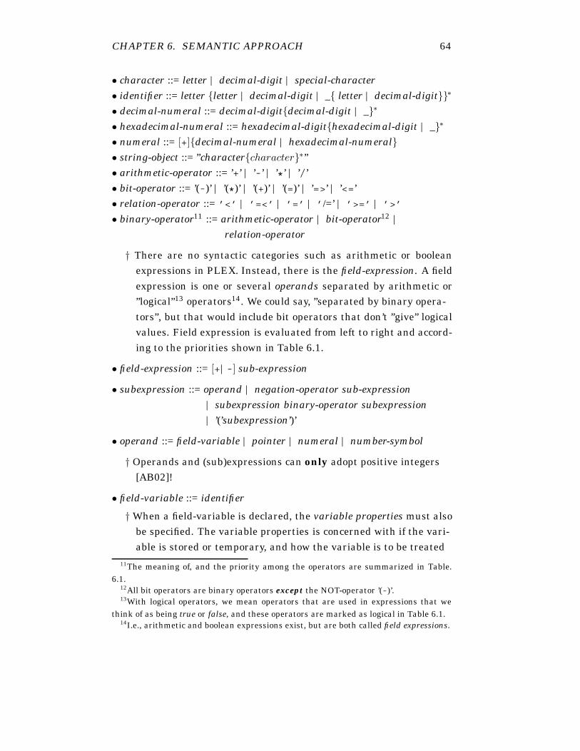
CHAPTER 6. SEMANTIC APPROACH 64
• character ::= letter | decimal-digit | special-character• identifier ::= letter {letter | decimal-digit | _{ letter | decimal-digit}}∗
• decimal-numeral ::= decimal-digit{decimal-digit | _}∗
• hexadecimal-numeral ::= hexadecimal-digit{hexadecimal-digit | _}∗
• numeral ::= [+]{decimal-numeral | hexadecimal-numeral}• string-object ::= ”character{character}∗”• arithmetic-operator ::= ’+’ | ’-’ | ’*’ | ’/’• bit-operator ::= ’(-)’ | ’(*)’ | ’(+)’ | ’(=)’ | ’=>’ | ’<=’• relation-operator ::= ’<’ | ’=<’ | ’=’ | ’/=’ | ’>=’ | ’>’
• binary-operator11 ::= arithmetic-operator | bit-operator12 |relation-operator
† There are no syntactic categories such as arithmetic or booleanexpressions in PLEX. Instead, there is the field-expression. A fieldexpression is one or several operands separated by arithmetic or”logical”13 operators14. We could say, ”separated by binary opera-tors”, but that would include bit operators that don’t ”give” logicalvalues. Field expression is evaluated from left to right and accord-ing to the priorities shown in Table 6.1.
• field-expression ::= [+|-] sub-expression
• subexpression ::= operand | negation-operator sub-expression| subexpression binary-operator subexpression| ’(’subexpression’)’
• operand ::= field-variable | pointer | numeral | number-symbol
† Operands and (sub)expressions can only adopt positive integers[AB02]!
• field-variable ::= identifier
† When a field-variable is declared, the variable properties must alsobe specified. The variable properties is concerned with if the vari-able is stored or temporary, and how the variable is to be treated
11The meaning of, and the priority among the operators are summarized in Table.6.1.
12All bit operators are binary operators except the NOT-operator ’(-)’.13With logical operators, we mean operators that are used in expressions that we
think of as being true or false, and these operators are marked as logical in Table 6.1.14I.e., arithmetic and boolean expressions exist, but are both called field expressions.

CHAPTER 6. SEMANTIC APPROACH 65
during software recovery actions. The property is specified as avalid15 combination of the keywords: DS, BUFFER, COMMUNI-CATION BUFFER, CLEAR, SEMICLEAR, RELOAD, DUMP,STATIC and TRANSIENT
• pointer ::= POINTER pointer-name ’(’record-name’)’ ’;’
• pointer-name ::= identifier• record-name ::= identifier
† [AB98] states that the pointer-name should end with the suffixpointer, ptr or p.
†† Pointers are not more than record numbers (i.e., positive integers).A pointer is always associated with a file and the value of thepointer is the number of the current record in that file. (See Sec-tion 2.2.2 for details.)
††† Pointers behave like, and are treated as, temporary variables,i.e., pointers are stored in the register memory and they may loosetheir value whenever the execution of the software unit termi-nates.There is no explicit pointer arithmetic, instead they are treatedand used as operands in field-expressions (described above) and inassignment statements (described later in this section).
• number-symbol ::= identifier† Number symbols have the same semantic meaning as constants inC (for example).
†† Number symbols are declared in the Declare Sector (see Section2.2.1) with the statement:NSYMB identifier ’=’ {decimal-numeral | hexadecimal-numeral}’;’
• condition ::= field-expression relation-operator field-expression| symbol-variable [’=’ | ’/=’] symbol-value| string-object [’=’ | ’/=’] string-object
• symbol-variable ::= SYMBOL VARIABLE’(’symbol-value {, symbol-value}∗’)’ [properties] ’;’
• symbol-value ::= identifier
• properties= A valid combination of: DS, BUFFER, COMMUNI-15The valid combinations of the variable properties, as well as the meaning of the
different properties is covered in Section 2.2.3.

CHAPTER 6. SEMANTIC APPROACH 66
CATION BUFFER, CLEAR, SEMICLEAR, RELOAD, DUMP,STATIC and TRANSIENT
† Symbol variables are also known as enumeration type variables, aconcept that is familiar to C programmers. Their use is to holdsymbol values, which in the AXE domain could be IDLE, BUSY,BLOCKED for instance. A symbol variables can be assigned symbolvalues and compared to other symbol variables.
†† The code generation phase16 replaces the symbol values with nu-merical values. This is why symbol variables can be assigned to,and compared with, field variables (that store numerical values),i.e., if a field variable is assigned a symbol value, the numericalvalue of the symbol is assigned the field variable.
Priority Operator Meaning Type1 (-) Logical NOT Bit operator (logical)2 => Shift right Bit operator2 <= Shift left Bit operator3 * Multiplication Arithmetic3 / Division Arithmetic4 +, - Addition, Subtraction Arithmetic5 = Equality Relation (logical)5 /= Inequality Relation (logical)5 < Less than Relation (logical)5 > Greater than Relation (logical)5 =< Less or equal than Relation (logical)5 >= Equal or greater than Relation (logical)6 (*) Logical AND Bit operator (logical)7 (=) Logical XOR (Exclusive or) Bit operator (logical)8 (+) Logical OR Bit operator (logical)
Table 6.1: Priorities and meaning of the PLEX operators. Priorities arenumbered from the highest (1) to the lowest (8).
16The code generation phase is the process of translating (in several steps) the sourcecode (PLEX) to machine code. (The compilation process, in which the code generationtakes place, is covered in [AE00].)

CHAPTER 6. SEMANTIC APPROACH 67
6.4 Statements for Variable Assignments
The general form of the assignment statement has the following syntax:
• assignment-statement ::= [SET] variable ’=’ expression ’;’
We recall (from Section 2.2.3) that PLEX have three different types ofvariables; Field variables for numerical information, symbol variablesfor symbolic values, e.g., IDLE, BLOCKED, BUSY, etc and string vari-ables which store text strings. This implies the following three state-ments for variable assignment:
• field-assignment-statement ::= [SET]{ { {pointer | field-variable} ’=’ }+
{field-expression | maxnum-expression} }| { field-variable ’=’}+ symbol-variable ’;’
• maxnum-expression ::= MAXNUM OF variable
† The value of a maxnum-expression is the number of individuals inthe file associated with the given variable name.
• symbol-assignment-statement ::=[SET] {symbol-variable ’=’}+ symbol-value ’;’
• string-assignment-statement ::=[SET] {string-variable ’=’}+ string-object ’;’
6.5 Jump Statements
PLEX offers both conditional and unconditional jump statements. The”programmer guidelines” for the use of jump statements are: ”Pleaseavoid backward jumps as far as possible, because they are difficult tofollow.” and ”Try to avoid jump statements, since they can give rise toa poor program structure. It is very difficult to read a program with agreat many jump statements.” [AB98]. But still, they are part of thelanguage, and we will look at their syntax here.
The unconditional jump statement simply interrupts the sequentialexecution order and its syntax is as follows:

CHAPTER 6. SEMANTIC APPROACH 68
• unconditional-jump-statement ::= {GOTO | GO TO} label ’;’
The conditional jump statement offers a possibility to jump if the givencondition is met. It has the form of an if-statement with a goto:
• if-statement ::= IF [NOT] condition [PROCEED ELSE]{GOTO | GO TO} label ’;’
Since condition will return in other statements, its syntax is given here:
• condition ::= {field-expression1 relation-operator field-expression2}| {symbol-variable {’=’ | ’/=’} symbol-value}| {string-object {’=’ | ’/=’} string-object }
In connection to the jump statements, there is also the BRANCH state-ment which selects between a number of program sequences, but sincethis statement has been ”removed”17 from the language, we will notcover it here.
6.6 Conditional Statements
The if-statement in Section 6.5 is a rather primitive construction sinceit does not have an else clause and because the only permitted actionis an unconditional jump. This is the motivation for the following morerecent statement:
• improved-if-statement ::=IF [NOT] condition THEN sequence-of-statements
{ELSEIF [NOT] condition THEN sequence-of-statements}∗
[ELSE sequence-of-statements]FI
17I.e., it is an old statement and should be avoided in new design [AB98].

CHAPTER 6. SEMANTIC APPROACH 69
6.7 Selections
The CASE statement is used for selection between an arbitrary18 num-ber of unambiguous choices:
• case-statement ::=CASE expression IS
{WHEN choice {’,’ choice}∗ DO sequence-of-statements}+
OTHERWISE DO sequence-of-statementsESAC ’;’
• expression ::= field-expression | symbol-variable | string-object
• choice ::= numeral | number-symbol | symbol-value | string-symbol| text-string
It is not allowed to use a signal reception statement (Section 6.9) insidethe sequence of statements part19. Neither is it allowed to jump into aCASE statement.
6.8 Iterations
The well known While statement is missing in PLEX. The main reasonis that such a construct is not considered necessary in the applicationdomain (which is the central part of the AXE switching system). A sec-ond reason is that the construct may give rise to unpredictable executiontimes, which is not the case with the iteration statements in PLEX (seebelow).
Instead, PLEX offers three different statements for iteration: ON,FOR ALL and FOR FIRST. They are all used for scanning files or in-dexed variables between given start and stop values. The three it-eration statements are compared in Fig. 6.5 and their syntax are asfollows:
• on-statement ::=ON {pointer | field-variable} FROM field-expression
{UPTO | DOWNTO} field-expression
18I.e., one or more19Which also holds for iterations and conditionals.

CHAPTER 6. SEMANTIC APPROACH 70
DO sequence-of-statementsNO ’;’
• for-statement ::=FOR {FIRST | ALL} {pointer | field-variable}
FROM field-expression-1 [UNTIL field-expression-2][WHERE { [NOT] condition
| field-variable IS CHANGED TO field-expression}]{ {GOTO | GO TO} label| DO {statement | statement-block-name} } ’;’
Criterion ON FOR ALL FOR FIRSTAscending or descending order Yes Always descending
Several statements in actionpart
Yes No, except in state-ment blocks, IF, CASEand loop statements
Condition in iteration state-ments
NO Possible Always
Iteration ends after matchingcondition once and handlingone individual
Not applica-ble
No Yes
Iteration variable/pointer afterloop
Undefined Undefined Defined ifmatchingindivid-ual/condition
Generates high-speed loop No20 Possible Possible
Figure 6.5: PLEX iteration statements - a comparison.
6.9 Signal Sending/Receiving Statements
In Section 3.1 it was stated that the main distinction to be made be-tween the different kinds of signals in PLEX is between direct andbuffered signals. And this is true from the point of view of the execu-tion model, but from a syntactical point of view, the main distinctionis between single and combined signals. Every signal will fall into one

CHAPTER 6. SEMANTIC APPROACH 71
of these categories. I.e., from the syntactical point of view it is only ofinterest whether one has to wait for an ”answer” (a combined signal) ornot - Whether the signal is direct or buffered, or unique or multiple,21
is specified in the Signal Description, described in appendix B, and iscertainly of interest from a semantic point of view.
6.9.1 Statements for Single Signals
There are two statements that are concerned with single signals - Thefirst one given is the statement for sending a single signal, whereas thesecond receives a single signal:
• single-signal-transmission-statement ::=SEND signal [REFERENCE field-variable]
[WITH signal-datum {’,’ signal-datum}∗][ [’,’] { BUFFER
| HURRY| DELAY {numeral
| field-variable| field-expression}{MS | S | M}
| DELAY UNTIL {numeral | field-variable}} ]’;’
NOTE: The reference ”variable” must be given if the signal is a multiplesignal, which is stated in the Signal Description. The ”WITH signal-datum” part is the data that the signal is carrying. Current program-ming guidelines says that the keyword BUFFER, which states that thesignal is to be buffered, should not be used in new design [AB98]. Theremaining keywords is concerned with if the signal is to be bufferedor not (HURRY), and if it is to be buffered, for how long (DELAY. . . ).However, if the signal is to be buffered or not, also depends on the in-formation given in the Signal Description, and this will be covered inmore detail in Appendix B.
• single-signal-reception-statement ::=ENTER signal [WITH signal-datum { ’,’
signal-datum}∗ ]’;’20Except for BUFFER CLEAR/COPY (Section 2.2.3).21The different signal types is described in Section 3.1

CHAPTER 6. SEMANTIC APPROACH 72
NOTE: When a signal is fetched from a job buffer, this statement nor-mally marks the entry point in the corresponding code that is to beexecuted22.
6.9.2 Statements for Combined Signals
• combined-forward-signal-transmission-statement ::=SEND cfsignal [REFERENCE field-variable]
[WITH signal-datum {’,’ signal-datum}∗][’,’]WAIT FOR cbsignal1 IN label
{OR cbsignaln IN label}∗ ’;’NOTE: As could be seen in the syntax for the sending of a combinedforward signal, it must be specified where (in the code) the ”answer” issupposed to arrive. Also, note that it is allowed to wait for more than onebackward signal. This is useful when one wants to take action accord-ing to the result of the execution in the block that received the forwardsignal (and then sent the backward signal).The following statement is used for receiving of a forward signal.
• combined-forward-signal-reception-statement ::=RECEIVE cfsignal
[WITH signal-datum {’,’ signal-datum }∗] ’;’
The following two statements is concerned with the answer to the ini-tiating part. The first statement is sending the ”reply” whereas thesecond receives the ”answer”.
• combined-backward-signal-transmission-statement ::=RETURN cbsignal
[WITH signal-datum {’,’ signal-datum}∗] ’;’
• combined-backward-signal-reception-statement ::=label’)’ RETRIEVE cbsignal
[WITH signal-datum {’,’ signal-datum}∗] ’;’
22The entry point for code execution could also be the statement for receiving a com-bined (forward) signal (described in Section 6.9.2).

CHAPTER 6. SEMANTIC APPROACH 73
6.9.3 Statements for Local Signals
The following statements is for the sending, and receiving of a local sig-nal, respectively. (Local signals are described in Section 3.1.4.)
• local-signal-sending-statement ::=TRANSFER signal
[WITH signal-datum {’,’ signal-datum}∗] ’;’
• local-signal-receiving-statement ::=ENTRANCE signal
[WITH signal-datum {’,’ signal-datum}∗] ’;’
6.10 Exit
The exit statement is a deactivation statement for the sequence of state-ments that begins with a signal reception statement for a single signalor a command reception statement.
• exit-statement ::= EXIT ’;’
NOTE: The exit statement marks the (possible) termination of a subpro-gram and also the termination of a job, since the control is transferredback to the operating system (which fetches the next job from the jobbuffers).
6.11 Semantic Functions
In order to develop a semantic description of the most important partsof PLEX, which is considered to be the concept of signals (as mentionedin Section 1.2), we need some semantic functions 23 24 that will help usexpressing the meaning of the language. Some of them will be definedin this section whereas the other will be defined when the need arise.
23Semantic functions are briefly introduced in Section 5.3.24When we, in this section as well as in the following report, denote the state of the
system with s, we mean the tuple 〈VSC, RM, DS, JBA, JBB, JBC, JBD, JBR〉 thatwas specified in Section 6.2.

CHAPTER 6. SEMANTIC APPROACH 74
However, we summarize all semantic functions, that we define and usein Chapter 6, in Table 6.2.
Function Defined inN : numeral → Z Section 6.11ST : string → Characters Section 6.11A : field-expression → Z Table 6.3, Section 6.11B : field-expression → {tt, ff} Table 6.4, Section 6.11P : variable → var-property Section 6.11ADR : label → Z Section 6.11STMT : address → statement Section 6.11SD : signal → sig-property Section 6.17SIG : signal → address Section 6.17L : signal → level Section 6.17BLOCK : address → CodeBlock Section 6.17.2APZ : state ↪→ state Table 6.5, Section 6.18CODE : address → code Section 6.19SPLEX : Code → state Section 6.19
Table 6.2: A summary of the semantic functions defined and used inChapter 6 (and in Appendix A).
The first function that we introduce is the function that determinethe number represented by a numeral, and this function is defined inthe following way:
N : numeral → Z
This function is to be read as ”The semantic function N that takes anumeral as input and returns the corresponding integer value”, i.e., anumber. An example of applying the function is N [[137]] = 137 ∈ Z.NOTE: It is important to understand the difference between the nu-meral 137, which is a syntactic construct (and therefore enclosed in syn-tactical braces), and the meaning of the numeral, which is the number137. In the following, we will write N [[n]] to denote the ”meaning” of n,i.e., the corresponding numerical value.

CHAPTER 6. SEMANTIC APPROACH 75
The second function is similar to the first, but ”operates” on strings:
ST : string → Characters
and returns the meaning of a string-object as in:
ST [[abc]] = abc ∈ Characters
In other words, both N and ST captures what we intuitively think ofwhen we talk about the meaning of syntactical constructs such as ’137’or ’abc’.
The third function we will use, is the function that will determine themeaning of a field expression. We recall, from Section 6.3, that PLEXdoes not contain the ”usual” arithmetic and boolean expressions. In-stead, there is the field expression. But depending on the operator, thevalue of a field expression could be seen as numerical or logical. Wewill therefore define two semantic functions for field expressions, onethat applies when the expression is to be treated as an arithmetic ex-pression, and one that applies when the expression is to be treated asa logical expression. The first function, A, summarized in table 6.3, isdefined in the following way:
• The meaning of a field expression, when the expression is a numeralas in A[[n]]s, is given by the function N , as specified above25.
• The meaning of a variable x is the value currently bound to thevariable, s x.
• The meaning of a field expression consisting of sub-expressions,A[[a1 + a2]]s, is determined by the meanings of the sub-expressions.
For field expressions that is to be treated as logical expressions, their se-mantics is given by the semantic function B as specified in Table 6.426.
The next function defined, is the function P, which will find the spec-ified properties for the given variable. P is defined in the following way:
P : variable → var-property
25Remember that the s after the syntactic braces, [[ ]], represent the state of the systemwhich was specified in Section 6.2.
26When specifying the semantics for the Selection statement (Section 6.15), we willhave to compare two strings and see if they are equal. This motivates the rule B[[t1 =
t2]]s in the table.

CHAPTER 6. SEMANTIC APPROACH 76
A[[n]]s = N [[n]]A[[x]]s = s x
A[[a1 + a2]]s = A[[a1]]s + A[[a2]]sA[[a1 − a2]]s = A[[a1]]s −A[[a2]]sA[[a1 ∗ a2]]s = A[[a1]]s ∗ A[[a2]]sA[[a1 / a2]]s = A[[a1]]s / A[[a2]]s
Table 6.3: The semantics of ”arithmetic” expressions.
where var-property ⊂ {ε, DS, BUFFER, COMMUNICATION BUFFER,CLEAR, SEMICLEAR, RELOAD, DUMP, STATIC and TRANSIENT}27.
It is necessary to determine the variable properties, since depending onwhich properties that are specified for the given variable, different partsof the state of the system will be updated in an assignment.
Finally, to be able to determine the start address for a given programlabel and also to find the statement that is located at a given address,we define the following two functions
ADR : label → Z
STMT : address → statement
where ADR takes a program label and returns its corresponding ad-dress, and whereas STMT takes an address and returns the corre-sponding PLEX statement.
6.12 The Semantics for Assignment Statements
Now, when the required functions have been specified, we are ready toapproach the language constructs that is to be treated in this report.We start with the semantics of the assignment statements, since these
27ε is returned if the variable is temporary.
28This rule could also be expressed as: B[[a1(=)a2]]s =
{tt if B[[a1]]s �= B[[a2]]s
ff if B[[a1]]s = B[[a2]]s

CHAPTER 6. SEMANTIC APPROACH 77
B[[a1 < a2]]s =
{tt if A[[a1]]s < A[[a2]]sff if A[[a1]]s >= A[[a2]]s
B[[a1 =< a2]]s =
{tt if A[[a1]]s =< A[[a2]]sff if A[[a1]]s > A[[a2]]s
B[[a1 = a2]]s =
{tt if A[[a1]]s = A[[a2]]sff if A[[a1]]s = A[[a2]]s
B[[t1 = t2]]s =
{tt if ST [[t1]]s = ST [[t2]]sff if ST [[t1]]s = ST [[t2]]s
B[[a1/ = a2]]s =
{tt if A[[a1]]s = A[[a2]]sff if A[[a1]]s = A[[a2]]s
B[[a1 >= a2]]s =
{tt if A[[a1]]s >= A[[a2]]sff if A[[a1]]s < A[[a2]]s
B[[a1 > a2]]s =
{tt if A[[a1]]s > A[[a2]]sff if A[[a1]]s =< A[[a2]]s
B[[(−)a1]]s =
{tt if B[[a1]]s = ffff if B[[a1]]s = tt
B[[a1(∗)a2]]s =
{tt if B[[a1]]s = tt and B[[a2]]s = ttff if B[[a1]]s = ff or B[[a2]]s = ff
B[[a1(=)a2]]28s =
⎧⎪⎪⎨⎪⎪⎩
tt if B[[a1]]s = tt and B[[a2]]s = fftt if B[[a1]]s = ff and B[[a2]]s = ttff if B[[a1]]s = B[[a2]]s
B[[a1(+)a2]]s =
{tt if B[[a1]]s = tt or B[[a2]]s = ttff if B[[a1]]s = ff and B[[a2]]s = ff
Table 6.4: The semantics of ”boolean” expressions. (See also, Table 6.1where the different operators, as well as their meaning, are described.)an represents a field-expression whereas tn represents a string.

CHAPTER 6. SEMANTIC APPROACH 78
are the statements that most obviously affect the state of the system bytheir change of the contents in the memory.
First, from Section 2.2.3, we recall that from a storage point of view,the main distinction to be made between variables is whether they aretemporary or stored which means that they reside in the register mem-ory (RM) or the data store (DS), respectively. To determine this, we usethe function
P : variable → var-property
which was specified last in the previous section. As was mentioned ear-lier (Section 6.11) we will use s to denote the tuple
〈VSC, RM,DS, JBA, JBB, JBC, JBD, JBR〉and if one item of this tuple is to be updated, we will write (DS)x if x inthe DS is to be updated. We will also use the notation RM �→ UNDEF insituations where the contents of the register memory should be consid-ered as non-existing29. Secondly, we have three different kinds of vari-ables to deal with; field variables, symbol variables and string variables.The semantics for field variable and symbol variable assignments aresimilar, but we write them as separate rules to make it explicit whichkind of assignment we are dealing with. This leads us to the followingrules for assignment statements.:
• [assfield] 〈x := a, s〉 ⇒ s[VSC++, (DS)x �→ A[[a]]s] if P[[x]] = DS• [assfield] 〈x := a, s〉 ⇒ s[VSC++, (RM)x �→ A[[a]]s] if P[[x]] = ε
• [asssym] 〈x := a, s〉 ⇒ s[VSC++, (DS)x �→ A[[a]]s] if P[[x]] = DS• [asssym] 〈x := a, s〉 ⇒ s[VSC++, (RM)x �→ A[[a]]s] if P[[x]] = ε
The final assignment statement concerns string variables and for these,we specify the following rules:
• [assstring] 〈x := c, s〉 ⇒ s[VSC++, (DS)x �→ ST [[c]]s] if P[[x]] = DS• [assstring] 〈x := c, s〉 ⇒ s[VSC++, (RM)x �→ ST [[c]]s] if P[[x]] = ε
29I.e., we use our own defined constant UNDEF in a way similar to the use of NULL inC.

CHAPTER 6. SEMANTIC APPROACH 79
6.13 The semantics for Jump statements
As mentioned in Section 6.5, PLEX offers two kinds of jump statements;Unconditional and conditional. The unconditional jump statement willalways perform a jump to the specified label, whereas the conditionalis dependent on the evaluation of the given condition. Their respectivesemantics are as follows:
• [jumpuncond] 〈GOTO label, s〉 ⇒ s[VSC �→ ADR[[label]] ]
• [jumpcond] 〈IF condition GOTO label, s〉 ⇒ s[VSC �→ ADR[[label]] ]
if B[[condition]]s = tt
• [jumpcond] 〈IF condition GOTO label, s〉 ⇒ s[VSC++]if B[[condition]]s = ff
6.14 The semantics for Conditional statements
We begin this section by repeating the syntax for the if-statement fromSection 6.6. This statement is denoted as the improved-if-statementsince it improves the above conditional jump statement. As could beseen, from the syntax, the elseif as well as the else clause are op-tional. This will be explicit in the semantics for the if-statement.• improved-if-statement ::=
IF [NOT] condition THEN sequence-of-statements{ELSEIF [NOT] condition THEN sequence-of-statements}∗
[ELSE sequence-of-statements]FI
• [condif ] 〈IF condition THEN S1, s〉 ⇒ 〈S1, s〉if B[[condition]]s = tt
• [condif ] 〈IF condition THEN S1, s〉 ⇒ s[VSC++]if B[[condition]]s = ff
• [condif ] 〈IF condition THEN S1 ELSE S2, s〉 ⇒ 〈S1, s〉if B[[condition]]s = tt
• [condif ] 〈IF condition THEN S1 ELSE S2, s〉 ⇒ 〈S2, s〉if B[[condition]]s = ff

CHAPTER 6. SEMANTIC APPROACH 80
The case IF...ELSEIF...ELSE can be seen as an instance of the IF...ELSErule and is therefore omitted.
6.15 The semantics for Selection statements
The syntax for the selection statement, CASE, was discussed in Section6.7 and is repeated below:• case-statement ::=
CASE expression IS{WHEN choice {’,’ choice}∗ DO sequence-of-statements}+
OTHERWISE DO sequence-of-statementsESAC ’;’
The pair, expression/choice, is either numerical or strings. Both casesare covered by B[[expression = choice]]s as could be seen from Table 6.4.
We give the semantics in term of the ”basic case”, i.e., when CASEis followed by one WHEN DO and terminated by a OTHERWISE DO.Multiple instances of WHEN DO could be seen as instances of the ”basiccase”.
• [select] 〈CASE expression IS WHEN choice DO S1
OTHERWISE DO Sn, s〉 ⇒ 〈S1, s〉
if B[[expression = choice]]s = tt
• [select] 〈CASE expression IS WHEN choice DO S1
OTHERWISE DO Sn, s〉 ⇒ 〈Sn, s〉
if B[[expression = choice]]s = ff
6.16 The semantics for Iteration statements
As stated in Section 6.8, PLEX offers three different statements for it-erations; Namely ON, FOR ALL and FOR FIRST. We will give their se-

CHAPTER 6. SEMANTIC APPROACH 81
mantics30 in turn.31
• [ONUp]
〈S, s〉 ⇒ s′, 〈ON point/var FROM exp1+1 UPTO exp2 DO S, s′〉⇒ s′′〈ON point/var FROM exp1 UPTO exp2 DO S, s〉 ⇒ s′′
if A[[exp1]]s < A[[exp2]]s
• [ONUp] 〈ON pointer/variable FROM ’expression1 ’ UPTO’expression2 ’ DO S, s〉 ⇒ s[VSC++]
if A[[expression1]]s > A[[expression2]]s
The semantics for the ON-statement in the case of DOWNTO instead ofUPTO is almost the same in every step, as could be seen in the followingrules:
• [ONDown]
〈S, s〉 ⇒ s′, 〈ON point/var FROM exp1−1 DOWNTO exp2 DO S, s′〉⇒ s′′〈ON point/var FROM exp1 DOWNTO exp2 DO S, s〉 ⇒ s′′
if A[[exp1]]s > A[[exp2]]s
• [ONDown] 〈ON pointer/variable FROM ’expression1 ’ DOWNTO’expression2 ’ DO S, s〉 ⇒ s[VSC++]
if A[[expression1]]s < A[[expression2]]s
Then follows the two FOR-statements, and we start with the FOR ALL.As could be seen from the syntax for the FOR ALL statements (Section6.8), there are a lot of things that are optional. We omit these partshere. The reason is that these parts only makes it possible to give moreprecise values for the iteration variables. In its basic form (which willbe the form we specify the semantics for), the FOR ALL statements it-erate from pointer/field-expression1 down to zero.
30Note: PLEX ”offers” the possibility to jump out of an iteration with a GOTO state-ment for example. This means that a proper semantics could not rely on a sequentialexecution order! However, the following rules does not take that into consideration.I.e., the following rules are specified for well formed iterations, which consequently areiterations without such jumps.
31For convenience we use point/var for pointer/variable and expn for expressionn.

CHAPTER 6. SEMANTIC APPROACH 82
• [FORALL]32
〈S, s〉 ⇒ s′,〈FOR ALL pointer/field-var FROM field-exp1 - 1 DO S, s′〉 ⇒ s′′
〈FOR ALL pointer/field-var FROM field-exp1 DO S, s〉 ⇒ s′′
if A[[field − exp1]]s > 0
• [FORALL] 〈FOR ALL pointer/field-variable FROM field-expression1
DO S/statement-block-name, s〉 ⇒ s[VSC++]
if A[[field-expression1]]s < 0
The difference between the two FOR-statements is that the conditionpart (see Section 6.8) is mandatory in the FOR FIRST and optional inthe FOR ALL. This means that when the condition is fulfilled, if it is,then the FOR FIRST will abort the iteration and transfer the control tothe following statements. This will be captured in the following rulesfor FOR FIRST. Also, as with the FOR ALL statement, we omit partsthat are optional and focus on the basic and mandatory parts. The ’ac-tion’ part in the FOR FIRST statement can either be a GOTO or a DOstatement. We will specify this by giving separate rules for these cases.
• [FORFIRST ] 〈FOR FIRST pointer/field-variable FROM field-expression1
WHERE condition | field-variable IS CHANGED TO
field-expression GOTO label, s〉 ⇒ s[VSC �→ ADR[[label]] ]
if A[[field-expression1]]s >= 0and
B[[condition|field-variable = field-expression]]s = tt
• [FORFIRST ] 〈FOR FIRST pointer/field-variable FROM field-expression1
WHERE condition | field-variable IS CHANGED TO
field-expression DO S/statement-block-name, s〉 ⇒〈S/statement-block-name-name, s〉
if A[[field-expression1]]s >= 0and
if B[[condition|field-variable = field-expression]]s = tt32Due to space limitations, we will write only S where we mean
S/statement-block-name in the first rule for the FOR ALL statement. For thesame reason, we will say field-var and field-exp where we mean field-variable andfield-expression respectively.

CHAPTER 6. SEMANTIC APPROACH 83
• [FORFIRST ] 〈FOR FIRST pointer/field-variable FROM field-expression1
WHERE condition | field-variable IS CHANGED TO
field-expression GOTO label, s〉 ⇒〈FOR FIRST pointer/field-variable FROM field-expression1-1WHERE condition | field-variable IS CHANGED TO
field-expression GOTO label, s〉
if A[[field-expression1]]s >= 0and
if B[[condition|field-variable = field-expression]]s = ff
• [FORFIRST ] 〈FOR FIRST pointer/field-variable FROM field-expression1
WHERE condition | field-variable IS CHANGED TO
field-expression DO S/statement-block-name, s〉 ⇒〈FOR FIRST pointer/field-variable FROM field-expression1-1WHERE condition | field-variable IS CHANGED TO
field-expression DO S/statement-block-name, s〉
if A[[field-expression1]]s >= 0and
if B[[condition|field-variable = field-expression]]s = ff
• [FORFIRST ] 〈FOR FIRST pointer/field-variable FROM field-expression1
DO S/statement-block-name, s〉 ⇒ s[VSC++]
if A[[field-expression1]]s < 0
6.17 The Semantics for Signal Statements
As pointed out in Section 6.9, the main distinction between signals iseither between direct and buffered or between single and combined.The distinction depends on whether one looks at the signals from thepoint of view of the execution model, or from a syntactical point of view,respectively. This means that, since we are specifying their semantics,we are only interested in their effect, not on their syntax. But, sincethe syntax is only concerned with if an answer is expected or not, not onwhether the signal is direct or buffered, we need help. From Section 6.9(and Appendix B), we recall that the information on whether the signalis direct or buffered could be found in the signal sending statement and

CHAPTER 6. SEMANTIC APPROACH 84
in the Signal Description33 So, by defining the function
SD : signal → sig-property
where sig-property ∈ {BUFFER, DIRECT}, which inspects the SignalDescription and tells whether a signal is direct or buffered, we are ableto separate between these categories.
• Our general approach for the semantics of signals is to model themas assignments or ’jumps’.
I.e., a buffered signal is put in, or assigned to, a job buffer, whereas adirect signal moves, or jumps, to the signal receiver for further execu-tion. Fig. 6.6, which we repeat from Section 3.2.3 (Fig. 3.12), explainsthe mechanism of finding the receiver of a signal. From the figure, itis obvious that we can not use the same mechanism as with the jump-statements, i.e., VSC �→ label, when we specify the semantics for directsignals since the execution will continue in another block (for a directsignal) or with the next statement (for a buffered signal)34. To solve ourproblem, we define the following function:
SIG : signal → address
which takes a signal as input and returns an address. This addressspecifies where in the receiving block the signal receiving statement, for”this” particular signal is found35. In other words, the function SIG willperform a ”backward trace” of the linking procedure described in Fig.6.6.
With the above functions we are able to tell whether a signal is director buffered and we will also be able to specify the semantics for directsignals (as will be shown).
We claimed above that a buffered signal will be modeled as an as-signment to ”its” job buffer. We can not, however, use the same notationas we did when we specified the semantics for assignment statements.
33The Signal Description is covered in Appendix B.34This implies that labels in different blocks are disjunct sets35Note from Fig. 3.3 and 6.6 that a block, or the Source Program Information (SPI,
Section 2.2.1), contains one or several sub-programs and that each sub-program startswith a signal receiving statement. This means that a block contains one, or several,signal receiving statements - One for each sub-program.

CHAPTER 6. SEMANTIC APPROACH 85
(module)block A
Signal Number
1
5432
Link Signal Number
ENTER
EXITENTER
SEND siganlname
EXITENTER
EXIT
Signal Number 1
432 Block number of B
APZ
(module)block B
ENTER
EXITENTER
EXITENTER
EXIT
Hop address
SSTSST
SDTSDT
APZ - Operating System SDT - Signal Distribution Table SST - Signal Sending Table
Job Buffer
Signal Number
DataBlock Nr ofB
Figure 6.6: The process of finding the receiver of a buffered signal. (Re-peated from Section 3.2.3, Fig. 3.12.) NOTE: The process is similar fordirect signals, except that they are not inserted in a Job Buffer. (Seealso Figure 6.4 for a detailed description on the organization of the jobbuffers.)

CHAPTER 6. SEMANTIC APPROACH 86
The reason is that we don’t change the contents of a buffer in a similarway as we change the contents of a memory location when we deal withassignments. The assignment of a buffered signal to a job buffer is moreof a ”insert”-operation to a queue. To capture the insert of a signal, sig,to job buffer A (for instance) we could use the notation JBA:sig to denotethat sig is inserted at the end of job buffer A (and similar for the otherbuffers). But if we examine Fig. 6.4 and recapture what was said in Sec-tion 3.1.6 we realize that we must be able to separate the case where we”insert” a signal from the case where we ”insert” signal data36. For thisreason we will write JBAS:sig and JBAD:sig-data to denote that we in-sert a signal and a signal-data respectively to job buffer A. And, to beable to tell which of the buffers to assign the signal to (or insert it in)we define the function:
L : signal → level where level ∈ {A, B, C, D, R}
I.e., the function L inspects the Signal Description for a given signaland determines the buffer level for that signal.
6.17.1 Single Signals
To determine the semantics of a single signal sending statement, wewill use the above defined functions SD, SDT and SST as in the follow-ing rules. We will also take care of possible signal data and we recall,from Section 3.1.6, that single and combined signals may carry up to25 signal data. Since ”signal data is variable values sent with a signal”[AB98], we can use our functions A[[ ]] and ST [[ ]] to determine the se-mantics of the signal data. The keyword BUFFER will be omitted in thefollowing rules. The reason is that this keyword ”should not be used innew design” [AB98].
•[single-sigsend] 〈SEND signal, s〉 ⇒s[VSC �→ SIG[[signal]], RM �→ UNDEF]
if SD[[signal]]s = DIRECT
36What we actually do when a new signal is buffered is to assign the signal and itsdata (if any) to a new ”instance” of the form described in Fig. 6.4.

CHAPTER 6. SEMANTIC APPROACH 87
• [single-sigsend] 〈SEND signal WITH signal-datum1−k, s〉 ⇒s[VSC �→ SIG[[signal]], (RM)PR0 �→ A[[signal-datum1]],
(RM)DR0 �→{
A[[signal-datum2]] if k > 1UNDEF otherwise
(RM)DR1 �→{
A[[signal-datum3]] if k > 2UNDEF otherwise
...
(RM)DR23 �→{
A[[signal-datum25]] if k = 25UNDEF otherwise
]
if SD[[signal]]s = DIRECT
Note that we have only shown the case where the signal-data is an in-teger value, i.e., A[[signal-datumk]]. The case where the signal-data is astring is similar but we would use ST [[signal-datumk]] instead.
• [single-sigsend] 〈SEND signal, s〉 ⇒ s[VSC++, JBAS : signal]
if SD[[signal]]s = BUFFER
andL[[signal]]s = A
• [single-sigsend] 〈SEND signal WITH signal-datum1−k, s〉 ⇒s[VSC++, JBAS : signal, JBAD : signal-datum1−k]
if SD[[signal]]s = BUFFER
andL[[signal]]s = A
The rules for the cases of L[[signal]]s = B, C, D and R in the tworules above, are similar. We omit them in this report since there is nodifference from the above rules, except that job buffer B, C, D or R areupdated similar to job buffer A above!
To receive a single signal, we must consider the following cases:• The signal is direct and carries no data.• The signal is direct and carries data.• The signal is buffered and carries no data.• The signal is buffered and carries data.However, the semantics for the direct and buffered signal that doesnot carry data are practically similar. In both cases, the execution will

CHAPTER 6. SEMANTIC APPROACH 88
continue after the signal receiving statement. This is, of course, also thecase with a signal that carries data, but there are differences in howthe data is retrieved as is shown in the following rules.
• [single-sigrec] 〈ENTER signal , s〉 ⇒ s[VSC++, RM �→ UNDEF]
if SD[[signal]]s = DIRECT
• [single-sigrec] 〈ENTER signal WITH signal-datum1−k, s〉 ⇒s[VSC++, (RM)PR0 �→ A[[signal-datum1]],
(RM)DR0 �→{
A[[signal-datum2]] if k > 1UNDEF otherwise
(RM)DR1 �→{
A[[signal-datum3]] if k > 2UNDEF otherwise
...
(RM)DR23 �→{
A[[signal-datum25]] if k = 25UNDEF otherwise
]
if SD[[signal]]s = DIRECT
Actually, the signal data has already been put in the register memory(RM) by the APZ Operating System, which, of course, is the case for allkinds of transferring of signal data. We write the rule in this way justto make it explicit where the signal data is located.
In a similar way to when we inserted a signal (and its data) to ajob buffer, and used the notation JBAS:sig and JBAD:sig-data, we willwrite sig:JBAS and signal-datum1-k:JBAD to denote the contents ofthe job buffer (A in this case) before the statement is executed whereasthe contents of the job buffer, after we have fetched a signal and itseventual data, is denoted JBAD and JBAS which indicates that thefirst item in the buffer has been removed.
With the same argumentation as with the sending of a single/bufferedsignal above, we omit the rules for receiving a single/buffered signalfrom any of the buffers B - R since there is no difference except whichbuffer is to be updated.

CHAPTER 6. SEMANTIC APPROACH 89
• [single-sigrec] 〈ENTER signal , s[signal : JBAS ]〉 ⇒s[VSC++, JBAS, RM �→ UNDEF]
if SD[[signal]]s = BUFFER
andL[[signal]]s = A
• [single-sigrec] 〈ENTER signal WITH signal-datum1−k,
s[signal : JBAS , signal-datum1-k : JBAD]〉 ⇒s[VSC++, JBAD, JBAS ,
(RM)PR0 �→ A[[signal-datum1]],
(RM)DR0 �→{
A[[signal-datum2]] if k > 1UNDEF otherwise
(RM)DR1 �→{
A[[signal-datum3]] if k > 2UNDEF otherwise
...
(RM)DR23 �→{
A[[signal-datum25]] if k = 25UNDEF otherwise
]
if SD[[signal]]s = BUFFER
andL[[signal]]s = A
6.17.2 Combined Signals
As stated in the beginning of Section 6.17, the distinction that is of in-terest is between direct and buffered signals. The syntactical distinc-tion between single and combined signals is of secondary interest sincethe combined signals are semantically equal to the single signals, withone exception, namely the sending of a combined forward signal. Thisis due to the fact that the control of the execution will return to the”caller”37.
According to the above, all but one rule for the semantics of combinedsignals are given in shortened versions together with a few comments.
37From a semantical point of view, the combined signals can be viewed as direct sig-nals since a combined signal can never be buffered 3.1.

CHAPTER 6. SEMANTIC APPROACH 90
We refer to Appendix A for the complete set of rules.The sending of a combined forward signal is in many ways simi-
lar to the sending of a (direct) single signal. However, there are twothings that we must take into consideration when we specify the follow-ing rule38.
1. We must be able to tell what happens on ”the other side”. I.e., wemust be able to trace the execution in the receiving part.
2. We must also handle the ”reply”, i.e, the jump back. (Recall fromSection 3.1.3 that the execution always returns to the ”caller”.)
To be able to trace the execution in the receiving part, we will define thecode to be executed as a CodeBlock and let blockn be a meta-variableranging over CodeBlock. blockn is defined as
• blockn ::= S; RET
• S ::= Statement; S | ε
• Statement ::= Any of the PLEX statements described in Section 6.4- 6.10 except for the following statements: RECEIVE, RETURN,ENTER or EXIT.
• RET ::= IF expression RETURN cbsig ELSE RET | RETURN cbsig
I.e., we define CodeBlock as a sequence of PLEX statements with aSingle-Entry-Multiple-Exit ”semantics”.
To ”fetch” a codeblock, we will use the following function
BLOCK : address → CodeBlock
which takes an address (which will be the value of our statement counterVSC) and returns the corresponding CodeBlock. Finally, to specify themeaning of this CodeBlock, we will use the function SPLEX . The func-tion will not be defined before Section 6.19, but we can already say thatthis function will determine the meaning of a sequence of PLEX state-ments.
38We will omit the ”REFERENCE field-variable” part (see Section 6.9.2) since this partdoes not change the meaning of the statement.

CHAPTER 6. SEMANTIC APPROACH 91
• [combined-sig-fwdsend]
〈RECEIVE cfsig, s[VSC �→ SIG[[cfsig]]s, RM �→ UNDEF]〉 ⇒ s′,SPLEX [[block1]]s′ ⇒ s′′
〈SEND cfsig WAIT FOR cbsig1 IN label1 OR ... cbsign IN labeln, s〉⇒ s′′[VSC �→ label]
where label =
⎧⎪⎪⎨⎪⎪⎩
ADR[[label1]] if RM(PR0) = cbsig1
...ADR[[labeln]] if RM(PR0) = cbsign
and
block1 = BLOCK[[VSC ′++]]
NOTE: Recall that the last statement in block1 is a RETURN cbsigk andthat the name of the return signal is found in the first register (PR0) ofthe Register Memory (RM ).
The case where the combined forward signal carries signal data isequivalent except that the register memory (RM) is updated with thedata. We omit this case since there is no other difference from the aboverule!
• [combined-sig-fwdrec] 〈RECEIVE cfsignal [WITH signal-datum], s〉 ⇒s[VSC++, . . .]
From the receiver’s point of view, it is of no interest whether the sig-nal it receives is a single signal or a combined signal. The executionwill continue with the statement that follows the receiving statement,which is shown above. Depending on if the signal does carry any data,the register memory (RM) is updated in the same way as with a singlesignal. (See Appendix A.)
• [combined-sig-bwdsend] 〈RETURN cbsignal [WITH signal-datum], s〉 ⇒s[VSC �→ SIG[[cbsignal]], . . .]
Sending a combined backward signal, means an immediate reply to theinitiating block/sender, i.e. a direct signal. Again, we refer to Appen-dix A for a description on how the register memory is updated (which issimilar to the updating in case of a single, direct signal).

CHAPTER 6. SEMANTIC APPROACH 92
• [combined-sig-bwdrec]〈label’)’ RETRIEVE cbsignal [WITH signal-datum], s〉 ⇒
s[VSC++, . . .]
The same argumentation as with the combined forward receiving state-ment above. After the receiving of the signal the execution continueswith the statement that follows the receiving statement. Appendix Ashows how the register memory is updated (in case of signal data).
6.17.3 The Semantics for Local Signals
Since the local signals are similar to direct signals (Section 3.1.4), theirsemantics could be regarded as similar to the semantics for the single-direct signals (Section 6.17.1). But, since they are implemented as adirect jump, their semantics could also be seen as similar to the se-mantics for unconditional jumps (Section 6.13). It is also said that ”asimple GOTO statement could replace a local signal” [AB98]. From thesame source, we also find out that local signals is not transferred via theSignal Distribution Table, which means that we can not use the samefunctions as in Section 6.17.1.
To solve our ”problem”, we will make use of the following fact: Sincethe signal is local, the receiving point is found in the same SPI (Sec-tion 2.2.1). This means that we can use the signal name as a labeland ”combine” the semantics for the unconditional jump and the single-direct signals! As for the previous signal statements, we will separatethe case when no data is sent with the signal from the case when thesignal carry one or more (up to 25) signal data.
The main difference between local and ”global”39 signals are thatlocal signals preserve the temporary variables, i.e., the contents of theregister memory (RM) is left unchanged if no signal data is transferredalong with the signal. This will be shown in the following rules.
• [local-sigsend] 〈TRANSFER signal-name, s〉 ⇒s[VSC �→ ADR[[signal-name]] ]
39By ”global” signals we mean signals that are not local.

CHAPTER 6. SEMANTIC APPROACH 93
•[local-sigsend] 〈TRANSFER signal-name WITH signal-datum1−k, s〉 ⇒s[VSC �→ ADR[[signal-name]], (RM)PR0 �→ signal-datum1,
(RM)DR0 �→{
A[[signal-datum2]] if k > 1(RM)DR0 otherwise
...
(RM)DR23 �→{
A[[signal-datum25]] if k = 25(RM)DR23 otherwise
]
• [local-sigrec] 〈ENTRANCE signal-name, s〉 ⇒ s[VSC++]
•[local-sigrec] 〈ENTRANCE signal-name WITH signal-datum1−k, s〉 ⇒s[VSC++, (RM)PR0 �→ signal-datum1,
(RM)DR0 �→{
A[[signal-datum2]] if k > 1(RM)DR0 otherwise
...
(RM)DR23 �→{
A[[signal-datum25]] if k = 25(RM)DR23 otherwise
]
6.18 The Semantics for the EXIT-statement
As explained in Section 6.10, the EXIT statement is a deactivation state-ment for a sequence of statements. The meaning of the EXIT statementis that the control is transferred back to the operating system (APZ),which selects the next signal to execute based on the contents of the jobbuffers. This means, in a sense, that we move our semantic approachaway from the level of statements and look at what’s going on in theoperating system. I.e., the semantics of the EXIT statement is more aquestion of the semantics for the execution model than the language40.However, in contradiction to the job buffer pointers, the EXIT statementis part of the language, and is therefore treated here. To be able to cap-ture what happens after an EXIT statement, we introduce the partialfunction
APZ : state ↪→ state
40See also Section 6.17 where the similar argumentation is made on the job bufferpointers.

CHAPTER 6. SEMANTIC APPROACH 94
which inspects the current state and assign the first ”ready-job” to ourstatement counter, VSC. It is defined in Table 6.5.
The function is partial function since it is undefined in the case of alljob buffers being empty at the same time. The absence of a transitionin this situation models the fact that the system ”goes idle”, i.e., it willsimply wait for a RP-CP signal (see Section 3.1 and Fig. 3.2) to arrivein any of the job buffers.
So, with the introduction of APZ we can specify the semantics of theEXIT statement as
• [exit] 〈EXIT, s〉 ⇒ s[VSC �→ APZ(s), RM �→ UNDEF]
APZ(s) =
⎧⎪⎪⎪⎪⎪⎪⎪⎪⎪⎪⎪⎪⎪⎪⎪⎪⎪⎪⎪⎪⎪⎪⎪⎪⎪⎪⎪⎪⎪⎪⎪⎪⎪⎪⎪⎪⎨⎪⎪⎪⎪⎪⎪⎪⎪⎪⎪⎪⎪⎪⎪⎪⎪⎪⎪⎪⎪⎪⎪⎪⎪⎪⎪⎪⎪⎪⎪⎪⎪⎪⎪⎪⎪⎩
s[VSC �→ first(JBA)] if s[JBA] = ∅41
s[VSC �→ first(JBB)] if s[JBA] = ∅ andif s[JBB] = ∅
s[VSC �→ first(JBC)] if s[JBA] = ∅ andif s[JBB] = ∅ andif s[JBC] = ∅
s[VSC �→ first(JBD)] if s[JBA] = ∅ andif s[JBB] = ∅ andif s[JBC] = ∅ andif s[JBD] = ∅
undef if s[JBA] = ∅ andif s[JBB] = ∅ andif s[JBC] = ∅ andif s[JBD] = ∅
Table 6.5: The function APZ which fetches the first ”ready-job” withhighest priority.
41JBA = ∅ is the same as JBI = JBO, i.e., Job Buffer In = Job Buffer Out. (See Section6.2.)

CHAPTER 6. SEMANTIC APPROACH 95
6.19 The Semantic Function SPLEX
In the previous sections (6.12 - 6.18) we have specified how the execu-tion of single PLEX statements change the state of the system. In thissection we will define the meaning of a sequence of statements. But asclaimed in Section 1.2, the semantics for sequences of statements is re-stricted to well-formed constructs (i.e., well-formed sequences of state-ments). These sequences have a single-entry-multiple-exit semantics.They are entered through an ENTER or a RECEIVE statement andleft with an EXIT or a RETURN statement. The entering of such asequence, via one of the above statements, must be through a signalsending statement. I.e., every entering statement must be preceded byan exit statement (EXIT or RETURN) which unconditionally breaksthe ”normal” sequential execution order. And, since we say that theseconstructs have a single-entry semantics, we do not allow a second en-tering statement before an exit statement!
To specify the semantics for sequences of statements in a proper way,there are two important things that we must take into consideration:
1. We must capture the possibility of a ”non-sequential” executionorder. I.e., the possible occurrence of a GOTO statement must behandled.
2. An EXIT statement aborts the execution and none of the state-ments that may follow in the source code file will be executed.
To specify the meaning of a sequence of statements, we first de-note the syntactic category of sequences of statements, terminated byan EXIT statement or an unconditional GOTO statement, as Code andlet cn be a meta-variable ranging over Code. cn is then defined as
• cn ::= S; OUT
• S ::= Statement; S | ε
• Statement ::= Any of the PLEX statements described in Section6.4 - 6.10 except for the EXIT statement (Section 6.18) and theunconditional jump, GOTO, (Section 6.5).
• OUT ::= EXIT | GOTO label

CHAPTER 6. SEMANTIC APPROACH 96
Then, we define the function
CODE : address → code
to be the function that takes an address (which will be the value of ourstatement counter, VSC) and returns the code sequence that starts atthe given address.
The meaning of a sequence of statements is now given by the func-tion SPLEX :
SPLEX [[S; c1]]s =
⎧⎪⎪⎪⎪⎪⎪⎪⎪⎪⎪⎨⎪⎪⎪⎪⎪⎪⎪⎪⎪⎪⎩
s′ if 〈S, s〉 ⇒ s′ and c1 = ε
s′ if 〈S, s〉 ⇒ s′ and S = EXIT
SPLEX [[c1]]s′ if 〈S, s〉 ⇒ s′ and VSC′ = VSC++
SPLEX [[c2]]s′ if 〈S, s〉 ⇒ s′, VSC′ = VSC++,
and c2 = CODE[[VSC′]]
where s is the initial state.Note, the last case expresses the fact that the sequential execution or-der is ”broken” (for example by a GOTO statement) and the execution is”transferred” somewhere different from the following statement.
So, with the definition of SPLEX we have finally specified the seman-tics for individual PLEX statements as well as for sequences of state-ments. And by this, we have also specified the semantics of an entirejob (Section 3.2.1) since SPLEX determines the meaning of an arbitrarysequence of statements which could very well start with an ENTER state-ment and end with an EXIT statement (which constitutes a job).

Chapter 7
Summary
This report presents a structural operational semantics for the languagePLEX, a pseudo-parallel and event-based real-time language developedby Ericsson and used to program telephony systems, especially centralparts of the AXE switching system (from Ericsson). We have presenteda formal description of fundamental parts of the language, which is con-sidered to be jumps and signal sending statements.
By means of the semantics presented in this report, a formal ba-sis for further investigations and comparisons with other languages isprovided since the meaning, i.e. the semantics, of the language now isexplicit. The semantics presented could also be seen as a reference man-ual when the language is implemented for new hardware platforms.
This report should also be seen in a further perspective, where theaim is to extend and modify the language with a possibility to run ina multi-processor environment, as described in Section 1.1. With asemantic description of fundamental parts of the language, an impor-tant step towards executing PLEX in a multi-processor environmenthas been taken.

CHAPTER 7. SUMMARY 98
Acknowledgements
This report was written mainly between spring and autumn 2002 atMälardalen University, Västerås, Sweden. The work is published withinthe research co-operation between Ericsson AB and Mälardalen Real-Time Research Center.
First of all, the author would like to thank Björn Lisper at MälardalenUniversity, and Janet Wennersten at Ericsson AB, for supervising thiswork.
Secondly, a number of people at Mälardalen University, have helpedme in different ways: I have had many interesting discussions with Pe-ter Funk and Bo Lindell. Lars Bruce and Jan Gustafsson have bothproof read parts of the material. Markus Bohlin and Jan Carlsonhave helped me out when my LATEX and Emacs skills were insufficient.
Then comes a number of people at Ericsson AB: Per-Åke Ek, AntonMassoud, Ingvar Nilsson and Lars-Erik Wiman have all helped mewith material and/or discussions.
I would also like to thank Per Burman, Anders R. Larsson andAnders Skelander at Ericsson AB, as well as Peter Funk (again) atMälardalen University, who all have been eager to keep the researchco-operation between Ericsson AB and Mälardalen University ”up andrunning”.
Finally, this work has been founded by Ericsson AB, MälardalenReal-Time Research Center and the KK-foundation. Thank you.

Bibliography
[AB86] Ericsson Telecom AB. PLEX Reference Manual, 1986.
[AB98] Ericsson Telecom AB. PLEX-C 1 Course book, 1998.
[AB02] Ericsson Telecom AB. PLEX-C Language Description, 2002.
[AE00] J. Axelsson and J. Erikson. SAPP, Theories and Tools forExecution Time Estimation for Soft Real Time (Communica-tion) Systems. Master’s thesis, Mälardalen University, 2000.
[AGG99] A. Arnstrom, C. Grosz, and A. Guillemot. GRETA: a tool con-cept for validation and verification of signal based systems(e.g. written in PLEX). Master’s thesis, Mälardalen Univer-sity, 1999.
[BJ82] D. Bjørner and C. B. Jones. Formal Specification and Soft-ware Development. Prentice-Hall, 1982.
[EGG+01] R. Eschbach, U. Glässer, R. Gotzhein, M. von Löwis, andA. Prinz. Formal Definition of SDL-2000: Compiling andRunning SDL Specifications as ASM Models. Journal of Uni-versal Computer Science, 11(7):1025–1050, 2001.
[EL02] J. Erikson and B. Lindell. The Execution Model of theAPZ/PLEX - An Informal Description. Technical report,Mälardalen University, 2002.
[Her99] D. Herzberg. UML-RT as a Candidate for Modeling Em-bedded Real-Time Systems in the Telecommunication Do-main. In Proceedings of the Second International Conferenceon UML (UML’99),LNCS 1723, Springer, 1999.

BIBLIOGRAPHY 100
[IT82] ITU-T. CHILL: Formal Definition, 1982. InternationalTelecommunication Union, Volume 1, Part 1, 2, 3.
[IT99] ITU-T. CHILL: The ITU-T programming Language, 11 1999.International Telecommunication Union, Geneva, (Recom-mendation Z.200).
[IT00] ITU-T. SDL Formal Semantics Definition, 2000. ITU-T Re-comendation Z.100 Annex F.
[KP96] Al Kelley and Ira Pohl. C By Dissection - The Essentials of CProgramming. Addison-Wesley, 1996.
[Lin03] B. Lindell. Analysis of reentrancy and problems of datainterference in the parallel execution of a multi processorAXE-APZ system. Master’s thesis, Mälardalen University,2003.
[Lis98] B. Lisper. Semantical Tidbits, 1998.
[Mos01] P. D. Mosses. The Varieties of Programming Language Se-mantics (and Their Uses). In Lecture Notes in Computer Sci-ence, Vol. 2244, pages 165 – 190, 2001.
[NN92] H. R. Nielson and F. Nielson. Semantics with Applications:A Formal Introduction. John Wiley & Sons, 1992.
[Win00] Jürgen F. H. Winkler. CHILL 2000. Telektronikk, 96(4):70–77, 2000.

Appendix A
The Semantics for PLEX
In this section, we have collected the semantics for the individual PLEXstatements that was given (sometimes in shortened versions) in Chap-ter 6.
The Semantics for Assignment Statements
• [assfield] 〈x := a, s〉 ⇒ s[VSC++, (DS)x �→ A[[a]]s] if P[[x]] = DS• [assfield] 〈x := a, s〉 ⇒ s[VSC++, (RM)x �→ A[[a]]s] if P[[x]] = ε
• [asssym] 〈x := a, s〉 ⇒ s[VSC++, (DS)x �→ A[[a]]s] if P[[x]] = DS• [asssym] 〈x := a, s〉 ⇒ s[VSC++, (RM)x �→ A[[a]]s] if P[[x]] = ε
• [assstring] 〈x := c, s〉 ⇒ s[VSC++, (DS)x �→ ST [[c]]s] if P[[x]] = DS• [assstring] 〈x := c, s〉 ⇒ s[VSC++, (RM)x �→ ST [[c]]s] if P[[x]] = ε
The Semantics for Jump Statements
• [jumpuncond] 〈GOTO label, s〉 ⇒ s[VSC �→ ADR[[label]] ]
• [jumpcond] 〈IF condition GOTO label, s〉 ⇒ s[VSC �→ ADR[[label]] ]
if B[[condition]]s = tt
• [jumpcond] 〈IF condition GOTO label, s〉 ⇒ s[VSC++]if B[[condition]]s = ff

APPENDIX A. THE SEMANTICS FOR PLEX 102
The Semantics for Conditional Statements
• [condif ] 〈IF condition THEN S1, s〉 ⇒ 〈S1, s〉if B[[condition]]s = tt
• [condif ] 〈IF condition THEN S1, s〉 ⇒ s[VSC++]if B[[condition]]s = ff
• [condif ] 〈IF condition THEN S1 ELSE S2, s〉 ⇒ 〈S1, s〉if B[[condition]]s = tt
• [condif ] 〈IF condition THEN S1 ELSE S2, s〉 ⇒ 〈S2, s〉if B[[condition]]s = ff
The Semantics for Selection Statements
• [select] 〈CASE expression IS WHEN choice DO S1
OTHERWISE DO Sn, s〉 ⇒ 〈S1, s〉
if B[[expression = choice]]s = tt
• [select] 〈CASE expression IS WHEN choice DO S1
OTHERWISE DO Sn, s〉 ⇒ 〈Sn, s〉
if B[[expression = choice]]s = ff
The Semantics for Iteration Statements
• [ONUp]
〈S, s〉 ⇒ s′, 〈ON point/var FROM exp1+1 UPTO exp2 DO S, s′〉⇒ s′′〈ON point/var FROM exp1 UPTO exp2 DO S, s〉 ⇒ s′′
if A[[exp1]]s < A[[exp2]]s
• [ONUp] 〈ON pointer/variable FROM ’expression1 ’ UPTO’expression2 ’ DO S, s〉 ⇒ s[VSC++]
if A[[expression1]]s > A[[expression2]]s
• [ONDown]
〈S, s〉 ⇒ s′, 〈ON point/var FROM exp1−1 DOWNTO exp2 DO S, s′〉⇒ s′′〈ON point/var FROM exp1 DOWNTO exp2 DO S, s〉 ⇒ s′′
if A[[exp1]]s > A[[exp2]]s

APPENDIX A. THE SEMANTICS FOR PLEX 103
• [ONDown] 〈ON pointer/variable FROM ’expression1 ’ DOWNTO’expression2 ’ DO S, s〉 ⇒ s[VSC++]
if A[[expression1]]s < A[[expression2]]s
• [FORALL]
〈S, s〉 ⇒ s′,〈FOR ALL pointer/field-var FROM field-exp1 - 1 DO S, s′〉 ⇒ s′′
〈FOR ALL pointer/field-var FROM field-exp1 DO S, s〉 ⇒ s′′
if A[[field − exp1]]s > 0
• [FORALL] 〈FOR ALL pointer/field-variable FROM field-expression1
DO S/statement-block-name, s〉 ⇒ s[VSC++]
if A[[field-expression1]]s < 0
• [FORFIRST ] 〈FOR FIRST pointer/field-variable FROM field-expression1
WHERE condition | field-variable IS CHANGED TO
field-expression GOTO label, s〉 ⇒ s[VSC �→ ADR[[label]] ]
if A[[field-expression1]]s >= 0and
B[[condition|field-variable = field-expression]]s = tt
• [FORFIRST ] 〈FOR FIRST pointer/field-variable FROM field-expression1
WHERE condition | field-variable IS CHANGED TO
field-expression DO S/statement-block-name, s〉 ⇒〈S/statement-block-name-name, s〉
if A[[field-expression1]]s >= 0and
if B[[condition|field-variable = field-expression]]s = tt
• [FORFIRST ] 〈FOR FIRST pointer/field-variable FROM field-expression1
WHERE condition | field-variable IS CHANGED TO
field-expression GOTO label, s〉 ⇒〈FOR FIRST pointer/field-variable FROM field-expression1-1WHERE condition | field-variable IS CHANGED TO
field-expression GOTO label, s〉
if A[[field-expression1]]s >= 0and
if B[[condition|field-variable = field-expression]]s = ff

APPENDIX A. THE SEMANTICS FOR PLEX 104
• [FORFIRST ] 〈FOR FIRST pointer/field-variable FROM field-expression1
WHERE condition | field-variable IS CHANGED TO
field-expression DO S/statement-block-name, s〉 ⇒〈FOR FIRST pointer/field-variable FROM field-expression1-1WHERE condition | field-variable IS CHANGED TO
field-expression DO S/statement-block-name, s〉
if A[[field-expression1]]s >= 0and
if B[[condition|field-variable = field-expression]]s = ff
• [FORFIRST ] 〈FOR FIRST pointer/field-variable FROM field-expression1
DO S/statement-block-name, s〉 ⇒ s[VSC++]
if A[[field-expression1]]s < 0
The Semantics for Signal Statements
•[single-sigsend] 〈SEND signal, s〉 ⇒s[VSC �→ SIG[[signal]], RM �→ UNDEF]
if SD[[signal]]s = DIRECT
•[single-sigsend] 〈SEND signal WITH signal-datum1−k, s〉 ⇒s[VSC �→ SIG[[signal]], (RM)PR0 �→ A[[signal-datum1]],
(RM)DR0 �→{
A[[signal-datum2]] if k > 1UNDEF otherwise
(RM)DR1 �→{
A[[signal-datum3]] if k > 2UNDEF otherwise
...
(RM)DR23 �→{
A[[signal-datum25]] if k = 25UNDEF otherwise
]
if SD[[signal]]s = DIRECT
• [single-sigsend] 〈SEND signal, s〉 ⇒ s[VSC++, JBAS : signal]
if SD[[signal]]s = BUFFER
andL[[signal]]s = A

APPENDIX A. THE SEMANTICS FOR PLEX 105
• [single-sigsend] 〈SEND signal WITH signal-datum1−k, s〉 ⇒s[VSC++, JBAS : signal, JBAD : signal-datum1−k]
if SD[[signal]]s = BUFFER
andL[[signal]]s = A
•[single-sigrec] 〈ENTER signal , s〉 ⇒ s[VSC++, RM �→ UNDEF]
if SD[[signal]]s = DIRECT
•[single-sigrec] 〈ENTER signal WITH signal-datum1−k, s〉 ⇒s[VSC++, (RM)PR0 �→ A[[signal-datum1]],
(RM)DR0 �→{
A[[signal-datum2]] if k > 1UNDEF otherwise
(RM)DR1 �→{
A[[signal-datum3]] if k > 2UNDEF otherwise
...
(RM)DR23 �→{
A[[signal-datum25]] if k = 25UNDEF otherwise
]
if SD[[signal]]s = DIRECT
• [single-sigrec] 〈ENTER signal , s[signal : JBAS]〉 ⇒s[VSC++, JBAS, RM �→ UNDEF]
if SD[[signal]]s = BUFFER
andL[[signal]]s = A

APPENDIX A. THE SEMANTICS FOR PLEX 106
• [single-sigrec] 〈ENTER signal WITH signal-datum1−k,
s[signal : JBAS , signal-datum1-k : JBAD]〉 ⇒s[VSC++, JBAD, JBAS ,
(RM)PR0 �→ A[[signal-datum1]],
(RM)DR0 �→{
A[[signal-datum2]] if k > 1UNDEF otherwise
(RM)DR1 �→{
A[[signal-datum3]] if k > 2UNDEF otherwise
...
(RM)DR23 �→{
A[[signal-datum25]] if k = 25UNDEF otherwise
]
if SD[[signal]]s = BUFFER
andL[[signal]]s = A
• [combined-sig-fwdsend]
〈RECEIVE cfsig, s[VSC �→ SIG[[cfsig]]s, RM �→ UNDEF]〉 ⇒ s′,SPLEX [[block1]]s′ ⇒ s′′
〈SEND cfsig WAIT FOR cbsig1 IN label1 OR ... cbsign IN labeln, s〉⇒ s′′[VSC �→ label]
where label =
⎧⎪⎪⎨⎪⎪⎩
ADR[[label1]] if RM(PR0) = cbsig1
...ADR[[labeln]] if RM(PR0) = cbsign
and
block1 = BLOCK[[VSC ′++]]
• [combined-sig-fwdrec] 〈RECEIVE cfsignal, s〉 ⇒s[VSC++, RM �→ UNDEF]

APPENDIX A. THE SEMANTICS FOR PLEX 107
• [combined-sig-fwdrec] 〈RECEIVE cfsignal WITH signal-datum1−k, s〉 ⇒s[VSC++, (RM)PR0 �→ A[[signal-datum1]],
(RM)DR0 �→{
A[[signal-datum2]] if k > 1UNDEF otherwise
(RM)DR1 �→{
A[[signal-datum3]] if k > 2UNDEF otherwise
...
(RM)DR23 �→{
A[[signal-datum25]] if k = 25UNDEF otherwise
]
• [combined-sig-bwdsend] 〈RETURNcbsignal, s〉 ⇒s[VSC �→ SIG[[cbsignal]], RM �→ UNDEF]
• [combined-sig-bwdsend] 〈RETURN cbsignal WITH signal-datum1−k, s〉 ⇒s[VSC �→ SIG[[cbsignal]], (RM)PR0 �→ A[[signal-datum1]],
(RM)DR0 �→{
A[[signal-datum2]] if k > 1UNDEF otherwise
(RM)DR1 �→{
A[[signal-datum3]] if k > 2UNDEF otherwise
...
(RM)DR23 �→{
A[[signal-datum25]] if k = 25UNDEF otherwise
]
• [combined-sig-bwdrec]〈label′)′ RETRIEVE cbsignal, s〉 ⇒ s[VSC++, RM �→ UNDEF]
• [combined-sig-bwdrec]〈label′)′ RETRIEVEcbsignal[WITH signal − datum], s〉 ⇒
s[VSC++, (RM)PR0 �→ A[[signal-datum1]],
(RM)DR0 �→{
A[[signal-datum2]] if k > 1UNDEF otherwise
(RM)DR1 �→{
A[[signal-datum3]] if k > 2UNDEF otherwise
...
(RM)DR23 �→{
A[[signal-datum25]] if k = 25UNDEF otherwise
]
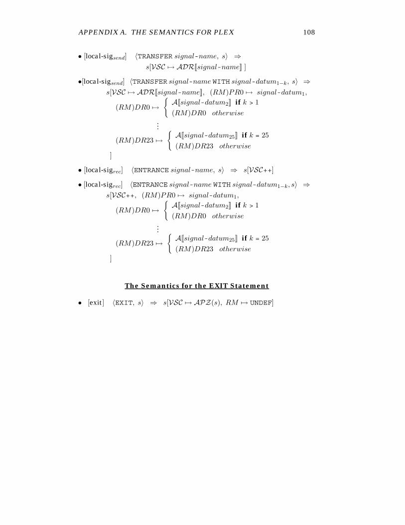
APPENDIX A. THE SEMANTICS FOR PLEX 108
• [local-sigsend] 〈TRANSFER signal-name, s〉 ⇒s[VSC �→ ADR[[signal-name]] ]
•[local-sigsend] 〈TRANSFER signal-name WITH signal-datum1−k, s〉 ⇒s[VSC �→ ADR[[signal-name]], (RM)PR0 �→ signal-datum1,
(RM)DR0 �→{
A[[signal-datum2]] if k > 1(RM)DR0 otherwise
...
(RM)DR23 �→{
A[[signal-datum25]] if k = 25(RM)DR23 otherwise
]
• [local-sigrec] 〈ENTRANCE signal-name, s〉 ⇒ s[VSC++]
• [local-sigrec] 〈ENTRANCE signal-name WITH signal-datum1−k, s〉 ⇒s[VSC++, (RM)PR0 �→ signal-datum1,
(RM)DR0 �→{
A[[signal-datum2]] if k > 1(RM)DR0 otherwise
...
(RM)DR23 �→{
A[[signal-datum25]] if k = 25(RM)DR23 otherwise
]
The Semantics for the EXIT Statement
• [exit] 〈EXIT, s〉 ⇒ s[VSC �→ APZ(s), RM �→ UNDEF]
Appendix B
The Signal Description
There are two main documents for signals: The Signal Survey, whichis a listing of all the signals sent and received in a unit, and the SignalDescription, which will be studied in this section. These documents arecompiled together with the Source Program Information1, SPI.
The Signal Description, SD, is the document that defines a signal.The type of the signal, as well as the priority level of the signal is speci-fied in this document. There is one SD for every signal and all SD’s arestored in special libraries. We will study how the SD ”interact” with theSPI during the code generation phase. But as a first attempt to capturethe contents of the SD, it could be seen as similar to the h-file in C
that externally defines a function (among other things).The SD includes the following items:
• Name of the signal - Every signal has a name that, perhaps,captures its functionality.
• Signal number - For internal documentation.
• Function - Used to make comments about functionality.
• Signal type - The signal type indicates whether the signal is Sin-gle or Combined. There are three possible type specifications:
– Type 1: Single signal1The Source Program Information is the ”source code file”, i.e., the document that
we normally call a program. See Section 2.2.1 for further details.

APPENDIX B. THE SIGNAL DESCRIPTION 110
– Type 2: Combined forward
– Type 3: Combined backward
If the signal is Multiple, this is indicated by adding the keywordMULTIPLE to the signal type, like in: TYPE IS 1 MULTIPLE
A Unique signal has no indication at this point! (A signal is unique”by default” if nothing else is stated.) If the signal is local, thekeyword LOCAL is added to the signal type.
• Possible return signal - For internal documentation.
• Possible sending block - For internal documentation.
• Possible receiving block - For internal documentation.
• Buffer level - The priority level! In Section 3.2, it is describedhow every signal is assigned a priority level, and how signals arestored in different job buffers (in case of a buffered signal). Thebuffer level states the priority level of the corresponding job andalso in which job buffer the signal will be buffered (if it is to bebuffered, i.e.).NOTE: The buffer level can have the following combinations:
– NO BUFFER: The signal is direct. (A combined signal isalways direct, see Section 3.1.3.)
– LEVEL A/B/C/D BUFFER: The signal is buffered and usesthe job buffer specified. This combination overrides a possibleuse of the HURRY option in the signal sending statement (seebelow).
– LEVEL A/B/C/D: The signal is buffered and uses the jobbuffer specified, unless the keyword HURRY is used in thesignal sending statement, which indicates that the signal isdirect.
• Signal data - Specification of the ”arguments” (i.e., the data) thatthe signal is carrying.
• ID sector - For internal documentation.