a stochastic volatility model with conditional skewess · a stochastic volatility model with...
TRANSCRIPT
Working Paper/Document de travail 2011-20
A Stochastic Volatility Model with Conditional Skewness
by Bruno Feunou and Roméo Tédongap
2
Bank of Canada Working Paper 2011-20
October 2011
A Stochastic Volatility Model with Conditional Skewness
by
Bruno Feunou1 and Roméo Tédongap2
1Financial Markets Department Bank of Canada
Ottawa, Ontario, Canada K1A 0G9 [email protected]
2Department of Finance
Stockholm School of Economics Stockholm, Sweden
Bank of Canada working papers are theoretical or empirical works-in-progress on subjects in economics and finance. The views expressed in this paper are those of the authors.
No responsibility for them should be attributed to the Bank of Canada.
ISSN 1701-9397 © 2011 Bank of Canada

ii
Acknowledgements
An earlier version of this paper was circulated and presented at various seminars and conferences under the title “Affine Stochastic Skewness.” We thank Nour Meddahi, Glen Keenleyside, Scott Hendry, seminar participants at the Duke University Financial Econometrics Lunch Group, participants at the Conference of the Society for Computational Economics (Montréal, June 2007), the Forecasting in Rio Conference at the Graduate School of Economics (Rio de Janeiro, July 2008), and the Summer Econometric Society Meetings (Boston University, June 2009).

iii
Abstract
We develop a discrete-time affine stochastic volatility model with time-varying conditional skewness (SVS). Importantly, we disentangle the dynamics of conditional volatility and conditional skewness in a coherent way. Our approach allows current asset returns to be asymmetric conditional on current factors and past information, what we term contemporaneous asymmetry. Conditional skewness is an explicit combination of the conditional leverage effect and contemporaneous asymmetry. We derive analytical formulas for various return moments that are used for generalized method of moments estimation. Applying our approach to S&P500 index daily returns and option data, we show that one- and two-factor SVS models provide a better fit for both the historical and the risk-neutral distribution of returns, compared to existing affine generalized autoregressive conditional heteroskedasticity (GARCH) models. Our results are not due to an overparameterization of the model: the one-factor SVS models have the same number of parameters as their one-factor GARCH competitors.
JEL classification: C1, C5, G1, G12 Bank classification: Econometric and statistical methods; Asset pricing
Résumé
Les auteurs élaborent un modèle discret affine à volatilité stochastique et asymétrie conditionnelle variable (modèle SVS). Leur approche a ceci d’intéressant qu’elle dissocie de façon cohérente la dynamique de la volatilité conditionnelle de celle de l’asymétrie conditionnelle. Elle permet une distribution asymétrique des rendements courants des actifs conditionnellement aux facteurs du moment et à l’information passée, asymétrie que les auteurs qualifient de « contemporaine ». Dans leur modèle, l’asymétrie conditionnelle découle de la combinaison explicite de l’effet de levier conditionnel et de l’asymétrie contemporaine. Les auteurs établissent les formules analytiques pour divers moments des rendements utiles pour l’estimation par la méthode des moments généralisés. En se servant de données relatives aux rendements journaliers de l’indice S&P 500 et aux options connexes, ils montrent que les modèles SVS à un et à deux facteurs décrivent mieux la distribution des rendements (tant historique que risque neutre) que les modèles GARCH affines existants. Leurs résultats ne tiennent pas à un surparamétrage, puisque les modèles SVS unifactoriels comptent le même nombre de paramètres que les modèles GARCH unifactoriels.
Classification JEL : C1, C5, G1, G12 Classification de la Banque : Méthodes économétriques et statistiques; Évaluation des actifs
1 Introduction
The option-pricing literature holds that generalized autoregressive conditional heteroskedasticity
(GARCH) and stochastic volatility (SV) models significantly outperform the Black-Scholes model.
However, SV models have traditionally been examined in continuous time and the literature has
paid less attention to discrete-time SV option valuation models. This is due to the limitations of
existing discrete-time SV models in capturing the characteristics of asset returns that are essential to
improve their fit of option data. In particular, these models commonly assume that the conditional
distribution of returns is symmetric, violate the positivity of the volatility process or do not allow for
leverage effects. This paper contributes to the literature by examining the implications of allowing
conditional asymmetries in discrete-time SV models.
The paper proposes and tests a parsimonious discrete-time affine model with stochastic volatility
and conditional skewness. Our focus on the affine class of financial time-series volatility models is
motivated by their tractability in empirical applications. In option pricing, for example, European
options admit closed-form prices. To the best of our knowledge, there is no discrete-time SV model
delivering a closed-form option price that has been empirically tested using option data, in contrast
to tests performed in several GARCH models. Heston and Nandi (2000) and Christoffersen et al.
(2006) describe examples of one-factor GARCH models that belong to the discrete-time affine class,
and feature the conditional leverage effect (both papers) and conditional skewness (only the latter
paper) in single-period returns. Christoffersen et al. (2008) provide a two-factor generalization
of Heston and Nandi’s (2000) model to long- and short-run volatility components. The model
features only the leverage effect but not conditional skewness in single-period returns. We compare
the performance of the new model to these benchmark GARCH models along several dimensions.
As pointed out by Christoffersen et al. (2006), conditionally nonsymmetric return innovations
are critically important, since in option pricing, for example, heteroskedasticity and the leverage
effect alone do not suffice to explain the option smirk. However, skewness in their inverse Gaussian
GARCH model is still deterministically related to volatility and both undergo the same return
shocks, while our proposed model features stochastic volatility. Existing GARCH and SV models
also characterize the relation between returns and volatility only through their contemporaneous
1
covariance (the so-called leverage effect). In contrast, our modeling approach characterizes the
entire distribution of returns conditional upon the volatility factors. We refer to the asymmetry of
that distribution as contemporaneous asymmetry, which adds up to the leverage effect to determine
conditional skewness.
We show that, in the case of affine models, all unconditional moments of observable returns can
be derived analytically. We develop and implement an algorithm for computing these unconditional
moments in a general discrete-time affine model that nests our proposed model and all existing
affine GARCH models. Jiang and Knight (2002) provide similar results in an alternative way for
continuous-time affine processes. They derive the unconditional joint characteristic function of the
diffusion vector process in closed form. In discrete time, this can be done only through calculation
of unconditional moments, and the issue has not been addressed so far in the literature. Analytical
formulas help in assessing the direct impact of model parameters on critical unconditional moments.
In particular, this can be useful for calibration exercises where model parameters are estimated to
directly match relevant sample moments from the data.
Armed with these unconditional moments, we propose a generalized method of moments (GMM)-
based estimation of affine GARCH and SV models based on exact moment conditions. Interestingly,
the sample variance-covariance matrix of the vector of moments is nonparametric, thus allowing
for efficient GMM in one step. This approach is faster and computationally more efficient than
alternative estimation methods (see Jacquier et al. 1994; Andersen et al. 1999; Danielsson 1994).
Moreover, the minimum distance between model-implied and actual sample return moments ap-
pears as a natural metric for comparing different model fits.
Applying this GMM procedure to fit the historical dynamics of observed returns from January
1962 to December 2010, we find that the SVS model characterizes S&P500 returns well. In addition
to the sample mean, variance, skewness and kurtosis of returns, the models are estimated to match
the sample autocorrelations of squared returns up to a six-month lag, and the correlations between
returns and future squared returns up to a two-month lag. The persistence and the size of these
correlations at longer lags cannot be matched by single-factor models. We find that the two-factor
models provide the best fit of these moments and, among them, the two-factor SVS model does
better than the two-factor GARCH model.
2
Our results point out the benefit of allowing for conditional skewness in returns, since the one-
factor SVS model with contemporaneous normality fits better than the GARCH model of Heston
and Nandi (2000), although both models share the same number of parameters. Our results also
show that the SVS model with contemporaneous normality is more parsimonious than the inverse
Gaussian GARCH model of Christoffersen et al. (2006), which has one more parameter and nests
the GARCH model of Heston and Nandi (2000). In fact, the SVS model with contemporaneous
normality and the inverse Gaussian GARCH model have an equal fit of the historical returns
distribution.
Fitting the risk-neutral dynamics using S&P500 option data, we find that explicitly allowing
for contemporaneous asymmetry in the one-factor SVS model leads to substantial gains in option
pricing, compared to benchmark one-factor GARCH models. We compare models using the option
implied-volatility root-mean-square error (IVRMSE). The one-factor SVS model with contempo-
raneous asymmetry outperforms the two benchmark one-factor GARCH models in the overall fit
of option data and across all option categories as well. The IVRMSE of the SVS model is about
23.26% and 19.85% below that of the GARCH models. The two-factor models show the best fit of
option data overall and across all categories, and they have a comparable fit overall. The two-factor
SVS model has an overall IVRMSE of 2.98%, compared to 3.00% for the two-factor GARCH model.
The rest of the paper is organized as follows. Section 2 discusses existing discrete-time affine
GARCH and SV models and their limitations. Section 3 introduces our discrete-time SVS model
and discusses the new features relative to existing models. Section 4 estimates univariate and
bivariate SVS and GARCH models on S&P500 index daily returns and provides comparisons and
diagnostics. Section 5 estimates univariate and bivariate SVS models, together with competitive
GARCH models, using S&P500 index daily option data, and provides comparisons and diagnostics.
Section 6 concludes. An external appendix containing additional materials and proofs is available
from the authors’ webpages.
3
2 Discrete-Time Affine Models: An Overview
A discrete-time affine latent-factor model of returns with time-varying conditional moments may
be characterized by its conditional log moment-generating function:
Ψt (x, y; θ) = lnEt
[exp
(xrt+1 + y>lt+1
)]= A (x, y; θ) +B (x, y; θ)> lt, (1)
where Et [·] ≡ E [· | It] denotes the expectation conditional on a well-specified information set It,
rt is the observable returns, lt = (l1t, .., lKt)> is the vector of latent factors and θ is the vector
of parameters. Note that the conditional moment-generating function is exponentially linear in
the latent variable lt only. Bates (2006) refers to such a process as semi-affine. In what follows,
the parameter θ is withdrawn from functions A and B for expositional purposes. In this section,
we discuss discrete-time affine GARCH and SV models and their limitations, which we want to
overcome by introducing a new discrete-time affine SV model featuring conditional skewness.
The following SV models are discrete-time semi-affine univariate latent-factor models of returns
considered in several empirical studies. The dynamics of returns is given by
rt+1 = µr − λhµh + λhht +√htut+1, (2)
where the volatility process satisfies one of the following:
ht+1 = (1− φh)µh − αh +(φh − αhβ2
h
)ht + αh
(εt+1 − βh
√ht
)2, (3)
ht+1 = (1− φh)µh + φhht + σhεt+1, (4)
ht+1 = (1− φh)µh + φhht + σh√htεt+1, (5)
and where ut+1 and εt+1 are two i.i.d. standard normal shocks. The parameter vector θ is
(µr, λh, µh, φh, αh, βh, ρrh)> with volatility dynamics (3), whereas it is (µr, λh, µh, φh, σh)> with au-
toregressive Gaussian volatility (4) and finally (µr, λh, µh, φh, σh, ρrh)> with square-root volatility
(5), where ρrh denotes the conditional correlation between the shocks ut+1 and εt+1. The special
case ρrh = 1 in the volatility dynamics (3) corresponds to Heston and Nandi’s (2000) GARCH
4
model, which henceforth we refer to as HN.
Note that volatility processes (4) and (5) are not well defined, since ht can take negative values.
This can also arise with process (3) unless the parameters satisfy a couple of constraints. In
simulations, for example, one should be careful when using a reflecting barrier at a small positive
number to ensure the positivity of simulated volatility samples. Besides, if the volatility shock εt+1
in (4) is allowed to be correlated to the return shock ut+1 in (2), then the model loses its affine
property. Also notice that the conditional skewness of returns in these models is zero.
Christoffersen et al. (2006) propose an affine GARCH model that allows conditional skewness
in returns, specified by
rt+1 = γh + νhht + ηhyt+1, (6)
ht+1 = wh + bhht + chyt+1 + ahh2t
yt+1, (7)
where, given the available information at time t, yt+1 has an inverse Gaussian distribution with the
degree-of-freedom parameter ht/η2h . Alternatively, yt+1 may be written as
yt+1 =htη2h
+
√htηh
zt+1, (8)
where zt+1 follows a standardized inverse Gaussian distribution with parameter st = 3ηh/√ht. The
standardized inverse Gaussian distribution is introduced in Section 3.1.1. Interestingly, Christof-
fersen et al. (2006) provide a reparameterization of their model so that HN appears to be a limit
as ηh approaches zero:
ah =αhη4h
, bh = φh −αhη2h
− αh − 2αhηhβhη2h
, ch = αh − 2αhηhβh,
wh = (1− φh)µh − αh, γh = µr − λhµh, νh = λh −1
ηh.
(9)
Henceforth we refer to this specification as CHJ.
While CHJ allows for both the leverage effect and conditional skewness, it does not separate
the volatility of volatility from the leverage effect on the one hand, and conditional skewness from
volatility on the other hand. In particular, conditional skewness and volatility are related by
5
st = 3ηh/√ht. In consequence, the sign of conditional skewness is constant over time and equal to
the sign of the parameter ηh. This contrasts with the empirical evidence in Harvey and Siddique
(1999) that conditional skewness changes sign over time. Feunou et al.’s (2011) findings also suggest
that, although conditional skewness is centered around a negative value, return skewness may take
positive values.
Christoffersen et al. (2008) introduce a two-factor generalization of HN to long- and short-run
volatility components, which henceforth we refer to as CJOW. In addition to the dynamics of return
(2), the volatility dynamics may be written as follows:
ht = h1,t + h2,t where
h1,t+1 = µ1h + φ1hh1,t + α1hu2t+1 − 2α1hβ1h
√htut+1
h2,t+1 = µ2h + φ2hh2,t + α2hu2t+1 − 2α2hβ2h
√htut+1,
(10)
with µ1h = 0, since only the sum µ1h + µ2h is identifiable.
Liesenfeld and Jung (2000) introduce SV models with conditional heavy tails, but their model
is non-affine. However, SV models with conditional asymmetry have received less attention so far.
In this paper, we aim to combine in a coherent way both the affine property and the ability of
an SV model to fit critical moments of the data (mean, variance, skewness, kurtosis, multiple-
day autocorrelation of squared returns and cross-correlation between returns are future squared
returns). In the next section, we develop an affine multivariate latent-factor model of returns such
that both conditional variance ht and conditional skewness st are stochastic. We refer to such
a model as SVS. The proposed model is parsimonious and solves for the limitations of existing
models. Later in Sections 4 and 5, we use S&P500 index returns and option data to examine the
relative performance of the one- and two-factor SVS to the GARCH alternatives (HN, CHJ and
CJOW).
3 Building an SV Model with Conditional Skewness
3.1 The Model Structure
For each variable in what follows, the time subscript denotes the date from which the value of the
variable is observed by the economic agent; to simplify notations, the usual scalar operators will
6

also apply to vectors element-by-element. The joint distribution of returns rt+1 and latent factors
σ2t+1 conditional on previous information denoted It and containing previous realizations of returns
rt = {rt, rt−1, ...} and latent factors σ2t = {σ2
t , σ2t−1, ...} may be decomposed as follows:
f(rt+1, σ
2t+1 | It
)≡ fc
(rt+1 | σ2
t+1, It)× fm
(σ2t+1 | It
). (11)
Based on this, our modeling strategy consists of specifying, in a first step, the distribution of returns
conditional on factors and previous information, and, in a second step, the dynamics of the factors.
The first step will be characterized by inverse Gaussian shocks, and the second step will follow a
multivariate autoregressive gamma process.
3.1.1 Standardized Inverse Gaussian Shocks
The dynamics of returns in our model is built upon shocks drawn from a standardized inverse
Gaussian distribution. The inverse Gaussian process has been investigated by Jensen and Lunde
(2001), Forsberg and Bollerslev (2002), and Christoffersen et al. (2006). See also the excellent
overview of related processes in Barndorff-Nielsen and Shephard (2001).
The log moment-generating function of a discrete random variable that follows a standardized
inverse Gaussian distribution of parameter s, denoted SIG (s), is given by
ψ (u; s) = lnE [exp (uX)] = −3s−1u+ 9s−2
(1−
√1− 2
3su
). (12)
For such a random variable, one has E [X] = 0, E[X2]
= 1 and E[X3]
= s, meaning that s is
the skewness of X. In addition to the fact that the SIG distribution is directly parameterized by
its skewness, the limiting distribution when the skewness s tends to zero is the standard normal
distribution, that is SIG (0) ≡ N (0, 1). This particularity makes the SIG an ideal building block
for studying departures from normality.
3.1.2 Autoregressive Gamma Latent Factors
The conditional distribution of returns is further characterized by K latent factors, the components
of the K-dimensional vector process σ2t+1. We assume that σ2
t+1 is a multivariate autoregressive
7

gamma process with mutually independent components. We use this process to guarantee the
positivity of the volatility factors so that volatility itself is well defined. Its cumulant-generating
function, conditional on It, is given by
Ψσt (y) ≡ lnE
[exp
(y>σ2
t+1
)| It]
=K∑i=1
fi (yi) +K∑i=1
gi (yi)σ2i,t,
fi (yi) = −νi ln (1− αiyi) and gi (yi) =φiyi
1− αiyi.
(13)
Each factor σ2i,t is a univariate autoregressive gamma process, which is an AR(1) process with
persistence parameter φi. The parameters νi and αi are related to persistence, unconditional
mean µi and unconditional variance ωi as νi = µ2i /ωi and αi = (1− φi)ωi /µi . A more in-depth
treatment of the univariate autoregressive gamma process can be found in Gourieroux and Jasiak
(2006) and Darolles et al. (2006). Their analysis is extended to the multivariate case and applied
to the term structure of interest rates modeling by Le et al. (2010). The autoregressive gamma
process also represents the discrete-time counterpart to the continuous-time square-root process
that has previously been examined in the SV literature (see, for example, Singleton 2006, p. 110).
We denote by mσt , vσt and ξσt the K-dimensional vectors of conditional means, variances, and
third moments of the individual factors, respectively. Their ith component is given by
mσi,t = (1− φi)µi + φiσ
2i,t and vσi,t = (1− φi)2 ωi +
2 (1− φi)φiωiµi
σ2i,t,
ξσi,t =2 (1− φi)3 ω2
i
µi+
6 (1− φi)2 φiω2i
µ2i
σ2i,t.
(14)
The AR(1) process σ2i,t thus has the formal representation
σ2i,t+1 = (1− φi)µi + φiσ
2i,t +
√vσi,tzi,t+1 (15)
where vσi,t is given in equation (14) and zi,t+1 is an error with mean zero and unit variance and
skewness ξσi,t
(vσi,t
)−3/2. The conditional density function of an autoregressive gamma process is
obtained as a convolution of the standard gamma and Poisson distributions. A discussion and a
formal expression of that density can be found in Singleton (2006, p. 109).
8
3.1.3 The Dynamics of Returns
Formally, we assume that logarithmic returns have the following dynamics:
rt+1 = lnPt+1
Pt= µrt + urt+1, (16)
where P is the price of the asset, µrt ≡ Et [rt+1 | It] denotes the expected (or conditional mean of)
returns, which we assume are given by
µrt = λ0 + λ>σ2t , (17)
and urt+1 ≡ rt+1 − Et [rt+1 | It] represents the unexpected (or innovation of) returns, which we
assume are given by
urt+1 = β>(σ2t+1 −mσ
t
)+ σ>t+1ut+1. (18)
Our modeling strategy thus decomposes unexpected returns into two parts: a contribution due to
factor innovations and another due to shocks that are orthogonal to factor innovations. We assume
that the ith component of this K-dimensional vector of shocks ut+1 has a standardized inverse
Gaussian distribution, conditional on factors and past information,
ui,t+1 |(σ2t+1, It
)∼ SIG
(ηiσ−1i,t+1
), (19)
and that the K return shocks are mutually independent conditionally on(σ2t+1, It
). If ηi = 0, then
ui,t+1 is a standard normal shock.
Under these assumptions, we have
lnE[exp (xrt+1) | σ2
t+1, It]
=(µrt − β>mσ
t
)x+
K∑i=1
(βix+ ψ (x; ηi))σ2i,t+1, (20)
where the function ψ (·, s) is the cumulant-generating function of the standardized inverse Gaussian
distribution with skewness s as defined in equation (12). In total, the model has 1+6K parameters
grouped in the vector θ =(λ0, λ
>, β>, η>, µ>, φ>, ω>)>. The scalar λ0 is the drift coefficient in
conditional expected returns. All vector parameters in θ are K-dimensional. Namely, the vector λ
9
contains loadings of expected returns on the K factors, the vector β contains loadings of returns
on the K factor innovations, the vector η contains skewness coefficients of the K standardized
inverse Gaussian shocks, and the vectors µ, φ and ω contain unconditional means, persistence and
variances of the K factors, respectively.
Although, for the purpose of this paper, we limit ourselves to a single-return setting, the model
admits a straightforward generalization to multiple returns. Also, we further limit our empirical
application in this paper to one and two factors. Since the empirical evidence regarding the time-
varying conditional mean is weak from historical index daily returns data, we will restrict ourselves
in the estimation section to λ = 0 and will pick λ0 to match the sample unconditional mean of
returns, leaving us with 5K critical parameters from which further interesting restrictions can be
considered.
3.2 Volatility, Conditional Skewness and the Leverage Effect
In the previous subsection, we did not model conditional volatility and skewness or other higher
moments of returns directly. Instead, we related returns to stochastic linearly independent positive
factors. In this section, we derive useful properties of the model and discuss its novel features in
relation to the literature. In particular, we show that, in addition to stochastic volatility and the
leverage effect, the model generates conditional skewness. This nonzero and stochastic conditional
skewness, coupled with the ability of the model to generalize to multiple returns and multiple
factors, constitutes the main significant difference from previous affine SV models in discrete time.
The conditional variance, ht, and the conditional skewness, st, of returns, rt+1, may be expressed
as follows:
ht ≡ Et[(rt+1 − µrt )
2 | It]
= ι>mσt +
(β2)>vσt =
K∑i=1
hi,t, (21)
sth3/2t ≡ Et
[(rt+1 − µrt )
3 | It]
= η>mσt + 3β>vσt +
(β3)>ξσt =
K∑i=1
%i,t, (22)
with
hi,t = c0i,h + ci,hσ2i,t and %i,t = c0i,s + ci,sσ
2i,t, (23)
10

where ι is the K-dimensional vector of ones, and the coefficients ci,h and ci,s depend on model
parameters θ. These coefficients are explicitly given by
c0i,h = (1− φi)(µi + (1− φi)ωiβ2
i
)and ci,h =
(1 +
2 (1− φi)ωiβ2i
µi
)φi,
c0i,s = (1− φi)
(ηiµi + 3 (1− φi)ωiβi +
2 (1− φi)2 ω2i β
3i
µi
),
ci,s =
(ηi +
6 (1− φi)ωiβiµi
+6 (1− φi)2 ω2
i β3i
µ2i
)φi.
(24)
Conditional on It, covariance between returns rt+1 and volatility ht+1 (the leverage effect) may
be expressed as:
Cov (rt+1, ht+1 | It) = (βch)> vσt =K∑i=1
ϑi,t with ϑi,t = c0i,rh + ci,rhσ2i,t, (25)
where ch = (c1,h, c2,h, . . . , cK,h)> and the coefficients ci,rh are explicitly given by
c0i,rh =
(1 +
2 (1− φi)ωiβ2i
µi
)(1− φi)2 φiωiβi,
ci,rh = 2
(1 +
2 (1− φi)ωiβ2i
µi
)(1− φi)φ2
iωiβiµi
.
(26)
It is not surprising that the parameter β alone governs the conditional leverage effect, since it
represents the slope of the linear projection of returns on factor innovations. In particular, for
the one-factor SVS model to generate a negative correlation between spot returns and variance
as postulated by Black (1976) and documented by Christie (1982) and others, the parameter β1
should be negative.
In our SVS model, contemporaneous asymmetry η, alone, does not characterize conditional
skewness, as shown in equation (22). The parameter β, which alone characterizes the leverage
effect, also plays a central role in generating conditional asymmetry in returns, even when η = 0.
In contrast to SV models discussed in Section 2, where the leverage effect generates skewness only
in the multiple-period conditional distribution of returns, in our setting it invokes skewness in the
single-period conditional distribution as well.
11
To better understand the flexibility of the SVS model in generating conditional skewness, we
consider the one-factor SVS without loss of generality. The left-hand side of the last equality in
equation (22) shows that conditional skewness is the sum of three terms. The first term has the
sign of η1 and the last two terms have the same sign of β1. A negative β1 is necessary to generate
the well-documented leverage effect. In that case, the last two terms in (22) are negative. The sign
of conditional skewness will then depend on η1. If η1 is zero or negative, then conditional skewness
is negative over time, as in CHJ. Note that conditional skewness may change sign over time if η1
is positive and c01,sc1,s < 0. There are lower and upper positive bounds on η1 such that this latter
condition holds. These bounds are, respectively, −3 (1− φ1)ω1β1/µ1 − 2 (1− φ1)2 ω21β
31/µ
21 and
−6 (1− φ1)ω1β1/µ1−6 (1− φ1)2 ω21β
31/µ
21. This shows that the one-factor SVS model can generate
a more realistic time series of conditional skewness compared to CHJ.
We acknowledge that extensions of the basic SV model in continuous time can capture the
stylized facts of daily asset prices just as well as the SVS model introduced in this paper. However,
the econometrics required for estimating continuous-time processes are demanding, because of
the complexity of the resulting filtering and sampling. The advantage of our discrete-time affine
approach is not only that it gives an alternative to discrete-time users, but also that discrete-time
GARCH and SV models provide straightforward tools to deal with estimation and inference. In
the external appendix, we show that although the current SVS model is written in discrete time
and is easily applicable to discrete data, it admits interesting continuous-time limits, including
the standard SV model of Heston (1993) and an SV model with a jump process with stochastic
intensity.
In the next section, we develop an estimation procedure for the one- and two-factor SVS models
together with their competitors, HN, CHJ and CJOW. We seek a unified framework where these
different models can be estimated and evaluated according to the same criteria, thereby facilitating
their empirical comparison. Our proposed framework uses the generalized method of moments to
estimate, test and compare the models under consideration. It exploits the affine property of the
models to compute analytically model-implied unconditional moments of returns that are further
compared to their empirical counterparts. We describe our approach in detail in the next section,
and in Section 5 we compare the option-pricing performance of the models.
12
4 SVS vs. GARCH Models: Time-Series Analysis
4.1 Analytical Expressions of Unconditional Moments
Given the joint conditional log moment-generating function (1) of returns and latent variables, the
unconditional log moment-generating function of the latent vector lt, denoted by Ψl (·), satisfies
Ψl (y) = Al (y) + Ψl (Bl (y)) , (27)
where Al (y) ≡ A (0, y) and Bl (y) ≡ B (0, y). Proof of equation (27) can be found in the external
appendix. The function Ψl (·) obtains analytically in some cases, for instance the affine jump-
diffusion processes, as in Jiang and Knight (2002). In a discrete-time setting, it is sufficient to find
the derivatives of Ψl (y) at y = 0, and this can be done through differentiation of equation (27).
We show that the nth unconditional cumulant of the latent vector lt is the Kn−1 ×K matrix
κl (n) ≡ κl (n) = DnΨl (0), where DnΨl (0) is the solution to the equation
DnΨl (0) = DnAl (0) + Dn (Ψl (Bl (y)))|y=0 , (28)
and depends on DΨl (0), D2Ψl (0),. . ., Dn−1Ψl (0), DBl (0), D2Bl (0),. . ., DnBl (0), and where the
operator D defines the Jacobian of a matrix function of a matrix variable, as in Magnus and
Neudecker (1988, p. 173).
The higher-order derivatives of the composite function in the right-hand side of equation (28)
are evaluated through the chain rule given by Faa di Bruno’s formula, of which the multivariate
version is discussed in detail in Constantine and Savits (1996). In the case of a univariate latent
variable (lt is scalar), it is easy to solve equation (28) for higher-order cumulants of the latent
variable. However, this task is more cumbersome and tedious when lt is a vector. In the latter
case, the solution to equation (28) for n = 1, which is for the first cumulant, is given by
DΨl (0) = DAl (0) [IdK −DBl (0)]−1 , (29)
where IdK denotes the K×K identity matrix and DBl (0) represents the persistence matrix of the
13
latent vector lt. When n > 1, which is for the second- and higher-order cumulant, it can be shown
that the matrix DnΨl (0) satisfies
DnΨl (0)−(
(DBl (0))⊗(n−1))>DnΨl (0)DBl (0) = DnAl (0) + Cn, (30)
where the matrix Cn depends on the matrices{DjBl (0)
}1≤j≤n−1
and{DjΨl (0)
}2≤j≤n through the
multivariate version of Faa di Bruno’s formula. For example, the second unconditional cumulant
of the latent vector is given by
D2Ψl (0)−DBl (0)>D2Ψl (0)DBl (0) = D2Al (0) + (IdK ⊗DΨl (0))D2Bl (0) . (31)
Equation (30) shows that DnΨl (0) is the solution to a matrix equation of the form X−∆XΓ =
Λ. The solution to that equation is given by
vec (X) =[Id−
(Γ> ⊗∆
)]−1vec (Λ) .
Moments and cross-moments of returns can also be computed analytically, and this can be per-
formed through cross-cumulants of couples (rt+1, rt+1+j)> , j > 0. The unconditional log moment-
generating function of such couples is easily obtained in the case of affine models (see Darolles et
al. 2006). It is given by
Ψr,j (x, z) = Ar,j (z) +A (x,Br,j (z)) + Ψl (B (x,Br,j (z))) , (32)
where the functions Ar,j and Br,j satisfy the forward recursions
Ar,j (z) = Ar,j−1 (z) +Al (Br,j−1 (z)) , (33)
Br,j (z) = Bl (Br,j−1 (z)) , (34)
with the initial conditions Ar,1 (z) = A (z, 0) and Br,1 (z) = B (z, 0).
Given n > 0 and m > 0, the unconditional cross-cumulant of order (n,m) of the observable
14
returns rt is the number κr,j (n,m) ≡ ∂n+mΨr,j∂xn∂zm (0, 0) where
∂n+mΨr,j∂xn∂zm (0, 0) is the solution to
∂n+mΨr,j
∂xn∂zm(0, 0) =
∂n+m
∂xn∂zm(A (x,Br,j (z)))
∣∣∣∣x=0,z=0
+∂n+m
∂xn∂zm(Ψl (B (x,Br,j (z))))
∣∣∣∣x=0,z=0
. (35)
Equation (35) shows that cumulants of the latent vector lt are essential to compute cumulants and
cross-cumulants of returns.
We have just provided analytical formulas for computing return cumulants and cross-cumulants
κr,j (n,m) , j > 0, n ≥ 0, m > 0. This also allows us to compute analytically the corresponding
return moments and cross-moments µr,j (n,m) = E[rnt r
mt+j
]through the relationship between
multivariate moments and cumulants.
4.2 GMM Procedure
All the moments previously computed are functions of the parameter vector θ that governs the joint
dynamics of returns and the latent factors. We can then choose N pertinent moments to perform
the GMM estimation of the returns model. In this paper, we choose N pertinent moments among
all the moments µr,j (n,m) = E[rnt r
mt+j
]such that j ≥ 1 , n ≥ 0 and m > 0. Since the moments
of observed returns implied by a given model can directly be compared to their sample equivalent,
our estimation setup evaluates the performance of a given model in replicating well-known stylized
facts.
Let gt (θ) =[rnit r
mit+ji− µr,ji (ni,mi)
]1≤i≤N
denote the N×1 vector of the chosen moments. We
have E [gt (θ)] = 0 and we define the sample counterpart of this moment condition as follows:
g (θ) =
E[rn1t r
m1t+j1
]− µr,j1 (n1,m1)
. . .
E[rnNt rmNt+jN
]− µr,jN (nN ,mN )
. (36)
Given the N ×N matrix W used to weight the moments, the GMM estimator θ of the parameter
vector is given by
θ = arg minθ
T(g (θ)> W g (θ)
), (37)
15
where T is the sample size. Interestingly, the heteroskedasticity and autocorrelation (HAC) esti-
mator of the variance-covariance matrix of gt (θ) is simply that of the variance-covariance matrix
of[rnit r
mit+ji
]1≤i≤N
, which does not depend on the vector of parameter θ. This is an advantage,
since with a nonparametric empirical variance-covariance matrix of moment conditions, the optimal
GMM procedure can be implemented in one step. It is also important to note that two different
models can be estimated via the same moment conditions and weighting matrix. Only the model-
implied moments [µr,ji (ni,mi)]1≤i≤N differ from one model to another in this estimation procedure.
In this case, the minimum value of the GMM objective function itself is a criterion for comparison
of the alternative models, since it represents the distance between the model-implied moments and
the actual moments.
We weigh the moments using the inverse of the diagonal of their long-run variance-covariance
matrix:
W ={Diag
(V ar [gt]
)}−1.
This matrix is nonparametric and puts more weight on moments with low magnitude. If the number
of moments to match is large, as is the case in our estimation in the next section, then inverting the
long-run variance-covariance matrix of moments will be numerically unstable. Using the inverse
of the diagonal instead of the inverse of the long-run variance-covariance matrix itself allows for
numerical stability if the number of moments to match is large, since inverting a diagonal matrix
is simply taking the diagonal of the inverse of its diagonal elements. The distance to minimize
reduces toN∑i=1
E[rnit r
mit+ji
]− E
[rnit r
mit+ji
]σ[rnit r
mit+ji
]/√T
2
, (38)
where observed moments are denoted with a hat and the model-implied theoretical moment without.
In some cases, this GMM procedure has a numerical advantage compared to the maximum-
likelihood estimation even when the likelihood function can be derived. Maximum-likelihood es-
timation becomes difficult to perform numerically and theoretically, especially when the support
of the likelihood function is parameter-dependent. While the appeal of GARCH models relies on
the availability of their likelihood function in analytical form, which eases their estimation, the
16
support of the likelihood function for CHJ is parameter-dependent. This complicates its estimation
by maximum likelihood and, most importantly, its inference. In fact, there exists no general theory
in the statistical literature about the distributional properties of the maximum-likelihood estimator
when the support of the likelihood function is parameter-dependent.
On the other hand, the maximum-likelihood estimation of semi-affine latent variable models of
Bates (2006) and the quasi-maximum-likelihood estimation based on the Kalman recursion have
the downside that critical unconditional higher moments (skewness and kurtosis) of returns can be
poorly estimated due to the second-order approximation of the distribution of the latent variable
conditional on observable returns. Moreover, in single-stage estimation and filtering methods such
as the unscented Kalman filter and Bates’s (2006) algorithm, approximations affect both parameter
and state estimations.
Conversely, our GMM procedure matches critical higher moments exactly and requires no ap-
proximation for parameter estimation. Given GMM estimates of model parameters, Bates’s (2006)
procedure, or any other filtering procedure, such as the unscented Kalman filter, can be followed for
the state estimation. In this sense, approximations required by these techniques affect only state
estimation.
4.3 Data and Parameter Estimation
Using daily returns on the S&P500 equal-weighted index from January 2, 1962 to December 31,
2010, we estimate the 5-parameter unconstrained one-factor SVS model, the 4-parameter one-
factor SVS model with the constraint η1 = 0 (contemporaneous normality), and the 10-parameter
unconstrained two-factor SVS model, which we respectively denote SVS1FU, SVS1FC and SVS2FU.
We also estimate their GARCH competitors, the one-factor models CHJ with five parameters and
HN with four parameters, and the two-factor model CJOW with seven parameters.
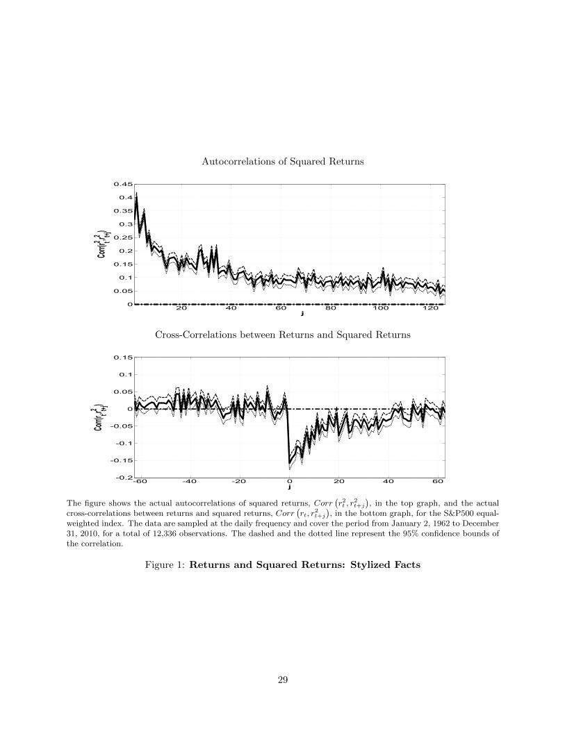
To perform the GMM procedure, we need to decide which moments to consider. The top panel
of Figure 1 shows that autocorrelations of daily squared returns are significant up to more than a
six-month lag (126 trading days). The bottom panel shows that correlations between daily returns
and future squared returns are negative and significant up to a two-month lag (42 trading days).
We use these critical empirical facts as the basis for our benchmark estimation. We then consider
17
the moments {E[r2t r
2t+j
]}j=1 to 126
and{E[rtr
2t+j
]}j=1 to 42
.
The return series has a standard deviation of 8.39E-3, a skewness of -0.8077 and an excess kurtosis
of 15.10, and these sample estimates are all significant at the 5% level. We then add the moments
{E [rnt ]}n=2 to 4
in order to match this significant variance, skewness and kurtosis. Thus, in total, our benchmark
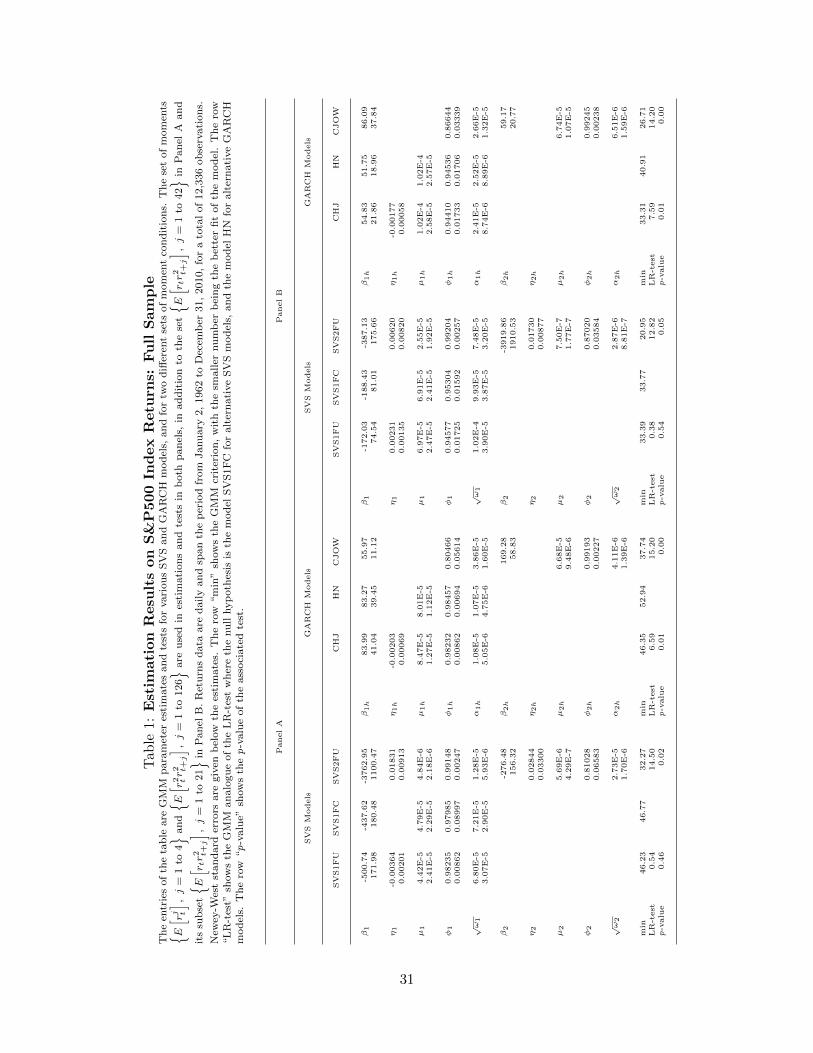
estimation uses 126+42+3=171 moments and the corresponding results are provided in Panel A of
Table 1.
Starting with the SVS model, Panel A of Table 1 shows that β1 is negative for the one-factor
SVS and both β1 and β2 are negative for the two-factor SVS. These coefficients are all significant
at conventional levels, as well as all the coefficients describing the factor dynamics. The SVS model
thus generates the well-documented negative leverage effect. Contemporaneous asymmetry does not
seem to be important for the historical distribution of returns. For the one-factor SVS model, the
minimum distance between actual and model-implied moments is 46.23 when η1 is estimated, and
46.77 when η1 is constrained to zero. The difference of 0.54 that follows a χ2 (1) is not statistically
significant, since its p-value of 0.46 is larger than conventional levels.
The minimum distance between actual and model-implied moments is 32.27 for the SVS2FU
model. The difference from the SVS1FC model is then 14.50 and follows a χ2 (6). It appears to
be statistically significant, since the associated p-value is 0.02, showing that the SVS2FU model
outperforms the one-factor SVS model. The SVS2FU model has a long-run volatility component
with a persistence of 0.99148, a half-life of 81 days, as well as a short-run volatility component
with a persistence of 0.81028, a half-life of approximately three days. The factor persistence in
the one-factor SVS model, 0.98235 for the SVS1FU and 0.97985 for the SVS1FC, is intermediate
between these long- and short-run volatility components, having a half-life of 39 days and 34 days,
respectively.
Panel A of Table 1 also shows results for the GARCH models. All parameters are statistically
significant at conventional levels and the parameter η1h is negative by our new estimation strategy,
18
corroborating the findings of Christoffersen et al. (2006). In addition, the “LR-test” largely rejects
HN against both CHJ and CJOW, with p-values lower than or equal to 2%, suggesting that
conditional skewness as well as more than one factor are both important features of the historical
returns distribution. It is important to note that the long- and short-run volatility components
implied by CJOW have persistence, 0.99193 and 0.80466, comparable to those of their analogue
implied by the SVS2FU model, 0.99148 and 0.81028 respectively. The volatility persistence in CHJ
and HN, 0.98232 and 0.98457 respectively, is also intermediate between the long- and short-run
volatility components.
Although the SVS1FC model and HN have the same number of parameters, the fit of actual
moments is different. The fit is better for the SVS1FC model, 46.77, compared to 52.94 for HN,
a substantial difference of 6.17, attributable to conditional skewness in the SVS1FC model. Also
note that the fit of the SVS1FC model and CHJ is comparable, 46.77 against 46.35, although the
SVS1FC has one less parameter. Non-reported results show that several constrained versions of
the two-factor SVS model cannot be rejected against the SVS2FU model, and they all outperform
CJOW as well. We examine one of these constrained versions in more detail in the option-pricing
empirical analysis.
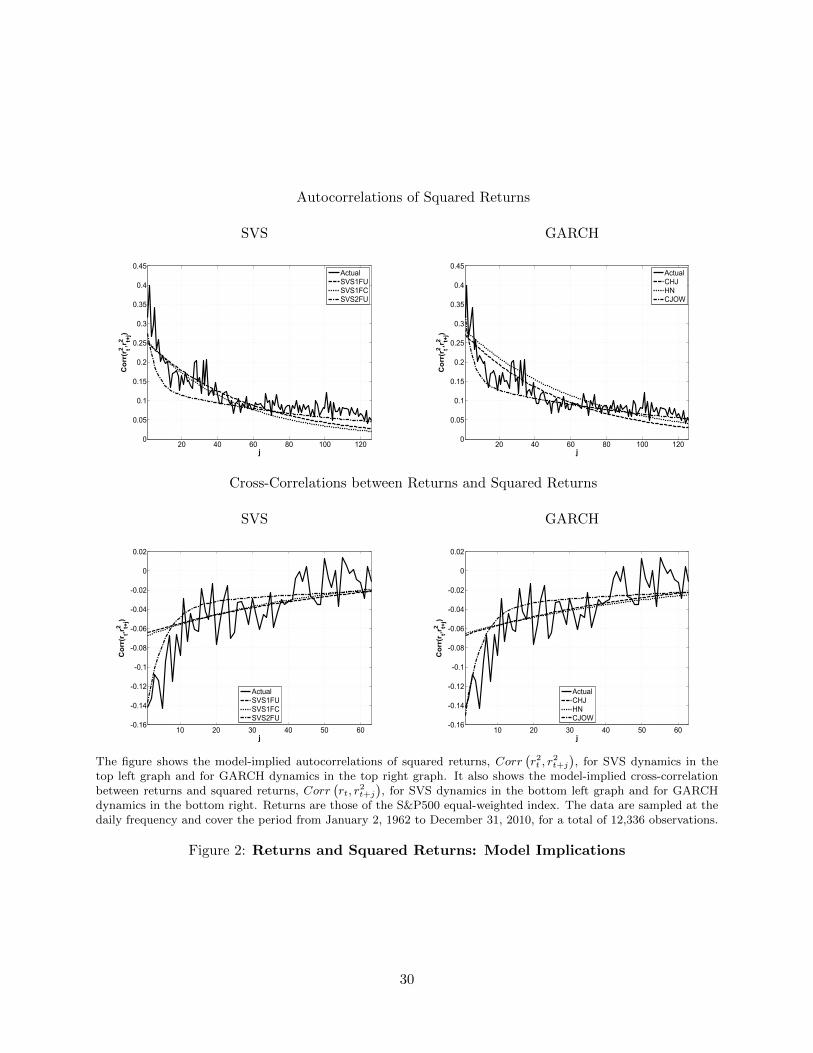
To further visualize how well the models reproduce the stylized facts, we complement the results
in Panel A of Table 1 by plotting the model-implied autocorrelations and cross-correlations together
with actual ones in Figure 2, for both SVS and GARCH. The figure highlights the importance of
a second factor in matching autocorrelations and cross-correlations at both the short and the long
horizons. In particular, a second factor is necessary to match long-horizon autocorrelations and
cross-correlations.
Panel B of Table 1 shows the estimation results when we decide to match the correlations
between returns and future squared returns up to only 21 days instead of the 42 days in Panel
A. In Panel B, we therefore eliminate 21 moments from the estimation. All the findings in Panel
A still hold in Panel B. In the external appendix, a table shows the estimation results over the
subsample starting January 2, 1981. All findings reported for the full sample are confirmed over
this subsample.
19
5 SVS vs. GARCH Models: Option-Pricing Analysis
5.1 Option Pricing with Stochastic Skewness
In this section, we assume that both GARCH and SVS dynamics are under the risk-neutral measure.
Hence we have
E [exp (rt+1) | It] = exp (rf ) , (39)
where rt+1 and rf refer to the risky return and the constant risk-free rate from date t to date
t + 1, respectively. In particular, for the SVS model, the pricing restriction (39) implies that the
coefficients λ0 and λi, i = 1, . . . ,K are given by
λ0 = rf +K∑i=1
νi (βiαi + ln (1− αi (βi + ψ(1; ηi)))) ,
λi = φi
(βi −
βi + ψ(1; ηi)
1− α (βi + ψ(1; ηi))
), i = 1, . . . ,K.
Because all models considered in this paper are affine, the price at date t of a European call option
with strike price X and maturity τ admits a closed-form formula, reported in the external appendix
owing to space limitations. We next discuss the option data used in our empirical analysis. Then
we estimate the models by maximizing the fit to our option data.
5.2 Option Data
We use closing prices on European S&P500 index options from OptionMetrics for the period January
1, 1996 through December 31, 2004. In order to ensure that the contracts we use are liquid, we rely
on only options with maturity between 15 and 180 days. For each maturity on each Wednesday, we
retain only the seven most liquid strike prices. We restrict attention to Wednesday data to enable
us to study a fairly long time-period while keeping the size of the data set manageable. Our sample
has 10,138 options. Using Wednesday is common practice in the literature, to limit the impact of
holidays and day-of-the week effects (see Heston and Nandi 2000; Christoffersen and Jacobs 2004).
Table 2 describes key features of the data. The top panel of Table 2 sorts the data by six mon-
20
eyness categories and reports the number of contracts, the average option price, the average Black-
Scholes implied volatility (IV), and the average bid-ask spread in dollars. Moneyness is defined
as the implied index futures price, F , divided by the option strike price X. The implied-volatility
row shows that deep out-of-the-money puts, those with F/X > 1.06, are relatively expensive. The
implied-volatility for those options is 25.73%, compared with 19.50% for at-the-money options. The
data thus display the well-known smirk pattern across moneyness. The middle panel sorts the data
by maturity reported in calendar days. The IV row shows that the term structure of volatility is
roughly flat, on average, during the period, ranging from 20.69% to 21.87%. The bottom panel
sorts the data by the volatility index (VIX) level. Obviously, option prices and IVs are increasing
in VIX, and dollar spreads are increasing in VIX as well. More importantly, most of our data are
from days with VIX levels between 15% and 35%.
5.3 Estimating Model Parameters from Option Prices
As is standard in the derivatives literature, we next compare the option-pricing performance of
HN, CHJ, CJOW, SVS1FU, SVS1FC, SVS2FU and the 8-parameter two-factor model with the
constraints η1 = 0 and β2 = 0, which we further denote as SVS2FC. We use the implied-volatility
root mean squared error (IVRMSE) to measure performance. Renault (1997) discusses the benefits
of using the IVRMSE metric for comparing option-pricing models. To obtain the IVRMSE, we
invert each computed model option price CModj using the Black-Scholes formula, to get the implied
volatility IVModj . We compare these model IVs to the market IV from the option data set, denoted
IVMarketj , which is also computed by inverting the Black-Scholes formula. The IVRMSE is now
computed as
IV RMSE ≡
√√√√ 1
N
N∑j=1
e2j , (40)
where ej ≡ IVMktj − IVMod
j and where N denotes the total number of options in the sample. We
estimate the risk-neutral parameters by maximizing the Gaussian IV option-error likelihood:
lnLO ∝ −1
2
N∑j=1
(ln(IV RMSE2
)+ e2
j/IV RMSE2). (41)
21
Model option prices CModj depend on time-varying factors. In the GARCH option-pricing
literature, it is standard to compute the volatility process using the GARCH volatility recursion,
since the factors are observable. Factors in the SVS models, however, are latent, and we need to filter
them in order to price options. To remain consistent and facilitate comparison with the GARCH
alternative, we develop a simple GARCH recursion that approximates the volatility dynamics in
the SVS model by matching the mean, variance, persistence and covariance with the returns of
each volatility component. The dynamics of each volatility component is then approximated using
Heston and Nandi’s (2000) GARCH recursion (3), where the GARCH coefficients are expressed in
terms of the associated SVS factor coefficients, as follows:
µih = µi +(1− φ2
i
)ωiβ
2i and φih = φi, (42)
αih = φi
√µiωi
(1− φ2
i
)2µih
(1 +
2 (1− φi)ωiβ2i
µi
)and βih = −βi
√(1− φ2
i
)ωi
2µiµih. (43)
Our matching procedure can be viewed as a second-order GARCH approximation of the SVS
dynamics, intuitively analogue to the approximation of the log characteristic function used by
Bates (2006) when filtering affine latent processes.
The top panel of Table 3 reports the results of the option-based estimation for SVS models, and
the bottom panel reports the results of the GARCH alternative. All parameters are significantly
estimated at the 1% level. Compared to historical parameters, the risk-neutral dynamics is more
negatively skewed and the variance components are more persistent. These two findings are very
common in the option-pricing literature. Higher negative skewness of the risk-neutral dynamics is
reflected in higher negative values of βi and ηi estimates for SVS models, and a larger negative
value of βih estimates for GARCH models. For example, the estimated values of β1 and η1 for
the SVS1FU model are, respectively, -2450 and -0.2325 for the risk-neutral dynamics in Table 3,
compared to -500 and -0.00364 respectively for the historical dynamics in Panel A of Table 1.
The persistence of the variance for the SVS1FU model is 0.9920 for the risk-neutral dynamics in
Table 3 and 0.9824 for the historical dynamics in Panel A of Table 1. The risk-neutral variance is
more persistent than the physical variance. Also, note that, for the SVS2FU model, both volatility
components are now very persistent under the risk-neutral dynamics, with half-lives of 30 days for
22
the short-run component and 385 days for the long-run component, compared to 3 days and 81
days, respectively, under the historical dynamics.
The last three rows of each panel in Table 3 show the log likelihood, the IVRMSE metric of
the models and their ratios relative to HN. The IVRMSE for the restricted one-factor SVS model,
SVS1FC, outperforms its one-factor GARCH competitors, HN and CHJ. The IVRMSE for the
SVS1FC model is 3.56%, compared with 3.89% and 3.78% for HN and CHJ, corresponding to
an improvement of 9.38% and 6.35%, respectively. Moving to the unrestricted one-factor SVS
model, SVS1FU, considerably reduces the pricing error and yields an impressive improvement of
23.26% and 19.85% over HN and CHJ, respectively. This result illustrates the superiority of our
conditional skewness modeling approach over existing affine GARCH, since CHJ has the same
number of parameters as the SVS1FU model, and more than the SVS1FC model. This result
also highlights the clear benefit of allowing more negative skewness in the risk-neutral conditional
distribution of returns.
Not surprisingly, the two-factor GARCH model (i.e., CJOW), with a RMSE of 3.00%, fits the
option data better than the one-factor GARCH and SVS models combined. In fact, as pointed out
by Christoffersen et al. (2008) and Christoffersen et al. (2009), a second volatility factor is needed to
fit appropriately the term structure of risk-neutral conditional moments. Our restricted two-factor
SVS model, SVS2FC, has a comparable fit to CJOW, with a RMSE of 2.98%. The performance of
the unconstrained two-factor SVS model is almost similar to the constrained version, reflecting the
fact that both η1 and β2 are not significantly estimated at the conventional 5% level. Option pricing
thus seems to favor a risk-neutral distribution of stock prices that features a Gaussian as well as
a negatively skewed shock; i.e., a discrete-time counterpart to a continuous-time jump-diffusion
model.
Overall, the results of model estimation based on option data confirm the main conclusions from
the GMM estimation based on returns in Section 4.3. Both conditional skewness in returns and
a second volatility factor are necessary to reproduce the observed stylized facts, and disentangling
the dynamics of conditional volatility from the dynamics of conditional skewness offers substantial
improvement in fitting the distribution of asset prices.
In Table 4, we dissect the overall IVRMSE results reported in Table 3 by sorting the data by
23
moneyness, maturity and VIX levels, using the bins from Table 2. The top panel of Table 4 reports
the IVRMSE for the seven models by moneyness. We see that the two-factor models, with the lowest
overall IVRMSE in Table 3, also have the lowest IVRMSE in each of the six moneyness categories.
The benefits offered by the two-factor models are therefore not restricted to any particular subset
of strike prices. Note that all models tend to perform worst for deep out-of-the-money put options
(F/X > 1.06), also corresponding to the highest average implied volatility, as shown by the top
panel of Table 2. For example, HN, CHJ and the SVS1FC model fit deep OTM options with
IVRMSEs of 5.54%, 5.25% and 5.04%, respectively. With a fit of 4.02%, CJOW is outperformed
by the SVS1FU, the SVS2FC and the SVS2FU models, which have fits of 3.81%, 3.60% and 3.58%,
respectively.
For deep-in-the-money options (F/X < 0.96), CJOW has the best fit, an IVRMSE of 2.99%,
compared to more than 3.31% for any other concurrent model. For all other moneyness categories,
CJOW and the two-factor SVS models have comparable fits, the difference in their IVRMSEs
being less than 0.10%. The performance of the SVS1FU model is very consistent across strikes as
well, the best among the one-factor models. Thus, contrary to the historical dynamics of returns,
contemporaneous asymmetry appears to be important in characterizing the risk-neutral dynamics,
and the low IVRMSE of the SVS1FU model compared to the SVS1FC model across all categories
demonstrates the impact of the significant and negative estimate of η1 reported in Table 3.
The middle panel of Table 4 reports the IVRMSE across maturity categories. Again we see that
all two-factor models have a comparable fit across all maturity categories, but the shortest maturity
(DTM < 30) where the two-factor SVS models perform better compared to CJOW. The SVS1FU
model still outperforms any other one-factor competitor along the maturity dimension. While
all models have relatively more difficulty fitting the shortest and the longest maturity compared
to intermediate maturity options, our results show the superiority of the SVS over the GARCH
regarding the shortest maturity options. With an IVRMSE of 3.14% for this category, the SVS1FU
model provides the best SVS fit, while the best GARCH fit of 3.66% is due to CJOW.
The bottom panel of Table 4 reports the IVRMSE across VIX levels. The two-factor models
provide the best fit across the six VIX categories, and the SVS1FU model remains the best one-
factor fit along this dimension. All models have difficulty fitting options when the level of market
24
volatility is high (V IX ≥ 35%), since, for all models, the IVRMSE is the highest for these VIX
levels.
To summarize, our option results show that, focusing on single-factor models, the empirical
performance of the SVS is superior to that of affine GARCH models in fitting the risk-neutral
distribution of asset prices inferred from option data. However, while the two-factor affine GARCH
model is comparable to the two-factor SVS in the overall fit, results across different option categories
are mixed.
6 Conclusion and Future Work
This paper presents a new approach for modeling conditional skewness in a discrete-time affine
stochastic volatility model. The model explicitly allows returns to be asymmetric conditional
on factors and past information. This contemporaneous asymmetry is shown to be particularly
important for the model to fit option data. An empirical investigation suggests that the flexibility
that the model offers for conditional skewness increases its option-pricing performance relative to
existing affine GARCH models. In particular, the one-factor SVS model with contemporaneous
asymmetry outperforms existing one-factor affine GARCH models across all option categories.
The paper also develops a methodology for estimating the historical distribution parameters of
a multivariate latent-factor model that nests the proposed SVS as well as existing affine GARCH
models. The setting allows for model comparison along the same statistics, the minimum distance
between model-implied and actual sample return moments.
In future research, it would be interesting to study the implications of the model for a parsi-
monious multiple-returns setting as well. An interesting exercise would be to look at “skewness
transmission” among international stock markets.
25

References
Andersen, T. G., Chung, H. J., and Sorensen, B. E. (1999), “Efficient Method of Moments Es-
timation of a Stochastic Volatility Model: A Monte Carlo Study,” Journal of Econometrics,
91, 61–87.
Barndorff-Nielsen, O. E., and Shephard, N. (2001), “Non-Gaussian Ornstein-Uhlenbeck-Based
Models and Some of Their Uses in Financial Economics,” Journal Of The Royal Statistical
Society Series B, 63 (2), 167–241.
Bates, D. S. (2006), “Maximum Likelihood Estimation of Latent Affine Processes,” Review of
Financial Studies, 19 (3), 909–965.
Black, F. (1976), “Studies of Stock Price Volatility Changes,” in Proceedings of the 1976 Meetings
of the American Statistical Association, Business and Economic Statistics Section, pp. 177–181.
Christie, A. A. (1982), “The Stochastic Behavior of Common Stock Variances: Value, Leverage
and Interest Rate Effects,” Journal of Financial Economics, 10 (4), 407–432.
Christoffersen, P., and Jacobs, K. (2004), “Which GARCH Model for Option Valuation?,” Man-
agement Science, 50 (9), 1204–1221.
Christoffersen, P., Heston, S., and Jacobs, K. (2006), “Option Valuation With Conditional Skew-
ness,” Journal of Econometrics, 131 (1-2), 253–284.
(2009), “The Shape and Term Structure of the Index Option Smirk: Why Multifactor Stochastic
Volatility Models Work So Well,” Management Science, 55 (12), 1914–1932.
Christoffersen, P., Jacobs, K., Ornthanalai, C., and Wang, Y. (2008), “Option Valuation With
Long-Run and Short-Run Volatility Components,” Journal of Financial Economics, 90 (3), 272–
297.
Constantine, G. M., and Savits, T. H. (1996), “A Multivariate Faa di Bruno Formula with Appli-
cations,” Transactions of the American Mathematical Society, 348 (2), 503–520.
26
Danielsson, J. (1994), “Stochastic Volatility in Asset Prices Estimation with Simulated Maximum
Likelihood,” Journal of Econometrics, 64 (1-2), 375–400.
Darolles, S., Gourieroux, C., and Jasiak, J. (2006), “Structural Laplace Transform and Compound
Autoregressive Models,” Journal of Time Series Analysis, 27 (4), 477–503.
Feunou, B., Jahan-Parvar, M. R., and Tedongap, R. (2011), “Modeling Market Downside Volatil-
ity,” Review of Finance, in press.
Forsberg, L., and Bollerslev, T. (2002), “Bridging the Gap Between the Distribution of Realized
(ECU) Volatility and ARCH Modelling (of the Euro): the GARCH-NIG Model,” Journal of
Applied Econometrics, 17 (5), 535–548.
Gourieroux, C., and Jasiak, J. (2006), “Autoregressive Gamma Processes,” Journal of Forecasting,
25 (2), 129–152.
Harvey, C. R., and Siddique, A. (1999), “Autoregressive Conditional Skewness,” Journal of Finan-
cial and Quantitative Analysis, 34 (04), 465–487.
Heston, S. (1993), “A Closed-Form Solution for Options with Stochastic Volatility with Applications
to Bond and Currency Options,” Review of Financial Studies, 6 (2), 327–343.
Heston, S., and Nandi, S. (2000), “A Closed-Form GARCH Option Valuation Model,” Review of
Financial Studies, 13 (3), 585–625.
Jacquier, E., Polson, N. G., and Rossi, P. E. (1994), “Bayesian Analysis of Stochastic Volatility
Models,” Journal of Business & Economic Statistics, 12 (4), 371–389.
Jensen, M. B., and Lunde, A. (2001), “The NIG-S&ARCH Model: A Fat-Tailed, Stochastic, and
Autoregressive Conditional Heteroskedastic Volatility Model,” Econometrics Journal, 4 (2), 319–
342.
Jiang, G. J., and Knight, J. L. (2002), “Estimation of Continuous-Time Processes via the Empirical
Characteristic Function,” Journal of Business & Economic Statistics, 20 (2), 198–212.
27
Le, A., Singleton, K. J., and Dai, Q. (2010), “Discrete-Time Affine Term Structure Models with
Generalized Market Prices of Risk,” Review of Financial Studies, 23 (5), 2184–2227.
Liesenfeld, R., and Jung, R. C. (2000), “Stochastic Volatility Models: Conditional Normality versus
Heavy-Tailed Distributions,” Journal of Applied Econometrics, 15 (2), 137–160.
Magnus, J., and Neudecker, H. (1988) Matrix Differential Calculus with Applications in Statistics
and Econometrics, Chichester, U.K: Wiley Series in Probability and Statistics.
Renault, E. (1997) “Econometric Models of Option Pricing Errors,” in Advances in Economics and
Econometrics: Theory and Applications, Seventh World Congress, eds. D.M. Kreps and K.F.
Wallis, Cambridge: Cambridge University Press, pp. 223-278.
Singleton, K. J. (2006) Empirical Dynamic Asset Pricing: Model Specification and Econometric
Assessment, Princeton, NJ: Princeton University Press.
28
Autocorrelations of Squared Returns
20 40 60 80 100 1200
0.05
0.1
0.15
0.2
0.25
0.3
0.35
0.4
0.45
j
Corr(r t2 ,r
t+j
2)
Cross-Correlations between Returns and Squared Returns
-60 -40 -20 0 20 40 60-0.2
-0.15
-0.1
-0.05
0
0.05
0.1
0.15
j
Corr(r t,r
t+j
2)
The figure shows the actual autocorrelations of squared returns, Corr(r2t , r
2t+j
), in the top graph, and the actual
cross-correlations between returns and squared returns, Corr(rt, r
2t+j
), in the bottom graph, for the S&P500 equal-
weighted index. The data are sampled at the daily frequency and cover the period from January 2, 1962 to December31, 2010, for a total of 12,336 observations. The dashed and the dotted line represent the 95% confidence bounds ofthe correlation.
Figure 1: Returns and Squared Returns: Stylized Facts
29
Autocorrelations of Squared Returns
SVS GARCH
20 40 60 80 100 1200
0.05
0.1
0.15
0.2
0.25
0.3
0.35
0.4
0.45
j
Corr(rt2,rt+j
2)
Actual
SVS1FU
SVS1FC
SVS2FU
20 40 60 80 100 1200
0.05
0.1
0.15
0.2
0.25
0.3
0.35
0.4
0.45
j
Corr(rt2,rt+j
2)
Actual
CHJ
HN
CJOW
Cross-Correlations between Returns and Squared Returns
SVS GARCH
10 20 30 40 50 60-0.16
-0.14
-0.12
-0.1
-0.08
-0.06
-0.04
-0.02
0
0.02
j
Corr(rt,r t+j
2)
Actual
SVS1FU
SVS1FC
SVS2FU
10 20 30 40 50 60-0.16
-0.14
-0.12
-0.1
-0.08
-0.06
-0.04
-0.02
0
0.02
j
Corr(rt,r t+j
2)
Actual
CHJ
HN
CJOW
The figure shows the model-implied autocorrelations of squared returns, Corr(r2t , r
2t+j
), for SVS dynamics in the
top left graph and for GARCH dynamics in the top right graph. It also shows the model-implied cross-correlationbetween returns and squared returns, Corr
(rt, r
2t+j
), for SVS dynamics in the bottom left graph and for GARCH
dynamics in the bottom right. Returns are those of the S&P500 equal-weighted index. The data are sampled at thedaily frequency and cover the period from January 2, 1962 to December 31, 2010, for a total of 12,336 observations.
Figure 2: Returns and Squared Returns: Model Implications
30
Tab
le1:
Est
imati
on
Resu
lts
on
S&
P500
Ind
ex
Retu
rns:
Fu
llS
am
ple
Th
een
trie
sof
the
tab
leare
GM
Mp
ara
met
eres
tim
ate
san
dte
sts
for
vari
ou
sS
VS
an
dG
AR
CH
mod
els,
an
dfo
rtw
od
iffer
ent
sets
of
mom
ent
con
dit
ion
s.T
he
set
of
mom
ents
{ E[ rj t
] ,j
=1
to4} a
nd{ E
[ r2 tr2 t+j
] ,j
=1
to126} a
reu
sed
ines
tim
ati
on
san
dte
sts
inb
oth
pan
els,
inad
dit
ion
toth
ese
t{ E
[ r tr2 t+j
] ,j
=1
to42} in
Pan
elA
an
d
its
sub
set{ E
[ r tr2 t+j
] ,j
=1
to21} in
Pan
elB
.R
etu
rns
data
are
dail
yan
dsp
an
the
per
iod
from
Janu
ary
2,
1962
toD
ecem
ber
31,
2010,
for
ato
tal
of
12,3
36
ob
serv
ati
on
s.
New
ey-W
est
stan
dard
erro
rsare
giv
enb
elow
the
esti
mate
s.T
he
row
“m
in”
show
sth
eG
MM
crit
erio
n,
wit
hth
esm
aller
nu
mb
erb
ein
gth
eb
ette
rfi
tof
the
mod
el.
Th
ero
w“L
R-t
est”
show
sth
eG
MM
an
alo
gu
eof
the
LR
-tes
tw
her
eth
enu
llhyp
oth
esis
isth
em
od
elS
VS
1F
Cfo
ralt
ern
ati
ve
SV
Sm
od
els,
an
dth
em
od
elH
Nfo
ralt
ern
ati
ve
GA
RC
Hm
od
els.
Th
ero
w“p
-valu
e”sh
ow
sth
ep
-valu
eof
the
ass
oci
ate
dte
st.
PanelA
PanelB
SVS
Models
GARCH
Models
SVS
Models
GARCH
Models
SVS1FU
SVS1FC
SVS2FU
CHJ
HN
CJOW
SVS1FU
SVS1FC
SVS2FU
CHJ
HN
CJOW
β1
-500.74
-437.62
-3762.95
β1h
83.99
83.27
55.97
β1
-172.03
-188.43
-387.13
β1h
54.83
51.75
86.09
171.98
180.48
1100.47
41.04
39.45
11.12
74.54
81.01
175.66
21.86
18.96
37.84
η1
-0.00364
0.01831
η1h
-0.00203
η1
0.00231
0.00620
η1h
-0.00177
0.00201
0.00913
0.00069
0.00135
0.00820
0.00058
µ1
4.42E-5
4.79E-5
4.84E-6
µ1h
8.47E-5
8.01E-5
µ1
6.97E-5
6.91E-5
2.55E-5
µ1h
1.02E-4
1.02E-4
2.41E-5
2.29E-5
2.18E-6
1.27E-5
1.12E-5
2.47E-5
2.41E-5
1.92E-5
2.58E-5
2.57E-5
φ1
0.98235
0.97985
0.99148
φ1h
0.98232
0.98457
0.80466
φ1
0.94577
0.95304
0.99204
φ1h
0.94410
0.94536
0.86644
0.00862
0.08997
0.00247
0.00862
0.00694
0.05614
0.01725
0.01592
0.00257
0.01733
0.01706
0.03339
√ω1
6.80E-5
7.21E-5
1.28E-5
α1h
1.08E-5
1.07E-5
3.86E-5
√ω1
1.02E-4
9.93E-5
7.48E-5
α1h
2.41E-5
2.52E-5
2.66E-5
3.07E-5
2.90E-5
5.93E-6
5.05E-6
4.75E-6
1.60E-5
3.90E-5
3.87E-5
3.20E-5
8.74E-6
8.89E-6
1.32E-5
β2
-276.48
β2h
169.28
β2
-3919.86
β2h
59.17
156.32
58.83
1910.53
20.77
η2
0.02844
η2h
η2
0.01730
η2h
0.03300
0.00877
µ2
5.69E-6
µ2h
6.68E-5
µ2
7.50E-7
µ2h
6.74E-5
4.29E-7
9.48E-6
1.77E-7
1.07E-5
φ2
0.81028
φ2h
0.99193
φ2
0.87020
φ2h
0.99245
0.06583
0.00227
0.03584
0.00238
√ω2
2.73E-5
α2h
4.11E-6
√ω2
2.87E-6
α2h
6.51E-6
1.70E-6
1.39E-6
8.81E-7
1.59E-6
min
46.23
46.77
32.27
min
46.35
52.94
37.74
min
33.39
33.77
20.95
min
33.31
40.91
26.71
LR-test
0.54
14.50
LR-test
6.59
15.20
LR-test
0.38
12.82
LR-test
7.59
14.20
p-valu
e0.46
0.02
p-valu
e0.01
0.00
p-valu
e0.54
0.05
p-valu
e0.01
0.00
31
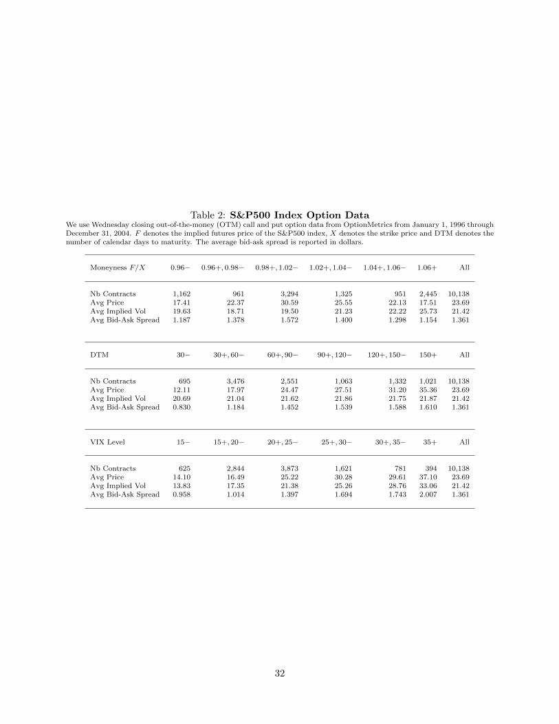
Table 2: S&P500 Index Option DataWe use Wednesday closing out-of-the-money (OTM) call and put option data from OptionMetrics from January 1, 1996 throughDecember 31, 2004. F denotes the implied futures price of the S&P500 index, X denotes the strike price and DTM denotes thenumber of calendar days to maturity. The average bid-ask spread is reported in dollars.
Moneyness F/X 0.96− 0.96+, 0.98− 0.98+, 1.02− 1.02+, 1.04− 1.04+, 1.06− 1.06+ All
Nb Contracts 1,162 961 3,294 1,325 951 2,445 10,138Avg Price 17.41 22.37 30.59 25.55 22.13 17.51 23.69Avg Implied Vol 19.63 18.71 19.50 21.23 22.22 25.73 21.42Avg Bid-Ask Spread 1.187 1.378 1.572 1.400 1.298 1.154 1.361
DTM 30− 30+, 60− 60+, 90− 90+, 120− 120+, 150− 150+ All
Nb Contracts 695 3,476 2,551 1,063 1,332 1,021 10,138Avg Price 12.11 17.97 24.47 27.51 31.20 35.36 23.69Avg Implied Vol 20.69 21.04 21.62 21.86 21.75 21.87 21.42Avg Bid-Ask Spread 0.830 1.184 1.452 1.539 1.588 1.610 1.361
VIX Level 15− 15+, 20− 20+, 25− 25+, 30− 30+, 35− 35+ All
Nb Contracts 625 2,844 3,873 1,621 781 394 10,138Avg Price 14.10 16.49 25.22 30.28 29.61 37.10 23.69Avg Implied Vol 13.83 17.35 21.38 25.26 28.76 33.06 21.42Avg Bid-Ask Spread 0.958 1.014 1.397 1.694 1.743 2.007 1.361
32

Table 3: Estimation Results on S&P500 Index Options: SVS and GARCH ModelsWe estimate the four SVS and the three GARCH models using option data for the period January 1, 1996 to December 31,2004. Standard errors, computed using the outer product of the gradient, are indicated in parentheses.
SVS Models
SVS1FC SVS1FU SVS2FC SVS2FU
Parameters Estimate Std Error Estimate Std Error Estimate Std Error Estimate Std Error
β1 -2.468E+3 (1.28E+2) -2.450E+3 (8.02E+1) -1.046E+4 (1.15E+3) -1.847E+4 (2.80E+3)η1 0.000E+0 -2.325E-1 (1.08E-2) 0.000E+0 1.083E-2 (3.92E-2)µ1 3.968E-5 (1.55E-6) 8.534E-5 (1.58E-6) 5.566E-6 (6.22E-7) 3.421E-6 (5.13E-7)φ1 9.879E-1 (2.13E-4) 9.920E-1 (1.59E-4) 9.763E-1 (5.83E-4) 9.770E-1 (7.75E-4)√ω1 2.315E-5 (8.98E-7) 2.684E-5 (4.96E-7) 3.616E-6 (3.88E-7) 2.097E-6 (3.08E-7)
β2 0.000E+0 -4.025E-1 (7.51E+1)η2 -1.975E-1 (5.88E-3) -2.018E-1 (5.82E-3)µ2 2.592E-5 (7.71E-6) 5.275E-5 (3.39E-6)φ2 9.989E-1 (1.60E-4) 9.982E-1 (1.35E-4)√ω2 6.672E-5 (4.42E-6) 5.275E-5 (1.49E-6)
Model Properties
Log Likelihood 20,100 21,080 21,851 21,880IVRMSE 3.557 3.156 2.981 2.970Ratio to HN 0.914 0.811 0.766 0.763
GARCH Models
HN CHJ CJOW
Parameters Estimate Std Error Estimate Std Error Estimate Std Error
µ1h 1.24E-4 (6.55E-7) 1.178E-4 (9.04E-7) 8.01E-5 (3.34E-6)φ1h 9.85E-1 (8.97E-5) 0.9857 (1.27E-4) 9.66E-1 (7.22E-4)α1h 1.81E-6 (5.85E-9) 1.68E-6 (2.04E-8) 2.44E-6 (1.39E-7)β1h 208.61 (4.62E+0) 238.50 (5.84E+0) 291.60 (1.60E+1)η1h -2.17E-3 (8.45E-5)
φ2h 9.97E-1 (1.49E-4)α2h 2.19E-6 (5.67E-8)β2h 2.22E+1 (2.13E+0)
Model Properties
Log Likelihood 19,158 19,277 21,623IVRMSE 3.890 3.783 3.000Ratio to HN 1.000 0.972 0.771
33
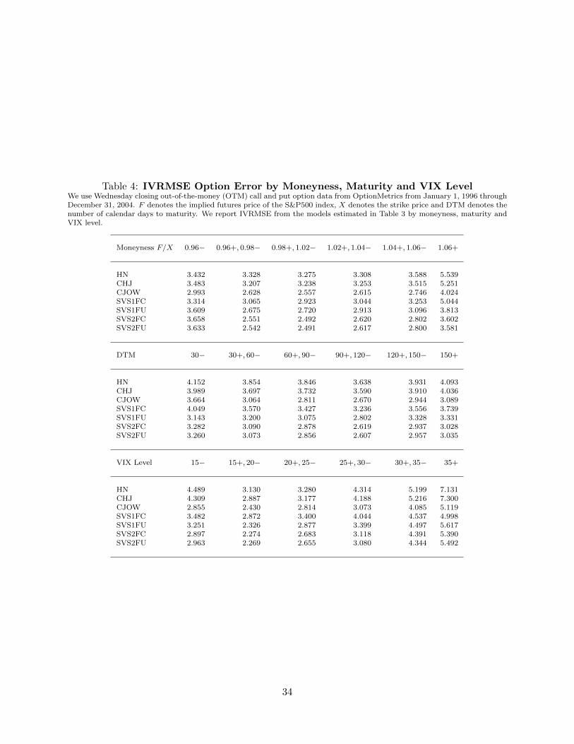
Table 4: IVRMSE Option Error by Moneyness, Maturity and VIX LevelWe use Wednesday closing out-of-the-money (OTM) call and put option data from OptionMetrics from January 1, 1996 throughDecember 31, 2004. F denotes the implied futures price of the S&P500 index, X denotes the strike price and DTM denotes thenumber of calendar days to maturity. We report IVRMSE from the models estimated in Table 3 by moneyness, maturity andVIX level.
Moneyness F/X 0.96− 0.96+, 0.98− 0.98+, 1.02− 1.02+, 1.04− 1.04+, 1.06− 1.06+
HN 3.432 3.328 3.275 3.308 3.588 5.539CHJ 3.483 3.207 3.238 3.253 3.515 5.251CJOW 2.993 2.628 2.557 2.615 2.746 4.024SVS1FC 3.314 3.065 2.923 3.044 3.253 5.044SVS1FU 3.609 2.675 2.720 2.913 3.096 3.813SVS2FC 3.658 2.551 2.492 2.620 2.802 3.602SVS2FU 3.633 2.542 2.491 2.617 2.800 3.581
DTM 30− 30+, 60− 60+, 90− 90+, 120− 120+, 150− 150+
HN 4.152 3.854 3.846 3.638 3.931 4.093CHJ 3.989 3.697 3.732 3.590 3.910 4.036CJOW 3.664 3.064 2.811 2.670 2.944 3.089SVS1FC 4.049 3.570 3.427 3.236 3.556 3.739SVS1FU 3.143 3.200 3.075 2.802 3.328 3.331SVS2FC 3.282 3.090 2.878 2.619 2.937 3.028SVS2FU 3.260 3.073 2.856 2.607 2.957 3.035
VIX Level 15− 15+, 20− 20+, 25− 25+, 30− 30+, 35− 35+
HN 4.489 3.130 3.280 4.314 5.199 7.131CHJ 4.309 2.887 3.177 4.188 5.216 7.300CJOW 2.855 2.430 2.814 3.073 4.085 5.119SVS1FC 3.482 2.872 3.400 4.044 4.537 4.998SVS1FU 3.251 2.326 2.877 3.399 4.497 5.617SVS2FC 2.897 2.274 2.683 3.118 4.391 5.390SVS2FU 2.963 2.269 2.655 3.080 4.344 5.492
34