a space-time discontinuous galerkin method for navier-stokes with
TRANSCRIPT
A Space-Time Discontinuous Galerkin Method forNavier-Stokes with Recovery
by
Kwok Ho Marcus Lo
A dissertation submitted in partial fulllmentof the requirements for the degree of
Doctor of Philosophy(Aerospace Engineering)
in The University of Michigan2011
Doctoral Committee:
Professor Bram van Leer, ChairProfessor Nikolaos D. KatopodesProfessor Philip L. RoeAssistant Professor Krzysztof J. FidkowskiHung T. Huynh, NASA Glenn

c© Kwok Ho Marcus Lo 2011
All Rights Reserved

ACKNOWLEDGEMENTS
I appreciate my loving mother, Katherine, for teaching me to rely on myself and
to stand tall. I thank my dad, Alan, for allowing me to pursue my love for science.
Thank you my brother, Michael, for taking care of me when I was almost dead on
the hospital bed. I am thankful for my wonderful pets, Miumiu and Momo, for
accompanying me through day and night, and through ups and downs. I am grateful
for Hung Huynh's enthusiasm and advice in CFD. Cheers to my research comrade,
Loc, for enduring my eccentricity. Lastly, I am innitely happy for this wonderful
life-learning experience with my friendly neighborhood professor, Bram van Leer and
his wife, Lia.
ii
PREFACE
Computational uid dynamics (CFD) is the branch of uid mechanics that uses
numerical methods and algorithms to solve uid problems. While there are currently
a myriad of numerical methods being used and developed, this dissertation focuses
on the Discontinuous Galerkin (DG) method because this method possesses superior
properties in regard to adapting to problem geometry, to parallelizing on today's
computer architecture, and to achieving super-convergence. Although DG works well
in hyperbolic problems where discontinuities frequently arise, the development in
parabolic problems, such as diusion, is lagging. The purpose of this dissertation is
to present a completely new concept, interface-centered recovery-based discontinuous
Galerkin (RDG) for diusion. Our goal is to develop a new diusion scheme that is
a quantum level better than existing methods; this includes higher-order of accuracy,
weaker time-stepping restriction, and easier understanding and implementation. We
begin by providing a historical overview of developments in DG for time-marching and
diusion schemes. The second chapter illustrates the generalized concept of recovery
in a mathematical framework. In next chapter, we present analysis and numerical
results in one dimension to facilitate understanding of the recovery concept. The
fourth chapter expands the recovery concept to two dimensions and unstructured
grids. We also include a new application of the recovery concept beyond diusion.
Recovery is used for enhancing the solution polynomial to a higher order; as a result
the recovery procedure uses more isotropic information resulting in a higher order of
accuracy. The choice of information is subject to optimization. The fth chapter pro-
vides numerical results for solving the Navier-Stokes viscous terms. The nal chapter
is the development of a new time-marching scheme for DG, moment method, not re-
stricted to diusion. The moment method was rst developed by Dr. Huynh (NASA
Glenn) for piecewise-linear solution representation. We present the implementation
and numerical results of higher-order moment schemes.
iii

TABLE OF CONTENTS
ACKNOWLEDGEMENTS . . . . . . . . . . . . . . . . . . . . . . . . . . ii
PREFACE . . . . . . . . . . . . . . . . . . . . . . . . . . . . . . . . . . . . . iii
LIST OF FIGURES . . . . . . . . . . . . . . . . . . . . . . . . . . . . . . . viii
LIST OF TABLES . . . . . . . . . . . . . . . . . . . . . . . . . . . . . . . . xv
LIST OF APPENDICES . . . . . . . . . . . . . . . . . . . . . . . . . . . . xx
CHAPTER
I. Introduction . . . . . . . . . . . . . . . . . . . . . . . . . . . . . . 1
1.1 Boris Grigoryevich Galerkin . . . . . . . . . . . . . . . . . . . 11.2 The discontinuous Galerkin method . . . . . . . . . . . . . . 21.3 History of advection and explicit time-marching methods for DG 6
1.3.1 The original DG: neutron transport . . . . . . . . . 71.3.2 Van Leer's schemes III & VI . . . . . . . . . . . . . 81.3.3 Runge-Kutta methods . . . . . . . . . . . . . . . . . 81.3.4 ADER and STE-DG methods . . . . . . . . . . . . 91.3.5 Huynh's upwind moment method . . . . . . . . . . 101.3.6 Hancock discontinuous Galerkin method . . . . . . 11
1.4 History of diusion methods for DG . . . . . . . . . . . . . . 111.4.1 The (σ, µ)-family . . . . . . . . . . . . . . . . . . . 121.4.2 Approaches based on a system of rst-order equa-
tions . . . . . . . . . . . . . . . . . . . . . . . . . . 131.4.3 Recovery-based discontinuous Galerkin method . . . 151.4.4 Flux-based diusion approach . . . . . . . . . . . . 151.4.5 Huynh's reconstruction approach . . . . . . . . . . . 161.4.6 Combining DG advection with DG diusion . . . . 17
1.5 Motivation . . . . . . . . . . . . . . . . . . . . . . . . . . . . 181.6 Outline of this thesis: the River of Recovery . . . . . . . . . . 19
II. Interface-centered Recovery-based Method for Diusion . . . 21
iv

2.1 The beginning of RDG . . . . . . . . . . . . . . . . . . . . . 212.2 Cartoon illustration of recovery in 1-D . . . . . . . . . . . . . 232.3 Interface recovery equations . . . . . . . . . . . . . . . . . . . 24
2.3.1 Full-rank Rj,j+1 . . . . . . . . . . . . . . . . . . . . 262.3.2 Reducing the condition number of Rj,j+1 . . . . . . 27
2.4 Smooth recovery polynomial basis . . . . . . . . . . . . . . . 302.5 Interface-centered recovery-based discontinuous Galerkin (iRDG)
Method . . . . . . . . . . . . . . . . . . . . . . . . . . . . . . 322.6 Evolution of the recovery-based discontinuous
Galerkin methods . . . . . . . . . . . . . . . . . . . . . . . . 342.7 Stability proofs for interface recovery-based discontinuous Galerkin
methods . . . . . . . . . . . . . . . . . . . . . . . . . . . . . . 352.7.1 Proof for RDG-2x . . . . . . . . . . . . . . . . . . . 352.7.2 Proof for RDG-1x-Naive . . . . . . . . . . . . . . . 382.7.3 Note on RDG-1x-Smart . . . . . . . . . . . . . . . . 38
2.8 Recovery concept for solution enhancement . . . . . . . . . . 39
III. RDG in One-Dimension for Scalar Equation . . . . . . . . . . 40
3.1 1-D recovery equations for binary recovery . . . . . . . . . . . 413.1.1 Piecewise-constant (p = 0) recovery . . . . . . . . . 413.1.2 Piecewise-linear (p = 1) recovery . . . . . . . . . . . 423.1.3 Piecewise-quadratic (p = 2) recovery . . . . . . . . . 43
3.2 RDG-2x for linear diusion . . . . . . . . . . . . . . . . . . . 443.3 Fourier analysis and eigenvectors . . . . . . . . . . . . . . . . 47
3.3.1 RDG-2x Fourier analysis: piecewise-linear (p = 1) . 483.3.2 RDG-2x Fourier analysis: piecewise-quadratic (p =
2) . . . . . . . . . . . . . . . . . . . . . . . . . . . 543.3.3 The venerable (σ, µ)-family Fourier analysis for p = 1 563.3.4 The new (σ, µ, ω)-family for p = 1 . . . . . . . . . . 693.3.5 Bilinear form of RDG . . . . . . . . . . . . . . . . . 70
3.4 Numerical results for the original RDG-2x . . . . . . . . . . 713.4.1 Recovery at the domain boundary . . . . . . . . . . 713.4.2 Linear diusion . . . . . . . . . . . . . . . . . . . . 743.4.3 Linear advection-diusion . . . . . . . . . . . . . . . 79
3.5 RDG schemes for variable diusion coecient . . . . . . . . . 853.5.1 RDG-1x+ with recovery concept for solution enhance-
ment . . . . . . . . . . . . . . . . . . . . . . . . . . 883.5.2 Fourier analysis of various RDG schemes . . . . . . 933.5.3 Linear variation of diusion coecient . . . . . . . . 933.5.4 Nonlinear variation of diusion coecient . . . . . 95
3.6 Chapter summary . . . . . . . . . . . . . . . . . . . . . . . . 97
IV. RDG in Two-Dimensions for a Scalar Equation . . . . . . . . 100
v
4.1 2-D recovery equations for binary recovery . . . . . . . . . . . 1004.1.1 Transformation from global to local coordinate . . . 1014.1.2 Tranformation from global to recovery coordinates . 1034.1.3 Orthogonal basis functions . . . . . . . . . . . . . . 1044.1.4 Recovery basis derived from tensor product basis . . 106
4.2 RDG Schemes for 2-D . . . . . . . . . . . . . . . . . . . . . . 1074.2.1 Recovery at the domain boundary . . . . . . . . . . 1074.2.2 Linear RDG schemes . . . . . . . . . . . . . . . . . 1104.2.3 Nonlinearity and cross-derivatives in RDG schemes . 118
4.3 Chapter summary . . . . . . . . . . . . . . . . . . . . . . . . 127
V. Navier-Stokes Equations with RDG . . . . . . . . . . . . . . . . 129
5.1 1-D Navier-Stokes Equations with RDG . . . . . . . . . . . . 1295.1.1 Discretization of 1-D Navier-Stokes viscous terms . 131
5.2 2-D Navier-Stokes . . . . . . . . . . . . . . . . . . . . . . . . 1365.2.1 2-D Navier-Stokes Viscous Terms . . . . . . . . . . 138
5.3 Chapter summary . . . . . . . . . . . . . . . . . . . . . . . . 141
VI. Hancock-Huynh Discontinuous Galerkin Method . . . . . . . 142
6.1 Hancock's Observation . . . . . . . . . . . . . . . . . . . . . . 1446.2 Space-time discontinuous Galerkin discretization for advection 146
6.2.1 One-dimension linear advection . . . . . . . . . . . 1476.2.2 One-dimensional Euler equations . . . . . . . . . . 1576.2.3 Summary of HH-DG for advection . . . . . . . . . . 165
6.3 Space-time discontinuous Galerkin for diusion . . . . . . . . 1666.3.1 Deriving space-time diusion schemes . . . . . . . . 1676.3.2 Hancock-Huynh interface-centered recovery-based dis-
continuous Galerkin method (HH-RDG) . . . . . . . 1856.4 HH-DG linear advection-diusion in 1-D . . . . . . . . . . . . 192
6.4.1 Piecewise-linear & piecewise-quadratic HH-DG forlinear advection-diusion equation . . . . . . . . . . 195
6.4.2 Numerical results for linear advection-diusion withHH-DG . . . . . . . . . . . . . . . . . . . . . . . . . 198
6.4.3 Fourier analysis of HH-DG for linear advection diusion1996.5 Chapter summary . . . . . . . . . . . . . . . . . . . . . . . . 202
VII. Conclusions . . . . . . . . . . . . . . . . . . . . . . . . . . . . . . . 204
7.1 Summary . . . . . . . . . . . . . . . . . . . . . . . . . . . . . 2047.2 Future work . . . . . . . . . . . . . . . . . . . . . . . . . . . 2077.3 The eort: revisiting the River of Recovery . . . . . . . . . . 209
vi

APPENDICES . . . . . . . . . . . . . . . . . . . . . . . . . . . . . . . . . . 211
BIBLIOGRAPHY . . . . . . . . . . . . . . . . . . . . . . . . . . . . . . . . 232
vii

LIST OF FIGURES
Figure
1.1 Boris Grigoryevich Galerkin . . . . . . . . . . . . . . . . . . . . . . 2
1.2 Continuous Galerkin (left) and discontinuous Galerkin (right) solu-tion representations showing the key dierence is the requirement ofcontinuity across element interface . . . . . . . . . . . . . . . . . . 5
1.3 Interpretation of BR1 (left) and BR2 (right) for scalar 1-D diusion.Two new local solutions are reconstructed on the left and right ofthe indicated interface as gL and gR respectively. The large solid dotindicates the average of the left and right values at the interface. Theschemes also adopt the average of the derivative values as the interfacevalue of ux. Notice BR1 utilizes a 4-cell stencil for an interface ux,while the newer BR2 utilizes a 2-cell stencil. . . . . . . . . . . . . . 14
1.4 Interpretation of two versions of LDG for scalar 1-D diusion. Twonew local solutions are reconstructed on the left and right of theindicated interface as gL and gR respectively. The large solid dotindicates the common function value. The LDG is a non-symmetricscheme using the function value of gL for u, but the derivative valueof gR for ux, (left) or vice versa (right). . . . . . . . . . . . . . . . . 14
1.5 The outline of this thesis is represented by the River of Recovery. . 20
2.1 Finite-element analyst answering nite-volume analyst regarding DGfor diusion. Courtesy of Van Leer, 2005. . . . . . . . . . . . . . . 22
2.2 The essence of recovery. Start with the exact solution U on the left(dashed line). The discretized solution u in the middle is piecewiselinear (thick solid line). We recover a smooth function f (right, thinsolid line). . . . . . . . . . . . . . . . . . . . . . . . . . . . . . . . . 23
viii

2.3 A little block game for determining the recovery basis in 1-D. Theblocks on the left and right of the dashed line indicate basis functionsof the solution in Ωj and Ωj+1 respectively. Now imagine gravity pullsto the left; the blocks from Ωj+1 fall on top of the blocks in Ωj toform the recovery basis. . . . . . . . . . . . . . . . . . . . . . . . . . 26
2.4 A little block game for determining the recovery basis in 2-D. Theblocks on the left and right of the dashed line indicate basis functionof the solution in Ωj and Ωj+1 respectively. Now imagine gravitypulls to the left; the blocks from Ωj+1 fall on top of the blocks inΩj to form the recovery basis. Notice there are more blocks in ther-coordinate than in the s-coordinate. . . . . . . . . . . . . . . . . . 27
2.5 In the p = 0 case, there is a total of two SRB functions. The smoothrecovery basis functions (solid lines) replacing vj = 1 (dashed lines)in Ωj (left), and vj+1 = 1 in Ωj+1 (right). . . . . . . . . . . . . . . . 31
2.6 In the p = 1 case, there is a total of four SRB functions. The smoothrecovery basis functions (solid lines) replacing vj = 1 and vj = 2ξ− 1(dashed lines) in Ωj (left), and vj+1 = 1 and vj+1 = 2ξ − 1 in Ωj+1
(right). . . . . . . . . . . . . . . . . . . . . . . . . . . . . . . . . . . 31
3.1 The recovery coordinate system spans the union of two neighboringcells, while each cell has a local coordinate ξ. . . . . . . . . . . . . 42
3.2 Eigenvalues of RDG-2x (p = 1) are shown on the left. The switchfunctions are shown on the right demonstrating the contribution ofeach eigenfunction for various β. . . . . . . . . . . . . . . . . . . . 50
3.3 Eigenfunctions of RDG-2x (p = 1) for β between π5and 99π
100. Notice
the change in scaling of both x-axis and g-axis. The dashed linerepresents the analytical wave. . . . . . . . . . . . . . . . . . . . . 52
3.4 Eigenfunctions of RDG-2x (p = 1) for β for 4π3and 5π
3. Notice the
change in scaling of both x-axis and g-axis. The dashed line repre-sents the analytical wave. . . . . . . . . . . . . . . . . . . . . . . . 53
3.5 Eigenvalues of RDG-2x (p = 2), are shown on the left. The switchfunctions are shown on the right demonstrating the contribution ofeach eigenfunction for various β. . . . . . . . . . . . . . . . . . . . 55
3.6 A closer look at the good eigenvalue of RDG-2x (p = 2), for small β.The dierence between the good eigenvalue and the exact diusionoperator is of order β10, implying the evolution error of the schemeis 8th-order. . . . . . . . . . . . . . . . . . . . . . . . . . . . . . . . 55
ix
3.7 Eigenfunctions of RDG-2x (p = 2) for β between π5and 5π
3. Notice
the change in scaling of both x-axis and g-axis. The dashed linerepresents the analytical wave. . . . . . . . . . . . . . . . . . . . . . 57
3.8 For small β, C1 and C2 are the weighting coecients of the badeigenvectors. They scale with β8. However, no solid conclusion canbe drawn from this analysis due to the lack of analytical formulas. . 58
3.9 A intuitive map of the (σ, µ)-family. The symbols are dened asfollow: S is the symmetric scheme, SA is the symmetric/Arnoldscheme, I is the inconsistent scheme, BR2 is Bassi-Rebay 2. Thedark region indicates instability, the light gray region represents ef-cient and stable schemes with the largest Von Neumann number(VNN), and the white region designates the stable domain. . . . . . 61
3.10 Stencils of full boundary-recovered function (left) and compact boundary-recovered function (right). The thick solid line indicates the domainboundary, and B.C. stands for boundary condition, which can beDirichlet or Neumann. . . . . . . . . . . . . . . . . . . . . . . . . . 73
3.11 Upwind-RDG-2x (p = 1) Péclet number study. Numbers indicate theorder of accuracy in the L2-norm. The left axis indicates the valueof PeG, while the dotted lines indicate contours of constant PeL. Weobserve the order of accuracy of upwind-RDG-2x decreases in theupper right corner where the advection physics dominate, reectingthe order of accuracy of the DG upwind scheme only. . . . . . . . . 85
3.12 Upwind-RDG-2x (p = 2) Péclet number study. Numbers indicate theorder of accuracy in the L2-norm. Unfortunately, the rates are notreliable because the diusion scheme is too accurate and the errorsare at the computer-zero level. We are still able to observe that nearthe top right region where the advection physics dominate, the rateis dominated by the upwind scheme. . . . . . . . . . . . . . . . . . 86
3.13 Recovery concept is used for both diusion ux and solution en-hancement. BR stands for binary recovery; SE stands for solutionenhancement. The cycle of BR followed by SE can be repeated overand over again until the desired level of enhancement is achieved. . 90
4.1 Mapping from the global coordinates to the local coordinates. Thearbitrary triangle T is transformed into a standard triangle TS. Thearbitrary quadrilateral Q is transformed into a standard square QS. 101
4.2 Mapping from global to recovery coordinates. . . . . . . . . . . . . 104
x

4.3 A little block game for determining the recovery basis in 2-D. Theblocks on the left and right of the dotted line indicate basis functionsof the solution in Ωj and Ωj+1 respectively. Now imagine gravitypulls to the left; the blocks from Ωj+1 fall on top of the blocks inΩj to form the recovery basis. Notice there are more blocks in ther-coordinate than in the s-coordinate. . . . . . . . . . . . . . . . . . 106
4.4 Full boundary-recovered functions for 2-D Cartesian grid for p = 1on the left and p = 2 on the right. The domain boundary providesp+ 1 conditions based on the Dirichlet function, g. Notice the choiceof moments to satisfy in Ω2 is not arbitrary. . . . . . . . . . . . . . 108
4.5 (Left) The hollow circles indicate the centroids of the triangles. It isdicult to obtain a full boundary-recovered function due to the align-ment of cell centers that is more biased in the face-parallel direction.(Right) Compact boundary-recovered function for 2-D Cartesian gridfor p = 1. The domain boundary provides p+ 1 conditions based onthe Dirichlet boundary condition, g (x, y). . . . . . . . . . . . . . . 109
4.6 Experiment 1, RDG-2x (p = 1) for time-accurate problem with peri-odic boundary conditions. The order of error convergence is 4th-orderfor the cell average, and 5th-order for the averaged rst gradient. . . 113
4.7 Experiment 1, RDG-2x (p = 2) for time-accurate problem with peri-odic boundary conditions. The order of error convergence is 8th-orderfor the cell average, and 7th-order for the averaged rst gradient. . . 113
4.8 Experiment 1, RDG-2x (p = 3) for time-accurate problem with pe-riodic boundary conditions. The order of error convergence is 10th-order for the cell average, and 11th-order for the averaged rst gra-dient. The dip for the course grid is due to the average rst gradientbeing zero on a 2 by 2 grid. . . . . . . . . . . . . . . . . . . . . . . 114
4.9 Experiment 2. Left: RDG-2x (p = 1) for steady-state problem usingfull boundary-recovered function at the Dirichlet boundaries. Right:Comparison of various RDG (p = 1) schemes with full boundary-recovered function. . . . . . . . . . . . . . . . . . . . . . . . . . . . 116
4.10 Experiment 3, RDG-2x (p = 1, 2, 3, 4) for steady-state problem usingcompact boundary-recovered function at the Dirichlet boundaries. Asample perturbed grid is shown on the left, and the graph on theright shows the order of accuracy of the scheme to be p + 1 on theirregular triangular grid. . . . . . . . . . . . . . . . . . . . . . . . . 117
xi

4.11 Experiment 3, RDG-2x and RDG-1x-Naive (p = 1, 2, 3) for steady-state problem using a compact boundary-recovered function at theDirichlet boundaries. It appears that RDG-2x is only slightly betterthan RDG-1x on a triangular grid. . . . . . . . . . . . . . . . . . . . 117
4.12 Basis functions for u in 2-D Cartesian grid for p = 0, 1, and 2 fromleft to right. . . . . . . . . . . . . . . . . . . . . . . . . . . . . . . . 119
4.13 The recovered function is inaccurate in the face-tangential direction.We apply binary recovery on top of u to get an enhanced recoveredfunction f to improve on the accuracy of f in the face-tangentialdirections. . . . . . . . . . . . . . . . . . . . . . . . . . . . . . . . . 121
4.14 The 2-D stencils for various RDG schemes. Stencil size has directinuence on the time-step of explicit time-marching schemes, andalso on the matrix density of implicit time-marching schemes. . . . . 122
4.15 The stencils of the enhanced recovered function for RDG-1x++ andRDG-1x++CO on the left and right, respectively. . . . . . . . . . . 122
4.16 Reduced-accuracy y-recovery, followed by standard x-recovery, to cre-ate an enhanced recovered function f for use at an interface alongthe y-direction. . . . . . . . . . . . . . . . . . . . . . . . . . . . . . 123
4.17 Experiment 5, RDG-1x++ and RDG-1x++CO (p = 1) for time-accurateproblem with periodic boundary conditions. The order of error con-vergence is 4 for the cell average, and 5 for the averaged rst gradient.124
4.18 Experiment 5, RDG-1x++ and RDG-1x++CO (p = 2) for time-accurateproblem with periodic boundary conditions. Notice the Cartesian op-timized version performs extremely well. . . . . . . . . . . . . . . . 125
4.19 Experiment 5, RDG-1x++ and RDG-1x++CO (p = 3) for time-accurateproblem with periodic boundary conditions. The order of error con-vergence is 10 for the cell average, and 9 for the averaged rst gradient.125
6.1 Hancock observes that the waves generated from the local evolutionof two elements, Ωj and Ωj+1, result in the correct waves arriving atthe element interface centered on xj+ 1
2. . . . . . . . . . . . . . . . . 145
6.2 The exact shift operator occurs when ν = 1. The solution of Ωj att = t0 + ∆t is equal to the solution of Ωj−1 at t = t0. . . . . . . . . . 149
xii

6.3 For ν < 1, the subcell shift causes the original discontinuity at theinterface to be shifted to the interior of Ωj. The new solution of Ωj
(dotted line) is now acquired by projecting the discontinuous solutionushiftedj into the solution space. . . . . . . . . . . . . . . . . . . . . 149
6.4 HH-DG (p = 2) using local Runge-Kutta to obtain ust. Dashedlines indicates location of stored space-time solution values. Thelightly dotted lines are characteristics from Ωj and they illustrate animportant property of locality. For LRK, these characteristics areassumed to be valid outside of Ωj, hence the function values of u onthe boundaries are uniquely dened. . . . . . . . . . . . . . . . . . 152
6.5 At the interface between two space-time expanded solutions (repre-sented by solid dots), an approximate Riemann solver (indicated byellipses) is applied at the Radau points to acquire unique ux valuesat each time level. . . . . . . . . . . . . . . . . . . . . . . . . . . . . 153
6.6 Amplication factor of the 4th-order diusion scheme using centraldierencing. A maximum of r = 0.66 is achieved with regard tostability. . . . . . . . . . . . . . . . . . . . . . . . . . . . . . . . . . 170
6.7 Amplication factor of the 6th-order diusion scheme using centraldierencing. A maximum of r = 0.84 is achieved. . . . . . . . . . . 172
6.8 The two amplication factors associated with a nite-dierence schemewith p = 1 subgrid information. The resulting scheme is 4th-orderaccurate in time. Notice for r = 1
12, the two amplication factors are
distinct, while for r = 16, the two amplication factors coincide with
each other. . . . . . . . . . . . . . . . . . . . . . . . . . . . . . . . . 174
6.9 The three amplication factors associated with the FD scheme withp = 2 subgrid information is shown for r = 0.0529 (left) and r = 0.124(right). The eigenvalues are real up to r = 0.0529. The eigenvaluesbecome complex for r ≥ 0.0529 and the amplication factors remainunder unity up till r = 0.124. . . . . . . . . . . . . . . . . . . . . . . 177
6.10 Polar plots in the complex plane of the two eigenvalues of the updatematrix of HH-RDG (p = 1) scheme. The dashed line indicates thestability boundary. For r = 1
6, the two eigenvalues coincide. For
anything larger than r = 16, one eigenvalue lies outside of the stability
domain. . . . . . . . . . . . . . . . . . . . . . . . . . . . . . . . . . 191
xiii
6.11 Polar plots in the complex plane of the two eigenvalues of the updatematrix of HH-RDG (p = 2) scheme. The dashed line indicates thestability boundary. For r = 1
10, the three eigenvalues remain bounded
by the stability circle. For r larger than 110, one eigenvalue lies outside
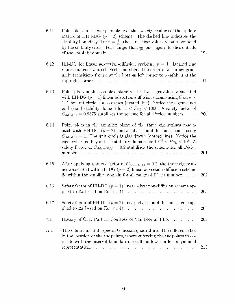
of the stability domain. . . . . . . . . . . . . . . . . . . . . . . . . . 192
6.12 HH-DG for linear advection-diusion problem, p = 1. Dashed linerepresents constant cell Péclet number. The order of accuracy grad-ually transitions from 4 at the bottom left corner to roughly 3 at thetop right corner. . . . . . . . . . . . . . . . . . . . . . . . . . . . . . 199
6.13 Polar plots in the complex plane of the two eigenvalues associatedwith HH-DG (p = 1) linear advection-diusion scheme using CAdv-Di =1. The unit circle is also drawn (dotted line). Notice the eigenvaluesgo beyond stability domain for 1 < PeL < 1000. A safety factor ofCAdv-Di = 0.9375 stabilizes the scheme for all Péclet numbers. . . . 200
6.14 Polar plots in the complex plane of the three eigenvalues associ-ated with HH-DG (p = 2) linear advection-diusion scheme usingCAdv-Di = 1. The unit circle is also drawn (dotted line). Notice theeigenvalues go beyond the stability domain for 10−3 < PeL < 108. Asafety factor of CAdv−Diff = 0.2 stabilizes the scheme for all Pécletnumbers. . . . . . . . . . . . . . . . . . . . . . . . . . . . . . . . . . 201
6.15 After applying a safety factor of CAdv−Diff = 0.2, the three eigenval-ues associated with HH-DG (p = 2) linear advection-diusion schemelie within the stability domain for all range of Péclet number. . . . . 202
6.16 Safety factor of HH-DG (p = 1) linear advection-diusion scheme ap-plied to ∆t based on Eqn 6.144 . . . . . . . . . . . . . . . . . . . . 203
6.17 Safety factor of HH-DG (p = 2) linear advection-diusion scheme ap-plied to ∆t based on Eqn 6.144 . . . . . . . . . . . . . . . . . . . . 203
7.1 History of CFD Part II: Courtesy of Van Leer and Lo. . . . . . . . . 208
A.1 Three fundamental types of Gaussian quadrature. The dierence liesin the location of the endpoints, where enforcing the endpoints to co-incide with the interval boundaries results in lower-order polynomialrepresentation. . . . . . . . . . . . . . . . . . . . . . . . . . . . . . . 213
xiv

LIST OF TABLES
Table
2.1 Condition number of Rj,j+1 for recovery between two right triangu-lar elements with p = 1 solutions. Notice quadrilateral Legendrepolynomials (Q. Legendre) are no longer orthogonal on a triangle do-main. Each face of the triangle has a dierent condition number; themaximum condition number of the three is reported. . . . . . . . . . 30
3.1 Numerical Fourier analysis of RDG-1xf show the scheme to be unsta-ble for p ≥ 3 due to positive eigenvalues. RDG-1xf is an experimentalscheme. . . . . . . . . . . . . . . . . . . . . . . . . . . . . . . . . . . 66
3.2 Stability range and order of error convergence of various schemesof the (σ, µ)-family. The maximum stable Von Neumann number(VNN) is found numerically to the nearest one-hundredths, and theCPU time for numerical convergence is given in seconds. The * sym-bol indicates schemes lying on the thick solid line of the (σ, µ)-map. 68
3.3 Coecients of the penalty-like terms in 1-D RDG-2x for p ≤ 5. . . . 70
3.4 L2-error of RDG-2x scheme for steady-state problem with periodicboundary condition. * stands for undetermined order of accuracy.The extremely high accuracy of the cell average of the p = 2 scheme,and both cell average and rst gradient of the p = 3 scheme arereferred to as innite accuracy. . . . . . . . . . . . . . . . . . . . . 76
3.5 L2-error of RDG-2x scheme for time-accurate problem with periodicboundary condition. . . . . . . . . . . . . . . . . . . . . . . . . . . 78
3.6 L2-error of RDG-2x scheme for steady-state problem with mixedboundary condition using full boundary-recovered function. . . . . 80
3.7 L2-error of RDG-2x scheme for steady-state problem with mixedboundary condition using compact boundary-recovered function. . 81
xv

3.8 Flops comparison between RDG and cRDG for solution enhancementon a Cartesian grid, where (NRDG, NcRDG) is (2, 3), (5, 9), and (6, 27)for 1-D, 2-D, and 3-D, respectively. RDG in 2-D and 3-D is more thanan order of magnitude cheaper than cRDG. . . . . . . . . . . . . . . 89
3.9 Rate of L2-error convergence. The VNN number are given for RK3,RK4 and RK5 for p = 1, 2, and 3, respectively. . . . . . . . . . . . . 93
3.10 Convergence rate of L2-error. The VNN number are given for RK3,RK4 and RK5 for p = 1, 2, and 3, respectively. . . . . . . . . . . . . 95
3.11 L2-error of RDG-1x+ scheme for steady-state nonlinear diusionproblem with periodic boundary condition. . . . . . . . . . . . . . . 98
4.1 Tensor-product basis for Legendre polynomials. . . . . . . . . . . . 105
4.2 A sample orthonormal basis (p = 4) for the standard triangle. . . . 106
4.3 Experiment 4, L2-error of the cell average for the RDG-1x+ andRDG-0x+ schemes. . . . . . . . . . . . . . . . . . . . . . . . . . . 120
4.4 Fourier-analysis results for α = 0 (pure Laplacian). Note that RDG-1x+, RDG-1x++CO, and RDG-2x are identical. . . . . . . . . . . 126
4.5 Fourier analysis results for α = 1 (with cross-derivative). The maxi-mum real eigenvalue of RDG-1x++CO is about half of that of RDG-1x++. . . . . . . . . . . . . . . . . . . . . . . . . . . . . . . . . . . 127
5.1 p = 1 results for RDG-1x-Naive, 1xf , and 1x+. RDG-1x+ is clearlythe fastest scheme, while its accuracy is on par with RDG-1xf . . . 135
5.2 p = 2 results for RDG-1x-Naive, 1xf , and 1x+. RDG-1x+ is clearlythe fastest and most accurate scheme. . . . . . . . . . . . . . . . . 136
5.3 L2-error of the cell average of total energy for the RDG-1x++ andRDG-1x++CO schemes. . . . . . . . . . . . . . . . . . . . . . . . . 141
6.1 A comparison of order of accuracy between STE-DG and HH-DG forp = 1, tfinal = 3. HH-DG is roughly 3 times faster than STE-DG,and is one order higher in terms of accuracy of the cell average. . . 157
6.2 Order of accuracy for p = 1, 2, 3, CFL = 0.9375, tfinal = 300. . . . . 158
xvi
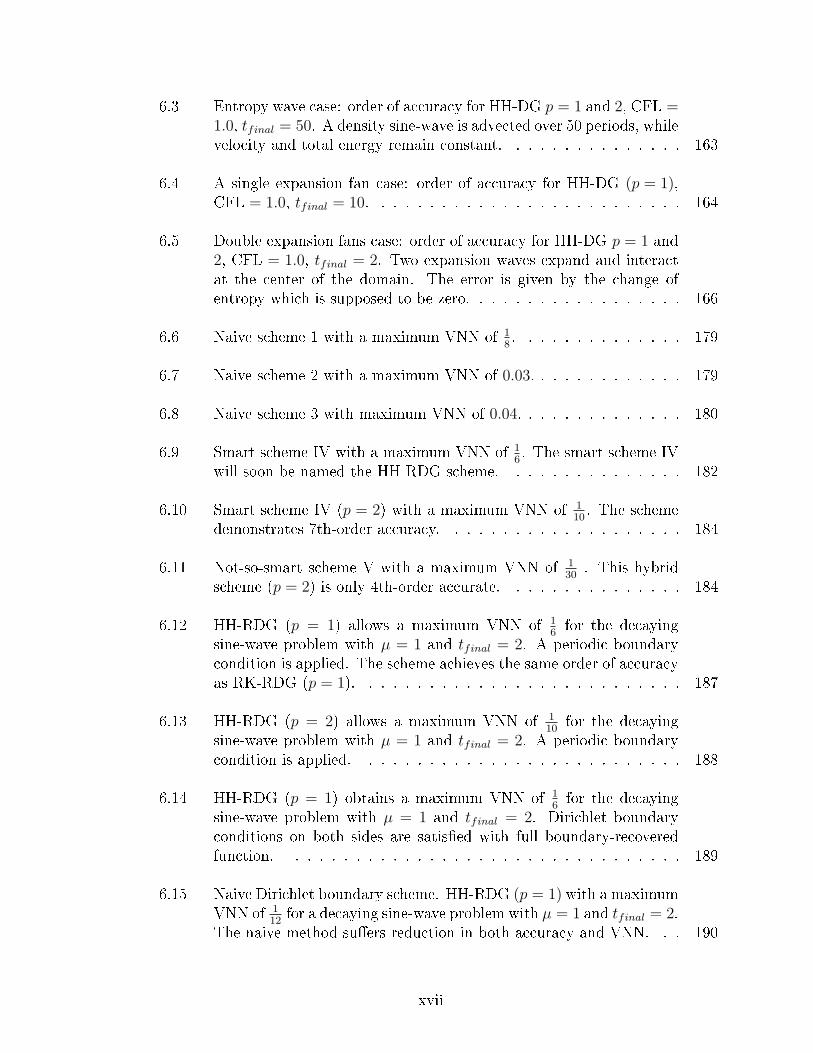
6.3 Entropy wave case: order of accuracy for HH-DG p = 1 and 2, CFL =1.0, tfinal = 50. A density sine-wave is advected over 50 periods, whilevelocity and total energy remain constant. . . . . . . . . . . . . . . 163
6.4 A single expansion fan case: order of accuracy for HH-DG (p = 1),CFL = 1.0, tfinal = 10. . . . . . . . . . . . . . . . . . . . . . . . . . 164
6.5 Double expansion fans case: order of accuracy for HH-DG p = 1 and2, CFL = 1.0, tfinal = 2. Two expansion waves expand and interactat the center of the domain. The error is given by the change ofentropy which is supposed to be zero. . . . . . . . . . . . . . . . . . 166
6.6 Naive scheme 1 with a maximum VNN of 18. . . . . . . . . . . . . . 179
6.7 Naive scheme 2 with a maximum VNN of 0.03. . . . . . . . . . . . . 179
6.8 Naive scheme 3 with maximum VNN of 0.04. . . . . . . . . . . . . . 180
6.9 Smart scheme IV with a maximum VNN of 16. The smart scheme IV
will soon be named the HH-RDG scheme. . . . . . . . . . . . . . . 182
6.10 Smart scheme IV (p = 2) with a maximum VNN of 110. The scheme
demonstrates 7th-order accuracy. . . . . . . . . . . . . . . . . . . . 184
6.11 Not-so-smart scheme V with a maximum VNN of 130
. This hybridscheme (p = 2) is only 4th-order accurate. . . . . . . . . . . . . . . 184
6.12 HH-RDG (p = 1) allows a maximum VNN of 16for the decaying
sine-wave problem with µ = 1 and tfinal = 2. A periodic boundarycondition is applied. The scheme achieves the same order of accuracyas RK-RDG (p = 1). . . . . . . . . . . . . . . . . . . . . . . . . . . 187
6.13 HH-RDG (p = 2) allows a maximum VNN of 110
for the decayingsine-wave problem with µ = 1 and tfinal = 2. A periodic boundarycondition is applied. . . . . . . . . . . . . . . . . . . . . . . . . . . 188
6.14 HH-RDG (p = 1) obtains a maximum VNN of 16for the decaying
sine-wave problem with µ = 1 and tfinal = 2. Dirichlet boundaryconditions on both sides are satised with full boundary-recoveredfunction. . . . . . . . . . . . . . . . . . . . . . . . . . . . . . . . . 189
6.15 Naive Dirichlet boundary scheme. HH-RDG (p = 1) with a maximumVNN of 1
12for a decaying sine-wave problem with µ = 1 and tfinal = 2.
The naive method suers reduction in both accuracy and VNN. . . 190
xvii

A.1 Sample classical Gaussian quadrature points and weights for the in-terval x ∈ [0, 1]. . . . . . . . . . . . . . . . . . . . . . . . . . . . . . 213
A.2 Sample Gauss-Radau quadrature points and weights for the intervalx ∈ [0, 1]. . . . . . . . . . . . . . . . . . . . . . . . . . . . . . . . . . 214
A.3 Initial projection error eL2,proj of three dierent (σ, µ)-schemes at t =0. . . . . . . . . . . . . . . . . . . . . . . . . . . . . . . . . . . . . 216
A.4 Evolution error eL2,evol with v = 1 of three dierent (σ, µ)-schemes att =∞. . . . . . . . . . . . . . . . . . . . . . . . . . . . . . . . . . 216
A.5 Final projection error eL2,proj of three dierent (σ, µ)-schemes at t =∞.217
A.6 Implicit Radau integration weights for n = 2 and 3. . . . . . . . . . 219
B.1 Linear diusion: L2-error of various σ − µ schemes (p = 1). . . . . . 221
B.2 Linear diusion: L2-error of various σ − µ schemes (p = 1). . . . . . 222
B.3 L2-error of RK-Upwind-DG scheme for time-accurate problem withperiodic boundary condition. A sine wave is advected to the right for100 cycles. . . . . . . . . . . . . . . . . . . . . . . . . . . . . . . . . 223
B.4 Linear advection-diusion: RK-Upwind-RDG-2x, p = 1, r = 16,
CFL = 0.4, µ = 0.01, tfinal = 100, periodic boundary condition. . . 224
B.5 Linear advection-diusion: RK-Upwind-RDG-2x, p = 1, r = 16,
CFL = 0.4, µ = 0.01, tfinal = 100, periodic boundary condition. . . 225
B.6 Linear advection-diusion: RK-Upwind-RDG-2x, p = 2, r = 110,
CFL = 0.27, µ = 0.01, tfinal = 100, periodic boundary condition. . 225
B.7 RDG-1x-Naive, VNN = 0.07, 0.02, and 0.01 for RK3, RK4, andRK5, respectively: L2-error of steady linear-variation diusion prob-lem with two-sided Neumann boundary conditions. . . . . . . . . . 226
B.8 RDG-2x, VNN = 0.15, 0.08, and 0.04 for RK3, RK4, and RK5, re-spectively: L2-error of steady linear-variation diusion problem withtwo-sided Neumann boundary conditions. . . . . . . . . . . . . . . . 227
B.9 RDG-1xf , VNN = 0.08, 0.02, and 0.0001 for RK3, RK4, and RK5, re-spectively: L2-error of steady linear-variation diusion problem withtwo-sided Neumann boundary conditions. . . . . . . . . . . . . . . . 228
xviii
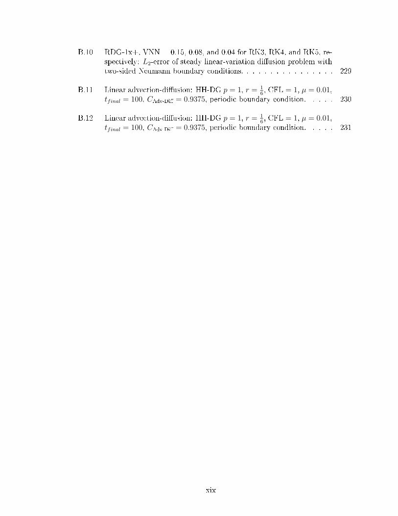
B.10 RDG-1x+, VNN = 0.15, 0.08, and 0.04 for RK3, RK4, and RK5, re-spectively: L2-error of steady linear-variation diusion problem withtwo-sided Neumann boundary conditions. . . . . . . . . . . . . . . . 229
B.11 Linear advection-diusion: HH-DG p = 1, r = 16, CFL = 1, µ = 0.01,
tfinal = 100, CAdv-Di = 0.9375, periodic boundary condition. . . . . 230
B.12 Linear advection-diusion: HH-DG p = 1, r = 16, CFL = 1, µ = 0.01,
tfinal = 100, CAdv-Di = 0.9375, periodic boundary condition. . . . . 231
xix
LIST OF APPENDICES
Appendix
A. Elements of Computational Fluid Dynamics . . . . . . . . . . . . . . . 212
B. Graveyard of Numbers . . . . . . . . . . . . . . . . . . . . . . . . . . 220
xx

CHAPTER I
Introduction
We introduce two new methods into the discontinuous Galerkin (DG) framework.
The rst is the recovery-based discontinuous Galerkin (RDG) method for diusion,
and the second is the Hancock-Huynh discontinuous Galerkin (HH-DG) method as
a space-time method. This dissertation details the progress and challenges we have
encountered, and is intended to be a guide to further research in these areas. The
methods demonstrate exceptional performance for scalar partial dierential equations
(PDE) by outperforming existing methods. Our goal is to extend these methods to
multi-dimensional nonlinear systems of equations. A good starting point to under-
standing these new methods is to introduce the DG framework and the person who
invented it.
1.1 Boris Grigoryevich Galerkin
Who was Boris Grigoryevich Galerkin? He was a Russian/Soviet mathematician and
engineer born in Polozk, Belarus in 1871 [1]. Galerkin was heavily involved in the
Russian Social-Democratic Party in his early life and was arrested in 1906 for orga-
nizing strikes. Galerkin then abandoned his revolutionary activities and focused on
science and engineering; he designed a boiler power plant while he was in prison. After
being released in 1908, Galerkin became a teacher at the Saint Petersburg Polytech-
nical Institute and published numerous scientic articles on structures/frames and
pivot systems. In 1915, Galerkin penned a landmark paper on the idea of an approxi-
mate method for boundary-value problems. Galerkin developed the weak formulation
of the partial dierential equation (PDE) completely independent of the variational
method. The variational method nds an approximate solution to a system based on
the optimization of a specially designed function which depends on carefully chosen
1
variables; the idea to derive exact or approximate equations from the condition that
the function value must be stationary under perturbations is called the variational
principle. However, not all problems entail a variational principle, and most of the
classical problems suited for optimization have been solved already. The Galerkin
method is much more versatile in handling a broad range of problems because it is
not limited by the variational principle; although it is known that one can recover a
variation method from a Galerkin method [11]. Today Galerkin's weak formulation is
the foundation of many numerical algorithms spanning mechanics, thermodynamics,
electromagnetism, hydrodynamics and many other disciplines. In the years leading to
the end of his life in 1945, numerous types of Galerkin methods were developed; these
include the Ritz-Galerkin, Bubnov-Galerkin and Petrov-Galerkin methods. These
methods are now collectively called nite-element methods, and are very popular
within the eld of structural mechanics.
Perhaps the most interesting Galerkin method is the discontinuous Galerkin (DG)
method developed in the 1970's. Unlike its predecessors for physical structures, where
continuity of the solution is natural, DG allows for a discontinuous representation
of the solution. This added freedom is helpful in solving dierential equations for
which the solution involves strongly varying gradients or even discontinuities as in
compressible-ow. We begin by looking into the list of improvements which DG
brought into computational uid dynamics (CFD) over traditional nite-dierence
and nite-volume methods.
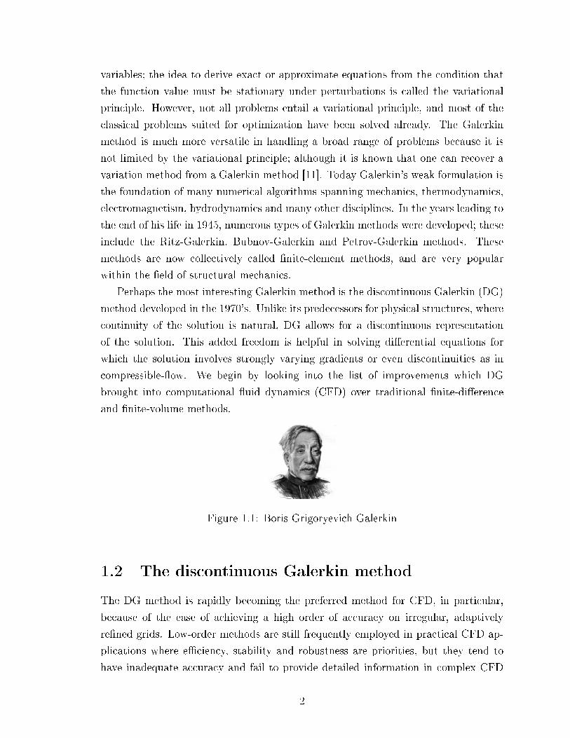
Figure 1.1: Boris Grigoryevich Galerkin
1.2 The discontinuous Galerkin method
The DG method is rapidly becoming the preferred method for CFD, in particular,
because of the ease of achieving a high order of accuracy on irregular, adaptively
rened grids. Low-order methods are still frequently employed in practical CFD ap-
plications where eciency, stability and robustness are priorities, but they tend to
have inadequate accuracy and fail to provide detailed information in complex CFD
2

problems. Therefore, the CFD community is now focusing on high-order methods
where very accurate results obtained at a reasonable cost yield computational e-
ciency. DG achieves high order by increasing the number of subcell data, hence the
increase in the order of accuracy is realized within a single cell instead of by interpola-
tion between cells, as in traditional nite-volume and nite-dierence methods. The
trouble with high-order nite-volume and nite-dierence methods is twofold. In the
rst place, constructing a highly accurate interpolant based on data on an unstruc-
tured, adaptively rened grid calls for great code complexity. In the second place, it
requires a dramatic increase in stencil size, which in turn causes complications near
the boundary of the computational domain and also at internal boundaries between
subdomains handled by dierent processors. The problem with high-order interpola-
tion near the domain boundary is often resolved with the introduction of many layers
of ad-hoc ghost elements, or with a highly skewed stencil which may imperil stability.
With regard to domain decomposition, long-range element interconnectivity heavily
burdens the data-link communication between computer nodes in a parallelized com-
puter architecture. As a result, the traditional high-order methods based on wide
interpolation stencils are no longer desirable on highly unstructured grids. The com-
pactness of DG is arguably better suited for today's computer architectures and for
complex CFD problems.
We start with outlining the mathematical principles of the DG method; the cor-
responding numerical discretization will be discussed later. The method of primary
interest for uid dynamics is the weighted-residual method. The general concept is to
project the entire problem from an innite solution space onto a nite solution space.
The terms solution space and projection are central to understanding Galerkin
methods. Ideally, one would work with an innitely large solution space to obtain
the complete information about the solution, but that would take innite computing
time. By working with a smaller solution space, we are accepting a certain degree
of error in our solution. The mathematical notion for transforming the solution from
one solution space to a smaller one is called projection (see Appendix A for more
information). The projection operator, a result of the inner product, integrates the
product of the solution and the basis functions of the smaller solution space.
In order to facilitate our discussion, the simple 1-D linear diusion equation is
provided as an example,
Ut − (DUx)x = 0, (1.1)
or
Ut = DUxx, (1.2)
3
where D is a constant. The weighted-residual formulation is obtained by multiplying
the PDE with a test function (or weighting function) v and integrating over the entire
physical domain D, ∫DvUt dx = D
∫DvUxx dx. (1.3)
This operation is also known as the inner product of v and Ut. The intent is to do this
with a whole space of test functions. We introduce the residual R, of the governing
equation as ∫DvR dx =
∫DvUt dx−D
∫DvUxx dx = 0. (1.4)
By enforcing the residual to be equal to zero, this weighted-residual formulation
provides the necessary equations to solve for the unknowns. Let us now step down
from the full solution U to an approximate solution u. First we focus on the denition
of the solution space of v and u. The solution space is described by the order of the
polynomial p, and a solution space capable of representing polynomials up to degree
p is mathematically denoted as Pp, where P is polynomial space. The solution space
is spanned by basis functions. One can view basis functions as building blocks of
a solution space, where any polynomial of order P can be constructed by a linear
combination of basis functions. If the test function v belongs to the same solution
space as u, then we have the Galerkin method.
The concept of test-function space and solution space may seem daunting at rst,
but the concept is elegantly simple and powerful. Let u be a function of x. If we
integrate the product of u with a zeroth-degree test function, v (x) = 1, over the
domain D, we will extract the average of u. Similarly, if we take the inner product
of u with a rst-degree test function, v (x) = x, we will extract the average rst
derivative. If we repeat this process for higher and higher-order test functions, we
will be able to extract higher-degree average derivatives from u. Repeating this
process innitely many times will allow us to know everything about u and the PDE.
However, with limited computational resources, we are forced to work in a nite
solution space. Thanks to Galerkin's weak formulation, we can solve the PDE within
the solution space and ignore the high-order information that lies in the complement
space. The complement space is strictly orthogonal to the solution space, and hence
conveniently it contains the error in the solution. The ocial weak statement reads:
Let u be a solution in W , and v be a test function in V , then u must satisfy the
partial dierential equation tested with v. Again, if W = V , we have the Galerkin
method. We are now ready to introduce the discontinuous Galerkin discretization.
4

Discretization in CFD means dividing up the physical domain D into smaller non-
overlapping elements Ωj, such that D =∑
j Ωj. Each Ωj contains a solution space
valid within the element boundary only, or simply called a solution with compact
support. In this example, let uj be the discretized solution of degree p within Ωj,
and uj = 0 outside of Ωj. In the continuous Galerkin (CG) method, the solution
must be continuous across an element interface, while in DG, the solution allows for
a discontinuity across the element interface. We emphasize the solution within each
element of DG is continuous, it only jumps across the interfaces. Figure 1.2 shows
two types of piecewise-linear solution representation in 1-D.
Ωj Ωj + 1Ωj - 1 Ωj Ωj + 1Ωj - 1
xj - 1/2 xj + 1/2xj - 1/2 xj + 1/2
Figure 1.2: Continuous Galerkin (left) and discontinuous Galerkin (right) solutionrepresentations showing the key dierence is the requirement of continuityacross element interface
The concepts of solution space and weak formulation are now applied to each
individual element,∫D
vut dx =∑j
∫Ωj
vjuj,t dx =∑j
D
∫Ωj
vjuj,xx dx. (1.5)
We obtain the global solution over D by locally solving for uj in every element. Notice
the test function, vj, can now be locally dened inside each cell,
vj =
v x ∈ Ωj
0 x /∈ Ωj
. (1.6)
We can also say vj has compact support. Note that this doesn't mean vj is undened
outside the cell; it is just strictly zero beyond the cell boundary. DG is a truly com-
pact method where each element interacts only with its immediate neighbors. This
interaction occurs through the ux, when conserved quantities ow across the element
interface. The ux between two elements provides the necessary element coupling,
and is central to tying the local solutions together to form one global solution. In the
PDE 1.1 the ux equals −DUx. Let us focus on the weak equation of one cell only,
and apply integration by parts once to introduce element coupling at the element
5

interface, ∫Ωj
vjuj,t dx = D [vjuj,x]xj+ 1
2xj− 1
2−D
∫Ωj
vj,xuj,x dx, (1.7)
where the notation [·]xj+ 1
2xj− 1
2represents a dierence across the element from xj+ 1
2to xj− 1
2
(see Figure 1.2). However, in the DG method neither the solution nor its derivatives
are well-dened at the element interface. If one takes the derivative value within the
element, there will be no element coupling. Hence we need to replace the non-unique
solution at the element interface with a unique solution, u(j,j+1) = u (uj, uj+1). The
ux value at the element interface is always a function of the two solutions sharing
that interface, hence the nal discretized equation reads,
∫Ωj
vuj,t dx = D(vj
(xj+ 1
2
)u(j,j+1),x − vj
(xj− 1
2
)u(j−1,j),x
)−D
∫Ωj
vj,xuj,x dx, (1.8)
where vj
(xj± 1
2
)is evaluated inside Ωj. Deriving a good numerical-ux algorithm is
not an easy task, and is the subject of extensive research. In fact, the rst major
subject of this thesis, RDG, is a very recent (2005) addition to the family of DG
diusion uxes. Furthermore, Eqn 1.8 is only a semi-discretization; it requires a
matching time-marching method. The second large subject of this thesis, HH-DG,
deals with this aspect of DG. We continue with a short history of DG for advection
and diusion, highlighting both spatial discretizations and marching in time.
1.3 History of advection and explicit time-marching
methods for DG
The DG approach was originally developed for the steady neutron-transport equations
by Reed and Hill (1973) [32]; their formulation was impressively general, being based
on a structured triangular grid and going up to p = 6. Immediately, LeSaint and
Raviart [22] proved that the order of accuracy of steady 1-D DG advection solutions
is 2p + 1; this order is found even for unsteady Euler solutions (see Section 6.2.2).
Later, Johnson and Pitkaranta [21] showed the order of accuracy on general triangular
elements is p + 12. Independently, Van Leer (1977) [37] introduced a time-accurate
DG method for scalar advection, replicating the exact shift operator. Since then, few
attempts were made to improve upon the time marching aspect of the DG machinery.
6

The procedure to extend the order of spatial discretization in a DG method is simple
and elegant, however, a matching temporal discretization for arbitrarily high order
proved to be far more dicult, as evident by the lack of progress in the following
decade.
Eventually, Cockburn and Shu (1989) [7] extended the spatial DG discretization
method to uid dynamic equations by coupling it with Runge-Kutta time-marching,
yielding the RK-DG scheme. Cockburn and Shu's paper sparked a renewed interest in
using DG for CFD. Around this time, analysis on DG stability and accuracy started
to blossom and DG quickly matured. It is not uncommon to see newer DG methods
achieve an order of accuracy beyond 2p+ 2, e.g. the RDG and cRDG methods.
While RK-DG dominated the stage regarding time-marching for 15 years, the lim-
itation of RK time marching to 5th-order of accuracy [16] was felt as the aerospace
industry expressed its desire for high-order codes. A new class of time-marching
schemes based on Taylor-expansions in time was developed; these include the ar-
bitrary order using derivatives DG method (ADER-DG) [10], space-time-expansion
DG (STE-DG) [15], the upwind moment scheme (UMS) [17] and the Hancock-Huynh
discontinuous Galerkin (HH-DG) method. Extension to high order for these methods
is automatic and requires less memory than traditional RK-DG methods; however,
an adverse eect on the CFL number for ADER-DG and STE-DG may render them
slower than RK-DG. Only UMS and HH-DG improve the CFL-number range over
RK-DG, which renders them potential candidates for replacing these popular meth-
ods. We describe the works of the authors mentioned above in chronological order.
1.3.1 The original DG: neutron transport
In 1973 Reed and Hill [32] demonstrated the rst successful use of a DG spatial
discretization for steady-state neutron transport problems on 2-D orthogonal trian-
gular meshes. In their landmark paper they argued the superiority of discontinuous
Galerkin over the commonly used continuous Galerkin (CG) method. The dierence
between the two methods lies in the continuity requirement across element interfaces.
The CG method enforces the C0 condition, meaning that the function value must be
continuous while the derivatives are allowed to jump across the interface.
Reed and Hill showed a p-th order DG method achieves the same error level (or
lower) than a (p + 1)-st order CG method. The p-th order DG method required
slightly more CPU time than its p-th order continuous counterpart on a 200-element
grid; however, the DG method appeared faster on the 800-element grid. The issue
7
of superiority of DG over CG was not clear until Reed and Hill tested problems
containing optically thick regions. Schemes based on continuous solutions were well
known to produce ux oscillations, however, DG quickly damped the oscillations
toward the nite medium solution and exhibited remarkable stability in comparison
to CG. The phenomenal spatial resolution of DG was clearly demonstrated by Reed
and Hill; however, it would be 16 years before DG was fully ready for time-accurate
problems.
1.3.2 Van Leer's schemes III & VI
Van Leer pioneered the concept of an exact shift operator in 1977 [37] for DG. He
replaced the initial-value solution per mesh with an approximate solution and con-
vected the resulting distribution exactly for the scalar advection equation (named
convection at that time). He constructed various schemes that allow for disconti-
nuity of the solution; in particular, his scheme III and VI are really piecewise-linear
and piecewise-quadratic DG schemes. Independent of Reed and Hill's development,
Van Leer recognized the need for separate update equations for the higher moments
at the cost of extra computational resources. The resulting advection method is fully
explicit and time-accurate. A Fourier-analysis showed the order of accuracy of scheme
III to be three. Van Leer did not analyze scheme VI due to its sheer complexity and
also thought it unattractive because of its high storage requirement, especially in
multi-dimensions, an issue that seems trivial for today's computer, but forbidding to
the computers of the 1970's. Although the paper's title mentions dierence schemes,
schemes III and VI were the rst time-accurate DG methods and could be easily
extended to arbitrarily high order. When trying to extend his schemes to a nonlinear
system of conservation laws, Van Leer ran into problems with the time integration
and he abandoned the project. Over the next one-and-a-half decade, various research
eorts focused on extending RK-DG's time accuracy to orders of ve and beyond,
and increasing the allowable CFL number. Interestingly, Van Leer's III & VI schemes
were reinvented in the atmospheric sciences and used for species transport [31, 34].
But it took 27 years before a correct extension of scheme III to the Euler equations
was presented (UMS).
1.3.3 Runge-Kutta methods
Runge-Kutta methods are an important family of explicit and implicit multi-stage
methods for approximating the solution of ordinary dierential equations. The method
8

was developed by German mathematicians C. Runge and M.W. Kutta around 1900
[47]. Jameson, Schmidt and Turkel [20] incorporated the 4-stage Runge-Kutta (RK)
method in their nite-volume code for the Euler equations in 1981. The method was a
huge improvement over existing multi-stage and other nite-dierence Euler methods
due to the sharpness of captured shocks, and the explicit convergence-acceleration
techniques included. RK is an extremely user-friendly time discretization; anybody
can pick up an ordinary-dierential-equations textbook and implement RK methods
without the need to know the details. The same spatial operator is applied at each
stage. Stages can be added or modied to increase order of accuracy in time, or to
enlarge the stability domain for achieving a higher CFL number.
The RK method was ported into the DG framework by Cockburn and Shu [7] for
advection in 1989. The RK temporal discretization and the DG spatial discretization
work very well together, since both discretization are compact and can be formally of
high order. Although it appears that an n-stage RK method only uses information
from immediate neighbors, the actual stencil is much larger since each immediate
neighbor also borrows information from neighboring elements. The end result is a
pyramid structure in space and time involving 2n+ 1 elements in 1-D. Nevertheless,
the coupling of RK and DG results in a stable and sharp shock-capturing method
called RK-DG. The authors prove RK-DG to be total-variation-bounded in the means
(TVBM), which implies the method allows new local extrema to occur within the
element, but not in the mean.
1.3.4 ADER and STE-DG methods
A group of German scientists focused exclusively on developing low-storage time-
marching schemes for DG. The storage requirement for RK-DG becomes severe as
the order of the solution polynomial increases, and as the number of stages of the RK
method increases. Besides the memory issue with RK-DG, the extension to very high
order [37] is extremely cumbersome. Followers of RK-DG must refer to lengthy tables
to implement each stage of an RK-DG method. Dumbser and Munz [10] ported the
ADER-FV (Arbitrary order using derivatives for nite volume) method into DG and
knighted the scheme as ADER-DG. The key component of ADER is to Taylor-expand
the solution in both space and time, and then convert the time and cross-derivatives
into spatial derivatives with the Cauchy-Kovalevskaya or Lax-Wendro procedure.
With the solution expressed in terms of both space and time variables, the governing
equation is then integrated in both space and time analytically. The Taylor expansion
9
in space and time to any order is fully automated, hence ADER-DG ts nicely into
the DG machinery.
In 2007, Lörcher, Gassner and Munz [24, 15] introduced space-time expansion DG
(STE-DG) as a modication of ADER-DG to account for grids with a large variation
in element size. The analytic integration in time is now replaced with Gaussian
quadrature to allow for exibility in time-stepping. The ux values are obtained
from the Taylor expansion of the solutions on both sides of the element interface,
and a Riemann solver is used at the designated temporal Gaussian points. Both
methods are suited for time-step adaptation, i.e, using multiple small time steps
in small cells to catch up with the marching in large cells. Logic gates must be
implemented to keep track of the order in which elements are updated. Despite the
slight overhead in logic, the reduction in CPU time on multi-scale grids is signicant.
Such adaptive time-stepping does not take away local conservation from the scheme,
while STE-DG is time-accurate to the order p+ 1. The memory requirement to store
all the ux values at the Gaussian points in time is signicantly less than for RK-DG.
Despite all the improvements over RK-DG, ADER-DG and STE-DG fail to address
the fundamental issue of stability, that is, the pursuit of the maximum time step.
In fact, both ADER-DG and STE-DG have a much tighter CFL limit than RK-DG,
rendering these space-time methods highly inecient on structured grids.
1.3.5 Huynh's upwind moment method
In the same year STE-DG was introduced, Huynh introduced the Upwind Moment
scheme (UMS) for conservation laws [17]. Huynh's scheme is based on Van Leer's
Scheme III [37] for advection, which applies the exact shift operator to the initial val-
ues. Huynh extended Van Leer's Scheme III to the Euler equations for piecewise-linear
solutions by making Hancock's predictor-corrector method, previously used only with
interpolated subcell gradients, suited for DG; the key lies in treating the space-time
volume integral accurately. The solution is marched to the half-time level by a subcell
Taylor-series expansion, after which the time-centered ux is calculated with upwind
data or, in general, a Riemann solver. UMS is extremely simple, 3rd-order accurate,
and realizes exact one-mesh-translation for linear advection at a CFL number of unity.
Suzuki [36] successfully adapted UMS to hyperbolic-relaxation systems in 2008.
10
1.3.6 Hancock discontinuous Galerkin method
In 2009, we extended Huynh's UMS method to arbitrary order and also incorporated
the recovery procedure (RDG) for diusion. The method is named Hancock-Huynh
discontinuous Galerkin (HH-DG); UMS is included in it. The design of HH-DG is
guided by Hancock's observation (1980): the solution can be advanced within a cell
with any complete set of ow equations; it is the interface ux that must describe the
interaction of adjacent cells. This rule is also observed in ADER-DG and STE-DG.
Huynh added to this that in DG the space-time volume integral must also be aected
by the cell interactions. This inuence is missing in ADER and STE-DG. HH-DG
has demonstrated remarkable reliability in dealing with the Euler equations and with
the scalar diusion equation; the order of accuracy is 2p + 1 for time-accurate Euler
in 1-D and 2p + 2 for time-accurate 1-D diusion. Like UMS, HH-DG reduces to
the exact shift operator for the scalar advection equation. Even in the nonlinear
advection case, HH-DG remains stable with a CFL number of unity. This is by far
the fastest explicit time-marching DG scheme in development; our current research
is focused on increasing the speed of HH-DG for diusion.
1.4 History of diusion methods for DG
DG combines the local discontinuous solution representation of a nite-volume scheme
with the compactness and versatility of a nite-element scheme. DG captures discon-
tinuous hyperbolic phenomena such as contact discontinuities, slip surfaces and shock
waves naturally with its discontinuous basis functions; however, discontinuous basis
functions are not the natural way to handle the diusion operator. Development in
DG methods for the diusion operator became successful starting with Arnold (1982)
[2], who introduced a penalty term to penalize discontinuities at the cell interfaces.
Much later Baumann (1998) [28] designed a stable DG method without that penalty
term, but the enthusiasm for this method died out soon. Bassi and Rebay (1997)[4]
and Cockburn and Shu (1998) [8] introduced the highly parallelizable BR2 and lo-
cal discontinuous Galerkin (LDG) methods, respectively, for the advection-diusion
equation, and were able to reach high orders of accuracy. Arnold [3] showed that all
diusion schemes for DG (as of 2002) could be expressed in terms of a sequence of
bilinear terms with scheme-specic coecients.
In 2005, Van Leer and Nomura [44] introduced a discontinuous Galerkin method
based on the recovery concept (RDG). RDG was completely dierent from any pre-
11
existing methods, conceptually simpler and extremely high-order. Gassner, Lörcher
and Munz [14] (2006) developed a diusion ux that derives from the exact solution
of the generalized diusive Riemann problem; this approach loses consistency when
reducing the time-step without rening spatially. Recently, Huynh [18, 19] developed
a family of diusion schemes which incorporate LDG, BR2 and RDG. His technique
of using dierent correction functions allows him to develop and experiment with new
diusion schemes. Owing to his detailed analysis and numerical experiments, we are
able to compare dierent diusion methods in a head-to-head manner. The following
sections detail in chronological order the major developments in diusion for DG.
1.4.1 The (σ, µ)-family
In the early days, DG had ridden on the success of adopting Riemann solvers for
the ux computation from nite-volume methods for hyperbolic equations. However,
when it came to parabolic and elliptic equations, the DG community was at a loss.
One of the rst attempts to solve parabolic and elliptic equations with DG is credited
to a venerable class of schemes called the (σ, µ)-family:
∫Ωj
vut dx = −D(< ux > [v] |j+ 1
2+ < ux > [v] |j− 1
2
)−D
∫Ωj
vxux dx
+ σD(< vx > [u] |j+ 1
2+ < vx > [u] |j− 1
2
)− µD
∆x
([v][u] |j+ 1
2−[v][u] |j− 1
2
). (1.9)
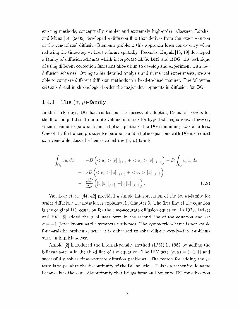
Van Leer et al. [44, 42] provided a simple interpretation of the (σ, µ)-family for
scalar diusion; the notation is explained in Chapter 3. The rst line of the equation
is the original DG equation for the time-accurate diusion equation. In 1979, Delves
and Hall [9] added the σ bilinear term in the second line of the equation and set
σ = −1 (later known as the symmetric scheme). The symmetric scheme is not stable
for parabolic problems, hence it is only used to solve elliptic steady-state problems
with an implicit solver.
Arnold [2] introduced the internal-penalty method (IPM) in 1982 by adding the
bilinear µ-term in the third line of the equation. The IPM sets (σ, µ) = (−1, 1) and
successfully solves time-accurate diusion problems. The reason for adding the µ-
term is to penalize the discontinuity of the DG solution. This is a rather ironic name
because it is the same discontinuity that brings fame and honor to DG for advection
12
problems. These bilinear terms are added to the diusion equation to increase the
chances of coming up with a stable method, while consistency with the governing
equation seems to be secondary. Van Leer and Nomura pointed out that for p = 0
the (σ, µ)-family is only consistent with the diusion equation owing to Arnold's
penalty term and only if µ = 1. In retrospect, Arnold did accurately determine the
need for an additional bilinear term. In 1997, Baumann and Oden [28] presented
the choice of (σ, µ) = (1, 0), representing a complete sign change from the symmetric
scheme and abandonment of Arnold's term. The freedom to switch to totally dierent
values of (σ, µ) over the course of two decades clearly indicates there existed no good
guiding principle for choosing the right set of coecients. In the early stages of our
research in RDG, we were able to nd an inkling of a relationship between RDG and
the (σ, µ)-family for p = 1; this is further extended in Section 3.3.5. The progress in
diusion for DG was painfully slow until the beginning of the 21st century. The next
set of methods marks the rst departure from the (σ, µ)-family.
1.4.2 Approaches based on a system of rst-order equations
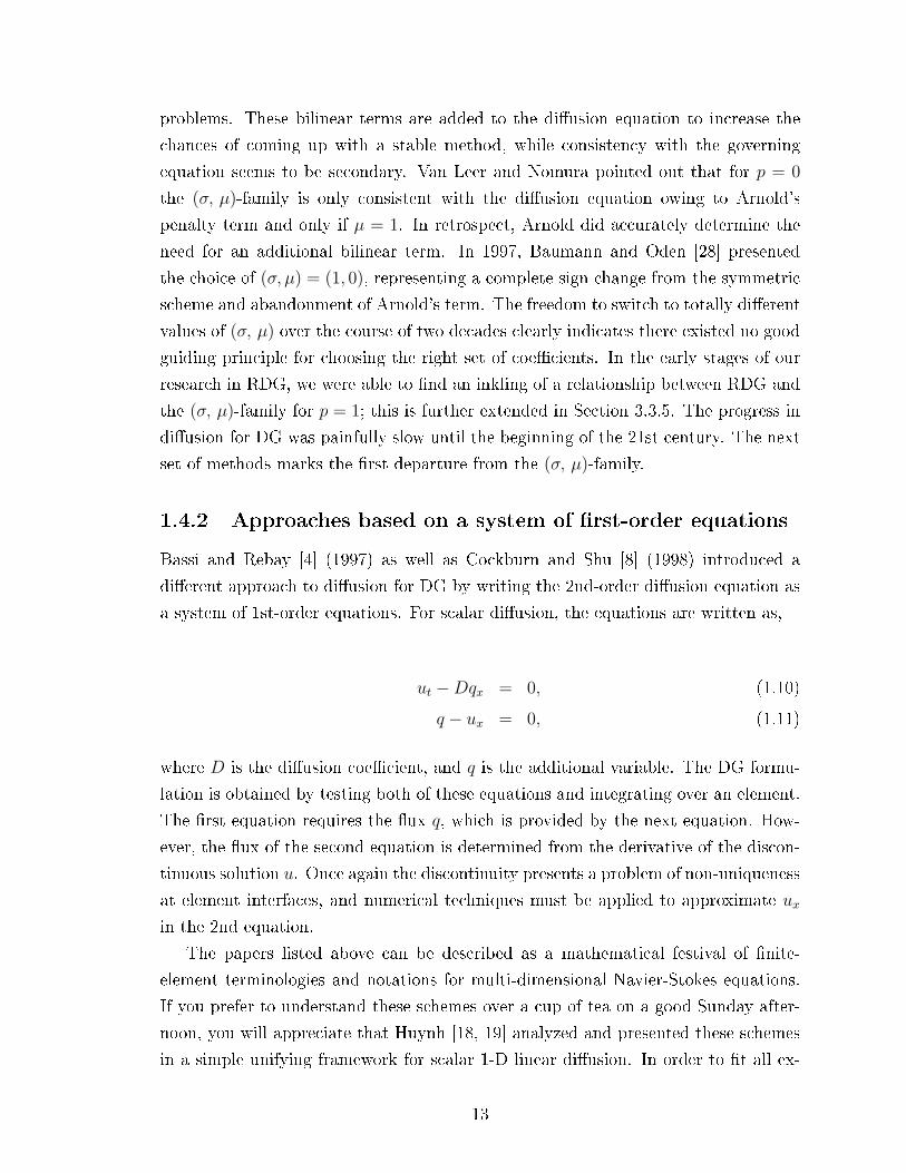
Bassi and Rebay [4] (1997) as well as Cockburn and Shu [8] (1998) introduced a
dierent approach to diusion for DG by writing the 2nd-order diusion equation as
a system of 1st-order equations. For scalar diusion, the equations are written as,
ut −Dqx = 0, (1.10)
q − ux = 0, (1.11)
where D is the diusion coecient, and q is the additional variable. The DG formu-
lation is obtained by testing both of these equations and integrating over an element.
The rst equation requires the ux q, which is provided by the next equation. How-
ever, the ux of the second equation is determined from the derivative of the discon-
tinuous solution u. Once again the discontinuity presents a problem of non-uniqueness
at element interfaces, and numerical techniques must be applied to approximate ux
in the 2nd equation.
The papers listed above can be described as a mathematical festival of nite-
element terminologies and notations for multi-dimensional Navier-Stokes equations.
If you prefer to understand these schemes over a cup of tea on a good Sunday after-
noon, you will appreciate that Huynh [18, 19] analyzed and presented these schemes
in a simple unifying framework for scalar 1-D linear diusion. In order to t all ex-
13

isting schemes into a unifying framework, Huynh used integration by parts twice on
the scalar diusion equation and applied dierent correction functions to calculate
the common function value and derivative value across the element interface. His
interpretation of the Bassi-Rebay schemes for diusion, also known as BR1 and BR2,
is shown in Figure 1.3.
Ωj Ωj + 1 Ωj Ωj + 1
gL
gR
gL
gR
Figure 1.3: Interpretation of BR1 (left) and BR2 (right) for scalar 1-D diusion. Twonew local solutions are reconstructed on the left and right of the indicatedinterface as gL and gR respectively. The large solid dot indicates theaverage of the left and right values at the interface. The schemes alsoadopt the average of the derivative values as the interface value of ux.Notice BR1 utilizes a 4-cell stencil for an interface ux, while the newerBR2 utilizes a 2-cell stencil.
Ωj Ωj + 1
gL
gR
Ωj Ωj + 1
gL
gR
Figure 1.4: Interpretation of two versions of LDG for scalar 1-D diusion. Two newlocal solutions are reconstructed on the left and right of the indicatedinterface as gL and gR respectively. The large solid dot indicates thecommon function value. The LDG is a non-symmetric scheme using thefunction value of gL for u, but the derivative value of gR for ux, (left) orvice versa (right).
For each interface, two functions gL and gR of order p + 1 are reconstructed by
sharing most moments with the original solution in their respective elements. In
BR1, the functions g in each element must satisfy Dirichlet conditions at both left
and right interfaces. The Dirichlet condition is simply to satisfy the average solution
value across the interface, which leads to a clumsy and costly 4-cell stencil. Bassi and
Rebay introduced the simpler BR2 version in which each g only needs to satisfy one
cell-coupling Dirichlet boundary condition and one local Dirichlet boundary condition.
The g functions in both BR1 and BR2 take the same function value at the interface,
14

but not the same derivative value. Bassi and Rebay then used the arithmetic mean
of ∂gL∂x
and ∂gR∂x
to approximate ux. Cockburn and Shu's Local DG (LDG) scheme for
scalar diusion is shown in Figure 1.4. The pair of g functions share most moments
with the solution in their respective elements. One of the intervals provides the
solution value at the interface; the g function in the other interval then provides the
desired solution derivative. Thus, there are two variants of the 1-D LDG scheme.
As Huynh indicated, Bassi-Rebay and Cockburn-Shu have dierent interpretations of
the common function value and function derivative value. Huynh studied several
other choices to be detailed later.
In 2008, Peraire and Persson [30] reduced the storage requirement and stencil size
of LDG and called their new scheme Compact DG (CDG). The paper compared BR2,
LDG and CDG and showed LDG and CDG have roughly the same spectral radius,
while BR2's spectral radius is about 1.5 times greater, meaning a narrower stability
range for the time step. Although CDG is exactly the same as LDG in 1-D, the
storage requirement is dramatically reduced for higher spatial dimensions.
1.4.3 Recovery-based discontinuous Galerkin method
RDG was introduced in 2005 by Van Leer and Nomura [44], and subsequently ex-
panded in [43, 41]. Central to RDG is the concept of recovery between two elements
where the solution is discontinuous. RDG recovers a smooth function in the union
of the two elements that is indistinguishable from the original solutions in the weak
sense. RDG demonstrated a remarkable order of accuracy for scalar diusion equa-
tion on structured grids. Our current research eort focuses on adapting RDG to
nonlinear diusion problems on unstructured grids. A full treatment to RDG begins
in Chapter 2.
1.4.4 Flux-based diusion approach
In 2006, Gassner, Lörcher and Munz [14] introduced a numerical diusion ux based
on the exact solution of the diusion equation at the discontinuity of a piecewise con-
tinuous solution. The concept is similar to that of Godunov-type nite-volume meth-
ods for hyperbolic equations. The diusive generalized Riemann problem (dGRP) can
be solved for any order of the solution space. The ux is obtained from the general
bounded solution of the discontinuous initial-value problem for the diusion equa-
tion and depends on both space and time. The resulting dGRP-DG is a space-time
method for diusion. However, the dGRP ux is only consistent if ∆x ∝ ∆t. The
15

scheme uses the time integral of the diusion ux for the update; the time average of
the ux always contains a term proportional to 1/√
∆t. For ∆t → 0, while keeping
∆x xed, the ux blows up, rendering the scheme sensitive to small time steps; the
ux is unsuited for combination with multi-stage time integration. The dGRP-DG
scheme performs relatively fast in steady-steady problems, as the stability limit on
∆t is proportional to ∆x only instead of the usual (∆x)2 for explicit methods. In
addition, Gassner et al. were able to express the dGRP-DG scheme in bilinear terms,
and discovered dGRP-DG shared many terms with the (σ, µ)-family. The scheme
has a µ coecient dierent from the one in the symmetric interior-penalty method,
and contains an additional bilinear term of the form
< vx > [ux] |j+ 12− < vx > [ux] |j− 1
2. (1.12)
Gassner et al. observed that the presence of the new higher-order bilinear term
increases the stability limit, however, the increase in stability limit decreases for higher
p. This is an important observation pertinent to the recovery-based discontinuous
Galerkin (RDG) method, as we shall show in a later chapter that the RDG method
automatically generates these higher-order bilinear terms.
1.4.5 Huynh's reconstruction approach
Huynh studied a family of diusion schemes using his reconstruction approach [18, 19].
The concept is to reconstruct correction functions to correct for the discontinuity of
the solution across element interface. One of Huynh's primary motivations is to come
up with a scheme that replicates the success in accuracy and stability of RDG, while
reducing the computational cost. To this end, Huynh limited his correction functions
to one element only, and coupled the correction functions at the interface, whereas
in RDG, the single recovery function spans two elements and naturally couples the
elements. Huynh studied 16 dierent ways to couple the correction functions sharing
the same interface. One of the most promising new methods is, I-continuous - gLe/
SP - gDG, or aptly called Poor-man's recovery. Instead of dening a common func-
tion value and common derivative, the Poor-man's method naturally obtains these
values by solving a small system that couples the left and right correction functions.
The method is computationally cheap and achieves a higher order of accuracy than
existing BR2 and LDG methods. While comparison with RDG still demonstrates
RDG's superiority in accuracy and stability, it is worthwhile to further study how
these schemes compare to each other in terms of CPU time in a real time-accurate
16
calculation.
1.4.6 Combining DG advection with DG diusion
If one has satisfactory DG methods for discretizing the diusion and advection oper-
ators, it is a rather trivial task to combine the two in a DG method for advection-
diusion. Because of the fundamental dierences between these two operators and
their discretizations, such a blended advection-diusion method does not look at-
tractive. The advection and diusion discretizations are not consistent in their in-
terpretation of the numerical solution. For example, combining the upwind-biased
discretization, which fully accepts the discontinuous nature of the solution, with a
(σ, µ)-type discretization of the diusion term, which penalizes the solution for being
discontinuous, seems to reveal an inner conict.
A more ambitious approach would attempt to unify the solution representations
used for the dierent operators. Traditionally, a pure diusion operator is preferably
discretized with a continuous DG method, especially a nodal-point-based one where
it is trivial to guarantee that the solution representation is continuously dierentiable.
However, if one insists on a C(1) representation of the solution for the sake of diusion,
while linked to a primary discontinuous basis for advection, the relation between the
two ceases to be local. It leads to a global system of equations where the smooth
solution representation is based on the interface value and derivative of the solution;
the equation system will globally link these to the coecients of the interior basis
functions.
A recent example of a method that blends a C(1) interface-based solution to the
discontinuous cell-based solution is the HDG method of Cockburn et al. [6, 27].
Here the H stands for hybridizable, which appears to refer to the capability of the
method to be used along-side a continuous Galerkin method, used perhaps for other
equations of a system. This method combines the usual upwind DG discretization
for advection with a discretization of the diusion equation written as a system of
rst-order equations, similar to LDG (see Section 1.4.2). As explained before, this
method requires the solution of a global system; the authors point out, though, that
the unknowns are just the interface values, regardless of the order of the method.
In recovery-based DG, we also attempt the unication of the two solution rep-
resentations; however, it is a local unication. The smooth solutions recovered at
the interfaces of one cell overlap each other in the interior of the cell, but are not
equal; therefore, no global smooth recovered function exists. Given the high order of
17

accuracy achieved by RDG methods, it is doubtful that recovering a globally smooth
unique solution will bring any advantage. Moreover, it has been shown earlier by Van
Raalte and Van Leer [45] that the solution representation of the locally recovered
solution in the union of two cells is identical to the discontinuous solution once we
switch from the discontinuous basis to the smooth recovery basis; see also our paper
[41] on Unication of discontinuous Galerkin methods for advection and diusion.
1.5 Motivation
Our motivation directs us towards the ultimate discontinuous Galerkin scheme for
conservation laws. As of the year 2010, high-order compact methods such as DG
are poised to take over the nite-volume method which still counts as the industrial
standard. However, several issues still prevent the industry from moving away from
its safe in-house codes; DG is relatively new and has yet to establish a good record
of reliability. DG was dogged by its high storage requirement, the lack of a good
viscous discretization, lack of error estimation, lack of an ecient high-order time-
marching scheme, and lack of a multi-dimensional high-order-compatible limiter. We
are pleased to say that these issues are nearing resolution with a high level of con-
dence. This thesis focuses on resolving the issues of the viscous solver and ecient
time-marching for DG.
The design and presentation of current diusion schemes for DG is overly com-
plex and lacks physical interpretation. Numerical schemes were designed from the
standpoint of facilitating mathematical proofs instead of observing physical clarity.
Frustration is what drove us to design a new method that is a quantum level better
than existing methods. Van Leer and Nomura rst introduced the recovery-based DG
(RDG) method for diusion. The recovery concept is elegantly simple and, to their
surprise, achieved an order of accuracy beyond traditional superconvergence within
a generous stability range. Our rst goal is to further pursue the concept of recovery
and demonstrate RDG's ability to perform in multi-dimensional nonlinear diusion
problems.
In the eld of time-marching schemes for DG, nothing dramatic has risen above the
horizon since RK-DG. In fact, DG's high storage requirement drove researchers toward
implicit time-marching methods. Implicit time-marching methods naturally damp
eigenmodes and may not be time-accurate for all transient phenomena of interest.
Our goal is to design a fast, explicit, and high-order time marching scheme for DG. To
this end, we present the arbitrarily-high-order Hancock-Huynh discontinuous Galerkin
18

(HH-DG) method. HH-DG is a true space-time DG method in which spatial elements
are strongly coupled to temporal elements via a Cauchy-Kovalevskaya procedure. HH-
DG's true beauty comes from being the exact shift operator for linear advection, which
is a good starting point for a new scheme; it allows CFL numbers up to unity.
The rst half of the thesis is dedicated to introducing the recovery-based dis-
continuous Galerkin (RDG) method for diusion. In Chapter 2, we introduce the
recovery concept, and the weak formulation of the diusion equation with recovery,
then present a stability proof. The next two chapters detail RDG for 1-D and 2-D,
respectively, along with Fourier analyses and comparisons to other existing DG dif-
fusion schemes. Chapter 5 applies RDG to the Navier-Stokes equations and provides
numerical results to popular test cases. We introduce the new space-time DG method
called Hancock-Huynh discontinuous Galerkin (HH-DG) in Chapter 6, formulated to
accommodate both advection and diusion. In Chapter 7, we summarize our ndings
and point to a perspective of developments to be expected in the future.
1.6 Outline of this thesis: the River of Recovery
As an outline of this thesis, we oer Figure 1.5, the River of Recovery. It depicts the
main stream of our research as a river owing from the upper left to the lower right,
while broadening and with two cascades representing major obstacles in the progress
of the research. The river starts from the humble RDG-2x method for the 1-D linear
diusion equation and ends at the successful extension to the viscous terms of the
2-D Navier-Stokes equations. Along the way we present much Fourier analysis and
many failed schemes including those of the RDG-1x type. Numbers in parentheses
refer to thesis chapters.
Three side-streams are visible. One represents purely theoretical developments,
which do impact the main research as indicated by the merging of the side-stream
with the mainstream. Another stream represents the inuence of our work on others,
in particular the group at Idaho National Laboratory, which developed cell-centered
RDG (cRDG). This work eventually fed back into our own research by helping us
cross the nonlinearity cascades, as well as the cascades of cross-derivatives. Finally
there is the space-time DG stream which has led to arbitrary-order space-time DG
methods for advection and diusion separately, but not yet for advection-diusion in
a satisfactory way.
19

Theoretic
al S
tream
rd
g-2
x (
2,3
,4)
(Lin
ea
r D
iffu
sio
n)
hh
-dg
(6
)(S
pa
ce
-Tim
e A
dv
ec
tio
n)
hh
-rd
g (
6)
(Sp
ac
e-T
ime
Dif
fusio
n)
rd
g-1
x+
(3
,4)
(1-D
No
nli
ne
ar
Dif
fusio
n)
rd
g-1
x+
+ (
4,5
)(2
-D N
on
lin
ea
r D
iffu
sio
n w
ith
Cro
ss D
eri
va
tiv
es:
Na
vie
r-S
tok
es)
cr
dg
(2
,3,4
)(F
ull
So
luti
on
En
ha
nc
em
en
t)
st
ab
ilit
y p
ro
of
s (
2)
sig
ma
-mu
fa
mil
y (
3)
(p
en
al
ty
te
rm
s)
fo
ur
ier
an
al
ys
is (
3,4
)
bo
un
da
ry
tr
ea
tm
en
t (
3,4
)
rd
g-1
x f
am
ily
(2
,3,4
)
no
nu
nif
or
m g
rid
(4
)
No
nli
ne
ar
Ca
sca
de
s (3
,4)
Cro
ss-d
eri
va
tiv
es
(4)
Ca
sca
de
s
int
ro
(1
)
Figure
1.5:
Theoutlineof
thisthesisisrepresentedbytheRiver
ofRecovery.
20
CHAPTER II
Interface-centered Recovery-based
Method for Diusion
Recovery-based discontinuous Galerkin (RDG) is due to Van Leer and appeared on
the DG stage in 2005, marking the beginning of a new perspective on the diusion
operator for DG. The name recovery is attributed to K.W. Morton [26], who used it
in the context of shock recovery, which is the inverse process: recovering a discon-
tinuity from a smoothed prole. The further development of RDG was documented
in a train of papers [43, 41, 23, 45]. Unlike previous methods based on facilitating
mathematical proofs or choosing the correct values for the stability parameters, RDG
is based on a physical-numerical interpretation of the solution. The end product is a
universal concept of recovery that transcends its original purpose and can be applied
to dierent areas of DG and nite-volume methods. For this reason we sometimes
attach the term interface-based in front of RDG, iRDG, to indicate we are talking
about recovery for diusion; for most of this thesis, we will simply use RDG and
drop the i. This chapter rst describes the motivation behind RDG starting with
an interesting quote. We then cover various aspects of recovery concept and present
RDG for diusion. Next, we present stability proofs for various RDG methods for
scalar nonlinear diusion. The chapter ends with a brief talk on other uses of the
recovery concept.
2.1 The beginning of RDG
RDG literally began with Van Leer's observation, What's sauce to the goose is not
sauce to the gander. The original English idiom actually implies both genders should
be held to the same standards, but the word not was added to emphasize the funda-
21
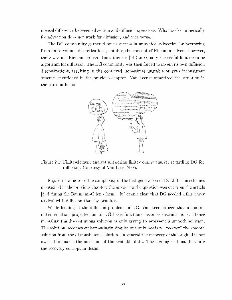
mental dierence between advection and diusion operators. What works numerically
for advection does not work for diusion, and vice versa.
The DG community garnered much success in numerical advection by borrowing
from nite-volume discretizations, notably, the concept of Riemann solvers; however,
there was no Riemann solver (now there is [14]) or equally successful nite-volume
algorithm for diusion. The DG community was then forced to invent its own diusion
discretizations, resulting in the contrived, sometimes unstable or even inconsistent
schemes mentioned in the previous chapter. Van Leer summarized the situation in
the cartoon below.
Figure 2.1: Finite-element analyst answering nite-volume analyst regarding DG fordiusion. Courtesy of Van Leer, 2005.
Figure 2.1 alludes to the complexity of the rst generation of DG diusion schemes
mentioned in the previous chapter; the answer to the question was cut from the article
[5] dening the Baumann-Oden scheme. It became clear that DG needed a fairer way
to deal with diusion than by penalties.
While looking at the diusion problem for DG, Van Leer noticed that a smooth
initial solution projected on to DG basis functions becomes discontinuous. Hence
in reality the discontinuous solution is only trying to represent a smooth solution.
The solution becomes embarrassingly simple: one only needs to recover the smooth
solution from the discontinuous solution. In general the recovery of the original is not
exact, but makes the most out of the available data. The coming sections illustrate
the recovery concept in detail.
22
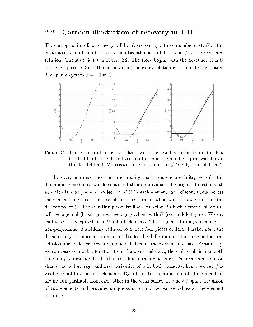
2.2 Cartoon illustration of recovery in 1-D
The concept of interface recovery will be played out by a three-member cast: U as the
continuous smooth solution, u as the discontinuous solution, and f as the recovered
solution. The stage is set in Figure 2.2. The story begins with the exact solution U
in the left picture. Smooth and untamed, the exact solution is represented by dotted
line spanning from x = −1 to 1.
−1 −0.5 0 0.5 10
1
2
3
4
5
6
7
8
9
10
x
U(x)
−1 −0.5 0 0.5 10
0.5
1
1.5
2
2.5
3
3.5
4
4.5
5
x
u(x)
−1 −0.5 0 0.5 1
0
0.5
1
1.5
2
2.5
3
3.5
4
4.5
5
x
f(x)
Figure 2.2: The essence of recovery. Start with the exact solution U on the left(dashed line). The discretized solution u in the middle is piecewise linear(thick solid line). We recover a smooth function f (right, thin solid line).
However, one must face the cruel reality that resources are nite; we split the
domain at x = 0 into two elements and then approximate the original function with
u, which is a polynomial projection of U in each element, and discontinuous across
the element interface. The loss of innocence occurs when we strip away most of the
derivatives of U . The resulting piecewise-linear functions in both elements share the
cell average and (least-squares) average gradient with U (see middle gure). We say
that u is weakly equivalent to U in both elements. The original solution, which may be
non-polynomial, is suddenly reduced to a mere four pieces of data. Furthermore, the
discontinuity becomes a source of trouble for the diusion operator since neither the
solution nor its derivatives are uniquely dened at the element interface. Fortunately,
we can recover a cubic function from the preserved data; the end result is a smooth
function f represented by the thin solid line in the right gure. The recovered solution
shares the cell average and rst derivative of u in both elements; hence we say f is
weakly equal to u in both elements. By a transitive relationship, all three members
are indistinguishable from each other in the weak sense. The new f spans the union
of two elements and provides unique solution and derivative values at the element
interface.
23
This story has a happy ending. The recovery concept presents a fresh way to
look at discontinuous solution in the union of two elements; and the example above
makes clear why this method is called recovery. Anyone understanding the recovery
principle may now stop reading and develop RDG entirely by himself or herself.
Regardless, we shall lay up next the mathematical foundation of recovery.
2.3 Interface recovery equations
We consider the most general framework inside an n-dimensional euclidean space, Rn.
Let D, the physical domain of interest, be a subspace in Rn. We introduce two vector
spaces: the solution space W and the test space V in D. Let φ be a set of smooth
functions with compact support satisfying W = φ ∈ W : φ ∈ P k (D) where Pp (D)
is the polynomial space of D containing polynomials of at most degree p. Similarly
let V = v ∈ V : v ∈ P k (D). The domain is discretized into non-overlapping
cells such that D =∑
j Ωj. If the solution space of V is the same as W , then this
is a Galerkin method; furthermore, if the basis functions are discontinuous across
the element interface, then this is specically the DG method. Let Ωj and Ωj+1 be
two elements sharing the element interface Sj,j+1, and their solutions be expressed
respectively as,
uj =
Nj∑i=1
aj,i φi, (2.1)
uj+1 =
Nj+1∑i=1
aj+1,i φi, (2.2)
where aj,i and aj+1,i are the degrees of freedom and the integers Nj and Nj+1 are the
number of degrees of freedom in Ωj and Ωj+1, respectively. We introduce the recovery
function, fj,j+1 centered on Sj,j+1 as,
fj,j+1 =
Nj+Nj+1∑i=1
bi ψi, (2.3)
where bi are the unknown coecients and ψi are the recovery basis functions spanning
the union of elements Ωj and Ωj+1. The proper choice of ψi is essential for a well-
conditioned recovery as will become clear soon. The recovery equations are of the
24
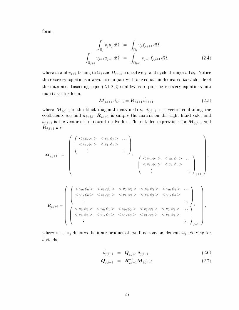
form, ∫Ωj
vjuj dΩ =
∫Ωj
vjfj,j+1 dΩ,∫Ωj+1
vj+1uj+1 dΩ =
∫Ωj+1
vj+1fj,j+1 dΩ. (2.4)
where vj and vj+1 belong to Ωj and Ωj+1, respectively, and cycle through all φi. Notice
the recovery equations always form a pair with one equation dedicated to each side of
the interface. Inserting Eqns (2.1-2.3) enables us to put the recovery equations into
matrix-vector form,
M j,j+1~aj,j+1 = Rj,j+1~bj,j+1, (2.5)
where M j,j+1 is the block diagonal mass matrix, ~aj,j+1 is a vector containing thecoecients aj,i and aj+1,i, Rj,j+1 is simply the matrix on the right hand side, and~bj,j+1 is the vector of unknown to solve for. The detailed expressions for M j,j+1 andRj,j+1 are
M j,j+1 =
< v0, φ0 > < v0, φ1 > . . .
< v1, φ0 > < v1, φ1 >...
. . .
j
< v0, φ0 > < v0, φ1 > . . .
< v1, φ0 > < v1, φ1 >...
. . .
j+1
,
Rj,j+1 =
< v0, ψ0 > < v0, ψ1 > < v0, ψ2 > < v0, ψ3 > < v0, ψ4 > . . .
< v1, ψ0 > < v1, ψ1 > < v1, ψ2 > < v1, ψ3 > < v1, ψ4 >...
. . .
j
< v0, ψ0 > < v0, ψ1 > < v0, ψ2 > < v0, ψ3 > < v0, ψ4 > . . .
< v1, ψ0 > < v1, ψ1 > < v1, ψ2 > < v1, ψ3 > < v1, ψ4 >...
. . .
j+1
,
where < ·, · >j denotes the inner product of two functions on element Ωj. Solving for~b yields,
~bj,j+1 = Qj,j+1~aj,j+1, (2.6)
Qj,j+1 = R−1j,j+1M j,j+1; (2.7)
25

Qj,j+1 is called the recovery matrix. The following sections detail how to choose ψi
to ensure that Rj,j+1 is fully ranked, and ways to reduce the condition number of
Rj,j+1.
2.3.1 Full-rank Rj,j+1
Choosing the correct recovery basis functions requires extra attention; perhaps it is
useful to think of this as a Tetris game. Tetris is a game where uniquely shaped blocks
fall downward due to gravity, and the blocks stack upon each other depending on
where the player chooses to drop them. Our recovery game follows the same rule.
The recovery function is composed of basis functions in the face-normal direction,
and in the face-parallel directions. The maximum order of basis functions in each
direction is dictated by the number of available data in each direction. Consider the
1-D examples for p = 0 and p = 1 in the gure below.
r2 r3rxx
r
1
11 1
1 1
Figure 2.3: A little block game for determining the recovery basis in 1-D. The blockson the left and right of the dashed line indicate basis functions of thesolution in Ωj and Ωj+1 respectively. Now imagine gravity pulls to theleft; the blocks from Ωj+1 fall on top of the blocks in Ωj to form therecovery basis.
The recovery basis functions are in the face-normal direction, or r-coordinate, and
the dashed line indicates the orientation of the element interface. For p = 0, only the
cell averages are available on each side of the interface; they are represented by the
1 blocks. If gravity pulls leftward, the two single blocks will stack up on each other
to form a two-block as shown in the gure to the right. The new two-block represents
two available data in the face-normal direction, hence recovery between two p = 0
elements results in a linear recovery function, indicated by the basis functions 1 , r.
Similarly, for p = 1, the two blocks with 1 and x represent the cell average and
gradient within each element. The recovery between two p = 1 elements results in a
four-block, or a cubic recovery function. In 2-D, the same strategy is followed, only we
now introduce the s-coordinate to account for solution variations in the face-parallel
26

direction. Consider the 2-D examples below for p = 1 and p = 2.
r2 r3r
xx r
1
11 1
1 x2xxyy
y2
1 x2xxyy
y2
yyr2 r3
ss2
sr sr2 sr3r4 r5
s2r
s sr
Figure 2.4: A little block game for determining the recovery basis in 2-D. The blockson the left and right of the dashed line indicate basis function of thesolution in Ωj and Ωj+1 respectively. Now imagine gravity pulls to theleft; the blocks from Ωj+1 fall on top of the blocks in Ωj to form therecovery basis. Notice there are more blocks in the r-coordinate than inthe s-coordinate.
Notice the recovery function includes twice as many basis functions in the r-
coordinate than in the s-coordinate in 2-D. This raises the question whether the
lower-order s-components of the recovery function will contaminate the high-order r-
components. The 2-D numerical results in Chapter 4 will provide a nuanced answer;
the details for triangular structured and unstructured grids will be spelled out later.
The concept of this block game may be childish, but plays an important role in
determining the rank of Rj,j+1. In the 2-D example for p = 1, if we naively attempt
to recover a complete quadratic recovery function from the six blocks in Figure 2.4,
Rj,j+1 will be rank-insucient, and the recovery process fails. The choice of recovery
basis is not ad-hoc, but follows an information conservation principle, where each
block in this game represents a piece of information the solution has in a certain
direction. If one can play with blocks, then one can perform recovery; the 3-D game
goes exactly in the same way. Achieving a full-rank matrix is the rst step; the next
step is to reduce the condition number of Rj,j+1.
2.3.2 Reducing the condition number of Rj,j+1
The reduction of the condition number of Rj,j+1 is central to reducing the magni-
tude of error and danger of instability of RDG. The conditioning number is the ratio
between the largest and smallest eigenvalues of the system; consequently, the lowest
achievable condition number is unity. There are two major ways to reduce the con-
dition number. The rst is the universal method of using a preconditioner to solve a
27
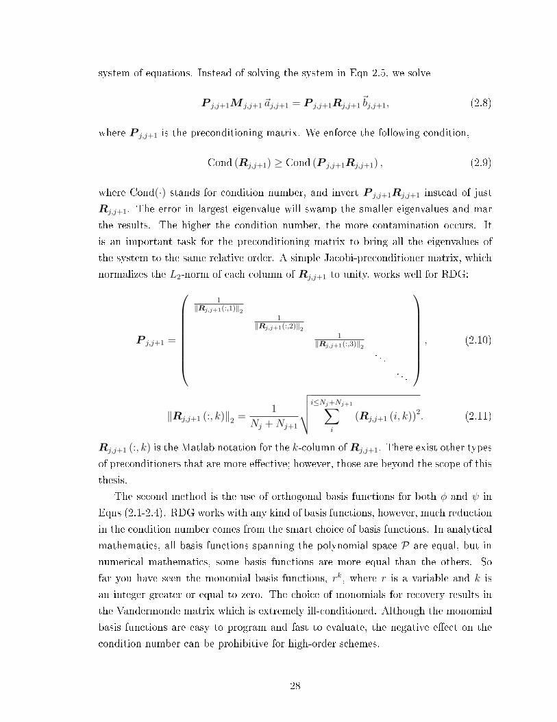
system of equations. Instead of solving the system in Eqn 2.5, we solve
P j,j+1M j,j+1~aj,j+1 = P j,j+1Rj,j+1~bj,j+1, (2.8)
where P j,j+1 is the preconditioning matrix. We enforce the following condition,
Cond (Rj,j+1) ≥ Cond (P j,j+1Rj,j+1) , (2.9)
where Cond(·) stands for condition number, and invert P j,j+1Rj,j+1 instead of just
Rj,j+1. The error in largest eigenvalue will swamp the smaller eigenvalues and mar
the results. The higher the condition number, the more contamination occurs. It
is an important task for the preconditioning matrix to bring all the eigenvalues of
the system to the same relative order. A simple Jacobi-preconditioner matrix, which
normalizes the L2-norm of each column of Rj,j+1 to unity, works well for RDG:
P j,j+1 =
1‖Rj,j+1(:,1)‖2
1‖Rj,j+1(:,2)‖2
1‖Rj,j+1(:,3)‖2
. . .. . .
, (2.10)
‖Rj,j+1 (:, k)‖2 =1
Nj +Nj+1
√√√√i≤Nj+Nj+1∑i
(Rj,j+1 (i, k))2. (2.11)
Rj,j+1 (:, k) is the Matlab notation for the k-column of Rj,j+1. There exist other types
of preconditioners that are more eective; however, those are beyond the scope of this
thesis.
The second method is the use of orthogonal basis functions for both φ and ψ in
Eqns (2.1-2.4). RDG works with any kind of basis functions, however, much reduction
in the condition number comes from the smart choice of basis functions. In analytical
mathematics, all basis functions spanning the polynomial space P are equal, but in
numerical mathematics, some basis functions are more equal than the others. So
far you have seen the monomial basis functions, rk, where r is a variable and k is
an integer greater or equal to zero. The choice of monomials for recovery results in
the Vandermonde matrix which is extremely ill-conditioned. Although the monomial
basis functions are easy to program and fast to evaluate, the negative eect on the
condition number can be prohibitive for high-order schemes.
28

Orthogonal basis functions are a very special class of basis with unique numerical
properties. The basis functions of an orthogonal set are completely independent
of each other; therefore, the mass matrix in Eqn 2.5 can be diagonalized for fast
evaluation. Furthermore, the elements of a diagonalized matrix are the eigenvalues;
hence a correct normalization of the orthogonal basis functions easily reduces the
condition number to unity. In 2-D we use a special orthogonal basis functions called
the Legendre polynomials for quadrilateral grids (see Section 4.1.3), and our own
orthogonal basis functions for triangular grids (see Section 4.1.3). In short, if φ is a
set of orthogonal basis functions on domain D, then∫Dφiφk dD = 0, i 6= k, (2.12)∫
Dφiφk dD 6= 0, i = k. (2.13)
Notice if we change the domain D, the relationship above no longer holds and or-
thogonality is lost. In our example below, the quadrilateral Legendre polynomials
(abbreviated as Q. Legendre) are orthogonal on the unit square domain; however, the
quadrilateral Legendre polynomials are not orthogonal on a unit triangle domain. For
recovery between two quadrilateral elements, using orthogonal Legendre basis func-
tions for the solution and monomials for the recovery basis functions generally results
in acceptable condition numbers. The best condition number achieved for quadrilat-
eral recovery is when both the solution and recovery basis functions are orthogonal
quadrilateral Legendre polynomials.
An elementary numerical study of recovery between triangular elements was per-
formed with various choices of solution basis functions, and with or without Jacobi-
preconditioner. We use the quadrilateral Legendre polynomials to illustrate the eect
of a poor basis for recovery between triangles, and compared that to a real orthogonal
basis for triangles. The results are detailed in the Table 2.1.
It is seen that the largest reduction in condition number is due to the correct
choice of solution basis functions and the preconditioner. We have eectively reduced
the conditon number by an order of magnitude when comparing the worst case to the
best case. Note that simple orthogonal recovery basis functions rarely exist in the
union of two elements except on Cartesian grids. Now that we have all the tools to
acquire and condition Rj,j+1, let us nd out the physical meaning embedded within
Rj,j+1.
29

Max Condition # φ ψ Jacobi Preconditioner
25 Orthogonal Triangular Monomial On40 Q. Legendre Monomial On116 Q. Legendre Monomial O286 Orthogonal Triangular Monomial O910 Q. Legendre Q. Legendre O
Table 2.1: Condition number of Rj,j+1 for recovery between two right triangular el-ements with p = 1 solutions. Notice quadrilateral Legendre polynomials(Q. Legendre) are no longer orthogonal on a triangle domain. Each faceof the triangle has a dierent condition number; the maximum conditionnumber of the three is reported.
2.4 Smooth recovery polynomial basis
Van Raalte and Van Leer [45] discovered the concept of a local smooth recovery
polynomial basis, which we call smooth recovery basis (SRB) for short. The term
local refers to the union of two elements and the term smooth dierentiates SRB
from the discontinuous solution basis. There exist an innite number of bases as
potential candidates for ψ in Eqn 2.3; however, there is only one unique basis such
that ~b = ~a in Eqn 2.5. We called this unique basis the SRB, ψ.
The existence of SRB allows us to interpret the discontinuous solution as a con-
tinuous solution. The two solutions are equivalent in the weak sense, but provide a
completely dierent picture at the element interface. SRB is always dened in the
union of the two elements; the discontinuous solutions are expressed in Eqn 2.1, and
the smooth solution is expressed as,
uj,j+1 =
Nj+Nj+1∑i=1
(~ai)j,j+1 ψi. (2.14)
The smooth solution inherits the coecients from the two neighboring discontinuous
solutions; we call this the Principal Recovery Theorem. Depending on the nature of
the problem, we may choose to use the discontinuous solution or the smooth solution.
SRB provides a unied treatment of the advection and diusion operator. The quest
to nd the members of SRB is not dicult; in fact they are hidden in Qj,j+1.
There exists one unique SRB for each choice of φ in Eqn 2.1. Let ψ in Eqn 2.3 be
anything as long as it satises the Tetris game mentioned in the previous section and
solve for Qj,j+1 in Eqn 2.6. The column vectors of Qj,j+1 span the vector space of ~b
and may therefore serve as a basis, or the SRB. The SRB is now expressed in terms
30

of the elements of Qj,j+1 as,
ψi =
Nj+Nj+1∑k
(Qk,i
)j,j+1
ψk. (2.15)
We consider two 1-D examples, for p = 0 (Figure 2.5) and p = 1 (Figure 2.6),
using the Legendre polynomials for φ. The domain of interest runs from 0 to 2, with
Ωj spanning from 0 to 1, and Ωj+1 spanning from 1 to 2.
0.0 0.5 1.0 1.5 2.0-0.5
0.0
0.5
1.0
1.5
x
fHxL
0.0 0.5 1.0 1.5 2.0-0.5
0.0
0.5
1.0
1.5
x
fHxL
Figure 2.5: In the p = 0 case, there is a total of two SRB functions. The smoothrecovery basis functions (solid lines) replacing vj = 1 (dashed lines) in Ωj
(left), and vj+1 = 1 in Ωj+1 (right).
0.0 0.5 1.0 1.5 2.0
-1.5
-1.0
-0.5
0.0
0.5
1.0
x
fHxL
0.0 0.5 1.0 1.5 2.0
-0.5
0.0
0.5
1.0
1.5
x
fHxL
Figure 2.6: In the p = 1 case, there is a total of four SRB functions. The smoothrecovery basis functions (solid lines) replacing vj = 1 and vj = 2ξ − 1(dashed lines) in Ωj (left), and vj+1 = 1 and vj+1 = 2ξ−1 in Ωj+1 (right).
It is seen the SRB functions, though indistinguishable in a weak sense from the
discontinuous basis functions, provide a completely dierent interpretation of the
solution at the interface. Take the highest line in the left plot of Figure 2.6 as an
example, this line shares the same average as vj = 1 on Ωj, but has an zero average
gradient in Ωj. In addition, this line has a zero average and zero averaged rst
gradient in Ωj+1. The SRB version can be used to compute diusive uxes in a DG
scheme; the discontinuous functions are preferred for advection if combined with a
31
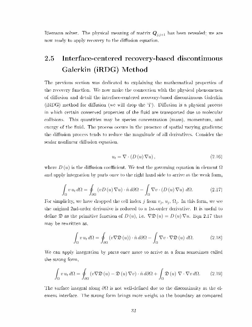
Riemann solver. The physical meaning of matrix Qj,j+1 has been revealed; we are
now ready to apply recovery to the diusion equation.
2.5 Interface-centered recovery-based discontinuous
Galerkin (iRDG) Method
The previous section was dedicated to explaining the mathematical properties of
the recovery function. We now make the connection with the physical phenomenon
of diusion and detail the interface-centered recovery-based discontinuous Galerkin
(iRDG) method for diusion (we will drop the i). Diusion is a physical process
in which certain conserved properties of the uid are transported due to molecular
collisions. This quantities may be species concentration (mass), momentum, and
energy of the uid. The process occurs in the presence of spatial varying gradients;
the diusion process tends to reduce the magnitude of all derivatives. Consider the
scalar nonlinear diusion equation,
ut = ∇ · (D (u)∇u) , (2.16)
where D (u) is the diusion coecient. We test the governing equation in element Ω
and apply integration by parts once to the right hand side to arrive at the weak form,∫Ω
v ut dΩ =
∮∂Ω
(vD (u)∇u) · n d∂Ω−∫
Ω
∇v · (D (u)∇u) dΩ. (2.17)
For simplicity, we have dropped the cell index j from vj, uj, Ωj. In this form, we see
the original 2nd-order derivative is reduced to a 1st-order derivative. It is useful to
dene D as the primitive function of D (u), i.e. ∇D (u) = D (u)∇u. Eqn 2.17 thus
may be rewritten as,∫Ω
v ut dΩ =
∮∂Ω
(v∇D (u)) · n d∂Ω−∫
Ω
∇v · ∇D (u) dΩ. (2.18)
We can apply integration by parts once more to arrive at a form sometimes called
the strong form,∫Ω
v ut dΩ =
∮∂Ω
(v∇D (u)−D (u)∇v) · n d∂Ω +
∫Ω
D (u) ∇ · ∇v dΩ. (2.19)
The surface integral along ∂Ω is not well-dened due to the discontinuity at the el-
ement interface. The strong form brings more weight to the boundary as compared
32
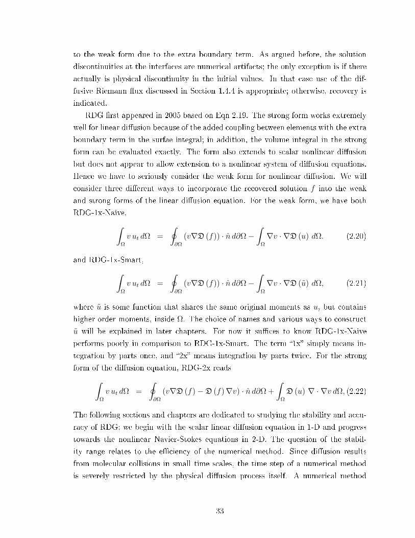
to the weak form due to the extra boundary term. As argued before, the solution
discontinuities at the interfaces are numerical artifacts; the only exception is if there
actually is physical discontinuity in the initial values. In that case use of the dif-
fusive Riemann ux discussed in Section 1.4.4 is appropriate; otherwise, recovery is
indicated.
RDG rst appeared in 2005 based on Eqn 2.19. The strong form works extremely
well for linear diusion because of the added coupling between elements with the extra
boundary term in the surfae integral; in addition, the volume integral in the strong
form can be evaluated exactly. The form also extends to scalar nonlinear diusion
but does not appear to allow extension to a nonlinear system of diusion equations.
Hence we have to seriously consider the weak form for nonlinear diusion. We will
consider three dierent ways to incorporate the recovered solution f into the weak
and strong forms of the linear diusion equation. For the weak form, we have both
RDG-1x-Naive,∫Ω
v ut dΩ =
∮∂Ω
(v∇D (f)) · n d∂Ω−∫
Ω
∇v · ∇D (u) dΩ. (2.20)
and RDG-1x-Smart,∫Ω
v ut dΩ =
∮∂Ω
(v∇D (f)) · n d∂Ω−∫
Ω
∇v · ∇D (u) dΩ, (2.21)
where u is some function that shares the same original moments as u, but contains
higher order moments, inside Ω. The choice of names and various ways to construct
u will be explained in later chapters. For now it suces to know RDG-1x-Naive
performs poorly in comparison to RDG-1x-Smart. The term 1x simply means in-
tegration by parts once, and 2x means integration by parts twice. For the strong
form of the diusion equation, RDG-2x reads∫Ω
v ut dΩ =
∮∂Ω
(v∇D (f)−D (f)∇v) · n d∂Ω +
∫Ω
D (u) ∇ · ∇v dΩ, (2.22)
The following sections and chapters are dedicated to studying the stability and accu-
racy of RDG; we begin with the scalar linear diusion equation in 1-D and progress
towards the nonlinear Navier-Stokes equations in 2-D. The question of the stabil-
ity range relates to the eciency of the numerical method. Since diusion results
from molecular collisions in small time scales, the time step of a numerical method
is severely restricted by the physical diusion process itself. A numerical method
33

should not impose a further unnecessary penalty on the time step. The study of the
accuracy of RDG includes demonstrating the improvement over existing methods,
and capturing complicated diusion-dominated phenomena such as those found in a
boundary layer. We begin our analysis with stability proofs of various RDG schemes.
2.6 Evolution of the recovery-based discontinuous
Galerkin methods
Since its inception in 2005, RDG has weathered numerous obstacles and grown into a
mature method. The rst RDG method was called RDG-2x and achieved an unsur-
passed order of accuracy for the linear diusion equation. The use of twice integrating
by parts works well on the weighted residual of the linear diusion equation because
the resulting volume integral is evaluated exactly. However, twice integrating by parts
for nonlinear diusion equations is usually implausible because the primitive in Eqn.
2.17 does not exist.
A small cottage industry slowly grew from the seeds of the recovery concept.
Marshall C. Galbraith applied a backward integration by parts on the volume integral
to obtain the RDG-3x form,∫Ωv ut dΩ =
∮∂Ω
(v∇D (f) + D (u− f)∇v) · n d∂Ω−∫
Ω∇v · ∇D (u) dΩ. (2.23)
French, Galbraith and Osorio [12] worked further with a modied RDG method using
a symmetric recovery procedure to facilitate math proofs. RDG-3x introduces addi-
tional terms and complexity into the boundary integral; hence, RDG-3x is usually
used in proofs instead of numerical calculations. Park et al. [29] were the rst to
apply the recovery concept as an solution-enhancement technique (see Section 2.8).
Solution enhancement increases the order of accuracy of a scheme without intro-
ducing additional solution coecients; this has a signicant positive impact on the
performance of DG schemes by reducing the memory burden.
Till the end of 2009, our research was focused on Fourier analysis, stability proofs
and extension to 2-D unstructured grids. RDG-1x was of direct interest due to its
shorter form; however, the accuracy of the volume integral has to be improved. In
this respect two new schemes in the RDG-1x-Smart family were introduced, RDG-
1xf and RDG-1xf . These schemes are limited in success due to instability for higher
p and added complexity on unstructured grids. In 2010 we recognized the need to
improve on the solution and the recovery function inside the volume and surface
34

integral, respectively, to accommodate the nonlinear diusion equations. The newest
scheme, RDG-1x+ and RDG-1x++, are shown to work with Navier-Stokes viscous
terms, and numerical Fourier analysis shows the two schemes are stable and extremely
accurate. The + symbol indicates the number of times that the recovery information
is reused. In RDG-1x+, the recovered function is used for the the diusion ux, and
then it is reused to enhance the solution inside the volume integral. RDG-1x++
takes it one step further by reusing the enhanced solution to obtain a new enhanced
recovered function. An experimental RDG-0x+ scheme is also introduced briey
to demonstrate the ability to discretize the PDE without any integration by parts.
RDG-0x+ achieves this by absorbing the surface integral into the volume integral,
allowing us to produce very ecient schemes. Currently the RDG-1x-Smart family
is too complicated for a general mathematical proof; as a result, we only provide
numerical evidence of stability in Chapters 3 and 4. Meanwhile, we continue with the
mathematical proofs of stability for both RDG-2x and RDG-1x-Naive.
2.7 Stability proofs for interface recovery-based dis-
continuous Galerkin methods
A popular method of studying stability of DG methods is to look at the time rate
of change of the total energy of the solution. The strategy is to show the energy is
decaying in time, or equivalently showing the RHS's of Eqns 2.20, 2.21, and 2.23 are
negative if v = u. We rst begin with the original RDG-2x method; the proof of
RDG-1x-Naive is a simplied version of RDG-2x.
2.7.1 Proof for RDG-2x
The proof rst focuses on the p ≥ 1 case, and then deals with the case p = 0, which is
dierent since the volume integral vanishes. In Eqn 2.23 we replace the test function
v by the numerical solution u, thus testing u with itself; then we integrate over the
complete computational domain V with boundary S,∫V
∂
∂t
(u2
2
)dV =
∮S
(u∇D (f)−D (f)∇u) · n dS
+
∮E
[u∇D (f)−D (f)∇u] · n dE
+
∫V
D (u) ∇ · ∇u dV . (2.24)
35

The LHS is the time rate of change of the energy of the solution, and the RHS consists
of a surface integral over the computational domain boundary S, a surface integral
over all element interfaces E , and a volume integral of the whole domain V . Note
that if the normal n is dened as pointing from element Ωj to element Ωj+1, the
jump across an interface must be dened as, [·] = (·)j − (·)j+1. We undo the second
integration by parts by performing a backward integration by parts on the the volume
integral, ∫V
∂
∂t
(u2
2
)dΩ =
∮S
(u∇D (f)−D (f)∇u) · n dS
+
∮E
[u∇D (f) + (D (u)−D (f))∇u] · n dE
−∫V∇u · ∇D (u) dV . (2.25)
The diusion coecient is not a function of mesh size, hence we assumeD (u) ∼ O (1).
There are three terms on the RHS with the third term being a volume integral that
is negative denite of O (1). The strategy is to show the rst surface integral terms,
the domain-boundary surface integral and the element-interface surface integral, are
much smaller than the volume integral. Consider a normalized physical domain where
V and S are of O (1), then E is O (h−1) where h is a typical mesh width and much
smaller than unity. It is easy to visualize the total area of the element-interfaces is
much larger than the area of the domain boundary, therefore we conclude the element-
interface surface integral is potentially much larger than the domain-boundary surface
integral. Focusing on the element-interface surface integral, we rewrite the integrand
in terms of average < · > and jump [·] notations:
[u∇D (f) + (D (u)−D (f))∇u] · n = [u]∇D (f) + [D (u)−D (f)] < ∇u > · n+
+ < D (u)−D (f) > [∇u] · n,= ([u]∇D (f) + [D (u)] < ∇u >) · n+
+ (< D (u) > −D (f)) [∇u] · n. (2.26)
Assume the initial values, of which u is the projection, are suciently smooth, say,
p + 1 times continuously dierentiable, then both [u] and < D (u) > −D (f) are of
O (hp+1), while [∇u] is O (hp) for p ≥ 1 and 0 for p = 0. Hence the two terms in
parentheses on the RHS of Eqn 2.26 are of O (hp+1) and O (h2p+1) respectively for
p ≥ 1. The rst term with O (hp+1) dominates the integrand; as a result the second
term in Eqn 2.25 is of O (hp) . For a suciently ne grid, the boundary integrals
36

becomes negligibly small compared to the negative denite volume integral.
For p = 0, ∇u = 0, so the negative-denite integral reduces to zero, and the
surface integral E assumes its role. We need to compare the magnitude of the surface
integral over S to the surface integral over E . We rst look at the magnitude of
the element-interface surface integral term. The integrand in Eqn 2.26 simplies to
[u]∇D (f) · n. In this case [u] = O (h) and the recovery procedure yields
∇D (f) · n = − [D (u)]
hcn, (2.27)
where hcn is the distance between the centroids of neighboring elements measured
along their interface-normal. The integrand becomes,
[u]∇D (f) · n = −D [u]2
hcn= −|O (h) | →
∮E
[u]∇f · n dE = − | O (1) |; (2.28)
here D = 1[u]
∫jump
D (u) du > 0. The boundary conditions are applied on the domain-
boundary surface integral. We show for both Dirichlet and Neumann boundary con-
ditions that the surface integral over S for p = 0 is still negligibly small. In the RDG
method, the boundary condition is applied on the recovery function f , not the interior
solution u. For a Dirichlet boundary condition with f = 0 on S, the integrand for
p ≥ 0 reduces to
u∇D (f) + (D (u)−D (f))∇u = (u− f)∇D (f) + (D (u)−D (f))∇u = O(hp+1
),
(2.29)
which again is small compared to terms of O (1). For an adiabatic Neumann boundary
condition with ∇D (f) · n = 0 on S, the integral is simplied to∮S
∇(u− f)2
2· n dS = O
(h2p+1
), p ≥ 0. (2.30)
Once again this term is small compared to O (1). This implies for that p ≥ 0 the
negative-denite element-interface surface integral dominates the domain-boundary
surface integral. This completes the stability proof for all p. The proof of RDG-1x
mimics the one for RDG-2x.
37
2.7.2 Proof for RDG-1x-Naive
We rst replace the test functions with the numerical solution u in Eqn 2.20 and
integrate over the complete computational domain V with boundary S,
∫V
∂
∂t
(u2
2
)dV =
∮S
(u∇D (f)) · n dS
+
∮E
[u∇D (f)] · n dE
−∫V∇u · (D (u)∇u) dV . (2.31)
The volume integral is negative denite of magnitude O (1) for p > 0. Again, we
consider a normalized physical domain where V and S are of O (1), then E is O (h−1)
where h is a number much smaller than unity. Using the same argument as for RDG-
2x, we conclude the element-interface surface integral is the largest of the two surface
integrals. We may rewrite its integrand as
[u∇D (f)] · n = [u]∇D (f) · n, (2.32)
here [u] is of magnitude O (hp+1), making the internal surface integral O (hp) for
p ≥ 1. For a suciently ne grid, both boundary integrals become negligibly small
compared to the negative denite volume integral.
For p = 0, RDG-2x is identical to RDG-1x-Naive. The proof from the previous
sections applies here; we conclude RDG-1x-Naive is energy stable for all p.
2.7.3 Note on RDG-1x-Smart
RDG-1x-Smart is a family of schemes designed to improve on the surface and vol-
ume integral in the weak form of the diusion operator. There is no stability proof
of RDG-1x-Smart due to the large number of choices for f and u; currently the
members include RDG-1xf , RDG-1xf , RDG-1x+, RDG-1x++, and RDG-1x++CO
where CO stands for Cartesian optimization. In later chapters, we use numerical
experiment and Fourier analysis to show that certain members of the smart family are
stable for various p. We believe the proof is in the pudding; the extremely high order
of accuracy is not coincidental. Research on improving RDG-1x-Smart is ongoing; a
stability proof for RDG-1x-Smart may appear in a future publication.
38
2.8 Recovery concept for solution enhancement
In this thesis, solution enhancement is dened as a process to add higher order com-
ponents to the solution. A full solution enhancement adds enough components to
raise the solution polynomial by a full order. Park et al. [29] experimented with full
solution enhancement using the recovery concept over a large stencil in cell-centered
RDG (cRDG). Since the main expense of their numerical experiments comes from
solving a large implicit system, their objective is to increase the order of the scheme
without increasing the number of solution coecients. Full solution enhancement is
extremely costly; hence, we explore cheaper ways of enhancing the solution.
We dierentiate ourselves by focusing on recovery between two cells only (binary
recovery). Binary recovery involves far fewer cells, which signicantly reduces the size
of matrix operations and allows for eective parallelization. Although binary recovery
does not provide a full solution enhancement, it does allow us to selectively choose
the correct components to add to the solution for a more accurate evaluation of the
diusion operator. As we will show later, one cannot blindly pursue a full solution
enhancement due to the rising cost in higher physical dimension; one must carefully
choose the components to enhance based on the nature of the governing equations.
39

CHAPTER III
RDG in One-Dimension for Scalar
Equation
Our research principle is to design a user-friendly DG diusion scheme which ev-
erybody can understand without a master's degree in applied mathematics. This
chapter is intended to explore and reveal the most fundamental properties of RDG
in a simple 1-D setting. Focusing on the linear diusion equation, we analyze the
scheme for linear stability and accuracy. This simple setting also provides a common
framework to compare RDG with various members of the (σ, µ)-family. Most impor-
tantly, when we rewrite RDG schemes in terms of jumps and averages of quantities
across cell interfaces, RDG schemes contain penalty-like terms previously unseen in
the (σ, µ)-family. Finally, we couple RDG with Runge-Kutta (RK) time-marching
and solve the advection-diusion and nonlinear diusion equations.
Before the show begins, we provide a list of the RDG schemes in the order of
appearance. The rst scheme is the original RDG-2x which uses twice integration by
parts on the weighted-residual formulation of the linear diusion equation and the
recovery concept for the diusion ux. We then compare RDG with the (σ, µ)-family,
which usually follow from the form once integrated by parts. On this platform we
introduce RDG-1xf which attempts to improve upon RDG-1x-Naive. Finally, we
present RDG-1x+ for nonlinear diusion. Out of the many schemes introduced in
this chapter, we focus on analysis of RDG-2x only for the following reasons. First,
numerical experiment and Fourier analysis show RDG-1xf is unstable for p ≥ 3.
Secondly, the RDG-1x+ scheme is equivalent to RDG-2x for 1-D linear diusion
equation; the analysis of RDG-2x applies directly to RDG-1x+. Lastly, RDG-1x-
Naive is not of particular interest because of its lack of accuracy.
40

3.1 1-D recovery equations for binary recovery
The basic ingredient of any RDG scheme is the recovered function based on binary re-
covery (BR). The recovered function provides an unique solution value and derivatives
at a cell interface where the solution was originally undened due to the discontinu-
ity. As the name of BR implies, only the two cells sharing one common interface are
involved. Consider the solutions in two adjacent cells of the form presented in Eqn
2.1, we look for a recovered function centered on the shared interface in the form of
Eqn 2.3. The 1-D recovery equations are∫Ωj
vjuj dx =
∫Ωj
vjfj,j+1 dx,∫Ωj+1
vj+1uj+1 dx =
∫Ωj+1
vj+1fj,j+1 dx. (3.1)
The recovered function is in a coordinate system dierent from that of the solutions
of each cell. We introduce the r-coordinate for the recovered function and the ξ-
coordinate for the local solution. The transformation between r and ξ coordinates
is strictly geometry-dependent; the details are explained below. We consider three
examples with Legendre polynomials for piecewise-constant (p = 0), piecewise-linear
(p = 1) and piecewise-quadratic (p = 2) solutions on an uniform grid.
3.1.1 Piecewise-constant (p = 0) recovery
A DG scheme with p = 0 is equivalent to a nite-volume scheme. Let the test space
V be equal to the solution space U , and be spanned by the following basis function,
v0 = 1, ξ ∈ [0, 1] , (3.2)
where ξ is the local coordinate, and the solution in Ωj be expressed as
uj = a0,jv0,j = a0,j. (3.3)
Here, a0 can be viewed as the cell average. We look for a recovered function between
Ωj and Ωj+1 of the form,
fj,j+1 (r) = b0 + b1r, r ∈ [−1, 1], (3.4)
41

such that Ωj belongs to r ∈ [−1, 0] and Ωj+1 belongs to r ∈ [0, 1] (see Figure 3.1).
The transformation of variable is given by
r = ξ − 1, for Ωj, (3.5)
r = ξ − 0, for Ωj+1. (3.6)
r
ξ ξ0 1 0 1
0 1-1
Ω Ωj j+1
Figure 3.1: The recovery coordinate system spans the union of two neighboring cells,while each cell has a local coordinate ξ.
Note that r = 0 is centered on the interface shared by Ωj and Ωj+1. Eqn 3.1 is
rewritten into matrix-vector form after performing the necessary integrations,(1 0
0 1
)(a0,j
a0,j+1
)=
(1 −1
2
1 12
)(b0
b1
)j,j+1
. (3.7)
Solving for bi gives, (b0
b1
)j,j+1
=
(a0,j+a0,j+1
2
−a0,j + a0,j+1
). (3.8)
3.1.2 Piecewise-linear (p = 1) recovery
Let the test space V be equal to the solution space U , and be spanned by the following
basis functions,
v0 = 1, v1 = 2ξ − 1, ξ ∈ [0, 1] , (3.9)
where ξ is the local coordinate, and the solution in Ωj be expressed as,
uj = a0,jv0,j + a1,jv1,j. (3.10)
We look for a recovered function between Ωj and Ωj+1 of the form,
fj,j+1 (r) = b0 + b1r + b2r2 + b3r
3, r ∈ [−1, 1], (3.11)
42

such that Ωj belongs to r ∈ [−1, 0] and Ωj+1 belongs to r ∈ [0, 1]. Using the same
variable transformation as the previous section, Eqn 3.1 is rewritten into matrix-
vector form after performing the necessary integrations,1 0 0 0
0 13
0 0
0 0 1 0
0 0 0 13
a0,j
a1,j
a0,j+1
a1,j+1
=
1 −1
213−1
4
0 16−1
6320
1 12
13
14
0 16
16
320
b0
b1
b2
b3
j,j+1
. (3.12)
Solving for bi gives,b0
b1
b2
b3
j,j+1
=
a0,j+a0,j+1
2+
a1,j−a1,j+1
39(a0,j+1−a0,j)
4− 5(a1,j+a1,j+1)
4
a1,j+1 − a1,j
5(a0,j+1−a0,j)
2+
5(a1,j+a1,j+1)
2
. (3.13)
3.1.3 Piecewise-quadratic (p = 2) recovery
Let the test space V be equal to the solution space U , and be spanned by the following
basis functions,
v0 = 1, v1 = 2ξ − 1, v2 = 6ξ2 − 6ξ + 1, ξ ∈ [0, 1] , (3.14)
where ξ is the local coordinate, and the solution in Ωj be expressed as,
uj = a0,jv0,j + a1,jv1,j + a2,jv2,j. (3.15)
We look for a recovered function between Ωj and Ωj+1 of the form,
fj,j+1 (r) = b0 + b1r + b2r2 + b3r
3 + b4r4 + b5r
5, r ∈ [−1, 1]. (3.16)
43

The resulting system in matrix-vector form looks like
1 0 0 0 0 0
0 13
0 0 0 0
0 0 15
0 0 0
0 0 0 1 0 0
0 0 0 0 13
0
0 0 0 0 0 15
a0,j
a1,j
a2,j
a0,j+1
a1,j+1
a2,j+1
=
1 −12
13−1
415
−16
0 16−1
6320
− 215
542
0 0 130− 1
20235
− 584
1 12
13
14
15
16
0 16
16
320
215
542
0 0 130
120
235
584
b0
b1
b2
b3
b4
b5
j,j+1
,
(3.17)
with solution
b0
b1
b2
b3
b4
b5
j,j+1
=
a0,j+a0,j+1
2+
13(a1,j−a1,j+1)
32+
7(a2,j+a2,j+1)
3215(−a0,j+a0,j+1)
4− 11(a1,j+a1,j+1)
4+
6(−a2,j+a2,j+1)
3215(−a1,j+a1,j+1)
8− 21(a2,j+a2,j+1)
825(a0,j−a0,j+1)
2+
25(a1,j+a1,j+1)
2+ 8 (a2,j − a2,j+1)
35(a1,j−a1,j+1)
32+
105(a2,j+a2,j+1)
3221(−a0,j+a0,j+1)
2+
21(a1,j+a1,j+1)
2+
42(−a2,j+a2,j+1)
5
. (3.18)
3.2 RDG-2x for linear diusion
The original RDG-2x is applied to the spatial derivatives on the RHS of the linear dif-
fusion equation, while the temporal derivative is handled by an explicit time-marching
Runge-Kutta (RK) scheme. This section demonstrates the discretization of the RHS
of the linear diusion equation with RDG-2x for p = 0, 1 and 2. The recovered
function is used as the ux component in the RDG-2x scheme,∫Ωj
vut dx = D [vfx − vxf ]j+ 1
2
j− 12
+D
∫Ωj
vxxu dx, (3.19)
where the solution u is replaced with the smooth recovered function f in the surface
integral. In 1-D the surface integrals reduce to point values of f and fx at the interface.
However, the update equation is given in terms the global spatial coordinate x; it is
necessary to convert the global coordinate into local coordinate for a DG scheme.
The transformation between ξ and x is given by dξdx
= 1∆x
; the update equation in
terms of ξ is then
∆x
∫Ωj
vut dξ =D
∆x[vfξ − vξf ]
j+ 12
j− 12
+D
∆x
∫Ωj
vξξu dξ. (3.20)
44

Recall that f uses a dierent coordinate system, where the transformation from r
to ξ is conveniently given by drdξ
= 1, hence fξ = fr. Upon inserting the recovered
functions from the previous section, we obtain the update matrix for each cell Ωj.
Update scheme for RDG-2x (p = 0)
With only one basis function, v0 = 1, the update equation reduces to
d
dt
(a0j
)∆x =
D
∆x[fξ]
j+ 12
j− 12
=D
∆x
[(fξ)j,j+1 − (fξ)j−1,j
], (3.21)
where the rst derivative of recovered function evaluates to
(fr (0))j,j+1 = (b1)j,j+1 = −a0,j + a0,j+1, (3.22)
(fr (0))j−1,j = (b1)j,j+1 = −a0,j−1 + a0,j. (3.23)
The nal update scheme becomes,
d
dt
(a0j
)=
D
∆x2(a0,j+1 − 2a0,j + a0,j−1) .
=D
∆x2([1] [−2] [1])
a0,j−1
a0,j
a0,j+1
. (3.24)
Indeed the RDG-2x scheme for p = 0 reduces to the central dierence scheme which
is 2nd-order accurate in space, and the only consistent scheme for p = 0. Although
the p = 0 case is not of interest in the DG framework, it is still satisfying to show the
RDG-2x scheme comes from a very good pedigree. Note that the update equation is
rewritten into matrix-vector form which will come in handy in a later section.
Update scheme for RDG-2x (p = 1)
Using the linear basis functions v0 = 1 and v1 = 2ξ−1, the update equations become
d
dt
(a0ja1j
3
)=
D
∆x2
((fξ)j,j+1 − (fξ)j−1,j(
(fξ)j,j+1 + (fξ)j−1,j
)− 2 (fj,j+1 − fj−1,j)
). (3.25)
45
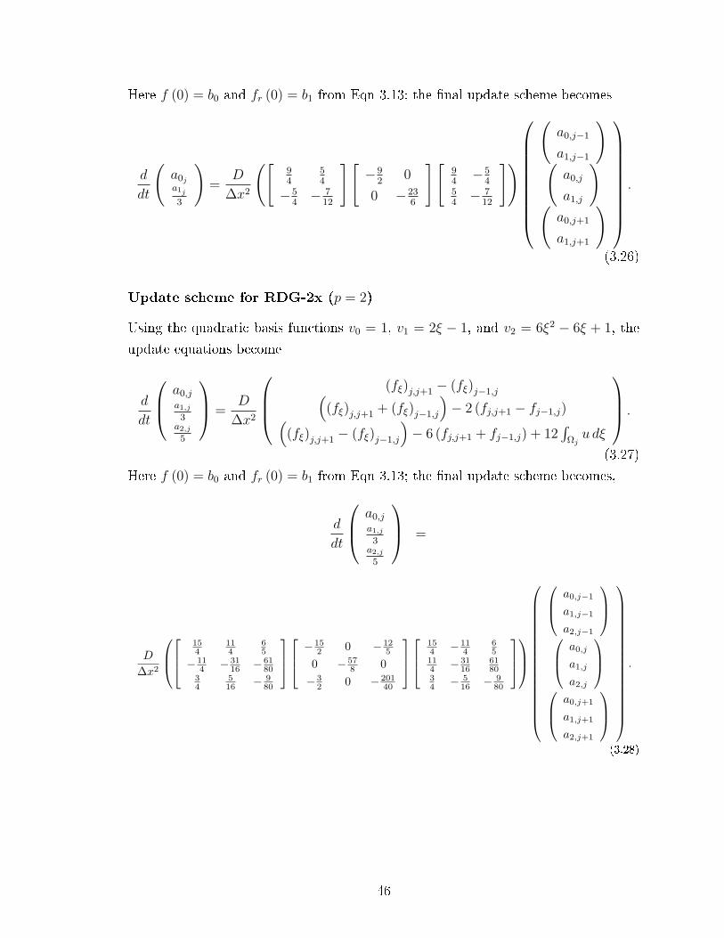
Here f (0) = b0 and fr (0) = b1 from Eqn 3.13; the nal update scheme becomes
d
dt
(a0ja1j
3
)=
D
∆x2
([94
54
−54− 7
12
][−9
20
0 −236
][94−5
454− 7
12
])
(a0,j−1
a1,j−1
)(a0,j
a1,j
)(a0,j+1
a1,j+1
)
.
(3.26)
Update scheme for RDG-2x (p = 2)
Using the quadratic basis functions v0 = 1, v1 = 2ξ − 1, and v2 = 6ξ2 − 6ξ + 1, the
update equations become
d
dt
a0,j
a1,j
3a2,j
5
=D
∆x2
(fξ)j,j+1 − (fξ)j−1,j(
(fξ)j,j+1 + (fξ)j−1,j
)− 2 (fj,j+1 − fj−1,j)(
(fξ)j,j+1 − (fξ)j−1,j
)− 6 (fj,j+1 + fj−1,j) + 12
∫Ωju dξ
.
(3.27)
Here f (0) = b0 and fr (0) = b1 from Eqn 3.13; the nal update scheme becomes,
d
dt
a0,j
a1,j
3a2,j
5
=
D
∆x2
154
114
65
− 114 − 31
16 − 6180
34
516 − 9
80
−
152 0 − 12
5
0 − 578 0
− 32 0 − 201
40
154 − 11
465
114 − 31
166180
34 − 5
16 − 980
a0,j−1
a1,j−1
a2,j−1
a0,j
a1,j
a2,j
a0,j+1
a1,j+1
a2,j+1
.
(3.28)
46

3.3 Fourier analysis and eigenvectors
As Professor David Gottlieb famously noted, we can always analyze a 1-D system to
death, which in scientic language means a very complete analysis can be performed
on a simple system of equations. We use Fourier analysis to reveal the order of
accuracy and stability limit of RDG schemes for the linear diusion equation. The
key components in our Fourier analysis is to identify the eigenvalues and eigenvectors.
We begin by giving an overview of the steps involved in the Fourier analysis, and
explaining the physical meaning behind the eigenvalues and eigenvectors.
Our Fourier analysis is based on the scalar linear diusion equation,
ut = Duxx, (3.29)
where D is a positive constant. The weighted-residual formulation after once integra-
tion by parts becomes,∫Ω
vut dx = D
∮∂Ω
vux d∂Ω−D∫
Ω
vxux dx, (3.30)
or twice integrated by parts,∫Ω
vut dx = D
∮∂Ω
(vux − vxu) d∂Ω +D
∫Ω
vxxu dx. (3.31)
Note we dropped the cell index from v and u for simplicity. We obtain RDG-2x by
replacing the solution u in the surface integral with the recovered function f ,∫Ω
vut dx = D
∮∂Ω
(vfx − vxf) d∂Ω +D
∫Ω
vxxu dx. (3.32)
Our next step is to rewrite the RHS of Eqn 3.32 as a discrete Fourier operator and
compare the result with the exact Fourier operator. Fourier operators are expressed
in terms of the Fourier mode, β. The solution in cells adjacent to Ωj is related through
the Fourier mode,
uj+k = eiβkuj = T kuj, (3.33)
where T k is the translation operator and uj is a vector of solution coecients. The
RHS of Eqn 3.32 is simply expressed as,
1
D
∂
∂tuj = M (β) uj, (3.34)
47

whereM (β) is a matrix representing the discrete Fourier operator. The exact Fourier
symbols for 1st and 2nd-order spatial dierentiations are
∂
∂x=
iβ
∆x, (3.35)
∂2
∂x2= − β2
∆x2, (3.36)
respectively; hence, the exact Fourier operator for the 2nd-order diusion equation is
M (β) = −Dβ2I, (3.37)
where I is the identity matrix. A comparison of the eigenvalues of the discrete Fourier
operator with the exact Fourier operator reveals the level of accuracy at which the
numerical scheme approximates the diusion operator. The signs of the eigenvalues
also dictate the stability of a scheme; in this case, a positive eigenvalue indicates
instability. However, the eigenvalues only allow us to determine the stability range
and the evolution error. The other issue of crucial concern is the initial projection
error, which is a measure of the scheme's ability to preserve a smooth solution. The
projection error is determined from the eigenvectors of M (β). We are now ready for
some Fourier analysis.
3.3.1 RDG-2x Fourier analysis: piecewise-linear (p = 1)
Consider a numerical solution expanded in terms of a solution vector ~uj and the
piecewise-linear Legendre basis functions in the local spatial coordinate,
~uj =
(uj
∆uj
), (3.38)
uj = uj + ∆uj (2ξ − 1) , ξ ∈ [0, 1] , (3.39)
The complete update scheme with RDG for solving Eqn 3.32 is given by,
∂
∂t
(uj
∆uj
)=
D
∆x2
( [94
54
−154−7
4
] [−9
20
0 −232
] [94−5
4154−7
4
] ) T−1 (~uj)
I (~uj)
T+1 (~uj)
.
(3.40)
48

Note this is very similar to Eqn. 3.26, except T k is the translation operator such that
T+1 (~uj) = ~uj+1, (3.41)
I (~uj) = ~uj, (3.42)
T−1 (~uj) = ~uj−1, (3.43)
where j is a spatial index, and I is the identity operator. We convert the translation
operators into Fourier modes via
T±j = e±i β j = cos (jβ)± i sin (jβ) , (3.44)
and arrive at the following form,
∂
∂x
(uj
∆uj
)=
D
∆x2
(−9
2(1− cosβ) −5
2i sinβ
152i sinβ −1
2(23 + 7cosβ)
)(uj
∆uj
)(3.45)
= MRDG-2x,p1 (β)
(uj
∆uj
). (3.46)
The two eigenvalues of MRDG-2x,p1 are given by,
λ1,2 = −8 +cosβ
2±√
118 + 112cosβ + (cosβ)2 − 6cos2β, (3.47)
and then Taylor-expanding the eigenvalues for small β reveals,
λ1 = −β2 +β6
360+O
(β8), (3.48)
λ2 = −15 +β2
2+β4
24− β6
240+O
(β8). (3.49)
The left side of Figure 3.2 shows the two eigenvalues attempting to represent the
diusion operator with the curve λ = −β2. By convention, the order of accuracy of
a scheme usually refers to the eigenvalues for small β, or low frequency data. The
contribution of high frequency data to the diusion operator is less signicant (they
are also known as noise). The evolution error is determined from the good eigenvalue
λ1, such that λerror = |λ1 + β2|. We dene the order of accuracy of a scheme to be,
O.O.A. = λerrorβ2 . In this case, the order of accuracy RDG-2x (p = 1) is four. Notice
the rst eigenvalue approximates the curve λ = −β2 until β = π, and then the second
eigenvalue takes over. This observation leads to the discovery of important passive
49

elements of DG schemes. DG schemes inherently contain switches which turn on and
o eigenvalues to maximize the accuracy in representing the solution. The switches
are not engineered, but possibly nature's way of dealing with sub-grid information in
an element. The study of these switches is done by analyzing the contribution from
each of the eigenvectors.
0 Π
2Π
3 Π
2
2 Π
-14
-12
-10
-8
-6
-4
-2
0
Β
Λ1,
2
0 Π
2Π
3 Π
2
2 Π
0.0
0.5
1.0
Β
C1,C
2
C1
C2
Λ1
Λ2
Figure 3.2: Eigenvalues of RDG-2x (p = 1) are shown on the left. The switch func-tions are shown on the right demonstrating the contribution of each eigen-function for various β.
Consider the initial value of the solution to be consisted of Fourier modes,
U (x) = U0eiβx∆x , (3.50)
then the initial discretization in each element Ωj is given by
uj =
∫Ωjv0U dx∫
Ωjv2
0 dx=
2sin(β2
)β
U0, (3.51)
∆uj =
∫Ωjv1U dx∫
Ωjv2
1 dx= −6i
(βcos
(β2
)− 2sin
(β2
))β2
U0. (3.52)
The general strategy of this analysis is to feed waves of dierent Fourier modes β into
the RDG diusion operator, and observe how well the RDG operator preserves the
50
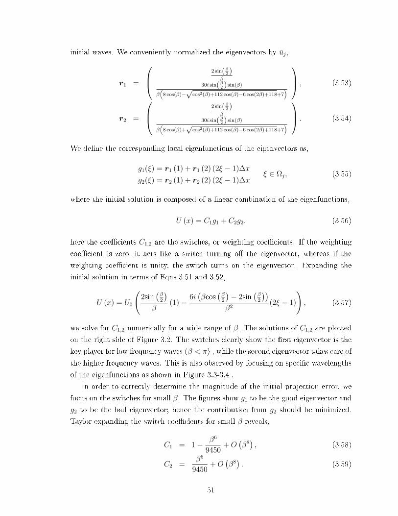
initial waves. We conveniently normalized the eigenvectors by uj,
r1 =
2 sin(β2 )β
30i sin(β2 ) sin(β)
β(
8 cos(β)−√
cos2(β)+112 cos(β)−6 cos(2β)+118+7) , (3.53)
r2 =
2 sin(β2 )β
30i sin(β2 ) sin(β)
β(
8 cos(β)+√
cos2(β)+112 cos(β)−6 cos(2β)+118+7) . (3.54)
We dene the corresponding local eigenfunctions of the eigenvectors as,
g1(ξ) = r1 (1) + r1 (2) (2ξ − 1)∆x
g2(ξ) = r2 (1) + r2 (2) (2ξ − 1)∆xξ ∈ Ωj, (3.55)
where the initial solution is composed of a linear combination of the eigenfunctions,
U (x) = C1g1 + C2g2. (3.56)
here the coecients C1,2 are the switches, or weighting coecients. If the weighting
coecient is zero, it acts like a switch turning o the eigenvector, whereas if the
weighting coecient is unity, the switch turns on the eigenvector. Expanding the
initial solution in terms of Eqns 3.51 and 3.52,
U (x) = U0
(2sin
(β2
)β
(1)− 6i(βcos
(β2
)− 2sin
(β2
))β2
(2ξ − 1)
), (3.57)
we solve for C1,2 numerically for a wide range of β. The solutions of C1,2 are plotted
on the right side of Figure 3.2. The switches clearly show the rst eigenvector is the
key player for low frequency waves (β < π) , while the second eigenvector takes care of
the higher frequency waves. This is also observed by focusing on specic wavelengths
of the eigenfunctions as shown in Figure 3.3-3.4 .
In order to correctly determine the magnitude of the initial projection error, we
focus on the switches for small β. The gures show g1 to be the good eigenvector and
g2 to be the bad eigenvector; hence the contribution from g2 should be minimized.
Taylor expanding the switch coecients for small β reveals,
C1 = 1− β6
9450+O
(β8), (3.58)
C2 =β6
9450+O
(β8). (3.59)
51

Β=Π
5
0 2 4 6 8 10-1.0
-0.5
0.0
0.5
1.0
x
Dx
g 1
0 2 4 6 8 10
-5
0
5
x
Dx
g 2
Β=2 Π
3
0.0 0.5 1.0 1.5 2.0 2.5 3.0-1.0
-0.5
0.0
0.5
1.0
x
Dx
g 1
0.0 0.5 1.0 1.5 2.0 2.5 3.0
-1.0
-0.5
0.0
0.5
1.0
1.5
2.0
x
Dx
g 2
Β=99 Π
100
0.0 0.5 1.0 1.5 2.0
-5
0
5
x
Dx
g 1
0.0 0.5 1.0 1.5 2.0-1.0
-0.5
0.0
0.5
1.0
x
Dx
g 2
Figure 3.3: Eigenfunctions of RDG-2x (p = 1) for β between π5and 99π
100. Notice the
change in scaling of both x-axis and g-axis. The dashed line representsthe analytical wave.
52
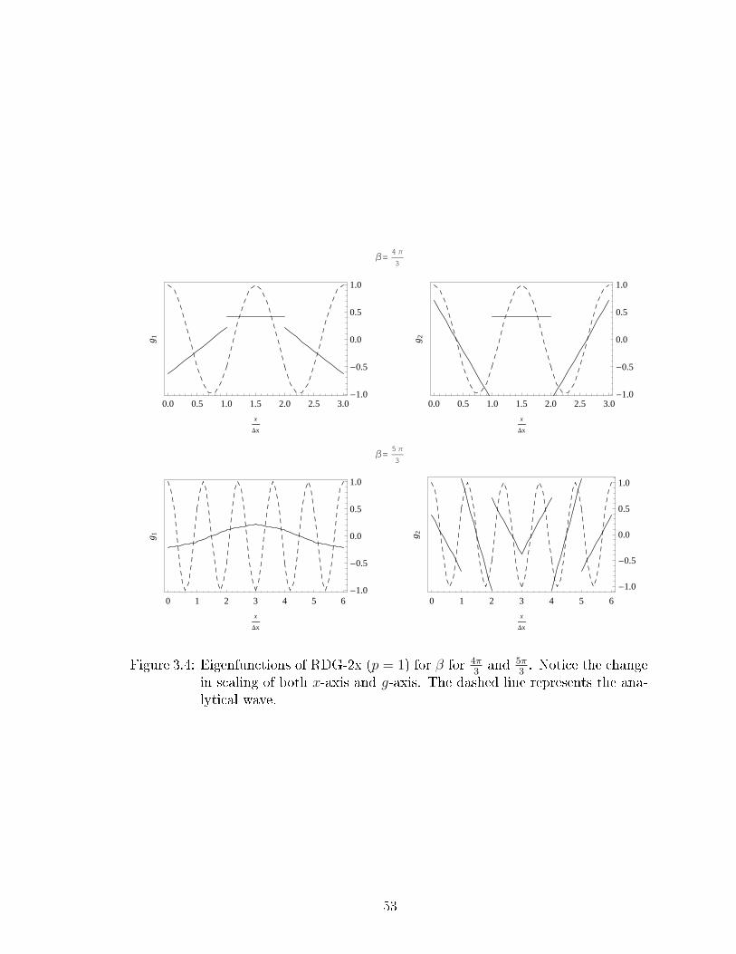
Β=4 Π
3
0.0 0.5 1.0 1.5 2.0 2.5 3.0-1.0
-0.5
0.0
0.5
1.0
x
Dx
g 1
0.0 0.5 1.0 1.5 2.0 2.5 3.0-1.0
-0.5
0.0
0.5
1.0
x
Dx
g 2
Β=5 Π
3
0 1 2 3 4 5 6-1.0
-0.5
0.0
0.5
1.0
x
Dx
g 1
0 1 2 3 4 5 6
-1.0
-0.5
0.0
0.5
1.0
x
Dx
g 2
Figure 3.4: Eigenfunctions of RDG-2x (p = 1) for β for 4π3and 5π
3. Notice the change
in scaling of both x-axis and g-axis. The dashed line represents the ana-lytical wave.
53
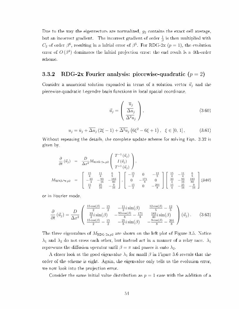
Due to the way the eigenvectors are normalized, g2 contains the exact cell average,
but an incorrect gradient. The incorrect gradient of order 1βis then multiplied with
C2 of order β6, resulting in a initial error of β5. For RDG-2x (p = 1), the evolution
error of O (β4) dominates the initial projection error; the end result is a 4th-order
scheme.
3.3.2 RDG-2x Fourier analysis: piecewise-quadratic (p = 2)
Consider a numerical solution expanded in terms of a solution vector ~uj and the
piecewise-quadratic Legendre basis functions in local spatial coordinate,
~uj =
uj
∆uj
∆2uj
, (3.60)
uj = uj + ∆uj (2ξ − 1) + ∆2uj(6ξ2 − 6ξ + 1
), ξ ∈ [0, 1] , (3.61)
Without repeating the details, the complete update scheme for solving Eqn. 3.32 isgiven by,
∂
∂t(~uj) =
D
∆x2MRDG-2x,p2
T−1 (~uj)I (~uj)T+1 (~uj)
,
MRDG-2x,p2 =
154
114
65
− 334 − 93
16 − 18380
154
2516 − 9
16
, −
152 0 − 12
5
0 − 1718 0
− 152 0 − 201
8
154 − 11
465
334 − 93
1618380
154 − 25
16 − 916
,(3.62)or in Fourier mode,
∂
∂t(~uj) =
D
∆x2
15 cos(β)
2− 15
2−11
2i sin(β) 12 cos(β)
5− 12
5332i sin(β) −93 cos(β)
8− 171
818340i sin(β)
15 cos(β)2− 15
2−25
8i sin(β) −9 cos(β)
8− 201
8
(~uj) . (3.63)
The three eigenvalues of MRDG-2x,p2 are shown on the left plot of Figure 3.5. Notice
λ1 and λ2 do not cross each other, but instead act in a manner of a relay race. λ1
represents the diusion operator until β = π and passes it onto λ2.
A closer look at the good eigenvalue λ1 for small β in Figure 3.6 reveals that the
order of the scheme is eight. Again, the eigenvalue only tells us the evolution error,
we now look into the projection error.
Consider the same initial value distribution as p = 1 case with the addition of a
54

0 Π
2Π
3 Π
2
2 Π
-30
-25
-20
-15
-10
-5
0
Β
Λ1,
2,3
0 Π
2Π
3 Π
2
2 Π
0.0
0.2
0.4
0.6
0.8
1.0
Β
C1,C
2,C
3
Λ3
Λ2
Λ1
C3
C2
C1
Figure 3.5: Eigenvalues of RDG-2x (p = 2), are shown on the left. The switch func-tions are shown on the right demonstrating the contribution of each eigen-function for various β.
π
8
π
4
3 π
8
π
2
5.46 x 10⁻⁷
5.48 x 10⁻⁷
5.5 x 10⁻⁷
5.52 x 10⁻⁷
5.54 x 10⁻⁷
5.56 x 10⁻⁷
β
β2
+λ1
β10
Figure 3.6: A closer look at the good eigenvalue of RDG-2x (p = 2), for small β. Thedierence between the good eigenvalue and the exact diusion operatoris of order β10, implying the evolution error of the scheme is 8th-order.
second gradient,
∆2uj =
∫Ωjv2U dx∫
Ωjv2
2 dx=
10((β2 − 12) sin
(β2
)+ 6β cos
(β2
))β3
U0. (3.64)
The eigenvectors r1, r2, r3 are too complicated to be presented in analytic form. We
dene the corresponding local eigenfunctions of the eigenvectors as
g1(ξ) = r1 (1) v0 + r1 (2) v1∆x+ +r1 (2) v2∆x2
g2(ξ) = r2 (1) v0 + r2 (2) v1∆x+ +r2 (2) v2∆x2
g2(ξ) = r3 (1) v0 + r3 (2) v1∆x+ +r3 (2) v2∆x2
ξ ∈ Ωj, (3.65)
55

where the initial solution is composed of a linear combination of the eigenfunctions,
U (x) = C1g1 + C2g2 + C3g3. (3.66)
We rst acquire r1, r2, r3 numerically for xed β, and then solve for the switches
C1,2,3. The right plot of Figure 3.5 shows the switches in action for various values
of β. Figure 3.7 shows the structure of the three eigenfunctions for dierent Fourier
modes.
The gures show that g1 is the good eigenvector for small β. We look for the
contribution of the bad eigenvectors by determining the magnitude of C2 and C3.
Figure 3.8 shows that both C2 and C3 are of order β8. This is already puzzling: we
would not expect the scheme to be 8th-order accurate with such projection errors,
but numerical results suggest it is. In order to determine the full magnitude of the
projection error, we also need to know the error in the average rst and second
gradients of g1 as a function of β. We have not pursued this; the question of the
projection error of RDG-2x for p ≥ 2 is a subject for furture research.
Fourier analysis paints an interesting picture of the inner workings of RDG-2x.
As we can observe already, the complexity of the analysis for piecewise-quadratic is
quite cumbersome; therefore, we proceed no further with higher p. Next, we perform
Fourier analysis for various penalty methods and compare them with the results for
the RDG-2x scheme.
3.3.3 The venerable (σ, µ)-family Fourier analysis for p = 1
This section takes us all the way back to 1982 when Arnold introduced the rst
successful discretization of the DG diusion operator with the interior penalty method
(IPM). Van Raalte (2005) put the penalty schemes into a two-parameter family, called
the (σ, µ)-family, but did not go beyond the traditional pairs of values. Van Leer [42]
was the rst to explore the entire family for p = 1. Our immediate goal is to highlight
the dierence between RDG-2x and the (σ, µ)-family through Fourier analysis. We
then explore the (σ, µ)-plane for worthy schemes which were previously undiscovered.
56

Β=Π
5
0 2 4 6 8 10-1.0
-0.5
0.0
0.5
1.0
x
Dx
g 1
0 2 4 6 8 10
-20
-10
0
10
20
x
Dx
g 2
0 2 4 6 8 10
-5
0
5
10
x
Dx
g 3
Β=2 Π
3
0.0 0.5 1.0 1.5 2.0 2.5 3.0-1.0
-0.5
0.0
0.5
1.0
x
Dx
g 1
0.0 0.5 1.0 1.5 2.0 2.5 3.0
-2
-1
0
1
x
Dx
g 2
0.0 0.5 1.0 1.5 2.0 2.5 3.0
-3
-2
-1
0
1
2
3
x
Dx
g 3
Β=99 Π
100
0.0 0.5 1.0 1.5 2.0
-1.5
-1.0
-0.5
0.0
0.5
1.0
1.5
x
Dx
g 1
0.0 0.5 1.0 1.5 2.0-1.0
-0.5
0.0
0.5
1.0
x
Dx
g 2
0.0 0.5 1.0 1.5 2.0-1.0
-0.5
0.0
0.5
1.0
x
Dx
g 3Β=
4 Π
3
0.0 0.5 1.0 1.5 2.0 2.5 3.0-1.0
-0.5
0.0
0.5
1.0
x
Dx
g 1
0.0 0.5 1.0 1.5 2.0 2.5 3.0-1.0
-0.5
0.0
0.5
1.0
x
Dx
g 2
0.0 0.5 1.0 1.5 2.0 2.5 3.0-1.0
-0.5
0.0
0.5
1.0
x
Dx
g 3
Β=5 Π
3
0 1 2 3 4 5 6-1.0
-0.5
0.0
0.5
1.0
x
Dx
g 1
0 1 2 3 4 5 6-1.0
-0.5
0.0
0.5
1.0
x
Dx
g 2
0 1 2 3 4 5 6-1.0
-0.5
0.0
0.5
1.0
x
Dx
g 3
Figure 3.7: Eigenfunctions of RDG-2x (p = 2) for β between π5and 5π
3. Notice the
change in scaling of both x-axis and g-axis. The dashed line representsthe analytical wave.
57

0 0.1 0.2 0.3-3. ´ 10-6
-2. ´ 10-6
-1. ´ 10-6
0
1. ´ 10-6
2. ´ 10-6
3. ´ 10-6
Β
C1
Β8
,C2
Β8
Figure 3.8: For small β, C1 and C2 are the weighting coecients of the bad eigen-vectors. They scale with β8. However, no solid conclusion can be drawnfrom this analysis due to the lack of analytical formulas.
The (σ, µ)-family for the linear diusion equation is given by,∫Ωj
vut dx = −D(〈ux〉 [v] |j+ 1
2+ 〈ux〉 [v] |j− 1
2
)−D
∫Ωj
vxux dx
+ σD(〈vx〉 [u] |j+ 1
2+ 〈vx〉 [u] |j− 1
2
)− µD
∆x
([v][u] |j+ 1
2−[v][u] |j− 1
2
), (3.67)
where < . > is the average operator across an interface, and [ . ] is the dierence
operator across an interface from the right to the left. There is a distinct dierence
between applying these operators to u and v. When applied to the solution, u is taken
globally such that the value on each side of the interface comes from the two cells
sharing the interface, providing the necessary coupling between cells. When applied
to the test function, v is taken locally such that the value outside the cell is always
zero. Term 1 on the RHS is needed to achieve consistency for p > 0. For example, if
p = 1, term 1 becomes,
D(< ux >|j+ 1
2− < ux >|j− 1
2
). (3.68)
For smooth problems, this may appear to be a good approximation for the diusion
ux, but it ignores the jump in the solution. Picture two abutting elements with
dierent piecewise-constant solution; term 1 always evaluate to zero because the av-
erage gradient is zero. But the physics of diusion should induce a ux from high to
low! Term 1 and term 2 together yield an inconsistent scheme. Term 3 is a penalty
term with coecient σ. With the choice of σ = −1, terms 1 to 3 form a symmetric
operator; however, stability is not guaranteed. Term 4 is the interior penalty term
58
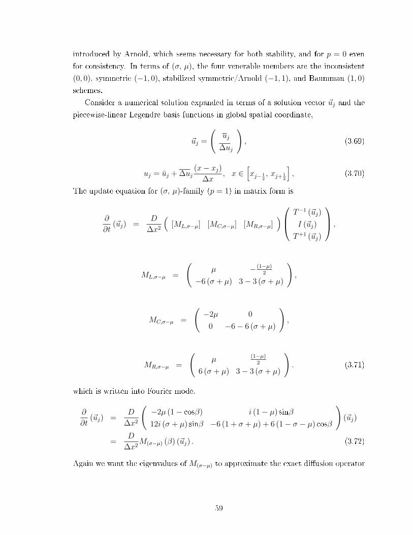
introduced by Arnold, which seems necessary for both stability, and for p = 0 even
for consistency. In terms of (σ, µ), the four venerable members are the inconsistent
(0, 0), symmetric (−1, 0), stabilized symmetric/Arnold (−1, 1), and Baumman (1, 0)
schemes.
Consider a numerical solution expanded in terms of a solution vector ~uj and the
piecewise-linear Legendre basis functions in global spatial coordinate,
~uj =
(uj
∆uj
), (3.69)
uj = uj + ∆uj(x− xj)
∆x, x ∈
[xj− 1
2, xj+ 1
2
], (3.70)
The update equation for (σ, µ)-family (p = 1) in matrix form is
∂
∂t(~uj) =
D
∆x2
([ML,σ−µ] [MC,σ−µ] [MR,σ−µ]
) T−1 (~uj)
I (~uj)
T+1 (~uj)
,
ML,σ−µ =
(µ − (1−µ)
2
−6 (σ + µ) 3− 3 (σ + µ)
),
MC,σ−µ =
(−2µ 0
0 −6− 6 (σ + µ)
),
MR,σ−µ =
(µ (1−µ)
2
6 (σ + µ) 3− 3 (σ + µ)
). (3.71)
which is written into Fourier mode,
∂
∂t(~uj) =
D
∆x2
(−2µ (1− cosβ) i (1− µ) sinβ
12i (σ + µ) sinβ −6 (1 + σ + µ) + 6 (1− σ − µ) cosβ
)(~uj)
=D
∆x2M(σ−µ) (β) (~uj) . (3.72)
Again we want the eigenvalues of M(σ−µ) to approximate the exact diusion operator
59

in Eqn 3.37. The eigenvalues are found in the following form,
λ1 = Cλ10 + Cλ1
2 β2 + Cλ14 β4 + Cλ1
6 β6 +O(β8), (3.73)
λ2 = Cλ20 + Cλ2
2 β2 + Cλ24 β4 + Cλ2
6 β6 +O(β8). (3.74)
where all the coecients, Cλj = Cλ
j (σ, µ), are dependent on σ and µ. Notice there
are no odd-order exponents in the coecients of the eigenvalues. The coecients Cλj
are found with Mathematica, and they are too complicated to be revealed. Table 3.2
provides the order of accuracy of various (σ, µ)-schemes based on the rst eigenvalue.
Recall from the previous section that the two eigenvalues play dierent roles depend-
ing on the frequency; λ1 approximates the exact spatial operator in the low frequency
range, while λ2 approximates of the spatial operator in the high frequency range.
The (σ, µ) playing eld
Our analysis of the (σ, µ)-family is summarized on the map of the σ − µ plane in
Figure 3.9. Six lines of importance are drawn, their equations are:
σ + µ = 0, (3.75)
σ + µ =5
2, (3.76)
σ − µ = −2, (3.77)
σ + µ = 1, (3.78)
µ = 1, (3.79)
µ = 0. (3.80)
The rst line, σ + µ = 0, is the line of separation between stable and unstable
domains. The domain above the line is stable, while the region below is unstable. On
the line specically, µ ≥ 0 is stable and µ < 0 is unstable. Stability comes from both
eigenvalues in Eqn 3.74 being negative, e.g. Cλ1,2
0 ≤ 0 only, and the other coecients
are ignored because they are multiplied with higher even powers of small β. Assuming
σ + µ 6= 0, the eigenvalues of M(σ−µ) are
λ1 = −β2 +O(β4), (3.81)
λ2 = −12 (σ + µ) +O(β2). (3.82)
λ1 is always negative; on the other hand, we must enforce the following condition to
60

σ+μ=0inconsistent
σ+μ=5/2
gradient consistent
μ-σ=2
λ1 4th
-ord
erStable Domain
UnstableDomain
EcientDomain
μ=1
gradient decoupling
undamped mode
μ=0
σ+μ=1
optimal eciency
BR2 (-1,3)
I (0,0) Baumann (1,0)S (-1,0)
RDG-1x (¼ , 9⁄4)
(-½ , 3⁄2)
SA (-1,1)
Figure 3.9: A intuitive map of the (σ, µ)-family. The symbols are dened as follow:S is the symmetric scheme, SA is the symmetric/Arnold scheme, Iis the inconsistent scheme, BR2 is Bassi-Rebay 2. The dark regionindicates instability, the light gray region represents ecient and stableschemes with the largest Von Neumann number (VNN), and the whiteregion designates the stable domain.
61

ensure λ2 is negative,
σ + µ > 0. (3.83)
In the case where σ + µ = 0, the eigenvalues of M(σ−µ) become
λ1 = −2µ (1− cosβ) , (3.84)
λ2 = −6 (1− cosβ) . (3.85)
It is clear from λ1 that the scheme will be stable if µ ≥ 0, and this is the reason why
schemes below µ = 0 on the line σ + µ = 0 are unstable.
The second line, σ − µ = −2, is locus of 4th-order schemes determined from
looking at the error of λ1, λerror = |λ1 + β2|. We dene the order of accuracy of a
scheme to be O.O.A. = λerrorβ2 . First, we look for 2nd-order schemes on the σ − µ
plane by enforcing the following conditions,
Cλ10 = 0, Cλ1
2 = 1. (O.O.A.=2) (3.86)
The solution turns out to be the entire σ − µ plane. Next, we look for 4th-order
schemes by imposing one additional condition,
Cλ10 = 0, Cλ1
2 = 1, Cλ14 = 0, (O.O.A.=4) (3.87)
The solution is the locus of points along the line, µ−σ = 2 . If we delve even further
and look for a 6th-order scheme with an additional condition,
Cλ10 = 0, Cλ1
2 = 1, Cλ14 = 0, Cλ1
6 = 0, (O.O.A.=6) (3.88)
we obtain a unique solution, (σ, µ) =(
19, 19
9
). Imposing any further conditions on
Cλ1j beyond 6th-order will generate an ill-conditioned system of equations. Although
it seems fantastic to have an innite number of potential 4th-order schemes (with one
being 6th-order), looking at just one eigenvalue does not paint the whole picture. The
conditions listed here are merely necessary but not sucient conditions for 4th-order
or higher schemes. Very often the second eigenvalue introduces an initial projection
error of the solution that cannot be immediately damped, hence contaminating the
high-order evolution owing to the rst eigenvalue. We perform a numerical study of
the projection error in a later section.
The third line, σ + µ = 52, is the gradient-consistent line. We have shown that
62

all schemes on the (σ, µ)-plane are at least 2nd-order accurate in the cell average;
however, that does not guarantee the accuracy of the rst gradient. One would expect
the gradient update to approximate the third-order diusion equation,
∂
∂t
(∂u
∂x
)= D
∂3u
∂x3; (3.89)
therefore, if ∆u is to remain an accurate approximation of the gradient of the solution,
it must satisfy1
∆x
∂∆uj∂t
= D
(∂3u
∂x3
)j
+O(∆x2
). (3.90)
The actual update equation, as seen from Eqn 3.71, is
1
∆x
∂∆uj∂t
= D
6 (σ + µ)(T 1 − T−1
)uj
+ D
3(T 1 − 2I + T−1
)− 3 (σ + µ)
(T 1 + 2I + T−1
)∆uj (3.91)
Using the following identities,
T 1 − T−1 =(T 1 − I
)+(I − T−1
), (3.92)
T 1 + 2I + T−1 =(T 1 + I
)+(I + T−1
), (3.93)
and together with
[u]j+ 12
=(T 1 − I
)uj +
1
2
(T 1 + I
)∆uj, (3.94)
[u]j− 12
=(I − T−1
)uj +
1
2
(I + T−1
)∆uj. (3.95)
The gradient update equation simplies to
1
∆x
∂∆uj∂t
= D[6 (σ + µ)
([u]j− 1
2+ [u]j+ 1
2
)+ 3
(T 1 − 2I + T−1
)∆uj
]. (3.96)
Here we borrow from the theory of recovery to approximate the jump terms. From the
results of recovery in the piecewise-linear section in Eqn 3.8, we know the interface
jump of the solution scales with the third derivative. Let b3 ≈ ∂3u∂x3 , a0 = u, and
a1 = ∆u2, then the fourth component in Eqn 3.8 becomes,
1
∆x3[u] = − 1
15
∂3u
∂x3+O
(∆x2
). (3.97)
63

The central-dierence operator applied to the rst gradient is also an approximation
to the third derivative,
1
∆x3
(T 1 − 2I + T−1
)∆uj =
∂3u
∂x3+O
(∆x2
). (3.98)
Inserting the two results above into the update equation yields
1
∆x
∂∆uj∂t
= D
[−4
5(σ + µ) + 3
](∂3u
∂x3
)j
+O(∆x2
). (3.99)
Upon comparing this with Eqn 3.90 we conclude that gradient consistency requires
σ + µ = 52.
The fourth line, σ + µ = 1, along with σ + µ = 0, bounds the region of maximum
speed. This region is stable and the maximum eigenvalue is always equal to -12. We
show this numerically later.
The fth line, µ = 1, is the gradient-decoupling line. Inserting µ = 1 into Eqn 3.71
causes the upper right element of M(σ−µ) to become zero, which implies the update
of the cell average does not involve the rst gradient (hence the name of this line).
Although the update of the gradient involves the cell average, eigenvector analysis
reveals a complete decoupling in the update of the two solution coecients.
The sixth line, µ = 0, is the line of undamped mode for β = π. Specically, for
this mode, the update matrix in Eqn. 3.71 becomes
M(σ−µ) =
(−4µ 0
0 −12
), (3.100)
where the rst eigenvalue becomes zero for µ = 0. In the numerical-experiment
section later, we show this undamped mode causes convergence to a steady state to
slow down dramatically.
This completes our analysis of the rst eigenvalue. Next, we look at the initial
projection error based on the analysis of eigenvectors. The eigenvector analysis is
similar to that of the previous section; the magnitude of the C2-switch is presented
in Table 3.2 in conjunction with the numerical results. We defer the discussion of the
results to a later section. Before we dive into the numerical details, let us rst put
existing schemes and new schemes into perspective.
64
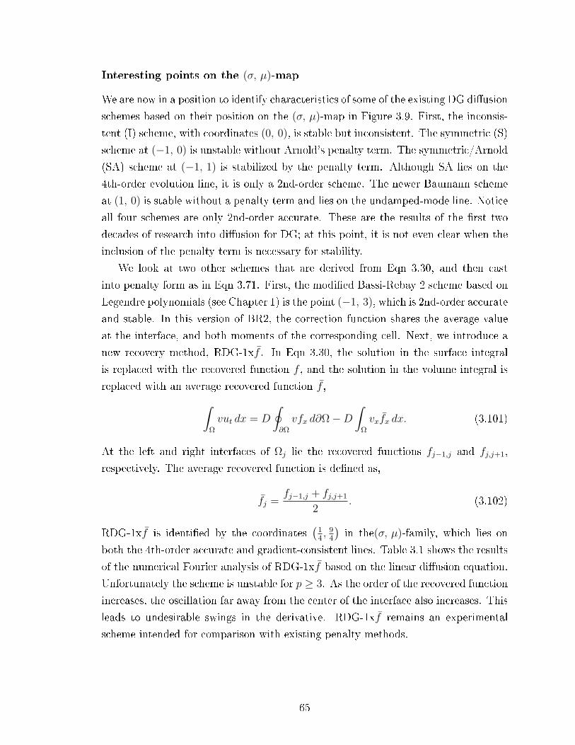
Interesting points on the (σ, µ)-map
We are now in a position to identify characteristics of some of the existing DG diusion
schemes based on their position on the (σ, µ)-map in Figure 3.9. First, the inconsis-
tent (I) scheme, with coordinates (0, 0), is stable but inconsistent. The symmetric (S)
scheme at (−1, 0) is unstable without Arnold's penalty term. The symmetric/Arnold
(SA) scheme at (−1, 1) is stabilized by the penalty term. Although SA lies on the
4th-order evolution line, it is only a 2nd-order scheme. The newer Baumann scheme
at (1, 0) is stable without a penalty term and lies on the undamped-mode line. Notice
all four schemes are only 2nd-order accurate. These are the results of the rst two
decades of research into diusion for DG; at this point, it is not even clear when the
inclusion of the penalty term is necessary for stability.
We look at two other schemes that are derived from Eqn 3.30, and then cast
into penalty form as in Eqn 3.71. First, the modied Bassi-Rebay 2 scheme based on
Legendre polynomials (see Chapter 1) is the point (−1, 3), which is 2nd-order accurate
and stable. In this version of BR2, the correction function shares the average value
at the interface, and both moments of the corresponding cell. Next, we introduce a
new recovery method, RDG-1xf . In Eqn 3.30, the solution in the surface integral
is replaced with the recovered function f , and the solution in the volume integral is
replaced with an average recovered function f ,∫Ω
vut dx = D
∮∂Ω
vfx d∂Ω−D∫
Ω
vxfx dx. (3.101)
At the left and right interfaces of Ωj lie the recovered functions fj−1,j and fj,j+1,
respectively. The average recovered function is dened as,
fj =fj−1,j + fj,j+1
2. (3.102)
RDG-1xf is identied by the coordinates(
14, 9
4
)in the(σ, µ)-family, which lies on
both the 4th-order accurate and gradient-consistent lines. Table 3.1 shows the results
of the numerical Fourier analysis of RDG-1xf based on the linear diusion equation.
Unfortunately the scheme is unstable for p ≥ 3. As the order of the recovered function
increases, the oscillation far away from the center of the interface also increases. This
leads to undesirable swings in the derivative. RDG-1xf remains an experimental
scheme intended for comparison with existing penalty methods.
65

p Min (Re (λ)) Max (Re (λ)) Max (Im (λ)) O.O.A.
1 −30.0 0.0 0.0 42 −125.2 0.0 0.0 63 −423.4 26.1 0.1 N/A4 −1280.2 404.8 0.0 N/A
Table 3.1: Numerical Fourier analysis of RDG-1xf show the scheme to be unstablefor p ≥ 3 due to positive eigenvalues. RDG-1xf is an experimental scheme.
Numerical results for various members of the (σ, µ)-family
This section introduce our famous guinea pig test case for determining the order of
accuracy of the diusion operator, and this test case is used frequently throughout
this thesis. We introduce the linear diusion equation with a source term,
ut = uxx + 4π2sin (2πx) , (3.103)
with the following boundary conditions on the domain x ∈ [0, 1],
u (0) = 1, (3.104)
u (1) = 0. (3.105)
The steady state solution is
u (x,∞) = 1− x+ sin (2πx) . (3.106)
We coupled the (σ, µ)-spatial discretization with a Runge-Kutta (RK) time-marching
scheme. Note the order of the RK scheme is irrelevant in this steady-state problem.
The maximum allowable time-step for RK schemes is determined by the Von Neumann
number D∆t∆x2 (VNN). The initial solution is the same as the exact solution. We let
the scheme march and slowly deviate from the exact solution; the resulting dierence
between the initial and nal solutions is considered the error. The complete numerical
results for all the test cases are found in Appendix B. Table 3.2 provides a summary
of the order of accuracy of each scheme and the total CPU time required for the
numerical solution to converge with convergence criterion of ε < 1e − 16 on the
320-cell grid. We dene ε in the L∞-norm,
ε = Max∣∣un+1j − unj
∣∣ . (3.107)
66

Numerical results show that only the recovery scheme on the 4th-order-evolution
line is indeed 4th-order accurate in the L2-error norm. The rest of the schemes on
the line are only 3rd-order accurate. Another exception on the 4th-order line is the
symmetric/Arnold scheme which is only 2nd-order. Other schemes lying elsewhere
are 2nd-order. The schemes(− 99
100, 101
100
)and
(−1
2, 3
2
)are on the thick-solid line on
the (σ, µ)-map, indicating the highest possible VNN number. Numerical experiment
conrms these schemes are of 3rd-order and exhibit good convergence speed. They are
able to utilize the maximum VNN of 0.20, making them among the fastest schemes
for time-accurate problems. This maximum VNN is determined by tting the largest
eigenvalue of −12 into the stability domain of a 3rd-order Runge-Kutta method. The
recovery method converges at least twice as fast in comparison to other members of the
(σ, µ)-family. We conclude that the Fourier analysis of just one eigenvalue provides
limited insight to the overall order of accuracy of a scheme. We also determine the
initial projection error by looking at the magnitude of C2 (the weighting coecient
of the bad eigenvector).
The initial projection error really comes from both the good and bad eigenvectors.
The cell average of the good eigenvector is exact due to our choice of normalization;
however, the average rst gradient contains an error. We discovered the error in the
gradient of the good eigenvector matches the error in the bad eigenvector as regards
to magnitude. Hence it suces to just show the magnitude of contribution C2 of the
bad eigenvector in Table 3.2. It turns out the gradient in the bad eigenvector of all
(σ, µ)-schemes contains an O(
1β
)error; this means the order of the projection error
is really equal to the order of C2 subtracted by one (since C2 is multiplied by the bad
gradient). The numerical experiments conrm that the order of accuracy of a scheme
is determined by the minimal of the order of λ1 and order of C2 minus one.
67

Type (σ, µ, VNN) Minimum λ1 C2 u ∆u Time
λ Order Order Rate Rate (s)RDG-1xf 1
4 ,94 , 0.08 −30.0 4 6 4 5 40.4
λ1 6th-order 19 ,
199 , 0.09 −26.6 6 4 3 3 105.9
BR2 −1, 3, 0.10 −24.0 2 4 2 3 213.0Baumann 1, 0, 0.20 −12.0 2 4 2 3 1659.2
λ1 4th-order * − 12 ,
32 , 0.19 −12.6 4 4 3 3 73.0
λ1 4th-order * − 99100 ,
101100 , 0.20 −12.0 4 4 3 3 89.9
λ1 4th-order 0, 2, 0.10 −24.0 4 4 3 3 107.5λ1 4th-order 1
6 ,136 , 0.08 −28.0 4 4 3 3 108.4
λ1 4th-order 1, 3, 0.05 −48.0 4 4 3 3 213.1Symmetric/Arnold −1, 1, 0.20 −12.0 2 N/A 2 1 106.8
µ = 1 0, 1, 0.20 −12.0 2 N/A 2 3 108.8µ = 1 1, 1, 0.10 −24.0 2 N/A 2 3 207.3µ = 1 2, 1, 0.06 −36.0 2 N/A 2 3 338.8
Gradient consistent − 37 ,
4114 , 0.09 −30.0 2 8 2 3 249.3
Gradient consistent − 12 , 3, 0.08 −30.0 2 6 2 3 253.9
Gradient consistent 1, 32 , 0.08 −30.0 2 6 2 3 250.0
Random 1, 2, 0.06 −36.0 2 4 2 3 310.2Random 0, 3, 0.06 −36.0 2 4 2 3 310.9Random 3
2 , 1, 0.08 −30.0 2 4 2 3 270.2Random −1, 2, 0.18 −13.3 2 4 2 3 125.7
Table 3.2: Stability range and order of error convergence of various schemes of the(σ, µ)-family. The maximum stable Von Neumann number (VNN) is foundnumerically to the nearest one-hundredths, and the CPU time for numeri-cal convergence is given in seconds. The * symbol indicates schemes lyingon the thick solid line of the (σ, µ)-map.
68

3.3.4 The new (σ, µ, ω)-family for p = 1
In the previous section, we tacitly showed that any DG diusion scheme can be
written in terms of jumps and averages at the interface. For the penalty method in
Eqn 3.71, the terms in the RHS only involve the jump in the solution [u], and the
average of the solution derivative < ux >. It turns out RDG-2x contains terms not
found in the traditional (σ, µ)-family; for p = 1 we see a new term involving [ux]. In
order to accommodate the new term, we introduce a new three-parameter family of
DG diusion schemes called the (σ, µ, ω)-family. We add a new term with coecient
ω to the (σ, µ)-family,∫Ωj
vut dx = −D(< ux > [v] |j+ 1
2+ < ux > [v] |j− 1
2
)−D
∫Ωj
vxux dx
+ σD(< vx > [u] |j+ 1
2+ < vx > [u] |j− 1
2
)− µD
∆x
([v][u] |j+ 1
2−[v][u] |j− 1
2
),
+ ωD∆x(
[vx] [ux] |j+ 12
+ [vx] [ux] |j− 12
). (3.108)
The update scheme in matrix form is given by,
∂
∂t
(uj
∆uj
)=
D
∆x2M (T, σ, µ, ω)
(uj
∆uj
), (3.109)
M (T, σ, µ, ω) =(µ (T 1 − 2T 0 + T−1) 1−µ
2(T 1 − T−1)
6 (σ + µ) (T 1 − T−1) (3− 12ω) (T 1 − 2T 0 + T−1)− 3 (σ + µ) (T 1 + 2T 0 + T−1)
).
The choice of (σ, µ, ω) =(−1, 9
4, 1
12
)reproduces the RDG-2x, p = 1 scheme
which is 4th-order accurate. Clearly RDG-2x is a new scheme that is very dierent
from the venerable (σ, µ)-family. One may play with the idea of exploring the whole
(σ, µ, ω)-space for interesting schemes, but it is clear from the previous section that
all but one scheme is of higher order. The beauty of RDG-2x is that it automatically
generates the correct coecients and bilinear terms for the best accuracy. In the next
section, we show RDG-2x introduces more and more bilinear terms as p increases.
69

3.3.5 Bilinear form of RDG
We have succeeded in writing the 1-D form of the RDG-2x scheme of arbitrary order
as an expansion in penalty-like terms. On a uniform grid it reads,
1
D
∫Ωj
vut dx = −(< ux > [v] |j+ 1
2+ < ux > [v] |j− 1
2
)−(< u > [vx] |j+ 1
2+ < u > [vx] |j− 1
2
)−∫
Ωj
vxux dx
+R0
∆x
([u] [v] |j+ 1
2+ [u] [v] |j− 1
2
)+R1∆x
([ux] [vx] |j+ 1
2+ [ux] [vx] |j− 1
2
)+R2∆x
([uxx] [v] |j+ 1
2+ [uxx] [v] |j− 1
2
)+R3∆x3
([uxxx] [vx] |j+ 1
2+ [uxxx] [vx] |j− 1
2
)+R4∆x3
([uxxxx] [v] |j+ 1
2+ [uxxxx] [v] |j− 1
2
)+R5∆x5
([uxxxxx] [vx] |j+ 1
2+ [uxxxxx] [vx] |j− 1
2
)+R6∆x5
([uxxxxxx] [v] |j+ 1
2+ [uxxxxxx] [v] |j− 1
2
)+ ... (3.110)
It is seen that the i-th bilinear penalty term, with coecient Ri, contains the jump
in the i-th derivative of u and the jump in either v or vx, depending on whether the
index i is even or odd, respectively. For an RDG scheme based on a polynomial space
of degree p, the index running from 0 to p, the coecients Ri are given in Table 3.3
for schemes up to p = 5.
p µ = −R0 R1 R2 R3 R4 R5
0 1
1 94
112
2 154
364
− 380
3 17532
132
− 5192
− 16720
4 945128
351536
− 5256
− 586016
5129024
5 4851512
9512
− 634096
− 136864
7369640
19461760
Table 3.3: Coecients of the penalty-like terms in 1-D RDG-2x for p ≤ 5.
70

3.4 Numerical results for the original RDG-2x
This section is intended to be a guide to implementing RDG-2x with explicit time-
marching; one can jump over the implementation details and jump directly to the
numerical results section without loss of continuity. The implementation describes
everything from the interior scheme to recovery at the domain boundary. Next, we
show numerical results for linear advection, linear diusion, and linear advection-
diusion test cases. The advection operator is the simple upwind scheme, while the
diusion operator is where RDG-2x is applied. The numerical tests are designed to
show the dierence in order of accuracy between the advection and diusion operators,
and nally show how the two work together. For the linear diusion test case, we
run both time-accurate and steady-state problems to reveal an interesting innite-
accuracy property of the RDG-2x scheme.
3.4.1 Recovery at the domain boundary
The concepts described here apply strictly to structured grids only. This section is
meant to illustrate the basic principle of enforcing the boundary-recovered function to
satisfy the given boundary conditions. Recovery at the boundary is slightly dierent
from interior recovery; however, the concept remains the same in which the boundary-
recovered function must satisfy certain moments of the solution near the boundary.
For 1-D problems the boundary-recovered function must satisfy a function value or
a derivative at the boundary. We introduce two types of boundary-recovered func-
tions: the full boundary-recovered function fF , and the compact boundary-recovered
function fC .
Full boundary-recovered function
The full boundary-recovered function covers a larger domain, which includes the
domain boundary and the rst two cells adjacent to the boundary (see left diagram
of Figure 3.10). The polynomial order of fF and interior recovered function are the
same. We enforce fF to satisfy the p + 1 moments of the rst adjacent cell, and the
p moments of the next adjacent cell. The last condition is the Dirichlet or Neumann
condition. Let Ω1 be the rst cell adjacent to the domain boundary, and Ω2 be the
71
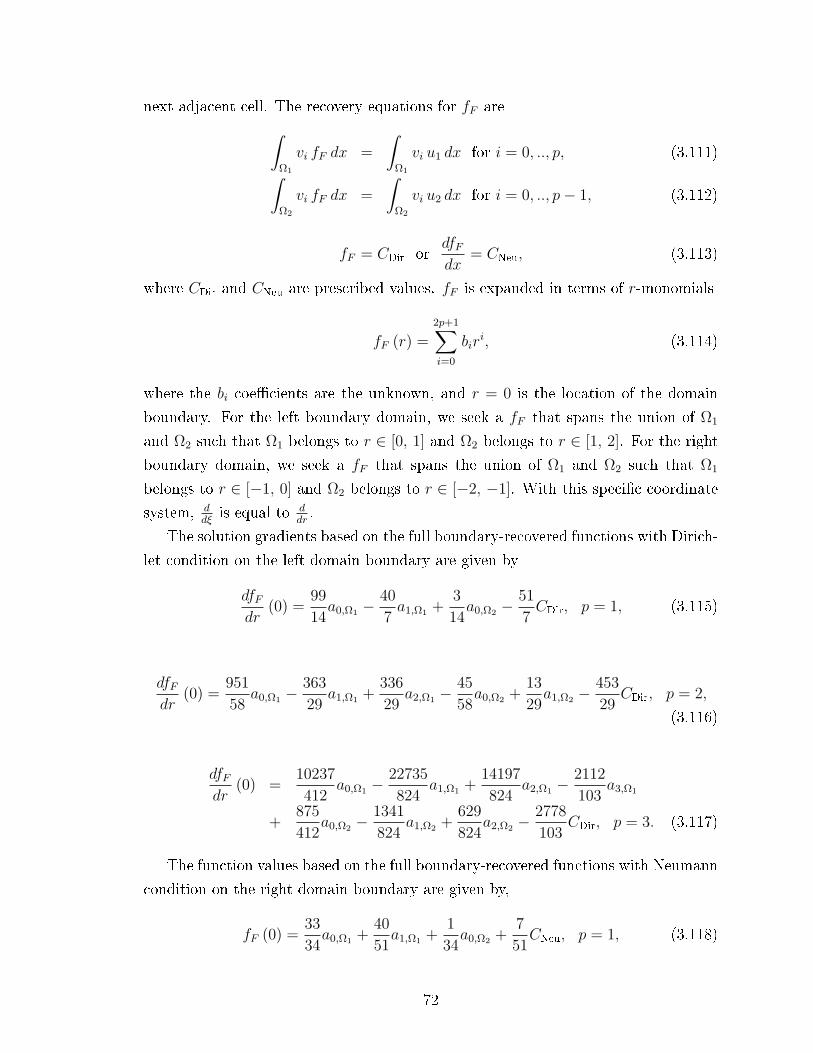
next adjacent cell. The recovery equations for fF are∫Ω1
vi fF dx =
∫Ω1
vi u1 dx for i = 0, .., p, (3.111)∫Ω2
vi fF dx =
∫Ω2
vi u2 dx for i = 0, .., p− 1, (3.112)
fF = CDir ordfFdx
= CNeu, (3.113)
where CDir and CNeu are prescribed values. fF is expanded in terms of r-monomials
fF (r) =
2p+1∑i=0
biri, (3.114)
where the bi coecients are the unknown, and r = 0 is the location of the domain
boundary. For the left boundary domain, we seek a fF that spans the union of Ω1
and Ω2 such that Ω1 belongs to r ∈ [0, 1] and Ω2 belongs to r ∈ [1, 2]. For the right
boundary domain, we seek a fF that spans the union of Ω1 and Ω2 such that Ω1
belongs to r ∈ [−1, 0] and Ω2 belongs to r ∈ [−2, −1]. With this specic coordinate
system, ddξ
is equal to ddr.
The solution gradients based on the full boundary-recovered functions with Dirich-
let condition on the left domain boundary are given by
dfFdr
(0) =99
14a0,Ω1 −
40
7a1,Ω1 +
3
14a0,Ω2 −
51
7CDir, p = 1, (3.115)
dfFdr
(0) =951
58a0,Ω1 −
363
29a1,Ω1 +
336
29a2,Ω1 −
45
58a0,Ω2 +
13
29a1,Ω2 −
453
29CDir, p = 2,
(3.116)
dfFdr
(0) =10237
412a0,Ω1 −
22735
824a1,Ω1 +
14197
824a2,Ω1 −
2112
103a3,Ω1
+875
412a0,Ω2 −
1341
824a1,Ω2 +
629
824a2,Ω2 −
2778
103CDir, p = 3. (3.117)
The function values based on the full boundary-recovered functions with Neumann
condition on the right domain boundary are given by,
fF (0) =33
34a0,Ω1 +
40
51a1,Ω1 +
1
34a0,Ω2 +
7
51CNeu, p = 1, (3.118)
72

fF (0) =317
302a0,Ω1 +
121
151a1,Ω1 +
112
151a2,Ω1 −
15
302a0,Ω2 −
13
453a1,Ω2 +
29
453CNeu, p = 2,
(3.119)
fF (0) =10237
11112a0,Ω1 +
22735
22224a1,Ω1 +
14197
22224a2,Ω1 +
352
463a3,Ω1
+875
1112a0,Ω2 +
447
7408a1,Ω2 +
629
22224a2,Ω2 +
103
2778CNeu, p = 3. (3.120)
Ω1 Ω2
u1
Ω1
u2 u1B.C.B.C.
fF fC
Figure 3.10: Stencils of full boundary-recovered function (left) and compactboundary-recovered function (right). The thick solid line indicates thedomain boundary, and B.C. stands for boundary condition, which canbe Dirichlet or Neumann.
Compact boundary-recovered function
As the name implies the compact boundary-recovered function has a smaller domain
than its cousin. fC only involves the domain boundary and the rst cell adjacent
to the boundary (see right diagram of Figure 3.10). The polynomial order of fC is
always p lower than the interior recovered function f ,
fC (r) =
p+1∑i=0
biri, (3.121)
where the bi coecients are the unknown, and r = 0 is the location of the domain
boundary. We use the same coordinate system as above. Let Ω1 be the rst cell
adjacent to the domain; the recovery equations for fC are∫Ω1
vi fF dx =
∫Ω1
vi u1 dx for i = 0, .., p, (3.122)
73

fC = CDir ordfCdx
= CNeu, (3.123)
The solution derivatives based on the compact boundary-recovered functions with
Dirichlet condition on the left domain boundary are given by
dfCdr
(0) = 6a0,Ω1 − 4a1,Ω1 − 6CDir, p = 1, (3.124)
dfCdr
(0) = 12a0,Ω1 − 10a1,Ω1 + 6a2,Ω1 − 12CDir, p = 2, (3.125)
dfCdr
(0) = 20a0,Ω1 − 18a1,Ω1 + 14a2,Ω1 − 8a3,Ω1 − 20CDir, p = 3. (3.126)
The function values based on the compact boundary-recovered functions with
Neumann condition on the right domain boundary are given by
fC (0) = a0,Ω1 +2
3a1,Ω1 +
1
6CNeu, p = 1, (3.127)
fC (0) = a0,Ω1 +5
6a1,Ω1 +
1
2a2,Ω1 +
1
12CNeu, p = 2, (3.128)
fC (0) = a0,Ω1 +9
10a1,Ω1 +
7
10a2,Ω1 +
2
5a3,Ω1 +
1
20CNeu, p = 3. (3.129)
Although we demonstrate later that the compact version is vastly inferior on a
Cartesian grid, the compact version is denitely more practical on an unstructured
grid; this is left as a future research topic.
3.4.2 Linear diusion
The numerical results for linear diusion equation is divided into three sections:
steady-state problem with periodic boundary condition, time-accurate problem with
periodic boundary condition, and steady-state problem with mixed boundary con-
ditions. The steady-state problem with periodic boundary condition is designed to
illustrate the spatial accuracy of the RDG-2x interior scheme. The time-accurate
problem with periodic boundary condition reveals the combined accuracy of RDG-
2x with Runge-Kutta time-marching. Finally, the steady-state problem with mixed
74

boundary conditions shows the results of the implementation of boundary-recovered
functions. We like to make a note that the total CPU time for each scheme is not
released because the time scale is too short for any meaningful comparison.
Steady-state problem with periodic boundary condition
We solve the linear diusion equation with a source term,
ut = uxx + 4π2sin (2πx) , (3.130)
on the domain x ∈ [0, 1]. The initial solution and nal solution are given by
u (x, t) = sin (2πx) . (3.131)
The solution is marched forward with a Runge-Kutta scheme until the change in the
solution, measured in the L∞-norm, is less than ε ≤ 1e− 15. Note that the order of
the Runge-Kutta scheme is irrelevant in a steady-state problem. Table 3.4 provides
the results for p = 1, 2 and 3. The results for p = 1 conrm the ndings from our
earlier Fourier analysis. RDG-2x (p = 1) is 4th-order accurate; however, the gradient
is 5th-order accurate! For p ≥ 2, we observe a trend in which the lower p−1 moments
are of innite accuracy. We reserve this terminology to describe solution coecients
that are solved with near computer-zero error. During our earliest investigations
we repeated the calculations with a quadruple-precision code with computer zero
of 1 × 10⁻³², and the results conrm the innite-accuracy behavior of the RDG-2x
scheme for p ≥ 2. This special property, encountered only for steady 1-D solutions
of the linear diusion equation, is explained in [43]. The order of accuracy is better
revealed in the following time-accurate test case.
Time-accurate problem with periodic boundary conditions
We solve the linear diusion equation,
ut = uxx, (3.132)
on the domain x ∈ [0, 1]. The solution for any t ≥ 0 is given by
u (x, t) = sin (2πx) e−4π2t. (3.133)
75

pNele
L2uerror
L24uerror
L24
2uerror
L24
3uerror
Rate
110
2.88×
10−
41.
35×
10−
4
201.
88×
10−
54.
37×
10−
63.
94.
940
1.19×
10−
61.
38×
10−
73.
94.
980
7.47×
10−
84.
31×
10−
93.
95.
016
04.
64×
10−
91.
34×
10−
10
4.0
5.0
320
1.70×
10−
10
3.01×
10−
12
4.7
5.4
24
9.28×
10−
10
1.13×
10−
43.
21×
10−
4
87.
32×
10−
13
9.12×
10−
75.
97×
10−
6*
6.9
5.7
165.
16×
10−
13
7.16×
10−
99.
69×
10−
8*
6.9
5.9
326.
09×
10−
13
5.60×
10−
11
1.53×
10−
9*
7.0
5.9
646.
06×
10−
15
4.37×
10−
13
2.39×
10−
11
*7.
06.
012
82.
69×
10−
15
3.43×
10−
15
3.74×
10−
13
*6.
96.
0
34
8.58×
10−
15
7.11×
10−
15
1.37×
10−
63.
17×
10−
6
82.
86×
10−
14
1.13×
10−
14
7.36×
10−
97.
42×
10−
9*
*7.
58.
712
6.51×
10−
14
1.71×
10−
14
3.05×
10−
10
2.00×
10−
10
**
7.8
8.9
164.
25×
10−
14
8.34×
10−
15
3.12×
10−
11
1.52×
10−
11
**
7.9
8.9
206.
11×
10−
15
9.83×
10−
16
5.28×
10−
12
2.06×
10−
12
**
7.9
8.9
241.
15×
10−
15
2.28×
10−
16
1.24×
10−
12
4.00×
10−
13
**
7.9
8.9
Table3.4:L
2-error
ofRDG-2xschem
eforsteady-state
problem
withperiodicboundarycondition.*standsforundetermined
order
ofaccuracy.Theextrem
elyhighaccuracy
ofthecellaverageof
thep
=2schem
e,andbothcellaverageand
rstgradientof
thep
=3schem
earereferred
toas
inniteaccuracy.
76

The nal time of the simulation is t = 0.011. The solution is marched forward in time
with a 3rd, 4th and 5th-order Runge-Kutta method (in simple notation: RK3, RK4,
and RK5) for RDG-2x schemes with p = 1, 2, and 3, respectively. The numerical
time step is determined from linear stability, or the Von Neumann number (VNN),
VNN =∆t
∆x2. (3.134)
Since ∆t scales with ∆x2, an n-th order of accuracy in time scheme will achieve 2n-
th order of accuracy in space. For example, if we naively use a 3rd-order RK with
RDG-2x (p = 2), the combined scheme only achieves the 6th-order of accuracy. A
4th-order RK must be used to unleash the full potential of RDG-2x (p = 2). The
VNN used for RK3, RK4, and RK5 are 0.15, 0.08, and 0.04, respectively. Table 3.5
provides the results for the time-accurate problem. Again, RDG-2x (p = 1) obtains
the 4th-order of accuracy; however this time around, RDG-2x (p = 2) and (p = 3)
achieve the 8th and 10th-order of accuracy, respectively. For odd p we observe that
the rst gradient is of higher order of accuracy than the cell average. Now that the
interior RDG-2x scheme is validated; we look at the boundary schemes next.
Steady-state problem with mixed boundary condition
We solve the same problem as in the σ − µ section. Consider the linear diusion
equation with a source term,
ut = uxx + 4π2sin (2πx) , (3.135)
on the domain x ∈ [0, 1]. The initial solution and nal solution are given by
u (x, t) = sin (2πx)− x+ 1. (3.136)
We enforce a Dirichlet boundary condition on the left, and a Neumann boundary
condition on the right,
u(0) = 1, (3.137)
ux (1) = 2π − 1. (3.138)
1For accurate numerical results, the nal simulation time must end exactly at t = 0.01. Even ifthe nal time is o by 1e− 8, the order of accuracy of the scheme reduces to 2nd-order.
77

pNele
L2uerror
L24uerror
L24
2uerror
L24
3uerror
Rate
110
7.32×
10−
55.
40×
10−
5
204.
96×
10−
61.
73×
10−
63.
84.
940
3.16×
10−
75.
46×
10−
83.
94.
980
1.98×
10−
81.
71×
10−
94.
05.
016
01.
24×
10−
95.
34×
10−
11
4.0
5.0
320
7.75×
10−
11
1.67×
10−
12
4.0
5.0
24
1.70×
10−
51.
18×
10−
41.
79×
10−
4
84.
05×
10−
88.
19×
10−
74.
05×
10−
68.
77.
15.
416
5.44×
10−
11
4.87×
10−
96.
57×
10−
89.
57.
35.
932
2.09×
10−
13
3.78×
10−
11
1.03×
10−
98.
07.
06.
064
1.49×
10−
14
2.94×
10−
13
1.61×
10−
11
3.8
7.0
6.0
128
5.61×
10−
14
9.87×
10−
16
2.52×
10−
13
−1.
98.
26.
0
34
2.91×
10−
81.
94×
10−
89.
68×
10−
72.
25×
10−
6
83.
30×
10−
11
1.13×
10−
11
5.04×
10−
95.
07×
10−
99.
710.7
7.5
8.7
125.
90×
10−
13
1.38×
10−
13
2.07×
10−
10
1.36×
10−
10
9.9
10.8
7.8
8.9
163.
35×
10−
14
5.89×
10−
15
2.11×
10−
11
1.03×
10−
11
9.9
10.9
7.9
8.9
203.
74×
10−
15
5.85×
10−
16
3.57×
10−
12
1.39×
10−
12
9.8
10.3
7.9
8.9
248.
10×
10−
16
1.84×
10−
16
8.34×
10−
13
2.70×
10−
13
8.3
6.3
7.9
8.9
Table3.5:L
2-error
ofRDG-2xschem
efortime-accurate
problem
withperiodicboundarycondition.
78
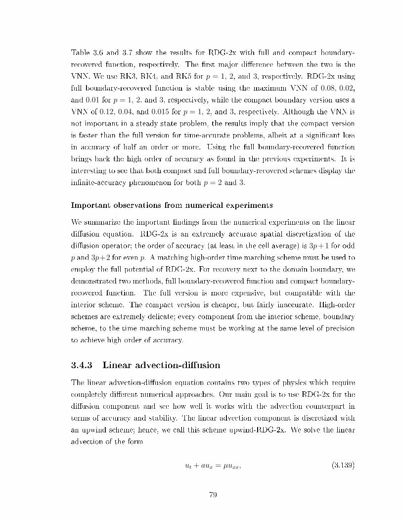
Table 3.6 and 3.7 show the results for RDG-2x with full and compact boundary-
recovered function, respectively. The rst major dierence between the two is the
VNN. We use RK3, RK4, and RK5 for p = 1, 2, and 3, respectively. RDG-2x using
full boundary-recovered function is stable using the maximum VNN of 0.08, 0.02,
and 0.01 for p = 1, 2, and 3, respectively, while the compact boundary version uses a
VNN of 0.12, 0.04, and 0.015 for p = 1, 2, and 3, respectively. Although the VNN is
not important in a steady-state problem, the results imply that the compact version
is faster than the full version for time-accurate problems, albeit at a signicant loss
in accuracy of half an order or more. Using the full boundary-recovered function
brings back the high order of accuracy as found in the previous experiments. It is
interesting to see that both compact and full boundary-recovered schemes display the
innite-accuracy phenomenon for both p = 2 and 3.
Important observations from numerical experiments
We summarize the important ndings from the numerical experiments on the linear
diusion equation. RDG-2x is an extremely accurate spatial discretization of the
diusion operator; the order of accuracy (at least in the cell average) is 3p+1 for odd
p and 3p+2 for even p. A matching high-order time marching scheme must be used to
employ the full potential of RDG-2x. For recovery next to the domain boundary, we
demonstrated two methods, full boundary-recovered function and compact boundary-
recovered function. The full version is more expensive, but compatible with the
interior scheme. The compact version is cheaper, but fairly inaccurate. High-order
schemes are extremely delicate; every component from the interior scheme, boundary
scheme, to the time-marching scheme must be working at the same level of precision
to achieve high order of accuracy.
3.4.3 Linear advection-diusion
The linear advection-diusion equation contains two types of physics which require
completely dierent numerical approaches. Our main goal is to use RDG-2x for the
diusion component and see how well it works with the advection counterpart in
terms of accuracy and stability. The linear advection component is discretized with
an upwind scheme; hence, we call this scheme upwind-RDG-2x. We solve the linear
advection of the form
ut + aux = µuxx, (3.139)
79

pNele
L2uerror
L24uerror
L24
2uerror
L24
3uerror
Rate
110
2.83×
10−
41.
67×
10−
4
201.
88×
10−
54.
93×
10−
63.
95.
040
1.19×
10−
61.
47×
10−
73.
95.
080
7.46×
10−
84.
46×
10−
94.
05.
016
04.
45×
10−
91.
37×
10−
10
4.0
5.0
320
6.42×
10−
11
2.43×
10−
12
6.1
5.8
24
9.97×
10−
10
9.09×
10−
53.
71×
10−
4
88.
82×
10−
12
7.87×
10−
76.
10×
10−
66.
96.
85.
916
7.76×
10−
12
6.65×
10−
99.
71×
10−
80.
56.
85.
932
8.22×
10−
13
5.39×
10−
11
1.53×
10−
92.
96.
95.
964
4.39×
10−
15
4.29×
10−
13
2.39×
10−
11
7.6
6.9
6.0
128
1.25×
10−
16
3.46×
10−
15
3.74×
10−
13
6.0
6.9
6.0
34
5.01×
10−
14
9.87×
10−
15
1.09×
10−
63.
93×
10−
6
81.
50×
10−
13
1.50×
10−
14
7.20×
10−
98.
45×
10−
9*
*7.
28.
812
4.87×
10−
14
9.66×
10−
15
3.03×
10−
10
2.19×
10−
10
**
7.8
9.0
164.
64×
10−
14
8.04×
10−
15
3.11×
10−
11
1.63×
10−
11
**
7.9
9.0
208.
21×
10−
15
1.53×
10−
15
5.28×
10−
12
2.18×
10−
12
**
7.9
9.0
241.
20×
10−
15
3.22×
10−
16
1.23×
10−
12
4.20×
10−
13
**
7.9
9.0
Table3.6:L
2-error
ofRDG-2xschem
eforsteady-state
problem
withmixed
boundaryconditionusingfullboundary-recovered
function.
80

pNele
L2uerror
L24uerror
L24
2uerror
L24
3uerror
Rate
110
4.62×
10−
47.
98×
10−
4
204.
17×
10−
56.
58×
10−
53.
43.
640
3.61×
10−
65.
71×
10−
63.
53.
580
3.13×
10−
75.
02×
10−
73.
53.
516
02.
73×
10−
84.
43×
10−
83.
53.
532
02.
39×
10−
93.
92×
10−
93.
53.
5
24
9.98×
10−
10
6.06×
10−
48.
88×
10−
4
89.
72×
10−
13
1.24×
10−
52.
37×
10−
5*
5.6
5.2
162.
88×
10−
13
2.67×
10−
75.
44×
10−
7*
5.5
5.4
321.
26×
10−
12
5.85×
10−
91.
21×
10−
8*
5.5
5.4
642.
63×
10−
13
1.29×
10−
10
2.67×
10−
10
*5.
55.
512
81.
53×
10−
14
2.85×
10−
12
5.88×
10−
12
*5.
55.
5
34
4.12×
10−
14
8.02×
10−
15
5.39×
10−
51.
26×
10−
4
81.
30×
10−
13
1.29×
10−
14
1.40×
10−
63.
39×
10−
6*
*5.
25.
212
2.92×
10−
13
1.93×
10−
14
1.55×
10−
73.
77×
10−
7*
*5.
45.
416
4.98×
10−
13
2.44×
10−
14
3.23×
10−
87.
83×
10−
8*
*5.
45.
420
1.44×
10−
13
1.17×
10−
14
9.50×
10−
92.
31×
10−
8*
*5.
45.
424
1.13×
10−
13
1.08×
10−
14
3.49×
10−
98.
49×
10−
9*
*5.
45.
4
Table3.7:L
2-error
ofRDG-2xschem
eforsteady-state
problem
withmixed
boundaryconditionusingcompactboundary-
recoveredfunction.
81

where a is the constant advection speed and µ is the constant diusion coecient.
The update equation is obtained by testing the equation in both space and time, after
suitable integration by parts,
∫∫vut dxdt = −a
∫∫vux dxdt+ µ
∫∫vuxx dxdt
= −a∫ (∮
vu dx−∫vxu dx
)dt
+µ
∫ (∮(vux − vxu) dx+
∫vxxu dx
)dt. (3.140)
We discretize by applying the equation to each element Ωj and replace the global
coordinate with a local coordinate,
∆x
∫Ωj
vutdξdt = −a∆t
∫ ([vu] |10 −
∫Ωj
vξu dξ
)dτ︸ ︷︷ ︸
advection
+µ∆t
∆x
∫ ([vuξ − vξu] |10 +
∫Ωj
vξξu dξ
)dτ︸ ︷︷ ︸
diusion
. (3.141)
For the advection component, the solution in the surface integral is replaced with the
upwind ux u. The upwind ux for a > 0 is given by
[vu] |10≈ v (1) uj+ 12− v (0) uj− 1
2, (3.142)
uj+ 12
= uj (ξ = 1) , (3.143)
uj− 12
= uj−1 (ξ = 1) . (3.144)
Without going through the details, the nal update matrices for p = 1 is given by,
(~uj)t =
(uj
∆uj
)t
=(
ML,p1 MC,p1 MR,p1
) ~uj−1
~uj
~uj+1
, (3.145)
ML,p1 =
[9r4
+ ν 5r4
+ ν
−15r4− 3ν −7r
4− 3ν
], (3.146)
82
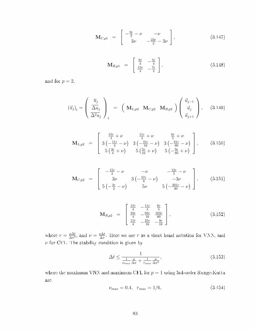
MC,p1 =
[−9r
2− ν −ν
3ν −23r2− 3ν
], (3.147)
MR,p1 =
[9r4−5r
415r4−7r
4
], (3.148)
and for p = 2,
(~uj)t =
uj
∆uj
∆2uj
t
=(
ML,p2 MC,p2 MR,p2
) ~uj−1
~uj
~uj+1
, (3.149)
ML,p2 =
15r4
+ ν 11r4
+ ν 6r5
+ ν
3(−11r
4− ν)
3(−31r
16− ν)
3(−61r
80− ν)
5(
3r4
+ ν)
5(
5r16
+ ν)
5(− 9r
80+ ν) , (3.150)
MC,p2 =
−15r2− ν −ν −12r
5− ν
3ν 3(−57r
8− ν)
−3ν
5(−3r
2− ν)
5ν 5(−201r
40− ν) , (3.151)
MR,p2 =
15r4−11r
46r5
33r4−93r
16183r80
15r4−25r
16− 9r
16
, (3.152)
where r = µ∆t∆x2 , and ν = a∆t
∆x. Here we use r as a short hand notation for VNN, and
ν for CFL. The stability condition is given by
∆t ≤ 11
νmaxa
∆x+ 1
rmax
µ∆x2
, (3.153)
where the maximum VNN and maximum CFL for p = 1 using 3rd-order Runge-Kutta
are
νmax = 0.4, rmax = 1/6, (3.154)
83

and for p = 2 using 4th-order Runge-Kutta are
νmax = 0.27, rmax = 1/10. (3.155)
These maximum values are obtained numerically via Fourier analysis of the update
matrices presented above.
Numerical results for linear advection
Before we delve into the results of the combine advection and diusion operators, we
quickly review the numerical results of the DG upwind operator. We simply obtain
the DG upwind scheme by setting µ = 0. Consider the following equation to be
solved,
ut = −aux, (3.156)
where a = 1 on the domain x ∈ [0, 1]. We use a periodic boundary condition and the
following solution,
u (x, t) = sin (2π (x− at)) . (3.157)
The nal time2 of the simulation is t = 100. The CFL numbers for p = 1 and 2 follow
from the previous section, while the CFL number for p = 3 is 0.16 with RK5. The
results are presented in Appendix B. The order of error convergence in the L2-norm is
(3, 2) for(u, ∆u
)with p = 1, (5, 4, 3) for
(u, ∆u, ∆2u
)with p = 2, and (7, 8, 5, 4)
for(u, ∆u, ∆2u, ∆3u
)with p = 3.
Numerical results for linear advection-diusion
We solve a simple time-dependent linear advection-diusion problem with the follow-
ing solution,
u (t) = e−k2µtsin k (x− at) ; x ∈ [0, 2π] . (3.158)
Observe the solution becomes zero as t → ∞. Let t = 0 and k = 1 be the initial
condition, and let t = 100 be the nal time. For a xed µ = 0.01, we varied the global
Péclet number,
PeG =al
µ, (3.159)
2The time must be large enough for the error to develop fully; this is essential to determine thecorrect order of accuracy of the scheme.
84

where l is the length of the domain. The numerical results for p = 1 and p = 2 are
given in the two info-graphics below. The numbers represent the order of accuracy
of the scheme based on cell renement measured in the horizontal direction. The
diagonal lines represent lines of constant local Péclet number,
PeL =a∆x
µ. (3.160)
The info-graphic for p = 1 (see Figure 3.11) shows that the order of accuracy scales
with the local Péclet number instead of the global Péclet number. For diusion-
dominated problems, the order of accuracy approaches 4, while for advection-dominated
problems, the order of accuracy approaches 3. A similar pattern is not observed for
p = 2 (see Figure 3.12) since the error levels on the ner grids have reached computer
zero.
0.02 0.04 0.08 0.16 0.3210
−5
100
105
∆x
Pe G
3.94444
3.94444
3.94444
3.94444
3.93.9444
3.73.83.944
3.33.53.63.83.9
2.733.23.33.4
0.82.5333
Figure 3.11: Upwind-RDG-2x (p = 1) Péclet number study. Numbers indicate theorder of accuracy in the L2-norm. The left axis indicates the valueof PeG, while the dotted lines indicate contours of constant PeL. Weobserve the order of accuracy of upwind-RDG-2x decreases in the upperright corner where the advection physics dominate, reecting the orderof accuracy of the DG upwind scheme only.
3.5 RDG schemes for variable diusion coecient
We move away from the simple constant diusion coecient to study a more complex
diusion phenomenon simulated with a variable diusion coecient. The variable
85
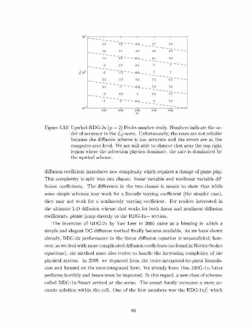
0.02 0.04 0.08 0.16 0.3210
−5
100
105
∆x
Pe G
7.880.43-7
7.78.34-6.9-2
7.67.9-0.3-13.4
6.57.57.6-7.83.5
773.8-1.2-3
776.50.7-3
5.66.16.56.61.4
4.94.94.95.15.6
4.84.74.44.24.3
Figure 3.12: Upwind-RDG-2x (p = 2) Péclet number study. Numbers indicate the or-der of accuracy in the L2-norm. Unfortunately, the rates are not reliablebecause the diusion scheme is too accurate and the errors are at thecomputer-zero level. We are still able to observe that near the top rightregion where the advection physics dominate, the rate is dominated bythe upwind scheme.
diusion coecient introduces new complexity which requires a change of game play.
This complexity is split into two classes: linear variable and nonlinear variable dif-
fusion coecients. The dierence in the two classes is meant to show that while
some simple schemes may work for a linearly varying coecient (the simpler case),
they may not work for a nonlinearly varying coecient. For readers interested in
the ultimate 1-D diusion scheme that works for both linear and nonlinear diusion
coecients, please jump directly to the RDG-1x+ section.
The invention of RDG-2x by Van Leer in 2005 came as a blessing in which a
simple and elegant DG diusion method nally became available. As we have shown
already, RDG-2x performance in the linear diusion equation is unparalleled; how-
ever, as we deal with more complicated diusion coecients (as found in Navier-Stokes
equations), the method must also evolve to handle the increasing complexity of the
physical system. In 2008, we departed from the twice-integrated-by-parts formula-
tion and focused on the once-integrated form. We already knew that RDG-1x-Naive
performs horribly and hence must be improved. In this regard, a new class of schemes
called RDG-1x-Smart arrived at the scene. The smart family recreates a more ac-
curate solution within the cell. One of the rst members was the RDG-1xf , which
86

worked well for p = 1 and 2; unfortunately, the scheme becomes unstable for p ≥ 3.
RDG-1xf suers from high-order oscillations at points far away from the center of
the Taylor expansion. As a result the interior solution derivative is completely ruined
by the oscillations. From the ashes of RDG-1xf , RDG-1x+ is born in which a new
solution enhancement technique is used to minimize oscillations within the cell.
The following section presents the schemes RDG-2x, RDG-1x-Naive, and RDG-
1xf for a general variable diusion equation. The concept of applying integration
by parts twice to the diusion operator is not commonly used by the rest of the
industry. Admittedly, integration by part twice cannot be applied if the primitive of
the diusion coecient (see Section 2.5) does not exist in terms of elementry functions
(see Section 3.5.4), or not at all (see Section 5.4) as in the system case. The variable
scalar diusion equation is given as,
ut = (µ (u)ux)x , (3.161)
where µ = µ(u) is the variable diusion coecient given as a function of the solution
u. We get the weak formulation by testing the equation with a test function v in
element Ωj, ∫Ωj
vut dt =
∫Ωj
v (µ (u)ux)x dx =
∫Ωj
v (Mx)x dx, (3.162)
where Mx = Mx (u) may or may not be an analytically integrable function of x. The
integrability of Mx dictates the number of times integration by parts can be taken.
Applying integration by parts once,∫Ωj
vut dt = [vMx]−∫
Ωj
vxMx dx, (3.163)
and ifMx is integrable (i.e.∫Mx dx = M), integration by parts one more time results
in ∫Ωj
vut dt = [vMx]− [vxM ] +
∫Ωj
vxxM dx. (3.164)
Eqn 3.163 and 3.164 are discretized by various RDG contenders. Two schemes in the
once-integrated by parts form are called
∫Ωj
vut dt =[vMx
]−∫
Ωj
vxMx dx [RDG-1x-Naive] , (3.165)∫Ωj
vut dt =[vMx
]−∫
Ωj
vxMx dx [RDG-1x-Smart] , (3.166)
87
where the surface integral terms are now replaced with the recovered function,
Mx (u) ≈ Mx (f) , (3.167)
and Mx is a special function designed to give the volume integral a better accuracy.
The juxtaposition of the terms naive and smart is meant to emphasize the im-
provement that the family of RDG-1x-Smart schemes brings. The dierence between
members of the RDG-1x-Smart family lies in the construction of Mx; currently there
are two ways to construct Mx: the aforementioned RDG-1xf and the new RDG-1x+.
RDG-1x+ uses the recovery concept for both diusion ux and solution enhancement
(see section below). As for now we briey review the RDG-1xf scheme. The special
term Mx appearing in the volume integral of RDG-1xf is dened to be the average
of the recovered functions on the left and right interfaces of Ωj,
Mx,j =1
2
(Mx (fj,j+1) + Mx (fj−1,j)
). (3.168)
Notice fj,j+1 and fj−1,j have dierent coordinate system; hence, once must be careful
when converting the recovery coordinates into the local coordinate of Ωj.
The classic twice integrated by parts scheme from the previous sections is given
by ∫Ωj
vut dt =[vMx
]−[vxM
]+
∫Ωj
vxxM dx [RDG-2x] , (3.169)
and we apply a backward integration by parts on the integral in the RHS of RDG-2x
to arrive at the RDG-3x form,∫Ωj
vut dt =[vMx
]−[vxM − vxM
]−∫
Ωj
vxMx dx [RDG-3x] . (3.170)
Notice RDG-2x and RDG-3x are mathematically equivalent; however, RDG-3x pro-
vides more creative space to deal with a non-integrable Mx that will be explained
later.
3.5.1 RDG-1x+ with recovery concept for solution enhance-
ment
Recovery was rst conceptualized for DG diusion; however, there is a much broader
application of the recovered function. Solution enhancement is the operation to in-
crease the polynomial order of a solution based on information from the surrounding
88

cells. Very often we need to enhance the polynomial order of the solution to compen-
sate for the reduction in polynomial order when a derivative of the solution is taken.
The reduction in polynomial order has a negative eect on accuracy and stability as
seen in RDG-1x-Naive. Another reason for solution enhancement is the presence of
nonlinearity in the equations.
Park at el. [29] rst experimented with solution enhancement over a large stencil
in the cell-centered RDG (cRDG) scheme. When dealing with a large multi-scale
system, the most resource-consuming part of the scheme is the implicit time-marching
algorithm. The number of equations to solve is directly proportional to the polynomial
order of the scheme; for this reason, cRDG seeks to increase the order of the scheme
without increasing the number of solution coecients. cRDG recovers a new interior
solution that satises all moments of neighboring cells. This is very similar to the
reconstruction process in a nite-volume code, except cRDG works for p ≥ 0.
The new RDG schemes make use of binary recovery for solution enhancement.
Our approach results in a smaller system of equations and eciently recycles the
recovered function: the recovered function is used for both diusion ux and solu-
tion enhancement. Consider a rough comparison of the numerical work required for
solution enhancement between RDG and cRDG on a Cartesian grid with a tensor-
product basis. cRDG solves a system of NcRDG,d (p+ 1)d equations, where NcRDG is
the number of cells in the cRDG stencil and d is the physical dimension. RDG solves
2 (p+ 1)d equations per binary recovery for NRDG,d interfaces per cell, followed by a
solution enhancement step with (p+ 1)2 + NRDG,d(p + 1) equations. Assuming n+n2
2
oating point operations (ops) to invert an (n × n) matrix via LU-decomposition,
Table 1 shows the approximate amount of computational work required for solution
enhancement by RDG and cRDG. Clearly, cRDG becomes prohibitively expensive
for higher polynomial order and physical dimension.
1-D 2-D 3-Dp RDG cRDG p RDG cRDG p RDG cRDG1 30 21 1 72 666 1 800 234362 57 45 2 231 3321 2 6291 2660853 93 78 3 528 10440 3 29392 1.49× 10⁶
4 138 120 4 1584 25425 4 100700 5.69× 10⁶
Table 3.8: Flops comparison between RDG and cRDG for solution enhancement on aCartesian grid, where (NRDG, NcRDG) is (2, 3), (5, 9), and (6, 27) for 1-D,2-D, and 3-D, respectively. RDG in 2-D and 3-D is more than an order ofmagnitude cheaper than cRDG.
89

Although the dierence in computational work required between RDG and cRDG
is signicant, cRDG's enhanced solution contains the complete set of cross-derivatives
which are useful if the PDE requires them. RDG's enhanced solution does not span
a complete higher-order polynomial space (see Figure 3.13); however, the Navier-
Stokes equations after integration by parts once no longer require the knowledge of the
cross-derivatives in the discretized solution. Ideally, the level of solution enhancement
should be optimized for the PDE being solved.
The recovery function proves to be a valuable tool; it is used for both diusion
ux and solution enhancement. Interestingly, the recovery concept represents a new
green movement in CFD, in which both subroutines and results are reused to obtain
a high order of accuracy. Starting o with the discretized solution u in each cell, a
binary recovery code is rst applied to produce all recovered functions f along the
cell interfaces. A unifying code is then applied to acquire an enhanced solution u in
each cell (see Figure 3.13). We can apply the same binary recovery code again to get
an enhanced recovery function f , and follow it up with the same solution enhance-
ment code to get a doubly enhanced solution, ˆu. Furthermore, f can be used as an
enhanced diusion ux. Solution enhancement comes at the expense of a growing
stencil in which each binary interaction brings in information from cells further away;
therefore, the optimal level of enhancement must be chosen for each PDE to ensure
the allowable time step is maximized. The process can be repeated until the desired
level of enhancement dictated by the PDE's is achieved. The following sections de-
tail two types of solution enhancement necessary for approximating the Navier-Stokes
viscous terms: the enhancement of the discretized solution and then the enhancement
of the recovered function.
u u
uu
u u
uu
^ ^
^ ^
f f f
f f f
f f
f f
f f
f = BR(u) u = SE(u,f)^
Figure 3.13: Recovery concept is used for both diusion ux and solution enhance-ment. BR stands for binary recovery; SE stands for solution enhance-ment. The cycle of BR followed by SE can be repeated over and overagain until the desired level of enhancement is achieved.
90
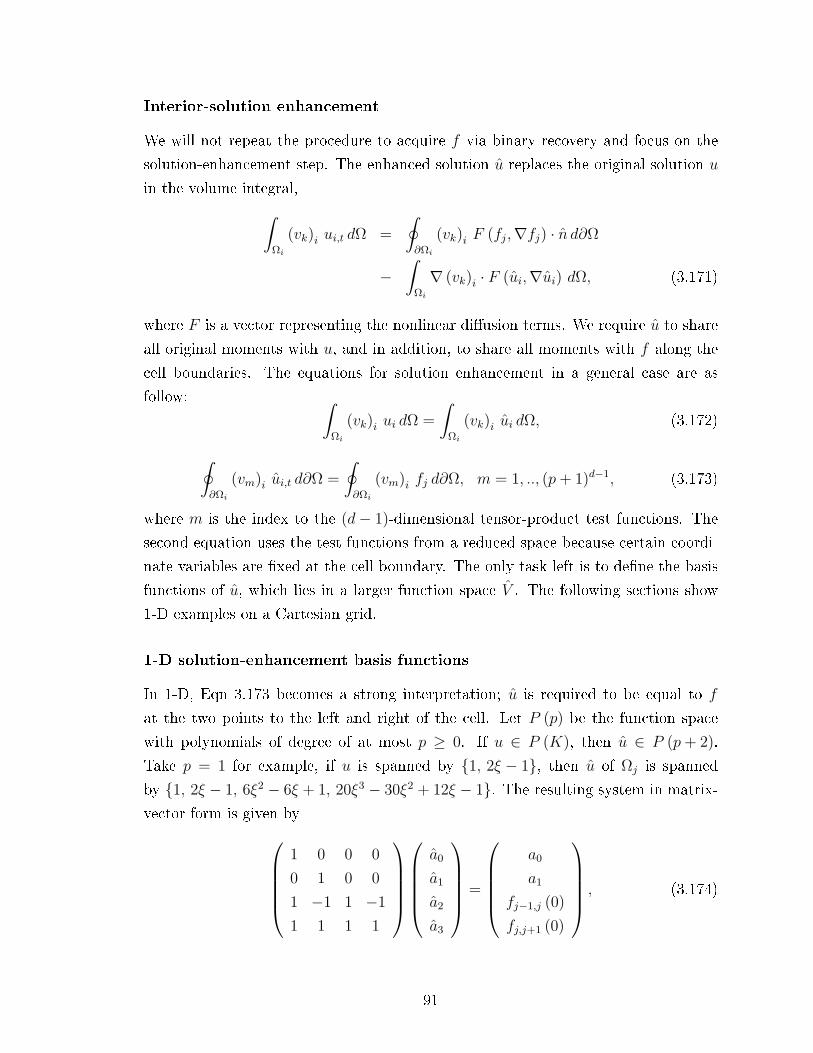
Interior-solution enhancement
We will not repeat the procedure to acquire f via binary recovery and focus on the
solution-enhancement step. The enhanced solution u replaces the original solution u
in the volume integral,∫Ωi
(vk)i ui,t dΩ =
∮∂Ωi
(vk)i F (fj,∇fj) · n d∂Ω
−∫
Ωi
∇ (vk)i · F (ui,∇ui) dΩ, (3.171)
where F is a vector representing the nonlinear diusion terms. We require u to share
all original moments with u, and in addition, to share all moments with f along the
cell boundaries. The equations for solution enhancement in a general case are as
follow: ∫Ωi
(vk)i ui dΩ =
∫Ωi
(vk)i ui dΩ, (3.172)
∮∂Ωi
(vm)i ui,t d∂Ω =
∮∂Ωi
(vm)i fj d∂Ω, m = 1, .., (p+ 1)d−1, (3.173)
where m is the index to the (d− 1)-dimensional tensor-product test functions. The
second equation uses the test functions from a reduced space because certain coordi-
nate variables are xed at the cell boundary. The only task left is to dene the basis
functions of u, which lies in a larger function space V . The following sections show
1-D examples on a Cartesian grid.
1-D solution-enhancement basis functions
In 1-D, Eqn 3.173 becomes a strong interpretation; u is required to be equal to f
at the two points to the left and right of the cell. Let P (p) be the function space
with polynomials of degree of at most p ≥ 0. If u ∈ P (K), then u ∈ P (p+ 2).
Take p = 1 for example, if u is spanned by 1, 2ξ − 1, then u of Ωj is spanned
by 1, 2ξ − 1, 6ξ2 − 6ξ + 1, 20ξ3 − 30ξ2 + 12ξ − 1. The resulting system in matrix-
vector form is given by1 0 0 0
0 1 0 0
1 −1 1 −1
1 1 1 1
a0
a1
a2
a3
=
a0
a1
fj−1,j (0)
fj,j+1 (0)
, (3.174)
91

where the top two rows come from satisfying the moments of the original solution,
and the last two rows arrive from satisfying the recovered functions on the two cell
interfaces (r = 0). Here ai are the solution coecients to u. In fact SE is so easy
with our choice of basis functions for u and u, we provide the system for p = 2 free
of charge, 1 0 0 0 0
0 1 0 0 0
0 0 1 0 0
1 −1 1 −1 1
1 1 1 1 1
a0
a1
a2
a3
a4
=
a0
a1
a2
fj−1,j (0)
fj,j+1 (0)
, (3.175)
where a4 is the solution coecient to the 4th-order Legendre polynomial. The inver-
sion of the matrix on the LHS is trivial, making solution enhancement for 1-D RDG
fast and cost ecient.
RDG-0x+
We briey introduce an experimental scheme called RDG-0x+. As the name implies,
the scheme acts upon the original weak form of the PDE's without any integration
by parts, and replaces u with a special enhanced solution, u,∫Ωi
(vk)i ui,t dΩ =
∫Ωi
(vk)i∇ · F (ui,∇ui) dΩ. (3.176)
The construction of u is similar to that of u; however, u also shares the normal
derivative, fn, of f ,
∫∂Ωi
(vm)i un,i d∂Ω =
∫∂Ωi
(vm)i fn,j d∂Ω, m = 1, .., (p+ 1)d−1. (3.177)
A comparison between RDG-1x+ and RDG-0x+ reveals many interesting dierences.
The number of terms RDG-0x+ deals with is signicantly less in 2-D and 3-D, which
translates to greater computational speed. However, this is oset by a more com-
plicated solution-enhancement procedure. Users of RDG may choose between deal-
ing with complicated terms in the 1x form, or spend more computational work to
acquire u. Currently, this experimental scheme only works with PDE without cross-
derivatives.
An interesting note: Huynh [19] analyzed various DG schemes for scalar diusion
92
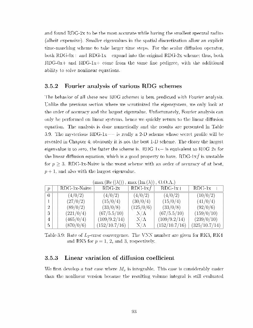
and found RDG-2x to be the most accurate while having the smallest spectral radius
(albeit expensive). Smaller eigenvalues in the spatial discretization allow an explicit
time-marching scheme to take larger time steps. For the scalar diusion operator,
both RDG-0x+ and RDG-1x+ expand into the original RDG-2x scheme; thus, both
RDG-0x+ and RDG-1x+ come from the same ne pedigree, with the additional
ability to solve nonlinear equations.
3.5.2 Fourier analysis of various RDG schemes
The behavior of all these new RDG schemes is best predicted with Fourier analysis.
Unlike the previous section where we scrutinized the eigensystem, we only look at
the order of accuracy and the largest eigenvalue. Unfortunately, Fourier analysis can
only be performed on linear systems, hence we quickly return to the linear diusion
equation. The analysis is done numerically and the results are presented in Table
3.9. The mysterious RDG-1x++ is really a 2-D scheme whose secret prole will be
revealed in Chapter 4; obviously it is not the best 1-D scheme. The closer the largest
eigenvalue is to zero, the faster the scheme is. RDG-1x+ is equivalent to RDG-2x for
the linear diusion equation, which is a good property to have. RDG-1xf is unstable
for p ≥ 3. RDG-1x-Naive is the worst scheme with an order of accuracy of at best,
p+ 1, and also with the largest eigenvalue.
(max (Re (|λ|)) , max (Im (λ)) , O.O.A.)p RDG-1x-Naive RDG-2x RDG-1xf RDG-1x+ RDG-1x++
0 (4/0/2) (4/0/2) (4/0/2) (4/0/2) (10/0/2)1 (27/0/2) (15/0/4) (30/0/4) (15/0/4) (41/0/4)2 (89/0/2) (33/0/8) (125/0/6) (33/0/8) (92/0/6)3 (221/0/4) (67/5.5/10) N/A (67/5.5/10) (159/0/10)4 (465/0/4) (109/9.2/14) N/A (109/9.2/14) (239/0/10)5 (870/0/6) (152/10.7/16) N/A (152/10.7/16) (325/10.7/14)
Table 3.9: Rate of L2-error convergence. The VNN number are given for RK3, RK4and RK5 for p = 1, 2, and 3, respectively.
3.5.3 Linear variation of diusion coecient
We rst develop a test case where Mx is integrable. This case is considerably easier
than the nonlinear version because the resulting volume integral is still evaluated
93
exactly. Consider a linear variation in µ,
µ (u) = µ0 +u
µ1
, (3.178)
where µ0,1 are constants. The integral of Mx reads,∫ (µ0ux +
uuxµ1
)dx = µ0u+
u2
2µ1
. (3.179)
We subject RDG-1x-Smart, RDG-1x-Naive and RDG-2x (RDG-3x is equivalent to
RDG-2x in this linear case) to compute the steady-state solution of the following
manufactured problem with a source term, S (x),
ut = (µ (u)ux)x + S (x) , (3.180)
S (x) = −π2cos (2πx) , (3.181)
µ (u) = u. (3.182)
Together with the initial and nal solution of
u (x) = sin (πx) , (3.183)
the diusion coecient will always be positive. We use Neumann boundary conditions
on the left and right of the physical domain x ∈ [0, 1]:
ux (0) = π, (3.184)
ux (1) = −π. (3.185)
The solution starts with the exact solution, and then marches forward in time with
a RK3, RK4, and RK5 scheme for p = 1, 2, and 3, respectively. The order of the
RK schemes is not of importance in this steady-state problem; however, high-order
RK does provide faster convergence rates. The simulation ends when the change in
solution between each time step is less than ε < 1× 10⁻¹⁵. A summary of the results
is presented in Table 3.10, while the full results is found in Appendix B. The VNN
number shows the potential dierence in speed between the schemes for time-accurate
problems. Clearly, RDG-2x and RDG-1x+ are the fastest schemes while RDG-1x-
Naive is the slowest. In terms of order of accuracy, RDG-1x-Naive lives up to its
name. RDG-1xf suers from instability for p ≥ 3 (as shown by Fourier analysis)
94

even with VNN as low as 0.0001. Although the full results in the Appendix B show
that RDG-1xf (p = 3) is potentially 10th-order for certain grids, we can no longer use
this scheme due to the lack of robustness. Our classic RDG-2x scheme performs fairly
well, but not as its former glory. RDG-2x seems to suer at the boundary (hence the
n-th and a half order results)3. Our winner for this test case is RDG-1x+ with both
the highest VNN and rate of convergence in L2-error.
Scheme p VNN Rate u Rate ∆u Rate ∆2u Rate ∆3u
1 0.07 2 3RDG-1x-Naive 2 0.02 2 3 4
3 0.01 4 5.5 4 5
1 0.15 4 5RDG-2x 2 0.08 5.5 5.5 5.5
3 0.04 7.5 7.2 7.4 7
1 0.08 4 5RDG-1xf 2 0.02 6 7 6
3 N/A N/A N/A N/A N/A
1 0.15 4 5RDG-1x+ 2 0.08 8 7 6
3 0.04 10 9 8 9
Table 3.10: Convergence rate of L2-error. The VNN number are given for RK3, RK4and RK5 for p = 1, 2, and 3, respectively.
3.5.4 Nonlinear variation of diusion coecient
The nonlinear variation in the diusion coecient will very likely generate non-
integrable diusion ux terms, especially in a system of equations. A non-integrable
diusion ux makes implementation of RDG-2x impossible. Consider the following
nonlinear diusion coecient,
µ (u) = e−u2
, (3.186)
then the diusion ux,
3An issue with the boundary scheme is usually revealed by looking at the rate of L1, L2 andL∞-error together. If the problem occurs only at the domain boundary, the rate of L1-error willbe half-an-order larger than the rate of L2-error, and the rate of L2-error will also be half-an-orderlarger than the rate of the L∞- error.
95

Mx = uxe−u2
, (3.187)
is not integrable. We briey sidetrack and talk about an attempt to implement
recovery for RDG-2x with an additional correction term in the next section.
RDG-3x
The key experimental concept within the RDG-3x scheme is to approximateMx with
a monomial which is integrable and to estimate the magnitude of the correction term.
We have demonstrated the dierence in the treatment of the volume integral between
RDG-1x-Naive and RDG-1x+ results in orders of dierence in solution accuracy. Let
us dene the dierence in the volume integrals of the two classes of RDG-1x as the
correction term. If we rewrite the RDG-2x in RDG-3x form, we observe that RDG-
1x-Naive is very similar to RDG-3x, except for the component [vxM − vxM ], which
is called the correction term,[vxM − vxM
]≈∫vx
ˆMx dx−∫vxMx dx. (3.188)
Our numerical results for RDG-1x shows the correction term changes the scheme from
2nd-order to 4th-order for p = 1, and from 2nd-order to 6th-order for p = 2, clearly
revealing the correction term is O (∆x2). With the magnitude of the correction term
in mind, we proceed to approximate localMx and recovered Mx(j,j+1) with monomials,
Mx∼= Nx = Σp
i=1aixi−1, (3.189)
Mx(j,j+1)∼= Nx(j,j+1) = Σ2p+1
i=1 bixi−1, (3.190)
where ai and bi are unknown coecients to solve for via the following projections,∫Ωj∪Ωj+1
xiMx dx =
∫Ωj∪Ωj+1
xiNx dx, (3.191)∫Ωj
xiMx dx =
∫Ωj
xiNx dx. (3.192)
The monomials are easily integrable,∫Nx dx = Σp
i=1ai
∫xi−1 dx+ c, (3.193)∫
Nx dx = Σ2p+1i=1 bi
∫xi−1 dx+ c. (3.194)
96

with unknown constants, c and c. The constants are calibrated with the knowledge
that [vxM−vxM ] ≈ O (∆x2). In order to make the correction term small, we enforced
the following in the weak sense,∫Ωj
Nx dx =
∫Ωj
Nx dx. (3.195)
Note these constants are not unique, there exist dierent constants for each interface
and element. This scheme ultimately proved to be unstable, and the complexity makes
it dicult to implement in multi-dimensional cases. This concludes our attempt to
use RDG-2x for nonlinear uxes.
Numerical results for nonlinear diusion coecient
We present the following manufactured solution for the nonlinear diusion equation,
ut =(uxe
−u2)x
+ S (x, t) , (3.196)
with a source term as a function of both space and time,
S (x) = sin (πx) e−3t−e−2tsin(πx)2(−e2t+e−2tsin(πx)2
+ π2(e2t + 1 + cos (2πx)
)).
(3.197)
The initial and nal solutions are given by
u (x, t) = sin (πx) e−t, (3.198)
on the domain x ∈ [0, 1]. We advance in time with RK3, RK4, and RK5 for p = 1, 2,
and 3, respectively, until t = 1 is reached. The numerical results for RDG-1x+ are
included in Table 3.11. We do not include RDG-1x-Naive because it is of extremely
low accuracy and RDG-1xf because it is not stable for all p. The results are very
similar to the linear-variation-diusion-coecient case. In the case of p = 3 with a
coarse grid of two cells only, the odd derivatives are zero, hence they exhibit computer-
zero error.
3.6 Chapter summary
We hope we have convinced you that RDG is a very simple diusion method for DG.
The recovered function, obtained by the binary recovery operation, is used for the dif-
97

pNele
L2uerror
L24uerror
L24
2uerror
L24
3uerror
Rate
110
1.60×
10−
52.
03×
10−
4
153.
26×
10−
67.
21×
10−
63.
94.
920
1.04×
10−
69.
72×
10−
73.
94.
930
2.08×
10−
72.
32×
10−
73.
94.
940
6.60×
10−
83.
08×
10−
83.
94.
960
1.31×
10−
87.
32×
10−
93.
94.
9
24
6.54×
10−
85.
78×
10−
61.
61×
10−
5
51.
15×
10−
81.
22×
10−
64.
61×
10−
67.
76.
95.
68
2.99×
10−
10
4.57×
10−
82.
98×
10−
77.
76.
95.
810
5.14×
10−
11
9.59×
10−
97.
95×
10−
87.
87.
05.
912
1.12×
10−
11
2.68×
10−
92.
69×
10−
87.
96.
95.
916
1.22×
10−
12
3.57×
10−
10
4.83×
10−
97.
97.
05.
9
32
8.55×
10−
87.
45×
10−
18
4.42×
10−
62.
80×
10−
17
34.
06×
10−
95.
28×
10−
94.
89×
10−
71.
80×
10−
67.
5N/A
5.4
N/A
42.
98×
10−
10
2.07×
10−
10
6.85×
10−
81.
58×
10−
79.
011.2
6.8
8.4
53.
73×
10−
11
1.88×
10−
11
1.34×
10−
82.
31×
10−
89.
310.7
7.3
8.6
83.
51×
10−
13
9.93×
10−
14
3.67×
10−
10
3.69×
10−
10
9.9
11.1
7.6
8.8
102.
72×
10−
14
1.60×
10−
14
6.40×
10−
11
5.08×
10−
11
11.4
8.1
7.8
8.8
Table3.11:L
2-error
ofRDG-1x+
schem
eforsteady-state
nonlineardiusion
problem
withperiodicboundarycondition.
98

fusion ux at the cell interface. Both Fourier analysis and numerical experiment show
the good stability and accuracy of RDG schemes. When compared to existing meth-
ods such as the (σ, µ)- family, RDG contains new bilinear terms unseen before. The
original RDG-2x is an excellent choice for linear problems. For nonlinear problems we
must extend the recovery concept to include solution enhancement. The RDG-1x+
uses enhanced solution in the volume integral to achieve high order of accuracy for
nonlinear diusion problems. We next extend these 1-D concepts to 2-D.
99

CHAPTER IV
RDG in Two-Dimensions for a Scalar
Equation
The extension of any numerical method from 1-D to multiple dimensions is not a
simple task, especially when going from 1-D to 2-D. Once the framework is nalized
from 1-D to 2-D, going to 3-D is just a matter of exercising existing concepts. One
major drawback of RDG is that the accuracy of the recovered function is dependent
on the direction; RDG only improves the accuracy in the face-normal direction, while
the accuracy in the face-parallel direction is left unchanged. This initial drawback
makes RDG-2x unsuited to deal with equations with cross-derivatives; however, this
issue is alleviated with the arrival of RDG-1x++. We rst introduce the recovery
concept, then the various variable transformations involved, and nally the concept of
solution enhancement to overcome diculty with approximating the cross-derivatives
in nonlinear diusion equations.
4.1 2-D recovery equations for binary recovery
The 2-D recovery equations for binary recovery (BR) are almost the same as the 1-D
version, with the addition of the y-coordinate. Consider the solutions in two adjacent
cells of the form presented in Eqn 2.1, where the basis functions are expressed in
terms of local coordinates (ξ, η). We look for a recovered function centered on the
100

shared interface in the form of Eqn 2.3. The 2-D recovery equations are∫∫Ωj
vjuj dxdy =
∫∫Ωj
vjfj,j+1 dxdy,∫∫Ωj+1
vj+1uj+1 dxdy =
∫∫Ωj+1
vj+1fj,j+1 dxdy. (4.1)
As we have indicated in Chapter 2, this set of equations applies to all v ∈ V , unlessstated otherwise. The face-normal direction is by default the r-coordinate, while
the face-parallel direction is the s-coordinate. Since Eqn 4.1 contains variables from
three dierent coordinate systems, we choose to express everything in terms of the
local variables for simplicity. Our rst step is to convert the integrals over the global
variables into integrals over the local variables. Secondly, we express the recovered
function in terms of local variables, i.e. f (r, s)→ f (ξ, η).
4.1.1 Transformation from global to local coordinate
Consider the mapping from an unstructured triangle T to a standard triangle TS, and
the mapping from an unstructured quadrilateral Q to a standard square QS in Figure
4.1 on the left and right, respectively. The mapping from local to global coordinates
for a triangle is,
x = (xB − xA) ξ + (xC − xA) η + xA, (4.2)
y = (yB − yA) ξ + (yC − yA) η + yA, (4.3)
and for a quadrilateral is,
x = (1− ξ) (1− η)xA + (ξ) (1− η)xB + (ξη)xC + (1− ξ) (η)xD, (4.4)
y = (1− ξ) (1− η) yA + (ξ) (1− η) yB + (ξη) yC + (1− ξ) (η) yD. (4.5)
ξ
η
1
1
0ξ
η
1
1
0A
B
C
A B
C
A
B
C
D
A B
CD
TTS
Q QS
Figure 4.1: Mapping from the global coordinates to the local coordinates. The arbi-trary triangle T is transformed into a standard triangle TS. The arbitraryquadrilateral Q is transformed into a standard square QS.
101
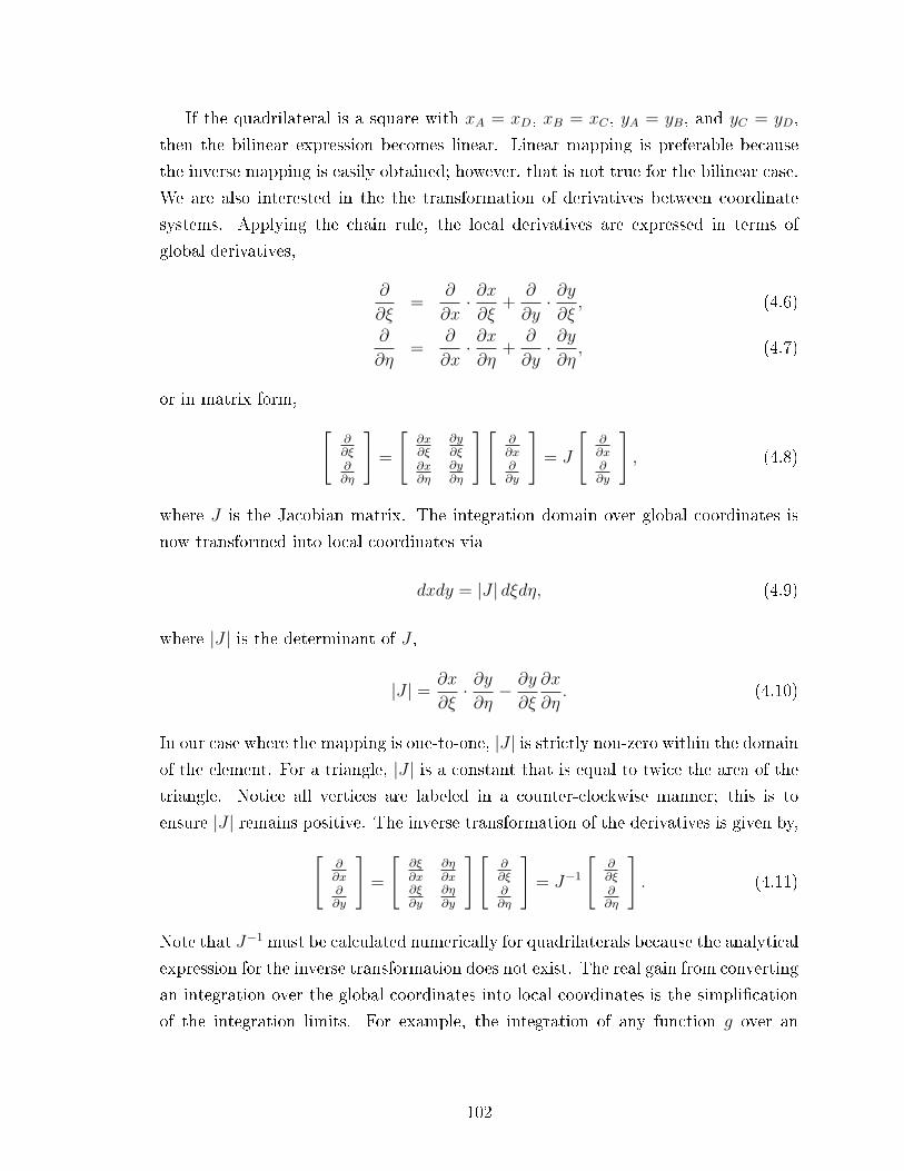
If the quadrilateral is a square with xA = xD, xB = xC , yA = yB, and yC = yD,
then the bilinear expression becomes linear. Linear mapping is preferable because
the inverse mapping is easily obtained; however, that is not true for the bilinear case.
We are also interested in the the transformation of derivatives between coordinate
systems. Applying the chain rule, the local derivatives are expressed in terms of
global derivatives,
∂
∂ξ=
∂
∂x· ∂x∂ξ
+∂
∂y· ∂y∂ξ, (4.6)
∂
∂η=
∂
∂x· ∂x∂η
+∂
∂y· ∂y∂η, (4.7)
or in matrix form, [∂∂ξ∂∂η
]=
[∂x∂ξ
∂y∂ξ
∂x∂η
∂y∂η
][∂∂x∂∂y
]= J
[∂∂x∂∂y
], (4.8)
where J is the Jacobian matrix. The integration domain over global coordinates is
now transformed into local coordinates via
dxdy = |J | dξdη, (4.9)
where |J | is the determinant of J ,
|J | = ∂x
∂ξ· ∂y∂η− ∂y
∂ξ
∂x
∂η. (4.10)
In our case where the mapping is one-to-one, |J | is strictly non-zero within the domain
of the element. For a triangle, |J | is a constant that is equal to twice the area of the
triangle. Notice all vertices are labeled in a counter-clockwise manner; this is to
ensure |J | remains positive. The inverse transformation of the derivatives is given by,[∂∂x∂∂y
]=
[∂ξ∂x
∂η∂x
∂ξ∂y
∂η∂y
][∂∂ξ∂∂η
]= J−1
[∂∂ξ∂∂η
]. (4.11)
Note that J−1 must be calculated numerically for quadrilaterals because the analytical
expression for the inverse transformation does not exist. The real gain from converting
an integration over the global coordinates into local coordinates is the simplication
of the integration limits. For example, the integration of any function g over an
102

arbitrary triangle T becomes,∫∫T
g dxdy =
∫ 1
0
∫ 1−η
0
g dξdη, (4.12)
and for an arbitrary quadrilateral Q,∫∫Q
g dxdy =
∫ 1
0
∫ 1
0
g dξdη. (4.13)
With these convenient integration limits, one can quickly apply one's favorite Gaus-
sian integration techniques. We conclude our review of nite-element coordinate
systems and look at the recovery coordinate system.
4.1.2 Tranformation from global to recovery coordinates
The recovery coordinate system, (r, s), is a bit more complicated and requires a
closer look. There are two major issues at hand, the conguration of the coordinate
system and the domain of integration. The conguration of (r, s) is based on three
simple steps: translation, rotation, scaling. We rst translate the coordinate system
to the midpoint, (xm, ym), of the interface as shown in Figure 4.2. Next, we rotate
the frame by α degrees to align the r-coordinate to the face-normal direction, and
the s-direction to the face-parallel direction. Finally, we scale the s-coordinate axis
down to unity with the r−coordinate conforming to the same scaling factor, C. The
unity-scaling provides a better condition number for solving the recovery equations.
The combined collection of linear transformations results in the following expression
in matrix form, [r
s
]= C
[cos (α) −sin (α)
sin (α) cos (α)
][x− xMy − yM
], (4.14)
where the scaling constant is determined from the length of the shared interface e,
C =2
‖e‖ . (4.15)
This mapping from (x, y) to (r, s), along with the mapping from the previous
section from (ξ, η) to (x, y), allows us to relate the three coordinate systems and
ultimately express everything in terms of the local coordinates. Our next step is to
dene the basis functions of the solution u and the recovery function f .
103
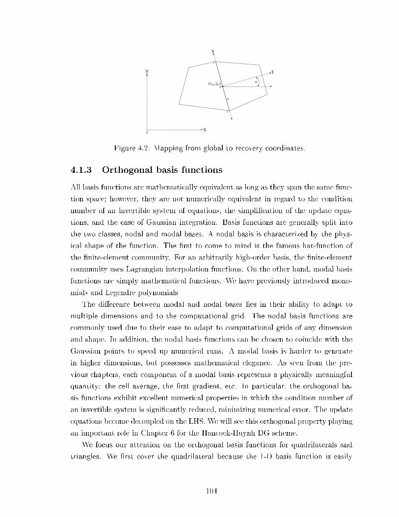
x
y
0
r
s
1
0
-1
(x m, y )m
e
α
Figure 4.2: Mapping from global to recovery coordinates.
4.1.3 Orthogonal basis functions
All basis functions are mathematically equivalent as long as they span the same func-
tion space; however, they are not numerically equivalent in regard to the condition
number of an invertible system of equations, the simplication of the update equa-
tions, and the ease of Gaussian integration. Basis functions are generally split into
the two classes, nodal and modal bases. A nodal basis is characterized by the phys-
ical shape of the function. The rst to come to mind is the famous hat-function of
the nite-element community. For an arbitrarily high-order basis, the nite-element
community uses Lagrangian interpolation functions. On the other hand, modal basis
functions are simply mathematical functions. We have previously introduced mono-
mials and Legendre polynomials
The dierence between modal and nodal bases lies in their ability to adapt to
multiple dimensions and to the computational grid. The nodal basis functions are
commonly used due to their ease to adapt to computational grids of any dimension
and shape. In addition, the nodal basis functions can be chosen to coincide with the
Gaussian points to speed up numerical runs. A modal basis is harder to generate
in higher dimensions, but possesses mathematical elegance. As seen from the pre-
vious chapters, each component of a modal basis represents a physically meaningful
quantity: the cell average, the rst gradient, etc. In particular, the orthogonal ba-
sis functions exhibit excellent numerical properties in which the condition number of
an invertible system is signicantly reduced, minimizing numerical error. The update
equations become decoupled on the LHS. We will see this orthogonal property playing
an important role in Chapter 6 for the Hancock-Huynh DG scheme.
We focus our attention on the orthogonal basis functions for quadrilaterals and
triangles. We rst cover the quadrilateral because the 1-D basis function is easily
104

extended to 2-D via tensor product. Imagine a multiplication table with the Legendre
basis functions expanded in terms of ξ on the horizontal axis, and the Legendre basis
functions expanded in terms of η on the vertical axis as shown in Table 4.1. The tensor
product automatically guarantees the resulting cross-multiplied basis functions of ξ
and η to be orthogonal on the standard square.
1 2ξ − 1 6ξ2 − 6ξ + 1 . . .
2η − 1 (2ξ − 1) (2η − 1)(6ξ2 − 6ξ + 1
)(2η − 1) . . .
6η2 − 6η + 1 (2ξ − 1)(6η2 − 6η + 1
) (6ξ2 − 6ξ + 1
) (6η2 − 6η + 1
). . .
20η3 − 30η2 + 12η − 1 (2ξ − 1)(20η3 − 30η2 + 12η − 1
) (6ξ2 − 6ξ + 1
) (20η3 − 30η2 + 12η − 1
). . .
.
.
....
.
.
.. . .
Table 4.1: Tensor-product basis for Legendre polynomials.
Unfortunately there exist no standard orthogonal basis for the standard triangle;
hence, we provide our own homebrewed method (a.k.a trial and error) for your viewing
pleasure. Based on our hard-earned experience, it is best to start with very simple
functions. Our goal is to create an orthonormal basis whose mass matrix M ,
M =
< v0, φ0 > < v0, φ1 > . . .
< v1, φ0 > < v1, φ1 >...
. . .
, (4.16)
is the identity matrix. We begin by assuming our rst basis function is of the form,
φ0 = C0,0, where C is used to indicate an unknown constant. With one equation and
one unknown constant, this equation is easily solved with φ0 =√
2. We then include
the next basis function which will contain two unknown constants. We assume a
basis function of the form, φ1 = C1,0ξ + C1,1η. The mass matrix becomes a two by
two matrix providing two conditions for the two unknown coecients. The result is
φ1 = 2√
3 (ξ − η). Our next basis function contains three unknowns, φ2 = C2,0 +
C2,1ξ + C2,2η. The pattern is to add one additional unknown constant to every
higher-order basis, together with a corresponding function in terms of ξ and η. The
methodology is not unique; we provide our sample orthogonal basis on the standard
triangle in Table 4.2.
The number of moments per cell, Nmom, is used frequently in expresssions. This
constant is dependent on the p-th order of the scheme and is dierent for standard
triangle and square. The Nmom for a standard triangle is given by
Nmom,T =(p
2+ 1)
(p+ 1) , (4.17)
105
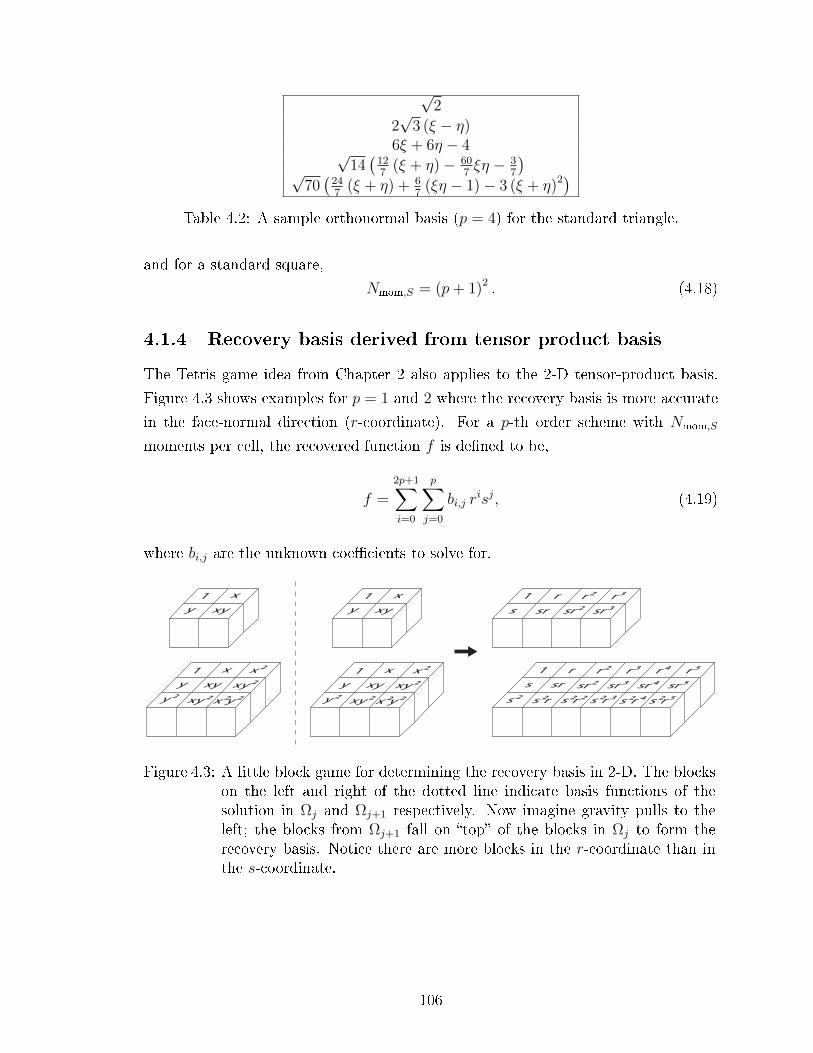
√2
2√
3 (ξ − η)6ξ + 6η − 4√
14(
127
(ξ + η)− 607ξη − 3
7
)√
70(
247
(ξ + η) + 67
(ξη − 1)− 3 (ξ + η)2)Table 4.2: A sample orthonormal basis (p = 4) for the standard triangle.
and for a standard square,
Nmom,S = (p+ 1)2 . (4.18)
4.1.4 Recovery basis derived from tensor product basis
The Tetris game idea from Chapter 2 also applies to the 2-D tensor-product basis.
Figure 4.3 shows examples for p = 1 and 2 where the recovery basis is more accurate
in the face-normal direction (r-coordinate). For a p-th order scheme with Nmom,S
moments per cell, the recovered function f is dened to be,
f =
2p+1∑i=0
p∑j=0
bi,j risj, (4.19)
where bi,j are the unknown coecients to solve for.
r2 r3r
x r
1
11
1 x2x
xyy
y2
y
r2 r3
s
s2
sr sr2 sr3
r4 r5
s2r
s srxy sr2 sr3
xy2
x2y2xy2
sr4 sr5
s2r2 s2r3 s2r4 s2r5
1 x2x
xyy
y2
xy2
x2y2xy2
x1
y xy
Figure 4.3: A little block game for determining the recovery basis in 2-D. The blockson the left and right of the dotted line indicate basis functions of thesolution in Ωj and Ωj+1 respectively. Now imagine gravity pulls to theleft; the blocks from Ωj+1 fall on top of the blocks in Ωj to form therecovery basis. Notice there are more blocks in the r-coordinate than inthe s-coordinate.
106
4.2 RDG Schemes for 2-D
This section on RDG schemes is loosely split into structured/unstructured and lin-
ear/nonlinear numerical experiments. The combination of a linear problem with an
unstructured grid allows us to focus primarily on recovery at the domain-boundary,
while the combination of a nonlinear problem with a structured grid allow us to focus
on dealing with cross-derivative terms. Common to all cases is the need to recover at
the domain boundary. Fortunately, recovery at the domain boundary is very similar
to the material presented in the previous chapter; hence, we will not go into such
detail again. For linear equations we introduce the RDG-2x, RDG-1xf , RDG-1xf ,
and RDG-1x-Naive. As for nonlinear equations, we present RDG-1x+, RDG-1x++,
and RDG-1x++CO (CO stands for Cartesian optimization).
4.2.1 Recovery at the domain boundary
Recovery at the domain boundary is a tricky business on 2-D grids; it's hard to obtain
a high-order recovered function on unstructured grids. Recall the full boundary-
recovered function, fF , requires two cells adjacent to the domain boundary. This
procedure is straightforward for structured Cartesian grid, but is complicated for
triangular grids. The compact boundary-recovered function fC , which only requires
one cell adjacent to the domain boundary, is prefered for unstructured grids.
Full boundary-recovered function for structured Cartesian grid
The full boundary-recovered function is recommended for structured Cartesian grids
due to the convenient alignment of cell centers. Figure 4.4 shows the stencil for the
full boundary-recovered function for p = 1 on the left and p = 1 on the right. Note
that we are using tensor-product basis in this example. This is very similar to the
1-D case, with the exception that the domain boundary provides p + 1 pieces of
information instead of one. Our goal is to ensure the polynomial orders of fF and the
interior recovered function are the same. We force fF to have the (p+ 1)2 moments
of the rst adjacent cell, and the (p+ 1)2− (p+ 1) moments of the next adjacent cell.
The last set of conditions come from the Dirichlet boundary condition, g (x, y), on
the domain boundary, ∂Ωe. Let Ω1 be the rst cell adjacent to the domain boundary,
107
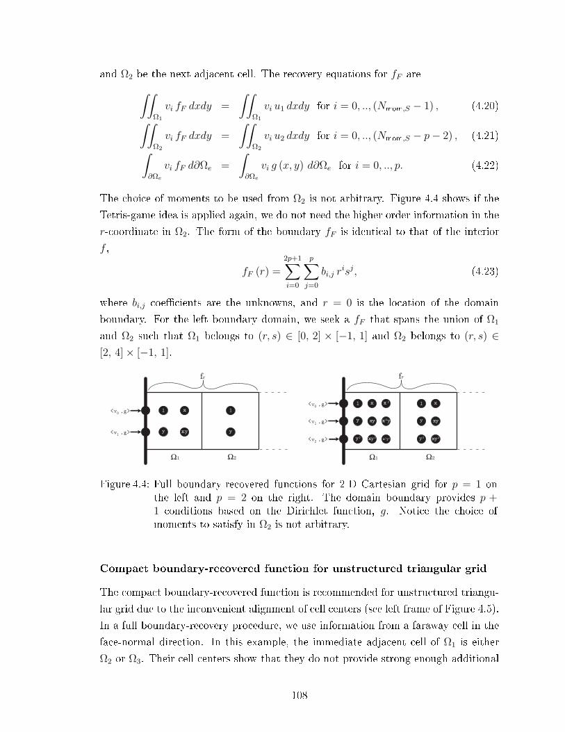
and Ω2 be the next adjacent cell. The recovery equations for fF are∫∫Ω1
vi fF dxdy =
∫∫Ω1
vi u1 dxdy for i = 0, .., (Nmom,S − 1) , (4.20)∫∫Ω2
vi fF dxdy =
∫∫Ω2
vi u2 dxdy for i = 0, .., (Nmom,S − p− 2) , (4.21)∫∂Ωe
vi fF d∂Ωe =
∫∂Ωe
vi g (x, y) d∂Ωe for i = 0, .., p. (4.22)
The choice of moments to be used from Ω2 is not arbitrary. Figure 4.4 shows if the
Tetris-game idea is applied again, we do not need the higher order information in the
r-coordinate in Ω2. The form of the boundary fF is identical to that of the interior
f ,
fF (r) =
2p+1∑i=0
p∑j=0
bi,j risj, (4.23)
where bi,j coecients are the unknowns, and r = 0 is the location of the domain
boundary. For the left boundary domain, we seek a fF that spans the union of Ω1
and Ω2 such that Ω1 belongs to (r, s) ∈ [0, 2] × [−1, 1] and Ω2 belongs to (r, s) ∈[2, 4]× [−1, 1].
Ω1 Ω2
1
Ω1 Ω2
x
y xy
1
y
1
y
y²
x
xy
xy²
x²
x²y²
x²y
1
y
y²
x
xy
xy²
<v ,g>
<v ,g>
0
1
<v ,g>
<v ,g>
0
1
<v ,g>2
fF fF
Figure 4.4: Full boundary-recovered functions for 2-D Cartesian grid for p = 1 onthe left and p = 2 on the right. The domain boundary provides p +1 conditions based on the Dirichlet function, g. Notice the choice ofmoments to satisfy in Ω2 is not arbitrary.
Compact boundary-recovered function for unstructured triangular grid
The compact boundary-recovered function is recommended for unstructured triangu-
lar grid due to the inconvenient alignment of cell centers (see left frame of Figure 4.5).
In a full boundary-recovery procedure, we use information from a faraway cell in the
face-normal direction. In this example, the immediate adjacent cell of Ω1 is either
Ω2 or Ω3. Their cell centers show that they do not provide strong enough additional
108
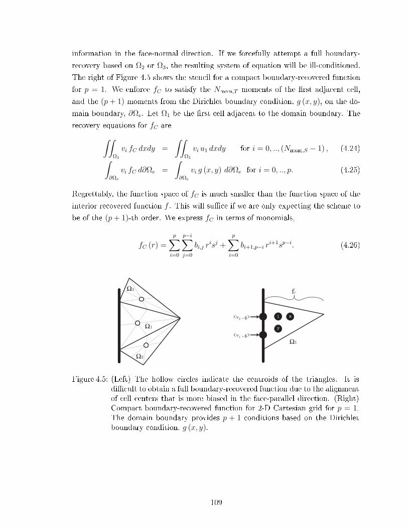
information in the face-normal direction. If we forcefully attempt a full boundary-
recovery based on Ω2 or Ω3, the resulting system of equation will be ill-conditioned.
The right of Figure 4.5 shows the stencil for a compact boundary-recovered function
for p = 1. We enforce fC to satisfy the Nmom,T moments of the rst adjacent cell,
and the (p+ 1) moments from the Dirichlet boundary condition, g (x, y), on the do-
main boundary, ∂Ωe. Let Ω1 be the rst cell adjacent to the domain boundary. The
recovery equations for fC are∫∫Ω1
vi fC dxdy =
∫∫Ω1
vi u1 dxdy for i = 0, .., (Nmom,S − 1) , (4.24)∫∂Ωe
vi fC d∂Ωe =
∫∂Ωe
vi g (x, y) d∂Ωe for i = 0, .., p. (4.25)
Regrettably, the function space of fC is much smaller than the function space of the
interior recovered function f . This will suce if we are only expecting the scheme to
be of the (p+ 1)-th order. We express fC in terms of monomials,
fC (r) =
p∑i=0
p−i∑j=0
bi,j risj +
p∑i=0
bi+1,p−i ri+1sp−i. (4.26)
Ω1
1 x
y
<v ,g>
<v ,g>
0
1
Ω1
Ω2
Ω3 fC
Figure 4.5: (Left) The hollow circles indicate the centroids of the triangles. It isdicult to obtain a full boundary-recovered function due to the alignmentof cell centers that is more biased in the face-parallel direction. (Right)Compact boundary-recovered function for 2-D Cartesian grid for p = 1.The domain boundary provides p + 1 conditions based on the Dirichletboundary condition, g (x, y).
109

4.2.2 Linear RDG schemes
We approach the linear diusion equation again as our rst test case in 2-D. This
section is divided into parts regarding structured and unstructured grids. The linear
diusion equation is given by,
ut = ∇ · ∇u = uxx + uyy. (4.27)
The weighted-residual form for Ωj is given by,∫∫Ωj
vut dt =
∫∫Ωj
v∇ · ∇u dxdy, (4.28)
The once and twice partly integrated forms are given by∫∫Ωj
vut dt =
∮∂Ωj
(v∇u) · n d∂Ω−∫∫
Ωj
∇v · ∇u dxdy, (4.29)
=
∮∂Ωj
(v∇u− u∇v) · n d∂Ω +
∫∫Ωj
u∇ · ∇v dxdy. (4.30)
RDG-2x
The rst scheme to be introduced is the original RDG-2x scheme based on twice
integrating by parts. We replace the solution in the surface integral with the recovered
function f ,∫∫Ωj
vut dt =
∮∂Ωj
(v∇f − f∇v) · n d∂Ω +
∫∫Ωj
u∇ · ∇v dxdy. (4.31)
The equation decouples nicely into x- and y-components on a Cartesian grid, resulting
in two 1-D RDG-2x schemes being applied in each direction.
RDG-1x-Naive
The underdog from the previous chapter is presented again with the sole purpose
of illustrating what not to do. RDG-1x-Naive replaces the solution in the surface
integral of the once partly integrated formulation with the recovered function,∫∫Ωj
vut dt =
∮∂Ωj
(v∇f) · n d∂Ω−∫∫
Ωj
∇v · ∇u dxdy. (4.32)
110
Since the 2-D linear diusion problem decouples nicely into two 1-D problems in the
x- and y-directions, we expect the same poor results as in one dimension.
RDG-1xf
This scheme (see previous chapter) is one of the rst members of the RDG-1x-Smart
family. RDG-1xf replaces the solution in the volume integral with the average of all
recovered functions f available in Ωj,∫∫Ωj
vut dt =
∮∂Ωj
(v∇f) · n d∂Ω−∫∫
Ωj
∇v · ∇f dxdy. (4.33)
Fourier analyses in both 1-D and in 2-D (end of this chapter) reveal the scheme is
unstable for p ≥ 3. Though the scheme had some success in 1-D, its performance
in 2-D is abysmal. The averaging of recovered functions, which mixes the accurate
information in the face-normal direction with the less accurate information in the
face-parallel direction, causes the scheme to perform poorly (on the same level as
RDG-1x-Naive). This observation leads us to our next generation scheme, RDG-1xf .
RDG-1xf
We design a scheme to take full advantage of the highly accurate information in the
face-normal direction while omitting the inaccurate face-parallel information. Our
design goal is to obtain a better ∇u for the volume integral. Since we have many
∇f candidates from each cell interface, recovery of the solution gradient involves a
least-squares procedure. Let Nj be the matrix whose rows are the vectors nj,l, where
index l cycles through the neighbors Ωl of Ωj, l = l1, . . . , lL, and let gj (~x) be the
vector of recovered normal derivatives ∂fj,l (~x) /∂nj,l, evaluated in a point ~x ∈ Ωj;
that is
Nj =
(nl1)x (nl1)y (nl1)z...
......
(nlL)x (nlL)y (nlL)z
, gj (~x) =
∂fj,l1 (~x)
∂nj,l1...
∂fj,lL (~x)
∂nj,lL
. (4.34)
The recovered gradient ∇fj (~x) then follows from
NTj Nj∇fj (~x) = NT
j gj (~x) . (4.35)
111

The resulting RDG-1xf scheme reads∫∫Ωj
vut dt =
∮∂Ωj
(v∇f) · n d∂Ω−∫∫
Ωj
∇v · ∇f dxdy. (4.36)
This system will have to be solved in all quadrature points used in evaluating the
volume integral. In 1-D the RDG-1xf scheme reduces to the RDG-1xf scheme,
meaning they share the same stability issue.
In the next section we show a series of numerical experiements to demonstrate
the performance of RDG schemes for linear problems on structured and unstructured
grids. Experiment 1 demonstrates the accuracy of the RDG-2x interior scheme. Ex-
periment 2 shows the performance of RDG schemes with the full boundary-recovered
function. Experiment 3 shows the degenerate performance of RDG schemes on un-
structured grid with the compact boundary-recovered function.
Experiment 1: Linear diusion (unsteady, periodic BC, Cartesian grid)
Our rst numerical experiment shows the performance of the interior RDG-2x scheme
on a uniform 2-D Cartesian grid. This simple problem eliminates any possible com-
plication coming from irregular grids, nonlinear diusion uxes, and boundary treat-
ment. The solution is a time-accurate decaying wave,
u (x, y, t) = sin (2πx) sin (2πy) e−t, (4.37)
where (x, y) ∈ [0, 1] × [0, 1] and the nal time is t = 0.5. The RDG-2x spatial
discretization is coupled with a Runge-Kutta temporal discretization. Figure 4.6, 4.7
and 4.8 shows the L2-error for p = 1, 2, and 3, respectively, for the cell average and
the average rst gradient. Since the problem is symmetric, the average rst gradients
in x and y directions are equal: ∆xu = ∆yu. The results are exactly the same as the
1-D case due to the nice decoupling of the diusion uxes in the x and y direction.
The rate of error convergence for RDG-2x (p = 1) is 4th-order for the cell average
and 5th-order for the average rst gradient, for RDG-2x (p = 2) is 8th-order for the
cell average and 7th-order for the rst gradient, and for RDG-2x (p = 3) is 10th-
order for the cell average and 11th-order for the rst gradient. Note the weird dip
in the error for the average rst gradient for p = 3; this is the result of averaging
the rst gradient of a sine wave on a 2-by-2 grid which results in a zero averaged
gradient. It is interesting to observe that odd-order RDG schemes have gradients
that are outperforming the cell average as found in one dimension; see Section 3.4.2.
112

0.025 0.05 0.1 0.210
−8
10−7
10−6
10−5
10−4
10−3
∆h
L2
Err
or
← Slope=5
Slope=4 →
u∆u
Figure 4.6: Experiment 1, RDG-2x (p = 1) for time-accurate problem with periodicboundary conditions. The order of error convergence is 4th-order for thecell average, and 5th-order for the averaged rst gradient.
0.025 0.05 0.1 0.2
10−13
10−12
10−11
10−10
10−9
10−8
10−7
10−6
10−5
∆h
L2
Err
or
← Slope=8
Slope=7 →
u∆u
Figure 4.7: Experiment 1, RDG-2x (p = 2) for time-accurate problem with periodicboundary conditions. The order of error convergence is 8th-order for thecell average, and 7th-order for the averaged rst gradient.
113

0.1 0.2 0.410
−14
10−13
10−12
10−11
10−10
10−9
10−8
10−7
10−6
10−5
∆h
L2
Err
or
← Slope=11
Slope=10 →
u∆u
Figure 4.8: Experiment 1, RDG-2x (p = 3) for time-accurate problem with periodicboundary conditions. The order of error convergence is 10th-order for thecell average, and 11th-order for the averaged rst gradient. The dip forthe course grid is due to the average rst gradient being zero on a 2 by 2grid.
114
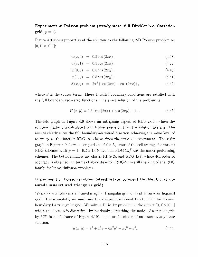
Experiment 2: Poisson problem (steady-state, full Dirchlet b.c, Cartesian
grid, p = 1)
Figure 4.9 shows properties of the solution to the following 2-D Poisson problem on
[0, 1]× [0, 1]:
u (x, 0) = 0.5 cos (2πx) , (4.38)
u (x, 1) = 0.5 cos (2πx) , (4.39)
u (0, y) = 0.5 cos (2πy) , (4.40)
u (1, y) = 0.5 cos (2πy) , (4.41)
S (x, y) = 2π2 cos (2πx) + cos (2πx) , (4.42)
where S is the source term. These Dirchlet boundary conditions are satised with
the full boundary-recovered functions. The exact solution of the problem is
U (x, y) = 0.5 cos (2πx) + cos (2πy)− 1 . (4.43)
The left graph in Figure 4.9 shows an intriguing aspect of RDG-2x in which the
solution gradient is calculated with higher precision than the solution average. The
results clearly show the full boundary-recovered function achieving the same level of
accuracy as the interior RDG-2x scheme from the previous experiment. The right
graph in Figure 4.9 shows a comparison of the L2-error of the cell average for various
RDG schemes with p = 1. RDG-1x-Naive and RDG-1xf are the under-performing
schemes. The better schemes are classic RDG-2x and RDG-1xf , where 4th-order of
accuracy is obtained. In terms of absolute error, RDG-2x is still the king of the RDG
family for linear diusion problems.
Experiment 3: Poisson problem (steady-state, compact Dirchlet b.c, struc-
tured/unstructured triangular grid)
We consider an almost structured irregular triangular grid and a structured orthogonal
grid. Unfortunately, we must use the compact recovered function at the domain
boundary for triangular grid. We solve a Dirichlet problem on the square [0, 1]× [0, 1]
where the domain is discretized by randomly perturbing the nodes of a regular grid
by 30% (see left frame of Figure 4.10). The careful choice of an exact steady state
solution,
u (x, y) = x4 + x3y − 6x2y2 − xy3 + y4, (4.44)
115
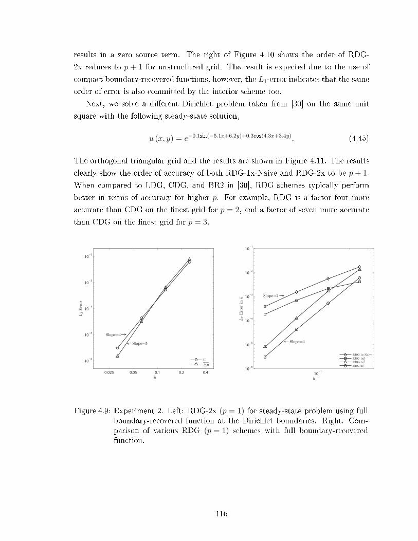
results in a zero source term. The right of Figure 4.10 shows the order of RDG-
2x reduces to p + 1 for unstructured grid. The result is expected due to the use of
compact boundary-recovered functions; however, the L1-error indicates that the same
order of error is also committed by the interior scheme too.
Next, we solve a dierent Dirichlet problem taken from [30] on the same unit
square with the following steady-state solution,
u (x, y) = e−0.1sin(−5.1x+6.2y)+0.3cos(4.3x+3.4y). (4.45)
The orthogonal triangular grid and the results are shown in Figure 4.11. The results
clearly show the order of accuracy of both RDG-1x-Naive and RDG-2x to be p + 1.
When compared to LDG, CDG, and BR2 in [30], RDG schemes typically perform
better in terms of accuracy for higher p. For example, RDG is a factor four more
accurate than CDG on the nest grid for p = 2, and a factor of seven more accurate
than CDG on the nest grid for p = 3.
0.025 0.05 0.1 0.2 0.4
10−6
10−5
10−4
10−3
10−2
h
L2Error
Slope=5
Slope=4
u
u
10−1
10−6
10−5
10−4
10−3
10−2
10−1
h
L2Errorin
u
Slope=4
Slope=2
RDG-1x-Naive
RDG-1xf
RDG-1xf
RDG-2x
-
~
Figure 4.9: Experiment 2. Left: RDG-2x (p = 1) for steady-state problem using fullboundary-recovered function at the Dirichlet boundaries. Right: Com-parison of various RDG (p = 1) schemes with full boundary-recoveredfunction.
116

0 0. 1 0. 2 0. 3 0. 4 0. 5 0. 6 0. 7 0. 8 0. 9 10
0. 1
0. 2
0. 3
0. 4
0. 5
0. 6
0. 7
0. 8
0. 9
1
x
y
10−1
10−11
10−10
10−9
10−8
10−7
10−6
10−5
10−4
10−3
10−2
∆h
L2
Err
or
p1p2p3p4
Figure 4.10: Experiment 3, RDG-2x (p = 1, 2, 3, 4) for steady-state problem usingcompact boundary-recovered function at the Dirichlet boundaries. Asample perturbed grid is shown on the left, and the graph on the rightshows the order of accuracy of the scheme to be p + 1 on the irregulartriangular grid.
0 0. 1 0. 2 0. 3 0. 4 0. 5 0. 6 0. 7 0. 8 0. 9 10
0. 1
0. 2
0. 3
0. 4
0. 5
0. 6
0. 7
0. 8
0. 9
1
x
y
10−1
10−9
10−8
10−7
10−6
10−5
10−4
10−3
10−2
∆h
L2
Err
or
p1 RDG-2xp1 RDG-1x-Naivep2 RDG-2xp2 RDG-1x-Naivep3 RDG-2xp3 RDG-1x-Naive
Figure 4.11: Experiment 3, RDG-2x and RDG-1x-Naive (p = 1, 2, 3) for steady-stateproblem using a compact boundary-recovered function at the Dirichletboundaries. It appears that RDG-2x is only slightly better than RDG-1xon a triangular grid.
117

4.2.3 Nonlinearity and cross-derivatives in RDG schemes
In addition to nonlinearity, 2-D RDG schemes require new techniques to handle cross-
derivatives properly. More precisely, the recovered function in the surface integral
needs to be more accurate in the face-parallel direction; the steps to handle the
volume integral remains the same. We present RDG-1x++ and RDG-1x++CO as
improvement over RDG-1x+. Note that RDG-1x++CO is just an optimized version
of RDG-1x++ for Cartesian grids.
RDG-1x+
We reconstruct a higher-order solution, u, to replace the interior solution in the
volume integral in the once partly integrated form of the PDE. We require u to share
all original moments with u, and, in addition, to share all moments with f along the
cell boundaries. The equations for solution enhancement in 2-D are as follows:∫Ωi
(vk)i ui dΩ =
∫Ωi
(vk)i ui dΩ, (4.46)
∮∂Ωi
(vm)i ui,t d∂Ω =
∮∂Ωi
(vm)i fj d∂Ω, m = 1, .., (p+ 1), (4.47)
In 2-D, u is required to satisfy p + 1 moments of f along a line. The choice of
basis functions for u is best illustrated by Figure 4.12. The positive x-axis repre-
sents increasing polynomial order in x, and the negative y-axis represents increasing
polynomial order in y. Consider the solid-line square to represent the original basis
functions of u. The data on the left and right boundaries of a cell add two (p + 1)-
element columns to the right of the square, while the top and bottom boundaries add
two (p+ 1)-element rows to the bottom of the square. While v and u belong to the
solution space V , u belongs to a larger solution space V such that V ⊂ V .
RDG-0x+
This experimental scheme acts upon the original weak form of the PDE's without
any integration by parts, and replaces u with a special enhanced solution, u,∫Ωi
(vk)i ui,t dΩ =
∫Ωi
(vk)i∇ · F (ui,∇ui) dΩ. (4.48)
The construction of u is similar to that of u; however, u also shares the normal
derivative, fn, of f ,
118

1 x
y
x2
y2
1 x
y xy
x2 x3
x2y x3y
y2 xy2
y3 xy3
1 x
y xy
x2 x3
x2y x3y
y2 xy2
y3 xy3
x4
y4
x4y2x3y2
x4y
xy4
x2y2
x2y3
x2y4
p = 0
p = 1
p = 2
Figure 4.12: Basis functions for u in 2-D Cartesian grid for p = 0, 1, and 2 from leftto right.
∫∂Ωi
(vm)i un,i d∂Ω =
∫∂Ωi
(vm)i fn,j d∂Ω, m = 1, .., (p+ 1). (4.49)
The main purpose of this scheme is to show that further enhancing of the solution in
the face-normal direction does not help approximating a PDE with cross-derivatives.
It is the solution in the surface integral that must be improved. In addition, the
appearance of a method not requiring integration by parts is new in nite-element
practice.
Experiment 4: nonlinear diusion without cross-derivative (time-accurate,
periodic b.c, Cartesian grid)
The following numerical experiment is designed to isolate the need for recovery-
function enhancement, and focuses on solution enhancement only. We consider the
scalar 2-D nonlinear diusion equation with a source term,
ut = e−u2
(uxx + uyy) + S (t) , (4.50)
on the domain x ∈ [0, 1], where S (t) is a time-dependent source term determined by
Mathematica software for the manufactured solution
u (x, t) = sin (2πx) sin (2πy) e−t. (4.51)
Table 4.3 shows the L2-error of the cell average at t = 1 for RDG-1x+ and RDG-
0x+. The RDG spatial discretizations are coupled with the 3rd, 4th, and 5th-order
explicit Runge-Kutta temporal schemes for p = 1, 2, and 3, respectively. RDG-0x+ is
slightly more accurate for p = 2 and 3, while both schemes obtain the same order of
119

accuracy as the original RDG-2x scheme for scalar diusion. In this problem where
the nonlinear diusion equation does not contain any cross-derivatives, both schemes
performed superbly; we next develop new techniques to handle cross-derivatives.
RDG-1x+ RDG-0x+p Cells L2-error O.O.A. p Cells L2-error O.O.A.1 18× 18 1.24e− 05 1 18× 18 1.23e− 05
24× 24 3.96e− 06 4.0 24× 24 3.96e− 06 4.030× 30 1.63e− 06 4.0 30× 30 1.63e− 06 4.036× 36 7.89e− 07 4.0 36× 36 7.91e− 07 4.0
2 18× 18 1.50e− 10 2 6× 6 5.01e− 1124× 24 1.65e− 11 7.7 12× 12 5.16e− 12 7.930× 30 2.87e− 12 7.8 18× 18 9.00e− 13 7.836× 36 6.70e− 13 8.0 24× 24 2.60e− 13 6.8
3 6× 6 8.66e− 08 3 6× 6 2.46e− 098× 8 6.35e− 09 9.1 8× 8 7.07e− 11 12.3
10× 10 7.14e− 10 9.8 10× 10 6.02e− 12 11.012× 12 1.08e− 10 10.3 12× 12 9.27e− 13 10.3
Table 4.3: Experiment 4, L2-error of the cell average for the RDG-1x+ and RDG-0x+schemes.
RDG-1x++ (Recovered-function enhancement)
Using the recovered function for the viscous uxes in 1-D problems is sucient; how-
ever, in multi-dimensional problems, the recovered function is not accurate in the
face-tangential direction of the cell boundary. The need for an accurate representa-
tion of the solution's face-tangential derivatives, such as the ones appearing in the
Navier-Stokes shear terms, is imperative for achieving overall high-order accuracy.
Our newest scheme performs binary recovery on top of the new enhanced solution u
from the previous section to obtain an enhanced recovered function f as shown in
Figure 4.13.
As mentioned before, the subroutine for recovery is the same for any level of
enhancement, with the equations for the enhanced recovered equation similiar to
those of f :
120

u u
uu
^ ^
^ ^
f f f
f f f
f f
f f
f f^ ^ ^
^ ^ ^
^ ^
^ ^
^ ^
f = BR(u)^^
Figure 4.13: The recovered function is inaccurate in the face-tangential direction. Weapply binary recovery on top of u to get an enhanced recovered functionf to improve on the accuracy of f in the face-tangential directions.
∫ΩL
(vk)L uLdΩ =
∫ΩL
(vk)L f(L,R)dΩ, ∀k s.t. vk ∈ V ,
∫ΩR
(vk)R uRdΩ =
∫ΩR
(vk)R f(L,R)dΩ, ∀k s.t. vk ∈ V . (4.52)
Here, v is a basis function of V (see Figure 4.12) and f belongs to a dierent function
space W ,
f(L,R) =∑k
bkωk, , ω ∈ W , (4.53)
where ω denotes the basis function for f (see [45] and Chapter 2 for more information
about recovery bases). In Chapter 3, we have shown the Fourier-analysis results in
Chapter 3 for the 1-D linear-diusion schemes. At the end of this chapter, we show
the 2-D Fourier-analysis results along for the other RDG schemes.
This extra layer of binary recovery comes at a hefty cost due to the increased
stencil size, which eectively decreases the maximum allowable time-step in an explicit
scheme, or increases connectivity cost in an implicit scheme. Figure 4.14 compares
the stencil size of various RDG schemes. It is worth noting that both Compact DG
(CDG) [30] and BR2 share the compact stencil of RDG-1x, but these schemes cannot
handle PDE's with cross-derivatives at the p = 0 level. Clearly, cRDG is the most
expensive of all the schemes present, while RDG-1x++CO is the optimal scheme to
handle PDE's with cross-derivatives for all p ≥ 0, if the grid is Cartesian.
121

RDG-1x RDG-1x++CO RDG-1x++ CRDG
Figure 4.14: The 2-D stencils for various RDG schemes. Stencil size has direct in-uence on the time-step of explicit time-marching schemes, and also onthe matrix density of implicit time-marching schemes.
RDG-1x++CO (Cartesian Optimization)
We draw our inspiration to optimize the RDG-1x++ scheme from dimension-splitting
techniques found in [40, 39]. We recognize the solution-enhancement step for 2-D
Cartesian grids can be factorized into 1-D steps. The convenience of such a factor-
ization is twofold. Firstly, the same operator developed for 1-D is reusable for 2-D
case; secondly, multi-dimensional codes reduce to a sequence of 1-D sweeps.
On a Cartesian grid the enhanced recovered function is too accurate in face-
normal direction; hence we eliminate the extraneous information in the face-normal
direction by using fewer moments in Eqn 4.52. Consider the stencils in Figure 4.15
used to obtain the enhanced recovered function for RDG-1x++ and RDG-1x++CO.
The thick solid line indicates the interface of interest. Since we do not need more
information in the face-normal direction, we can optimize RDG-1x++ by taking away
the two cells furthest away from the interface in the face-normal direction. This
optimization techniques require dierent sets of enhanced solutions ux and uy, which
are solution-enhanced in the x-direction and y-direction, respectively.
f of RDG-1x++CO^
f of RDG-1x++^
Figure 4.15: The stencils of the enhanced recovered function for RDG-1x++ andRDG-1x++CO on the left and right, respectively.
This section describes the steps to acquire an enhanced recovered function on a
vertical interface from uy, and because this is a factorization technique, the same steps
122

can be applied to get an enhanced recovered function on a horizontal interface from
ux. We rst cycle through all cells to get a new enhanced solution uy. Figure 4.2.3
shows a p = 1 example beginning from the left. The subscripts M , L, and R, stand
for middle, left and right, respectively. We require uyM to share all moments of uM ,
and in addition, share the moments (without the y basis) of the recovered functions
on the top and bottom faces of the cell. The resulting uyM will be enhanced in the
y-direction only, as shown in the middle of Figure 4.2.3, where the solution within the
cell now contains quadratic and cubic information in the y-direction. Our next step is
to recover the enhanced recovered function, f , from the vertically enhanced solutions
on the left and right of an interface. Using the standard binary recovery technique
with uyL and uyR as inputs, the resulting f is more accurate in both r and s directions
(see right-most frame of Figure 4.2.3). For higher p, recovery in the face-normal
direction will still be more accurate than in the face-parallel direction; nevertheless,
the slight improvement in the s-direction is sucient for high-order accuracy.
1 x
y xyuM
1 x
y xy
y xy
y xy
2 2
3 3
1 x
y xy
y xy
y xy
2 2
3 3
u L
y^ u R
y^
1 r
s rs
s rs
rs
2 2
3
r
r s
r s
r s
2
3
2
2
2
2
s3
r
r s
r s
r s
2
3
3
3
3
3
f ^
1 x
1 x
u = SE(u ) M T,M,B
y^ f = BR( , ) ^ u L
y^ u R
y^
Figure 4.16: Reduced-accuracy y-recovery, followed by standard x-recovery, to createan enhanced recovered function f for use at an interface along the y-direction.
Experiment 5: diusion-shear equation (time-accurate, periodic b.c, Carte-
sian grid)
This simple experiment adds a cross-derivative term to the linear diusion equation1,
ut = uxx + uyy + uxy. (4.54)
Despite the simplicity of this equation, RDG-2x, RDG-1x-Naive, RDG-1x+, and
RDG-0x+ completely fail to handle the cross-derivative term, resulting in an incon-
sistent (but stable) scheme. We consider the following time-accurate problem on the
unit square with periodic boundary condition and the exact solution of
1When a shear term appears, one can always nd a rotated frame in which the shear term vanishes.This theoretical insight does not help to solve the numerical problem of including inuence of cornerelements into the DG formulation.
123
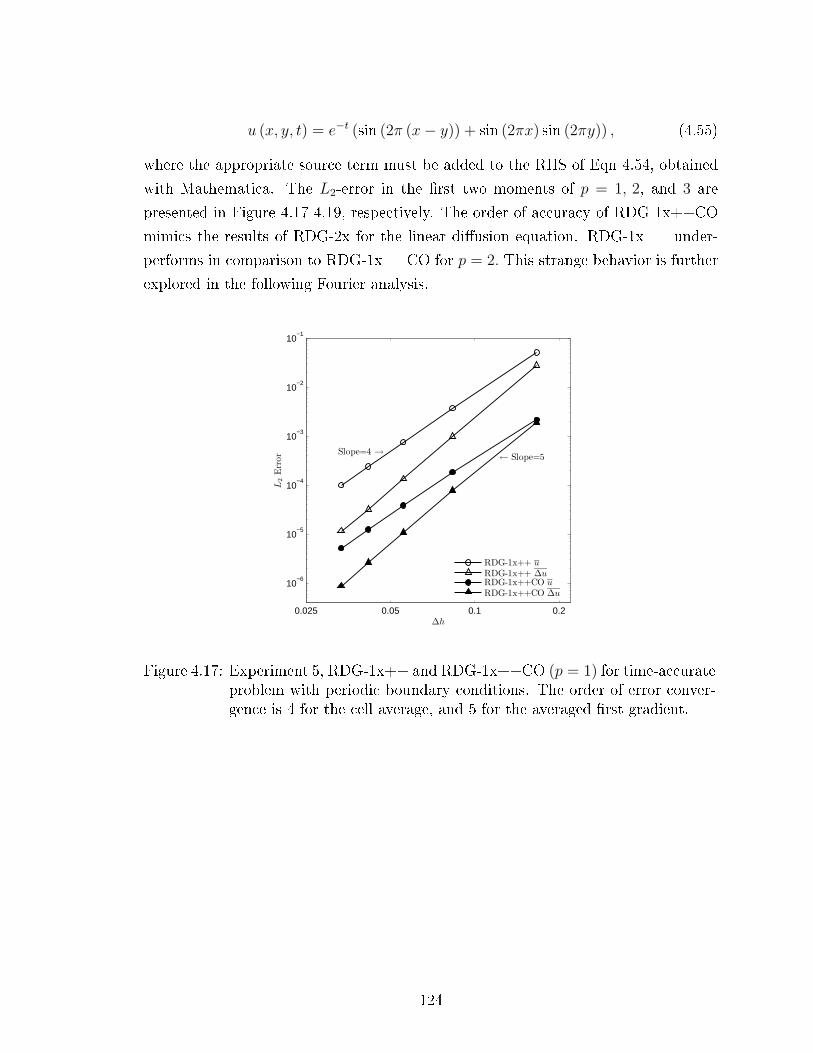
u (x, y, t) = e−t (sin (2π (x− y)) + sin (2πx) sin (2πy)) , (4.55)
where the appropriate source term must be added to the RHS of Eqn 4.54, obtained
with Mathematica. The L2-error in the rst two moments of p = 1, 2, and 3 are
presented in Figure 4.17-4.19, respectively. The order of accuracy of RDG-1x++CO
mimics the results of RDG-2x for the linear diusion equation. RDG-1x++ under-
performs in comparison to RDG-1x++CO for p = 2. This strange behavior is further
explored in the following Fourier analysis.
0.025 0.05 0.1 0.2
10−6
10−5
10−4
10−3
10−2
10−1
∆h
L2
Err
or
← Slope=5Slope=4 →
RDG-1x++ uRDG-1x++ ∆uRDG-1x++CO uRDG-1x++CO ∆u
Figure 4.17: Experiment 5, RDG-1x++ and RDG-1x++CO (p = 1) for time-accurateproblem with periodic boundary conditions. The order of error conver-gence is 4 for the cell average, and 5 for the averaged rst gradient.
124
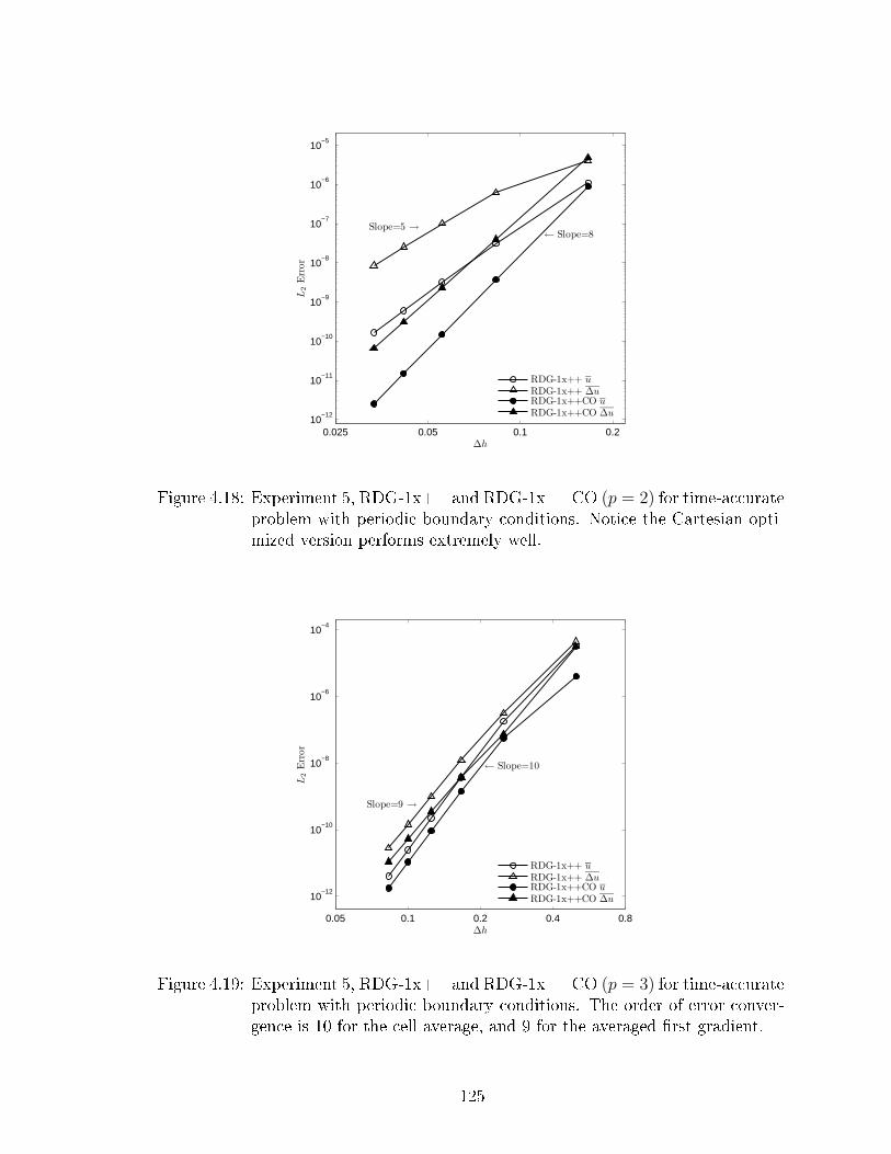
0.025 0.05 0.1 0.210
−12
10−11
10−10
10−9
10−8
10−7
10−6
10−5
∆h
L2
Err
or
← Slope=8Slope=5 →
RDG-1x++ uRDG-1x++ ∆uRDG-1x++CO uRDG-1x++CO ∆u
Figure 4.18: Experiment 5, RDG-1x++ and RDG-1x++CO (p = 2) for time-accurateproblem with periodic boundary conditions. Notice the Cartesian opti-mized version performs extremely well.
0.05 0.1 0.2 0.4 0.8
10−12
10−10
10−8
10−6
10−4
∆h
L2
Err
or
← Slope=10
Slope=9 →
RDG-1x++ uRDG-1x++ ∆uRDG-1x++CO uRDG-1x++CO ∆u
Figure 4.19: Experiment 5, RDG-1x++ and RDG-1x++CO (p = 3) for time-accurateproblem with periodic boundary conditions. The order of error conver-gence is 10 for the cell average, and 9 for the averaged rst gradient.
125
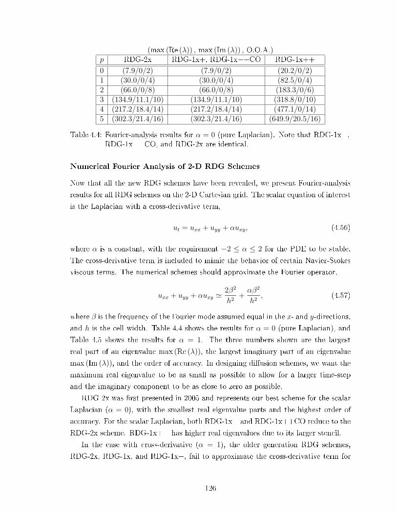
(max (Re (λ)) , max (Im (λ)) , O.O.A.)p RDG-2x RDG-1x+, RDG-1x++CO RDG-1x++
0 (7.9/0/2) (7.9/0/2) (20.2/0/2)1 (30.0/0/4) (30.0/0/4) (82.5/0/4)2 (66.0/0/8) (66.0/0/8) (183.3/0/6)3 (134.9/11.1/10) (134.9/11.1/10) (318.8/0/10)4 (217.2/18.4/14) (217.2/18.4/14) (477.1/0/14)5 (302.3/21.4/16) (302.3/21.4/16) (649.9/20.5/16)
Table 4.4: Fourier-analysis results for α = 0 (pure Laplacian). Note that RDG-1x+,RDG-1x++CO, and RDG-2x are identical.
Numerical Fourier Analysis of 2-D RDG Schemes
Now that all the new RDG schemes have been revealed, we present Fourier-analysis
results for all RDG schemes on the 2-D Cartesian grid. The scalar equation of interest
is the Laplacian with a cross-derivative term,
ut = uxx + uyy + αuxy, (4.56)
where α is a constant, with the requirement −2 ≤ α ≤ 2 for the PDE to be stable.
The cross-derivative term is included to mimic the behavior of certain Navier-Stokes
viscous terms. The numerical schemes should approximate the Fourier operator,
uxx + uyy + αuxy '2β2
h2+αβ2
h2, (4.57)
where β is the frequency of the Fourier mode assumed equal in the x- and y-directions,
and h is the cell width. Table 4.4 shows the results for α = 0 (pure Laplacian), and
Table 4.5 shows the results for α = 1. The three numbers shown are the largest
real part of an eigenvalue max (Re (λ)), the largest imaginary part of an eigenvalue
max (Im (λ)), and the order of accuracy. In designing diusion schemes, we want the
maximum real eigenvalue to be as small as possible to allow for a larger time-step
and the imaginary component to be as close to zero as possible.
RDG-2x was rst presented in 2005 and represents our best scheme for the scalar
Laplacian (α = 0), with the smallest real eigenvalue parts and the highest order of
accuracy. For the scalar Laplacian, both RDG-1x+ and RDG-1x++CO reduce to the
RDG-2x scheme. RDG-1x++ has higher real eigenvalues due to its larger stencil.
In the case with cross-derivative (α = 1), the older generation RDG schemes,
RDG-2x, RDG-1x, and RDG-1x+, fail to approximate the cross-derivative term for
126

(max (Re (λ)) , max (Im (λ)) , O.O.A.)p RDG-1x++ RDG-1x++CO
0 (20.2/0/2) (7.9/0/2)1 (82.5/0/4) (33.7/0.4/4)2 (183.6/0.76/6) (87.1/3.0/8)3 (319.2/7.59/10) (169.6/10.7/10)4 (495.3/30.43/10) (278.6/23.8/14)5 (803.6/105.5/14) (412.8/43.4/16)
Table 4.5: Fourier analysis results for α = 1 (with cross-derivative). The maximumreal eigenvalue of RDG-1x++CO is about half of that of RDG-1x++.
all p; they result in zeroth-order schemes. The only exception is for RDG-1x+ with
p = 1, which achieves 4th-order of accuracy. Of the two remaining schemes, RDG-
1x++CO allows for twice as large a time-step and obtains a higher order of accuracy
for certain p.
4.3 Chapter summary
The appearance of cross derivatives in 2-D gives rise to new numerical challenges. In
order to overcome this new problem, we present RDG-1x++ and RDG-1x++CO as
candidates. The order of accuracy achieved by these schemes is equal to or higher
than 2p + 2. In particular, the RDG-1x++CO version achieves the same order of
accuracy on a fully nonlinear problem with cross derivatives as the classic RDG-2x
on a linear diusion problem! Although the accuracy of RDG schemes is extremely
high, the true beauty of RDG, as we stress once again, is in the simplicity of concept
and implementation. Unlike other numerical methods with cookbook instructions,
we have clearly identied the obstacles stemming from a nonlinear multidimensional
problem: the nonlinear volume integral and the cross derivative in the ux integral. In
this regard, we presented solution enhancement and recovery-function enhancement
to remedy the respective issues.
We have independently studied the eect of irregular grids on RDG, and also the
performance of RDG schemes for nonlinear diusion problems. Superconvergence is
extremely dicult to achieve on an irregular grid, and currently we have yet to devise
a high-order boundary scheme for triangular grids. Our next step is to study the
performance of these new schemes on irregular grids for nonlinear diusion problems.
The 2p + 2 order of accuracy is expected to reduce to p + 1 on unstructured grids;
therefore, the future RDG schemes for unstructured grids will likely utilize a more
127

compact stencil that sacrices accuracy for eciency.
128
CHAPTER V
Navier-Stokes Equations with RDG
The original equations for viscous ow were developed more than a century ago, how-
ever, these equations are too complicated to solve even with the most advanced com-
puters today. There are actually many ow equations to decribe a viscous ow; the
three main equations are the conservation of mass, momentum and energy. The other
equations decribe physical phenomena such as chemical reactions and electromagnetic
eects. These equations go through a rigorous and scientic process of simplication
that results in the Navier-Stokes equations. The Navier-Stokes equations are only
valid for a Newtonian viscous uid in therodynamic equibrium; nevertheless, these
equations are very practical and describes a wide range of ow phenonomon. For a
detailed discussion of the Navier-Stokes equations we refer to White [46] .
5.1 1-D Navier-Stokes Equations with RDG
We present the Navier-Stokes equations in one dimension with advection component
F, and diusion component G,
Ut + F (U)x = G (U)x , (5.1)
where the conserved quantities, advection ux, and diusion ux are,
U =
ρ
ρu
ρE
, (5.2)
129
F =
ρu
p+ ρu2
ρuH
, (5.3)
G =
0
τxx
uτxx − qx
. (5.4)
The advection component simply consists of the ux terms from the Euler equations,
while the diusion component includes both the viscous stress and the heat ux. Our
numerical strategy is to apply an upwind ux to the advection component, and RDG
to the diusion component. It is easier to work with conserved variables for the sake
of conservation; however, the quantities appearing in the diusion ux are frequently
given in terms of primitive variables. For the shear stress component, τxx, we assume
a Newtonian uid and apply Stokes' hypothesis (λ = −23µ) to get an approximation,
τxx = (2µ+ λ)ux =4
3µux. (5.5)
The heat ux qx is given by Fourier's law,
qx = −κµ ∂
∂x
(p
ρ
), (5.6)
κ =γ
Pr (γ − 1), (5.7)
Pr =4γ
9γ − 5, (5.8)
where Pr is the approximate Prandtl number for a general case. Both shear-stress
and heat-ux terms are functions of the viscosity coecient µ (T ). There are many
available viscous models for Prandtl number and viscosity coecient valid for dierent
uids and temperature ranges. For example, Sutherland's law is valid for atmospheric
air with temperatures between 200K and 1000K,
µ (T ) = µ0T0 + C
T + C
(T
T0
) 32
, (5.9)
130
with the following physical constants,
γ = 1.4, (5.10)
µ0 = 1.716× 10⁻⁵[Pa · s], (5.11)
C = 110.5[K], (5.12)
T0 = 273.1[K], (5.13)
R = 287[N ·m/kg]. (5.14)
The other thermodynamic quantities of importance are given by,
p = (γ − 1)
(ρE − 1
2ρu2
), (5.15)
H = E +p
ρ, (5.16)
a = γp
ρ= γRT, (5.17)
T =1
R
p
ρ, (5.18)
where p is the pressure, H is the total enthalpy, a is the speed of sound, and T is the
temperature.
5.1.1 Discretization of 1-D Navier-Stokes viscous terms
We proceed to obtain the weak formulation of the 1-D Navier-Stokes equations by
testing Eqn 5.1 with a test function v in space, apply integration by parts once on
131

both the advection ux and the diusion ux,∫vUt dx = −
∫vFxdx+
∫vGx dx, (5.19)
∫vFx dx =
v ρu
p+ ρu2
ρuH
−
0∫vx (p+ ρu2) dx∫vx (ρuH) dx
,
∫vGx dx =
v
043µux
43µuux + κµ ∂
∂x
(pρ
)−
0∫
43vxµux dx∫ (
43vxµuux + vxκµ
(pρ
)x
)dx
.
We use the following shorthand notation for the conservative variables U0 = ρ, U1 =
ρu, U2 = ρE, and express quantities in the RHS of the weak formulation in terms of
the conservative variables,
u =U1
U0
, (5.20)
p = (γ − 1)
(U2 −
U21
2U0
), (5.21)
H =U2 + p
U0
. (5.22)
Fortunately, these are the only terms we need to express in terms of the conservative
variables since all other thermodynamic variables are related back to p and ρ. We
now discretize the weak equations on a local element Ωj with x ∈[xj− 1
2, xj+ 1
2
]; the
transformation to local coordinates in space reads,
ξ =x− xj− 1
2
∆x,∂ξ
∂x=
1
∆x≡ 1
h.
132

The goal is to transform all global derivatives into local derivatives, then the governing
equations reads,
∆x
∫Ωj
vUt dξ = −∫
Ωj
vFξdξ +
∫Ωj
vGξ dξ, (5.23)
∫Ωj
vFξ dξ =
v ρu
p+ ρu2
ρuH
ξ=1
ξ=0
−∫
Ωj
vξ
ρu
p+ ρu2
ρuH
dξ, (5.24)
∫Ωj
vGξ dξ =1
h
v
043µuξ
43µuuξ + κµ ∂
∂ξ
(pρ
)ξ=1
ξ=0
−1
h
0∫
Ωj
43vξµuξ dξ∫
Ωj
43vξµuuξ + κ (vξµ)ξ
pρdξ
, (5.25)
We may handle the computation of the F ux with an approximate Riemann solver;
here, we focus our attention on the G ux. The recovery procedure generates three
smooth functions, one for each conservative variable across the interface. However,
acquiring the exact derivatives for terms like uξ, µξ and(pρ
)ξis rather complicated,
hence a numerical approach is preferred. We refer to Appendix A for a discussion on
derivatives.
Numerical results for 1-D Navier-Stokes viscous terms
In order to bring to light the quality of RDG, this section focuses on just the diusion
terms in the Navier-Stokes equations. All of the numerical test cases are manufactured
solutions with no physical meaning, but are intended to capture the mathematical
properties of the Navier-Stokes equations and exemplify the ability of the numerical
diusion operators to solve the system.
This test case throws out the advection terms in the Navier-Stokes equation in
order to focus on the diusion terms. We keep the density variable constant since the
133

diusion ux for density is zero. Our time-accurate solution is given by,
ρ (t) = 2, (5.26)
u (t) = sin (πx) e−t, (5.27)
P (t) = 101000 + 10000 sin (πx) e−t, (5.28)
with Sutherland's law as the viscosity model with the following physical constants,
γ = 1.4, (5.29)
µ0 = 1[Pa · s], (5.30)
C = 110.5[K], (5.31)
T0 = 273.1[K], (5.32)
R = 287[N ·m/kg]. (5.33)
Notice these constants are the same as those for atmospheric air with the exception
of µ0. The real value of µ0 is too low; a higher value guarantees a larger change in
the solution in a shorter amount of time. We solve the following system, ρ
ρu
ρE
t
=
0
43µux
43µuux + κµ ∂
∂x
(pρ
)+
0
S1 (t)
S2 (t)
, (5.34)
where S1 and S2 are source terms determined by inserting the time-accurate solution
into the system of equations above, using Mathematica. In order the ascertain the
quality of the manufactured solution, we numerically compared the values of the
ux terms with the values of the source terms to ensure the source terms are not
dominating the RHS. The conserved variables are recovered across the interface and
then used to determine the nonlinear ux at the interface. The solution is marched
forward in time using a 3rd-order Runge-Kutta scheme until t = 3. The numerical
results for RDG-1x-Naive, RDG-1xf , and RDG-1x+ for p = 1 and p = 2 are presented
in Table 5.1 and 5.2. Note that only the L2 error of the total-energy variable is shown;
134
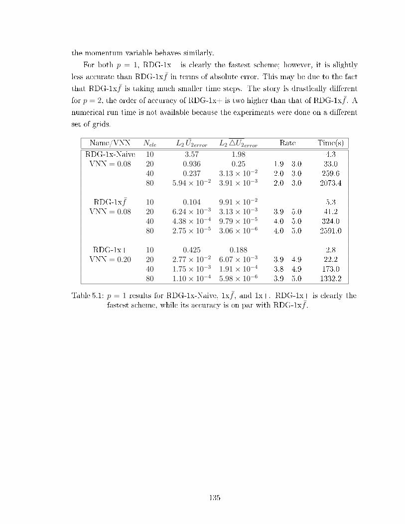
the momentum variable behaves similarly.
For both p = 1, RDG-1x+ is clearly the fastest scheme; however, it is slightly
less accurate than RDG-1xf in terms of absolute error. This may be due to the fact
that RDG-1xf is taking much smaller time steps. The story is drastically dierent
for p = 2, the order of accuracy of RDG-1x+ is two higher than that of RDG-1xf . A
numerical run time is not available because the experiments were done on a dierent
set of grids.
Name/VNN Nele L2 U2error L24U2error Rate Time(s)
RDG-1x-Naive 10 3.57 1.98 4.3VNN = 0.08 20 0.936 0.25 1.9 3.0 33.0
40 0.237 3.13× 10⁻² 2.0 3.0 259.680 5.94× 10⁻² 3.91× 10⁻³ 2.0 3.0 2073.4
RDG-1xf 10 0.104 9.91× 10⁻² 5.3VNN = 0.08 20 6.24× 10⁻³ 3.13× 10⁻³ 3.9 5.0 41.2
40 4.38× 10⁻⁴ 9.79× 10⁻⁵ 4.0 5.0 324.080 2.75× 10⁻⁵ 3.06× 10⁻⁶ 4.0 5.0 2591.0
RDG-1x+ 10 0.425 0.188 2.8VNN = 0.20 20 2.77× 10⁻² 6.07× 10⁻³ 3.9 4.9 22.2
40 1.75× 10⁻³ 1.91× 10⁻⁴ 3.8 4.9 173.080 1.10× 10⁻⁴ 5.98× 10⁻⁶ 3.9 5.0 1332.2
Table 5.1: p = 1 results for RDG-1x-Naive, 1xf , and 1x+. RDG-1x+ is clearly thefastest scheme, while its accuracy is on par with RDG-1xf .
135
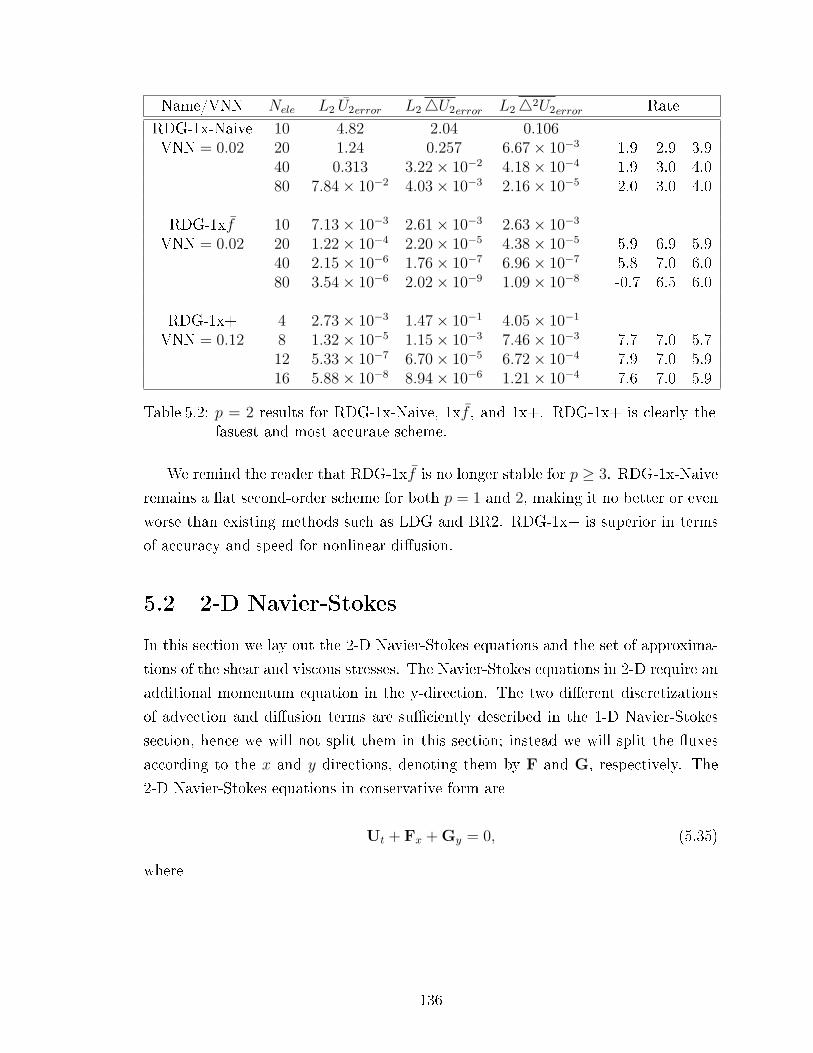
Name/VNN Nele L2 U2error L24U2error L242U2error Rate
RDG-1x-Naive 10 4.82 2.04 0.106VNN = 0.02 20 1.24 0.257 6.67× 10⁻³ 1.9 2.9 3.9
40 0.313 3.22× 10⁻² 4.18× 10⁻⁴ 1.9 3.0 4.080 7.84× 10⁻² 4.03× 10⁻³ 2.16× 10⁻⁵ 2.0 3.0 4.0
RDG-1xf 10 7.13× 10⁻³ 2.61× 10⁻³ 2.63× 10⁻³
VNN = 0.02 20 1.22× 10⁻⁴ 2.20× 10⁻⁵ 4.38× 10⁻⁵ 5.9 6.9 5.940 2.15× 10⁻⁶ 1.76× 10⁻⁷ 6.96× 10⁻⁷ 5.8 7.0 6.080 3.54× 10⁻⁶ 2.02× 10⁻⁹ 1.09× 10⁻⁸ -0.7 6.5 6.0
RDG-1x+ 4 2.73× 10⁻³ 1.47× 10⁻¹ 4.05× 10⁻¹
VNN = 0.12 8 1.32× 10⁻⁵ 1.15× 10⁻³ 7.46× 10⁻³ 7.7 7.0 5.712 5.33× 10⁻⁷ 6.70× 10⁻⁵ 6.72× 10⁻⁴ 7.9 7.0 5.916 5.88× 10⁻⁸ 8.94× 10⁻⁶ 1.21× 10⁻⁴ 7.6 7.0 5.9
Table 5.2: p = 2 results for RDG-1x-Naive, 1xf , and 1x+. RDG-1x+ is clearly thefastest and most accurate scheme.
We remind the reader that RDG-1xf is no longer stable for p ≥ 3. RDG-1x-Naive
remains a at second-order scheme for both p = 1 and 2, making it no better or even
worse than existing methods such as LDG and BR2. RDG-1x+ is superior in terms
of accuracy and speed for nonlinear diusion.
5.2 2-D Navier-Stokes
In this section we lay out the 2-D Navier-Stokes equations and the set of approxima-
tions of the shear and viscous stresses. The Navier-Stokes equations in 2-D require an
additional momentum equation in the y-direction. The two dierent discretizations
of advection and diusion terms are suciently described in the 1-D Navier-Stokes
section, hence we will not split them in this section; instead we will split the uxes
according to the x and y directions, denoting them by F and G, respectively. The
2-D Navier-Stokes equations in conservative form are
Ut + Fx + Gy = 0, (5.35)
where
136

U =
ρ
ρu
ρv
ρE
, (5.36)
F =
ρu
ρu2 + p− τxxρuv − τxy
ρuH − uτxx − vτxy + qx
, (5.37)
G =
ρv
ρuv − τyxρv2 + p− τyy
ρuvH − uτyx − vτyy + qy
. (5.38)
The viscous stresses in 2-D for a Newtonian uid are given by,
τxx = 2µ∂u
∂x+ λ
(∂u
∂x+∂v
∂y
), (5.39)
τxy = τyx = µ
(∂u
∂y+∂v
∂x
), (5.40)
τyy = 2µ∂v
∂y+ λ
(∂u
∂x+∂v
∂y
). (5.41)
Applying Stokes's hypothesis (λ = −23µ), the viscous stresses simplify to
τxx =2
3µ
(2∂u
∂x− ∂v
∂y
), (5.42)
τyy =2
3µ
(2∂v
∂y− ∂u
∂x
). (5.43)
The heat uxes are given by
qx = − γµ
Pr (γ − 1)
∂
∂x
(p
ρ
), (5.44)
qy = − γµ
Pr (γ − 1)
∂
∂y
(p
ρ
). (5.45)
The viscousity coecient µ is determined from Sutherland's Law given in the previous
sections. The primitive variable p, pressure, is given by,
137

p = (γ − 1)
(ρE − ρu2 + ρv2
2
). (5.46)
Next we test the accuracy of RDG schemes by ignoring the advection terms and only
discretizing the viscous terms of the 2-D Navier-Stokes equations. In the last section
we solve the complete 2-D Navier-Stokes equations.
5.2.1 2-D Navier-Stokes Viscous Terms
This section follows the same strategy as before where we use manufactured solutions
to determine the order of accuracy of RDG schemes. We rst cast the 2-D Navier-
Stokes equations with an arbitrary source term into the weak formulation, and then
discretize the system with RDG. We begin by testing the system with a test function
v,
∫∫Ωj
v
ρ
ρu
ρv
ρE
t
dxdy =
∫∫Ωj
v
0
τxx
τxy
uτxx + vτxy − qx
x
+
0
τyx
τyy
uτyx + vτyy − qy
y
+ S
dxdy; (5.47)
after switching to local coordinates for Cartesian grids with h = ∆x = ∆y,
h2
∫∫Ωj
v
ρ
ρu
ρv
ρE
t
dξdη = h
∫∫Ωj
v
0
τxx
τxy
uτxx + vτxy − qx
ξ
dξdη
+ h
∫∫Ωj
v
0
τxx
τxy
uτxx + vτxy − qx
ξ
dξdη
138
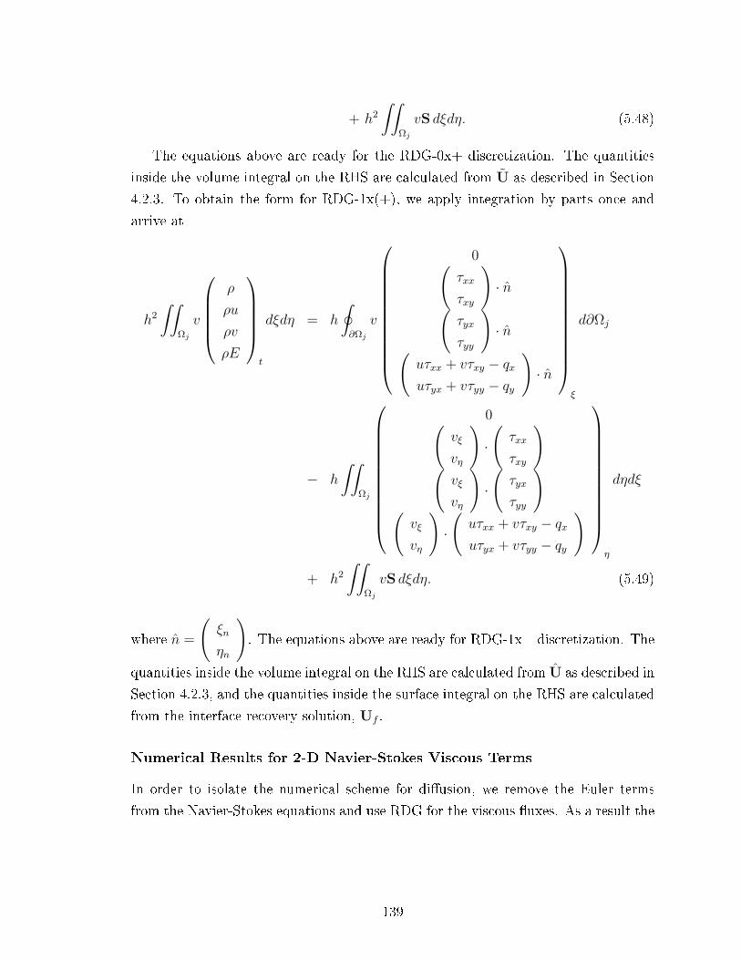
+ h2
∫∫Ωj
vS dξdη. (5.48)
The equations above are ready for the RDG-0x+ discretization. The quantities
inside the volume integral on the RHS are calculated from U as described in Section
4.2.3. To obtain the form for RDG-1x(+), we apply integration by parts once and
arrive at
h2
∫∫Ωj
v
ρ
ρu
ρv
ρE
t
dξdη = h
∮∂Ωj
v
0(τxx
τxy
)· n(
τyx
τyy
)· n(
uτxx + vτxy − qxuτyx + vτyy − qy
)· n
ξ
d∂Ωj
− h
∫∫Ωj
0(vξ
vη
)·(τxx
τxy
)(vξ
vη
)·(τyx
τyy
)(vξ
vη
)·(uτxx + vτxy − qxuτyx + vτyy − qy
)
η
dηdξ
+ h2
∫∫Ωj
vS dξdη. (5.49)
where n =
(ξn
ηn
). The equations above are ready for RDG-1x+ discretization. The
quantities inside the volume integral on the RHS are calculated from U as described in
Section 4.2.3, and the quantities inside the surface integral on the RHS are calculated
from the interface recovery solution, Uf .
Numerical Results for 2-D Navier-Stokes Viscous Terms
In order to isolate the numerical scheme for diusion, we remove the Euler terms
from the Navier-Stokes equations and use RDG for the viscous uxes. As a result the
139

density equation drops out resulting in the following system: ρu
ρv
ρE
t
=
τxx
τyx
uτxx + vτxy − qx
x
+
τxy
τyy
uτyx + vτyy − qy
y
, (5.50)
Our numerical test case is for a manufactured solution with approximate physics;
therefore, the values of the physical constants (such as Prandtl number, gas constant,
and specic-heat ratio) are xed. The simplied equations are as follows. The shear
stresses with Stokes' hypothesis are
τxx =2
3µ (2ux − vy) , (5.51)
τyy =2
3µ (2vy − vx) , (5.52)
τxy = τyx = µ (uy + vx) , (5.53)
and the heat uxes are,
qx =19
4µ
(P
ρ
)x
, (5.54)
qy =19
4µ
(P
ρ
)y
. (5.55)
We use a viscousity coecient similar to that of Sutherland's law,
µ =
(2
T + 1
)T
32 , (5.56)
where T is the temperature from the ideal gas law, p = ρRT , with R = 1. We
consider the following manufactured solutions,
ρ = U0 (x, y, t) = 2, (5.57)
ρu = U1 (x, y, t) = sin (2πx) sin (2πy) e−t, (5.58)
ρv = U2 (x, y, t) = sin (2πx) sin (2πy) e−t, (5.59)
ρE = U3 (x, y, t) = 5+sin (2πx) sin (2πy) e−t, (5.60)
and generate the appropriate source terms with Mathematica. We consider a periodic-
boundary unit-square domain with x ∈ [0, 1] and y ∈ [0, 1]. The RDG spatial dis-
cretizations are coupled with the 3rd-, 4th-, and 5th-order explicit Runge-Kutta tem-
140
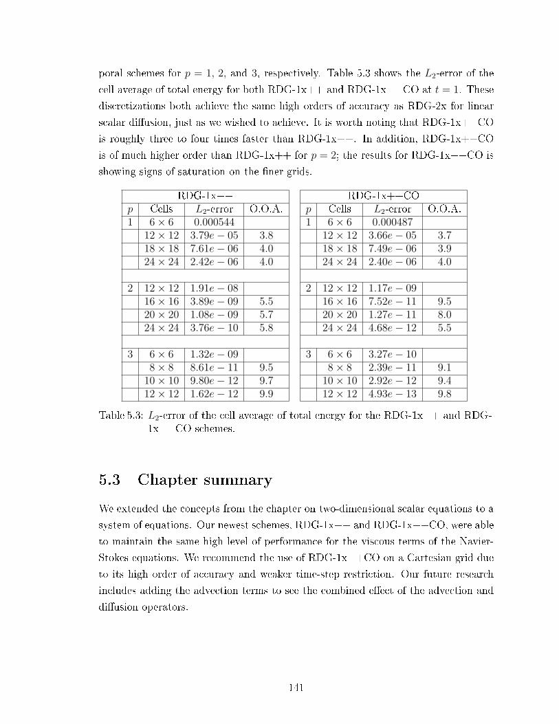
poral schemes for p = 1, 2, and 3, respectively. Table 5.3 shows the L2-error of the
cell average of total energy for both RDG-1x++ and RDG-1x++CO at t = 1. These
discretizations both achieve the same high orders of accuracy as RDG-2x for linear
scalar diusion, just as we wished to achieve. It is worth noting that RDG-1x++CO
is roughly three to four times faster than RDG-1x++. In addition, RDG-1x++CO
is of much higher order than RDG-1x++ for p = 2; the results for RDG-1x++CO is
showing signs of saturation on the ner grids.
RDG-1x++ RDG-1x++COp Cells L2-error O.O.A. p Cells L2-error O.O.A.1 6× 6 0.000544 1 6× 6 0.000487
12× 12 3.79e− 05 3.8 12× 12 3.66e− 05 3.718× 18 7.61e− 06 4.0 18× 18 7.49e− 06 3.924× 24 2.42e− 06 4.0 24× 24 2.40e− 06 4.0
2 12× 12 1.91e− 08 2 12× 12 1.17e− 0916× 16 3.89e− 09 5.5 16× 16 7.52e− 11 9.520× 20 1.08e− 09 5.7 20× 20 1.27e− 11 8.024× 24 3.76e− 10 5.8 24× 24 4.68e− 12 5.5
3 6× 6 1.32e− 09 3 6× 6 3.27e− 108× 8 8.61e− 11 9.5 8× 8 2.39e− 11 9.1
10× 10 9.80e− 12 9.7 10× 10 2.92e− 12 9.412× 12 1.62e− 12 9.9 12× 12 4.93e− 13 9.8
Table 5.3: L2-error of the cell average of total energy for the RDG-1x++ and RDG-1x++CO schemes.
5.3 Chapter summary
We extended the concepts from the chapter on two-dimensional scalar equations to a
system of equations. Our newest schemes, RDG-1x++ and RDG-1x++CO, were able
to maintain the same high level of performance for the viscous terms of the Navier-
Stokes equations. We recommend the use of RDG-1x++CO on a Cartesian grid due
to its high order of accuracy and weaker time-step restriction. Our future research
includes adding the advection terms to see the combined eect of the advection and
diusion operators.
141

CHAPTER VI
Hancock-Huynh Discontinuous
Galerkin Method
The discontinuous Galerkin method (DG) is well known for its ability to handle com-
plicated geometries, to achieve high eciency on parallel machines, and to obtain an
arbitrarily high order of accuracy. The method was introduced as a spatial discretiza-
tion that increases the order of spatial accuracy by adding more information per cell.
In 1973 Reed and Hill [32] demonstrated the spatial accuracy of DG schemes for
steady-state problems; however, the way to implement an equally high-order tempo-
ral discretization for time-accurate problems remained an enigma until much later. In
1989 Shu and Cockburn[7] successfully coupled the then popular Runge-Kutta method
with DG, thus introducing the rst successful high-order time-accurate DG scheme,
the Runge-Kutta discontinus Galerkin method (RK-DG). RK-DG is a semi-discrete
method where the temporal and spatial discretizations are completely decoupled,
therefore allowing the coding process to be modularized and CFD-algorithm devel-
opers to focus on just the spatial discretization. In simple language, RK advances in
time by making a number of estimates of the solution (or stages) in the course of one
time step, and then combining all of the estimates to take one full time step forward.
Despite the elegance of the seperation of spatial and temporal discretization, RK-DG
is not ecient due to the rapidly increasing number of stages needed for orders greater
than 4, and the reduction in stability domain caused by the hidden increase in stencil
size for one stage within the method.
Ruuth[35] introduced a special class of optimized RK schemes called Strong-
Stability-Preserving Runge-Kutta (SSP-RK), and Gottlieb[16] showcased a fth order
SSP-RK scheme consisting of 9 stages with Courant-Frierich-Lewy number (CFL) of
2.69. Ruuth and Gottlieb showed that increasing the number of stages also increases
142

the CFL number. The extension to a high order SS-PRK is not automatic; imple-
mentation requires strict adherence to the massive tables of coecients provided by
the papers mentioned above. Perhaps the most disturbing aspect of this special class
of RK methods is the lack of consideration for real engineering problems; the ux
evaluation in each stage can be so expensive that it osets the gain in CFL number.
We learn from this case that it is both the CFL and the number of ux evaluations
that determine the quality of a temporal scheme.
Lörcher, Gassner, and Munz[24] introduced an arbitrary high-order space-time ex-
pansion (STE-DG) method. The process of going to a higher order is fully automatic
and the scheme allows for local time stepping. In a global time-stepping scheme like
RK-DG, the time step is restricted by the smallest cell in the computational grid. A
local time-stepping scheme allows each cell to take multiple timesteps of dierent size,
hence signicantly increasing the computational eciency. Unlike RK-DG, STE-DG
suers a CFL reduction as the order of the solution polynomial increases, making it
worse than RK-DG on uniform grids. Recently Huynh[18] revisited Van Leer's[37]
scheme III and developed the moment scheme. The moment scheme is strictly for
p = 1 and it is for hyperbolic equations only. To avoid confusion with other uses of
the word moment, the name Hancock-Huynh DG (HH-DG) will be used.
A new generation of space-time methods is evolving from Hancock's observation
and will be discussed in detail in the next section. Our research goal is to apply Han-
cock's observation and extend Huynh's moment scheme beyond p = 1. In addition,
we want to extend these concepts to diusion!
The key component of the new generation of DG schemes is to integrate the gov-
erning equation in both space and time. Since the integration is over both time and
space, the temporal and spatial discretizations are no longer seperate! In this regard,
the original solution must be modied to contain the time variable. Both HH-DG and
STE-DG acquire a space-time expanded solution from the purely spatial initial dis-
cretization of the solution. The space-time expanded solution contains both temporal
and spatial derivatives, which provides a complete estimate of the solution at later
times. Traditionally, the space-time expansion is done with Cauchy-Kovalevasakya
(CK) procedure, which is used in STE-DG. CK is an exact analytical procedure for
determining temporal derivatives from the spatial derivatives based on the governing
equations. However, the overhead for determining a space-time expanded solution
might cost more than a few ux evaluations, making it computationally expensive.
Huynh proposed a cost-ecient way to acquire the space-time expanded solution
based on a local Runge-Kutta method (LRK), which can be viewed as a numerical
143

version of the CK procedure.
This chapter begins by reviewing Hancock's observation, which is then followed
by three main sections: HH-DG for the advection operator, HH-DG for the diusion
operator, and HH-DG for the combined advection and diusion operators. The ad-
vection section is presented rst due to its simplicity; we want the HH-DG advection
operator to mimic the exact shift operator. Within this section we cover the numeri-
cal techniques for acquiring the space-time expanded solution via the LRK procedure,
and most importantly, the accurate evaluation of space-time integrals.
6.1 Hancock's Observation
In 1971 Steve Hancock1 made an important observation regarding upwind schemes
for hyperbolic equations, leading to the most ecient implementation of the second-
order, Godunov-type MUSCL scheme[38]. The observation is illustrated in Figure
6.1, an (x, t)-diagram for the Euler equations showing cell Ωj and neighbors Ωj±1. In
an upwind nite-volume scheme the upwind bias comes from computing the interface
uxes with the Backward Method of Characteristics. The diagram shows the charac-
teristics drawn backward in time from each interface starting at time tn+τ . The ow
in this region is assumed to be subsonic in the positive direction, so there are two for-
ward characteristics and a backward one. It is seen that at interface xj− 12the forward
characteristics bring information from cell Ωj−1 to the interface, while the backward
characteristic brings information from cell Ωj. Similarly, at interface xj+ 12the forward
characteristics bring information from Ωj, while the backward characteristic brings
information from Ωj+1.
This description stems from an interface-centered mindset. Hancock noticed that,
if we switch to a cell-centered point of view, we see that inside cell Ωj all three
characteristic equations are used to update the solution to time-level tn + τ . These
form a complete set of ow equations; thus, we may as well use any other complete set
of ow equations to describe the evolution within this cell, for instance, conservative
or primitive rather than characteristic variables. Staying in the cell-centered mindset,
we may update the solution inside cell Ωj to time tn + τ using information from this
cell only, as if it had no neighbors, as if the (polynomial) initial-value distributions of
ow variables stretched beyond the cell. This is the core of Hancock's Observation.
Advancing the solution internally in all cells, in particular, in Ωj−1 and Ωj+1,
creates a discontinuity at each interface, in particular, at xj− 12and xj+ 1
2. At time
1Then at Physics International, Hayward, CA.
144

Ωj
t
Ωj - 1xj-½
xj+½ Ωj + 1
τ
−Γj
0
1−Γj
+
−Γ
1j
−Γj+1
0Γj
+Γj
Figure 6.1: Hancock observes that the waves generated from the local evolution oftwo elements, Ωj and Ωj+1, result in the correct waves arriving at theelement interface centered on xj+ 1
2.
tn + τ a unique ux vector may obtained at each interface by applying a Riemann
solver to each discontinuity; this makes the ux upwind-biased. Hancock made his
observation for a scheme with linear subcell data obtained by interpolation (a nite-
volume method with p = 1); in this case an upwind ux computed at tn+ 12∆t suces
to update the conserved quantities to time tn+∆t with second-order accuracy. When
applying this scheme to linear advection the upwind-biased Fromm scheme[13], the
nite-volume version of Van Leer's Scheme III, appears.
Hancock's formulation of the p = 1 scheme was the rst STE scheme avant la
lettre. When making Hancock's Observation for an upwind-biased scheme of a higher
order, it follows that Riemann uxes are needed at various times with τ ≤ ∆t, in
order to compute a more accurate time-integral of the ux; as we shall see below,
this is precisely the STE method, whether a nite-volume or a DG discretization is
considered. It appears that Lörcher et al. were not aware of Hancock's version of
MUSCL, or did not recognize its signicance.
It is the merit of Huynh to have realized that for a space-time DG method to
achieve superior accuracy and stability, the space-time volume integral must also be
subjected to the inuence of neighboring cells, rather than being computed solely
from the interior STE solution.
We are now ready to discuss in detail the discretization of the space-time weak
equations.
145
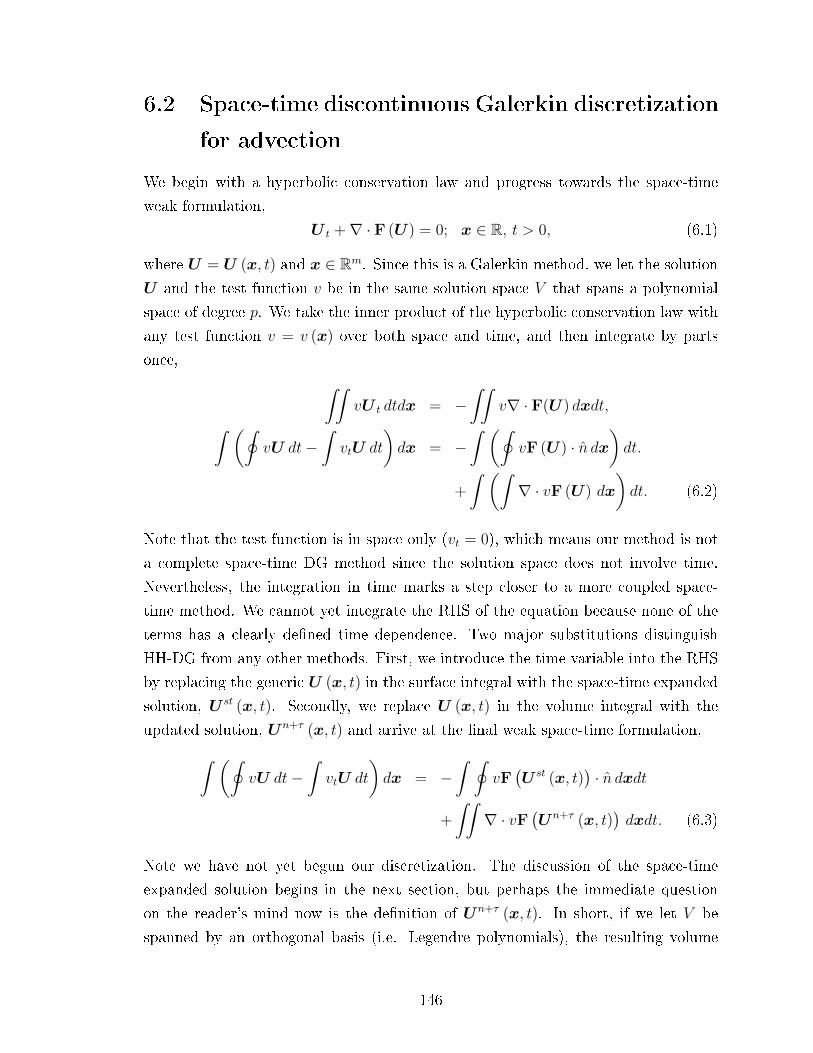
6.2 Space-time discontinuous Galerkin discretization
for advection
We begin with a hyperbolic conservation law and progress towards the space-time
weak formulation,
U t +∇ · F (U) = 0; x ∈ R, t > 0, (6.1)
where U = U (x, t) and x ∈ Rm. Since this is a Galerkin method, we let the solution
U and the test function v be in the same solution space V that spans a polynomial
space of degree p. We take the inner product of the hyperbolic conservation law with
any test function v = v (x) over both space and time, and then integrate by parts
once, ∫∫vU t dtdx = −
∫∫v∇ · F(U) dxdt,∫ (∮
vU dt−∫vtU dt
)dx = −
∫ (∮vF (U ) · n dx
)dt.
+
∫ (∫∇ · vF (U ) dx
)dt. (6.2)
Note that the test function is in space only (vt = 0), which means our method is not
a complete space-time DG method since the solution space does not involve time.
Nevertheless, the integration in time marks a step closer to a more coupled space-
time method. We cannot yet integrate the RHS of the equation because none of the
terms has a clearly dened time dependence. Two major substitutions distinguish
HH-DG from any other methods. First, we introduce the time variable into the RHS
by replacing the generic U (x, t) in the surface integral with the space-time expanded
solution, U st (x, t). Secondly, we replace U (x, t) in the volume integral with the
updated solution, Un+τ (x, t) and arrive at the nal weak space-time formulation,∫ (∮vU dt−
∫vtU dt
)dx = −
∫ ∮vF(U st (x, t)
)· n dxdt
+
∫∫∇ · vF
(Un+τ (x, t)
)dxdt. (6.3)
Note we have not yet begun our discretization. The discussion of the space-time
expanded solution begins in the next section, but perhaps the immediate question
on the reader's mind now is the denition of Un+τ (x, t). In short, if we let V be
spanned by an orthogonal basis (i.e. Legendre polynomials), the resulting volume
146
integral in the RHS of Eqn 6.3 becomes explicit. The update equation for the zeroth
moment does not contain a volume integral, hence the zeroth moment is rst updated.
The update equation for the rst gradient will use the newest result from the zeroth
moment. The choice of an orthogonal basis creates a hierarchical structure in which
the update equation of the n-th moment depends on the solution of the (n− 1)-th or
lower moments. This will also be explained in detail in the next section.
6.2.1 One-dimension linear advection
We begin with the simplest equation to demonstrate the discretization of the RHS of
Eqn 6.3. Consider the scalar linear advection equation,
ut + aux = 0; x ∈ R, t > 0. (6.4)
For element Ωj with x ∈[xj− 1
2, xj+ 1
2
]and at time t = tn, the transformation to local
coordinates in both space and time reads,
ξ =x− xj− 1
2
∆x,
τ =t− tn
∆t, (6.5)
with both ξ, τ ∈ [0, 1]. We acquire the space-time DG formulation by taking the inner
product of Eqn(6.4) with a test function v (ξ) and integrate by parts over element Ωj,
∆x
∫ (∮vu dτ
)dξ = −a∆t
∫ (∮vu · n dξ −
∫vξu dξ
)dτ,
∆x
∫v(un+1 − un
)dξ = −a∆t
∫ (vu |ξ=1 −vu |ξ=0 −
∫vξu dξ
)dτ,
We isolate the unknown un+1 on the LHS,∫vun+1dξ =
∫vundξ − a∆t
∆x
∫ (vu |ξ=1 −vu |ξ=0 −
∫vξu dξ
)dτ. (6.6)
In the RHS, un is simply the old solution, while the solutions in the surface and
volume integrals are yet to be dened. We now introduce a space-time expanded
solution ust, as a replacement for u in the surface integral and the updated solution
147
un+τ , as a replacement of u in the volume integral,∫vun+1dξ =
∫vundξ − a∆t
∆x
∫ (vust |ξ=1 −vust |ξ=0 −
∫vξu
n+τ dξ
)dτ. (6.7)
Our goal for the advection operator is to mimic the exact shift operator, which is
a highly desirable property when solving for advection-dominated problems. This
minimizes dissipation and dispersive errors, ensuring accurate propagation of waves
over long distances. We shall discuss the exact shift operator for advection, and then
design ust and un+τ to mimic its behavior.
Exact shift operator for DG in 1-D
The term shift refers to the solution being advected over a nite distance; the term
exact remains ambiguous at this moment. In order to clarify this ambiguity, the
section is partitioned in two: the exact shift operator and the exact projected shift
operator. The Courant number is universally dened as
ν = adt
dx. (6.8)
The exact shift operator can only be numerically achieved with ν = 1; while for ν < 1,
an extra projection step must be applied to obtain the exact projected shift operator.
Exact shift operator
A numerical method that results in the exact shift operator when ν = 1 is certainly
desirable because such a method exhibits zero dissipation and phase error while ad-
vecting waves over long distance and time. For linear advection with a > 0, the
solution at a new time level is shifted to the right as shown in Figure 6.2. As a result,
the update equation is simply
un+1j = unj−1, a > 0. (6.9)
Exact Projected Shift Operator
When shifting the solution with ν < 1, the discontinuity between meshes Ωj and
Ωj−1 rests inside of Ωj. As a result, an extra projection step must be taken to get
the solution back into the space V . In this piecewise-linear (p = 1) example shown
148

Ωj Ωj + 1Ωj - 1
u
Figure 6.2: The exact shift operator occurs when ν = 1. The solution of Ωj att = t0 + ∆t is equal to the solution of Ωj−1 at t = t0.
in Figure 6.3, the dashed line indicates the location of the shift solution, ushiftedj . We
nd a new projected solution by enforcing for all v in V ,∫Ωj
vun+1j dx =
1
∆x
∫ΩA
vushiftedj dξ +1
∆x
∫ΩB
vushiftedj dx, (6.10)
where the intervals are dened in terms of local coordinate to be ΩA = [0 ν], and
ΩB = [ν 1]. Note that the result of this type of projection is no longer exact, but
this is the best one can achieved with a shift less than one mesh.
Ωj Ωj + 1Ωj - 1
u
Figure 6.3: For ν < 1, the subcell shift causes the original discontinuity at the inter-face to be shifted to the interior of Ωj. The new solution of Ωj (dotted
line) is now acquired by projecting the discontinuous solution ushiftedj intothe solution space.
149
Example of shift operators in matrix form
In this simple example, we show the exact projected shift operator for a > 0 up to
p = 2. The new solution of Ωj at t = t0 + ∆t is a linear combination of the old
solution of Ωj−1 and Ωj at t = t0,
ut0+∆tj = MLu
t0j−1 + MCut0j , (6.11)
where u is a column vector of coecients of u starting with the lowest moment from
top to bottom. The solution u is spanned by the orthogonal Legendre polynomials,
u = u+ ∆u (2ξ − 1) + ∆2u(6ξ2 − 6ξ + 1
). (6.12)
The exact projected-shift matrices ML and MC are expressed below. For p = 0,
ML = [ν] , MC = [1− ν] . (6.13)
For p = 1,
ML =
[ν ν − ν2
−3ν + 3ν2 −3ν + 6ν2 − 2ν3
], MC =
[1− ν −v + v2
3ν − 3ν2 1− 3ν + 2ν3
].
(6.14)
For p = 2,
ML =
ν ν − ν2 ν − 3ν + 2ν3
−3ν + 3ν2 −3ν + 6ν2 − 2ν3 −3ν + 12ν2 − 12ν3 + 3ν4
5ν − 15ν2 + 10ν3 5ν − 20ν2 + 20ν3 − 5ν4 5ν − 30ν2 + 50ν3 − 30ν4 + 6ν5
,
MC =
1− ν −ν + ν2 −ν + 3ν − 2ν3
3ν − 3ν2 1− 3ν + 2ν3 −3ν + 6ν2 − 3ν4
−5ν + 15ν2 − 10ν3 5ν − 10ν2 + 5ν4 1− 5ν + 10ν3 − 6ν5
. (6.15)
Note that for ν = 1, MC becomes the zero matrix, and ML becomes the exact shift
operator. To the knowledge of the author, no time-marching method coupled with
DG spatial discretization for p ≥ 1 is stable with ν = 1, hence the exact shift operator
is rarely achieved in practice. We will soon show HH-DG is the exact projected shift
operator for ν < 1 and the exact shift operator for ν = 1. But before we get excited,
we rst dene the space-time expanded solution.
150
Space-time expanded solution
HH-DG treats the surface integral on the RHS with special care; the spatial solution
uj (ξ) is replaced with a space-time expanded solution ustj (ξ, τ). For the scalar linear-
advection equation, determining ustj via the Cauchy-Kovalevskaya (CK) procedure is
straightforward. First the solution is Taylor-expanded in both space and time (to
2nd-order in this example),
u (x, t) = uj + ux,j (x− xj) + ut,j (t− tn) +uxx,j
2(x− xj)2
+uxt,j (x− xj) (t− tn) +utt,j
2(t− tn)2 , (6.16)
and then the CK prodecure automatically express all temporal derivatives in terms
of spatial derivatives based on the governing equation. The higher order derivatives
in t are determined using a hierarchical procedure starting with the lowest order
derivative,
ut = −aux,utt = (−aux)t = a2uxx,
uxt = (ux)t = −auxx.
The CK procedure becomes extremely complicated for nonlinear systems of equa-
tions as experienced by Lörcher[24] while experimenting with STE-DG. The need
to solve for these space-time derivatives eciently means a numerical estimation is
preferred over an analytical one.
We introduce Huynh's approximation to ustj using a local Runge Kutta (LRK)
procedure. The term local implies Eqn (6.6) is solved by only considering the local
value of uj. Figure (6.4) reveals the denition of a local ux. The solution in Ωj
is assumed to extend beyond the element boundary in both directions, hence the
characteristic lines are continuous across the element interfaces. The solution on
the interface is now uniquely dened; therefore there is no need for an approximate
Riemann solver. LRK advances the solution to Radau points (see Appendix A) in
a sequential manner, and the solution at these Radau points are stored. Figure(6.4)
shows the location three Radau points of a HH-DG (p = 2) scheme.
Notice we only need to know the values of ustj at the element interfaces. We briey
discuss the technical details of the LRK procedure.
151

Ωj
u3=1.00
2=0.64
1=0.15
1st LL-RK
2nd LL-RK
3rd LL-RK
Chara
cteristic L
ines
Figure 6.4: HH-DG (p = 2) using local Runge-Kutta to obtain ust. Dashed lines in-dicates location of stored space-time solution values. The lightly dottedlines are characteristics from Ωj and they illustrate an important propertyof locality. For LRK, these characteristics are assumed to be valid out-side of Ωj, hence the function values of u on the boundaries are uniquelydened.
Local linear Runge-Kutta
From our numerical experiments we discovered a linear LRK (LL-RK) procedure is
sucient for the determination of space-time derivatives for both linear and nonlinear
governing equations. A linear RK scheme is very low on storage requirement, and
the use of local uxes makes it extremely economical. The K-th order linear RK
scheme for a system of variables comes from the nested expansion of eλt, where λ is
the eigenvalue of the spatial operator,
U (1) = Un +∆t
KRes (Un) ,
U (2) = Un +∆t
K − 1Res
(U (1)
),
...
U (i) = Un +∆t
K − i+ 1Res
(U (i−1)
),
...
U (K) = Un +∆t
1Res
(U (K−1)
), (6.17)
152
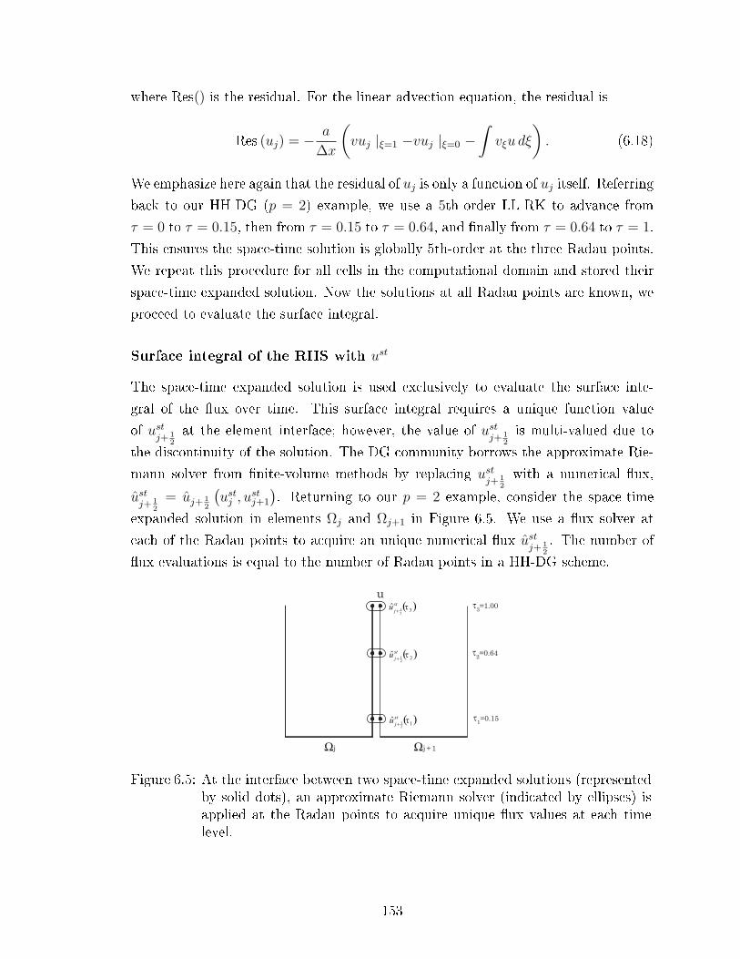
where Res() is the residual. For the linear advection equation, the residual is
Res (uj) = − a
∆x
(vuj |ξ=1 −vuj |ξ=0 −
∫vξu dξ
). (6.18)
We emphasize here again that the residual of uj is only a function of uj itself. Referring
back to our HH-DG (p = 2) example, we use a 5th-order LL-RK to advance from
τ = 0 to τ = 0.15, then from τ = 0.15 to τ = 0.64, and nally from τ = 0.64 to τ = 1.
This ensures the space-time solution is globally 5th-order at the three Radau points.
We repeat this procedure for all cells in the computational domain and stored their
space-time expanded solution. Now the solutions at all Radau points are known, we
proceed to evaluate the surface integral.
Surface integral of the RHS with ust
The space-time expanded solution is used exclusively to evaluate the surface inte-
gral of the ux over time. This surface integral requires a unique function value
of ustj+ 1
2
at the element interface; however, the value of ustj+ 1
2
is multi-valued due to
the discontinuity of the solution. The DG community borrows the approximate Rie-
mann solver from nite-volume methods by replacing ustj+ 1
2
with a numerical ux,
ustj+ 1
2
= uj+ 12
(ustj , u
stj+1
). Returning to our p = 2 example, consider the space-time
expanded solution in elements Ωj and Ωj+1 in Figure 6.5. We use a ux solver at
each of the Radau points to acquire an unique numerical ux ustj+ 1
2
. The number of
ux evaluations is equal to the number of Radau points in a HH-DG scheme.
Ωj + 1
u
Ωj
( )3
2
1ˆ τst
ju
+
3=1.00
2=0.64
1=0.15 ( )
12
1ˆ τst
ju
+
( )2
2
1ˆ τst
ju
+
Figure 6.5: At the interface between two space-time expanded solutions (representedby solid dots), an approximate Riemann solver (indicated by ellipses) isapplied at the Radau points to acquire unique ux values at each timelevel.
153

We use the upwind ux for linear advection with a > 0,
uj+ 12
= ustj (ξ = 1, τ) . (6.19)
Applying this to Eqn.(6.6) results in
∫vun+1dξ =
∫vundξ − a∆t
∆x
∫ (v (1)ustj (ξ = 1, τ)− v (0)ustj−1 (ξ = 1, τ))dτ︸ ︷︷ ︸
surface integral
+a∆t
∆x
∫∫ vξun+τj dξdτ︸ ︷︷ ︸
volume integral
. (6.20)
The last component to be discussed is the volume integral. In addition, we shall
discuss a numerical technique to integrate in time based on the Radau points.
Volume integral of RHS based on un+τj
The correct evaluation of the volume integral in Eqn (6.20) is essential for high-order
accuracy. In the volume integral of STE-DG, un+τj is simply taken as ustj ; this results
in a lower-order scheme with severely restricted CFL number. The use of ustj in the
volume integral implies no information with neighboring elements penetrates into the
interior of Ωj; the omission of wave interaction from neighboring elements results in
inaccurate physics. The HH-DG scheme takes advantage of the orthogonality of the
Legendre polynomials and incorporates wave interaction into the volume integral by
using the newest solution available. Let us illustrate this through a p = 3 example';
consider u at t = tn to be constructed out of Legendre polynomials up to the cubic
component,
v0 = 1,
v1 = 2ξ − 1,
v2 = 6ξ2 − 6ξ + 1,
154

v3 = 20ξ3 − 30ξ2 + 12ξ + 1,
unj (ξ) = u v0 + ∆u v1 + ∆2u v2 + ∆3uv3, (6.21)
where u, ∆u, ∆2u, and ∆3u are the cell average, rst average gradient, second average
gradient and third average gradient, respectively. The nal update equations are
un+τ = un − a∆t
∆x
∫ τ
0
(ustj (1, τ)− ustj (0, τ)
)dτ, (6.22)
∆un+τ
= ∆un − 3a∆t
∆x
∫ τ
0
(ustj (1, τ) + ustj (0, τ)
)dτ
+3a∆t
∆x
∫ τ
0
2un+τdτ, (6.23)
∆2un+τ
= ∆2un − 5a∆t
∆x
∫ τ
0
(ustj (1, τ)− ustj (0, τ)
)dτ
+5a∆t
∆x
∫ τ
0
2∆un+τ
dτ, (6.24)
∆3un+τ
= ∆3un − 7a∆t
∆x
∫ τ
0
(ustj (1, τ) + ustj (0, τ)
)dτ
+7a∆t
∆x
∫ τ
0
(2un+τ + 2∆2u
n+τ)dτ. (6.25)
Our obvious goal is to nd the solution at τ = 1, but that is not so straightforward
for the gradients. With our specic choice of orthogonal basis, the update equation
for u is a stand-alone equation that can be solved rst. Next, we consider the update
equation for ∆u where the volume integral on the RHS requires us to know un+τ
at the Radau points. In other words, we need to solve the update equation of u
at various Radau points to update ∆u. Sequentially, we need to solve the update
equation of ∆u at various Radau points to update ∆2u. This hierachical structure
for updating variables is the strategy employed in HH-DG to include wave interaction
into the volume integral. The integration of the surface and volume integrals in time
may seem expensive; in this regard, we introduce a numerical trick called implicit
155

Radau integration in Appendix A to reduce the computational cost.
The current HH-DG scheme with Legendre polynomial is explicit in time. If we
are to use a non-orthogonal basis, the volume integral will include other solution
coecients, turning HH-DG into an implicit scheme. This would imply an extra
nonlinear solver must be implemented; the study on the cost and accuracy of using
non-orthogonal basis is left for the future.
Numerical results for linear advection
The following numerical example takes a = 1 on the domain x ∈ [0, 1], with periodic
boundary condition. The initial values form a sine wave,
U0 = sin(2πx). (6.26)
The ending time is a positive integer, hence the exact nal solution is the same as the
initial values. For both HH-DG and STE-DG with p-th order solution polynomial,
the code uses a (p+ 1)-point Radau-Gaussian integration in time, and a (2p+ 1)-
point Gaussian integration in space. A comparison between STE-DG and HH-DG for
p = 1 is provided in Table 6.1. HH-DG is clearly faster due to the larger time step;
in this case the CFL number achieved by HH-DG is more than 3 times larger. In
reality, HH-DG is able to achieve a CFL of unity, which results in the exact solution
due to the exact-shift property; however, we refrained from doing that in order to get
a measurement of the order of accuracy.
We then consider advecting waves over a long period of time, tmax = 300. Table
6.2 shows the order of accuracy is clearly 2p+ 1 in the cell average, whereas the order
of accuracy of the rst average gradient is quite unpredictable. Again the CFL is set
to 0.9375 because there is no numerical error with a CFL of unity.
Brief remark on stability analysis
The Fourier analysis for stability is omitted for the HH-DG advection operator for
one good reason. It turns out the nal update matrix for the scalar linear advec-
tion equation is simply given by the exact shift and exact projected shift operators
presented in the previous section. As long as ν ≤ 1, stability is ensured.
156
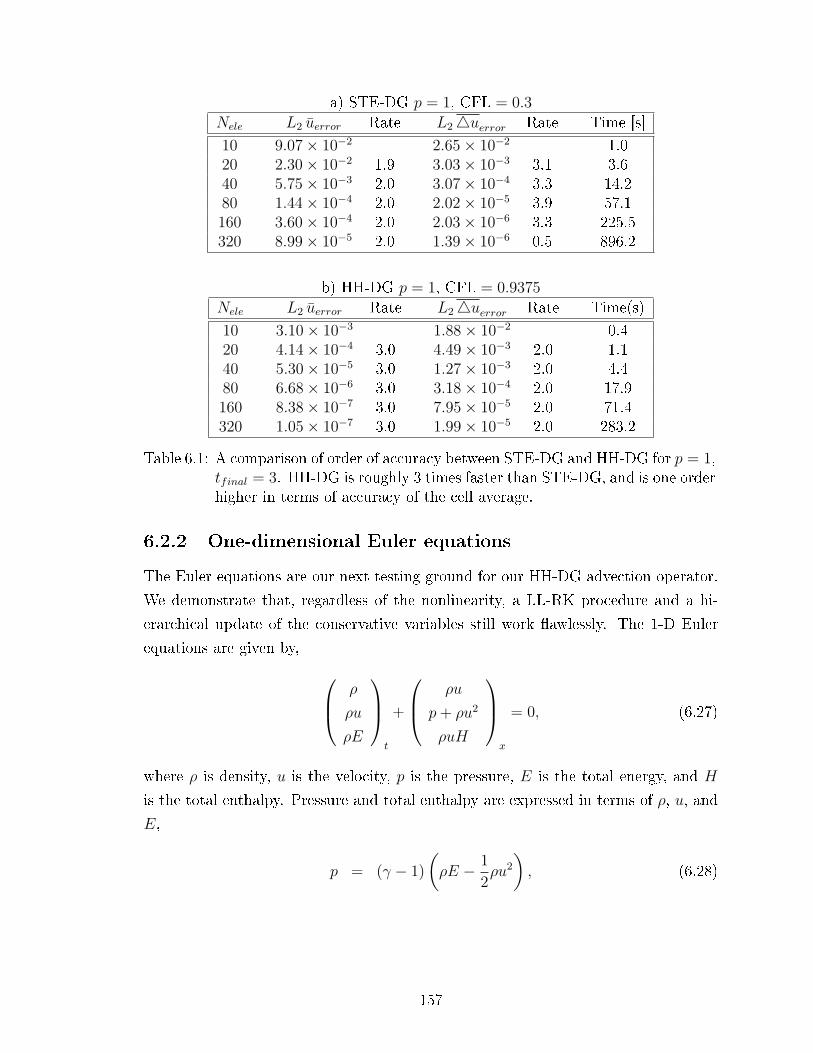
a) STE-DG p = 1, CFL = 0.3
Nele L2 uerror Rate L24uerror Rate Time [s]
10 9.07× 10⁻² 2.65× 10⁻² 1.020 2.30× 10⁻² 1.9 3.03× 10⁻³ 3.1 3.640 5.75× 10⁻³ 2.0 3.07× 10⁻⁴ 3.3 14.280 1.44× 10⁻⁴ 2.0 2.02× 10⁻⁵ 3.9 57.1160 3.60× 10⁻⁴ 2.0 2.03× 10⁻⁶ 3.3 225.5320 8.99× 10⁻⁵ 2.0 1.39× 10⁻⁶ 0.5 896.2
b) HH-DG p = 1, CFL = 0.9375
Nele L2 uerror Rate L24uerror Rate Time(s)
10 3.10× 10⁻³ 1.88× 10⁻² 0.420 4.14× 10⁻⁴ 3.0 4.49× 10⁻³ 2.0 1.140 5.30× 10⁻⁵ 3.0 1.27× 10⁻³ 2.0 4.480 6.68× 10⁻⁶ 3.0 3.18× 10⁻⁴ 2.0 17.9160 8.38× 10⁻⁷ 3.0 7.95× 10⁻⁵ 2.0 71.4320 1.05× 10⁻⁷ 3.0 1.99× 10⁻⁵ 2.0 283.2
Table 6.1: A comparison of order of accuracy between STE-DG and HH-DG for p = 1,tfinal = 3. HH-DG is roughly 3 times faster than STE-DG, and is one orderhigher in terms of accuracy of the cell average.
6.2.2 One-dimensional Euler equations
The Euler equations are our next testing ground for our HH-DG advection operator.
We demonstrate that, regardless of the nonlinearity, a LL-RK procedure and a hi-
erarchical update of the conservative variables still work awlessly. The 1-D Euler
equations are given by, ρ
ρu
ρE
t
+
ρu
p+ ρu2
ρuH
x
= 0, (6.27)
where ρ is density, u is the velocity, p is the pressure, E is the total energy, and H
is the total enthalpy. Pressure and total enthalpy are expressed in terms of ρ, u, and
E,
p = (γ − 1)
(ρE − 1
2ρu2
), (6.28)
157

a) HH-DG p = 1
Nele L2 uerror Rate L24uerror Rate
10 4.01× 10⁻² 1.80× 10⁻²
20 5.28× 10⁻³ 2.9 1.88× 10⁻³ 3.340 6.71× 10⁻⁴ 3.0 6.25× 10⁻⁴ 1.680 8.40× 10⁻⁵ 3.0 2.66× 10⁻⁴ 1.2160 1.05× 10⁻⁵ 3.0 2.09× 10⁻⁵ 3.7320 1.31× 10⁻⁶ 3.0 1.37× 10⁻⁵ 0.6
b) HH-DG p = 2
Nele L2 uerror Rate L24uerror Rate L242uerror Rate
10 9.61× 10⁻⁴ 2.96× 10⁻⁴ 1.20× 10⁻³
20 3.08× 10⁻⁵ 5.0 5.15× 10⁻⁶ 5.8 1.50× 10⁻⁴ 3.040 9.73× 10⁻⁷ 5.0 3.21× 10⁻⁷ 4.0 1.87× 10⁻⁵ 3.080 3.07× 10⁻⁸ 5.0 3.45× 10⁻⁸ 3.2 2.34× 10⁻⁶ 3.0160 9.71× 10⁻¹⁰ 5.0 4.03× 10⁻⁹ 3.1 2.93× 10⁻⁷ 3.0320 3.12× 10⁻¹¹ 5.0 4.92× 10⁻¹⁰ 3.0 3.66× 10⁻⁸ 3.0
b) HH-DG p = 3
Nele L2 uerror Rate L24uerror Rate
10 5.58× 10⁻⁶ 1.75× 10⁻⁶
20 4.50× 10⁻⁸ 7.0 5.86× 10⁻⁸ 4.940 3.69× 10⁻¹⁰ 6.9 3.64× 10⁻⁹ 4.080 4.13× 10⁻¹² 6.5 2.27× 10⁻¹⁰ 4.0160 1.23× 10⁻¹³ 5.1 1.42× 10⁻¹¹ 4.0
Nele L242uerror Rate L243uerror Rate
10 2.75× 10⁻⁶ 4.92× 10⁻⁵
20 8.68× 10⁻⁸ 4.9 3.08× 10⁻⁶ 4.040 2.72× 10⁻⁹ 5.0 1.92× 10⁻⁷ 4.080 8.51× 10⁻¹¹ 5.0 1.20× 10⁻⁸ 4.0160 2.66× 10⁻¹² 5.0 7.51× 10⁻¹⁰ 4.0
Table 6.2: Order of accuracy for p = 1, 2, 3, CFL = 0.9375, tfinal = 300.
158

H = E +p
ρ. (6.29)
The primitive variables are replaced with the conservative variables,
U t +∇ · F (U) =
U0
U1
U2
t
+
U1
p+U2
1
U0
U1H
x
= 0, (6.30)
where p and H is now,
p = (γ − 1)
(U2 −
U21
2U0
), (6.31)
H =U1
U0
(U2 + (γ − 1)
(U2 −
U21
2U0
)). (6.32)
We transform the conservative form of the Euler equations into weak form as with
Eqn 6.3,∫vUn+1dξ =
∫vUndξ +
∆t
∆x
∫vξF
(Un+τj
)dξdτ
−∆t
∆x
(∫ (v (1) F
(U stj (1, τ)
)− v (0) F
(U stj−1 (1, τ)
))dτ
)(6.33)
We acquire U stj−1 by using a suitable order of LL-RK, and then solve the Riemann
problem at the various Radau points using an approximate Roe solver[33]. The real
enigma arises in the the volume integral of the RHS where the volume integrals for
momentum and total energy contain highly nonlinear terms that make it impossible
to express Un+τj solely in terms of the updated variables. Our solution is to express
F(Un+τj
)in terms of both updated variables Un+τ
j , and the space-time expanded
solution, U stj−1. The following examples for p = 1 and 2 shall kindly supplement your
understanding.
159

1-D Euler HH-DG p = 1 discretization
The piecewise-linear orthogonal Legendre basis is given by
v0 = 1,
v1 = 2ξ − 1. ξ ∈ [0, 1]
The three conservative variables are expressed as
U0 = U0 + ∆U0 (2ξ − 1) ,
U1 = U1 + ∆U1 (2ξ − 1) ,
U2 = U2 + ∆U2 (2ξ − 1) ,
summing up to a total of six degrees of freedom per element. We churn out the update
equations by inserting these expressions into Eqn 6.33,
Un+τ
= Un − ∆t
∆x
(∫ τ
0
(Fj+ 1
2− Fj− 1
2
)dτ
), (6.34)
∆Un+τ
= ∆Un − 3∆t
∆x
(∫ τ
0
(Fj+ 1
2+ Fj− 1
2
)dτ
)+
3∆t
∆x
(∫∫ τ
0
v1 (ξ) F(UHDGp1
)dτdξ
). (6.35)
Notice the same∫ τ
0Fj+ 1
2dτ is used in both update equations. We rst use a LL-RK
procedure to acquire U stj (ξ, τk) at all Radau points τk,
U st (ξ, τk) =
U0st,τk
+ ∆U0st,τk
(2ξ − 1)
U1st,τk
+ ∆U1st,τk
(2ξ − 1)
U2st,τk
+ ∆U2st,τk
(2ξ − 1)
. (6.36)
The space-time expanded solutions are then fed into a numerical ux solver,
Fτkj+ 1
2
= Fτkj+ 1
2
(U stj (1, τk) ,U
stj+1 (0, τk)
). (6.37)
We solve for the ux at all Radau points to integrate∫ τ
0Fj+ 1
2dτ numerically. Eqn 6.34
is easily solved to provide the new cell averages at the Radau points. As for updating
160
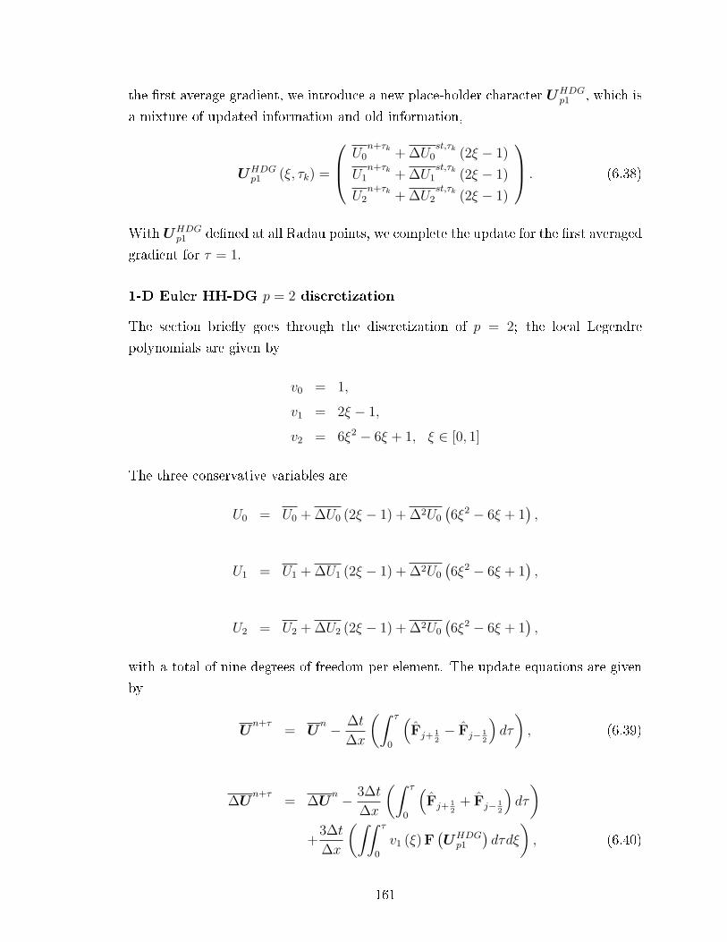
the rst average gradient, we introduce a new place-holder character UHDGp1 , which is
a mixture of updated information and old information,
UHDGp1 (ξ, τk) =
U0n+τk
+ ∆U0st,τk
(2ξ − 1)
U1n+τk
+ ∆U1st,τk
(2ξ − 1)
U2n+τk
+ ∆U2st,τk
(2ξ − 1)
. (6.38)
With UHDGp1 dened at all Radau points, we complete the update for the rst averaged
gradient for τ = 1.
1-D Euler HH-DG p = 2 discretization
The section briey goes through the discretization of p = 2; the local Legendre
polynomials are given by
v0 = 1,
v1 = 2ξ − 1,
v2 = 6ξ2 − 6ξ + 1, ξ ∈ [0, 1]
The three conservative variables are
U0 = U0 + ∆U0 (2ξ − 1) + ∆2U0
(6ξ2 − 6ξ + 1
),
U1 = U1 + ∆U1 (2ξ − 1) + ∆2U0
(6ξ2 − 6ξ + 1
),
U2 = U2 + ∆U2 (2ξ − 1) + ∆2U0
(6ξ2 − 6ξ + 1
),
with a total of nine degrees of freedom per element. The update equations are given
by
Un+τ
= Un − ∆t
∆x
(∫ τ
0
(Fj+ 1
2− Fj− 1
2
)dτ
), (6.39)
∆Un+τ
= ∆Un − 3∆t
∆x
(∫ τ
0
(Fj+ 1
2+ Fj− 1
2
)dτ
)+
3∆t
∆x
(∫∫ τ
0
v1 (ξ) F(UHDGp1
)dτdξ
), (6.40)
161
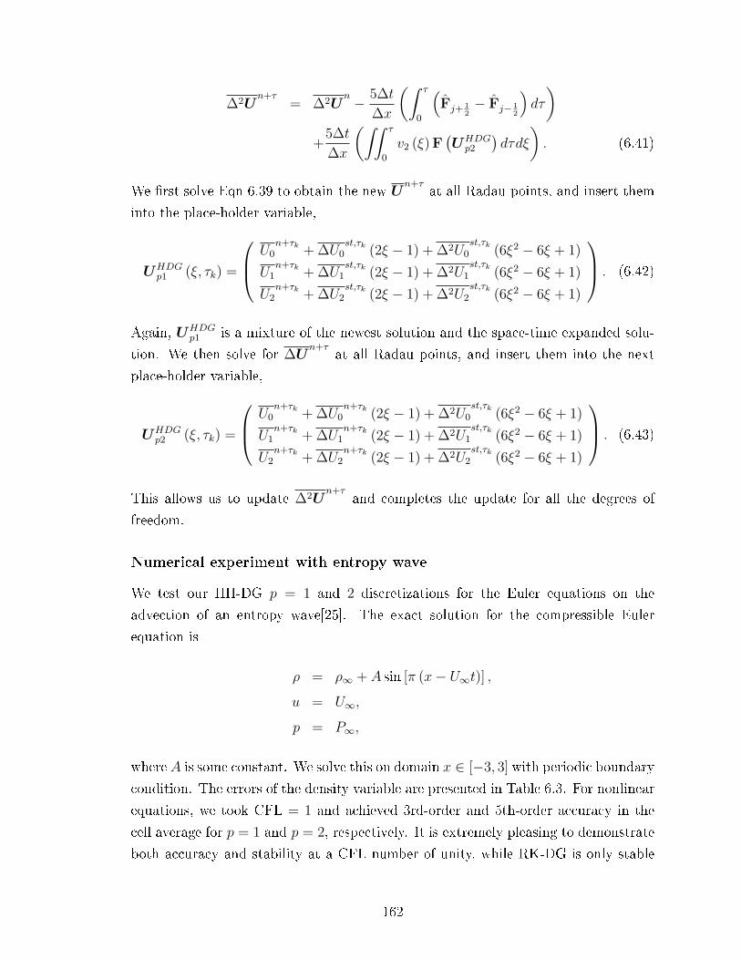
∆2Un+τ
= ∆2Un − 5∆t
∆x
(∫ τ
0
(Fj+ 1
2− Fj− 1
2
)dτ
)+
5∆t
∆x
(∫∫ τ
0
v2 (ξ) F(UHDGp2
)dτdξ
). (6.41)
We rst solve Eqn 6.39 to obtain the new Un+τ
at all Radau points, and insert them
into the place-holder variable,
UHDGp1 (ξ, τk) =
U0n+τk
+ ∆U0st,τk
(2ξ − 1) + ∆2U0st,τk
(6ξ2 − 6ξ + 1)
U1n+τk
+ ∆U1st,τk
(2ξ − 1) + ∆2U1st,τk
(6ξ2 − 6ξ + 1)
U2n+τk
+ ∆U2st,τk
(2ξ − 1) + ∆2U2st,τk
(6ξ2 − 6ξ + 1)
. (6.42)
Again, UHDGp1 is a mixture of the newest solution and the space-time expanded solu-
tion. We then solve for ∆Un+τ
at all Radau points, and insert them into the next
place-holder variable,
UHDGp2 (ξ, τk) =
U0n+τk
+ ∆U0n+τk
(2ξ − 1) + ∆2U0st,τk
(6ξ2 − 6ξ + 1)
U1n+τk
+ ∆U1n+τk
(2ξ − 1) + ∆2U1st,τk
(6ξ2 − 6ξ + 1)
U2n+τk
+ ∆U2n+τk
(2ξ − 1) + ∆2U2st,τk
(6ξ2 − 6ξ + 1)
. (6.43)
This allows us to update ∆2Un+τ
and completes the update for all the degrees of
freedom.
Numerical experiment with entropy wave
We test our HH-DG p = 1 and 2 discretizations for the Euler equations on the
advection of an entropy wave[25]. The exact solution for the compressible Euler
equation is
ρ = ρ∞ + A sin [π (x− U∞t)] ,u = U∞,
p = P∞,
where A is some constant. We solve this on domain x ∈ [−3, 3] with periodic boundary
condition. The errors of the density variable are presented in Table 6.3. For nonlinear
equations, we took CFL = 1 and achieved 3rd-order and 5th-order accuracy in the
cell average for p = 1 and p = 2, respectively. It is extremely pleasing to demonstrate
both accuracy and stability at a CFL number of unity, while RK-DG is only stable
162

with CFL = 0.4 and 0.27 for p = 1 and 2, respectively (see Section 3.4.1).
Nele DOF L2 ρerror Rate L24ρerror Rate
12 24 3.14× 10⁻¹ 2.57× 10⁻¹
24 48 1.54× 10⁻¹ 1.0 6.18× 10⁻² 2.048 96 2.60× 10⁻² 2.6 5.41× 10⁻³ 3.596 192 3.42× 10⁻³ 3.0 5.91× 10⁻⁴ 3.2192 384 4.31× 10⁻⁴ 3.0 5.05× 10⁻⁵ 3.6384 768 5.39× 10⁻⁵ 3.0 2.19× 10⁻⁵ 1.2
Nele DOF L2 ρerror Rate L24ρerror Rate L242ρerror Rate
12 24 8.53× 10⁻³ 8.49× 10⁻³ 3.32× 10⁻³
24 48 3.35× 10⁻⁴ 4.7 4.79× 10⁻⁵ 7.5 7.08× 10⁻⁵ 5.548 96 1.14× 10⁻⁵ 4.9 1.99× 10⁻⁵ 1.3 8.56× 10⁻⁶ 3.196 192 4.09× 10⁻⁷ 4.8 2.88× 10⁻⁶ 2.8 5.29× 10⁻⁷ 4.0192 384 1.60× 10⁻⁸ 4.7 3.77× 10⁻⁷ 3.0 1.03× 10⁻⁷ 2.4384 768 6.00× 10⁻¹⁰ 4.7 3.58× 10⁻⁸ 3.4 4.98× 10⁻⁸ 1.1
Table 6.3: Entropy wave case: order of accuracy for HH-DG p = 1 and 2, CFL = 1.0,tfinal = 50. A density sine-wave is advected over 50 periods, while velocityand total energy remain constant.
Numerical experiment with a single expansion wave
The previous experiment is really just a single advection equation for density; in
this experiment we take on a harder problem where all the conserved variables are
coupled. Consider a single expansion wave[25] centered in x ∈ [0, 1] with the following
solutions,
V (ξ) = (0.02) tanh (10 (x− 0.5− V t)) , (6.44)
u (x, t)
a∞= M∞ +
2
γ + 1
V (ξ)
a∞, (6.45)
ρ (x, t)
ρ∞=
[1 +
γ − 1
2
(u (ξ)
a∞−M∞
)] 2γ−1
, (6.46)
p (x, t)
p∞=
[1 +
γ − 1
2
(u (ξ)
a∞−M∞
)] 2γγ−1
, (6.47)
163
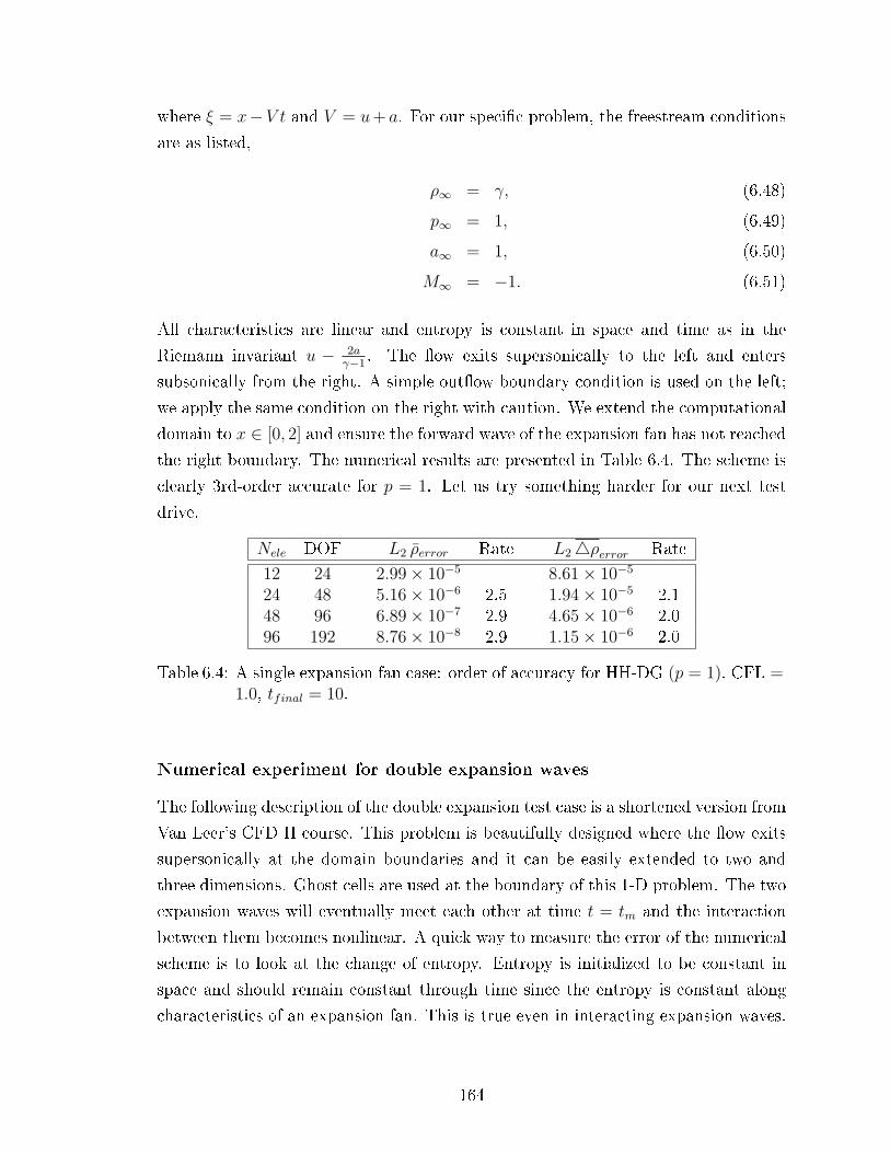
where ξ = x−V t and V = u+ a. For our specic problem, the freestream conditions
are as listed,
ρ∞ = γ, (6.48)
p∞ = 1, (6.49)
a∞ = 1, (6.50)
M∞ = −1. (6.51)
All characteristics are linear and entropy is constant in space and time as in the
Riemann invariant u − 2aγ−1
. The ow exits supersonically to the left and enters
subsonically from the right. A simple outow boundary condition is used on the left;
we apply the same condition on the right with caution. We extend the computational
domain to x ∈ [0, 2] and ensure the forward wave of the expansion fan has not reached
the right boundary. The numerical results are presented in Table 6.4. The scheme is
clearly 3rd-order accurate for p = 1. Let us try something harder for our next test
drive.
Nele DOF L2 ρerror Rate L24ρerror Rate
12 24 2.99× 10⁻⁵ 8.61× 10⁻⁵
24 48 5.16× 10⁻⁶ 2.5 1.94× 10⁻⁵ 2.148 96 6.89× 10⁻⁷ 2.9 4.65× 10⁻⁶ 2.096 192 8.76× 10⁻⁸ 2.9 1.15× 10⁻⁶ 2.0
Table 6.4: A single expansion fan case: order of accuracy for HH-DG (p = 1), CFL =1.0, tfinal = 10.
Numerical experiment for double expansion waves
The following description of the double expansion test case is a shortened version from
Van Leer's CFD II course. This problem is beautifully designed where the ow exits
supersonically at the domain boundaries and it can be easily extended to two and
three dimensions. Ghost cells are used at the boundary of this 1-D problem. The two
expansion waves will eventually meet each other at time t = tm and the interaction
between them becomes nonlinear. A quick way to measure the error of the numerical
scheme is to look at the change of entropy. Entropy is initialized to be constant in
space and should remain constant through time since the entropy is constant along
characteristics of an expansion fan. This is true even in interacting expansion waves.
164

Consider the following problem initialization on the the domain x ∈ [−3, 3],
u =
u∞,L x < −1.5
a∞
(M∞,L − u∞,L
2a∞tanh
(x+1
14−(x+1)2 + 1
))−1.5 ≤ x ≤ −0.5
0 −0.5 < x < 0.5
a∞
(M∞,R +
u∞,R2a∞
tanh(
x−114−(x+1)2 − 1
))0.5 ≤ x ≤ 1.5
u∞,R x > 1.5
, (6.52)
with the following conditions in the freestreams on the left and right side,
u∞,L = 2/√γ, (6.53)
u∞,R = −2/√γ, (6.54)
M∞,L = −2, (6.55)
M∞,R = 2, (6.56)
a∞ = 1/√γ, (6.57)
with γ = 1.4. The equations for density and pressure come from the previous test
case. The change in entropy is also dened to be the error of the numerical scheme,
S = ∆s = log
((ptfinalργtfinal
)/
(pt0ργt0
)), (6.58)
where t0 = 0 and tfinal = 2. The results for p = 1 and 2 are shown in Table 6.5.
It appears for this highly nonlinear problem that the results on the coarsest grids
are not ne enough to capture the complex interaction of the two expansion waves.
The order of accuracy is better revealed on the ner grids where the p = 1 scheme is
3rd-order accurate, and roughly 4th-order accurate for p = 2. The latter accuracy is
disappointing as we expected 5th-order acuracy (2p + 1). Moreover, we have notice
that the L∞ error norm (not shown) is one order lower than L2; this is indeed puzzling
and will be left for future investigation.
6.2.3 Summary of HH-DG for advection
HH-DG is a space-time DG scheme that mimics the exact shift operator. The scheme
is blessed with the good spatial accuracy of a typical DG scheme; it is also the rst
scheme to achieve CFL = 1 for all p. The secret comes in the careful evaluation
of both surface and volume integrals. We demonstrated the volume integral must
165

Nele DOF L2 Serror Rate L2 ∆Serror Rate
12 24 2.41× 10⁻² 8.53× 10⁻²
24 48 4.25× 10⁻³ 2.5 1.44× 10⁻² 2.548 96 3.02× 10⁻⁴ 3.8 1.52× 10⁻³ 3.296 192 3.85× 10⁻⁵ 2.9 1.99× 10⁻⁴ 2.9192 384 5.00× 10⁻⁶ 2.9 2.92× 10⁻⁵ 2.7384 768 6.96× 10⁻⁷ 2.8 4.91× 10⁻⁶ 2.5
Nele DOF L2 Serror Rate L2 ∆Serror Rate L2 ∆2Serror Rate
12 24 2.46× 10⁻² 3.46× 10⁻² 5.96× 10⁻²
24 48 1.61× 10⁻³ 3.9 1.85× 10⁻³ 4.2 5.05× 10⁻³ 3.548 96 4.01× 10⁻⁴ 2.0 3.14× 10⁻⁴ 2.5 3.21× 10⁻⁴ 3.996 192 3.36× 10⁻⁵ 3.5 2.68× 10⁻⁵ 3.5 2.07× 10⁻⁵ 3.9192 384 1.61× 10⁻⁶ 4.3 1.55× 10⁻⁶ 4.1 1.29× 10⁻⁶ 4.0384 768 8.36× 10⁻⁸ 4.2 1.15× 10⁻⁷ 3.7 8.33× 10⁻⁸ 3.9
Table 6.5: Double expansion fans case: order of accuracy for HH-DG p = 1 and 2,CFL = 1.0, tfinal = 2. Two expansion waves expand and interact at thecenter of the domain. The error is given by the change of entropy whichis supposed to be zero.
include wave interaction in order to achieve good accuracy and stability. Numerical
results for linear advection conrm the excellent stability and accuracy of HH-DG
and the use of a local linear RK procedure to replace the CK procedure. As for the
results for Euler equations, HH-DG works very well for p = 1 (which is expected since
it is identical to Huynh's moment scheme); however, much work is ahead to ensure
the p = 2 version works as well as its linear counterpart.
6.3 Space-time discontinuous Galerkin for diusion
The HH-DG advection operator demonstrates remarkable robustness and high-order
accuracy. We wish to repeat that success in the HH-DG diusion operator; precisely,
we want to combine HH-DG with RDG to form the Hancock-Huynh recovery-based
DG (HH-RDG) scheme. Unlike the previous section where we have an exact op-
erator to replicate, our design objective is to obtain a diusion scheme with the
highest possible Von Neumann number (VNN). We establish a few high-order dif-
fusion schemes based on the classical nite-dierence framework, and a version of
nite dierence with subgrid information. These schemes will provide a basis for
comparison and insight into designing space-time diusion schemes.
166
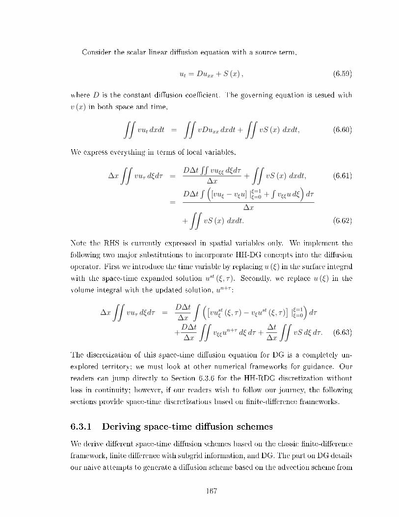
Consider the scalar linear diusion equation with a source term,
ut = Duxx + S (x) , (6.59)
where D is the constant diusion coecient. The governing equation is tested with
v (x) in both space and time,∫∫vut dxdt =
∫∫vDuxx dxdt+
∫∫vS (x) dxdt, (6.60)
We express everything in terms of local variables,
∆x
∫∫vuτ dξdτ =
D∆t∫∫
vuξξ dξdτ
∆x+
∫∫vS (x) dxdt, (6.61)
=D∆t
∫ ([vuξ − vξu] |ξ=1
ξ=0 +∫vξξu dξ
)dτ
∆x
+
∫∫vS (x) dxdt. (6.62)
Note the RHS is currently expressed in spatial variables only. We implement the
following two major substitutions to incorporate HH-DG concepts into the diusion
operator. First we introduce the time variable by replacing u (ξ) in the surface integral
with the space-time expanded solution ust (ξ, τ). Secondly, we replace u (ξ) in the
volume integral with the updated solution, un+τ :
∆x
∫∫vuτ dξdτ =
D∆t
∆x
∫ ([vustξ (ξ, τ)− vξust (ξ, τ)
]|ξ=1ξ=0
)dτ
+D∆t
∆x
∫∫vξξu
n+τ dξ dτ +∆t
∆x
∫∫vS dξ dτ. (6.63)
The discretization of this space-time diusion equation for DG is a completely un-
explored territory; we must look at other numerical frameworks for guidance. Our
readers can jump directly to Section 6.3.6 for the HH-RDG discretization without
loss in continuity; however, if our readers wish to follow our journey, the following
sections provide space-time discretizations based on nite-dierence frameworks.
6.3.1 Deriving space-time diusion schemes
We derive dierent space-time diusion schemes based on the classic nite-dierence
framework, nite dierence with subgrid information, and DG. The part on DG details
our naive attempts to generate a diusion scheme based on the advection scheme from
167
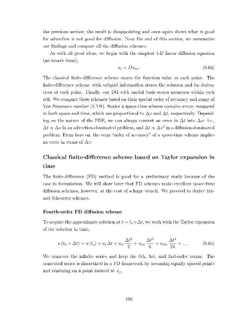
the previous section; the result is disappointing and once again shows what is good
for advection is not good for diusion. Near the end of this section, we summarize
our ndings and compare all the diusion schemes.
As with all great ideas, we begin with the simplest 1-D linear diusion equation
(no source term),
ut = Duxx. (6.64)
The classical nite-dierence scheme stores the function value at each point. The
nite-dierence scheme with subgrid information stores the solution and its deriva-
tives at each point. Finally, our DG with modal basis stores moments within each
cell. We compare these schemes based on their spatial order of accuracy and range of
Von Neumann number (VNN). Notice a space-time scheme contains errors measured
in both space and time, which are proportional to ∆x and ∆t, respectively. Depend-
ing on the nature of the PDE, we can always convert an error in ∆t into ∆x: i.e.,
∆t ∝ ∆x in an advection-dominated problem, and ∆t ∝ ∆x2 in a diusion-dominated
problem. From here on, the term order of accuracy of a space-time scheme implies
an error in terms of ∆x.
Classical nite-dierence scheme based on Taylor expansion in
time
The nite-dierence (FD) method is good for a preliminary study because of the
ease in formulation. We will show later that FD schemes make excellent space-time
diusion schemes, however, at the cost of a large stencil. We proceed to derive 4th-
and 6th-order schemes.
Fourth-order FD diusion scheme
To acquire the approximate solution at t = to+∆t, we work with the Taylor expansion
of the solution in time,
u (t0 + ∆t) = u (to) + ut ∆t+ utt∆t2
2+ uttt
∆t3
6+ utttt
∆t4
24+ . . . (6.65)
We truncate the innite series and keep the 0th, 1st, and 2nd-order terms. The
truncated series is discretized in a FD framework by assuming equally spaced points
and centering on a point located at xj,
168

uj (t0 + ∆t) = uj (to) + ut,j ∆t+ utt,j∆t2
2. (6.66)
The two temporal derivatives are transformed into spatial derivatives via the Cauchy-
Kovalevskaya (CK) procedure and then approximated with central nite-dierence
operators; our rst pass at this gives
ut,j = Duxx,j ≈ D∆2uj∆x2
= Duj+1 − 2uj + uj−1
∆x2, (6.67)
utt,j = D2uxxxx,j ≈ D2 ∆4uj∆x4
= D2 ∆2 (∆2uj)
∆x4= D2uj+2 − 4uj+1 + 6uj − 4uj−1 + uj−2
∆x4.
(6.68)
Notice the approximately equal signs are used since the nite-dierence operators used
here contain numerical errors. The crudeness of the approximation is quantied by
Taylor expanding the solution in space,
uj±l = u (xj ± l∆x) = uj±ux,j l∆x+uxx,j(l∆x)2
2±uxxx,j
(l∆x)3
6+uxxxx,j
(l∆x)4
24+. . . ,
(6.69)
where l is an integer. We rst look at the error in the second derivative. Inserting
the Taylor expansion into Eqn 6.67 yields
∆2uj∆x2
= uxx,j + uxxxx,j∆x2
12+ uxxxxxx,j
∆x4
360+O
(∆x6
). (6.70)
This 2nd-order dierence operator approximates the real second derivative uxx with
an error of O (∆x2). Since this term gets multiplied by ∆t in Eqn 6.66, the nal
error becomes O (∆x4) for a diusion-dominated problem. We seek to improve upon
the approximation of uxx by adding a correction term to Eqn 6.70 to remove the
2nd-order error,
uxx,j ≈∆2uj∆x2
− uxxxx,j∆x2
12, (6.71)
hence our slightly rened approximation of uxx contains an error of O (∆x4). We look
at the error in the fourth derivative by inserting the Taylor expansion into Eqn 6.68,
∆4uj∆x4
= uxxxx,j + u(6),j∆x2
6+ u(8),j
∆x4
80+O
(∆x6
), (6.72)
The O (∆x2) error is acceptable since this term is multiplied with ∆t2 ∝ ∆x4, result-
ing in a nal error of O (∆x6). Inserting Eqns 6.68 and 6.71 into Eqn 6.90 results in
169

a scheme that is 4th-order in space,
uj (t0 + ∆t) = uj (to) +D∆t
(∆2uj∆x2
− 1
12
∆4uj∆x2
)+D2∆t2
2∆x4∆4uj,
= uj (to) + r∆2uj +
(r2
2− r
12
)∆4uj, (6.73)
where r is the shorthand notation of the Von Neumann number,
r =D∆t
∆x2. (6.74)
We replace central-dierence operators with Fourier mode
uj = eiβj, (6.75)
and acquire an amplication factor of
g (r, β) = 1 + 2r (cosβ − 1) + 4
(r2
2− r
12
)(cosβ − 1)2 . (6.76)
Figure 6.6 shows the amplication factor for dierent values of r. The line with r = 23
represents the highest possible VNN without inducing instability.
0 1 2 3 4 5 60.2
0.3
0.4
0.5
0.6
0.7
0.8
0.9
1
r = 0.10
r = 0.45
r = 0.66
β
g
Figure 6.6: Amplication factor of the 4th-order diusion scheme using central dif-ferencing. A maximum of r = 0.66 is achieved with regard to stability.
170

6th-order FD diusion scheme
We quickly generate a 6th-order FD diusion scheme without detailing too much of
the mathematics. The 6th-order central-dierence operator is
∆6uj∆x6
=uj+3 − 6uj+2 + 15uj+1 − 20uj + 15uj−1 − 6uj−2 + uj−3
∆x6. (6.77)
Inserting the Taylor expansion (Eqn 6.69) results in
∆6uj∆x6
= u(6),j + u(8),j∆x2
8+O
(∆x4
); (6.78)
the 2nd-order error is ne since it is multiplied by ∆t3 ∝ ∆x6, resulting in an error of
O (∆x8). We use 6th-order central-dierence operator to improve upon the 4th-order
operator in Eqn 6.68,
uxxxx,j ≈∆4uj∆x4
− u(6),j∆x2
6. (6.79)
We then use the 6th derivative together with the improved 4th derivative to correct
the errors in the 2nd-order central dierence operator,
uxx,j ≈∆2uj∆x2
− uxxxx,j∆x2
12+ u(6),j
∆x4
90. (6.80)
Inserting Eqns 6.78-6.80 into Eqn 6.65 results in the following 6th-order FD scheme,
uj (t0 + ∆t) = uj (to) +D∆t
(∆2uj∆x2
− 1
12
∆4uj∆x2
+1
90
∆6uj∆x2
)+D2∆t2
2
(∆4uj∆x4
− 1
6
∆6uj∆x4
)+D3∆t3
6
(∆6uj∆x6
), (6.81)
with the following amplication factor,
g (r, β) = 1 + 2r (cosβ − 1) + 4
(r2
2− r
12
)(cosβ − 1)2
+8
(r3
6− r2
12+
r
90
)(cosβ − 1)3 . (6.82)
We present a plot of the amplication factor in Figure 6.7. The scheme is stable for
VNN up to 0.8413.
171

r = 0.84
r = 0.66
r = 0.50
0 1 2 3 4 5 6
-1.0
-0.5
0.0
0.5
1.0
Β
g
Figure 6.7: Amplication factor of the 6th-order diusion scheme using central dif-ferencing. A maximum of r = 0.84 is achieved.
Summary of FD ndings
The classical FD framework generates space-time diusion schemes with very high
VNN's. The 4th-order scheme with a 5-point stencil obtains a maximum VNN of
0.66, while the 6th-order scheme with a 7-point stencil obtains a maximum VNN of
0.84. Perhaps the most surprising nding in this exercise is that a growing stencil
for diusion increases the VNN; this is contrary to advection where a growing stencil
centered around the update point (as in RK) decreases the CFL number. We believe
a growing stencil mimics the innite propagation speed of the characteristics in a
diusion equation; in contrast, a growing stencil for advection brings in additional
information from downwind, which is destabilizing. However, a growing stencil greatly
increases the complexity of the code for unstructured grids and makes boundary
treatment a nightmare. We proceed to look at FD schemes with subgrid information
to see what we can achieve with a compact stencil.
Finite-dierence scheme with subgrid information based on Tay-
lor expansion in time
We delve into two FD schemes with subgrid information. Considering equally spaced
points, we consider a p = 1 scheme with the solution value and its rst derivative
stored at each point, and then a p = 2 scheme with the solution value and its rst
and second derivatives stored at each point.
172

FD with p = 1 subgrid information
We consider an FD scheme with p = 1 subgrid information; this allows us to store the
solution value u and its rst derivative ux at each point. The manner of analysis is
the same as the previous section applied to a system instead. Consider the 2nd-order
Taylor expansion of the solution and its derivative in time,
uj (t0 + ∆t) = uj (to) + ut,j ∆t+ utt,j∆t2
2,
ux,j (t0 + ∆t) = ux,j (to) + uxt,j ∆t+ uxtt,j∆t2
2. (6.83)
Our strategy is to t a 5th-order polynomial through the three points and obtain its
derivatives via a CK procedure,
ut = Duxx ≈2D (uj+1 − 2uj + uj−1)
∆x2− D (ux,j+1 − ux,j−1)
2∆x,
uxt = Duxxx ≈15D (uj+1 − uj−1)
2∆x3− 3D (ux,j+1 + 8ux,j + ux,j−1)
2∆x2,
utt = D2uxxxx ≈ −12D2 (uj+1 − 2uj + uj−1)
∆x4+
6D2 (ux,j+1 − ux,j−1)
∆x3,
uxtt = D2uxxxxx ≈ −90D2 (uj+1 − uj−1)
∆x5
−30D2 (ux,j+1 + 4ux,j + ux,j−1)
∆x4. (6.84)
Inserting Eqn 6.69 and the Taylor expansion of ux,j below,
ux,j±1 = ux (xj ±∆x) = ux,j±uxx,j ∆x+uxxx,j∆x2
2±uxxxx,j
∆x3
6+uxxxxx,j
∆x4
24+. . . ,
(6.85)
gives us the error associated with each approximation of the derivatives,
E (uxx,j) = −∆x4
360uxxxxxx,j +O
(∆x6
),
E (uxxx,j) = −∆x4
240uxxxxxxx,j +O
(∆x6
),
E (uxxxx,j) = +∆x2
15uxxxxxx,j +O
(∆x4
),
E (uxxxxx,j) = +∆x4
12uxxxxxxx,j +O
(∆x4
). (6.86)
This means the RHS of Eqn 6.83 contains spatial errors of O (∆x6); however, since
Eqn 6.83 is only 2nd-order in time, the resulting scheme is 4th-order accurate for
173

time-dependent problems, and 6th-order accurate for steady-state problems. The
system can be expressed in terms of Fourier mode β,(un+1
un+1x
)j
=
(un
unx
)j
+M (r, β)
(un
unx
)j
, (6.87)
where M is a 2× 2 matrix,
M =
[−4r + 12r2 + 4r cos (β)− 12r2 cos (β) −i r∆x sin (β) + 6 i r2 ∆x sin (β)
15 i r sin(β)∆x
− 90 i r2 sin(β)∆x
−12r + 60r2 − 3r cos (β) + 30r2 cos (β)
].
(6.88)
Let λ1,2 be the two eigenvalues of M , then the amplication factors are
g1,2 = 1 + λ1,2 (r, β) . (6.89)
Figure 6.8 shows the two amplication factors for various values of r. Notice this
4th-order scheme using a compact stencil with subgrid information has a maximum
r of 16.
0 2 4 60.3
0.4
0.5
0.6
0.7
0.8
0.9
1
r = 112
β
g
0 2 4 60.3
0.4
0.5
0.6
0.7
0.8
0.9
1
r = 16
β
g
Figure 6.8: The two amplication factors associated with a nite-dierence schemewith p = 1 subgrid information. The resulting scheme is 4th-order accu-rate in time. Notice for r = 1
12, the two amplication factors are distinct,
while for r = 16, the two amplication factors coincide with each other.
FD with p = 2 subgrid information
We derive a 6th-order FD scheme for diusion with piecewise-quadratic (p = 2)
subgrid information; the variables u, ux, and uxx stored at each point. Consider the
174

3rd-order Taylor expansion of the three variables in time,
uj (t0 + ∆t) = uj (to) + ut,j ∆t+ utt,j∆t2
2+ uttt,j
∆t3
6,
ux,j (t0 + ∆t) = ux,j (to) + uxt,j ∆t+ uxtt,j∆t2
2+ uxttt,j
∆t3
6,
uxx,j (t0 + ∆t) = uxx,j (to) + uxxt,j ∆t+ uxxtt,j∆t2
2+ uxxttt,j
∆t3
6. (6.90)
This time we t a 8th-order polynomial through the three points and obtain its
derivatives via a CK procedure,
u(3),j ≈ − 3
8∆x3
(35 (uj−1 − uj+1) + 11∆x
(ux,j+1 +
48
11ux,j + ux,j−1
))− 3
8∆x3
(∆x2 (uxx,j−1 − uxx,j+1)
), (6.91)
u(4),j ≈ − 3
2∆x4(48 (−uj−1 + 2uj − uj+1) + 13∆x (ux,j+1 − ux,j−1))
− 3
2∆x4
(∆x2 (−uxx,j−1 + 24uxx,j − uxx,j+1)
), (6.92)
u(5),j ≈ − 15
∆x5
(−21 (uj−1 + uj+1) + 9∆x
(−ux,j+1 −
24
9ux,j − ux,j−1
))− 15
∆x5
(∆x2 (uxx,j−1 − uxx,j+1)
), (6.93)
u(6),j ≈ − 90
∆x6(32 (uj−1 − 2uj + uj+1) + 11∆x (−ux,j+1 + ux,j−1))
− 90
∆x6
(∆x2 (uxx,j−1 − 12uxx,j + uxx,j+1)
), (6.94)
u(7),j ≈ − 315
∆x7(15 (uj−1 − uj+1) + ∆x (7ux,j+1 + 16ux,j + 7ux,j−1))
− 315
∆x7
(∆x2 (−uxx,j−1 + uxx,j+1)
), (6.95)
u(8),j ≈ −2520
∆x8(24 (−uj−1 + 2uj − uj+1) + ∆x (9ux,j+1 − 9ux,j−1))
−2520
∆x8
(∆x2 (−uxx,j−1 + 8uxx,j − uxx,j+1)
), (6.96)
175

Inserting the Taylor expansion of uj into Eqn 6.69, ux,j into Eqn 6.85, together with
the Taylor expansion of uxx,j below,
uxx,j±1 = uxx (xj ±∆x) = uxx,j±uxxx,j ∆x+uxxxx,j∆x2
2±uxxxxx,j
∆x3
6+uxxxxxx,j
∆x4
24+. . . ,
(6.97)
gives us the error associated with each approximation of the derivative,
E (uxxx,j) = − ∆x6
17920ux(5),j +O
(∆x8
),
E (uxxxx,j) = +∆x6
13440ux(6),j +O
(∆x8
),
E(ux(5),j
)= +
∆x4
1344ux(7),j +O
(∆x6
),
E(ux(6),j
)= −∆x4
224ux(8),j +O
(∆x6
),
E(ux(7),j
)= +
∆x2
64ux(9),j +O
(∆x4
),
E(ux(8),j
)= +
∆x2
8ux(10),j +O
(∆x4
). (6.98)
The resulting method is 8th-order accurate in space, and 6th-order accurate in time.
We rewrite the update equations in matrix form, un+1
un+1x
un+1xx
j
=
un
unx
unxx
j
+M (r, β)
un
unx
unxx
j
, (6.99)
whereM is a 3×3 matrices. The matrix and its eigenvalues are omitted here; only the
amplication factors are shown in Figure 6.9. This scheme is stable up to r = 0.124;
however, the eigenvalues only remain real up to r = 0.0529.
Summary of FD with subgrid information ndings
FD schemes with subgrid information produce high-resolution spatial discretizations;
e.g., p = 1 is 6th-order accurate in space and p = 2 is 8th-order accurate in space.
However, these schemes are only 4th- and 6th-order accurate in time. In addition,
their VNN is much lower than that of the classical FD schemes. We clearly see
that using a compact stencil has an adverse eect on the VNN; the above schemes
represent the best one can do with a compact stencil using subgrid information.
176

0 1 2 3 4 5 6
0.2
0.4
0.6
0.8
1.0
Β
g
0 1 2 3 4 5 6-1.0
-0.5
0.0
0.5
1.0
Β
g
Figure 6.9: The three amplication factors associated with the FD scheme with p = 2subgrid information is shown for r = 0.0529 (left) and r = 0.124 (right).The eigenvalues are real up to r = 0.0529. The eigenvalues become com-plex for r ≥ 0.0529 and the amplication factors remain under unity uptill r = 0.124.
DG schemes based on Hancock's observation: The rise of HH-
RDG
The concepts in the FD scheme with subgrid information can be easily ported into the
DG framework via a change of basis from nodal (strong interpolation) to modal (weak
interpolation). However, this time around we shall derive a DG diusion scheme using
Hancock's observation instead of Taylor expansions in time.
We wish to replicate the HH-DG advection operator for diusion; unfortunately,
what works for the gander does not work for the goose. If we naively replicate our
procedure for advection, the resulting diusion scheme will be poor in accuracy and
low in VNN; we will show this in three of our naive attempts below. In addition,
the diusion equation exhibits a dierent scaling of time and space, which ultimately
aects the conversion of temporal to spatial derivatives.
Let us go through a little thought experiment and imagine the Cauchy-Kovalevaskaya
(CK) procedure as a black box that puts in spatial derivatives and puts out temporal
derivatives. For advection of the form ut = ux, the conversion rate is one-to-one.
In mathematical terminology, it means each spatial derivative of order k results in
a temporal derivative of the same order. Consider the piecewise-linear solution in
space with u and ux as variables. The CK procedure relates ut to ux, hence the set
of u, ux, ut forms a complete p = 1 space-time basis.
When dealing with diusion, the CK procedure does not work in our favor. With
diusion of the form, ut = uxx, the conversion rate becomes two-to-one. This means it
takes two spatial derivatives to get one temporal derivative. With the same piecewise-
177

linear solution in space with u and ux as variables, the CK procedure fails to yield
ut because uxx is not available. If one naively use the LL-RK (numerical version of
CK), the order of accuracy of the scheme is at most 2nd-order. This simple thought
experiment demonstrates that the CK procedures for advection and diusion require
completely dierent treatments. The x is simple; the CK procedure for the diusion
operator simply requires more information in the spatial direction than its advec-
tion counterpart. Next, we demonstrate numerically the three naive and one smart
attempts to incorporate Hancock's observation into DG diusion.
Naive scheme I: LL-RK applied on p = 1 solution, RDG (p = 1) at the
Radau points
In the rst of the series of naive attempts, we apply the LL-RK procedure on the
piecewise-linear solution, and then apply spatial RDG to recover cubic polynomials
at the two Radau time levels . We solve the steady-state linear diusion equation
with a source term,
ut = uxx + 4π2sin (2πx) , x ∈ [0 1] . (6.100)
Though one might question the use of a steady-state problem for a space-time scheme,
it turns out this simple problem is good enough to reveal stability limit and spatial
accuracy of the scheme. If the scheme cannot even achieve a good order of accuracy
in a steady-state problem, then there is no further need to test the scheme on a
time-accurate problem. The procedure is as follows: we sweep through all cells with
LL-RK to obtain u and ux at all Radau points. We then sweep through all interfaces
with RDG to obtain the recovered function at all Radau points. The steady-state
numerical results are provided in Table 6.6. This method fails to achieve 3rd-order
accuracy and obtains a maximum VNN of 18. Our rst attempt falls short of the
desired 4th-order of accuracy, and also fails to reach a modest goal of r = 16. With
a p = 1 solution, there is simply not enough spatial information per cell to obtain
a 1st-order time derivative. This observation leads us directly to our next naive
attempt.
178
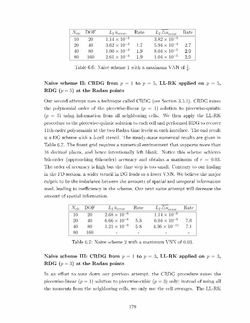
Nele DOF L2 uerror Rate L24uerror Rate
10 20 1.14× 10⁻² 3.82× 10⁻³
20 40 3.62× 10⁻³ 1.7 5.94× 10⁻⁴ 2.740 80 1.00× 10⁻³ 1.9 8.04× 10⁻⁵ 2.980 160 2.61× 10⁻⁴ 1.9 1.04× 10⁻⁵ 2.9
Table 6.6: Naive scheme 1 with a maximum VNN of 18.
Naive scheme II: CRDG from p = 1 to p = 5, LL-RK applied on p = 5,
RDG (p = 5) at the Radau points
Our second attempt uses a technique called CRDG (see Section 3.5.1). CRDG raises
the polynomial order of the piecewise-linear (p = 1) solution to piecewise-quintic
(p = 5) using information from all neighboring cells. We then apply the LL-RK
procedure to the piecewise-quintic solution to each cell and performed RDG to recover
11th-order polynomials at the two Radau time levels at each interface. The end result
is a DG scheme with a 5-cell stencil. The steady-state numerical results are given in
Table 6.7. The nest grid requires a numerical environment that supports more than
16 decimal places, and hence intentionally left blank. Notice this scheme achieves
5th-order (approaching 6th-order) accuracy and obtains a maximum of r = 0.03.
The order of accuracy is high but the time step is too small. Contrary to our nding
in the FD section, a wider stencil in DG leads to a lower VNN. We believe the major
culprit to be the imbalance between the amounts of spatial and temporal information
used, leading to ineciency in the scheme. Our next naive attempt will decrease the
amount of spatial information.
Nele DOF L2 uerror Rate L24uerror Rate
10 20 2.68× 10⁻⁶ 1.14× 10⁻⁶
20 40 6.66× 10⁻⁸ 5.3 6.04× 10⁻⁹ 7.640 80 1.21× 10⁻⁹ 5.8 4.36× 10⁻¹¹ 7.180 160 - - - -
Table 6.7: Naive scheme 2 with a maximum VNN of 0.03.
Naive scheme III: CRDG from p = 1 to p = 3, LL-RK applied on p = 3,
RDG (p = 3) at the Radau points
In an eort to tone down our previous attempt, the CRDG procedure raises the
piecewise-linear (p = 1) solution to piecewise-cubic (p = 3) only; instead of using all
the moments from the neighboring cells, we only use the cell averages. The LL-RK
179

procedure is applied to the piecewise-cubic solution and then RDG recovers a 7th-
order polynomials at the two Radau points. The numerical results are presented in
Table 6.8. The scheme approaches the 4th order of accuracy and the maximum VNN
is 0.04, representing a mere 30% improvement over the previous case. At this point,
it becomes apparent that we need to do something drastically dierent to increase
the stability limit.
Nele DOF L2 uerror Rate L24uerror Rate
10 20 2.28× 10⁻⁴ 6.78× 10⁻⁵
20 40 2.74× 10⁻⁵ 3.1 1.63× 10⁻⁶ 5.440 80 2.14× 10⁻⁶ 3.7 5.03× 10⁻⁸ 5.080 160 1.47× 10⁻⁷ 3.9 1.62× 10⁻⁹ 5.0
Table 6.8: Naive scheme 3 with maximum VNN of 0.04.
Summary of the three naive attempts
We make two important observations from the three naive attempts. First, a CK (or
LL-RK) procedure applied to a piecewise-linear solution is insucient for obtaining a
rst-order temporal derivative. Second, naive schemes II and III attempt to remedy
the rst problem by converting the original p = 1 solution into a high-order solution,
but the result is even worse than for the rst naive scheme in terms of VNN. It is clear
using the same approach as for the HH-DG advection operator is leading nowhere,
and a drastically new strategy is needed. The next section humbly presents a scheme
resolving these two issues.
Smart attempt IV (HH-RDG): LL-RK applied on RDG (p = 1)
We seek a completely dierent approach by applying the CK (or LL-RK) procedure
on the recovered function. Instead of acquiring a local evolution of the solution, we
acquire the local evolution of the recovered function! This scheme only applies the
recovery procedure once at τ = 0 instead of multiple times at dierent Radau points.
Since only the function value and the rst derivative are required at the interface, the
CK procedure is applied on the recovered function f in the dierential form. This is
much cheaper compared to the integral form because Gaussian integration is avoided.
The end result is a space-time recovered function, f st, that is a function of time.
Starting with a piecewise-linear solution at τ = 0 for all elements Ωj, we recover
an unique cubic recovery function fj+ 12between elements Ωj and Ωj+1. Note we are
using the same Legendre polynomials from Chapter 3. The recovered function fj+ 12
180

contains 4 unique coecients bk,j+ 12,
fj+ 12
= b0,j+ 12
+ b1,j+ 12r + b2,j+ 1
2r2 + b3,j+ 1
2r3, r ∈ [−1
2
1
2], (6.101)
where r now represents the coordinate normal to the interface; as in Section 3.1. The
interface lies on r = 0. The local coordinate r is conned to [−12
12], and is related to
x ∈ [−∆x ∆x] through r = x2∆x
, hence ∂r∂x
= 12∆x
. We enforce the recovered function
fj+ 12to satisfy the original PDE, and 3 derivatives of the PDE,
ft = D fxx + S (x) ,
fxt = D fxxx +∂
∂xS (x) ,
fxxt = D fxxxx +∂2
∂x2S (x) ,
fxxxt = D fxxxxx +∂3
∂x3S (x) . (6.102)
Notice the subscript j+ 12is dropped. We obtain the residual update form by inserting
Eqn 6.101 with r = 0 into Eqn 6.102:f
fx
fxx
fxxxx
t
=
b0
b1
(∂r∂x
)2b2
(∂r∂x
)2
6b3
(∂r∂x
)3
t
=
Dfrr/ (2∆x)2 + (2π)2 sin (2πx)
Dfrrr/ (2∆x)3 + (2π)3 cos (2πx)
Dfrrrr/ (2∆x)4 − (2π)4 sin (2πx)
Dfrrrrr/ (2∆x)5 − (2π)5 cos (2πx)
,
=
D (2b2) / (2∆x)2 + (2π)2 sin (2πx)
D (6b3) / (2∆x)3 + (2π)3 cos (2πx)
− (2π)4 sin (2πx)
− (2π)5 cos (2πx)
.
The RHS expressions are input as Res to the LL-RK update in Eqn 6.17. We
advance this system with LL-RK to the Radau points; we have obtained f st (τ) at
181

the Radau points only. We replace ust in the surface integral of Eqn 6.63 with f st,
∆x
∫∫vuτ dξdτ =
D∆t
∆x
∫ ([vf stξ (τ)− vξf st (τ)
]|ξ=1ξ=0
)dτ
+D∆t
∆x
∫∫vξξu
n+τ dξ dτ + ∆x∆t
∫∫vS dξ dτ. (6.103)
Note the volume integral for p = 1 is zero. The numerical results for smart scheme IV
are presented in Table 6.9. The scheme clearly demonstrates 4th-order of accuracy
and obtains a maximum VNN of 16, representing a healthy combination of accuracy
and speed. The next logical step is to repeat the same feat for piecewise-quadratic
DG (p = 2).
Nele DOF L2 uerror Rate L24uerror Rate
10 20 1.67× 10⁻⁴ 1.11× 10⁻⁴
20 40 1.15× 10⁻⁵ 3.9 3.43× 10⁻⁶ 5.040 80 7.58× 10⁻⁷ 3.9 1.04× 10⁻⁷ 5.080 160 4.86× 10⁻⁸ 4.0 3.04× 10⁻⁹ 5.1160 320 3.05× 10⁻⁹ 4.0 7.49× 10⁻¹¹ 5.3320 640 1.84× 10⁻¹⁰ 4.1 1.76× 10⁻¹² 5.4
Table 6.9: Smart scheme IV with a maximum VNN of 16. The smart scheme IV will
soon be named the HH-RDG scheme.
Smart attempt IV (HH-RDG): LL-RK applied on RDG (p = 2) with cor-
rect volume integral
For p ≥ 2, the volume integral enters into the update equation of the 2nd gradient
and hence must be treated carefully. We follow the same technique as applied to the
volume integral in the advection operator, which is to inltrate the volume integral
with information from neighboring elements. Starting with a piecewise-quadratic
solution at τ = 0 for all elements Ωj, we recover an unique quintic recovered function
fj+ 12between elements Ωj and Ωj+1. The recovered function fj+ 1
2contains 6 unique
coecients bk,j+ 12,
fj+ 12
= b0,j+ 12+b1,j+ 1
2r+b2,j+ 1
2r2+b3,j+ 1
2r3+b4,j+ 1
2r4+b5,j+ 1
2r5, r ∈ [−1
2
1
2], (6.104)
182
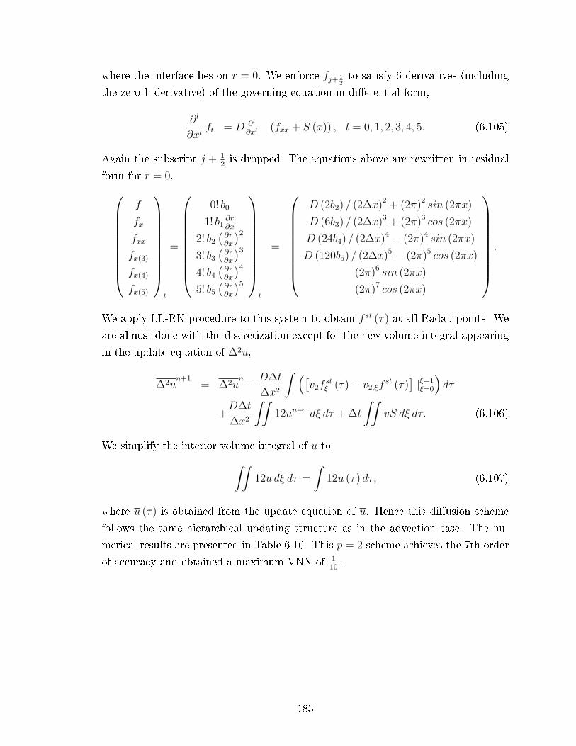
where the interface lies on r = 0. We enforce fj+ 12to satisfy 6 derivatives (including
the zeroth derivative) of the governing equation in dierential form,
∂l
∂xlft = D ∂l
∂xl(fxx + S (x)) , l = 0, 1, 2, 3, 4, 5. (6.105)
Again the subscript j + 12is dropped. The equations above are rewritten in residual
form for r = 0,
f
fx
fxx
fx(3)
fx(4)
fx(5)
t
=
0! b0
1! b1∂r∂x
2! b2
(∂r∂x
)2
3! b3
(∂r∂x
)3
4! b4
(∂r∂x
)4
5! b5
(∂r∂x
)5
t
=
D (2b2) / (2∆x)2 + (2π)2 sin (2πx)
D (6b3) / (2∆x)3 + (2π)3 cos (2πx)
D (24b4) / (2∆x)4 − (2π)4 sin (2πx)
D (120b5) / (2∆x)5 − (2π)5 cos (2πx)
(2π)6 sin (2πx)
(2π)7 cos (2πx)
.
We apply LL-RK procedure to this system to obtain f st (τ) at all Radau points. We
are almost done with the discretization except for the new volume integral appearing
in the update equation of ∆2u,
∆2un+1
= ∆2un − D∆t
∆x2
∫ ([v2f
stξ (τ)− v2,ξf
st (τ)]|ξ=1ξ=0
)dτ
+D∆t
∆x2
∫∫12un+τ dξ dτ + ∆t
∫∫vS dξ dτ. (6.106)
We simplify the interior volume integral of u to∫∫12u dξ dτ =
∫12u (τ) dτ, (6.107)
where u (τ) is obtained from the update equation of u. Hence this diusion scheme
follows the same hierarchical updating structure as in the advection case. The nu-
merical results are presented in Table 6.10. This p = 2 scheme achieves the 7th order
of accuracy and obtained a maximum VNN of 110.
183

Nele DOF L2 uerror Rate L24uerror Rate L242uerror Rate
10 30 7.84× 10⁻⁸ 5.67× 10⁻⁸ 1.31× 10⁻⁶
20 60 6.81× 10⁻¹⁰ 6.8 4.80× 10⁻¹⁰ 6.9 2.06× 10⁻⁸ 6.040 120 5.49× 10⁻¹² 6.9 3.87× 10⁻¹² 6.9 3.21× 10⁻¹⁰ 6.080 240 4.40× 10⁻¹⁴ 6.9 3.07× 10⁻¹⁴ 7.0 5.02× 10⁻¹² 6.0
Table 6.10: Smart scheme IV (p = 2) with a maximum VNN of 110. The scheme
demonstrates 7th-order accuracy.
Not-so-smart scheme V: LL-RK applied on RDG (p = 2) with incorrect
volume integral based on STE-DG
We interrupt with a brief section on the incorrect treatment of the space-time volume
integral for p = 2. Consider the STE-DG method where the space-time volume
integral only uses information from the local element. STE-DG uses ust in the volume
integral,
∆x
∫∫vuτ dξdτ =
D∆t
∆x
∫ ([vf stξ (τ)− vξf st (τ)
]|ξ=1ξ=0
)dτ
+D∆t
∆x
∫∫vξξu
st dξ dτ + ∆x∆t
∫∫vS dξ dτ. (6.108)
The numerical results are presented in Table 6.11. This hybrid scheme obtains a
maximum VNN of 130, and 4th-order of accuracy. These results are consistent with
the observations made in the advection section. Clearly, we see the correct treatment
of the volume integral is essential for high-order accuracy and high VNN.
Nele DOF L2 uerror Rate L24uerror Rate L242uerror Rate
10 30 1.97× 10⁻⁴ 2.22× 10⁻⁵ 7.65× 10⁻⁴
20 60 1.23× 10⁻⁵ 4.0 7.69× 10⁻⁷ 4.9 4.47× 10⁻⁵ 4.140 120 7.81× 10⁻⁷ 4.0 2.51× 10⁻⁸ 4.9 2.75× 10⁻⁶ 4.080 240 4.92× 10⁻⁸ 4.0 7.99× 10⁻¹⁰ 5.0 1.71× 10⁻⁷ 4.0
Table 6.11: Not-so-smart scheme V with a maximum VNN of 130. This hybrid scheme
(p = 2) is only 4th-order accurate.
Summary of the DG diusion schemes
We have demonstrated one successful space-time DG diusion scheme, the smart
scheme IV, with high-order of accuracy and a high VNN. The scheme is dierent
from HH-DG for advection in that the recovered function locally evolves instead of
the solution. The only similarity is the hierachical update structure. This z has been
184

a long one, but the results are fruitful. We are now ready for a rigorous presentation
of HH-RDG and tackle time-accurate problems.
6.3.2 Hancock-Huynh interface-centered recovery-based dis-
continuous Galerkin method (HH-RDG)
In this section we bring together the important discoveries made in the previous
attempts to generate a fast diusion operator based on Hancock's observation. We
present the complete Hancock-Huynh interface-centered recovery-based Galerkin Method
(HH-RDG) for diusion that is of high order in both space and time. HH-RDG
achieves a high VNN with the minimal number of ux evaluations. We shall detail
the discretization of the update equation, local evolution of the recovered function,
implementation of boundary conditions, and Fourier analysis of the method.
We solve the linear diusion equation,
ut = Duxx, x ∈ [0 2π] , (6.109)
where D is the constant diusion coecient. The space-time HH-RDG equation is
obtained by testing the diusion equation with a test function v and then replacing
all interface values of u with the space-time recovered function f st, and replacing the
interior solution in the volume integral with the updated solution un+τ ,
∫Ωj
v(un+1 − un
)dξ =
D∆t
∆x2
∫ [vf stξ − vξf st] |10 +
∫Ωj
vξξun+τ dξ
dτ. (6.110)
At the interface between Ωj and Ωj+1 for τ = 0, there exists an unique recovered
function fj+ 12(see Section 3.1). We now force fj+ 1
2to satisfy the inner product of the
local governing equation with a test function ψ,∫Ωj⋃
Ωj+1
ψ∂fj+ 1
2
∂tdx = D
∫Ωj⋃
Ωj+1
ψ∂2fj+ 1
2
∂x2dx. (6.111)
Note that ψ is the basis function for the recovery function and this equation applies
to all ψ spanning the solution space of f . This is slightly dierent from the procedure
listed for the smart scheme IV; it turns out a weak formulation is needed for time-
accurate problems. The space-time solution f st (τ) is obtained from a local evolution
of Eqn 6.111 via the LL-RK procedure. The following examples illustrate how to
185

obtain f st (τ) for p = 1 and 2.
Time-accurate linear diusion, p = 1, periodic boundary condition
For a piecewise-linear solution, RDG recovers an unique f at τ = 0,
f = b0ψ0 + b1ψ1 + b2ψ2 + b3ψ3, (6.112)
where the recovery basis functions are the monomials
ψi = ri, r ∈[−1
2
1
2
]. (6.113)
Inserting these test functions into Eqn 6.111 and rewriting in residual form yieldsb0 + b2
12b112
+ b380
b012
+ b280
b180
+ b3448
t
=D
∆x2
b22b38b2243b3160
. (6.114)
We use LL-RK to solve for the coecients bi at the two Radau points (τ = 13, 1).
With f st dened at the Radau points, we proceed to numerically integrate Eqn 6.110
in time.
We test HH-RDG (p = 1) with a solution depicting a decaying sine wave,
u0 = sin (x) , x ∈ [0 2π], (6.115)
u (t) = e−µtsin (x) . (6.116)
The numerical results are presented in Table 6.12. The HH-RDG (p = 1) scheme
achieves 4th-order accuracy with just one ux solver at τ = 0 for each time step.
This is impressive since it achieves the same order of accuracy as RK-RDG (p = 1)
which requires three ux evaluations.
186
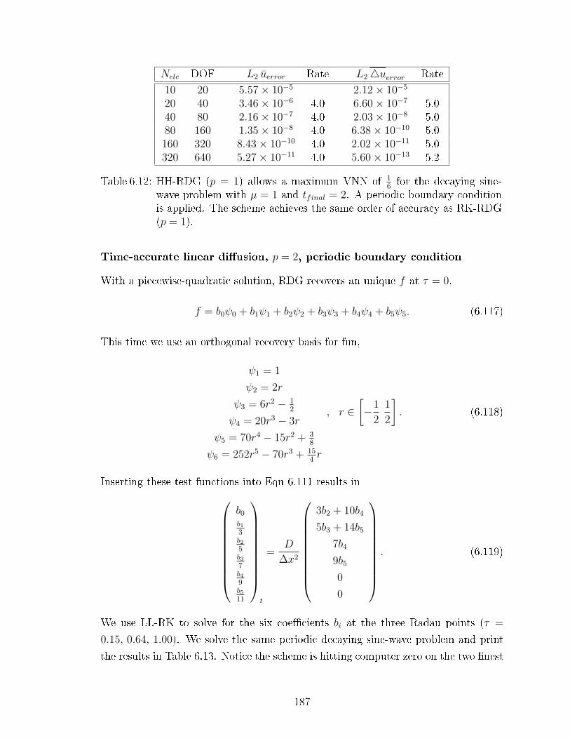
Nele DOF L2 uerror Rate L24uerror Rate
10 20 5.57× 10⁻⁵ 2.12× 10⁻⁵
20 40 3.46× 10⁻⁶ 4.0 6.60× 10⁻⁷ 5.040 80 2.16× 10⁻⁷ 4.0 2.03× 10⁻⁸ 5.080 160 1.35× 10⁻⁸ 4.0 6.38× 10⁻¹⁰ 5.0160 320 8.43× 10⁻¹⁰ 4.0 2.02× 10⁻¹¹ 5.0320 640 5.27× 10⁻¹¹ 4.0 5.60× 10⁻¹³ 5.2
Table 6.12: HH-RDG (p = 1) allows a maximum VNN of 16for the decaying sine-
wave problem with µ = 1 and tfinal = 2. A periodic boundary conditionis applied. The scheme achieves the same order of accuracy as RK-RDG(p = 1).
Time-accurate linear diusion, p = 2, periodic boundary condition
With a piecewise-quadratic solution, RDG recovers an unique f at τ = 0,
f = b0ψ0 + b1ψ1 + b2ψ2 + b3ψ3 + b4ψ4 + b5ψ5. (6.117)
This time we use an orthogonal recovery basis for fun,
ψ1 = 1
ψ2 = 2r
ψ3 = 6r2 − 12
ψ4 = 20r3 − 3r
ψ5 = 70r4 − 15r2 + 38
ψ6 = 252r5 − 70r3 + 154r
, r ∈[−1
2
1
2
]. (6.118)
Inserting these test functions into Eqn 6.111 results in
b0
b13b25b37b49b511
t
=D
∆x2
3b2 + 10b4
5b3 + 14b5
7b4
9b5
0
0
. (6.119)
We use LL-RK to solve for the six coecients bi at the three Radau points (τ =
0.15, 0.64, 1.00). We solve the same periodic decaying sine-wave problem and print
the results in Table 6.13. Notice the scheme is hitting computer zero on the two nest
187
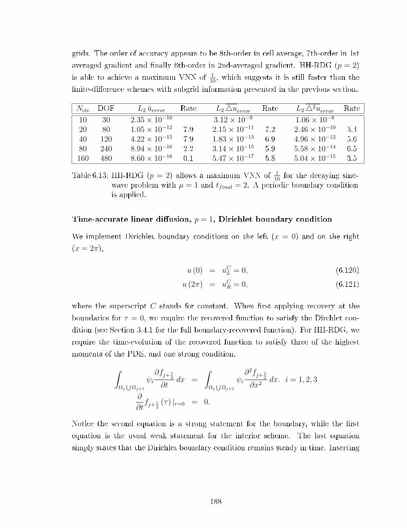
grids. The order of accuracy appears to be 8th-order in cell average, 7th-order in 1st
averaged gradient and nally 6th-order in 2nd-averaged gradient. HH-RDG (p = 2)
is able to achieve a maximum VNN of 110, which suggests it is still faster than the
nite-dierence schemes with subgrid information presented in the previous section.
Nele DOF L2 uerror Rate L24uerror Rate L242uerror Rate
10 30 2.35× 10⁻¹⁰ 3.12× 10⁻⁹ 1.06× 10⁻⁸
20 80 1.05× 10⁻¹² 7.9 2.15× 10⁻¹¹ 7.2 2.46× 10⁻¹⁰ 5.440 120 4.22× 10⁻¹⁵ 7.9 1.83× 10⁻¹³ 6.9 4.96× 10⁻¹² 5.680 240 8.94× 10⁻¹⁶ 2.2 3.14× 10⁻¹⁵ 5.9 5.58× 10⁻¹⁴ 6.5160 480 8.60× 10⁻¹⁶ 0.1 5.47× 10⁻¹⁷ 5.8 5.04× 10⁻¹⁵ 3.5
Table 6.13: HH-RDG (p = 2) allows a maximum VNN of 110
for the decaying sine-wave problem with µ = 1 and tfinal = 2. A periodic boundary conditionis applied.
Time-accurate linear diusion, p = 1, Dirichlet boundary condition
We implement Dirichlet boundary conditions on the left (x = 0) and on the right
(x = 2π),
u (0) = uCL = 0, (6.120)
u (2π) = uCR = 0, (6.121)
where the superscript C stands for constant. When rst applying recovery at the
boundaries for τ = 0, we require the recovered function to satisfy the Dirchlet con-
dition (see Section 3.4.1 for the full boundary-recovered function). For HH-RDG, we
require the time-evolution of the recovered function to satisfy three of the highest
moments of the PDE, and one strong condition,∫Ωj⋃
Ωj+1
ψi∂fj+ 1
2
∂tdx =
∫Ωj⋃
Ωj+1
ψi∂2fj+ 1
2
∂x2dx. i = 1, 2, 3
∂
∂tfj+ 1
2(τ) |r=0 = 0.
Notice the second equation is a strong statement for the boundary, while the rst
equation is the usual weak statement for the interior scheme. The last equation
simply states that the Dirichlet boundary condition remains steady in time. Inserting
188

f =∑4
i=1 biri for the left Dirichlet boundary results in
b0
b02
+ b13
+ b24
+ b35
b03
+ b14
+ b25
+ b36
b04
+ b15
+ b26
+ b37
t
=
uCL
D∆x2 (b2 + 2b3)D
∆x2
(2b23
+ 3b32
)D
∆x2
(b22
+ 6b35
)
. (6.122)
Similarly, for the right Dirichlet boundary condition,b0
− b02
+ b13− b2
4+ b3
5b03− b1
4+ b2
5− b3
6
− b04
+ b15− b2
6+ b3
7
t
=
uCR
D∆x2 (−b2 + 2b3)D
∆x2
(2b23− 3b3
2
)D
∆x2
(− b2
2+ 6b3
5
)
. (6.123)
The results of HH-RDG (p = 1) with full boundary-recovered function are presented
in Table 6.14.
Nele DOF L2 uerror Rate L24uerror Rate
10 20 5.57× 10⁻⁵ 3.37× 10⁻⁵
20 40 3.45× 10⁻⁶ 4.0 1.06× 10⁻⁶ 5.040 80 2.16× 10⁻⁷ 4.0 3.53× 10⁻⁸ 4.980 160 1.35× 10⁻⁸ 4.0 1.08× 10⁻⁹ 5.0160 320 8.43× 10⁻¹⁰ 4.0 3.18× 10⁻¹¹ 5.1320 640 5.27× 10⁻¹¹ 4.0 1.52× 10⁻¹² 4.4
Table 6.14: HH-RDG (p = 1) obtains a maximum VNN of 16for the decaying sine-
wave problem with µ = 1 and tfinal = 2. Dirichlet boundary conditionson both sides are satised with full boundary-recovered function.
We now demonstrate the downside of doing things wrongly at the boundary. Let
us naively have f evolve via LL-RK at the boundary element without satisfying the
boundary condition, hence the local evolution equation is the same as the one for the
interior scheme. For f on the left side of the numerical domain,b0 + b1
2+ b2
3+ b3
4b02
+ b13
+ b24
+ b35
b03
+ b14
+ b25
+ b36
b04
+ b15
+ b26
+ b37
t
=D
∆x2
2b2 + 3b3
b2 + 2b3
2b23
+ 3b32
b22
+ 6b35
, (6.124)
189

and for f on the right side of the numerical domain,b0 − b1
2+ b2
3− b3
4
− b02
+ b13− b2
4+ b3
5b03− b1
4+ b2
5− b3
6
− b04
+ b15− b2
6+ b3
7
t
=D
∆x2
2b2 − 3b3
−b2 + 2b3
2b23− 3b3
2
− b22
+ 6b35
. (6.125)
One might immediately question whether f will satisfy the boundary condition during
a local evolution. Table 6.15 shows this naive scheme does satisfy the boundary
condition, however the scheme suers a 50% time-step restriction.
Nele DOF L2 uerror Rate L24uerror Rate
10 20 2.13× 10⁻⁵ 2.09× 10⁻⁵
20 40 1.73× 10⁻⁶ 3.6 5.53× 10⁻⁷ 5.240 80 1.22× 10⁻⁷ 3.8 1.69× 10⁻⁸ 5.080 160 8.01× 10⁻⁸ 3.9 5.23× 10⁻¹⁰ 5.0160 320 5.14× 10⁻¹⁰ 4.0 1.63× 10⁻¹¹ 5.0320 640 3.26× 10⁻¹¹ 4.0 5.07× 10⁻¹³ 5.0
Table 6.15: Naive Dirichlet boundary scheme. HH-RDG (p = 1) with a maximumVNN of 1
12for a decaying sine-wave problem with µ = 1 and tfinal = 2.
The naive method suers reduction in both accuracy and VNN.
Fourier Analysis of HH-RDG for linear diusion, p = 1, 2
In order to rid critics of all skeptism, we performed Fourier analysis on the the HH-
RDG (p = 1) scheme to determine the stability of the scheme. We rewrite the nal
update equations for the two variables in matrix form,
∂
∂t(~uj) = (MLMCMR)
T−1 (~uj)
I (~uj)
T+1 (~uj)
, (6.126)
ML =
(9r4− 15r2
25r4− 15r2
245r2
2− 15r
433r2
2− 7r
4
), (6.127)
MC =
(15r2 − 9r
2+ 1 0
0 57r2 − 23r2
+ 1
), (6.128)
MR =
(9r4− 15r2
215r2
2− 5r
415r4− 45r2
233r2
2− 7r
4
), (6.129)
190

where r is the Von Neumann number. We translate the shift operators into Fourier
modes,
∂∂t
(~uj) = 15r2 − 9r2
+ 2e−iβ(
9r4− 15r2
2
)+ 1 e−iβ
(5r4− 15r2
2
)+ e−iβ
(15r2
2− 5r
4
)e−iβ
(15r4− 45r2
2
)+ e−iβ
(45r2
2− 15r
4
)57r2 − 23r
2+ 2e−iβ
(33r2
2− 7r
4
)+ 1
(~uj) .
The two eigenvalues associated with the matrix above read,
λ1 =1
2
(−30r2e−iβ + 30r2 + 9re−iβ − 9r + 2
), (6.130)
λ2 =1
2e−iβ
(114r2eiβ + 66r2 − 23reiβ − 7r + 2eiβ
). (6.131)
Stability requires the magnitude of the eigenvalues as a function of r must not exceed
unity for any β. Figure 6.10 shows the polar plot of the eigenvalues for r = 16and
r = 15. The two eigenvalues overlap each other for r = 1
6, and remains bounded within
the unit circle. However, for r larger than 16, one of the eigenvalue lies outside of the
unit circle implying instability. We go through the same analysis procedure for p = 2
and only present the nal results in Figure 6.11.
-1.0 -0.5 0.0 0.5 1.0-1.0
-0.5
0.0
0.5
1.0
Re Λ
ImΛ
r=16
-1.0 -0.5 0.0 0.5 1.0 1.5
-1.0
-0.5
0.0
0.5
1.0
Re Λ
ImΛ
r=15
Figure 6.10: Polar plots in the complex plane of the two eigenvalues of the updatematrix of HH-RDG (p = 1) scheme. The dashed line indicates the sta-bility boundary. For r = 1
6, the two eigenvalues coincide. For anything
larger than r = 16, one eigenvalue lies outside of the stability domain.
191

-1.0 -0.5 0.0 0.5 1.0-1.0
-0.5
0.0
0.5
1.0
Re Λ
ImΛ
r=110
-3 -2 -1 0 1
-2
-1
0
1
2
Re Λ
ImΛ
r=18
Figure 6.11: Polar plots in the complex plane of the two eigenvalues of the updatematrix of HH-RDG (p = 2) scheme. The dashed line indicates the sta-bility boundary. For r = 1
10, the three eigenvalues remain bounded by
the stability circle. For r larger than 110, one eigenvalue lies outside of
the stability domain.
Summary of HH-RDG for diusion
We have formulated the HH-RDG scheme for time-accurate diusion problems. Nu-
merical experiments show that the accuracy obtained by HH-RDG is on par with
RK-RDG. Although a direct comparison in total CPU time is not available, HH-RDG
requires many fewer binary-recovery operations than RD-RDG. We also demonstrated
how to incorporate boundary conditions into the HH-RDG. Fourier analysis for p = 1
and 2 conrms the maximum VNN found in numerical experiments. The journey to
develop the HH-RDG scheme has been a long one due to the dience in advection
and diusion operators. We are now ready to observe the behavior of the combined
HH-DG advection and diusion operators.
6.4 HH-DG linear advection-diusion in 1-D
Most literature in CFD lumps together advection and diusion terms and then mag-
ically approximates them dierently (as with LDG in Section 1.4.2). Throughout
the entire span of this thesis, we emphasize advection and diusion are completely
dierent physical phenomena and require completely dierent numerical approaches.
192

This section utilizes the HH-DG upwind operator for advection and the HH-RDG
operator for diusion to solve for dierent parts of the governing equation. We ac-
centuate the fact that our operators are completely independent of each other, and
require no ad-hoc parameters for stability or error tuning.
We solve the linear advection of the form,
ut + aux = Duxx, (6.132)
where a is the constant advection speed and D is the constant diusion coecient.
The update equation is obtained by testing the equation in both space and time, after
suitable integrations by parts (once for advection term and twice for diusion term),∫∫vut dxdt = −a
∫∫vux dxdt+ µ
∫∫vuxx dxdt,
= −a∫ (∮
vu dx−∫vxu dx
)dt
+D
∫ (∮(vux − vxu) dx+
∫vxxu dx
)dt. (6.133)
We discretize by applying the equation to each element Ωj and replacing global co-
ordinates with local coordinates in Eqn 6.5,
∫Ωj
v(un+1 − un
)dξ = −a∆t
∆x
∫ ([vu] |10 −
∫Ωj
vξu dξ
)dτ︸ ︷︷ ︸
advection
+D∆t
∆x2
∫ ([vuξ − vξu] |10 +
∫Ωj
vξξu dξ
)dτ︸ ︷︷ ︸
diusion
. (6.134)
Notice all the terms on the RHS appear to be only a function of space because we
have yet to implement our new ideas. For the advection terms, we apply Hancock's
observation and replace the solution in the surface integral with ust (ξ, τ); following
Huynh we compute the volume integral with un+τ . For the diusion terms, we replace
the solution in the surface integral with f st(τ) and in the volume integral with un+τ .
The weak space-time expansion for u is obtained by using LL-RK (see Eqn 6.17) on
193

the following system,
∆x
∫vut dξ =
(−a(
[vu] |10 −∫
Ωj
vξu dξ
)+
D
∆x
([vuξ − vξu] |10 +
∫Ωj
vξξu dξ
)).
(6.135)
In contrast, the weak space-time expansion for f is acquired by sharing moments with
the original governing equation,∫Ωj⋃
Ωj+1
ψ ft,j+ 12dx =
∫Ωj⋃
Ωj+1ψ
(−afx,j+ 1
2+Dfxx,j+ 1
2
)dx. (6.136)
The space-time solutions of both u and f are advanced to the Radau points in time
and then stored. The true purpose of this short study is to analyze the relation-
ship between the advection and diusion operators. Physically speaking, when the
advection phenomenon dominates the diusion phenomenon, we expect the order of
accuracy and time-step restriction to approach those of the advection operator. Like-
wise, we expect the opposite when diusion dominates the ow. The balance between
advection and diusion is described by the global Péclet number,
PeG =aL
D, (6.137)
where L is the characteristic length scale of the physical domain of interest. The
global Péclet number approaches zero (PeG → 0) for diusion-dominated problems,
and innity (PeG →∞) for advection-dominated problems. We also dene a local
Péclet number, which is more relevant to our numerical studies,
PeL =a∆x
D, (6.138)
where the characteristic length scale is now the width of the element. A grid-
renement study is always performed with constant global Péclet number.
The local Péclet number is also the ratio between the CFL number and VNN,
PeL =
(a∆t
∆x
)/
(D∆t
∆x2
)=a∆x
D, (6.139)
and appears in the stability condition of explicit advection-diusion schemes. Take,
e.g, the simplest upwind-advection/central-diusion dierence scheme; a Fourier anal-
194
ysis yields the stability condition
CFL + 2VNN ≤ 1, (6.140)
ora∆t
∆x+
2D∆t
∆x2≤ 1. (6.141)
This can be reduced to:
∆t ≤ ∆x
a
PeL2 + PeL
. (6.142)
Let us vary PeL by varying ∆x at constant a and D. For large PeL (large ∆x) Eqn
6.142 approaches the CFL condition, and ∆t ∼ ∆x. For small PeL (small ∆x), ∆t
becomes proportional to ∆x2 and the condition reduces to VNN < 12. For the HH-DG
schemes we shall assume the following form of the stability condition:
1
VNN· D∆t
∆x2+
1
CFL· a∆t
∆x≤ 1 · CAdv-Di, (6.143)
where CFL = 1 for all HH-DG advection operator using upwind ux, and VNN is the
highest stable Von Neumann number for pure diusion determined from the previous
sections. The coecient CAdv-Di is a safety factor. Solving for ∆t gives
∆t ≤ CAdv-Di
1VNN· D
∆x2 + 1CFL
a∆x
. (6.144)
In pure diusion or advection cases, the constant coecient CAdv-Di equals 1, however
it is numerically found that for this value accuracy is reduced for mixed advection-
diusion problems. Simply setting CAdv-Di ≤ 1 recovers the desired order of accuracy.
We will next look at detailed derivations for piecewise-linear (p = 1) and piecewise-
quadratic (p = 2).
6.4.1 Piecewise-linear & piecewise-quadratic HH-DG for lin-
ear advection-diusion equation
Perhaps one of the greatest advantages of using orthogonal basis functions is that the
update equations of the moments become independent of each other (on the LHS).
For example, this section hits two birds with one stone by deriving the update equa-
tions for a piecewise-quadratic scheme: one easily gets the piecewise-linear scheme by
setting all appearances of ∆2u to zero. Let the P 2 polynomial space be spanned by
195
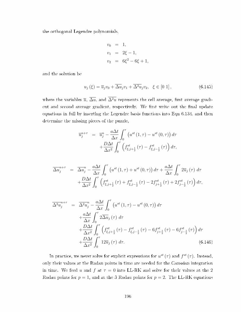
the orthogonal Legendre polynomials,
v0 = 1,
v1 = 2ξ − 1,
v2 = 6ξ2 − 6ξ + 1,
and the solution be
uj (ξ) = ujv0 + ∆ujv1 + ∆2ujv2, ξ ∈ [0 1] , (6.145)
where the variables u, ∆u, and ∆2u represents the cell average, rst average gradi-
ent and second average gradient, respectively. We rst write out the nal update
equations in full by inserting the Legendre basis functions into Eqn 6.134, and then
determine the missing pieces of the puzzle,
un+τj = unj −
a∆t
∆x
∫ τ
0
(ust (1, τ)− ust (0, τ)
)dτ
+D∆t
∆x2
∫ τ
0
(f stξ,j+ 1
2(τ)− f st
ξ,j− 12
(τ))dτ,
∆un+τ
j = ∆un
j −a∆t
∆x
∫ τ
0
(ust (1, τ) + ust (0, τ)
)dτ +
a∆t
∆x
∫ τ
0
2uj (τ) dτ
+D∆t
∆x2
∫ τ
0
(f stξ,j+ 1
2(τ) + f st
ξ,j− 12
(τ)− 2f stj+ 1
2(τ) + 2f st
j− 12
(τ))dτ,
∆2un+τ
j = ∆2un
j −a∆t
∆x
∫ τ
0
(ust (1, τ)− ust (0, τ)
)dτ
+a∆t
∆x
∫ τ
0
2∆uj (τ) dτ
+D∆t
∆x2
∫ τ
0
(f stξ,j+ 1
2(τ)− f st
ξ,j− 12
(τ)− 6f stj+ 1
2(τ)− 6f st
j− 12
(τ))dτ
+D∆t
∆x2
∫ τ
0
12uj (τ) dτ. (6.146)
In practice, we never solve for explicit expressions for ust (τ) and f st (τ). Instead,
only their values at the Radau points in time are needed for the Gaussian integration
in time. We feed u and f at τ = 0 into LL-RK and solve for their values at the 2
Radau points for p = 1, and at the 3 Radau points for p = 2. The LL-RK equations
196

for ust are very similar to the ones above, except there is no integration in time, and
all uxes are obtained from inner element values,
uj,t = − a
∆x(u (1)− u (0)) +
D
∆x2(uξ (1)− uξ (0)) ,
(∆uj
)t
= − a
∆x(u (1) + u (0))
+a
∆x(2uj) +
D
∆x2(uξ (1) + uξ (0)− 2u (1) + 2u (0)) ,
(∆2uj
)t
= − a
∆x(u (1)− u (0))
+a
∆x
(2∆uj
)+
D
∆x2(uξ (1)− uξ (0)− 6u (1)− 6u (0))
+D
∆x2(12uj) . (6.147)
We get the p = 1 update equations by setting ∆2u to zeros wherever it appears.
The same procedure follows for f st. Interface recovery generates a smooth quintic
polynomial at the interface with 6 unique coecients,
fj+ 12
= b0,j+ 12+b1,j+ 1
2r+b2,j+ 1
2r2+b3,j+ 1
2r3+b4,j+ 1
2r4+b5,j+ 1
2r5, r ∈ [−1
2
1
2], (6.148)
where r = 0 is the interface; it must satisfy 6 moments of the dierential form of the
governing equation. The result for r = 0 reads,
ft = 0! b0,t = −a (b1) +D
∆x(2b2) , (6.149)
ftt = 1! b1,t = −a (2b2) +D
∆x(3b3) , (6.150)
ft(3) = 2! b2,t = −a (6b3) +D
∆x(12b4) , (6.151)
ft(4) = 3! b3,t = −a (24b4) +D
∆x(60b5) , (6.152)
197
ft(5) = 4! b4,t = −a (120b5) , (6.153)
ft(6) = 5! b5,t = 0. (6.154)
These equations can easily be modied for p = 1 by setting b4 and b5 to zero. With
all pieces of the puzzles in hand, we proceed to test our HH-DG advection-diusion
operators for time-dependent problems.
6.4.2 Numerical results for linear advection-diusion with HH-
DG
We solve the simple time-dependent problem of a decaying sine wave,
u (t) = e−k2Dtsin k (x− at) . (6.155)
Observe the solution becomes zero as t → ∞. Let t = 0 and k = 1 be the initial
condition, and let t = 1 be the nal time. Note this is the same test case used by
Cockburn and Shu[8] to test LDG. We solve this equation for various values of the
Péclet number; the numerical results for p = 1 are presented in Figure 6.12. The
lower left corner is diusion dominated, while the upper right corner is advection
dominated; the order of accuracy transitions from 4 to slightly below 3 between these
corners. We observe the order of accuracy is roughly constant along the dashed lines
representing constant local Péclet number.
198

0.02 0.04 0.08 0.16 0.3210
−6
10−4
10−2
100
102
104
∆x
Pe G
44444
44444
44444
44444
3.64.43.84.23.9
3.63.83.74.13.2
3.13.13.33.63.5
2.82.72.82.93.1
2.42.52.72.72.7
2.52.62.52.52.5
Figure 6.12: HH-DG for linear advection-diusion problem, p = 1. Dashed line rep-resents constant cell Péclet number. The order of accuracy graduallytransitions from 4 at the bottom left corner to roughly 3 at the top rightcorner.
6.4.3 Fourier analysis of HH-DG for linear advection diusion
This section briey covers the Fourier analysis of HH-DG for linear advection diusion
for p = 1 and p = 2. The exact update matrices for p = 1 based on 3-stage LL-RK
and two Radau points, and for p = 2 based on 5-stage LL-RK and three Radau
points, are too extensive to be presented because the number of terms in the matrix
elements increases with the product of the number of LL-RK stages and the number
of Radau points. The following gures present the polar plots of the eigenvalues of the
update matrices for a range of Péclet numbers. The time step is chosen in accordance
with Eqn 6.144, with VNN = 16for p = 1, VNN = 1
10for p = 2 and (nominally)
CAdv-Di = 1. It is seen that for Pe ≈ 1 the stability of the method is reduced,
requiring a reduction of CAdv-Di (see Figures 6.16-6.17). For p = 1 this reduction is
mild (CAdv-Di = 0.9375); for p = 2 it is severe (CAdv-Di = 0.20). It is not clear what
causes this reduction in the stable time-step range when advection and diusion are
equally important; this remains a subject of future investigation.
199
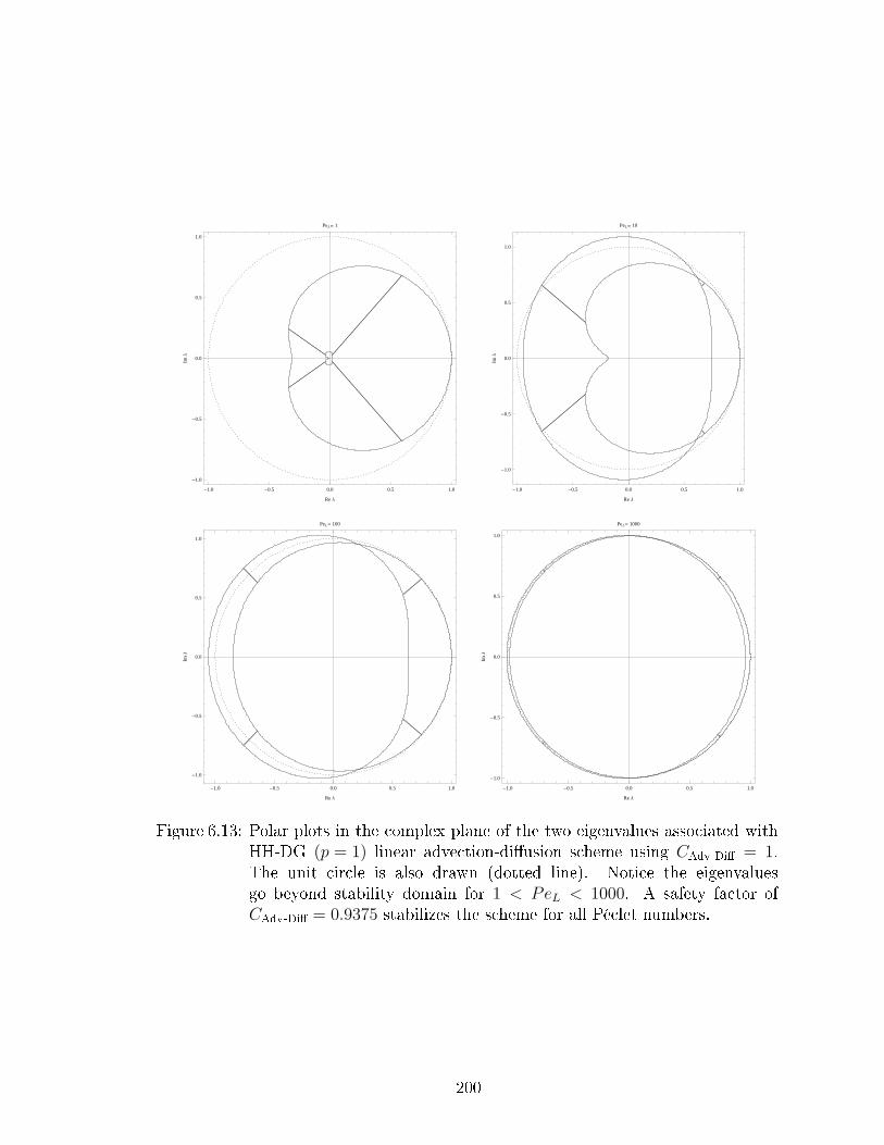
-1.0 -0.5 0.0 0.5 1.0
-1.0
-0.5
0.0
0.5
1.0
Re Λ
ImΛ
PeL= 1
-1.0 -0.5 0.0 0.5 1.0
-1.0
-0.5
0.0
0.5
1.0
Re ΛImΛ
PeL= 10
-1.0 -0.5 0.0 0.5 1.0
-1.0
-0.5
0.0
0.5
1.0
Re Λ
ImΛ
PeL= 100
-1.0 -0.5 0.0 0.5 1.0
-1.0
-0.5
0.0
0.5
1.0
Re Λ
ImΛ
PeL= 1000
Figure 6.13: Polar plots in the complex plane of the two eigenvalues associated withHH-DG (p = 1) linear advection-diusion scheme using CAdv-Di = 1.The unit circle is also drawn (dotted line). Notice the eigenvaluesgo beyond stability domain for 1 < PeL < 1000. A safety factor ofCAdv-Di = 0.9375 stabilizes the scheme for all Péclet numbers.
200

-1.0 -0.5 0.0 0.5 1.0
-1.0
-0.5
0.0
0.5
1.0
Re Λ
ImΛ
PeL= 0.001
-1.0 -0.5 0.0 0.5 1.0
-1.5
-1.0
-0.5
0.0
0.5
1.0
1.5
Re Λ
ImΛ
PeL= 0.1
-15 000 -10 000 -5000 0 5000 10 000 15 000
-6000
-4000
-2000
0
2000
4000
6000
Re Λ
ImΛ
PeL= 100
-1.0 -0.5 0.0 0.5 1.0
-1.0
-0.5
0.0
0.5
1.0
Re Λ
ImΛ
PeL= 1 x 10⁹
Figure 6.14: Polar plots in the complex plane of the three eigenvalues associated withHH-DG (p = 2) linear advection-diusion scheme using CAdv-Di = 1.The unit circle is also drawn (dotted line). Notice the eigenvalues gobeyond the stability domain for 10−3 < PeL < 108. A safety factor ofCAdv−Diff = 0.2 stabilizes the scheme for all Péclet numbers.
201

-1.0 -0.5 0.0 0.5 1.0
-1.0
-0.5
0.0
0.5
1.0
Re Λ
ImΛ
PeL= 100
-1.0 -0.5 0.0 0.5 1.0
-1.0
-0.5
0.0
0.5
1.0
Re Λ
ImΛ
PeL= 1 x 10⁵
Figure 6.15: After applying a safety factor of CAdv−Diff = 0.2, the three eigenval-ues associated with HH-DG (p = 2) linear advection-diusion scheme liewithin the stability domain for all range of Péclet number.
6.5 Chapter summary
We have extended Huynh's moment scheme beyond piecewise linear (HH-DG), and
developed a new space-time diusion scheme for DG (HH-RDG). Common to both
methods is the use of a numerical LL-RK procedure to approximate the analytical CK
procedure, and the use of a hierchical procedure to include the newest information
into the volume integral. We have shown once more that what works for advection
does not work for diusion. In HH-DG the solution evolves in time, while in HH-RDG
both the solution and the recovered function evolve in time.
The HH-DG scheme for advection is demonstrated to be the exact shift operator
with CFL = 1 for linear problems. When applied to the Euler equations, HH-DG ap-
pears to be 3rd-order accurate for p = 1 (as already demonstrated in [17]); the results
for p = 2 are currently unsatisfactory and will be the subject of future investigation.
The HH-RDG scheme for diusion is still in its infant stage of development; we
have only demonstrated its ability for scalar linear diusion problems. The results so
far look promising. In comparison to RK-RDG, HH-RDG achieves the same order of
accuracy with much fewer ux evaluations and a higher VNN number. Our next goal
is to extend HH-RDG to nonlinear diusion, incorporating the solution enhancement
techniques of Section 3.5.1.
The study on the combined HH-DG and HH-RDG schemes for advection-diusion
202
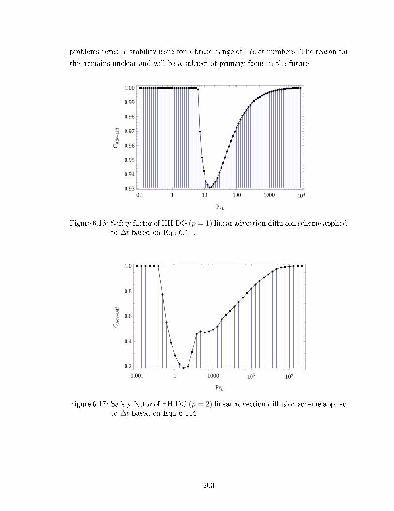
problems reveal a stability issue for a broad range of Péclet numbers. The reason for
this remains unclear and will be a subject of primary focus in the future.
0.1 1 10 100 1000 1040.93
0.94
0.95
0.96
0.97
0.98
0.99
1.00
PeL
CA
dv-
Dif
f
Figure 6.16: Safety factor of HH-DG (p = 1) linear advection-diusion scheme appliedto ∆t based on Eqn 6.144
0.001 1 1000 106 109
0.2
0.4
0.6
0.8
1.0
PeL
CA
dv-
Dif
f
Figure 6.17: Safety factor of HH-DG (p = 2) linear advection-diusion scheme appliedto ∆t based on Eqn 6.144
203

CHAPTER VII
Conclusions
Our research objectives have always been to design schemes that are conceptually
easy to understand, and a quantum level better than existing schemes. We hope
we have stayed true to our design principle and entertained our reader thus far.
This thesis details the growth of two new and exciting numerical methods: interface-
centered recovery-based DG (RDG) and Hancock-Huynh DG (HH-DG). The funda-
mental ideas behind both schemes arrive from an engineering perspective; none of
our schemes are based on facilitating or reducing the number of pages of mathemat-
ical proofs. RDG is a diusion operator for DG where the basis idea is to recover
a smooth solution from the discontinuous ones. The order of accuracy and stability
region of RDG are unsurpassed by any current DG diusion schemes. HH-DG is a
space-time scheme that sets itself apart from the popular Runge-Kutta DG (RK-DG)
with equal or smaller number of ux evaluations, larger time-steps, and lower memory
requirement. In fact, HH-DG is the exact shift operator for advection problems.
7.1 Summary
This author would like to honor Van Leer & Nomura for inventing the recovery
concept[44] in 2005, and Huynh for successfully porting Hancock's version of Van
Leer's scheme III into the DG framework[17] in 2006. Their work lays the foundation
for the topics covered in this thesis. The major contributions include:
• Ways to reduce the condition number for binary recovery in a numerical scheme.
We showed the condition number for solving the recovery equations is highly
dependent on the choice of basis for the solution and the test functions. A
combination of an orthogonal basis with a preconditioner will greatly reduce
204

the condition number.
• The concept of the smooth recovery basis (Section 2.4 and [43, 45]), which
relates the discontinuous solution to the smooth solution, provides a mechanism
to unify the treatment of advection and diusion. The smooth recovery basis is
designed to have the same solution coecients as the discontinuous solutions.
One can use the discontinuous basis for the advection operator, and the smooth
recovery basis for the diusion operator.
• Stability proofs for the classic RDG-2x and the naive RDG-1x are provided in
the end of Chapter 2. We proved the stability of these schemes for nonlinear
diusion problems with both Dirichlet and Neumann problems.
• We further investigate the stability and accuracy of various RDG schemes via
Fourier analysis. Chapter 3 provides both analytical and numerical Fourier anal-
yses. Our investigation allowed us to better understand errors in DG schemes;
there are projection and evolution errors. One must carefully design a scheme
to minimize both! We showed RDG has the smallest evolution error compared
with other schemes, i.e., the(σ, µ)-family and LDG.
• In order to see RDG's performance in relation to other diusion schemes, we
analyzed a venerable family of diusion schemes: the (σ, µ)-family for p = 1 (see
Section 3.3.3 and [42]). We were able to discover interesting lines and regions in
the (σ, µ)-plane, and eventually new (σ, µ)-schemes with fast convergence rates
and modest accuracy. We designed an RDG scheme, RDG-1xf , to t into the
(σ, µ)-framework, and showed this scheme to be the best in the family. This
study also shows that RDG-2x is dierent from the (σ, µ)-family, which leads
to our next important discovery.
• We expressed RDG-2x in terms of penalty-like (or bilinear) terms in Section
3.3.5. RDG-2x automatically generates higher-order bilinear terms as p in-
creases, with corresponding coecients. This is completely dierent from the
traditionally penalty method where the number of bilinear terms is xed re-
gardless of p and the corresponding coecients are chosen in a rather ad-hoc
manner.
• Our initial research was mostly focused on the theoretical analysis of RDG for
the scalar linear diusion equation. Extending RDG to nonlinear diusion re-
quired us to refocus on algorithm development. In order to handle nonlinear
205

terms, we introduced a solution-enhancement technique in Section 3.5 that in-
creases the accuracy of the evaluation of the volume integral appearing in the
RDG-1x formulation. Solution enhancement is achieved by reusing information
from the recovered functions to increase the order of the solution space within
a cell.
• We greatly increased the scope of RDG by extending the recovery concept from
1-D to 2-D in Chapter 4. Although the recovery concept remains the same, the
recovered functions at the domain boundaries require extra attention. We intro-
duced the full boundary-recovered and compact boundary-recovered functions
for Cartesian and unstructured triangular grids, respectively. We also studied
the performance of RDG schemes on irregular triangular grids.
• In dealing with nonlinear problems for 2-D, the cross-derivative terms become
a new obstacle for RDG (see Section 4.2.3). The binary recovery procedure
creates a recovered function that is more accurate in the face-normal direc-
tion than the face-parallel direction. Having cross-derivative terms means high-
order accuracy is demanded in the face-parallel direction; in this regard we
introduce recovered-function enhancement to remedy the problem. The cur-
rent recovered-function-enhancement technique requires the enhanced solution
to create a higher-order recovered function. Unfortunately, this increases the
stencil size of RDG schemes as in RDG-1x++; RDG-1x++CO is an optimized
version for Cartesian grids with a smaller stencil. The numerical results for
RDG-1x++CO are reassuring; it achieves the same order of accuracy for non-
linear problems with cross derivatives as the classic RDG-2x for linear problems.
• We presented numerical results for the Runge-Kutta upwind-DG (RK-uDG)
for linear advection, RK-RDG for linear diusion, and the combined RK-uDG
and RK-RDG for linear advection-diusion equations. The study on the linear
advection-diusion equation is based on the Péclet number. For advection-
dominated problems, the order of accuracy approaches to that of RK-uDG, and
for diusion-dominated problems, the order of accuracy approaches that of RK-
RDG scheme. There is a smooth transition in the order of accuracy between
the two schemes when the Péclet number is of order unity.
• The extension of Huynh's moment scheme[17] to arbitrarily high order (HH-
DG in Section 6.2), while maintaining the perfect shift property. The ux
evaluation is based on the classic Hancock observation. The incorporation of
206

wave interaction within a cell is based on Huynh's treatment of the volume
integral in the moment scheme. The HH-DG scheme is remarkably fast due
to a CFL of unity, and relatively fast compared to RK-DG due to the reduced
number of ux evaluations per time step. We demonstrated HH-DG abilities
on both the linear advection and Euler equations; these results also conrm the
viability of replacing the analytical Cauchy-Kovalevskaya (CK) procedure with
a numerical one, the local linear Runge-Kutta (LL-RK) technique (see Section
6.2.1).
• The highly nonlinear extension of HH-DG to recovery (HH-RDG in Section 6.3).
What works for the gander does not work for the goose; it turns out diusion
requires a completely dierent approach as advection. In HH-DG, we apply LL-
RK to the solution to get a space-time expanded solution, but for HH-RDG, we
apply LL-RK to the recovered function to get a space-time expanded recovered
function. This has a major benet because only one binary-recovery operation
is needed at the beginning of a time step. We showed HH-RDG achieves the
same order of accuracy as RK-RDG with much fewer binary-recovery operations
while having the same Von Neumann numbers.
• We analyzed and tested the combined HH-DG and HH-RDG schemes for the
linear advection-diusion equation in Section 6.4. Unlike the combined RK-
uDG and RK-RDG schemes, the combined HH-DG/HH-RDG scheme suers a
time-step penalty for Péclet numbers around unity. The problem appears to be
growing worse for increasing p.
• The making of the poster History of CFD: Part II for Van Leer's AIAA Fluid
Dynamics Award lecture in 2010. The people and papers discussed in this award
lecture are directly related to the development of high-order advection schemes.
Van Leer's scheme III[37] is the groundwork for the current HH-DG scheme.
7.2 Future work
RDG and HH-DG are new schemes introduced into the world of DG. These new-
borns are still going through development and many important questions remain at
the end of this thesis. In order to address these issues, a list of future research topics
is listed below:
207

Figure
7.1:
History
ofCFDPartII:Courtesyof
Van
LeerandLo.
208
• The development of a compact RDG scheme for nonlinear problems with cross-
derivatives terms. The current nonlinear RDG schemes utilize a large stencil
that is not well suited for triangular grids or implicit time-marching schemes.
The use of a compact stencil will most likely decrease the accuracy, but increases
the speed of recovery since fewer equations are involved.
• We have yet to run numerical experiements on the full Navier-Stokes equations
with the combined RDG and uDG schemes. Although the combined scheme
worked well for linear advection-diusion, nothing is for certain in the fully
nonlinear case with shear terms.
• The results and analyses for HH-RDG are only for linear diusion. We wish
to incorporate solution- and recovered-function enhancements into HH-RDG to
handle nonlinear diusion problems.
• We wish to demonstrate local time-stepping with HH-DG. A major strength of
space-time DG methods is the ability to take local time steps in each cell to
reduce computational cost on grids with a large variation in cell size.
• Perhaps the most puzzling problem of HH-DG and HH-RDG is the reduction
in time step for Péclet numbers close to unity. Investigating and resolving this
issue is essential to turning these space-time DG methods into viable numerical
methods.
7.3 The eort: revisiting the River of Recovery
The thesis summary does not show the eort in achieving each of the goals listed.
Let us return to the River of Recovery in Section 1.6. The longest time and largest
eort was spent between the river source and the rst cascade. Although the diusion
equations we studied were linear, the analysis was hard enough and it simply took
time to get a feeling for DG methods for diusion. Crossing the nonlinearity cascade,
although a harder problem, took less time owing to the insight we had gathered
upstream. Crossing the cascades of the cross-derivatives was a similar challenge and
took a comparable amount of research time. The work on space-time DG, as depicted
in the upper side stream, started as a diversion during the second half of the research
period and was carried out with interruptions.
In retrospect the hardest-won results were three in number. In the rst place, the
use of solution enhancement, based on recycling recovery information, to overcome
209

inaccuracy of the volume integral caused by nonlinearity. Second-hardest was apply-
ing the ideas of the space-time DG method for advection to diusion. Thirdly, the
further use of binary recovery steps on top of the earlier solution enhancement, in
order to accurately represent cross-derivatives in the PDE.
At the end of this long journey down the river we recovered the eort spent in
the form of the joy of seeing the original concept of RDG mature into a collection of
methods that are suited for practical nonlinear diusion problems.
210

APPENDICES
211
APPENDIX A
Elements of Computational Fluid Dynamics
The purpose of this section is to focus on selected fundamental ideas of compu-
tational uid dynamics (CFD). These ideas include Gaussian integration, solution
projection, derivatives of primitive variables and implicit Radau integration.
A.1 Gaussian quadrature
There is not a single bread-and-butter solution when it comes to the evaluation of
nite integrals; the choice of an analytical or a numerical integration technique de-
pends on the situation. Analytical integration is preferred when the integrand is
simple and the code requires high precision. The integrand arising from a nonlinear
system of equations is frequently too complex for analytical integration; in this case,
a numerical technique is preferred.
The idea behind Gaussian quadrature is to express the nite integral of a function
as a weighted sum of the function at specic points,∫ b
a
f (x) dx =n∑i=1
wif (xi) , (A.1)
where xi is the Gaussian point and wi is the corresponding weight. In general, a
classical n-points Gaussian quadrature rule evaluates a polynomial of degree 2n − 1
exactly (see left diagram of Figure A.1). Note all the Gaussian points are located in
the interior of the integration domain. One can think of the number of Gaussian points
and their corresponding weights as degrees of freedom to represent a polynomial.
If we are to force the location of one Gaussian point to the boundary (as in the
212
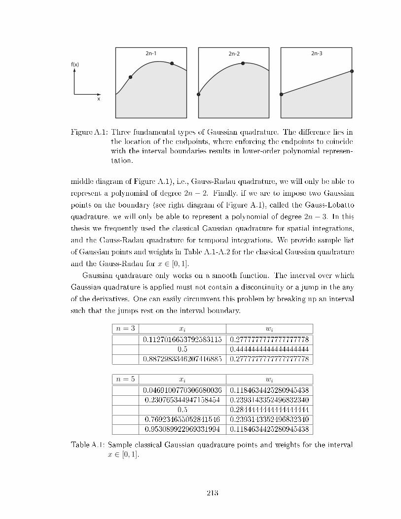
x
f(x)
2n-1 2n-2 2n-3
Figure A.1: Three fundamental types of Gaussian quadrature. The dierence lies inthe location of the endpoints, where enforcing the endpoints to coincidewith the interval boundaries results in lower-order polynomial represen-tation.
middle diagram of Figure A.1), i.e., Gauss-Radau quadrature, we will only be able to
represent a polynomial of degree 2n − 2. Finally, if we are to impose two Gaussian
points on the boundary (see right diagram of Figure A.1), called the Gauss-Lobatto
quadrature, we will only be able to represent a polynomial of degree 2n− 3. In this
thesis we frequently used the classical Gaussian quadrature for spatial integrations,
and the Gauss-Radau quadrature for temporal integrations. We provide sample list
of Gaussian points and weights in Table A.1-A.2 for the classical Gaussian quadrature
and the Gauss-Radau for x ∈ [0, 1].
Gaussian quadrature only works on a smooth function. The interval over which
Gaussian quadrature is applied must not contain a discontinuity or a jump in the any
of the derivatives. One can easily circumvent this problem by breaking up an interval
such that the jumps rest on the interval boundary.
n = 3 xi wi
0.1127016653792583115 0.27777777777777777780.5 0.4444444444444444444
0.8872983346207416885 0.2777777777777777778
n = 5 xi wi
0.0469100770306680036 0.11846344252809454380.230765344947158454 0.2393143352496832340
0.5 0.28444444444444444440.769234655052841546 0.23931433524968323400.953089922969331994 0.1184634425280945438
Table A.1: Sample classical Gaussian quadrature points and weights for the intervalx ∈ [0, 1].
213
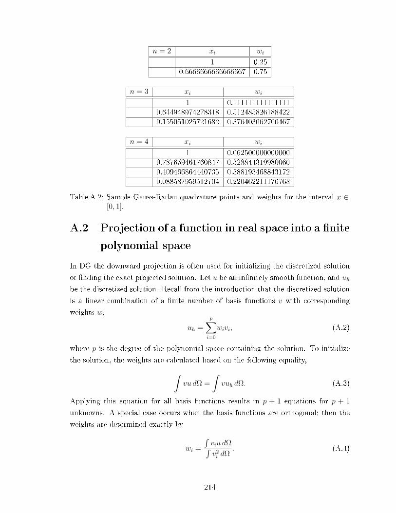
n = 2 xi wi
1 0.250.6666666666666667 0.75
n = 3 xi wi
1 0.1111111111111110.644948974278318 0.5124858261884220.155051025721682 0.376403062700467
n = 4 xi wi
1 0.0625000000000000.787659461760847 0.3288443199800600.409466864440735 0.3881934688431720.088587959512704 0.220462211176768
Table A.2: Sample Gauss-Radau quadrature points and weights for the interval x ∈[0, 1].
A.2 Projection of a function in real space into a nite
polynomial space
In DG the downward projection is often used for initializing the discretized solution
or nding the exact projected solution. Let u be an innitely smooth function, and uh
be the discretized solution. Recall from the introduction that the discretized solution
is a linear combination of a nite number of basis functions v with corresponding
weights w,
uh =
p∑i=0
wivi, (A.2)
where p is the degree of the polynomial space containing the solution. To initialize
the solution, the weights are calculated based on the following equality,∫vu dΩ =
∫vuh dΩ. (A.3)
Applying this equation for all basis functions results in p + 1 equations for p + 1
unknowns. A special case occurs when the basis functions are orthogonal; then the
weights are determined exactly by
wi =
∫viu dΩ∫v2i dΩ
. (A.4)
214
The term error is perhaps one of the most negligently used terminologies in DG
papers. If we compare solutions across dierent polynomial spaces, we called that the
projection error. If we compare solutions in the same polynomial space (as in this
thesis), we call it the evolution error. We dene the L2-norm of the projection error
to be
eL2,proj =
(Nele∑j=1
∫(uh,j − u)2 dΩj
Nele
) 12
, (A.5)
where Nele is the total number of cells. Here we are taking the dierence between the
innitely smooth solution with the discrete solution, which always results in an error
of order p+ 1. This leads us to a major observation: all DG schemes contain at least
a (p+ 1)-order projection error. This error is committed regardless of the numerical
scheme, and hence what dierentiates all numerical schemes from each other is the
evolution error. The L2-norm of the evolution error is dened to be
eL2,evol =
(Nele∑j=1
(∫v (uh,j − u) dΩj
)2
Nele
) 12
. (A.6)
Here we are comparing the downward projection of the exact solution with the discrete
solution. With our choice of Legendre basis, we obtain the evolution error of the cell
average if v = 1. Similarily, we obtain the evolution error of the rst average gradient
if v = 2ξ − 1. The following numerical experiment will illuminate the dierence
between projection and evolution errors.
Evolution error vs projection error
We consider three (σ, µ)-schemes (p = 1) from Section 3.3.3 to solve a steady-state
problem with a source term,
ut = uxx + 4π2sin (2πx) , (A.7)
and with Dirichlet boundary conditions,
u (0) = 1, (A.8)
u (1) = 0. (A.9)
The steady solution is
u (x,∞) = 1− x+ sin (2πx) . (A.10)
215
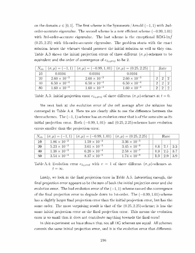
on the domain x ∈ [0, 1]. The rst scheme is the Symmetric/Arnold (−1, 1) with 2nd-
order-accurate eigenvalue. The second scheme is a new ecient scheme (−0.99, 1.01)
with 3rd-order-accurate eigenvalue. The last scheme is the exceptional RDG-1xf
(0.25, 2.25) with 4th-order-accurate eigenvalue. The problem starts with the exact
solution, hence the schemes should preserve the initial solution as well as they can.
Table A.3 shows the initial projection errors of three dierent (σ, µ)-schemes to be
equivalent and the order of convergence of eL2,proj to be 2.
Nele (σ, µ) = (−1, 1) (σ, µ) = (−0.99, 1, 01) (σ, µ) = (0.25, 2.25) Rate
10 0.0104 0.0104 0.010420 2.60× 10⁻³ 2.60× 10⁻³ 2.60× 10⁻³ 2 2 240 6.50× 10⁻⁴ 6.50× 10⁻⁴ 6.50× 10⁻⁴ 2 2 280 1.60× 10⁻⁴ 1.60× 10⁻⁴ 1.60× 10⁻⁴ 2 2 2
Table A.3: Initial projection error eL2,proj of three dierent (σ, µ)-schemes at t = 0.
We next look at the evolution error of the cell average after the solution has
converged in Table A.4. Here we are clearly able to see the dierence between the
three schemes. The (−1, 1)-scheme has an evolution error that is of the same size as its
initial projection error. Both (−0.99, 1, 01)- and (0.25, 2.25)-schemes have evolution
errors smaller than the projection error.
Nele (σ, µ) = (−1, 1) (σ, µ) = (−0.99, 1, 01) (σ, µ) = (0.25, 2.25) Rate
10 1.86× 10⁻² 1.59× 10⁻² 3.36× 10⁻⁵
20 5.23× 10⁻³ 3.61× 10⁻³ 3.45× 10⁻⁶ 1.8 2.1 3.340 1.38× 10⁻³ 6.20× 10⁻⁴ 2.58× 10⁻⁷ 1.9 2.5 3.780 3.54× 10⁻⁴ 8.37× 10⁻⁵ 1.74× 10⁻⁸ 1.9 2.9 3.9
Table A.4: Evolution error eL2,evol with v = 1 of three dierent (σ, µ)-schemes att =∞.
Lastly, we look at the nal projection error in Table A.5. Interesting enough, the
nal projection error appears to be the sum of both the initial projection error and the
evolution error. The bad evolution error of the (−1, 1)-scheme caused the convergence
of the nal projection error to degrade down to 1st-order. The (−0.99, 1.01)-scheme
has a slightly larger nal projection error than the initial projection error, but has the
same order. The most surprising result is that of the (0.25, 2.25)-scheme; it has the
same initial projection error as the nal projection error. This means the evolution
error is so small that it does not contribute anything towards the nal error!
In this experiment we have shown that not all DG schemes are equal. All schemes
commit the same initial projection error, and it is the evolution error that dierenti-
216

Nele (σ, µ) = (−1, 1) (σ, µ) = (−0.99, 1, 01) (σ, µ) = (0.25, 2.25) Rate
10 1.41× 10⁻¹ 8.68× 10⁻² 1.04× 10⁻²
20 7.32× 10⁻² 2.07× 10⁻² 2.60× 10⁻³ 0.9 2.0 2.040 3.69× 10⁻² 4.00× 10⁻³ 6.50× 10⁻⁴ 0.9 2.3 1.980 1.85× 10⁻² 6.80× 10⁻⁴ 1.60× 10⁻⁴ 1.0 2.5 1.9
Table A.5: Final projection error eL2,proj of three dierent (σ, µ)-schemes at t =∞.
ates the schemes. It is imperative to design a numerical scheme where the convergence
rate of the evolution error must be as least p+1. Yet once again we have shown RDG-
1xf to be superior.
A.3 Derivatives of primitive variable
In Chapter 5 we often need to express the derivatives of primitive variables in terms
of the conservative variables. Here we consider a simple example with conservative
variables ρ and m = ρu spanned by the Legendre basis in terms of ξ up to any
polynomial order:
ρ (ξ) = ρ+ ∆ρ (2ξ + 1) + ∆2ρ(6ξ2 − 6ξ + 1
)+ . . . , (A.11)
m (ξ) = m+ ∆m (2ξ + 1) + ∆2m(6ξ2 − 6ξ + 1
)+ . . . , (A.12)
and there derivatives are
∂ρ
∂ξ(ξ) = ∆ρ (2) + ∆2ρ (12ξ − 6) + . . . , (A.13)
∂m
∂ξ(ξ) = ∆m (2) + ∆2m (12ξ − 6) + . . . . (A.14)
We wish to obtain the derivative of u in terms of ξ. We rst express u in terms of
conservative variables,
u =m
ρ, (A.15)
and the derivative of u becomes
uξ = m∂ρ−1
∂ξ+
1
ρ
∂m
∂ξ. (A.16)
217
The term ∂ρ−1
∂ξrequires a substitution trick. Let q = 1
ρ, and then we use the chain
rule to obtain∂q
∂ξ=∂q
∂ρ
∂ρ
∂ξ, (A.17)
where ∂q∂ρ
= − 1ρ2 . This is an eective technique to obtain the derivative at point values
which are needed for Gaussian integration.
A.4 Implicit Radau Integration
The Radau points listed in Appendix A.1 are for explicit Radau integration. Explicit
means we acquire the numerical integral over the whole time interval τ ∈ [0 1] by a
correct linear combination of weights and function values at selected points. However,
in HH-DG we frequently need the integrate over a dierent interval, i.e., τ ∈ [0 τk],
where τk is any Radau point less than unity. Naively one can normalized another
set of Radau points to t into τ ∈ [0 τk], resulting in more ux evaluations in the
new sub-interval. This trick, donated by Dr. Huynh, circumvents this problem is to
t a smooth function through the original Radau points over the interval τ ∈ [0 1].
We then integrate the tted function over the sub-intervals τ ∈ [0 τk] to acquire the
proper function weights based on the function values at the original Radau points.
This is important because we reuse the information we already have and avoid extra
ux evaluations, making this an ecient numerical technique.
Consider an arbitrary function to be numerical evaluated,∫ τk
0
f (τ) dτ. (A.18)
If we have n Radau points, we can reconstruct a polynomial of degree n− 1, f (τ) =
a0 + a1τ + a2τ2 + · · ·+ an−1τ
n−1, on the interval τ = [0 1], by enforcing the following
conditions,
f (τk) = f (τk) , k = 1, 2, . . . , n− 1. (A.19)
Solving for the equations above will express the coecients ak in terms of f (τk).
Consequently, the integration of Eqn A.18 for various values of τk is also expressed
in terms of the original f (τk). Table A.6 shows the Radau points on the left and the
volume integral table on the right for n = 2 and 3. Let us take n = 2 for example:
the numerical value of∫ τ1
0f dτ is simply 1
4f (τ1) + 3
4f (τ2).
218
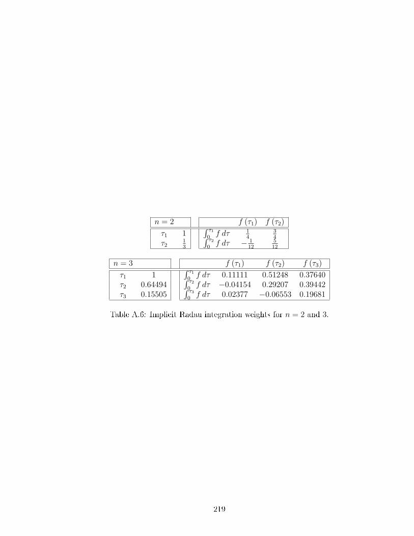
n = 2 f (τ1) f (τ2)
τ1 1∫ τ1
0f dτ 1
434
τ213
∫ τ20f dτ − 1
12512
n = 3 f (τ1) f (τ2) f (τ3)
τ1 1∫ τ1
0f dτ 0.11111 0.51248 0.37640
τ2 0.64494∫ τ2
0f dτ −0.04154 0.29207 0.39442
τ3 0.15505∫ τ3
0f dτ 0.02377 −0.06553 0.19681
Table A.6: Implicit Radau integration weights for n = 2 and 3.
219
APPENDIX B
Graveyard of Numbers
The arduous computer performs an amazing deed,
churning out myriads of numbers at dazzling speed.
Here lies an endless sea of numerical table,
Pages of pages one's mind couldn't fable.
220
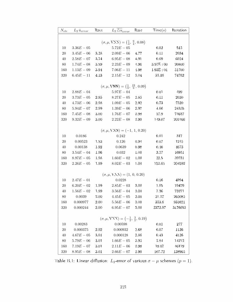
Nele L2 uerror Rate L24uerror Rate Time(s) Iteration
(σ, µ,VNN) =(
14 ,
94 , 0.08
)10 3.36E − 05 5.72E − 05 0.02 515
20 3.45E − 06 3.28 2.09E − 06 4.77 0.11 2034
40 2.58E − 07 3.74 6.95E − 08 4.91 0.69 6924
80 1.74E − 08 3.89 2.23E − 09 4.96 3.97E+00 20800
160 1.13E − 09 3.94 7.06E − 11 4.98 1.93E+01 51700
320 6.45E − 11 4.13 2.15E − 12 5.04 55.16 74762
(σ, µ,VNN) =(
19 ,
199 , 0.09
)10 2.88E − 04 5.97E − 04 0.01 499
20 3.73E − 05 2.95 8.27E − 05 2.85 0.11 2030
40 4.73E − 06 2.98 1.09E − 05 2.92 0.73 7320
80 5.94E − 07 2.99 1.39E − 06 2.97 4.66 24355
160 7.45E − 08 3.00 1.76E − 07 2.98 27.9 74637
320 9.32E − 09 3.00 2.22E − 08 2.99 149.07 202466
(σ, µ,VNN) = (−1, 1, 0.20)10 0.0186 0.242 0.01 317
20 0.00523 1.83 0.126 0.94 0.07 1245
40 0.00138 1.92 0.0639 0.98 0.46 4673
80 3.54E − 04 1.96 0.032 1.00 3.27 16951
160 8.97E − 05 1.98 1.60E − 02 1.00 22.5 59731
320 2.26E − 05 1.99 8.02E − 03 1.00 152.05 204592
(σ, µ,VNN) = (1, 0, 0.20)10 2.47E − 01 0.0228 0.16 4894
20 6.20E − 02 1.99 2.85E − 03 3.00 1.05 19479
40 1.56E − 02 1.99 3.56E − 04 3.00 7.36 73271
80 0.0039 2.00 4.45E − 05 3.00 51.27 265085
160 0.000977 2.00 5.56E − 06 3.00 353.6 931621
320 0.000244 2.00 6.95E − 07 3.00 2372.97 3176655
(σ, µ,VNN) =(− 1
2 ,32 , 0.19
)10 0.00283 0.00598 0.01 277
20 0.000375 2.92 0.000932 2.68 0.07 1126
40 4.67E − 05 3.01 0.000128 2.86 0.43 4126
80 5.79E − 06 3.01 1.66E − 05 2.95 2.84 14212
160 7.19E − 07 3.01 2.11E − 06 2.98 18.07 46119
320 8.95E − 08 3.01 2.66E − 07 2.99 107.72 138965
Table B.1: Linear diusion: L2-error of various σ − µ schemes (p = 1).
221

Nele L2 uerror Rate L24uerror Rate Time(s) Iteration
(σ, µ,VNN) = (0, 2, 0.10)10 0.000582 0.00113 0.02 46920 7.52E − 05 2.95 0.000163 2.79 0.1 190440 9.40E − 06 3.00 2.16E − 05 2.92 0.69 689480 1.17E − 06 3.01 2.78E − 06 2.96 4.43 23187160 1.46E − 07 3.00 3.52E − 07 2.98 27.03 72322320 1.82E − 08 3.00 4.43E − 08 2.99 149.84 202302
(σ, µ,VNN) = (0.0893, 2.5392, 0.08)10 0.00402 0.00143 0.02 60620 0.0013 1.63 0.000218 2.71 0.15 264040 0.000361 1.85 2.93E − 05 2.90 1.03 1027680 9.46E − 05 1.93 3.77E − 06 2.96 7.19 37473160 2.42E − 05 1.97 4.78E − 07 2.98 49.14 130970320 6.10E − 06 1.99 6.01E − 08 2.99 327.31 440358
(σ, µ,VNN) =(
16 ,
136 , 0.08
)10 0.000157 0.000367 0.02 540
20 2.05E − 05 2.94 4.82E − 05 2.93 0.11 2198
40 2.65E − 06 2.95 6.25E − 06 2.95 0.79 7875
80 3.38E − 07 2.97 7.97E − 07 2.97 4.98 26005
160 4.27E − 08 2.98 1.01E − 07 2.98 29.31 78417
320 5.36E − 09 2.99 1.27E − 08 2.99 151.56 205253
(σ, µ,VNN) = (−1, 3, 0.10)10 0.0126 0.00552 0.01 47520 0.00452 1.48 0.00092 2.58 0.12 219940 0.0013 1.80 0.000127 2.86 0.88 874380 0.000345 1.91 1.66E − 05 2.94 6.23 32344160 8.86E − 05 1.96 2.11E − 06 2.98 43.46 115168320 2.24E − 05 1.98 2.66E − 07 2.99 294.62 396262
(σ, µ,VNN) = (0, 3, 0.06)10 0.00535 0.00107 0.02 79520 0.00165 1.70 0.000161 2.73 0.19 349140 0.000449 1.88 2.16E − 05 2.90 1.36 1360780 0.000117 1.94 2.78E − 06 2.96 9.52 49637160 2.98E − 05 1.97 3.52E − 07 2.98 64.95 173359320 7.51E − 06 1.99 4.43E − 08 2.99 431.54 582031
Table B.2: Linear diusion: L2-error of various σ − µ schemes (p = 1).
222
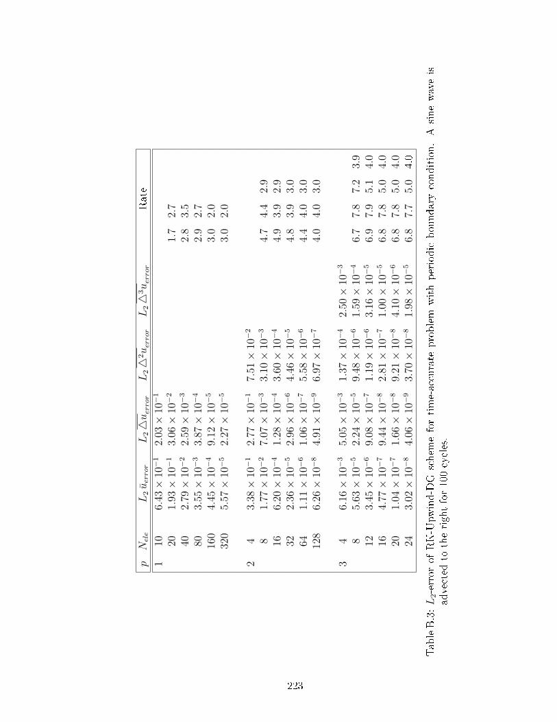
pNele
L2uerror
L24uerror
L24
2uerror
L24
3uerror
Rate
110
6.43×
10−
12.
03×
10−
1
201.
93×
10−
13.
06×
10−
21.
72.
740
2.79×
10−
22.
59×
10−
32.
83.
580
3.55×
10−
33.
87×
10−
42.
92.
716
04.
45×
10−
49.
12×
10−
53.
02.
032
05.
57×
10−
52.
27×
10−
53.
02.
0
24
3.38×
10−
12.
77×
10−
17.
51×
10−
2
81.
77×
10−
27.
07×
10−
33.
10×
10−
34.
74.
42.
916
6.20×
10−
41.
28×
10−
43.
60×
10−
44.
93.
92.
932
2.36×
10−
52.
96×
10−
64.
46×
10−
54.
83.
93.
064
1.11×
10−
61.
06×
10−
75.
58×
10−
64.
44.
03.
012
86.
26×
10−
84.
91×
10−
96.
97×
10−
74.
04.
03.
0
34
6.16×
10−
35.
05×
10−
31.
37×
10−
42.
50×
10−
3
85.
63×
10−
52.
24×
10−
59.
48×
10−
61.
59×
10−
46.
77.
87.
23.
912
3.45×
10−
69.
08×
10−
71.
19×
10−
63.
16×
10−
56.
97.
95.
14.
016
4.77×
10−
79.
44×
10−
82.
81×
10−
71.
00×
10−
56.
87.
85.
04.
020
1.04×
10−
71.
66×
10−
89.
21×
10−
84.
10×
10−
66.
87.
85.
04.
024
3.02×
10−
84.
06×
10−
93.
70×
10−
81.
98×
10−
56.
87.
75.
04.0
TableB.3:L
2-error
ofRK-Upwind-DG
schem
efortime-accurate
problem
withperiodic
boundarycondition.A
sinewaveis
advected
totherightfor100cycles.
223
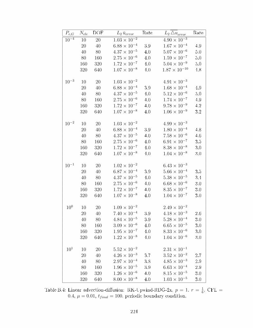
Pe,G Nele DOF L2 uerror Rate L24uerror Rate
10−4 10 20 1.03× 10⁻² 4.90× 10⁻³
20 40 6.88× 10⁻⁴ 3.9 1.67× 10⁻⁴ 4.940 80 4.37× 10⁻⁵ 4.0 5.07× 10⁻⁶ 5.080 160 2.75× 10⁻⁶ 4.0 1.59× 10⁻⁷ 5.0160 320 1.72× 10⁻⁷ 4.0 5.04× 10⁻⁹ 5.0320 640 1.07× 10⁻⁸ 4.0 1.87× 10⁻¹⁰ 4.8
10−3 10 20 1.03× 10⁻² 4.91× 10⁻³
20 40 6.88× 10⁻⁴ 3.9 1.68× 10⁻⁴ 4.940 80 4.37× 10⁻⁵ 4.0 5.12× 10⁻⁶ 5.080 160 2.75× 10⁻⁶ 4.0 1.74× 10⁻⁷ 4.9160 320 1.72× 10⁻⁷ 4.0 9.78× 10⁻⁹ 4.2320 640 1.07× 10⁻⁸ 4.0 1.06× 10⁻⁹ 3.2
10−2 10 20 1.03× 10⁻² 4.99× 10⁻³
20 40 6.88× 10⁻⁴ 3.9 1.80× 10⁻⁴ 4.840 80 4.37× 10⁻⁵ 4.0 7.58× 10⁻⁶ 4.680 160 2.75× 10⁻⁶ 4.0 6.91× 10⁻⁷ 3.5160 320 1.72× 10⁻⁷ 4.0 8.38× 10⁻⁸ 3.0320 640 1.07× 10⁻⁸ 4.0 1.04× 10⁻⁸ 3.0
10−1 10 20 1.02× 10⁻² 6.43× 10⁻³
20 40 6.87× 10⁻⁴ 3.9 5.66× 10⁻⁴ 3.540 80 4.37× 10⁻⁵ 4.0 5.38× 10⁻⁵ 3.480 160 2.75× 10⁻⁶ 4.0 6.68× 10⁻⁶ 3.0160 320 1.72× 10⁻⁷ 4.0 8.35× 10⁻⁷ 3.0320 640 1.07× 10⁻⁸ 4.0 1.04× 10⁻⁷ 3.0
100 10 20 1.09× 10⁻² 2.49× 10⁻²
20 40 7.40× 10⁻⁴ 3.9 4.18× 10⁻³ 2.640 80 4.84× 10⁻⁵ 3.9 5.28× 10⁻⁴ 3.080 160 3.09× 10⁻⁶ 4.0 6.65× 10⁻⁵ 3.0160 320 1.95× 10⁻⁷ 4.0 8.33× 10⁻⁶ 3.0320 640 1.22× 10⁻⁸ 4.0 1.04× 10⁻⁶ 3.0
101 10 20 5.52× 10⁻² 2.31× 10⁻¹
20 40 4.26× 10⁻³ 3.7 3.52× 10⁻² 2.740 80 2.97× 10⁻⁴ 3.8 4.85× 10⁻³ 2.980 160 1.96× 10⁻⁵ 3.9 6.63× 10⁻⁴ 2.9160 320 1.26× 10⁻⁶ 4.0 8.15× 10⁻⁵ 3.0320 640 8.00× 10⁻⁸ 4.0 1.03× 10⁻⁵ 3.0
Table B.4: Linear advection-diusion: RK-Upwind-RDG-2x, p = 1, r = 16, CFL =
0.4, µ = 0.01, tfinal = 100, periodic boundary condition.
224
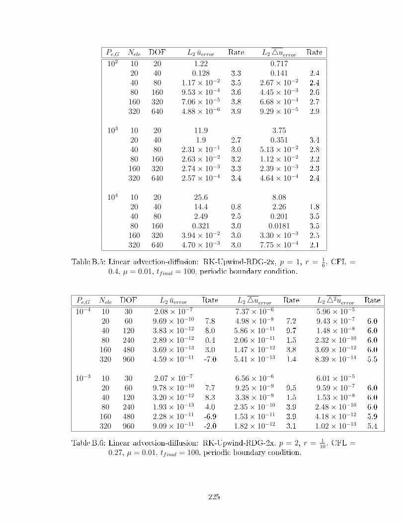
Pe,G Nele DOF L2 uerror Rate L24uerror Rate
102 10 20 1.22 0.71720 40 0.128 3.3 0.141 2.440 80 1.17× 10⁻² 3.5 2.67× 10⁻² 2.480 160 9.53× 10⁻⁴ 3.6 4.45× 10⁻³ 2.6160 320 7.06× 10⁻⁵ 3.8 6.68× 10⁻⁴ 2.7320 640 4.88× 10⁻⁶ 3.9 9.29× 10⁻⁵ 2.9
103 10 20 11.9 3.7520 40 1.9 2.7 0.351 3.440 80 2.31× 10⁻¹ 3.0 5.13× 10⁻² 2.880 160 2.63× 10⁻² 3.2 1.12× 10⁻² 2.2160 320 2.74× 10⁻³ 3.3 2.39× 10⁻³ 2.3320 640 2.57× 10⁻⁴ 3.4 4.64× 10⁻⁴ 2.4
104 10 20 25.6 8.0820 40 14.4 0.8 2.26 1.840 80 2.49 2.5 0.201 3.580 160 0.321 3.0 0.0181 3.5160 320 3.94× 10⁻² 3.0 3.30× 10⁻³ 2.5320 640 4.70× 10⁻³ 3.0 7.75× 10⁻⁴ 2.1
Table B.5: Linear advection-diusion: RK-Upwind-RDG-2x, p = 1, r = 16, CFL =
0.4, µ = 0.01, tfinal = 100, periodic boundary condition.
Pe,G Nele DOF L2 uerror Rate L24uerror Rate L242uerror Rate
10−4 10 30 2.08× 10⁻⁷ 7.37× 10⁻⁶ 5.96× 10⁻⁵
20 60 9.69× 10⁻¹⁰ 7.8 4.98× 10⁻⁸ 7.2 9.43× 10⁻⁷ 6.040 120 3.83× 10⁻¹² 8.0 5.86× 10⁻¹¹ 9.7 1.48× 10⁻⁸ 6.080 240 2.89× 10⁻¹² 0.4 2.06× 10⁻¹¹ 1.5 2.32× 10⁻¹⁰ 6.0160 480 3.69× 10⁻¹³ 3.0 1.47× 10⁻¹² 3.8 3.69× 10⁻¹² 6.0320 960 4.59× 10⁻¹¹ -7.0 5.41× 10⁻¹³ 1.4 8.39× 10⁻¹⁴ 5.5
10−3 10 30 2.07× 10⁻⁷ 6.56× 10⁻⁶ 6.01× 10⁻⁵
20 60 9.78× 10⁻¹⁰ 7.7 9.25× 10⁻⁹ 9.5 9.59× 10⁻⁷ 6.040 120 3.20× 10⁻¹² 8.3 3.38× 10⁻⁹ 1.5 1.53× 10⁻⁸ 6.080 240 1.93× 10⁻¹³ 4.0 2.35× 10⁻¹⁰ 3.9 2.48× 10⁻¹⁰ 6.0160 480 2.28× 10⁻¹¹ -6.9 1.53× 10⁻¹¹ 3.9 4.18× 10⁻¹² 5.9320 960 9.09× 10⁻¹¹ -2.0 1.82× 10⁻¹² 3.1 1.02× 10⁻¹³ 5.4
Table B.6: Linear advection-diusion: RK-Upwind-RDG-2x, p = 2, r = 110, CFL =
0.27, µ = 0.01, tfinal = 100, periodic boundary condition.
225

pNele
L2uerror
L24uerror
L24
2uerror
L24
3uerror
Rate
16
5.51×
10−
33.
19×
10−
3
121.
35×
10−
34.
26×
10−
42.
02.
918
5.99×
10−
41.
29×
10−
42.
02.
924
3.37×
10−
45.
52×
10−
52.
02.
930
2.15×
10−
42.
85×
10−
52.
02.
936
1.50×
10−
41.
66×
10−
51.
92.
9
24
1.45×
10−
31.
38×
10−
31.
77×
10−
3
85.
51×
10−
42.
08×
10−
41.
76×
10−
41.
42.
73.
312
2.69×
10−
46.
43×
10−
54.
38×
10−
51.
72.
93.
416
1.57×
10−
42.
76×
10−
51.
62×
10−
51.
82.
93.
420
1.02×
10−
41.
42×
10−
57.
50×
10−
61.
92.
93.
424
7.19×
10−
58.
27×
10−
63.
98×
10−
61.
92.
93.
4
34
5.64×
10−
51.
53×
10−
51.
43×
10−
45.
13×
10−
5
61.
24×
10−
51.
75×
10−
63.
02×
10−
56.
17×
10−
63.
75.
33.
85.
28
4.07×
10−
63.
68×
10−
79.
75×
10−
61.
38×
10−
63.
85.
43.
95.
210
1.69×
10−
61.
09×
10−
74.
03×
10−
64.
31×
10−
73.
95.
43.
95.
212
8.25×
10−
74.
02×
10−
81.
95×
10−
61.
68×
10−
73.
95.
43.
95.
114
4.48×
10−
71.
73×
10−
81.
06×
10−
67.
56×
10−
83.
95.
43.
95.
1
TableB.7:RDG-1x-Naive,VNN=0.07,0.02,and0.01
forRK3,RK4,andRK5,respectively:L
2-error
ofsteadylinear-variation
diusion
problem
withtwo-sided
Neumannboundaryconditions.
226
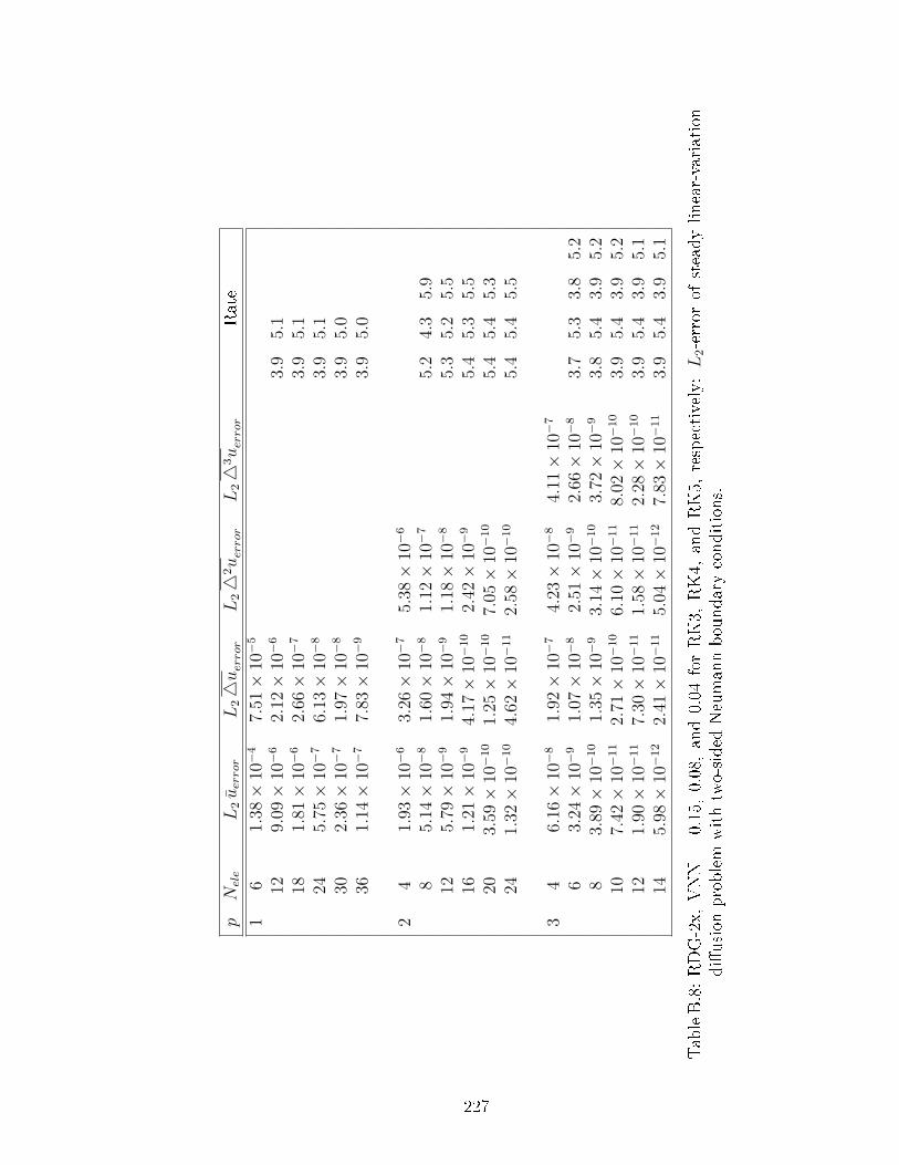
pNele
L2uerror
L24uerror
L24
2uerror
L24
3uerror
Rate
16
1.38×
10−
47.
51×
10−
5
129.
09×
10−
62.
12×
10−
63.
95.
118
1.81×
10−
62.
66×
10−
73.
95.
124
5.75×
10−
76.
13×
10−
83.
95.
130
2.36×
10−
71.
97×
10−
83.
95.
036
1.14×
10−
77.
83×
10−
93.
95.
0
24
1.93×
10−
63.
26×
10−
75.
38×
10−
6
85.
14×
10−
81.
60×
10−
81.
12×
10−
75.
24.
35.
912
5.79×
10−
91.
94×
10−
91.
18×
10−
85.
35.
25.
516
1.21×
10−
94.
17×
10−
10
2.42×
10−
95.
45.
35.
520
3.59×
10−
10
1.25×
10−
10
7.05×
10−
10
5.4
5.4
5.3
241.
32×
10−
10
4.62×
10−
11
2.58×
10−
10
5.4
5.4
5.5
34
6.16×
10−
81.
92×
10−
74.
23×
10−
84.
11×
10−
7
63.
24×
10−
91.
07×
10−
82.
51×
10−
92.
66×
10−
83.
75.
33.
85.
28
3.89×
10−
10
1.35×
10−
93.
14×
10−
10
3.72×
10−
93.
85.
43.
95.
210
7.42×
10−
11
2.71×
10−
10
6.10×
10−
11
8.02×
10−
10
3.9
5.4
3.9
5.2
121.
90×
10−
11
7.30×
10−
11
1.58×
10−
11
2.28×
10−
10
3.9
5.4
3.9
5.1
145.
98×
10−
12
2.41×
10−
11
5.04×
10−
12
7.83×
10−
11
3.9
5.4
3.9
5.1
TableB.8:RDG-2x,VNN
=0.15,0.08,and0.04
forRK3,
RK4,
andRK5,
respectively:L
2-error
ofsteadylinear-variation
diusion
problem
withtwo-sided
Neumannboundaryconditions.
227
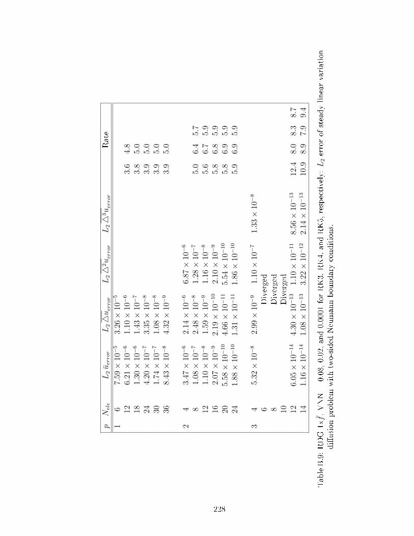
pNele
L2uerror
L24uerror
L24
2uerror
L24
3uerror
Rate
16
7.59×
10−
53.
26×
10−
5
126.
21×
10−
61.
10×
10−
63.
64.
818
1.30×
10−
61.
43×
10−
73.
85.
024
4.20×
10−
73.
35×
10−
83.
95.
030
1.74×
10−
71.
08×
10−
83.
95.
036
8.43×
10−
84.
32×
10−
93.
95.
0
24
3.47×
10−
62.
14×
10−
66.
87×
10−
6
81.
08×
10−
72.
48×
10−
81.
28×
10−
75.
06.
45.
712
1.10×
10−
81.
59×
10−
91.
16×
10−
85.
66.
75.
916
2.07×
10−
92.
19×
10−
10
2.10×
10−
95.
86.
85.
920
5.58×
10−
10
4.66×
10−
11
5.54×
10−
10
5.8
6.9
5.9
241.
88×
10−
10
1.31×
10−
11
1.86×
10−
10
5.9
6.9
5.9
34
5.32×
10−
82.
99×
10−
91.
10×
10−
71.
33×
10−
8
6Diverged
8Diverged
10Diverged
126.
05×
10−
14
4.30×
10−
13
1.10×
10−
11
8.56×
10−
13
12.4
8.0
8.3
8.7
141.
16×
10−
14
1.08×
10−
13
3.22×
10−
12
2.14×
10−
13
10.9
8.9
7.9
9.4
TableB.9:RDG-1xf,VNN=
0.08,0.02,and0.0001
forRK3,
RK4,
andRK5,
respectively:L
2-error
ofsteadylinear-variation
diusion
problem
withtwo-sided
Neumannboundaryconditions.
228
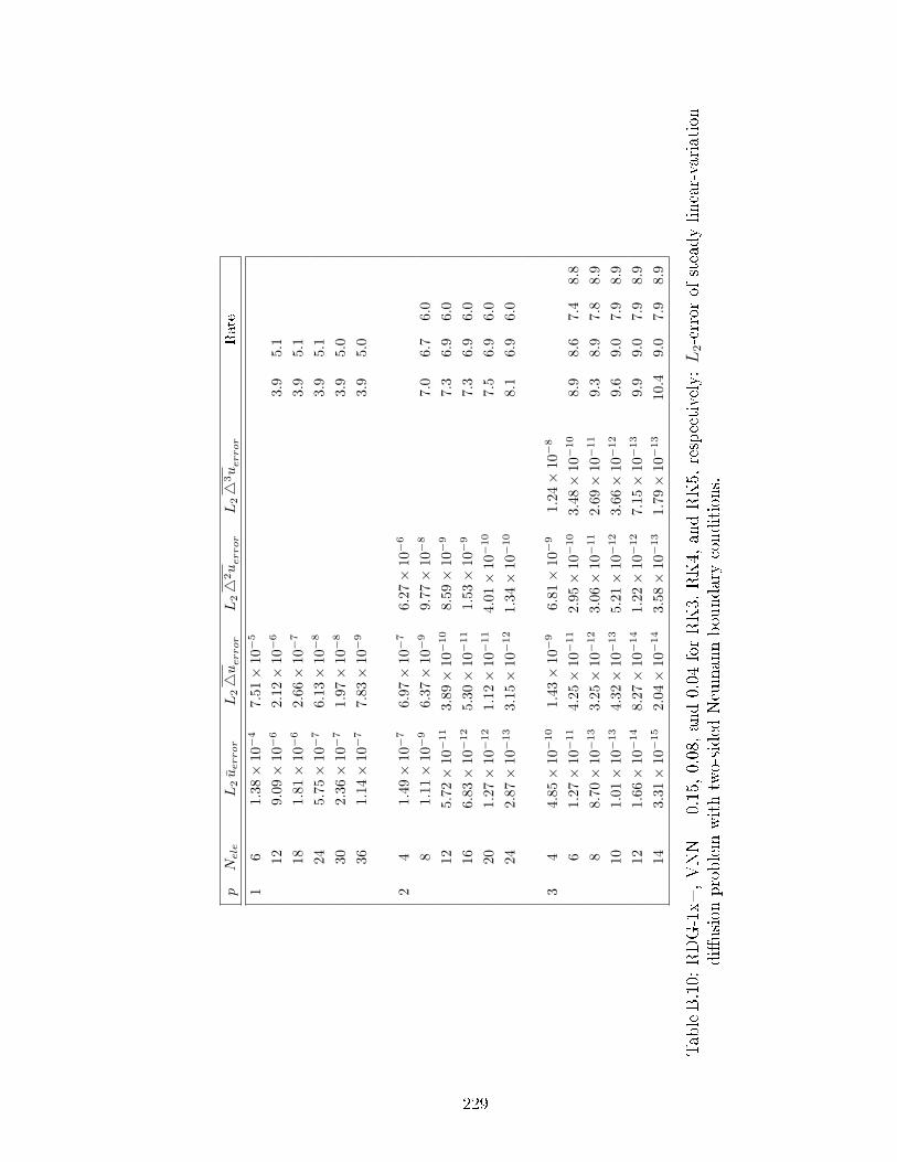
pN
ele
L2u
error
L24u
error
L24
2u
error
L24
3u
error
Rate
16
1.38×
10−
47.
51×
10−
5
129.
09×
10−
62.
12×
10−
63.
95.
118
1.81×
10−
62.
66×
10−
73.
95.
124
5.75×
10−
76.
13×
10−
83.
95.
130
2.36×
10−
71.
97×
10−
83.
95.
036
1.14×
10−
77.
83×
10−
93.
95.
0
24
1.49×
10−
76.
97×
10−
76.
27×
10−
6
81.
11×
10−
96.
37×
10−
99.
77×
10−
87.
06.
76.
012
5.72×
10−
11
3.89×
10−
10
8.59×
10−
97.
36.
96.
016
6.83×
10−
12
5.30×
10−
11
1.53×
10−
97.
36.
96.
020
1.27×
10−
12
1.12×
10−
11
4.01×
10−
10
7.5
6.9
6.0
242.
87×
10−
13
3.15×
10−
12
1.34×
10−
10
8.1
6.9
6.0
34
4.85×
10−
10
1.43×
10−
96.
81×
10−
91.
24×
10−
8
61.
27×
10−
11
4.25×
10−
11
2.95×
10−
10
3.48×
10−
10
8.9
8.6
7.4
8.8
88.
70×
10−
13
3.25×
10−
12
3.06×
10−
11
2.69×
10−
11
9.3
8.9
7.8
8.9
101.
01×
10−
13
4.32×
10−
13
5.21×
10−
12
3.66×
10−
12
9.6
9.0
7.9
8.9
121.
66×
10−
14
8.27×
10−
14
1.22×
10−
12
7.15×
10−
13
9.9
9.0
7.9
8.9
143.
31×
10−
15
2.04×
10−
14
3.58×
10−
13
1.79×
10−
13
10.4
9.0
7.9
8.9
TableB.10:
RDG-1x+,VNN
=0.15,0.08,and0.04
forRK3,
RK4,
andRK5,
respectively:L
2-error
ofsteadylinear-variation
diusion
problem
withtwo-sided
Neumannboundaryconditions.
229

Pe,G Nele DOF L2 uerror OOA L24uerror OOA
10−5 10 20 6.59× 10⁻⁵ 3.68× 10⁻⁵
20 40 4.13× 10⁻⁶ 4.0 1.17× 10⁻⁶ 4.9
40 80 2.59× 10⁻⁷ 4.0 3.66× 10⁻⁸ 5.0
80 160 1.62× 10⁻⁸ 4.0 1.15× 10⁻⁹ 5.0
160 320 1.01× 10⁻⁹ 4.0 4.11× 10⁻¹¹ 4.8
320 640 6.34× 10⁻¹¹ 4.0 1.81× 10⁻¹² 4.5
10−4 10 20 6.59× 10⁻⁵ 3.68× 10⁻⁵
20 40 4.13× 10⁻⁶ 4.0 1.18× 10⁻⁶ 5.0
40 80 2.59× 10⁻⁷ 4.0 3.77× 10⁻⁸ 5.0
80 160 1.62× 10⁻⁸ 4.0 1.47× 10⁻⁹ 4.7
160 320 1.01× 10⁻⁹ 4.0 2.02× 10⁻¹⁰ 2.9
320 640 6.33× 10⁻¹¹ 4.0 1.42× 10⁻¹¹ 3.8
10−3 10 20 6.58× 10⁻⁵ 3.81× 10⁻⁵
20 40 4.13× 10⁻⁶ 4.0 1.54× 10⁻⁶ 4.6
40 80 2.59× 10⁻⁷ 4.0 8.62× 10⁻⁸ 4.2
80 160 1.62× 10⁻⁸ 4.0 9.10× 10⁻⁹ 3.2
160 320 1.01× 10⁻⁹ 4.0 1.97× 10⁻⁹ 2.2
320 640 6.33× 10⁻¹¹ 4.0 1.41× 10⁻¹⁰ 3.8
10−2 10 20 6.53× 10⁻⁵ 7.35× 10⁻⁵
20 40 4.13× 10⁻⁶ 4.0 9.45× 10⁻⁶ 3.0
40 80 2.59× 10⁻⁷ 4.0 7.60× 10⁻⁷ 3.6
80 160 1.62× 10⁻⁸ 4.0 9.08× 10⁻⁸ 3.0
160 320 1.01× 10⁻⁹ 4.0 1.80× 10⁻⁸ 2.3
320 640 6.35× 10⁻¹¹ 4.0 1.42× 10⁻⁹ 3.7
10−1 10 20 8.43× 10⁻⁵ 3.54× 10⁻⁴
20 40 6.74× 10⁻⁶ 3.6 9.98× 10⁻⁵ 2.4
40 80 3.24× 10⁻⁷ 4.4 7.01× 10⁻⁶ 3.8
80 160 2.30× 10⁻⁸ 3.8 1.17× 10⁻⁶ 2.6
160 320 1.29× 10⁻⁹ 4.2 1.13× 10⁻⁷ 3.4
320 640 8.57× 10⁻¹¹ 3.9 1.62× 10⁻⁸ 2.8
100 10 20 2.94× 10⁻⁴ 2.34× 10⁻³
20 40 2.53× 10⁻⁵ 3.6 4.19× 10⁻⁴ 2.5
40 80 1.78× 10⁻⁶ 3.8 5.88× 10⁻⁵ 2.8
80 160 1.42× 10⁻⁷ 3.7 9.57× 10⁻⁶ 2.6
160 320 8.20× 10⁻⁹ 4.1 1.08× 10⁻⁶ 3.2
320 640 8.72× 10⁻¹⁰ 3.2 2.46× 10⁻⁷ 2.1
Table B.11: Linear advection-diusion: HH-DG p = 1, r = 16, CFL = 1, µ = 0.01,
tfinal = 100, CAdv-Di = 0.9375, periodic boundary condition.
230

Pe,G Nele DOF L2 uerror OOA L24uerror OOA
10+1 10 20 1.48× 10⁻³ 7.69× 10⁻³
20 40 1.70× 10⁻⁴ 3.1 1.34× 10⁻³ 2.5
40 80 1.98× 10⁻⁵ 3.1 3.25× 10⁻⁴ 2.0
80 160 2.01× 10⁻⁶ 3.3 6.92× 10⁻⁵ 2.2
160 320 1.64× 10⁻⁷ 3.6 8.02× 10⁻⁶ 3.1
320 640 1.40× 10⁻⁸ 3.5 2.11× 10⁻⁶ 1.9
10+2 10 20 6.57× 10⁻³ 5.57× 10⁻³
20 40 9.77× 10⁻⁴ 2.8 1.51× 10⁻³ 1.9
40 80 1.49× 10⁻⁴ 2.7 2.91× 10⁻⁴ 2.4
80 160 2.21× 10⁻⁵ 2.8 8.07× 10⁻⁵ 1.9
160 320 3.00× 10⁻⁶ 2.9 1.72× 10⁻⁵ 2.2
320 640 3.60× 10⁻⁷ 3.1 7.01× 10⁻⁶ 1.3
10+3 10 20 2.27× 10⁻² 7.48× 10⁻³
20 40 4.35× 10⁻³ 2.4 1.34× 10⁻³ 2.5
40 80 7.53× 10⁻⁴ 2.5 3.05× 10⁻⁴ 2.1
80 160 1.19× 10⁻⁴ 2.7 8.55× 10⁻⁵ 1.8
160 320 1.79× 10⁻⁵ 2.7 2.52× 10⁻⁵ 1.8
320 640 2.71× 10⁻⁶ 2.7 4.39× 10⁻⁶ 2.5
10+4 10 20 8.18× 10⁻³ 2.50× 10⁻²
20 40 1.48× 10⁻³ 2.5 2.43× 10⁻³ 3.4
40 80 2.46× 10⁻³ 2.6 3.93× 10⁻⁴ 2.6
80 160 4.29× 10⁻⁴ 2.5 2.25× 10⁻⁵ 4.3
160 320 7.68× 10⁻⁵ 2.5 1.44× 10⁻⁵ 0.6
320 640 1.34× 10⁻⁵ 2.5 5.01× 10⁻⁶ 1.5
10+5 10 20 2.46× 10⁻¹ 7.79× 10⁻²
20 40 8.89× 10⁻² 1.5 1.41× 10⁻² 2.5
40 80 1.40× 10⁻² 2.7 1.14× 10⁻³ 3.6
80 160 1.95× 10⁻³ 2.8 1.20× 10⁻⁴ 3.3
160 320 2.83× 10⁻⁴ 2.8 1.78× 10⁻⁵ 2.8
320 640 0.00× 10⁻¹¹ 0.0 0.00× 10⁻⁸ 0.0
Table B.12: Linear advection-diusion: HH-DG p = 1, r = 16, CFL = 1, µ = 0.01,
tfinal = 100, CAdv-Di = 0.9375, periodic boundary condition.
231

BIBLIOGRAPHY
232

BIBLIOGRAPHY
[1] Saint Petersburg State Polytechnical University. http://smitu.cef.spbstu.
ru/galerkin.htm.
[2] D.N. Arnold. An interior penalty nite element method with discontinuouselements. SIAM Journal on Numerical Analysis, 19:742760, 1982.
[3] D.N. Arnold, F. Brezzi, B. Cockburn, and L.D. Marini. Unied analysis of dis-continuous galerkin methods for elliptic problems. SIAM Journal on NumericalAnalysis, 39:17491779, 2002.
[4] F. Bassi and S. Rebay. A high-order accurate discontinuous nite elementmethod for the numerical solution of the compressible navier-stokes equations.Journal of Computational Physics, 131:267279, 1997.
[5] C.E. Baumann and J.T. Oden. A discontinuous hp nite element method forconvection-diusion problems. Computer Methods in Applied Mechanics andEngineering, 175:311341, 1999.
[6] B. Cockburn, J. Gopalakrishnan, and R. Lazarov. Unied hybridization of dis-continuous Galerkin, mixed, and continuous Galerkin methods for second orderelliptic problems. Siam, Journal on Numerical Analysis, 47:13191365, 2009.
[7] B. Cockburn and C.W. Shu. TVB Runge-Kutta local projection discontinuousGalerkin nite element method for conservation laws II: General framework.Mathematics of Computation, 52:411435, 1989.
[8] B. Cockburn and C.W. Shu. The local discontinuous Galerkin method for time-dependent convection-diusion systems. Siam, Journal on Numerical Analysis,35:24402463, 1998.
[9] L.M. Delves and C.A. Hall. An implicit matching principle for global elementcalculations. Institute of Mathematics and its Applications, 23:223234, 1979.
[10] M. Dumbser and C-D. Munz. ADER discontinuous Galerkin schemes for aeroa-coustics. C.R. Mecanique 333, pages 683687, 2005.
[11] B. Finlayson. The method of weighted residuals and variational principle, withapplication in uid mechanics. Academic Press, 1972.
233
[12] D. French, M.C. Galbraith, and M. Osorio. Error analysis of a modied discon-tinuous Galerkin recovery scheme for diusion problems. 48th AIAA AerospaceSiciences Meeting including the New Horizons Forum and Aerospace Exposition,AIAA Paper 2010-1071, 2010.
[13] J.E. Fromm. A method for reducing dispersion in convective dierence schemes.Journal of Computational Physics, 3:176189, 1968.
[14] G. Gassner, F. Lorcher, and C.D. Munz. A contribution to the construction ofdiusion uxes for nite volume and discontinuous Galerkin schemes. Journalof Scientic Computational Physics, 224:10491063, 2007.
[15] G. Gassner, F. Lorcher, and C.D. Munz. A discontinuous Galkerin schemebased on a space-time expansion. II. viscous ow equations in multi dimensions.Journal of Scientic Computing, 34:260286, 2008.
[16] S. Gottlieb. On high order strong stability preserving Runge-Kutta and multistep time discretizations. Journal of Scientic Computing, 25:105128, 2005.
[17] H.T. Huynh. An upwind moment scheme for conservation laws. Computa-tional Fluid Dynamics 2004, Proceedings of the Third International Conferenceon Computational Fluid Dynamics, ICCFD3, Toronto, pages 761766, 2006.
[18] H.T. Huynh. A ux reconstruction approach to high-order schemes includingdiscontinuous Galkerin methods. 18th AIAA Computational Fluid DynamicsConference, 2007.
[19] H.T. Huynh. A reconstruction approach to high-order schemes including discon-tinuous Galerkin for diusion. 47th AIAA Aerospace Sciences Meeting IncludingThe New Horizons Forum and Aerospace Exposition, AIAA Paper 2009-0403,2009.
[20] A. Jameson, W. Schmidt, and E. Turkel. Numerical solution of the Eulerequations by nite volume methods using Runge-Kutta time-stepping schemes.AIAA Fluid and Plasma Dynamics Conference, 14th, Palo Alto, CA, USA,AIAA Paper 81-1259, 1981.
[21] C. Johnson and J. Pitkaranta. An analysis of the discontinuous Galerkin methodfor a scalar hyperbolic equation. Mathematics of Computation, 46:126, 1986.
[22] P. LeSaint and P.A. Raviart. On a nite element method for solving the neu-tron transport equation. Mathmetical Aspects of Finite Elements in PartialDierential Equations, pages 89123, 1974.
[23] M. Lo and B. van Leer. Analysis and implementation of Recovery-based Dis-continuous Galerkin for diusion. 19th AIAA Computational Fluid DynamicsConference, San Antonio, Texas, USA, AIAA Paper 2009-3786, 2009.
234
[24] F. Lorcher, G. Gassner, and C.D. Munz. A discontinuous Galkerin scheme basedon a space-time expansion. I. inviscid compressible ow in one space dimension.Journal of Scientic Computating, 32:175199, 2007.
[25] K. Masatsuka. I do like CFD, Vol. 1. Lulu.com, 2009.
[26] K.W. Morton. Shock capturing, tting and recovery. SpringerBerlin/Heidelberg, 1982.
[27] N.C. Nguyen, J. Peraire, and B. Cockburn. An implicit high-order hybridiz-able discontinuous Galerkin method for linear convection-diusion equations.Journal of Computational Physics, 228:32323254, 2009.
[28] J.T. Oden, I. Babuska, and C.E. Baumann. A discontinuous hp nite elementmethod for diusion problems. Journal of Computational Physics, 146:491519,1998.
[29] H. Park, R. Nourgaliev, V. Mousseau, and D. Knoll. Recovery discontinu-ous Galerkin - Jacobian-free Newton Krylov (rDG-JFNK) method for all-speedNavier-Stokes equations. International Conference on Computational Fluid Dy-namics (ICCFD), Seoul, Korea, 2008.
[30] J. Peraire and P.O. Persson. The compact discontinuous galerkin (CDG)method for elliptic problems. SIAM Journal of Scientic Computating, 30:18061824, 2008.
[31] M. J. Prather. Numerical advection by conservation of second-order moments.JGR, 91:66716681, 1986.
[32] W. Reed and T. Hill. Triangular mesh methods for the neutron transportequation. Tech. Rep. LA-UR 73-479, Los Alamos National Laboratory, 1973.
[33] P.L. Roe. Approximate Riemann solvers, parameter vectors, and dierenceschemes. Journal of Computational Physics, 43(2):357 372, 1981.
[34] G.L. Russel and J.A. Lerner. A new nite-dierencing scheme for the tracertransport equation. Journal of Applied Meteorology, 20:14831498, 1981.
[35] S.J. Ruuth. Global optimization of explicit strong-stability-preserving Runge-Kutta methods. Mathematics of Computation, 75:183207, 1997.
[36] Y. Suzuki. Discontinuous Galerkin Methods for Extended Hydrodynamics.PhD Thesis, 2008.
[37] B. van Leer. Towards the ultimate conservative dierence scheme. IV. A newapproach to numerical convection. Journal of Computational Physics, 23:276299, 1977.
235
[38] B. van Leer. Towards the ultimate conservative dierence scheme. V. A second-order sequel to Godunov's method. Journal of Computational Physics, 32:101136, 1979.
[39] B. van Leer. Computational methods for ideal compressible ow. In VonKarman Inst. for Fluid Dynamics Computational Fluid Dyn., 1:45, 1984.
[40] B. van Leer. Multidimensional explicit dierence schemes for hyperbolic con-servation laws. Computational Methods in Applied Sciences and Engineering,VI, pages 493497, 1984.
[41] B. van Leer and M. Lo. Unication of Discontinuous Galerkin methods foradvection and diusion. 47th AIAA Aerospace Sciences Meeting and Exhibit,Orlando, Florida, USA, AIAA Paper 2009-400, 2009.
[42] B. van Leer, M. Lo, R. Gitik, and S. Nomura. A Venerable Family of Dis-continuous Galerkin Schemes for Diusion Revisited. World Scientic ReviewVolume 9, 2010.
[43] B. van Leer, M. Lo, and M. van Raalte. A discontinuous Galerkin methodfor diusion based on recovery. 18th AIAA Computational Fluid DynamicsConference, Miami, Florida, USA, AIAA Paper 2007-4083, June 2007.
[44] B. van Leer and S. Nomura. Discontinuous Galerkin for diusion. 17th AIAAComputational Fluid Dynamics Conference, Tornoto, Ontario, Canada, AIAAPaper 2005-5108, 2005.
[45] M. van Raalte and B. van Leer. Bilinear forms for the Recovery-based Dis-continuous Galerkin method for diusion. Communications in ComputationalPhysics, 5:683693, 2008.
[46] F.M. White. Viscous Fluid Flow, Second Edition. McGraw-Hill, 1991.
[47] Wikipedia. http://en.wikipedia.org/wiki/Runge_Kutta_methods.
236