energies

Article

A Smart Forecasting Approach to DistrictEnergy Management

Baris Yuce 1,2,*,†, Monjur Mourshed 1,* ID and Yacine Rezgui 1

1 BRE Trust Centre for Sustainable Engineering, School of Engineering, Cardiff University,Cardiff CF24 3AA, UK; RezguiY@cardiff.ac.uk

2 College of Engineering, Mathematics, and Physical Sciences, School of Engineering,Streatham Campus University of Exeter, Exeter EX4 4QJ, UK

* Correspondence: B.Yuce@exeter.ac.uk (B.Y.); MourshedM@cardiff.ac.uk (M.M.);Tel.: +44-13-972-4562 (B.Y.); +44-29-2087-4847 (M.M.)

† The research reported in this study was conducted while Baris Yuce was affiliated with Cardiff University.

Academic Editor: Joseph H. M. TahReceived: 15 May 2017; Accepted: 14 July 2017; Published: 25 July 2017

Abstract: This study presents a model for district-level electricity demand forecasting using a setof Artificial Neural Networks (ANNs) (parallel ANNs) based on current energy loads and socialparameters such as occupancy. A comprehensive sensitivity analysis is conducted to select theinputs of the ANN by considering external weather conditions, occupancy type, main incomeproviders’ employment status and related variables for the fuel poverty index. Moreover, a detailedparameter tuning is conducted using various configurations for each individual ANN. The studyalso demonstrates the strength of the parallel ANN models in different seasons of the years. Inthe proposed district level energy forecasting model, the training and testing stages of parallelANNs utilise dataset of a group of six buildings. The aim of each individual ANN is to predictelectricity consumption and the aggregated demand in sub-hourly time-steps. The inputs of eachANN are determined using Principal Component Analysis (PCA) and Multiple Regression Analysis(MRA) methods. The accuracy and consistency of ANN predictions are evaluated using Pearsoncoefficient and average percentage error, and against four seasons: winter, spring, summer, andautumn. The lowest prediction error for the aggregated demand is about 4.51% for winter season andthe largest prediction error is found as 8.82% for spring season. The results demonstrate that peakdemand can be predicted successfully, and utilised to forecast and provide demand-side flexibility tothe aggregators for effective management of district energy systems.

Keywords: ANN; PCA; MRA; district energy management; smart grid; smart cities; demandforecasting

1. Introduction

Sustainable generation and supply of energy has become one of the biggest challenges facedby policy makers, scientists, and researchers [1], primarily because of both an increase in energydemand and the technological (infrastructure) improvements required to respond effectively tothis growth in demand. In fact, the average electricity demand increased by about 37% between1990 and 2008 in the European Union (27 EU countries) [2]. Hence, there is a need for concertedinnovative strategies to tackle this increasing demand, estimated at 1.4% per annum [3], througheffective energy policies. Moreover, EU heads of states and governments set three targets in2007 to be met by 2020: (i) reduction of greenhouse gas emissions by at least 20% compared to1990 levels; (ii) increase of the share of renewable energy to 20% of EU energy consumption; and(iii) reduction of primary energy usage by 20% through improved energy efficiency [2]. To achieve

Energies 2017, 10, 1073; doi:10.3390/en10081073 www.mdpi.com/journal/energies

Energies 2017, 10, 1073 2 of 22

these targets, the European Commission (EC) has initiated the European Strategic Energy TechnologyPlan (SET-Plan), aimed at accelerating the development and deployment of low-carbon technologiesfor transforming the European energy system to implement the fifth pillar of the Energy Union [4].Further, the SET-Plan recommends the optimisation of the current energy- and electricity-grid withfederation-based approaches focusing on decentralised micro-grids [4]. While new decentralisedmicro-grids are required to be part of the low-and-medium-voltage (LV/MV) electricity grids [5,6],the centralised and federation-based grid management approach offers an efficient control of theentire electricity grid [7]. Traditional electricity grids are static systems; they do not provide detailedinformation about energy consumption on the demand side, making it difficult to address peakconsumptions [8]. Moreover, both consumer behaviour and electricity markets are evolving rapidly,progressing towards a user-centric direction—transforming the centralised, uni-directional traditionalgrid into a decentralised energy-sharing grid with a bi-directional flow of information and energy [6].This change creates a new form of end users termed “prosumers”, who are both energy producerswithin their micro-grid (renewable sources such as photovoltaic (PV) and wind, and combined heatand power (CHP) technologies) and energy consumers [9–11]. Prosumers add complexity to themanagement of the entire electricity grid, requiring advanced distributed solutions rather thantraditional approaches of centralised energy management [6]. With the Feed-in-tariffs (FiT), prosumersprefer to maximise their gain from micro electricity grids.

Several smart district energy management models have been proposed in the literature to maximisebenefits for the entire grid [12–18]. Fonseca et al. [12] proposed an integrated framework to maximisethe utility of the micro-grid concept in the district level. Fanti et al. [13] proposed a district energymanagement model to optimise the smart grid with a linear programming approach and to predictnegotiated results for the next day’s energy consumption and relevant cost, with a view to reducing thetotal cost for the entire district. Van Pruissen et al. [14] compared the efficiency of a multi-agent basedenergy market management system to traditional systems, and illustrated the benefits of the multi-agentbased solutions. One of the main problems to be tackled during the optimisation and control of suchlarge-scale systems is the prediction of loads. The optimisation and the determination of flexibilityin district and urban level electricity-grids suffer from a lack of detailed (temporally and spatially)and prior knowledge about demand profiles [15,16]. Hence, Jing et al. [17] proposed a forecastingmodel for district energy management using empirical models alongside an optimisation system toreduce energy costs. However, empirical models require certain assumptions, which increase modelcomplexity. Further, district energy consumption has an uncertain energy consumption pattern, whichmeans that demand for the energy consumption may fluctuate during the days of years or hours of thedays. These fluctuations are mostly related to the seasonal effects and socio-economic factors such asoccupants’ behaviour and the changes in their economic circumstances. In addition, the existence offuel poverty at the household level affects energy demand which needs to be considered for districtlevel forecasting. Many households fail to ensure a warm home, especially during cold winter days,because of low incomes, thermally inefficient homes and high energy prices [18,19]. To deal with thesetypes of complexities, advanced, adaptive and intelligent solutions are often required. Related smartsolutions provide promising means in the built environment to control and predict energy consumption.These include artificial neural network [11,20], support vector machine [21], genetic algorithm [22], andrule- [23], and ontology-based systems [24]. They have also been utilised in district energy managementproblems. Powell et al. [15] proposed an ANN-based forecasting system prior to the optimisation andcontrol of the district-level energy grid, as well as large-scale systems.

Load forecasting using machine learning (ML) algorithms has become very popular because ofthe increasing need for cost-effective prediction of demand at a finer temporal resolution to operateand manage the grid in cost- and energy-efficient manner. Several studies have proposed variousapproaches for ML-based prediction. Kandananound [25] presented a forecasting process in Thailandto predict the electricity demand using three approaches: Autoregressive Integrated Moving Average(ARIMA) method, ANN and Multiple Linear Regression (MLR) on the annual electricity consumption

Energies 2017, 10, 1073 3 of 22

data (1986–2010). ANN-based approach performed better than the remaining two in the study.Hernandez et al. [26] proposed an ANN-based load forecasting system to predict hourly basedenergy generation data using solar radiation information. They have found that the disaggregatedload forecasting increased the complexity of predicting electricity load for the next hour. Their bestperformed ANN predicted short-term electricity load with 15.34% Mean Absolute Percentage Error(MAPE). Similarly, Srinivasan [27] proposed an evolved ANN based forecasting system to predict theweekdays and weekends electric loads using Genetic Algorithm (GA) as the optimisation engine. Theproposed model forecasts hourly electricity load. The results indicate that the ANN-GA predicts theload better than the statistical approaches. However, this model utilises average hourly based electricityload where the average energy consumption may differ from the actual hourly based load. Further, thestudy does not demonstrate individual consumers’ demand (building level electricity consumption);hence, the proposed ANN-GA based forecasting system is not a desired approach for the smartmicrogrid applications. Further, Kalaitzakis et al. [28] proposed a Gaussian encoding backpropagationbased ANN model for short-term load forecasting using them in parallel (individual ANNs). The modelis tested on the forecasting of a power system in the island of the Crete with relative errors of1.5–13.4%. However, authors did not mention about the selection of inputs variables for ANN. Sincethe identification of input variables is very crucial and requires a systematic approach such as sensitivityanalysis. Rodrigues et al. [29] proposed a Levenberg-Marquardt algorithm based ANN for short-termelectricity consumption for 96 buildings. The proposed method predicted daily electricity consumptionwith 18.1% means average percentage error. Authors used one single ANN for each building usingtheir appliance average daily energy consumption as input and aimed to forecast daily buildingenergy consumption. In this approach, authors did not consider the other sensitive variables whichhad an impact on the daily energy consumption. Moreover, they tried to forecast each individualbuilding’s electricity consumption using all buildings information which affects the accuracy of theforecast. As each building’s energy usage pattern is different than each other due to different occupants’characteristics. Moreover, these authors did also not do any topology optimisations. Another studyis presented by Further, Chen et al. [30], they proposed a forecasting system for the substation’selectricity load using ANN to support distribution system operation. The proposed method predictedthe electricity load with about 2% mean absolute percentage error.

In addition to ANN, several methods have been used to forecast electricity demand; e.g., GaussianProcess Model [31], Support Vector Machine (SVM) [32], Mixed Lazy Learning (MLL) [33], AdaptiveNeuro Fuzzy Inference System (ANFIS) [34] and Fuzzy Logic (FL) [35].

Gaussian-based methods have two main limitations compared to other techniques: computationalcomplexities and restrictive modelling for large datasets. Their applications using big data indemand-side electricity management are, therefore, challenging. On the other hand, computationalintelligence techniques such as SVM, MLL, ANFIS, FL and ANN have better responses for complexproblems, because of their autonomous and adaptive approximation methodologies. Among thereviewed techniques, ANN is effective in tackling the forecasting of such complex problems. Hence,this study adopted ANN-based methodology for district-level electricity management.

The main contribution of the proposed approach is to forecast sub-hourly electricity consumptionof both individual building and substation (aggregator) accurately. Moreover, the study aims todemonstrate forecasting difficulties due to the different number of occupant and seasons. Further,this research also presents a systematic ANN development process including input parametersdetermination through a sensitivity analysis and topology optimisation for parallel ANNs wherethere is a lack of detail explanation in the related domain. The proposed hierarchical and systematicmodelling approach is the main motivation of this research, which is also a necessity for the smartgrid domain to generate an accurate energy information flow from buildings level to distributionoperators level. As stated above, the previous studies did not consider a sensitivity analysis duringthe ANN development process. Moreover, they did not consider the effect of the occupants, who areunder 15, on the forecasting of the electricity consumption. Further, the forecasting difficulties in the

Energies 2017, 10, 1073 4 of 22

different season for individual building level has not been considered by literature which is consideredin detailed in the proposed study.

The proposed research involves the following steps to achieve these objectives: (a) thedetermination of dependent and sensitive variables for the aggregated energy consumption usingPrincipal Component Analysis (PCA) and MRA, which are then used in the ANN-based forecastingmodel; (b) ANN topology determination; (c) testing and validation; (d) prediction with best-performedANN-topology; (e) implementation of the best performed ANN models in parallel to predict sub-hourlybased electricity consumption; and (f) analysis the performance of each ANNs in each seasons withthe aggregated results.

2. Artificial Neural Network for District Energy Management

Artificial Neural Network (ANN) recently became highly popular for energy management in thebuilt environment, which is highly complex and nonlinear [20,36–38], primarily because of the strengthof ANN in modelling complex systems. ANN mimics the biological neural system to find correlationsfor complex systems without having an explicit functional relationship [11]. These relations are definedwith artificial neurons and their artificial importance (weight) with transfer functions. This processis performed as a non-linear computational process to find the complex relationship between inputsand outputs. ANNs involve high performance, fast and non-linear analytics. The study presentedin [11] utilises ANN as a cost function engine for the optimisation system. One of the key elements tohighlight about the ANN is that each developed ANN is problem specific. Once a new dataset with aspecific number of inputs and outputs are modelled with an ANN, it cannot be applied on anotherproblem with different configurations. Therefore, ANN based forecasting systems are problem-specificrather than domain-specific. Moreover, they are not generalised systems and cannot be replicabledue to the lack of commonality between different problems’ dataset. ANN models typically utilisedifferent number of variables in input and output layers, as well as different configurations. However,the working principles are same, as every ANN model undergoes a training process, a topologyconfiguration, input variables, output variables, and an error target level. Once the training process isin place, then the trained network can be utilised in the selected problem set. During the training stageof an ANN model, it involves changing the weight of the links iteratively to direct the informationdown the correct path to the correct output [11].

The generation of electricity to meet local demand is mostly governed by local consumers’ totalpeak demand [39,40]. Idowu et al. [41] proposed a forecasting approach to predict the substations’electricity demand in the district-level, which varies considerably because of households’ social andfinancial circumstances. Therefore, predicting the household-level electricity consumption with highergranularity can improve the prediction of substation-level demand by aggregating the demand of eachconnected house. Thus, the determination of the consumer’s peak electricity demand at householdlevel becomes critical for district energy management. Like energy management, peak demanddetermination is also highly complex and hard to solve numerically. Since ANN has been widelyimplemented for load forecasting, they are also suitable for peak demand determination [42].

Given their robustness and comparatively higher accuracy, ANN-based forecasting models havethe potential to provide a perspective of the future electricity demand of each individual building atthe district level. Hence, an advanced and intelligent control and management system will provide aholistic and adaptive control ability to the entire district. In addition, the intelligent controller can beenhanced with optimisation algorithms to minimise energy consumption per household and maximisethe utility of the entire grid. A generalised smart grid energy management and control hierarchy isillustrated in Figure 1, comprising three hierarchal stages and one negotiation and exchange stage.The first stage is the device level stage, which involves the activation of each individual device in thebuilding. Buildings are at the second level, which is highly dependent on the building level energyconsumption. The third level is the district level energy management that addresses energy demandof a specific district which is also sometimes called aggregator energy management system that

Energies 2017, 10, 1073 5 of 22

organises negotiation, and exchange of information and money between other districts and connectedbuildings. The final stage relates to the Distribution System Operator’s (DSO) energy managementsystem which organises the energy distribution between districts/aggregators. To optimise the entireprocess, the prediction of the building level energy demand becomes highly critical in the entire valuechain. Therefore, an ANN-based forecasting system is proposed to predict the electricity demand ofthe individual households for a selected district.

Figure 1. Topology of district management in the smart grid.

3. Methodology

The proposed method involves: (a) the determination of dependent and sensitive variables for theaggregated energy consumption using Principal Component Analysis (PCA) and Multiple RegressionAnalysis (MRA); (b) topology determination; (c) testing and validation; and (d) prediction withbest-performed topology. To implement the proposed methodology, a small district from Cork, Irelandhas been selected. The data come from a smart metering trial by the Irish Commission for EnergyRegulation (CER) where building energy consumption was logged on a thirty-minute interval [43].These data are accessible from the Irish Social Science Data Archive (ISSDA) [43]. The selected datasetconsists of about 7000 residential buildings’ energy consumption for the year 2012 and rich data(obtained through a questionnaire) about householders such as the number of occupants, numberof child under age of 15, household income, occupancy patterns (people staying in the house formore than 5 h during the day) and so on. In addition, information on fuel poverty, i.e., the ratioof the total fuel payment and net household income, are present in the data. However, the datarelated to household financial information are not present. The employment status of the primaryearning member and whether the buildings were adequately warmed have been fetched to correlatebuilding energy consumption, alongside other variables. This work is an extended version of thework presented at a conference in 2016 [44]. This paper contains further enhancements in termsof the variables considered, the number of experiments conducted, and the tasks accomplished inthe pre-processing stage, as well as the detailed consideration of an extended number and scope ofsocial variables.

To validate the proposed concept, six domestic buildings in the same grid have been selectedwhich have different specifications: for example; the number of rooms in each building are 3, 4, 3, 3, 4,and 3 for the Buildings 1–6, respectively. Moreover, Buildings 1, 2, 5, and 6 utilise natural gas for spaceheating; the remaining two buildings use electricity for space heating. Moreover, Buildings 5 and 6also use the available renewable resources installed on site. All buildings have one washing machineon site. Further, Buildings 2 and 5 have tumble dryer in the building. Buildings 1–5 contain large-sizeTV, and Building 6 has a smaller size TV. Building 2 has a game console on site. The next step is to linkthis dataset with relevant variables such as occupancy types and outdoor weather conditions using

Energies 2017, 10, 1073 6 of 22

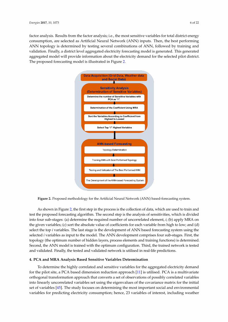
factor analysis. Results from the factor analysis; i.e., the most sensitive variables for total district energyconsumption, are selected as Artificial Neural Network (ANN) inputs. Then, the best performingANN topology is determined by testing several combinations of ANN, followed by training andvalidation. Finally, a district level aggregated electricity forecasting model is generated. This generatedaggregated model will provide information about the electricity demand for the selected pilot district.The proposed forecasting model is illustrated in Figure 2.

Figure 2. Proposed methodology for the Artificial Neural Network (ANN) based-forecasting system.

As shown in Figure 2, the first step in the process is the collection of data, which are used to train andtest the proposed forecasting algorithm. The second step is the analysis of sensitivities, which is dividedinto four sub-stages: (a) determine the required number of uncorrelated element, i; (b) apply MRA onthe given variables; (c) sort the absolute value of coefficients for each variable from high to low; and (d)select the top i variables. The last stage is the development of ANN based forecasting system using theselected i variables as input to the model. The ANN development comprises four sub-stages. First, thetopology (the optimum number of hidden layers, process elements and training functions) is determined.Second, the ANN model is trained with the optimum configuration. Third, the trained network is testedand validated. Finally, the tested and validated network is utilised in real-life predictions.

4. PCA and MRA Analysis Based Sensitive Variables Determination

To determine the highly correlated and sensitive variables for the aggregated electricity demandfor the pilot site, a PCA based dimension reduction approach [11] is utilised. PCA is a multivariateorthogonal transformation approach that converts a set of observations of possibly correlated variablesinto linearly uncorrelated variables set using the eigenvalues of the covariance matrix for the initialset of variables [45]. The study focuses on determining the most important social and environmentalvariables for predicting electricity consumption; hence, 23 variables of interest, including weather

Energies 2017, 10, 1073 7 of 22

conditions and social variables are selected for PCA. Eight out 23 variables, as shown in Figure 3,have been found as uncorrelated, indicating that these variables impact on the outputs independentlywithout sharing information among each other; i.e., they are uncorrelated.

Figure 3. Determination of the number of uncorrelated components with Principal Component Analysis(PCA).

The next step is to determine the coefficients of the selected eight variables using a multi regressionanalysis (MRA) as in Equation (1).

f (x) = Ax (1)

where A is coefficient vector AT = [a1 a2 . . . an ], x is variable vector XT = [x1 x2 . . . xn] and f (x) is thetotal grid energy consumption for next 30 min.

According to the MRA, the eight highest coefficient values are found for variables: currentelectricity consumption, outdoor air temperature, outdoor humidity, wind speed, outdoor air pressure,visibility, wind direction and number of the occupant under the age of fifteen.

5. Determination of the Best-Performed ANN Topology

As highlighted in Section 3, the main objective of the topology determination process is to find thebest performing ANN architecture for each individual ANN model which contributes in parallel to theaggregated district energy consumption. Each proposed ANN model has eight sensitive variables andfour-time information as ANN inputs and one output for the next thirty minutes’ energy consumption.In the proposed forecasting system, six parallel ANN models have been proposed to predict theaggregated energy demand. The cumulative forecasted energy demand provides the expected districtenergy consumption for this building cluster. The proposed ANN architecture with inputs and outputsis given in Figure 4.

Figure 4. Proposed ANN architecture for each building.

Energies 2017, 10, 1073 8 of 22

According to Figure 4, each proposed ANN model has twelve inputs which are: month, day,hour, minute, outdoor air temperature, outdoor humidity, outdoor air pressure, wind speed, winddirection, visibility, number of occupants under the age of fifteen (e.g., zero, one, two, three, and soon), and current energy consumption; and single output as next thirty minutes’ energy consumption.In the proposed parallel ANN model, Buildings 1, 4 and 6 have 0 occupants under age of 15; Building2 has three occupants who are under age of 15, who are also under age of 5 (they are staying in thehouse more than 6 h during the day); Building 3 has two occupants under age of 15, who are alsoabove the age of 5 (they are not staying in the house more than 6 h during the day); and Building 5has one occupant under age of 15, who is also under age of 5 (he/she is staying in the house morethan 6 h during the day). Although PCA-MRA based pre-processing did not correlate electricityconsumption and the opinion about the buildings’ temperature (i.e., if they were adequately warmedup), the authors wanted to see if there was a relationship among them by investigating the householdbudget, a proxy indicator for fuel poverty. As per rich data (i.e., questionnaire survey), respondentsfrom all households believed that their houses were adequately warmed up and the ratio of annualfuel expenses and annual household income was less than 0.1 or 10%, the fuel poverty threshold.The historical energy consumption data were for 18 months. The first year’s data were used for training,while the remaining six months’ electricity consumption data were utilised for testing and validation.

The training process for each building started with the determination of the best-performedtraining algorithm, as illustrated in in Table 1, while keeping the other variables constant;e.g., maximum number of iteration as 5000; the learning rate as 0.01; and the momentum coefficient as0.95. In addition, the number of hidden layers is kept as two, the numbers of the process elements ineach hidden layer are kept as 25 for both layers, and the transfer function types in both two hiddenlayers and the output layer are selected as logarithmic sigmoid with maximum epoch number of 5000with 10 repetitive runs. Further, the mean square error (MSE) for the parameter tuning during thetraining stage is set to 0.001, to keep the training error as low as possible. In this case, this value isfound as 0.001 with empirical tests. Moreover, the dataset is normalised between 0 and 1.

Table 1. Training algorithms used for the experiments.

No Abbreviation Definition

1 trainbfg Broyden, Fletcher, Goldfarb, and Shanno (BFGS) quasi-Newton backpropagation [46].2 traincgb Conjugate gradient backpropagation with Powell-Beale restarts [47].3 traincgf Conjugate gradient backpropagation with Fletcher-Reeves updates [47].4 traincgp Conjugate gradient backpropagation with Polak–Ribiere updates5 traingd Gradient descent backpropagation [46].6 traingda Gradient descent with adaptive learning rate backpropagation [46].7 traingdm Gradient descent with momentum backpropagation [46].8 traingdx Gradient descent with momentum and adaptive learning rate [46].9 trainlm Levenberg–Marquardt backpropagation [47].

10 trainscg Scaled conjugate gradient algorithm based on conjugate directions [46]

The average results of 10 runs for each ANN model are given in Table 2. The best performedANN was found for all six buildings with trainlm based algorithm (No. 9 in Table 1) [47]. Hereafter,further experiments will be carried with this algorithm (determined value) using other parameters(number of hidden layers, number of process elements in hidden layers and transfer function) wherethe initialised values of other parameters will be updated one by one in further stages.

The next stage is to find the required number of the hidden layers for the best performed ANN.To determine the optimum number of hidden layers, one, two, and three hidden layers are tested foreach building with ten repetitive runs. The average results of ten runs for each building are presentedin Table 3.

According to the testing results presented in Table 4, the best-performed topology has been foundwith the combination of [Logsig-Logsig-Logsig] in both hidden layers and output layers. In some

Energies 2017, 10, 1073 9 of 22

cases, some other combinations also provided desired target level but none of them performed betterthan the [Logsig-Logsig-Logsig] combination. This combination satisfied the desired target level for allsix ANN models with lowest epoch numbers. In the following experiments, this combination will beutilised alongside previous best-performed parameters. The last step of the topology determinationprocess is to find the best-performed number of process elements in the hidden layers. To perform thisexperiment, several combinations of the process elements are utilised in hidden layers for each ANNmodel. These combinations and the average results for the repetitive runs are given in Table 5.

Table 2. Training algorithm performance for each individual ANN model.

NoTraining

AlgorithmExpected

MSEANN Performance (Error/Epoch)

ANN1 ANN2 ANN3 ANN4 ANN5 ANN6

1 trainbfg 0.0010.004 0.201 0.121 0.094 0.329 0.0885000 5000 5000 5000 5000 5000

2 traincgb 0.0010.006 0.219 0.184 0.051 0.091 0.0475000 5000 5000 5000 5000 5000

3 traincgf 0.0010.004 0.192 0.106 0.037 0.101 0.0145000 5000 5000 5000 5000 5000

4 traincgp 0.0010.003 0.103 0.011 0.003 0.002 0.0085000 5000 5000 5000 5000 5000

5 traingd 0.0010.031 0.171 0.149 0.094 0.114 0.0625000 5000 5000 5000 5000 5000

6 traingda 0.0010.982 0.144 0.098 0.091 0.117 0.0425000 5000 5000 5000 5000 5000

7 traingdm 0.0010.727 0.083 0.020 0.026 0.112 0.0135000 5000 5000 5000 5000 5000

8 traingdx 0.0010.509 0.016 0.011 0.041 0.082 0.0095000 5000 5000 5000 5000 5000

9 trainlm 0.0010.001 0.001 0.001 0.001 0.001 0.001200 4836 1601 985 460 309

10 trainscg 0.0010.003 0.167 0.004 0.005 0.002 0.0045000 5000 5000 5000 5000 5000

Table 3. Experiments for the number of hidden layer.

Number ofHidden Layer

ExpectedMSE

ANN Performance (Error/Epoch)

ANN1 ANN2 ANN3 ANN4 ANN5 ANN6

1 0.0010.001 0.002 0.002 0.001 0.001 0.0011002 5000 5000 3712 1941 2907

2 0.0010.001 0.001 0.001 0.001 0.001 0.001278 413 372 291 276 294

3 0.0010.001 0.003 0.002 0.002 0.002 0.0023073 5000 5000 5000 5000 5000

According to Table 3, some experiments achieved the targets with one and three hidden layers forsome buildings (coloured in grey), but the best performed ANNs were found with two hidden layersfor each building specific ANNs, with the lowest number of iterations. Moreover, ANN for Building1 achieved the target MSE (0.001) with 278 epochs. Similarly, energy consumption for Buildings 2–6has been found after 413, 372, 291, 276 and 294 epochs, respectively. Based on the experiments, thetopology optimisation will be carried out using two hidden layers.

The next stage of the experiments is the determination of the transfer function in both hidden andoutput layers. Three types of transfer functions are being considered—hyperbolic tangent sigmoidfunction (tansig), logarithmic sigmoid function (logsig) to include nonlinearity in the learning process,and linear transfer function (purelin) to transform a linear mapping between inputs and outputs.

Energies 2017, 10, 1073 10 of 22

The experiments were conducted with ten repetitive runs for each selected configuration, and theaverage results are shown in Table 4.

Table 4. Experiments for the transfer functions in hidden layers and output layer.

Transfer Functions inHidden and Output Layers

ExpectedMSE

ANN Performance (Error/Epoch)

ANN1 ANN2 ANN3 ANN4 ANN5 ANN6

(Tansig-Tangsig-Tansig) 0.00100.0378 0.0922 0.0474 0.0497 0.0398 0.03515000 5000 5000 5000 5000 5000

(Tansig-Tansig-Logsig) 0.00100.0009 0.0026 0.0012 0.0010 0.0032 0.0021

812 5000 5000 3864 5000 5000

(Tansig-Tansig-Purelin) 0.00100.1604 0.2441 0.1712 0.2099 0.1796 0.21045000 5000 5000 5000 5000 5000

(Tansig-Logsig-Tansig) 0.00100.0009 0.0010 0.0010 0.0009 0.0010 0.0010

377 511 701 292 643 665

(Tansig-Logsig-Logsig) 0.00100.0009 0.0010 0.0010 0.0010 0.0010 0.0009

278 339 517 415 1009 423

(Tansig-Logsig-Purelin) 0.00100.1039 0.1832 0.1591 0.1903 0.1505 0.09395000 5000 5000 5000 5000 5000

(Tansig-Purelin-Tansig) 0.00100.0159 0.0479 0.0270 0.0188 0.0252 0.01635000 5000 5000 5000 5000 5000

(Tansig-Purelin-Logsig) 0.00100.0174 0.1097 0.0053 0.0221 0.0036 0.00565000 5000 5000 5000 5000 5000

(Tansig-Purelin-Purelin) 0.00100.3571 0.3239 0.2962 0.3027 0.3308 0.29915000 5000 5000 5000 5000 5000

(Logsig-Tangsig-Tansig) 0.00100.0012 0.0027 0.0010 0.0010 0.0019 0.00115000 5000 4517 4882 5000 5000

(Logsig-Tansig-Logsig) 0.00100.0009 0.0010 0.0010 0.0009 0.0010 0.001

202 1022 633 711 490 318

(Logsig-Tansig-Purelin) 0.00100.3290 0.3782 0.3592 0.3882 0.3113 0.29775000 5000 5000 5000 5000 5000

(Logsig-Logsig-Tansig) 0.00100.0010 0.0011 0.0009 0.0010 0.0009 0.0015

298 5000 578 3049 2610 5000

(Logsig-Logsig-Logsig) 0.00100.001 0.001 0.001 0.001 0.001 0.001181 247 214 197 243 252

(Logsig-Logsig-Purelin) 0.00100.2427 0.2917 0.2541 0.2351 0.3132 0.26695000 5000 5000 5000 5000 5000

(Logsig-Purelin-Tansig) 0.00100.1041 0.2044 0.1185 0.1670 0.1112 0.10705000 5000 5000 5000 5000 5000

(Logsig-Purelin-Logsig) 0.00100.0928 0.2029 0.1081 0.0956 0.0996 0.11265000 5000 5000 5000 5000 5000

(Logsig-Purelin-Purelin) 0.00100.2039 0.3017 0.3431 0.2982 0.3272 0.27785000 5000 5000 5000 5000 5000

(Purelin-Tangsig-Tansig) 0.00100.1652 0.2931 0.1982 0.1771 0.2028 0.17145000 5000 5000 5000 5000 5000

(Purelin-Tansig-Logsig) 0.00100.1038 0.1213 0.0942 0.1675 0.1119 0.10035000 5000 5000 5000 5000 5000

(Purelin-Tansig-Purelin) 0.00100.2611 0.3498 0.4192 0.3111 0.2991 0.35855000 5000 5000 5000 5000 5000

(Purelin-Logsig-Tansig) 0.00100.1779 0.0962 0.1137 0.1042 0.2783 0.10175000 5000 5000 5000 5000 5000

(Purelin-Logsig-Logsig) 0.00100.1399 0.1049 0.3288 0.1414 0.0973 0.14405000 5000 5000 5000 5000 5000

(Purelin-Logsig-Purelin) 0.00100.2862 0.4492 0.2961 0.3038 0.2977 0.39325000 5000 5000 5000 5000 5000

(Purelin-Purelin-Tansig) 0.00100.1291 0.3912 0.1193 0.3216 0.1973 0.10425000 5000 5000 5000 5000 5000

(Purelin-Purelin-Logsig) 0.00100.2357 0.2190 0.4971 0.2933 0.4349 0.33535000 5000 5000 5000 5000 5000

(Purelin-Purelin-Purelin) 0.00100.3422 0.4731 0.4491 0.3702 0.4944 0.37305000 5000 5000 5000 5000 5000

Energies 2017, 10, 1073 11 of 22

Table 5. Experiments for the number of process elements in hidden layers.

Number ofHidden Layer

ExpectedMSE

ANN Performance (Error/Epoch)

ANN1 ANN2 ANN3 ANN4 ANN5 ANN6

(5 5) 0.0010.0010 0.0024 0.0027 0.0010 0.001 0.0011002 5000 5000 3712 1941 2907

(5 15) 0.0010.0010 0.001 0.0010 0.001 0.001 0.001

348 213 72 191 276 494

(5 25) 0.0010.0010 0.0034 0.0029 0.0020 0.0021 0.00243073 5000 5000 5000 5000 5000

(5 30) 0.0010.0011 0.0029 0.0023 0.0010 0.0010 0.00105000 5000 5000 3712 1941 2907

(15 5) 0.0010.0011 0.0014 0.0011 0.0010 0.0011 0.00105000 5000 5000 4817 5000 4011

(15 15) 0.0010.0010 0.0009 0.0009 0.001 0.001 0.002

278 112 96 114 203 161

(15 25) 0.0010.0090 0.0010 0.0009 0.0010 0.001 0.001

172 19 4 82 119 107

(15 30) 0.0010.001 0.0010 0.0010 0.0010 0.0010 0.0010412 113 179 162 76 19

(25 5) 0.0010.001 0.0021 0.0015 0.0012 0.0011 0.00103073 5000 5000 5000 5000 3218

(25 15) 0.0010.0010 0.0010 0.0010 0.0010 0.0010 0.0010

198 112 101 87 134 68

(25 25) 0.0010.0010 0.0010 0.0010 0.0010 0.0010 0.0010

221 49 31 109 92 54

(25 30) 0.0010.0010 0.0010 0.0010 0.0010 0.0010 0.0010

174 43 64 101 98 66

(30 5) 0.0010.0010 0.0012 0.0010 0.0011 0.0010 0.0010

714 5000 3810 5000 2423 968

(30 15) 0.0010.0010 0.0010 0.0010 0.0010 0.0010 0.0010

403 1541 56 1009 118 86

(30 25) 0.0010.0010 0.0010 0.0010 0.0010 0.0010 0.0010

198 91 39 88 300 129

(30 30) 0.0010.0010 0.0010 0.0010 0.0010 0.0010 0.0010

203 42 101 96 1941 114

According to Table 5, the desired MSE was found in most cases; the best-performed ones arecoloured in blue and presented in bold font. The others that achieved the desired MSE level arecoloured grey. The best-performed ones are the ones that met the desired MSE with the lowest numberof the epochs. The selected topology for each ANN model is presented in Table 6.

Table 6. Final topology for each ANN model.

ANN No The TrainingFunction

The NumberHidden Layer

Transfer Function Type inHidden and Output Layers

The Number of ProcessElement in Hidden Layer

ANN for Building1 trainlm 2 (Logsig-Logsig-Logsig) (15 25)ANN for Building2 trainlm 2 (Logsig-Logsig-Logsig) (15 25)ANN for Building3 trainlm 2 (Logsig-Logsig-Logsig) (15 25)ANN for Building4 trainlm 2 (Logsig-Logsig-Logsig) (15 25)ANN for Building5 trainlm 2 (Logsig-Logsig-Logsig) (15 30)ANN for Building6 trainlm 2 (Logsig-Logsig-Logsig) (15 30)

Since the ANN development is a data driven process, configurations presented in Tables 2–6are dependent on the datasets. Configurations and MSEs are, therefore, not guaranteed fordifferent datasets. Moreover, this configuration cannot be generalised in some parameter. However,

Energies 2017, 10, 1073 12 of 22

Yuce et al. [23] stated that trainlm based training function performs the best in electricity managementproblems; and that other configurations do not seem to have similar performance.

6. Results and Discussion

The proposed ANN models are developed and tested in a computer with Intel TM Core i5 2.27GHz processor and 4 GB memory. MATLAB 2016a was used as the software platform. As per Table 6,the best-performed training algorithm is Levenberg-Marquart for every ANN model with two hiddenlayers. The logarithmic sigmoid transfer function is used in both hidden and output layers. Finally, thenumber of the process elements for each hidden layer are (15 20), (15 20), (15 20), (15 20), (15 30), and(15 30) for the ANN of Buildings 1–6, respectively. Training performance of these best performed ANNmodels is illustrated in Figures 5–10 by comparing with expected electricity consumption (expectedelectricity consumption is the actual electricity consumption which is occurred after 30 min from thecorresponding prediction time frame) for a typical day of each season.

Figure 5. Comparison between the actual and predicted electricity consumption for the training resultsof ANN1 for a typical day in four seasons: (a) winter; (b) spring; (c) summer; and (d) autumn.

Figure 6. Comparison between the actual and predicted electricity consumption for the training resultsof ANN2 for a typical day in four seasons: (a) winter; (b) spring; (c) summer; and (d) autumn.

Energies 2017, 10, 1073 13 of 22

Figure 7. Comparison between the actual and predicted electricity consumption for the training resultsof ANN3 for a typical day in four seasons: (a) winter; (b) spring; (c) summer; and (d) autumn.

Figure 8. Comparison between the actual and predicted electricity consumption for the training resultsof ANN4 for a typical day in four seasons: (a) winter; (b) spring; (c) summer; and (d) autumn.

Results presented in Figures 5–10 demonstrate the accuracy of the developed ANN for a typicalday, which is the middle day of each season, for each building. The error rate for this selected day isfound based on the average percentage error, computed based on the Equation (2).

Average Percentage Error = 100 ∗ |Expected Electricity Consumption −Predicted Electricity Consumption|Expected Electricity Consumption (2)

Further, an error analysis is carried out to determine the accuracy of the training processfor each ANN using the average percentage error for the selected period (one year); the resultsare presented in Table 7. Moreover, the correlation between the predicted demand and expectedelectricity consumption (it is the actual electricity consumption which is occurred after 30 min from thecorresponding prediction time frame) are statistically analysed using Pearson correlation coefficientand regression analysis.

Energies 2017, 10, 1073 14 of 22

Figure 9. Comparison between the actual and predicted electricity consumption for the training resultsof ANN5 for a typical day in four seasons: (a) winter; (b) spring; (c) summer; and (d) autumn.

Figure 10. Comparison between the actual and predicted electricity consumption for the trainingresults of ANN6 for a typical day in four seasons: (a) winter; (b) spring; (c) summer; and (d) autumn.

Table 7. Training error analysis of each proposed ANN models.

ANN AveragePercentage Error

Pearson CorrelationCoefficient R2 Constant

Coefficient (a)Variable

Coefficient (b)

ANN1 4.03 0.999 0.997 1.85 × 10−5 0.998ANN2 15.81 0.973 0.946 0.000 0.907ANN3 9.03 0.998 0.996 −2.44 × 10−5 1.090ANN4 5.51 0.999 0.998 0.001 1.053ANN5 7.05 0.999 0.997 0.000 1.070ANN6 4.07 0.998 0.997 0.001 0.990

According to Table 7, all Pearson correlation coefficients are found greater than 0.90 for thepredicted and the expected results, demonstrating a high correlation between the predicted andexpected values. Further, the best performing ANN results are found with Building 1 with 4.03%average percentage error. The high accuracy of ANN for the Building 1 can also be seen based on the

Energies 2017, 10, 1073 15 of 22

linear regressions coefficient as shown in Table 7. In this paper, the linear regression model for thisproblem is presented as in Equation (3).

Expected Energy Consumption = a + b(Predicted Energy Consumption) (3)

Based on Equation (3), the expected energy consumption for Building 1 almost equals to thepredicted energy consumption by including “a” as 1.85 × 10−5 and “b” as 0.998. Moreover, coefficientsfor Building 2 are also verified that the performance of ANN for Building 2 is the least accurateone, which has three children under the age of fifteen who are also under the age of five. Moreover,according to the comparison between buildings based on the number of children occupant, Building 2consists of three children under the age of five (who are staying at home more than 6 h during the day)with the average percentage error of 15.81%, which is 6.78% higher than the average percentage errorfound in Building 3 that consists of two children who are under age of fifteen and not staying at homemore than 6 h during the day (age > 5 years). According to the comparison between Buildings 3 and5 (one child, who does not stay at home more than 6 h during the day), the error difference is foundas 1.98%. Based on this result, the difference between the error of Buildings 2 and 3 is about threetimes greater than the error of the difference between Buildings 3 and 5. It was challenging to achieveprediction results for the buildings with irregular energy consumption patterns. This expectationis confirmed with both average percentage error and linear regression analysis. The building withno children under age fifteen has a regular energy consumption pattern compared to the buildingswith children under age of fifteen. However, the prediction error is lower in the aggregated energyconsumption. The aggregated energy consumption prediction error for these six buildings is foundas 4.33%. This result shows that the error level in the building level can vary under different scales.However, this variation is much lower in the aggregated electricity compared to the building level.Prediction in some time stamp can be higher for one building while potentially lower in another. Hence,the effect of the prediction variation stays lower during the aggregation, as illustrated in Figure 11.

In Figure 11, the red and blue coloured lines denote the expected total (i.e., aggregated)energy consumption and the total predicted energy consumption for six buildings, respectively.The aggregation is accomplished by adding together all buildings’ electricity consumption. The trainingstage’s aggregated forecast accurately traces the aggregated expected electricity consumption.

Further analysis is carried out for the testing stage of the developed ANN models for eachbuilding. The average percentage error, Pearson correlation coefficient and regression analysis basedcomparison are illustrated in Table 8.

Figure 11. Comparison between the results of the aggregated actual and the aggregated predictedelectricity demand for the training stage.

Energies 2017, 10, 1073 16 of 22

Table 8. Testing error analysis of each ANNs.

ANN No AveragePercentage Error

Pearson CorrelationCoefficient R2 Value

ConstantCoefficient

VariableCoefficient

ANN1 6.51 0.999 0.998 0.000 1.065ANN2 22.64 0.992 0.984 −0.001 1.227ANN3 14.45 0.996 0.992 0.002 1.135ANN4 9.95 0.997 0.994 0.002 1.095ANN5 14.17 0.995 0.990 0.001 1.138ANN6 12.07 0.997 0.994 −0.002 1.124

As illustrated Table 8, the testing results for Building 1 is found best compared to other buildingresults. As Building 1 does not have any children under age of 15, the better prediction is obtainedcompared to other buildings. Hence, the results are expected to be lowest. However, this result isexpected for Buildings 4 and 6 too. However, their prediction results slightly worse compare to theBuilding 1. In addition, they have also better accuracy rate compare to buildings than the Buildings3 and 5. This result is also verify based on the linear regression coefficients. The results for theBuilding 2 are still found the worst results in Table 8 (red font). This is also expected since thisbuilding consists of occupants which are 3 children under age of 15 and adults. According to the linearregression coefficients, the best prediction results during the testing stage are found with the Building1. This result shows that an expected result is equal to 1.065 times of the predicted result. Finally, theaggregated results for the testing stage are also illustrated in Figure 12.

According to the error analysis between the aggregated expected electricity and the aggregatedpredicted results, it has been found that the average percentage error is 13.41% which is the average ofthe errors presented in Column 2 of Table 8. Although this result is slightly higher than the averageerrors of the Building 1 and 6, the results are still lower than the rest of the buildings’ results. Thisoutput also verifies that the aggregated prediction results are still less affected compared to individualbuildings (apart from Buildings 1 and 6). The worst average percentage was found for Building 2 as22.64%, computed based on the average percentage differences between expected and predicted values.A detailed analysis of existing literature and proposed study is presented in Table 9 to demonstrate themain contribution.

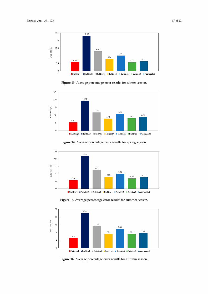
Finally, an analysis is carried out on the average error for each building in different seasons.The entire period’s (1.5 year, including training and testing time periods) predicted and expectedconsumption are considered in this analysis. The results are illustrated for winter, spring, summerand autumn seasons in Figures 13–16, respectively. Spring season has the highest average percentageerror, compared to other seasons, for every building and the aggregation, while the results for autumnseason have the lowest average percentage error for every building and the aggregation. The electricityconsumption during winter season appears to have a consistent profile. On the other hand, theconsumption profiles are intermittent during spring, regardless of the occupancy type.

Figure 12. Comparison between the results of the aggregated actual and the aggregated predictedelectricity demand for the testing stage.

Energies 2017, 10, 1073 17 of 22

Figure 13. Average percentage error results for winter season.

Figure 14. Average percentage error results for spring season.

Figure 15. Average percentage error results for summer season.

Figure 16. Average percentage error results for autumn season.

Energies 2017, 10, 1073 18 of 22

Table 9. ANN parameter comparison between the proposed work and existing literature.

Proposed Study ANN TypeInput

SelectionMethod

WeatherInput

TimeInput

SocialVariables

ParameterTuning

BuildingLevel

GridLevel

SeasonalAnalysis

Proposed Study MLP SensitivityAnalysis Yes Yes Yes Yes Yes Yes Yes

Yuce et al. [11] MLP SensitivityAnalysis Yes Yes No Yes Yes No No

Mocanu et al. [21] MLP Empirical No No No Yes Yes No No

Yuce et al. [23] MLP SensitivityAnalysis Yes Yes No Yes Yes No No

Hernandez et al. [26] MLP Empirical No No No No No Yes No

Srinivasan, [27] MLP Empirical Yes No No No No Yes No

Kalaitzakis et al. [28] MLP, RBF, ARNNand RAWN Empirical No No No No No Yes No

Rodrigues et al. [29] MLP Empirical No No No No Yes No No

Chen et al. [30] MLP Empirical No No No No No Yes No

As shown in Table 9, the proposed study has demonstrated a systematic approach for ANNdevelopment and implementation for the smart grid domain both using a sensitivity analysis for theinput parameter selection, social variables involvement and analysis in seasonal levels (coloured as bluein the above table). Further, the proposed study also presents the usage of the parallel ANN processin the grid level which is assumed as single ANN model in the other literature studies. The detailedconclusion is presented in Section 7.

7. Conclusions and Limitations

The main objective of this study is to develop an accurate and robust ANN-based forecastingmodels (in parallel performing ANNs) for the sub-hourly prediction of the electricity consumptionin district-level which consists of multiple building based consumers; moreover, this informationis then aimed to utilise in the smart grid domain. Further, the average accuracy of forecastingsystem will also be used to adjust the demand’s flexibility at Aggregator and DSO levels; hence, thehigh accuracy of the forecasting systems is the key approach. To achieve high accuracy with theforecasting, the objective of the study was enhanced with the accuracy analysis in different seasons,and varying occupant types. Moreover, the study was also aimed to demonstrate a systematicapproach to the development parallel ANNs including a sensitivity approach to determine theinputs of ANN and implementing an experimental design to optimise the topology among multipleconfiguration types. Using a systematic approach during the ANN development stage and stating theaccuracy differences in different seasons will provide the aggregator and DSO operators to updatetheir demand flexibility and adjust their loads during the pick hours based the provided limits. Further,results for buildings with different occupancy types provide the Aggregator and DSO operators tohave adaptive demand flexibilities. Hence, the proposed model is implemented on six buildings,with different characteristics and occupancy type. The development of the ANN-based electricitydemand forecasting model started with the topology determination; i.e., the identification of themost appropriate ANN inputs. Sensitivities of electricity consumption and environmental variablesare conducted using Principal Component Analysis (PCA) and Multi-Regression Analysis (MRA).The remaining topology parameters such as the number of hidden layers, number of processes inhidden layers, transfer function types and the training algorithm are found through several parametricexperiments. The topology analysis is carried out for each individual ANN model, followed by modeltraining and testing. The model is developed and tested on the Irish Smart Grid dataset comprisingmonitored electricity consumption data for 18 months.

Results indicate that the prediction of electricity consumption of residential buildings withchildren aged up to fifteen is harder than the buildings occupied only by adults. However,the aggregated electricity demand prediction has a lower prediction average percentage error

Energies 2017, 10, 1073 19 of 22

(i.e., less sensitive) compared to the individual buildings. With regards to seasonal predictions, theaverage percentage error is lower during winter, while autumn season has the highest averagepercentage error. Irregular demand for electricity during autumn may be attributed as the reason.Since peak demand prediction is critical for the district-level electricity management, greater accuracyof prediction is important if the district is to incorporate flexibility in management. The accuracy ofthe prediction is, therefore, investigated in detail, including the effects of occupancy type and season.The worst average prediction average percentage error is found as 19.18% during spring for buildingsoccupied by children under age of 15. The lowest average percentage error is found as 4.06% with thebuilding with no children under age of 15 for winter. Further, the lowest average percentage error forthe aggregated electricity consumption is found for winter (4.51%) and the highest average percentageerror (8.82%) is found for spring. The accuracy of the proposed model is highly depending on theconsistency of the data: if the existing data are not very representative, than the accuracy will be lowerthan the accuracy of a well-correlated dataset. Since the ANN-based forecasting system is also problemspecific, the scenario changes, which means changes in the dataset, will affect the ANN topology andconfiguration even if the inputs and outputs will remain the same. Hence, the generalisation of thedata with ANN is not possible unless the training process with the new problem is conducted with theproposed methodology.

Research reported in this paper is one of the very few on the importance of social and/ordemographical characteristics on forecasting electricity consumption in the distribution grid. With theincreased penetration of variable renewable energy resources, having an accurate forecasting ofdemand at the substation level and below becomes important. The effectiveness of social variables inpredicting average and peak demand is successfully highlighted here; however, the main limitationis related to the lack of detailed information about fuel poverty. Although the householders’ generalopinion was that the indoor temperature was adequate, it was not clear how and whether fuelpoverty affected their consumption signature. Details on energy expenses, household budgets,and home level appliances can provide a better estimation, which needs to be explored in futureresearch. The other challenge was related to the correlation of householders’ opinion with electricityconsumption. Quantitative estimates or measurements of indoor environmental conditions mayameliorate some of the related limitations. Furthermore, the measurement through the Irish Smart Gridtrial was carried out in 2012; hence, further information about the households’ energy consumptionand relevant social characteristics could not be gathered.

Finally, it is found that ANN-based forecasting solution is performing very well for the districtlevel energy prediction. This approach is very sensitive with irregular patterns; hence, the selection ofdata or pre-processing of the data is the key to reducing estimation errors. However, this approachmay still not be enough to achieve a better solution with ANN on irregular datasets. It may be requiredto utilise statistical or other data mining solution to tackle these types of datasets such as predictiveclassification algorithms or high-order time series techniques.

Acknowledgments: The authors acknowledge the financial support of the European Commission in the contextof the MAS2TERING project (Grant ref.: 619682), funded under the ICT-2013.6.1—Smart Energy Grids program.

Author Contributions: Baris Yuce and Monjur Mourshed conceived and designed the experiments; Baris Yuceperformed the experiments; Baris Yuce and Monjur Mourshed analysed the data and interpreted the results; andall authors contributed to the writing up of the paper.

Conflicts of Interest: The authors declare no conflict of interest. The funding sponsors had no role in the designof the study; in the collection, analyses, or interpretation of data; in the writing of the manuscript, and in thedecision to publish the results.

Energies 2017, 10, 1073 20 of 22

References

1. Pearson, P.J.G.; Foxon, T.J. A low carbon industrial revolution? Insights and challenges from pasttechnological and economic transformations. Energy Policy 2012, 50, 117–127. [CrossRef]

2. EUREL. Electrical Power Vision 2040 for Europe; EUREL General Secretariat: Brussels, Belgium, 2012; Availableonline: http://www.eurel.org/home/TaskForces/Pages/PowerVision2040(completed).aspx (accessed on10 September 2016).

3. European Communities (EC). European Technology Platform Smart Grids: Vision and Strategy for Europe’sElectricity Networks of the Future; Office for Official Publications of the European Communities: Brussels,Belgium, 2016; Available online: https://ec.europa.eu/research/energy/pdf/smartgrids_en.pdf (accessedon 10 September 2016).

4. European Communities (EC). SET Plan- Towards an Integrated Roadmap: Research & Innovation Challengesand Needs of the EU Energy System; European Communities: Brussels, Belgium, 2014; Available online:https://setis.ec.europa.eu/system/files/Towards%20an%20Integrated%20Roadmap_0.pdf (accessed on10 September 2016).

5. Farhangi, H. The path of the smart grid. IEEE Mag. Power Energy 2010, 8, 18–28. [CrossRef]6. Mourshed, M.; Robert, S.; Ranalli, A.; Messervey, T.; Reforgiato, D.; Contreau, R.; Becue, A.; Quinn, K.;

Rezgui, Y.; Lennard, Z. Smart Grid Futures: Perspectives on the Integration of Energy and ICT Services.Energy Procedia 2015, 75, 1132–1137. [CrossRef]

7. Brusco, G.; Burgio, A.; Menniti, D.; Pinnarelli, A.; Sorrentino, N. Energy Management System for an EnergyDistrict with Demand Response Availability. IEEE Trans. Smart Grid 2014, 5, 2385–2393. [CrossRef]

8. Chao, H.L.; Tsai, C.C.; Hsiung, P.A.; Chou, I.H. Smart Grid as a Service: A Discussion on Design Issues.Sci. World J. 2014, 2014, 1–11. [CrossRef] [PubMed]

9. European Communities (EC). An Introduction to the Universal Smart Energy Framework (USEF); Smart EnergyCollective: Arnhem, The Netherlands, 2013; Available online: https://ec.europa.eu/energy/sites/ener/files/documents/xpert_group3_summary.pdf (accessed on 10 September 2016).

10. Patti, E.; Ronzino, A.; Osello, A.; Verda, V.; Acquaviva, A.; Macii, E. District Information Modeling andEnergy Management. IT Prof. 2015, 17, 28–34. [CrossRef]

11. Yuce, B.; Rezgui, Y.; Mourshed, M. ANN-GA smart appliance scheduling for optimized energy managementin the domestic sector. Energy Build. 2016, 111, 311–325. [CrossRef]

12. Fonseca, J.A.; Nguyen, T.A.; Schlueter, A.; Marechal, F. City Energy Analyst (CEA): Integrated frameworkfor analysis and optimization of building energy systems in neighborhoods and city districts. Energy Build.2016, 113, 202–226. [CrossRef]

13. Fanti, M.P.; Mangini, A.M.; Roccotelli, M.; Ukovich, W.; Pizzuti, S. A control strategy for district energymanagement. In Proceedings of the IEEE International Conference on Automation Science and Engineering(CASE), Gothenburg, Sweden, 24–28 August 2015; pp. 432–437.

14. Van Pruissen, O.; Van der Togt, A.; Werkman, E. Energy Efficiency Comparison of a Centralized anda Multi-Agent Market Based Heating System in a Field Test. Energy Procedia 2014, 62, 170–179. [CrossRef]

15. Powell, K.M.; Sriprasad, A.; Cole, W.J.; Edgar, T.F. Heating, cooling, and electrical load forecasting fora large-scale district energy system. Energy 2014, 74, 877–885. [CrossRef]

16. Van Hulle, F.; Fichaux, N.; Sinner, A.F.; Morthorst, P.E.; Munksgaard, J.; Ray, S. Powering Europe: Wind Energyand Electrical Grid; EWEA: Brussels, Belgium, 2010.

17. Jing, Z.X.; Jiang, X.S.; Wu, Q.H.; Tang, W.H.; Hua, B. Modelling and optimal operation of a small-scaleintegrated energy based district heating and cooling system. Energy 2014, 73, 399–415. [CrossRef]

18. Walker, R.; McKenzie, P.; Liddell, C.; Morris, C. Estimating fuel poverty at household level: An integratedapproach. Energy Build. 2014, 80, 469–479. [CrossRef]

19. Berangere, L.; Ricci, O. Measuring fuel poverty in France: Which households are the most fuel vulnerable?Energy Econ. 2015, 49, 620–628.

20. Yuce, B.; Li, H.; Rezgui, Y.; Petri, I.; Jayan, B.; Yang, C. Utilizing artificial neural network to predict energyconsumption and thermal comfort level: An indoor swimming pool case study. Energy Build. 2014, 80, 45–56.[CrossRef]

21. Mocanu, E.; Nguyen, P.H.; Gibescu, M.; Kling, W.L. Deep learning for estimating building energyconsumption. Sustain. Energy Grids Netw. 2016, 6, 91–99. [CrossRef]

Energies 2017, 10, 1073 21 of 22

22. Yang, C.; Li, H.; Rezgui, Y.; Petri, I.; Yuce, B.; Chen, B.; Jayan, B. High throughput computing baseddistributed genetic algorithm for building energy consumption optimization. Energy Build. 2014, 76, 92–101.[CrossRef]

23. Yuce, B.; Rezgui, Y. An ANN-GA semantic rule-based system to reduce the gap between predicted andactual energy consumption in buildings. IEEE Trans. Autom. Sci. Eng. 2015, 14, 1351–1363. [CrossRef]

24. Dibley, M.J.; Li, H.; Rezgui, Y.; Miles, J.C. An ontology framework for intelligent sensor-based buildingmonitoring. Autom. Constr. 2012, 28, 1–14. [CrossRef]

25. Kandananond, K. Forecasting Electricity Demand in Thailand with an Artificial Neural Network Approach.Energies 2011, 4, 1246–1257. [CrossRef]

26. Hernandez, L.; Baladron, C.; Aguiar, J.M.; Calavia, L.; Carro, B.; Sanchez-Esguevillas, A.; Perez, F.;Fernandez, A.; Lloret, J. Artificial Neural Network for Short-Term Load Forecasting in Distribution Systems.Energies 2014, 7, 1576–1598. [CrossRef]

27. Srinivasan, D. Evolving artificial neural networks for short term load forecasting. Neurocomputing 1998, 23,265–276. [CrossRef]

28. Kalaitzakis, K.; Stavrakakis, G.S.; Anagnostakis, E.M. Short-term load forecasting based on artificial neuralnetworks parallel implementation. Electr. Power Syst. Res. 2002, 63, 185–196. [CrossRef]

29. Rodrigues, F.; Cardeira, C.; Calado, J.M.F. The Daily and Hourly Energy Consumption and Load ForecastingUsing Artificial Neural Network Method: A Case Study Using a Set of 93 Households in Portugal.Energy Procedia 2014, 62, 220–229. [CrossRef]

30. Chen, C.S.; Tzeng, Y.M.; Hwang, J.C. The application of artificial neural networks to substation loadforecasting. Electr. Power Syst. Res. 1996, 38, 153–160. [CrossRef]

31. Lourenco, J.M.; Santos, P.J. Short Term Load Forecasting Using Gaussian Process Models; Institute of SystemEngineering and Computers (INESC): Coimbra, Portugal, 2010.

32. Hussain, L.; Nadeem, M.S.; Ali Shah, S.A. Short term load forecasting system based on support vector kernelmethods. Int. J. Comput. Sci. Inf. Technol. 2014, 6, 93–102. [CrossRef]

33. Barakati, S.M.; Gharaveisi, A.E.; Reza Rafiei, S.M. Short-term load forecasting using mixed lazy learningmethod. Turk. J. Electr. Eng. Comput. Sci. 2015, 23, 203–211. [CrossRef]

34. Dragomir, O.; Dragomir, F.; Gouriveau, R.; Minca, E. Medium term load forecasting using ANFIS predictor.In Proceedings of the 18th Mediterranean Conference on Control & Automation, MED’10, Marrakech,Morocco, 23–25 June 2010; pp. 551–556.

35. Badri, A.; Ameli, Z.; Birjandi, A.M. Application of Artificial Neural Networks and Fuzzy Logic Methods forShort Term Load Forecasting. Energy Procedia 2012, 14, 1883–1888. [CrossRef]

36. Ferreira, P.M.; Ruano, A.E.; Silva, S.M.; Conceicao, E.Z.E. Neural Networks Based Predictive Control forThermal Comfort and Energy Savings in Public Buildings. Energy Build. 2012, 55, 238–251. [CrossRef]

37. Xia, C.; Wang, J.; McMenemy, K. Short, medium and long-term load forecasting model and virtual loadforecaster based on radial basis function neural networks. Int. J. Electr. Power Energy Syst. 2010, 32, 743–750.[CrossRef]

38. Ahmad, M.W.; Mourshed, M.; Yuce, B.; Rezgui, Y. Computational intelligence techniques for HVAC systems:A review. Build. Simul. 2016, 9, 359–398. [CrossRef]

39. Grant, J.; Eltoukhy, M.; Asfour, S. Short-Term Electrical Peak Demand Forecasting in a Large GovernmentBuilding Using Artificial Neural Networks. Energies 2014, 7, 1935–1953. [CrossRef]

40. Valerio, A.; Giuseppe, M.; Gianluca, G.; Alessandro, Q.; Borean, C. Intelligent Systems for Energy ProsumerBuildings at District Level. In Proceedings of the 23rd International Conference on Electricity Distribution(CIRED), Lyon, France, 15–18 June 2015; pp. 1–5.

41. Idowu, S.; Saguna, S.; Ahlund, C.; Schelen, O. Forecasting heat load for smart district heating systems:A machine learning approach. In Proceedings of the 2014 IEEE International Conference on Smart GridCommunications (SmartGridComm), Venice, Italy, 2014; pp. 554–559.

42. Yue, H.; Dan, L.; Liqun, G. Power system short-term load forecasting based on neural network with artificialimmune algorithm. In Proceedings of the Control and Decision Conference (CCDC), Taiyuan, China,23–25 May 2012; pp. 844–848.

43. ISSDA. CER Smart Metering Project. Available online: http://www.ucd.ie/issda/data/commissionforenergyregulationcer/ (accessed on 10 September 2016).

Energies 2017, 10, 1073 22 of 22

44. Yuce, B.; Mourshed, M.; Rezgui, Y. An ANN-based energy forecasting framework for the district levelsmart grids. In Smart Grid Inspired Future Technologies; Hu, J., Leung, V.C.M., Yang, K., Zhang, Y., Gao, J.,Yang, S., Eds.; Springer: Berlin/Heidelberg, Germany, 2017; pp. 107–117.

45. Yuce, B.; Mastrocinque, E.; Packianather, M.S.; Pham, D.; Lambiase, A.; Fruggiero, F. Neural network designand feature selection using principal component analysis and Taguchi method for identifying wood veneerdefects. Prod. Manuf. Res. 2014, 2, 291–308.

46. Lahmiri, S. A Comparative Study of Backpropagation Algorithms in Financial Prediction. Int. J. Comput. Sci.Eng. Appl. 2011, 1, 15–21.

47. Shaharin, R.; Prodhan, U.Z.; Rahman, M. Performance Study of TDNN Training Algorithm for SpeechRecognition. Int. J. Adv. Res. Comput. Sci. Technol. 2014, 2, 90–95.

© 2017 by the authors. Licensee MDPI, Basel, Switzerland. This article is an open accessarticle distributed under the terms and conditions of the Creative Commons Attribution(CC BY) license (http://creativecommons.org/licenses/by/4.0/).