a small-order-polynomial-sized linear program for solving ... · a small-order-polynomial-sized...
TRANSCRIPT

Exact extended formulation of the linear assignmentproblem (LAP) polytope for solving the travelingsalesman and quadratic assignment problems
Moustapha DiabyOPIM Department; University of Connecticut; Storrs, CT 06268
Mark H. KarwanDepartment of Industrial and Systems Engineering; SUNY at Buffalo; Amherst, NY 14260
Lei SunDepartment of Industrial and Systems Engineering; SUNY at Buffalo; Amherst, NY 14260
Abstract: We present an O(n6 ) linear programming model for the traveling salesman (TSP)and quadratic assignment (QAP) problems. The basic model is developed within the frameworkof the TSP. It does not involve the city-to-city variables-based, traditional TSP polytope referredto in the literature as “the TSP polytope.” We do not model explicit Hamiltonian cycles of thecities. Instead, we use a time-dependent abstraction of TSP tours and develop a direct extendedformulation of the linear assignment problem (LAP) polytope. The model is exact in the sensethat it has integral extreme points which are in one-to-one correspondence with TSP tours. It canbe solved optimally using any linear programming (LP) solver, hence offering a new (incidental)proof of the equality of the computational complexity classes “P” and “NP .” The extensions ofthe model to the time-dependent traveling salesman problem (TDTSP) as well as the quadraticassignment problem (QAP) are straightforward. The reasons for the non-applicability of existingnegative extended formulations results for “the TSP polytope” to the model in this paper as wellas our software implementation and the computational experimentation we conducted are brieflydiscussed.
Keywords: Linear Programming; Assignment Problem; Traveling Salesman Problem; TSP;Time-Dependent Traveling Salesman Problem (TDTSP); Quadratic Assignment Problem (QAP);Combinatorial Optimization; Computational Complexity; “P vs. NP .”
1 Introduction
The model developed in this paper is applicable to the traveling salesman problem (TSP) as wellas the quadratic assignment problem (QAP). For the sake of simplicity and clarity of exposition,we first focus on the TSP and then briefly discuss the extension to the QAP.
The traveling salesman problem (TSP) has been one of the most-studied problems over thepast six-to-seven decades. Books that have been written on the problem and its variants include
1
arX
iv:1
610.
0035
3v3
[cs
.DS]
28
Nov
201
8

Lawler et al. (1985), Reinelt (1994), Guten and Punen (2002), Applegate et al. (2007), and Diabyand Karwan (2016). Review papers include Balas and Toth (1985), Padberg and Song (1991),Fischetti et al. (2002), Oncan et al. (2009), D’Ambrosio et al. (2010), and Roberti and Toth(2012). The modeling we use in this paper falls within the general class of the so-called “time-dependent” models introduced in the seminal paper of Picard and Queyranne (1978). Reviews oftime-dependent models include Gouveia and Voss (1992), Abeledo et al. (2013), Godinho et al.(2014), and Gendreau et al. (2015). The O(n6 ) model in this paper is focused on the “standard”TSP for the sake of simplifying the presentation. However, it applies readily to the time-dependenttraveling salesman problem. It can also be extended in a straightforward manner to the quadraticassignment problem (QAP) and many of its variations (see Hahn et al. (2010); among others).
We discovered (through examinations guided by pathological problems suggested to us by ananonymous referee) that our O(n5 ) model in Diaby et al. (2016)3 was “missing” conditions of ourO(n9 ) models in Diaby (2007) and Diaby and Karwan (2016) which we had believed it enforcedimplicitly. Our efforts to express those conditions explicitly is what resulted in the model in thispaper. Hence, the model in this paper is an “analog” of ourO(n9 ) models in Diaby (2007) and Diabyand Karwan (2016). However, it is a more direct extended formulation of the linear assignmentproblem (LAP) polytope in which arcs are not explicitly modeled, but which, incidentally, fitsclosely within the “generic flow based formulations” classification of Godinho et al. (2011; pp. 2-3)for asymmetric TSP models. Our proposed model is exact in the sense that it has integral extremepoints which are in one-to-one correspondence with TSP tours. It can be solved optimally usingany linear programming (LP) solver, hence offering a new (and incidental) proof of the equality ofthe computational complexity classes “P” and “NP .” Both the model and its proof-of-integralityare much simpler than those for our O(n9) models in Diaby (2007) and Diaby and Karwan (2016).
The reasons for the non-applicability of existing negative extended formulations results for“the TSP polytope” (including the recent “unconditional impossibility” claims with respect to themodeling of NP-complete problems as LPs) to the developments in this paper are the same asthose discussed in Diaby and Karwan (2017) and Diaby, Karwan, and Sun (2018). It is shown inthose papers that if two polytopes are (or can be) described in terms of sets of variables which aredisjoint, then the extension relations which can be established between them by the introduction ofredundant variables and constraints are only degenerate ones from which no valid inferences can bemade, as to model sizes. This is fully developed in Diaby and Karwan (2017) and Diaby, Karwan,and Sun (2018).
The plan of this paper is as follows. First, we will conclude this section with some basic, foun-dational assumptions for our modeling of the TSP. Then, we will provide an overview of our LAPsolution abstraction of TSP tours in section 2. Our proposed LP model will be developed in section3. Some immediate extensions (including to the QAP) will discuss in section 4. The computationalexperimentation we conducted will be discussed in section 5. Finally, some concluding remarks willbe offered in section 6, and a brief overview of our software implementation of the model will begiven in the Appendix.
Assumption 1 We assume without loss of generality (w.l.o.g.) that:
1. The number of cities is greater than 5;
2. The TSP graph is complete. (Arcs on which travel is not permitted can be handled in theoptimization model by associating large (“Big-M”) costs to them);
3. City “0” has been designated as the starting and ending point of the travels.
2

Definition 2 Like in the Miller-Tucker-Zemlin (1960)’s classical formulation, we refer to the orderin which a given city is visited after city 0 in a given TSP tour as the “time-of-travel” of that cityin that TSP tour. In other words, if city i is the rth city to be visited after city 0 in a given TSPtour, then we will say that the time-of-travel of city i in the given tour is r.
2 LAP solution abstraction of TSP tours
Our overall approach consists of formulating the TSP as an extended formulation of the linearassignment problem (LAP) polytope defined over the graph illustrated in Figure 1. The term“layered graph” has been used to refer to this graph (see Abeledo et al. (2013, pp. 3-4)) and alsovariants of it (see Godinho et al. (2011, p. 6); for example). Hence, in this paper, we will drawfrom the terminology used in Diaby (2007) and Diaby and Karwan (2016), as follows.
Definition 3
1. We refer to the graph illustrated in Figure 1 (which underlies our modeling) as the “TSPAssignment Graph (TSPAG);”
2. We refer to the set of nodes of the TSPAG corresponding to a city as a “level” of the graph;
3. We refer to the nodes of the TSPAG corresponding to a given time-of-travel of the TSP asa “stage” of the graph.
Figure 1: Illustration of the TSP Assignment Graph (TSPAG)
Remark 4 The TSPAG consists of isolated nodes only, each corresponding to a (city, time-of-travel) pair.
Definition 5
3

1. We refer to a set of nodes at consecutive stages of the TSPAG with exactly one node at eachstage in the set involved as a path of the TSPAG. In other words, for (r, s) ∈ R2 : s > r, werefer to {[up, p] ∈ N, p = r, . . . , s} as a path of the TSPAG.
2. We refer to a path of the TSPAG which spans the stages and the levels of the TSPAGas a TSP path (of the TSPAG). In other words, we refer to {[up, p] ∈ N, p = 1, . . . ,m :(∀(p, q) ∈ R2 : p 6= q, up 6= uq
)}as a TSP path (of the TSPAG).
A TSP path is illustrated in Figure 2 below.
Figure 2: Illustration of TSP paths
Remark 6 TSP paths of the TSPAG are in a one-to-one correspondence with the TSP tours ofthe TSP (subject to each TSP tour being uniquely represented in whatever scheme is being usedto represent the TSP tours in terms of the TSP nodes).
The graph formalisms for our modeling are summarized as follows.
Notation 7 (TSPAG formalisms)
1. n : Number of cities;
2. m := n− 1;
3. {0, . . . ,m} : Index set for the cities;
4. L := {1, . . . ,m} (Index set for the levels of the TSPAG);
5. S := {1, . . . ,m} (Index set for the stages of the TSPAG);
6. N := {(l, s) ∈ (L, S)} (Set of nodes of the TSPAG. We will, henceforth, write (l, s) ∈ N as“[l, s]” in order to distinguish it from other doublets);
7. Ext(·): Set of extreme points of (·);
8. N+ : Set of positive natural numbers.
4

3 Linear Programming (LP) model
3.1 Model variables
In our modeling, we use two classes of variables defined in terms of the nodes of the TSPAG. Thesevariables have no restrictions other than the ones implied by our modeling constraints given insection 3.2. They are as follows:
Notation 8
1. ∀[i, r] ∈ N, w[i,r] : Variable indicating the assignment of level i to stage r;
2. ∀ ([i, p], [j, r], [k, s]) ∈ N3 : p 6= r 6= s, x[i,p][j,r][k,s] : Variable indicating the simultaneousassignments of levels i, j, and k to stages p, r, and s, respectively.
3. ∀ ([iα, α], [iβ, β], [iγ , γ]) ∈ N3, x ([iα, α], [iβ, β], [iγ , γ]) : Function that returns an x-variablewith the (level, stage) pairs indices arranged in increasing order of the stage indices. Specif-ically:
∀ ([iα, α], [iβ, β], [iγ , γ]) ∈ N3,
x ([iα, α], [iβ, β], [iγ , γ]) :=
x[iα,α][iβ ,β][iγ ,γ] if α < β < γ;
x[iα,α][iγ ,γ][iβ ,β] if α < γ < β;
x[iβ ,β][iα,α][iγ ,γ] if β < α < γ;
x[iβ ,β][iγ ,γ][iα,α] if β < γ < α;
x[iγ ,γ][iα,α][iβ ,β] if γ < α < β;
x[iγ ,γ][iβ ,β][iα,α] if γ < β < α;
0 Otherwise.
(x(·) is used for the purpose of simplifying the exposition only.)
Definition 9 (“Connectedness”)
1. A pair of TSPAG nodes, [i, r] and [j, s], are said to be “connected” in a given feasible solutionto our LP constraints set (specified in section 3.2 below) iff there exists a third node, [u, p],of the TSPAG such that x ([i, r], [j, s], [u, p]) is greater than zero in the solution.
2. A given node of the TSPAG is said to be connected to a given level (stage) of the TSPAG ina given feasible solution to our model if it is connected to at least one node of the given level(stage) in the solution.
5

3.2 Model constraints
3.2.1 Statement of the constraints
The constraints of our model are as follows:
• Linear Assignment Problem (LAP) constraints.
m∑i=1
w[i,r] = 1; r = 1, . . . ,m (1)
m∑r=1
w[i,r] = 1; i = 1, . . . ,m (2)
• Initial Connectivity (IC) constraints.
w[i,r] −m∑
j=1;j 6=i
m∑k=1;k 6=i,j
x ([i, r], [j, p], [k, q]) = 0; i, r = 1, . . . ,m;
p = 1, . . . ,m− 1 : p 6= r; q = p+ 1, . . . ,m : q 6= r (3)
w[i,r] −m∑
p=1;p 6=r
m∑q=1;q 6=r,p
x ([i, r], [j, p], [k, q]) = 0; i, r = 1, . . . ,m;
j = 1, . . . ,m− 1 : j 6= i; k = j + 1, . . . ,m : k 6= i (4)
• General Connectivity (GC) constraints.
m∑k=1;k 6=i,j
x[i,r][k,s−1][j,s] −m∑
k=1;k 6=i,jx[i,r][j,s][k,s+1] = 0;
i, j = 1, . . . ,m : j 6= i; r = 1, . . . ,m− 3; s = r + 2, . . . ,m− 1 (5)
m∑k=1;k 6=i,j
x[k,r−1][i,r][j,s] −m∑
k=1;k 6=i,jx[i,r][k,r+1][j,s] = 0;
i, j = 1, . . . ,m : j 6= i; r = 2, . . . ,m− 2; s = r + 2, . . . ,m (6)
• Connectivity Consistency (CC) constraints.
m∑k=1;k 6=i,j
x ([i, r], [j, s], [k, p])−m∑
k=1;k 6=i,jx ([i, r], [j, s], [k, p+ σrsp]) = 0;
i, j = 1, . . . ,m : i 6= j; r = 1, . . . ,m− 1; s = r + 1, . . . ,m; p = 1, . . . ,m− 1 :
p 6= r, s; p+ σrsp ≤ m; σrsp := arg minq∈{1,...,m−p+1}
{p+ q : (p+ q) /∈ {r, s}} (7)
6

m∑p=1;p 6=r,s
x ([i, r], [j, s], [k, p])−m∑
p=1;p 6=r,sx ([i, r], [j, s], [k + λijk, p]) = 0;
i, j = 1, . . . ,m : i 6= j; r = 1, . . . ,m− 1; s = r + 1, . . . ,m; k = 1, . . . ,m− 1 :
k 6= i, j; k + λijk ≤ m; λijk := arg minl∈{1,...,m−k+1}
{k + l : (k + l) /∈ {i, j}} (8)
• “Implicit-Zeros (IZ)” constraints.
x[i,r][j,s][k,p] = 0 if (!(r < s < p) or ! (i 6= j 6= k)) (9)
• Nonnegativity (NN) constraints.
w[i,r] ≥ 0, ∀i, r = 1, . . . ,m (10)
x[i,r][j,s][k,p] ≥ 0 ∀i, r, j, s, k, p = 1, . . . ,m. (11)
Constraints (1) and (2) are the standard LAP constraints. Constraints (3) and (4) establishinitial connectednesses between a given node [i, r] ∈ N with a positive assignment value (i.e., withw[i,r] > 0) and nodes at all the other stages and levels of the TSPAG, respectively. They areillustrated in Figure 3 below.
Figure 3: Illustration of the IC Constraints
7
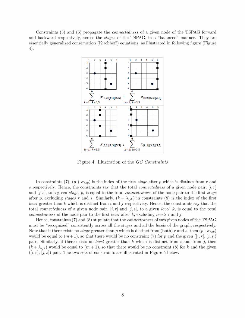
Constraints (5) and (6) propagate the connectedness of a given node of the TSPAG forwardand backward respectively, across the stages of the TSPAG, in a “balanced” manner. They areessentially generalized conservation (Kirchhoff) equations, as illustrated in following figure (Figure4).
Figure 4: Illustration of the GC Constraints
In constraints (7), (p+ σrsp) is the index of the first stage after p which is distinct from r ands respectively. Hence, the constraints say that the total connectedness of a given node pair, [i, r]and [j, s], to a given stage, p, is equal to the total connectedness of the node pair to the first stageafter p, excluding stages r and s. Similarly, (k + λijk) in constraints (8) is the index of the firstlevel greater than k which is distinct from i and j respectively. Hence, the constraints say that thetotal connectedness of a given node pair, [i, r] and [j, s], to a given level, k, is equal to the totalconnectedness of the node pair to the first level after k, excluding levels i and j.
Hence, constraints (7) and (8) stipulate that the connectedness of two given nodes of the TSPAGmust be “recognized” consistently across all the stages and all the levels of the graph, respectively.Note that if there exists no stage greater than p which is distinct from (both) r and s, then (p+σrsp)would be equal to (m+ 1), so that there would be no constraint (7) for p and the given ([i, r], [j, s])pair. Similarly, if there exists no level greater than k which is distinct from i and from j, then(k + λijk) would be equal to (m+ 1), so that there would be no constraint (8) for k and the given([i, r], [j, s]) pair. The two sets of constraints are illustrated in Figure 5 below.
8

Figure 5: Illustration of the CC Constraints
The IZ Constraints (9) serve a dual purpose. They ensure that the connectedness among thenodes in a given triplet is modeled by a unique x-variable. They also preclude the self-connectednessof a node being “built into” a given x-variable. Finally, (10)-(11) are the usual nonnegativityconstraints on the modeling variables.
3.2.2 Visualization of the model structure
For the short discussion to follow, refer to the solution illustrated in Figure 2. Constraints (1) and(2) represent the level/stage assignment problem abstraction of TSP tours (i.e., the so-called travel-times TSP polytope; see Diaby, Karwan, and Sun (2018)). We will label the nodes with positiveassignments (i.e., corresponding to nodes [i, r] ∈ N with w[i,r] > 0) in our example as “open.”
Now consider constraints (3) and (4). Fixing an open [i, r] (say, [5, 1]), leads to a unimodularstructure saying that there must exist positive values of connectedness to each of the other levelsand stages (excluding level 5 and stage 1). Having w[5,1] > 0 can be thought of as representinga colored (say, grey) “thread,” “rooted” in node [5, 1] which needs to be “weaved” through thegraph to cover every level and every stage. Of course, at this point we will have multiple coloredthreads rooted in our open [i, r] nodes corresponding to each positive w[i,r]. Note that if w[i,r] = 0,all corresponding x’s are zero and no thread rooted at [i, r] exists.
Constraints (5) and (6) say that the thread rooted in node [i, r] must branch to the end and thebeginning stages of the assignment graph. That is, each color/thread must reach out/be weavedon forward and backward to the end and the beginning stages of the graph, respectively.
Constraints (7) and (8) have a unimodular structure in (k, p) ∈ (L, S), given fixed nodes [i, r]and [j, s]. That is, open nodes “span” the levels and stages of the graph in pairs, for a third nodewith which to have connectedness. Hence, the constraints can be thought of as saying that every
9

color of thread must have the same “color intensity” (shade of grey, in the case of [5, 1]) at allstages and all levels of the assignment graph, respectively. Now, we can say that the threads are‘balanced’ across all levels and stages so that each colored thread must correspond to a TSP path.
3.2.3 Integrality of the model
We will now develop our formal proof-of-integrality.
Notation 10
1. Q :=
{(w
x
)∈ Rm2+m6
:
(w
x
)satisfies (1)− (11)
}.
2. W :={w ∈ Rm2
: w satisfies (1)− (2), (10)}.
3. W ′ :=
{w ∈ Rm2
:
(∃x ∈ Rm6
:
((w
x
)∈ Q
))}.
4. ∀w ∈W, X(w) :=
{x ∈ Rm6
:
((w
x
)satisfies (3)− (9), (11)
)}.
5. ∀(w
x
)∈ Q, define:
(a) Pw :={w[i,r], [i, r] ∈ N : w[i,r] > 0
};
(b) Px :={x[i,r][j,p][k,q], ([i, r], [j, p], [k, q]) ∈ N3 : x[i,r][j,p][k,q] > 0
}.
Remark 11
1. W is the Linear Assignment Problem (LAP) polytope (see Burkard et al. (2009)).
2. W ′ = W. (i.e., Q is an extended formulation of W .)
3. Q =
{(w
x
)∈ Rm2+m6
: w ∈W ; x ∈ X(w)
}.
4. There is a one-to-one correspondence between TSP paths of the TSPAG and extreme pointsof W .
5. There is a one-to-one correspondence between TSP tours and extreme points of W .
6. There is a one-to-one correspondence between extreme points of W and integral points of Q.
7. Each integral point of Q is an extreme-point of Q.
8. There is a one-to-one correspondence between TSP tours and integral points of Q.
Theorem 12 Q is integral, with a one-to-one correspondence between its extreme points and TSPtours.
10

Proof. Consider
(w
x
)∈ Q. The proof uses the fact that each extreme-point solution of W
has a special “staggered” structure over the TSPAG (i.e., with exactly one positive component foreach level and each stage of the TSPAG respectively). The idea is to show that the set of positive
components of
(w
x
)is comprised of (possibly-overlapping) subsets each of which has this special
extreme-point “staggered” structure, leading to the conclusion that
(w
x
)must have a convex
combination representation in terms of points which are in one-to-one correspondence with theextreme points of W . This is developed below.
1. Constraints (1)− (2), (10) =⇒(Pw :=
{w[i,r], [i, r] ∈ N : w[i,r] > 0
}6= ∅
). (12)
(In other words, the set of positive w-variables in a feasible solution must be non-empty.)
From Remarks 11.1 − 11.3, w must have at least one convex combination representation interms of extreme-point solutions of W . Let νw be the number of such representations whichare non-degenerate (i.e., with each of the extreme points used in the representation havinga positive weight in the representation). Let ∆k(w) denote the number of extreme points ofW used in the kth (k ∈ {1, . . . , νw}) representation. Then, Pw can be re-written as:
Pw =⋃νw
k=1
⋃∆k(w)
t=1
(Lk,tw
), (13)
where:
∀k ∈{1, . . . , νw} , ∀t ∈ {1, . . . ,∆k(w)} ,
Lk,tw : ={w
[uk,tr ,r]∈ Pw, r = 1, . . . ,m :
(∀(r, s) ∈ R2 : r 6= s, uk,tr 6= uk,ts
)}(14)
6= ∅, (15)
and the characteristic vector of each Lk,tw (t ∈ {1, . . . ,∆k(w)}) in w-variable space is anextreme-point solution of W, and hence (by Remarks 11.4−11.5), corresponds to exactly oneTSP Path of the TSPAG, and to exactly one TSP tour.
The above discussions are illustrated in Figure 6. The remainder of the proof consists essen-tially of showing that Px can be resolved into a similar “structure.”
2. We will now show that Px is comprised of subsets, each of which corresponds to exactly onemember of Pw. For the sake of brevity and simplifying the exposition, the non-negativityconstraints (10) and (11) will be implicitly assumed (and will not, therefore, be explicityreferenced) in the remainder of this discussion.
(a) Constraints (3)− (4) =⇒
∀[i, j] ∈ N,(w[i,j] > 0 iff ∃ ([j, p], [k, q]) ∈ N2 : x ([i, r][j, p][k, q]) > 0
). (16)
11

(b) The non-emptiness of Pw (Condition (12)) implies that there must exist nodes [i, r]’ssuch that w[i,r] > 0. Also, from condition (16) we have that for each [i, r] with w[i,r] > 0and each stage pair (p, q) (p 6= q), there must exist at least one node pair ([j, p], [k, q])such that x ([i, r], [j, p], [k, q]) is greater than zero.
For each x ([i, r], [j, p], [k, q]) which is greater than zero, constraints (5) − (6) induce(possibly-overlapping) sets of positive x-variables, each of which (sets) corresponds toexactly one stage set-spanning path of the TSPAG. Hence, for each [i, r] ∈ N suchthat w[i,r] > 0, there must exist a collection of sets of positive x-variables (induced byconstraints (5)−(6)) with each set corresponding to exactly one stage set-spanning pathof the TSPAG. Let Qx([i, r]) denote this collection of sets for a given [i, r] ∈ N whichis such that w[i,r] > 0. Then, Qx([i, r]) can be expressed as:
Qx([i, r]) =⋃πx([i,r])
t=1Ltx([i, r]),
where:
∀t ∈ {1, . . ., πx([i, r])},
Ltx([i, r]) :={x([i, r], [utp−1, p− 1], [utp, p]
)∈ Px,
(p = 2, . . . ,m; p /∈ {r, r + 1})} (17)
6=∅. (18)
(πx([i, r]) is the number of paths obtained from constraints (5) and (6) which force abranching out to the beginning and end of the TSPAG.)
Since the members of Px must satisfy constraints (5) − (6), each member of Px mustalso be a member of at least one Ltx([i, r]) ([i, r] ∈ N ; t ∈ {1, . . . , πx([i, r])}).In other words, we must have:
Px ⊆⋃
[i,r]∈N : w[i,r]>0Qx([i, r]). (19)
By definition ((17) above), each Ltx([i, r]) ⊆ Px. Hence, the following is true:
Px ⊇⋃
[i,r]∈N : w[i,r]>0Qx([i, r]). (20)
Combining (19) and (20) gives:
Px =⋃
[i,r]∈N : w[i,r]>0Qx([i, r])
=⋃
[i,r]∈N : w[i,r]>0
⋃πx([i,r])
t=1Ltx([i, r]) (21)
=⋃
[i,r]∈N : w[i,r]>0
⋃πx([i,r])
t=1
{x([i, r], [utp−1, p− 1], [utp, p]
)∈ Px,
(p = 2, . . . ,m; p /∈ {r, r + 1})} . (22)
12

(c) Suppose that for a given ([i, r], [j, s]) ∈ N2, there exists [k, p] ∈ N such that x([i, r], [j, s], [k, p]) >0. Then, constraints (7) induce a set of positive x-variables involving [i, r] and [j, s])and nodes at each of the other stages of the TSPAG.
Applying constraints (7) for each of the ([utp−1, p− 1], [utp, p]) pairs of (22), (22) can bere-written as:
Px =⋃πx
t=1Ltx (23)
where:
πx ∈ N+, with
max[i,r]∈N {πx([i, r])} ≤ πx <∑
[i,r]∈N : w[i,r]>0πx([i, r]); and (24)
∀t ∈ {1, . . . , πx} , Ltx :=
{(x([utp−1, p− 1], [utp, p], [u
tq, q]
)∈ Px,
(p = 2, . . . ,m; q = 1, . . . ,m : q /∈ {p− 1, p})} . (25)
(The value of πx depends on the number of conceptually overlapping paths.)
(d) From constraints (8) we have that:
∀([i, ri], [j, rj ]) ∈ N2, (∀u ∈ L, ∃ru ∈ R : x ([i, ri], [j, rj ], [u, ru]) > 0
iff ∀v ∈ L\{i, j, u},∃rv ∈ R : x ([i, ri], [j, rj ], [v, rv]) > 0) . (26)
(In words, constraints (8) stipulate that if ([i, ri] and [j, rj ]) are connected as a pair toone level of the TSPAG, they must be connected as a pair to all levels of the TSPAG.)
(e) From constraints (9),we have that:
∀ ([i, r], [j, s], [k, p]) ∈ N3, (x ([i, r], [j, s], [k, p]) > 0 =⇒ i 6= j 6= k) . (27)
(f) Applying constraints (7) to each ([utp, p], [utq, q]) pair in expression (25), and using (26)-
(27), (25) can be re-expressed as:
∀t ∈{1, . . . , πx} ,
Ltx ={x([utr, r], [u
tp, p], [u
tq, q]
)∈ Px, (r, p, q = 1, . . . ,m : r 6= p 6= q)
}(28)
={x([utr, r], [u
tp, p], [u
tq, q]
)∈ Px, (r, p, q = 1, . . . ,m : (r 6= p 6= q;
utr 6= utp 6= utq))}
. (29)
(The pair ([utp, p], [utq, q]) must be connected to all levels according to (26), since it is
connected to [utp−1, p − 1] (according to (25)). It must also be connected to all stagesaccording to (7).)
13

3. Using (16), Ltx (t ∈ {1, . . . , πx}) can be equivalently expressed as:
Lt
x,w :={(x([utr, r], [u
tp, p], [u
tq, q]
), w[utr,r]
, w[utp,p], w[utq ,q]
)∈ (Px, Pw, Pw, Pw) ,(
r, p, q = 1, . . . ,m :(r 6= p 6= q; utr 6= utp 6= utq
))}, (30)
with the following conditions holding:
∀t ∈ {1, . . . , πx} ,(x([utr, r], [u
tp, p], [u
tq, q]
), w[utr,r]
, w[utp,p], w[utq ,q]
)∈ L
t
x,w iff(x([utr, r], [u
tp, p], [u
tq, q]
)∈ Ltx; and
∃(
(k1, k2, k3) ∈ {1, . . . , νw}3 ; (t1, t2, t3) ∈ (∆k1(w), ∆k2(w), ∆k3(w)))
:
(w[utr,r], w[utp,p]
, w[utq ,q]) ∈ (Lk1,t1w , Lk2,t2w , Lk3,t3w )
). (31)
Hence, the set of positive components of
(w
x
)resolves into (possibly-overlapping) subsets,
each corresponding to exactly one Lk,tw (k ∈ {1, . . . , νw}; t ∈ {1, . . . ,∆k(w)}), and hence, toan extreme-point of W , and (using Remark 11.5) to a TSP tour.
Let
(wt
xt
)denote the characteristic vector of L
t
x,w (t ∈ {1, . . . , πx}). By (31) and also using
the IZ constraints (9), we have that
(wt
xt
)must be a feasible point of Q. Hence, by Remark
11.7 (since
(wt
xt
)is integral), each
(wt
xt
)(t ∈ {1, . . . , πx}) must be an extreme point of Q.
(13), (23), (30), and (31) (together) imply that each positive component of
(w
x
)is covered by
at least one
(wt
xt
)(t ∈ {1, . . . , πx}) (i.e., there is at least one characteristeric vector/extreme
point which has a “1” in its entry corresponding to the component of
(w
x
)). Hence, we
must have that
(w
x
)is a convex combination of the
(wt
xt
)′s (t ∈ {1, . . . , πx}). The theorem
follows directly from the combination of this, Remark 11.8, the arbitrariness of
(w
x
), and
the Minkowski-Weyl Theorem (Minskowski (1910); Weyl (1935); see also Rockafellar (1997,pp.153-172)) which states that a polytope may be represented by its faces or its vertices.
14

Figure 6: Illustration of Part 1 of the Proof of Theorem 12
3.3 Model objective
A wide variety of alternatives exists for developing an objective function to be optimized over Q,along the lines discussed in Diaby and Karwan (2016; pp. 85-90). The cost function we use in thispaper is shown in the following theorem.
Theorem 13 Let c ∈ R6 be a vector of costs indexed by nodes-triplets of the TSPAG and withcomponents derived from the TSP travel costs as follows:
∀([i, p], [j, r], [k, s]) ∈ N3,
c[i,p][j,r][k,s] :=
c0i + cij + cjk if (p = 1; r = 2; s = 3);
cjk + ck0 if (p = 1; r = m− 1; s = m);
cjk If (p = 1; 3 ≤ r ≤ m− 2; s = r + 1);
0 Otherwise.
(32)
15

Then, the linear program (Problem TSPLP) below:∣∣∣∣∣∣∣∣∣∣∣∣∣∣∣∣∣∣
Minimize :
V((
w
x
)):=(0T , cT
)·(w
x
)=
m∑i,r,j,s,k,p=1
c[i,r][j,s][k,p]x[i,r][j,s][k,p]
Subject to:(w
x
)∈ Q
correctly solves the TSP.
Proof. Since the extreme points of Q are in one-to-one correspondence with TSP tours (ac-cording to Theorem 12), it is sufficient to show that the cost associated to an extreme point of Q isequal to the cost of the corresponding TSP tour. We will do this by a “direct counting” approach.
Let
(w
x
)be an extreme point of Q. Then, using (28) and the IZ constraints (9), there must
exist a (unique) set {ip ∈ L, p = 1, . . . ,m} such that:
∀(p, r, s) ∈ R3, x[ip,p][ir,r][is,s] =
1 if p < r < s;
0 otherwise.(33)
The corresponding TSP tour is 0→ i1 → . . .→ im → 0. Let “TCost” denote the cost of this tour.Then, we have:
TCost = c0,i1 + cim,0 +m−1∑q=1
ciq ,iq+1 . (34)
Now, consider V((
w
x
)). Using (32) and (33), we have the following:
Case x-component Cost
p = 1; r = 2; s = 3 c0,i1 + ci1,i2 + ci2,i3p = 1; r = m− 1; s = m cim−1,im + cim,0p = 1; r = 3; s = 4 ci3,i4...
...
p = 1; r = m− 2; s = m− 1 cim−2,im−1
Total Cost, V((
w
x
))= c0,i1 + cim,0 +
m−1∑q=1
ciq ,iq+1
Comparing the results of the enumeration above for the components of x to (34), we observethat V (·) of Problem TSPLP correctly captures TSP tour costs.
16

3.4 Computational complexity order of the model size
The following theorem establishes the polynomial size of the model.
Theorem 14
1. The computational complexity order of the number of non-implicitly-zero variables in thesystem (1)− (11) is O(n6).
2. The computational complexity order of the number of constraints which must be explicitlyexpressed in a linear programming (LP) optimization problem over the system (1)− (11) isO(n5).
Proof.
1. The possible total number of variables in the system (1) − (11) is equal to (m6 + m2), andthe number of implicitly-zero variables in the system is greater than zero. Hence, letting nvdenote the number of non-implicitly-zero variables in the system, we must have:
nv < m6 +m2 < 2m6 = 2(n− 1)6. (35)
Hence, nv is bounded by a 6th-degree polynomial function of n. Part (1) of the theoremfollows from this directly.
2. Consider the classes/types of constraints which must be explicitly stated in an LP over thesystem (1)− (11). We have:
Constraint Bound onClass/Type Total Count
LAP 2m
IC 2m3
GC 2m4
CC 2m5
Hence, letting nc denote the number of constraints which must be explicitly expressed in anLP over the system, we must have:
nc < 2(m5 +m4 +m3 +m) < 8m5 = 8(n− 1)5 (36)
Hence, nc is bounded by a 5th-degree polynomial function of n. Part (2) of the theoremfollows from this directly.
4 Some immediate extensions
In this section, we will discuss some extensions of our proposed model to some other well-studiedproblems. The extensions do not require any modifications to the constraints set ((1) − (11)) ofour model. Hence, we refer to them as “immediate extensions.” The proofs-of-correctness for theobjective functions that we apply for these extensions are similar to that of Theorem 13 and willtherefore be omitted.
17

4.1 Time-dependent traveling salesman problem (TDTSP)
As indicated earlier, reviews of TDTSPs can be found in Gouveia and Voss (1992), Abeledo etal. (2013), Godinho et al. (2014), and Gendreau et al. (2015). In this section, we will considerthe commonly-used form which was first introduced in the seminal Picard and Queyranne (1978)paper, and in which inter-city travel costs also depend on the times-of-travel.
Denote by dirj the cost incurred when cities i and j are visited at times r and r+1, respectively.Let d0i be the travel cost from city “0” to city i, and di0, the cost of travel from city i to city “0.”Then, the extension of our proposed LP model to the TDTSP consists of applying the objectivefunction resulting from the costs below over the constraints set defined by (1)− (11) (i.e., Q):
∀([i, p], [j, r], [k, s]) ∈ N3,
d[i,p][j,r][k,s] :=
d0i + dipj + djrk if (p = 1; r = 2; s = 3);
djrk + dk0 if (p = 1; r = m− 1; s = m);
djrk If (p = 1; 3 ≤ r ≤ m− 2; s = r + 1);
0 Otherwise.
(37)
4.2 Quadratic assignment problems
The quadratic assignment problem (QAP) is different from the LAP only in that its objectivefunction consists of minimizing the sum of assignment interaction costs, plus fixed costs for theindividual assignments. The QAP is one the most-extensively studied problems in operationsresearch. The two best-recognized seminal papers are those by Koopmans and Beckmann (1957)and Lawler (1963), respectively. NP-hardness was established in the 1970’s (Sahni and Gonzales(1976)). Reviews can be found in Pardalos et al. (1994), Cela (1998), Anstreicher (2003), Loiolaet al. (2007), and Hahn et al. (2010), among others.
By letting L and S in Notations 7 .4-7.5 stand for the two sets of objects to be assigned to eachother, QAP and many of its variants can be solved as LPs over Q. We generically consider thatthere is a fixed cost, oir, which is incurred when i ∈ L is assigned to r ∈ S, and that an interactioncost, hirjs, is incurred when i, j ∈ L are assigned to r, s ∈ S, respectively. The objective is to findan assignment which minimizes the total of these costs.
18

4.2.1 Generalized quadratic assignment problem (GQAP)
In the GQAP, the assignment interaction costs (the hirjs’s) are arbitrary (see Hahn et al. (2010)).For this problem, the costs to attach to our x-variables are as shown in (38) below:
∀([i, p], [j, r], [k, s]) ∈ N3,
h[i,p][j,r][k,s] :=
oip + hipjr + hipks if (r = p+ 1; r + 1 = s < m);
oip + ojr + oks + hipjr + hipks + hjrks
if (r = p+ 1; r + 1 = s = m);
hipks If (r = p+ 1; r + 1 < s);
0 Otherwise.
(38)
4.2.2 “Standard” quadratic assignment problem (QAP)
In a facilities location/allocation context where the objective is to minimize the generic materialhandling costs (see Koopmans and Bechmanns (1957)), the GQAP reduces to the “standard”QAP. In this case, let L and S stand for the sets of “departments” and “sites,” respectively. Letfij ((i, j) ∈ L2 : i 6= j) denote the flow volume from department i to department j, and drs((r, s) ∈ S2 : r 6= s), the cost of movement from site r to site s. Then, the interaction costs aredecomposable, and (38) can be re-expressed using the following:
∀(i, j) ∈ L2 : i 6= j, ∀(r, s) ∈ S2 : r 6= s,
hirjs = fijdrs + fjidsr. (39)
4.2.3 Cubic assignment problem (CAP)
The CAP is an extension of the GQAP in which the interaction costs involve triplets (instead ofdoublets) of assignments (see Hahn et al. (2010)). Let the interaction cost of assigning i, j, k ∈ Lto p, r, s ∈ S respectively, be denoted as eipjrks. The objective function to attach to our x-variablesare h[i,p][j,r][k,s] = eipjrks for all ([i, p], [j, r], [k, s]) ∈ N3.
4.2.4 Relation to relaxation-linearization-technique (R-L-T) models
Our proposed model has some similarity with the R-L-T models (Adams and Sherali (1986); Sheraliand Adams (1999); Adams et al. (2007); Hahn et al. (2012)). In fact, the modeling variables inthis paper are essentially the same as the 6-indices variables of the Level-2 R-L-T model whichcorrespond to triplets of assignments (Adams et al. (2007)). However, all of the constraints andadditional variables of the Level-2 R-L-T model are redundant for our constraints set ((1)− (11);Q). Hence, our proposed LP model strictly subsumes the continuous relaxation of the Level-2R-L-T model. In general, for a m-assignment QAP, the model proposed in this paper is equivalentto the Level-(m− 1) R-L-T model only.
19

5 Numerical experimentation
As shown in section 3.4 above, the numbers of variables and constraints of our proposed model areO(n6) and O(n5), respectively. In order to get a sense of the actual size and the computationalperformance of the model (although we are aware that streamlined or large-scale optimizationapproaches will have to be eventually developed for the model to be useful in practice), we undertooda C# implementation of it (see the Appendix of this paper) and applied it to randomly-generatedproblems as well as some “test bank” problems from the literature.
For the purpose of assessing the actual model size, we ran “counting procedures” in our codefor TSPs with 7 to 25 cities. These runs were done on a Dell Precision T7610 workstation withdual-Intel Xeon E5-2605v2 processors (2.50 GHz each) and 512 GB of RAM. The results of theseruns are shown in Table 1.
Number of Number of Number ofCities Variables Constraints
7 2,436 3,792
8 7,399 9,380
9 18,880 20,064
10 42,417 38,682
11 86,500 68,960
12 163,471 115,632
13 290,544 184,560
14 490,945 282,854
15 795,172 418,992
16 1,242,375 602,940
17 1,881,856 846,272
18 2,774,689 1,162,290
19 3,995,460 1,566,144
20 5,634,127 2,074,952
21 7,798,000 2,707,920
22 10,613,841 3,486,462
23 14,230,084 4,434,320
24 18,819,175 5,577,684
25 24,580,032 6,945,312
Table 1: TSP LP Size vs. Number of TSP Cities
We performed some regression on the results summarized in Table 1 above. The best fitswe obtained are shown in Figure 7. While the complexity order of the number of variables andconstraints of the model are O(n6) and O(n5) respectively (Theorem 14), the regressions appear tosuggest actual (“practical”) size orders of O(n4) and O(n3), respectively. These lower “practical”numbers are likely due to the many implicitly-zero variables in the model. We note that the factthat the number of constraints grows more slowly than the number of variables suggests that theremay be an advantage to focusing on the primal problem in efforts aimed at developing streamlinedsimplex procedures for solving the model.
In solving our test problems, we used the “barrier method with no crossover” implementationof CPLEX 12.8, on a Dell OptiPlex 7050 MT computer with an Intel i7-7700 (3.6 GHz) processor
20

and 64 GB of RAM. The correctness of the LP optima were verified using common/traditional in-teger programming TSP and QAP formulations and solving these using the branch-and-bound/cutprocedures of CPLEX 12.8. The randomly-generated problems were for the TSP only. They werebased on symmetric Euclidean distances. The cities were generated on a 100 by 100 grid and theEuclidian distances between them were modified by factors between 80%-120% and rounded to beintegers. The largest problems we could solve under 60 hours of CPU time were 14-city problems.The results for these are summarized in Table 2. Each of the times shown in this table is theaverage of five (5) problems. Similar results were obtained using exact Euclidean distances, usinguniform distributions for distances, and choices of symmetric/asymmetric/integer or non-integervalues.
Figure 7: Number of Variables and Constraints vs. Number of TSP Cities
Number CPU Timeof Cities Seconds Minutes
7 0.80 0.01
8 8.55 0.14
9 59.32 0.99
10 334.58 5.58
11 1,809.67 30.16
12 8,842.49 147.37
13 35,025.67 583.76
14 191,044.23 3,184.07
Table 2: Computational Times vs. Number of TSP Cities
21

H]
Figure 8: CPU Minutes vs. Number of TSP Cities
The regression we performed on the computational times in Table 2 are summarized in Figure8. The fact that these times can be “well-fitted” by a polynomial function (of the number of cities)is consistent with the fact that both the size of our LP model and the complexity of the the solutionmethod we used are polynomial. The “practical” CPU time order which seems to be suggestedby this regression is O(n5). We recall, as we indicated earlier in this section, that streamlined,large-scale-optimization, or efficient distributed-computing procedures for solving our proposed LPwill need to be developed eventually, in order for the model to be useful in practice.
With respect to the “testbank” problems, we solved all of the TSP instances of the SMAPOLibrary (Reinelt (2010)). These involved 15,379 10 -city problems, 192 9 -city problems, 24 8 -cityproblems, 6 7 -city problems, and 4 6 -city problems. We also solved the smallest (12 -department)QAPs from the QAPLIB Library (Anjos (2018)), namely, Problems “Chr12a,” “Chr12b,” “Chr12c,”“Had12,” “Nug12,” “Rou12,” “Scr12,” “Tai112a,” and “Tai12b”. Our results for all of these (TSPand QAP) problems were similar to those for our randomly-generated problems, consistently withour expectations, based on our theoretical developments.
6 Conclusions
We have presented an exact extended formulation of the assignment problem polytope which solvesthe TSP and QAP as polynomial-sized linear programs (LPs). The model is an analog of theprevious models developed by the first two authors of this paper. However, it is much smaller andits proof is much simpler. Hence, we believe it represents a very significant improvement over those
22

previous models. Our work complements our earlier affirmations resolving the important “P versusNP” question.
To paraphrase/quote from Diaby and Karwan (2016, pp. 5-7):
‘Our developments (and their incidental consequence of “P = NP”) remove theexponential shift in complexity, but do not suggest a collapse of the “continuum ofdifficulty,” nor any change in the sequence along that continuum. In other words, ourdevelopments do not imply (or suggest) that all of the problems in the NP class havebecome equally “easy” to solve in practice. The suggestion is that, in theory, for NPproblems, the “continuum of difficulty” actually ranges from low-degree-polynomialtime complexity to increasingly-higher-degree-polynomial time complexities.
However, from a theoretical perspective, we believe that these results make it neces-sary to reframe the computational complexity question away from: “Does there exist apolynomial algorithm for Problem X ?” to (perhaps): “What is the smallest-dimensionalspace in which Problem X has a polynomial algorithm”’
In other words, since our work shows that every decidable problem which is solvable in polyno-mial time by a nondeterministic computer (i.e., every problem in the NP class) is tractable, focusof Complexity Theory for class-NP problems should be shifted to a new paradigm for “problemdifficulty.” For example, Garey and Johnson (1979, p. 13) write:
‘As theoreticians continue to seek more powerful methods for proving problemsintractable, parallel efforts focus on learning more about the ways in which variousproblems are interrelated with respect to their difficulty. As we suggested earlier, thediscovery of such relationships between problems often can provide information usefulfor algorithm designers.’
Our suggestion is that, perhaps, the new paradigm could be a continuation or re-direction ofcurrent Complexity Theory in which classifications would not be independent of possible alternateencodings (or roughtly, “modeling”) of a problem.
23

References
[1] Abeledo, H., R. Fukasawa, A. Pessoa, and E. Uchoa (2013). The time-dependent travelingsalesman problem: polyhedra and algorithm. Mathematical Programming Computation 5:1, pp.27-55.
[2] Adams, W.P., and H.D. Sherali (1986). A tight linearization and an algorithm for zero-onequadratic programming problems. Management Science 32:10, 1274–1290.
[3] Adams, W.P., M. Guignard, P.M. Hahn, and W.L. Hightower (2007). A level-2 reformulation–linearization technique bound for the quadratic assignment problem. European Journal of Op-erational Research 180:3, pp. 983-996.
[4] Anjos, M. (2018). QAPLIB Problem Instances and Solutions. Online:http://anjos.mgi.polymtl.ca/qaplib/inst.html#BO.
[5] Kurt M. Anstreicher, K.M. (2003). Recent advances in the solution of quadratic assignmentproblems. Mathematical Programming 97:1–2, pp 27–42.
[6] Applegate D, Bixby R, Chvatal V, Cook W (2007). The traveling salesman problem: a compu-tational study. Princeton series in applied mathematics. Princeton University Press, Princeton
[7] Balas, E. and P. Toth (1985). Branch and bound methods. In: Lawler E, Lenstra J, RinnooyKan A, Shmoys D. (eds) The Traveling Salesman Problem: a guided tour of combinatorialoptimization. Wiley, New York, pp 361–401.
[8] Bazaraa, M.S., J.J. Jarvis and H.D. Sherali (2010). Linear Programming and Network Flows.Wiley, New York, NY.
[9] Burkard, R., M. Dell’Amico, and S. Martello (2009). Assignment Problems. SIAM (Philadel-phia).
[10] Cela, E. (1998). The quadratic assignment problem: theory and algorithms. Kluwer Aca-demicPublishers (London).
[11] D’Ambrosio C, Lodi A, Martello S (2010). Combinatorial traveling salesman problem algo-rithms. In: Wiley encyclopedia of operations research and management science, vol 1. Wiley,New York, pp 738–747.
[12] Diaby, M. (2007). The traveling salesman problem: A linear programming formulation.WSEAS Transactions on Mathematics 6:6, pp. 745–754.
[13] Diaby, M. (2010a). Linear programming formulation of the multi-depot multiple travelingsalesman problem with differentiated travel costs. In D. Davendra (ed.), Traveling SalesmanProblem, Theory and Applications. InTech, New York, NY, pp. 257–282.
[14] Diaby, M. (2010b). Linear programming formulation of the set partitioning problem. Interna-tional Journal of Operational Research 8:4, pp. 399–427.
[15] Diaby, M. (2010c). Linear programming formulation of the vertex coloring problem. Interna-tional Journal of Mathematics in Operational Research 2:3, pp. 259–289.
24

[16] Diaby, M. and M.H. Karwan (2016). Advances in Combinatorial Optimization: Linear Pro-gramming Formulations of the Traveling Salesman and Other Hard Combinatorial OptimizationProblems. World Scientific Publishing, Singapore.
[17] Diaby, M. and M.H. Karwan (2017). Limits to the scope of applicability of extended formu-lations theory for LP models of combinatorial optimisation problems. International Journal ofMathematics in Operational Research 10:1, pp. 18-33.
[18] Diaby, M., M.H. Karwan, and L. Sun (2016). A Small-Order-Polynomial-Sized Lin-ear Program for Solving the Traveling Salesman Problem. Unpublished (Available at:https://arxiv.org/abs/1610.00353).
[19] Diaby, M., M.H. Karwan, and L. Sun (2018). On modeling hard combinatorial optimizationproblems as linear programs: Refutations of the “unconditional impossibility” claims. Interna-tional Journal of Operational Research (Forthcoming).
[20] Fiorini, S., S. Massar, S. Pokutta, H.R. Tiwary, and R. de Wolf (2011). Linear vs. SemidefiniteExtended Formulations: Exponential Separation and Strong Bounds. Unpublished (Availableat: http://arxiv.org/pdf/1111.0837.pdf).
[21] Fiorini, S., S. Massar, S. Pokutta, H.R. Tiwary, and R. de Wolf (2012). Linear vs. SemidefiniteExtended Formulations: Exponential Separation and Strong Bounds. Proceedings of the 44 th
ACM Symposium on the Theory of Computing (STOC ’12 ), New York, NY, pp. 95-106.
[22] Fiorini, S., S. Massar, S. Pokutta, H.R. Tiwary, and R. de Wolf (2015). Exponential LowerBounds for Polytopes in Combinatorial Optimization. Journal of the ACM 62:2, Article No.17.
[23] Fischetti M, Lodi A, Toth P (2002). Exact methods for the asymmetric traveling salesmanproblem. In: Gutin G, Punnen A (eds) The traveling salesman problem and its variations.Kluwer Academic Publishers, The Netherlands, pp 169–205.
[24] Furini, F., C.A. Persiani, and P. Toth (2016). The time-dependent traveling salesman planningproblem in controlled airspace. Transportation Research Part B 90 (August), pp. 38-55.
[25] Garey, M.R. and D.S. Johnson (1979). Computers and Intractability: A Guide to the Theoryof NP-Completeness. Freeman and Company, New York, NY.
[26] Gendreau, M., G. Ghiani, E. Guerriero (2015). Time-dependent routing problems: A review.Computers & Operations Research 64 (December), pp. 189-197.
[27] Godinho, M.T., L. Gouveia, P. Pesneau (2011). On a time-dependent formulation and anupdated classification of ATSP formulations. In Mahjoub, A.R. (ed.) Progress in CombinatorialOptimization (Chapter 7, pp. 223-252). Wiley, New York.
[28] Godinho, M.T., L. Gouveia, P. Pesneau (2014). Natural and extended formulations for thetime-dependent travelling salesman problem. Discrete Applied Mathematics 164 (Part 1; Febru-ary), pp. 138-153.
[29] Gouveia, L. and S. Voss (1995). A classification of formulations for the (time-dependent)traveling salesman problem. European Journal of Operational Research 83:1, pp. 69-82.
25

[30] Gutin G, Punnen A (2002) The traveling salesman problem and its variations. Kluwer,Dortrecht.
[31] Hahn, P.M., Y.-R. Zhu, M. Guignard, J.M. Smith (2010). Exact solution of emerging quadraticassignment problems. International Transactions in Operational Research 17:5, pp. 525-552.
[32] Hahn, P.M., Y.-R. Zhu, M. Guignard, W.L. Hightower, and M.J. Saltzman (2012). A Level-3Reformulation-Linearization Technique-Based Bound for the Quadratic Assignment Problem.INFORMS Journal on Computing 24:2, pp. 202-209.
[33] Koopmans, T.C., M.J. Beckmann (1957). Assignment problems and the location of economicactivities. Econometrica 25:1, pp. 53–76.
[34] Lawler,E.L. (1963). The quadratic assignment problem. ManagementScience 9:4, pp. 586–599.
[35] Lawler, E.L., J.K. Lenstra, A.H.G. Rinnooy Kan, and D.B. Shmoys (1985), eds. The TravelingSalesman Problem: A Guided Tour of Combinatorial Optimization (Wiley, New York).
[36] Loiola, E.M., N.M.M Abreu, P.O. Boaventura-Netto, P.M. Hahn, T. Querido (2007). A surveyfor the quadratic assignment problem. European Journal of Operational Research 176:2, pp.657–90.
[37] Miller, C.E., A.W. Tucker and R.A. Zemlin (1960). Integer programming formulations andtraveling salesman problems. Journal of the Association for Computing Machinery 7:4, pp.326–329.
[38] Minkowski, H. (1910). Geometrie der Zahlen. Teubner, Leipzig.
[39] Oncan, T., K. Altinel and G, Laporte (2009). A comparative analysis of several asymmetrictraveling salesman problem formulations. Computers & Operations Research 36:3, pp. 637–654.
[40] Padberg, M. and T.-Y. Sung (1991). An analytical comparison of different formulations of thetravelling salesman problem. Mathematical Programming 52, pp. 315-357.
[41] Pardalos, P.M. F. Rendl, and H. Wolkowicz (1994). The quadratic assignment problem: asurvey and recent developments. In P.M. Pardalos and H. Wolkowicz (eds.). Quadratic assigne-ment problems and related problems 16, pp. 1–42. DIMACS. American Mathematical Society(Providence, RI).
[42] Picard, J.C. and M. Queyranne (1978). The time-dependent traveling salesman problem andits application to the tardiness problem in one-machine scheduling. Operations Research 26, pp.86-110.
[43] Reinelt G. (1994). The traveling salesman problem: computational solutions for TSP applica-tions. Lecture Notes in Computer Science. Springer, Berlin.
[44] Reinelt G. (2010). SMAPO Library: Symmetric and Graphical Traveling Salesman polyhedra.Online: https://www.iwr.uni-heidelberg.de/groups/comopt/software/SMAPO/tsp/.
[45] Roberti, R. and P. Toth (2012). Models and algorithms for the asymmetric traveling salesmanproblem: an experimental comparison. EURO Journal on Transportation and Logistics 1:1-2,pp. 113-133.
26

[46] Rockaffelar, R. T. (1997). Convex Analysis. Princeton University Press.
[47] Sahni, S. and T. Gonzalez (1976). P-complete approximation problems. Journal of the Asso-ciation for Computing Machinery 23:3, pp. 555–565.
[48] Sherali, H.D., and W.P. Adams (1999). A Reformulation–Linearization Technique for SolvingDiscrete and Continuous Nonconvex Problems (1st edn). Kluwer Academic Publishers (Norwell,MA).
[49] Weyl, H. (1935). Elementare Theorie der konvexen Polyheder. Commentarii Math. Helvetici7, pp. 290-306.
[50] Wright, S.J. (1997). Primal-Dual Interior-Point Methods. SIAM.
[51] Yannakakis, M. (1991). Expressing combinatorial optimization problems by linear program-ming. Journal of Computer and System Sciences 43:3, pp. 441-466.
27

Appendix:Software Implementation
• General Description and Interface
A software package, “TSP/QAP LP Solver,” has been developed to implement the model inthis paper. The solver builds linear programming (LP) models for the traveling salesman andquadratic assignment problems and calls CPLEX 12.8 to solve them as LPs. The interface hasbeen designed to run multiple replications of the chosen problem and run control settings at a time.With this tool, users can: (1) randomly generate or read a TSP or QAP input data in multipleways; (2) directly solve the TSP or only build the LP models for them; (3) adjust CPLEX settingsfor different tests; (4) show solutions (optimal objective, variables, routes) in different formats.Standard integer programming (IP) models are incorporated and can be used for the purpose ofverifying the correctness of the solutions obtained using our LP model. These are solved as IPs,and only their objective function values are displayed. A screenshot of the solver is shown in Figure9 below.
Figure 9: First Screen of the TSP/QAP LP Solver
28

• Requirements
TSP/QAP LP Solver is written in C# with .NET Framework 4 and calls CPLEX 12.8 to solvethe TSP and QAP n6 LP models. For those with CPLEX 12.8, all functions in this program areavailable. Users who do not wish (or are not able) to use CPLEX 12.8 can choose the “ModelOnly” option in order to build .lp files for the LP or IP models, which they can then solve usingthe software of their choice. An advantage of solving the LP models endogeously is that it givesthe user an option to “parse” the LP solution in order to produce an an optimal TSP tour or QAPassignment, thus removing the burden of having to interprete the optimal values of the modeling(the w- and x-) variables from the user. This is especially useful when the barrier method withoutcrossover is used and it stops with a non-extreme-point, convex combination of alternate optimalsolutions.
• Data
There are two ways to input data to the solver. They may be randomly generated or they maybe read from files. For either way, users can check “Export all replications in XML format” toexport input data to files in XML format for every replication.
Randomly generating data supports the testing of multiple replications of a problem in a singlerun. Users input the number of cities (“# of Cities”) for the TSP or the number of departments (“#Depts/Sites”) for the QAP, and the number of replications (“# of Replications”) desired. For theTSP, cost values are generated based on either Euclidean distances or uniformly distributed randomnumbers. If the Euclidean distance option is chosen, the program will first randomly generatecoordinates within a (0, 100) x (0, 100) square plane, and then randomly generate costs within thegiven percentage range of Euclidean distances. If (absolute) interval limits is chosen, the programwill directly randomly generate costs within the given range, not based on Euclidean distances.Other options include whether the cost matrix is asymmetric or not (checked or unchecked), whetherthe cost matrix is integer or not (checked or unchecked), and whether the triangle inequality holdsor is not required (checked or unchecked). For the QAP, all the inter-departmental flows, inter-sitedistances, and fixed location assignment costs are generated from uniform distributions over theintervals specified by the user.
Reading input data files supports XML and CSV formats as input file formats for the TSP, andCSV format only for the QAP. The required data format can be found in the included Sample.xmland Sample.csv. The XML data format for the TSP follows that of the classic TSPLIB.
• Modelers and Solvers
– Modeler Settings
For the TSP, if the “Model Only” button is chosen, the program will build an .lp filewithout the requirement to use CPLEX. If the Miller-Tucker-Zemlin (MTZ) model ischosen to be solved, the program will call CPLEX to build and solve the MTZ IP modeland display the optimal objective value for reference. If the n6 TSP LP model is chosento be solved, the program will call CPLEX to build and solve the model and displaythe solution time, optimal objective value and other solution information depending onwhich among the “Show w solution,” “Show x solution,” and “Show an optimal route”options are chosen .
29

Similarly, for the QAP, if the “Model Only” button is chosen, the program will build an.lp file without the requirement to use CPLEX. If the standard QAP IP model is chosento be solved, the program will call CPLEX to build and solve the IP model for QAPand display the optimal objective value for reference. If the n6 QAP LP model is chosento be solved, the program will call CPLEX to build and solve the model and displaythe solution time, optimal objective value and other solution information dependingon which are chosen among the “Show w solution,” “Show x solution,” and “Show anoptimal assignment” options.
– CPLEX Settings
If users have the correct CPLEX version on their machines, they can adjust CPLEXparameters with this tool and solve the model with different algorithmic settings. Fordetails of each adjustable parameter, please refer to a CPLEX Parameters Referencefrom IBM.
• Results
All output files are located in the “Results/TSP” and “Results/QAP” subfolders of the foldercontaining the TSP/QAP LP Solver executable (“TSPsolvers.exe”), including the XML andCSV data files, .lp files, and solution text files.
We note that the “parser” that is incorporated in the software is only heuristic. It is not,therefore, guaranteed to succeed in “retrieving” a TSP tour or QAP assignment when thebarrier method without crossover stops with a non-extreme point solution. In such a case, theLP model will need to be re-solved either with primal simplex, dual simplex, or the barriermethod with crossover to primal or dual simplex, if an extreme-point (integral) solution isdesired. In our experimentation, the barrier method with dual crossover has consistentlybeen the most efficient method for such cases.
30