A single theory for some quasi-static, supersonic,atomic, and tectonic scale applications of dislocations

Xiaohan Zhang, Amit Acharya, Noel J. Walkington, Jacobo Bielak

July 8, 2015

Abstract

We describe a model based in continuum mechanics that reduces the study of a signifi-cant class of problems of discrete dislocation dynamics to questions of the modern the-ory of continuum plasticity. As applications, we explore the questions of the existenceof a Peierls stress in a continuum theory, dislocation annihilation, dislocation dissoci-ation, finite-speed-of-propagation effects of elastic waves vis-a-vis dynamic dislocationfields, supersonic dislocation motion, and short-slip duration in rupture dynamics.

1 Introduction

This paper explores some qualitative aspects of Field Dislocation Mechanics (FDM), a non-linear, partial differential equation (pde)-based model of the mechanics of dislocations. Thephysical phenomena explored correspond to behaviour of individual or a collection of fewdislocations. In particular, we analyse phenomena complementary to what can be dealt withby the Discrete Dislocation Dynamics methodology in a fundamental manner. Specifically,we explore

• Peierls’ stress effects in a translationally-invariant continuum theory like FDM.

• Dislocation annihilation and dissociation as consequences of fundamental kinematicsand energetics and not targeted constitutive rules for the phenomena.

• Dislocation dynamics in the presence of significant effects of material inertia, includingfinite-speed-of-propagation effects of elastic waves and dislocation motion past sonicspeeds.

• Dislocation dynamics with nonlinear elasticity.

• Short-slip duration in rupture dynamics.

The question of the possibility of a Peierls-like threshold for onset of dislocation motionin a translationally-invariant, time-dependent continuum theory was discussed in [Ach10].The classical, static, argument going back to Peierls [Pei40] relies crucially on the fact thatsuch a threshold is directly related to changes in the total potential energy of the body

1

induced by changes in position of the dislocation (naturally, then, viewed as a rigid objector profile). Since in a homogeneous infinite continuum the total potential energy remainsinvariant due to changes in position of the rigid dislocation profile, the conclusion is thatthere cannot be a Peierls stress in a translationally-invariant continuum theory; breakingtranslational invariance, possibly by modelling the effects of an atomic lattice (as was doneby Peierls [Pei40] and Nabarro [Nab47]) or by introducing a heterogeneous medium, canintroduce a Peierls stress. However, questions of stability of equilibria under perturbationsof loading in a time-dependent model of dislocation mechanics with a significantly differentnotion of a driving force (that includes self stress effects) can be quite different, in particularwhether an unloaded equilibrium dislocation profile can serve as a traveling wave profileunder a continuous spectrum of finite loads tending to zero - and, if not, is there an intervalof loads about zero for which different equilibrium profiles can be attained parametrized bythe load. Such questions have to do intimately with changes in ‘shape’ of the dislocationprofile. In this paper we computationally explore this question - as a point of principle,most of all - for three natural models that the structure of FDM makes available. Thesecorrespond to a non-local Ginzburg Landau model, a non-local level set model and whatmay be termed a generalized, non-local Burgers model. In Sections 4 and 7.1 we describethese models and results in detail. Despite the great utility of analysis of traveling waves,our results point definitely in the direction of avoiding an over-reliance on characteristicsof traveling wave solutions in making general statements about the non-existence of certaintypes of predictions related to the representation of physical phenomena characterized byfronts. After all, there is no reason why a traveling front necessarily has to be perfectly rigidduring motion, making an infinite-dimensional object (a profile allowed to change shape,while still remaining localized) into one of dimension 1. A physical example related to thispaper is the onset of motion of screw dislocations in some BCC materials. There, it isunderstood that the dislocation core is spread out on multiple planes and the core has tobe compacted further into a preferred slip plane before gross motion can ensue; once motionstops, the multiple-plane equilibrium configuration is regained. In a qualitative sense, wedemonstrate such features, including differences between dynamic and equilibrium shapes inSection 7.

With respect to dislocation annihilation, since the fundamental statement of evolutionin FDM is a conservation law for Burgers vector content of the dislocation density field,the density field evolves by tensorial addition rules resulting in natural accumulation orannihilation of non-singular localizations of net positive and negative Burgers vector whenphysically expected. We demonstrate such results in Section 7.4.

The discussion of the possible dissociation of a dislocation of a certain Burgers vectorstrength into two whose strengths vectorially sum up to that of the original one is a text-book example of the phenomenology of dislocations related to the energy-decreasing featureof dislocation mechanics. Due to the treatment of a dislocation core as either a formless or arigid singularity in classical versions of any sort of dislocation dynamics, dissociation cannotbe a prediction. The field setting is ideally suited for such explorations as we demonstratein Sec. 7.1.7.

As for dislocation dynamics with material inertia, it is physically natural that a movingdislocation induces elastic stress-waves that cannot transmit the stress signal instantaneouslyto all parts of the body. This fact is naturally encoded in FDM and our simulations, without

2

extra effort or computational expense beyond solving standard elastodynamics equations.As discussed in [GLBD+13], when time intervals of observation are small (as in very highrate deformations) this time delay in stress signal transmission due to stress-wave propaga-tion can be of importance, and merely correcting for individual dislocation motion laws inDD simulations by added-mass effects, while utilizing the static stress fields of dislocations,is not sufficient; instead, dislocation stress fields utilizing the full dynamic Green’s functionhave to be utilized and this becomes a significantly onerous task, especially with increasein number of segments. We demonstrate the efficacy of FDM in dealing with such prob-lems in Section 8.3. In addition, we show that there is no conceptual or practical problemwithin FDM in dealing with dislocation motion past linear-elastic sonic speeds (in appro-priate circumstances) as observed in the molecular dynamics (MD) experiments of [GG99],or in dealing with nonlinear elasticity, with beneficial effect related to matching trends ofdislocation velocity vs. applied loading to MD results.

Finally, we make a successful first attempt at modeling the observed phenomenon ofshort-slip duration in earthquake rupture as well as the more conventional crack-like slipresponse obtained from slip-weakening cohesive zone models of rupture dynamics. Thesefeatures are obtained without sophisticated constitutive modifications of velocity-weakeningor rate-and-state friction type, but simply by invoking a requirement of damage of elasticmodulus at a point on propagation of the rupture front past it.

In this work we utilize an ansatz to produce an exact, reduced, plane model of FDM.Our model is built on the previous work of [Ach10] where a 1-d FDM model was derivedand further explored numerically in [DAZM13]. The 1-D model, taking the form of a non-linear Hamilton-Jacobi equation, governs the evolution of plastic shear strain in a 1-d bar.Mathematical analysis of traveling waves in the model for the scalar case was performed in[AMZ10]; global existence and uniqueness for the 1-d space × time system was analysed in[AT11]. Our work generalizes the 1-D model to plane strain where edge dislocations existand glide horizontally along a prescribed plastic layer. The plastic evolution is governed bya similar 1-d model as derived in [Ach10], but now nonlocal if viewed solely as an equa-tion in terms of the plastic strain, with the 3-d dissipation maintained non-negative withoutapproximation. This results in a useful model that is amenable to reasonably efficient andaccurate numerical simulation.

The rest of the paper is organized as follows: In Section 2 we settle on notational con-ventions. In Section 3 we briefly recall the full 3-D FDM theory in the geometrically linearframework. We describe the derivation of the 2-d model in Section 4. The numerical schemesutilized in the paper are described in Section 5. Equilibrium aspects of the system are dis-cussed in Section 6. Features of the model related to dislocation motion under quasi-staticdeformations are presented in Section 7 and results on dynamics with inertia are presentedin Section 8. We end with some concluding remarks in Section 9.

2 Notation

Vectors are represented by boldface letters. A superposed dot represents a material timederivative. A subscript x or t represents partial differentiation with respect to x or t, respec-tively. The summation convention is implied. A second (or higher) order tensor A acting

3

on a vector v is denoted by Av and the inner product of two second-order tensors A andB is represented by A : B. The indicial form with respect to rectangular Cartesian basesare Av = Aijvj and AB = AijBij respectively. Let c be a spatially constant vector field;the cross product, divergence, and curl are defined as

(A× v)T c = (AT c)× v ∀c(divA) c = div(AT c) ∀c(curlA)T c = curl(AT c) ∀c,

(1)

with component representation with respect to rectangular Cartesian coordinate systemsgiven by

(A× v)im = emjkAijvk

(divA)i = Aij,j

(curlA)im = emjkAik,j,

(2)

where emjk are components of the third-order alternating tensor. In writing numericalschemes, the discrete version of the scalar field φ(x, t) is represented by φk(xh) representingthe value of the function φ evaluated at the spatial location xh and at the kth discrete timelevel.

3 Field Dislocation Mechanics

Field Dislocation Mechanics [Ach10, Ach11, Ach01, Ach03, Ach04] is a pde-based model forunderstanding plasticity of solids as it arises from the nucleation, motion and interaction ofdefects in the elastic deformation of the material. It builds on the pioneering works of Kroner[Kro81], Mura [Mur63], Fox [Fox66], and Willis [Wil67] that almost exclusively develop thestatic elastic theory of continuously distributed dislocations, and extends this body of workto account for dissipative dislocation transport and non-linearity due to geometric and crys-tal elasticity effects. Preliminary thoughts and early efforts in modeling time-dependentdislocation dynamics within a pde framework are [WH74, CCHO97, CCV01]. More ma-ture models are those of [WJCK01, SW03, RLBF03, XCSE03, Den04, AHLBM06] and thevariational framework of [KCO02], none with the generality to deal with all three physicalfeatures of evolution of cores, nonlinear elasticity, and material inertia. Importantly, all ofthese models agree, implicitly at least, on the relationship between elastic incompatibilityand the dislocation density given by curlU e = α. This kinematic relationship implies anevolution statement for the total dislocation density tensor in the form of a conservation lawfor a vector-valued 2-form (and that is all) that geometrically constrains conversions of, forexample, dislocations from one slip plane to another aided further by energetics and kinetics.At the scale of resolving individual dislocations, such an evolution statement coupled withthe other laws of continuum mechanics, constitutive equations for the free energy densityand a single dislocation velocity field is sufficient to generate a closed theory. In FDM, wework with exactly such a model. In the other models mentioned above the basic descrip-tors of dislocation fields take a variety of different forms including the number of such fieldsrequired, and a separate evolution statement for each such descriptor is prescribed for thisvarying collection of fields. Of course, all such statements have to be consistent with the

4

fundamental conservation law for the total dislocation density mentioned above (which alsoimplies, more-or-less, an evolution for the whole plastic distortion tensor), and it is not clearhow this is attained in the various models.

In this paper, we largely work with the small deformation theory. The complete set ofequations of FDM is

U e := grad (u− z) + χ; U p := gradz − χcurlχ = α = curlU e = −curlU p elastic incompatibility

divχ = 0

div (gradz) = div (α× V )

div [T (U e)] + f = ρu balance of linear momentum

α = −curl (α× V ) conservation of Burgers vector content

on B. (3)

The various fields are defined as follows. χ is the incompatible part of the elastic distor-tion tensor U e , u is the total displacement field, and u− z is a vector field whose gradientis the compatible part of the elastic distortion tensor. U p is the plastic distortion tensor. αis the dislocation density tensor, and V is the dislocation velocity vector. α × V (plasticstrain rate with physical dimensions of time−1) represents the flow of Burgers vector carriedby the dislocation density field moving with velocity V relative to the material. For thesake of intuition, indeed, when α = b ⊗ l with b perpendicular to l (an edge dislocation)and V in the plane spanned by b and l, α × V represents a simple shearing (strain rate)in the direction of b on planes normal to l × V . The argument of the div operator in Eqs.(3)5 is the (symmetric) stress tensor, f is the body force density, and the functions V , Tare constitutively specified. All the statements in Eqs. (3) are fundamental statements ofkinematics or conservation. In particular, Eqs. (3)6 is a purely geometric statement of con-servation of Burgers vector content carried by a density of lines (see [Ach11] for a derivation)and Eqs. (3)5 is the balance of linear momentum.

As for boundary conditions,

χn = 0

(grad z −α× V )n = 0

on ∂B (4)

are imposed along with standard conditions on displacement and/or traction.The equations of FDM outlined above can be shown to imply a non-local continuum

plasticity model whose stress response and plastic strain response are given as [Ach10]

T = T (gradu−U p)

U p = −curlU p × V (T ,U p, curlU p)(5)

where the constitutive functions T ,V are, in large part, guided by the structure of FDM.

5

4 2-D Straight edge dislocation model derived from

FDM1

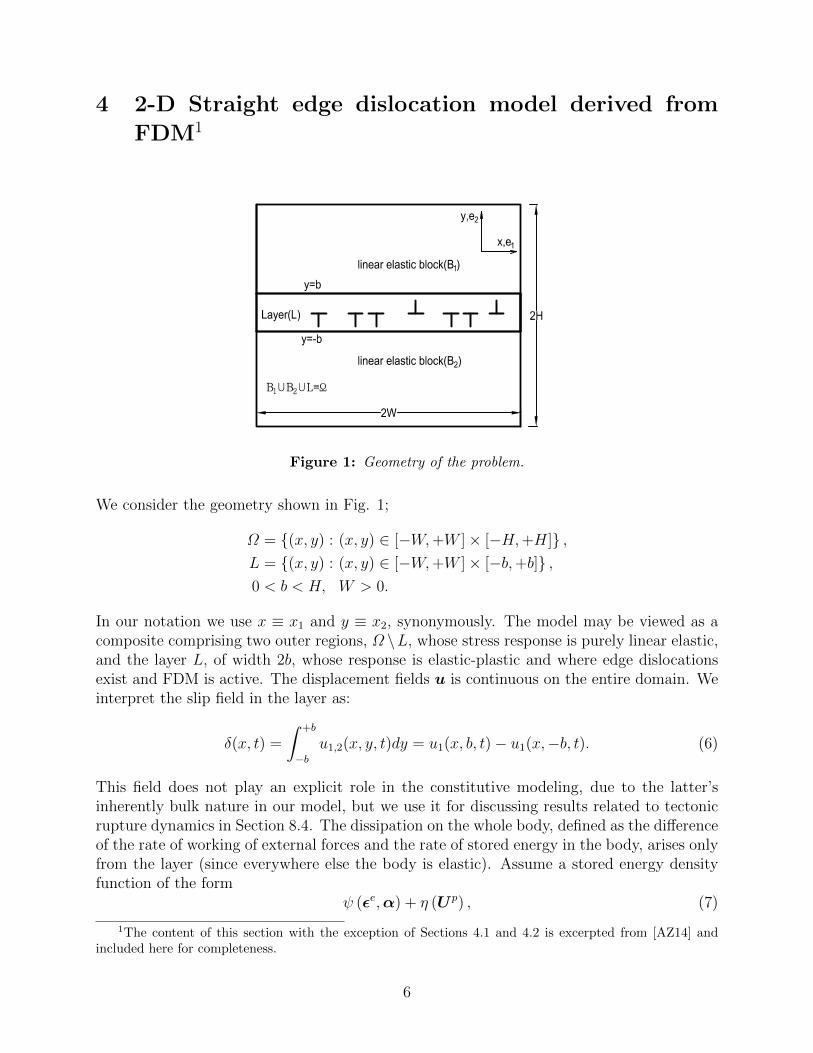
Figure 1: Geometry of the problem.

We consider the geometry shown in Fig. 1;

Ω = (x, y) : (x, y) ∈ [−W,+W ]× [−H,+H] ,L = (x, y) : (x, y) ∈ [−W,+W ]× [−b,+b] ,0 < b < H, W > 0.

In our notation we use x ≡ x1 and y ≡ x2, synonymously. The model may be viewed as acomposite comprising two outer regions, Ω \L, whose stress response is purely linear elastic,and the layer L, of width 2b, whose response is elastic-plastic and where edge dislocationsexist and FDM is active. The displacement fields u is continuous on the entire domain. Weinterpret the slip field in the layer as:

δ(x, t) =

∫ +b

−bu1,2(x, y, t)dy = u1(x, b, t)− u1(x,−b, t). (6)

This field does not play an explicit role in the constitutive modeling, due to the latter’sinherently bulk nature in our model, but we use it for discussing results related to tectonicrupture dynamics in Section 8.4. The dissipation on the whole body, defined as the differenceof the rate of working of external forces and the rate of stored energy in the body, arises onlyfrom the layer (since everywhere else the body is elastic). Assume a stored energy densityfunction of the form

ψ (εe,α) + η (U p) , (7)

1The content of this section with the exception of Sections 4.1 and 4.2 is excerpted from [AZ14] andincluded here for completeness.

6

with stress given by T = ∂ψ/∂εe , where εe is the symmetric part of the elastic distortion U e.The function ψ is assumed to be positive-definite quadratic in εe and the function η is multi-well non-convex, endowing the energy function with barriers to slip and conferring preferredenergetic status to certain plastic strains than others. Together, these two functions enablethe robust modeling of overall total strain distributions in the layer displaying localized,smooth transitions between slipped and unslipped regions (or between the preferred strainstates encoded in η). This crucially requires adding an energetic penalty to the developmentof high values of the dislocation density α, referred to as a core energy. In effect, the linearelastic stress and the core term tend to prevent a sharp discontinuity and the driving forcefrom the non-convex η term promotes the discontinuity, and it is the balance between thesethermodynamic forces that sets the dislocation core width at equilibrium. Interestingly, itcan be shown that while in the presence of just one component of plastic distortion onlythe linear elastic term suffices to give a finite core width (paralleling a fundamental resultdue to Peierls [Pei40]), with more than one component, the core regularization from theα term is essential [AT11, LS08]. It is to be noted that the core energy is a fundamentalphysical ingredient of our model and not simply a mathematical regularization. In general,it is not expected to have the simple ‘isotropic’ form assumed here and, in fact, its character-ization furnishes our model with a direct route of making contact with (sub)atomic physics[MPBO98, IRG15].

The dissipation in the model can be written as

D =

∫L

(T − ∂η

∂U p

): U pdv +

∫L

∂ψ

∂α: curl (α× V ) dv

=

∫L

(T − ∂η

∂U p

): (α× V ) dv +

∫L

curl

(∂ψ

∂α

): α× V dv

+

∫∂L

∂ψ

∂α: (α× V )× nda

where n is the outward unit normal field to the body.In the layer assume the ansatz

U p (x, y, t) = Up12 (x, y, t) e1 ⊗ e2 + Up

22 (x, y, t) e2 ⊗ e2

:= φ(x, t)e1 ⊗ e2 + ω(x, t)e2 ⊗ e2

(8)

where the functions φ(x, t), ω(x, t) need to be defined.Then

α (x, y, t) = − curlU p (x, y, t) = −φx (x, t) e1 ⊗ e3 − ωx (x, t) e2 ⊗ e3 (9)

andcurlα (x, y, t) = φxx (x, t) e1 ⊗ e2 + ωxx (x, t) e2 ⊗ e2.

In keeping with the 2-d nature of this analysis and the constraint posed by the layer on thedislocation velocity, we assume

V (x, y, t) = V1 (x, y, t) e1 := v(x, t)e1

7

where v(x, t) needs to be defined.Note that with these assumptions, the boundary term in the dissipation vanishes for the

horizontal portions of the layer boundary. We also assume

∂ψ

∂α= εα,

where ε is a parameter with physical dimensions of stress× length2 that introduces a lengthscale and essentially sets the width of the dislocation core, at equilibrium. For specificsimplicity in this problem, we impose α = 0 on vertical portions of the layer boundary byimposing φx (±W, t) = ωx (±W, t) = 0.

With the above ansatz, the conservation law α = − curl (α× V ) reduces to

φt (x, t) = −φxv (x, t) or α1t = − (α1v)xωt (x, t) = −ωxv (x, t) or α2t = − (α2v)x ,

(10)

where α1 := −φx = α13 and α2 := −ωx = α23. Equation 10 defines the evolution equationsfor the plastic distortion components φ, ω once v is defined as a function of (x, t).

We now consider the dissipation

D =

∫L

V1

e1j3

(T − A+ ε(curlα)T

)jrαr3

dv Ajr :=

(∂η

∂U p

)jr

=

∫L

v (x, t)

[T12 (x, y, t)− A12 (x, t) + εφxx (x, t)] (−φx (x, t))

+ [T22 (x, y, t)− A22 (x, t) + εωxx (x, t)] (−ωx (x, t))

dv.

We make the choice

v(x, t) :=−1

Bm lm−1 |α|m (x, t)

φx(x, t)

[τ(x, t)− τ b(x, t) + εφxx(x, t)

]+ωx(x, t)

[σ(x, t)− σb(x, t) + εωxx(x, t)

]m = 0, 1 or 2

τ(x, t) :=1

2b

∫ b

−bT12(x, y, t)dy; τ b := A12

σ(x, t) :=1

2b

∫ b

−bT22(x, y, t)dy; σb := A22

(11)

(i.e. kinetics in the direction of driving force [Ric71], in the context of crystal plasticitytheory), where B = Bm l

m−1|α|m is a non-negative drag coefficient that characterizes theenergy dissipation by specifying how the dislocation velocity responds to the applied drivingforce locally and l is an internal length scale, e.g. Burgers vector magnitude of crystals. Forsimplicity, we assume the drag to be a scalar but in general its inverse, the mobility, couldbe a positive-semidefinite tensor. In general, it is in B that one would like to model theeffect of layer structural inhomogeneities impeding dislocations as well as the effect of othermicroscopic mechanisms of energy dissipation during dislocation motion.

The parameter Bm is expected, in general, to be a function of m; however, for all valuesof m, Bm has physical dimensions of stress× time× length−1, and introduces another lengthscale related to kinetic effects.

8

Then the dissipation becomes

D =

∫L

1

Bm lm−1|α|m(x, t)

φx(x, t)

[τ(x, t)− τ b(x, t) + εφxx(x, t)

]+ωx(x, t)

[σ(x, t)− σb(x, t) + εωxx(x, t)

]2

dxdy

+ R,

where

R =

∫ x=+W

x=−W−v(x, t)

φx(x, t)

∫ b

−b[T12(x, y, t)− τ(x, t)] dy

+ωx(x, t)

∫ b

−b[T22(x, y, t)− σ(x, t)] dy

dx.

Recalling the definitions of the layer-averaged stresses τ, σ in (11), we observe that

R = 0 and D ≥ 0.

To summarize, within the class of kinetic relations for dislocation velocity in terms of drivingforce, positive dissipation along with the (global) conservation of Burgers vector contentgoverns the nonlinear and nonlocal slip dynamics of the model. Essentially, slip gradientsinduce stress and elastic energy and the evolution of the dislocation is a means for the mediato relieve this energy, subject to conservation of mass, momentum, energy, and Burgersvector.

To further simplify matters, we make the assumption that ω ≡ 0, i.e. no normal plasticstrain in the composite layer. Suppressing the argument (x, t), the governing equation forthe plastic shear strain now becomes

φt =|φx|2

Bm lm−1|α|m(τ − τ b + εφxx).

The parameter m can be chosen to probe different types of behaviour. Especially, m = 0corresponds to the simplest possible (linear) kinetic assumption. Recall that

τ(x, t) :=1

2b

∫ b

−bT12(x, y, t)dy and τ b(x, t) =

∂η

∂φ.

For the stored energy, we assume the form

1

2εe : Cεe + η(U p) +

1

2ε|α|2, (12)

where εe is the elastic strain tensor. The non-convex energy density function is chosen to bea multiple well potential, with the plastic shear strain values at its minima representing thepreferred plastic strain levels. A typical candidate that we utilize in this paper is

η =µφ2

π2

(1− cos(2π

φ

φ)

). (13)

The displacement field in the model satisfies

ρui = Tij,j in Ω

9

where, for an isotropic material,

Tij = λεekkδij + 2µεeij,

λ, µ being the Lame parameters and

Eij :=1

2(ui,j + uj,i)

εeij = Eij in the elastic blocks, i.e. Ω \ L

εe12 = εe21 = E12 −φ

2; all other εeij = Eij in the fault layer L,

where i, j take the values 1, 2. The governing equations of the system are thusρ∂2ui∂t2

=∂Tij∂xj

in Ω

∂φ

∂t=

1

Bm lm−1

∣∣∣∣ ∂φ∂x1

∣∣∣∣2−m(τ − τ b + ε∂2φ

∂x12

)in L.

(14)

We make the choice l = b (fault zone width in rupture dynamics; in crystals, a measureof the interatomic spacing). Then dimensional analysis suggests introducing the followingdimensionless variables:

x =x

b, t =

Vst

b, u =

u

b, T =

T

µ, τ b =

τ b

µ, ε =

ε

µb2, Bm =

Vsµ/Bm

(15)

where µ is the shear modulus and Vs =√µ/ρ is the elastic shear wave speed of the material.

The non-dimensional drag number Bm represents the ratio of the elastic wave speed of thematerial to an intrinsic velocity scale of the layer material. The non-dimensionalized versionof Eqs. (14) reads as:

∂2ui

∂t2=∂Tij∂xj

in Ω

∂φ

∂t=

1

Bm

∣∣∣∣ ∂φ∂x1

∣∣∣∣2−m(τ − τ b + ε∂2φ

∂x12

)in L.

(16)

The system (16) admits initial conditions on the displacement and velocity fields ui, ˙uiand the plastic strain φ. As mentioned before, we apply the Neumann condition φx = 0on the left and right boundaries of the layer L and for (161) we utilize standard prescribedtraction and/or displacement boundary conditions.

4.1 Bm 1: Quasi-static, rate-dependent response

We consider a generic, appropriately nondimensionalized, loading parameter (either appliedtraction or displacement b.c.s) that evolves as

dτa

dt= Γ, (17)

10

where Γ 1 is a dimensionless loading rate, assumed to be tunable to be as small as required.The restriction to monotonic loading is not essential, but will suffice for our purposes in thispaper. We now introduce a slow time scale

s =t

Bm

(18)

and pose the governing system (16) in this slow time scale:

1

B2m

∂2ui∂s2

=∂Tij∂xj

∂φ

∂s=

∣∣∣∣ ∂φ∂x1

∣∣∣∣2−m(τ − τ b + ε∂2φ

∂x12

)dτa

ds= ΓBm.

We note that Bm 1, and require Γ ≤ B−1m . Moreover, we assume evolutions restricted to

∂2ui∂s2

= O(1) (in the limit Bm →∞) to obtain the quasi-static system

0 =∂Tij∂xj

∂φ

∂s=

∣∣∣∣ ∂φ∂x1

∣∣∣∣2−m(τ − τ b + ε∂2φ

∂x12

)dτa

ds= O(1).

(19)

For m = 2, (192) has the form of a nonlocal Ginzburg-Landau (NGL) equation and form = 1, that of a nonlocal level set (NLS) equation. To our knowledge, the case m = 0corresponding to the simplest and most natural constitutive assumption for the dislocationvelocity (i.e. a linear kinetic ‘law’) seems not to have been previously considered. We name itthe nonlocal generalized Burgers (NGB) equation based on the following reasoning: when thecoefficient of the first derivative term is a constant, the equation is indeed, up to a rescalingin time, the inviscid Burgers equation in Hamilton-Jacobi form. Of course, the coefficientis not a constant and contains a ‘viscous regularization’ that comes not as a uniform, linearparabolic term as in Burgers’ original equation, but in a degenerate quasilinear parabolicform (see [AT11] for some implications), along with nonlocal and nonmonotone contributions.Regardless, for the lack of a better choice, the necessity of having a name to refer the equationby, and a desire to note the wonderful confluence of J. M. Burgers’ contributions in fluiddynamics and crystal dislocations within our model, we christen the equation by the namewe have adopted. Indeed, a distinguishing feature of Burgers equation is the modeling ofshape-change of a wave profile with time-evolution and we find that it is this property of ourNGB equation that allows it to predict a Peierls stress-like threshold for dislocation motion.

The quasi-static system (19) evolves on a time scale set by the drag coefficient under veryslow or static loadings. Physically, we may expect this model to be of relevance to slippingin geomaterials and special situations in rupture dynamics [RCF04, CAS99], and polymericcomposites under very slow loading rates.

11

4.2 Bm < 1: Quasi-static, rate-independent response

This case is relevant to dislocation motion in crystalline materials under slow loadings. Fordislocation motion well below the speed of sound, a typical value of the dislocation dragcoefficient used in discrete dislocation methodology is 10−4Pa · s for Aluminum [KCC+92].The ratio of the product of the magnitudes of the shear stress acting on a discrete dislocationand its Burgers vector to this parameter, say BDD, is assumed to be the constitutive equationfor the magnitude of the discrete dislocation’s velocity. In order to estimate the magnitudeof Bm for our model corresponding to crystalline materials, we consider (14)2 for m = 1 and

observe that the coefficient of∣∣∣ ∂φ∂x1 ∣∣∣ corresponds to the velocity of a slip front (whose derivative

represents a dislocation herein) since, for a φ profile monotone increasing/decreasing in x,this is just the first-order wave equation (cf. [VBAF06]). In particular, if τd is a constantapplied stress value and b the Burgers vector magnitude,

τdB1

=τd b

BDD

,

which is just the statement of equality of speeds of dislocations in discrete dislocation method-ology and our model, for m = 1. Using the abovementioned value of BDD from [KCC+92],we obtain

B1 = 0.0297 (20)

after non-dimensionalization according to (15). As mentioned earlier, Bm, for all valuesof m, has the same physical dimension as B1 and in the following we assume them ashaving a common value except in one instance which we explicitly mention in Section 8.1.The non-dimensional, quasi-static systems analyzed herein (19, 22) do not require explicitconsideration of the values of Bm.

We consider slow loading of the type (17) with Γ 1, and a slow time scale of the form

s = Γ t.

On this time scale, the governing equations (16) take the form

Γ 2∂2ui∂s2

=∂Tij∂xj

ΓBm∂φ

∂s=

∣∣∣∣ ∂φ∂x1

∣∣∣∣2−m(τ − τ b + ε∂2φ

∂x12

)dτa

ds= 1.

(21)

Noting that Γ 1 and Bm < 1, we obtain the following quasi-static system:

0 =∂Tij∂xj

0 =

∣∣∣∣ ∂φ∂x1

∣∣∣∣2−m(τ − τ b + ε∂2φ

∂x12

)dτa

ds= 1.

(22)

12

On time intervals in which (22) is an accurate approximation of the actual dynamics, theequivalent dynamics viewed on the fast time scale is (16), appended with

dτa

dt≈ 0.

We note an important fact related to the appropriateness of quasi-static systems like (22).Consider Υ and Φ as the ui(·) and ϕ(·) fields on the body (viewed as functions of spatialcoordinates alone) that satisfy the first two equations of (22) subject to boundary conditionsfor a particular value of the load τa (the load here can be thought of as a function on theboundary of the body). This can be stated abstractly as the fact that (Υ, Φ, τa) satisfy thefunctional equations

F (Υ, Φ, τa) = 0.

Suppose now that the solution set of (Υ, Φ, τa)-triples of the functional equation F =0 (the equilibrium set) admits connected one-dimensional paths. Let one such path be(Υ (s), Φ(s), τa(s)), where the function τa satisfies (223). Then one can compute first andsecond partial derivatives with respect to s of the fields ui and ϕ corresponding to this‘equilibrium’ path and, in general, these are not expected to vanish, even though the pathbelongs to the equilibrium set. However, due to the availability of the small parameters in(21), such a time-dependent ‘solution’ may be considered an appropriate approximate solu-tion of the system (21). It is a remarkable fact that the full dynamics often does follow theseequilibrium paths to a very good approximation. However, situations arise when states arereached along such paths where dτa

dscan no longer be linked uniquely to (dΥ

ds, dΦds

). In thesecircumstances, the quasi-static system (22) provides no guidance on the actual evolutionand only the full dynamics can decide whether jumps, on the slow time scale, between twoequilibrium paths take place (if the τa corresponds to multiple states on the equilibrium setat the instant of the jump) or a single equilibrium path can be followed, or the equilibriumset is abandoned forever by the actual dynamics. At such instants, the time-derivatives in(21) become unbounded and (22) is no longer an appropriate representation of the dynamics(21). The time derivatives in the fast system (16) remain well-behaved, and it is this systemthat needs to be considered for accurate information on the actual dynamics.

When (22) is valid, (dΥds, dΦds

) associated with any state on an equilibrium path is relatedto dτa

dsthrough a linear operator that solely depends on the said state. This represents rate-

independent response where the model has no internal time-scale and the evolution of fieldsdepend on the rate of loading through a homogeneous function of degree 1.

5 Numerical Schemes

We gather the dimensionless governing equations in one place for convenience and thenprovide the numerical schemes for solving the equations:

∂2ui∂t2

=∂Tij∂xj

in Ω

∂φ

∂t=

1

Bm

∣∣∣∣ ∂φ∂x1

∣∣∣∣2−m(τ − τ b + ε∂2φ

∂x12

)in L

(23)

13

whereTij = Cijkl (uk,l − Up

kl)

Cijkl = λδijδkl + µ (δikδjl + δilδjk)

τ b =2µφ

πsin

(2πφ

φ

).

Material properties are controlled by the Lame constants λ, µ and the dimensionless dragcoefficient Bm together with the core energy ε ≈ µb2. In general, the Finite Element Method(FE) is used to solve the equation for balance of linear momentum in a staggered schemethat utilizes the plastic distortion U p as a given quantity obtained by evolving U p (or φ) inthe remaining part of the scheme. The general computing flow is shown in Fig. 2.

Given material properties, initial conditions(φ0 and u0), boundary conditions, total timeTT , loading history, initial time t = 0

Given uk and φk, calculate φk+1 with upwind-ing finite difference method. Solve div T = ρu

for uk+1 with standard Galerkin and cen-teral difference method based on φk and uk

k = k + 1, t = t + 4t. repeat until t ≥ TT

(a) dynamic equations

Given material properties, initial condi-tions (φ0), boundary conditions, total timeSS, loading history, initial time s = 0

Given uk and φk, calculate φk+1 with upwinding finitedifference method. With φk+1 solve div T = 0 for

uk+1 using standard Galerkin method based on φk+1

k = k + 1, s = s + 4s. repeat until s ≥ SS

(b) quasi-static equations

Figure 2: Flow charts for dynamic (Eqs. (16)) and quasi-static (Eqs. (19)) models: φ and u areunkonwn plastic strain and displacement fields. T is Cauchy stress.

An FE mesh with an embedded 1-d finite difference grid is used. We use linear quadri-lateral elements, with 5× 5 Gauss quadrature points. Two types of FE meshes are createdand used:

1. Mesh A: elements are of uniform size over the whole domain.

2. Mesh B : elements are refined in and around the layer area.

Mesh A is used in Sec. 8 as it allows capturing stress wave propagation accurately over thewhole body. Mesh B is used primarily to study the Peierls’ stress problem, e.g., in Sec. 7.1.2and 7.1.5. This is because we need a highly refined mesh in the layer to make statementsindependent of mesh size. We utilize regular quadrilateral elements of uniform size withinthe layer. Outside the layer, the size of the elements increases gradually as they get furtherfrom the layer. The layer is discretized up to 40 elements per Burgers vector, as required,while keeping the overall number of elements less than 150× 103 (Fig. 3).

The 1-d, finite difference grid is embedded in the layer, coincident with the line y = 0.Recall that the layer L is always uniformly meshed (for both meshes A and B). Supposethat the layer is meshed into M rows and N columns, where N is the total number of 1-dgrid points and M is always an odd number so that the middle row of elements always havecentres on y = 0. Each column of FE elements in the layer correspond to exactly one grid

14

point. Let xk be the x coordinate of the kth 1-d grid point, which is at the center of the kthelement in the (M + 1)/2 row of layer elements. The value of U p at each Gauss point withincolumn k is then set to be φ(xk)e1 ⊗ e2, where φ(xk) is the value of φ evaluated at the kth

grid point. Recall that the layer stress τ(xk) is defined as 12b

∫ b−b T12(x, y, t) dy. Let T12(I, k)

denote the stress component T12 at the I th Gauss point whose x coordinate is xk, and let Nk

be the total number of such Gauss points. Then τ(xk) is calculated as

τ(xk) =1

Nk

(Nk∑I=1

T12(I, k)

).

Figure 3: An example of FE mesh used in section 7.1. Elements are refined in and around thelayer.

5.1 Algorithm for evolution problems

The numerical scheme developed in [DAZM13] is adopted and improved to solve (23)2, the φevolution2. The basic idea is to infer the direction of wave propagation from the linearizationof (23)2 and use this direction in the actual nonlinear equation. Let 4t be the time stepand 4h the spatial grid size of the finite difference grid. Due to the necessity of very smallelement sizes to demonstrate convergence, an explicit treatment of the diffusion term in (23)2

becomes prohibitive because of a 4t = O(4h2) scaling. This is circumvented by treatingthe φxx term implicitly, resulting in a linearly implicit scheme as follows. We first linearize

2We thank Dr. Amit Das for his help regarding certain aspects of the implementation described in thisSection.

15

(23)2 and discretize:

δφkt (xh) = −(2−m)

(−sgn

(φkx (xh)

)Bm

)∣∣φkx(xh)∣∣1−m [τ k (xh) + εφk+1xx (xh)−

(τ b (xh)

)k]δφkx (xh)

+

∣∣φkx (xh)∣∣2−m

Bm

[εδφkxx (xh)

]+

∣∣φkx (xh)∣∣2−m

Bm

[τ b′(xh) δφ

k(xh)],

(24)where a quantity such as φkx(xh) implies the value of φx(x) evaluated at hth grid point at kth

time step. The first term in (24) provides an advection equation with wave speed

ck(xh) = (2−m)

(−sgn

(φkx (xh)

)Bm

)∣∣φkx(xh)∣∣1−m [τ k (xh) + εφk+1xx (xh)−

(τ b (xh)

)k].

φkx(xh) and φkxx(xh) are obtained from central finite differences:

φkx(xh) =φk(xh+1)− φk(xh−1)

24h

φkxx(xh) =φk(xh+1)− 2φk(xh) + φk(xh−1)

4h2.

(25)

Based on the sign of ck, φkx is then computed by the following upwinding scheme:

φkx =

φk(xh+1)−φk(xh)

4h if ck(xh) < 0φk(xh)−φk(xh−1)

4h if ck(xh) > 0φk(xh+1)−φk(xh−1)

24h if ck(xh) = 0.

(26)

The time step is governed by a combination of a CFL condition and a criterion for stabilityfor an explicit scheme for a linear ordinary differential equation:

4tk = min

(4hck(xh)

,Bm

|φkx(xh)|2−m(−(τ b′(xh))k

). (27)

Note that if φxx was evaluated at k, then the step size would also be bounded by 4h2Bm

ε|φkx(xh)| ,

leading to a quadratic decrease in 4tk with element size. Treating φxx implicitly eliminatesthis constraint resulting in significant savings in computation time. φk+1

h is updated accordingto

φk+1(xh)− φk(xh)4tk

=|φkx(xh)|2−m

Bm

[τ k + εφk+1

xx − (τ b(xh))k]

⇒φk+1(xh)− ε4tk|φkx(xh)|2−m

Bm

φk+1xx (xh) = φk(xh) +4tk |φ

kx(xh)|2−m

Bm

[τ k − (τ b(xh))

k].

(28)

16

The right hand side of the equation is known at current time k. But noting that φk+1xx (xh) is

again computed from φk+1 at xh+1, xh and xh−1, a system of linear equations of size N hasto be solved to get φk+1. The computational expense of the linear solve is small comparedto the savings obtained by relaxing 4tk corresponding to the explicit treatment of diffusion.

5.2 Algorithm for equilibria

In this section we record the derivation of a Quasi-Newton scheme for system (22), specificallythe φ equation. In Sec. 6, we use this method to determine equilibrium states under zero orfinite loads.

In the following, when we refer to φI we mean the discrete nodal list of values of theapproximation to the function φ on a finite difference grid, corresponding to the I th iteratein the Quasi-Newton scheme. Consider the case m = 0 (NGB) first. The residual for theφ-equation is denoted by F and defined as

∣∣φiJx∣∣2 [τ iJ + εφiJxx −∂η

∂φ

(φiJ)]

=: F i(φJ). (29)

Here, τ iJ is a function of φJ only through φiJ . The notation (·)iJ ··· denotes the value of thediscrete approximation to the function (·)··· corresponding to the J th iterate for φ at the ith

node. The second spatial derivative appearing in (29) is defined as in (25). For the firstspatial derivative, the following scheme is used. Define

ciJ := −2sgn(φiJx)∣∣φiJx∣∣ [τ iJ + εφiJxx −

∂η

∂φ

(φiJ)], (30)

where both φiJx and φiJxx are evaluated from φJ according to (25). With the value of thearray cJ in hand, φiJx is redefined as

φiJx =

φi+1J − φiJ4h

, if ciJ < 0

φiJ − φi−1J

4h, if ciJ > 0

φi+1J − φi−1

J

24h, if ciJ = 0.

(31)

This array of values of φJx is then used in defining the residual (29).The Newton-Raphson scheme obtained from the residual (29) is

−F i(φJ) = −ciJδφix +∣∣φiJx∣∣2 [µδφi + εδφixx −

∂2η

∂φ2

(φiJ)δφi]

φiJ+1 = φiJ + δφi,

(32)

17

where the element δφix of the array of corrections δφ is defined as

δφix =

δφi+1 − δφi

4h, if ciJ < 0

δφi − δφi−1

4h, if ciJ > 0

δφi+1 − δφi−1

24h, if ciJ = 0.

(33)

This Newton-Raphson scheme leads to an asymmetric tridiagonal Jacobian matrix, which isalso singular because the leading term φJx vanishes in dislocation free regions. To deal withthat, we observe the residual also has a multiplier of |φix| and cancel it from both sides of theequation. This results in a Quasi-Newton method where the Jacobian matrix is modified.Of course, the residual is kept exactly in the form (29) without modification. Quasi-Newtoniterations are continued until the l∞ norm of the residual, |F |∞, vanishes (up to a smalltolerance).

For the NGL (m = 2) equation we use the exact Jacobian for the Newton-Raphsonmethod given by

−F i(φJ) = µδφi + εδφixx −∂2η

∂φ2

(φiJ)δφi. (34)

For the NLS equation, we use a Quasi-Newton method based on the Jacobian matrix(34).

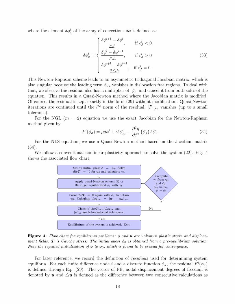
We follow a conventional nonlinear plasticity approach to solve the system (22). Fig. 4shows the associated flow chart.

Set an initial guess φ = φ0. SolvedivT = 0 for u0 and calculate τ0.

Apply quasi-Newton scheme 32 or34 to get equilibrated φ1 with τ0.

Solve divT = 0 again with φ1 to obtainu1. Calculate |4u|∞ = |u1 − u0|∞.

Check if |divT |∞, |4u|∞ and|F |∞ are below selected tolerances.

Computeτ0 from u1

and φ1.u0 := u1,φ := φ0

Equilibrium of the system is achieved. Exit.

No

Yes

Figure 4: Flow chart for equilibrium problems: φ and u are unkonwn plastic strain and displace-ment fields. T is Cauchy stress. The initial guess φ0 is obtained from a pre-equilibrium solution.Note the repeated initialization of φ to φ0, which is found to be crucial for convergence.

For later reference, we record the definition of residuals used for determining systemequilibria. For each finite difference node i and a discrete function φJ , the residual F i(φJ)is defined through Eq. (29). The vector of FE, nodal displacement degrees of freedom isdenoted by u and 4u is defined as the difference between two consecutive calculations as

18

defined in Fig. 4. Both vectors F and 4u are measured by their l∞ norm, i.e., suppose N isthe total number of nodes on the FE mesh (not including nodes on which Dirichlet boundaryconditions are specified) and M is the total number of finite difference grid points, then

|4u|∞ := max1≤i≤2N

|ui|, |F |∞ := max1≤i≤M

|F i| (35)

6 Equilibrium Aspects

We solve some key problems of classical dislocation theory [Nab87, HL82] in this Section,approached as equilibrium states of our dynamical model (16). While the classical theory in-volves singular dislocations with infinite-energy elastic fields (even on finite bodies), our solu-tions have finite energies and nonsingular cores. It is worth emphasizing that our equilibriumcore distributions of dislocation density for a single dislocation are not a model assumptionas in [Ach01, PLSG14, CAWB06]. These fields in our case, along with their correspondingnon-singular stress distributions, correspond to equilibrium states of a dynamic theory whereboth the dislocation (core) distribution and the stress evolve to decrease the free energy ofa body; the solutions in the aforementioned works, in particular the core distributions, haveno such thermodynamic status. The larger implication of this feature is that FDM can serveas an idealized model for studying complex questions related to equilibrium and dynamicevolution (at realistic time-scales) of core structures of single and interacting dislocationsunder loads, utilizing input from finer length-scale models like Density Functional Theory[IRG15] and Molecular statics [Vit68, SW03, MPBO98] in defining its energetic constitutiveingredients (7), (12). Our model for m = 2 (NGL), up to the definition of the layer stressτ and the use of the core energy, is essentially identical to that of the phase field model ofdislocations [WL10, Den04].

6.1 Equilibria of single edge dislocations

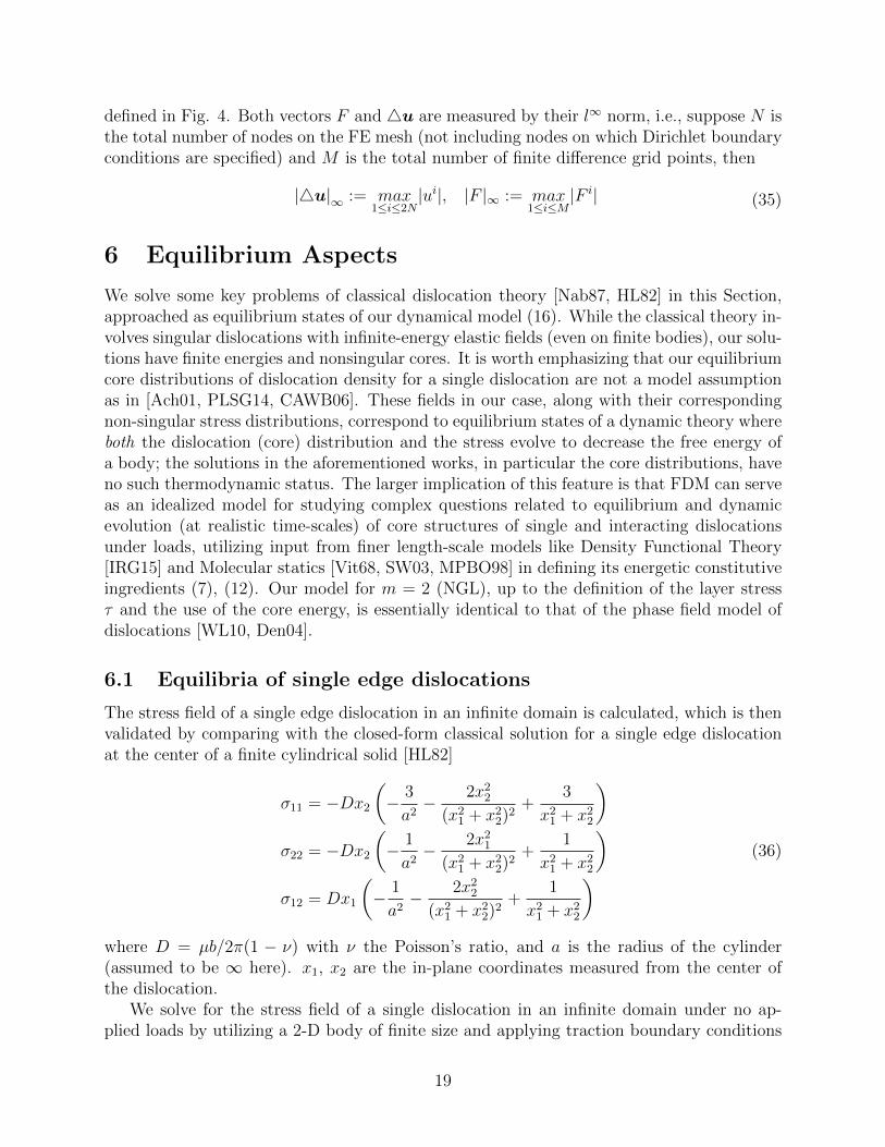
The stress field of a single edge dislocation in an infinite domain is calculated, which is thenvalidated by comparing with the closed-form classical solution for a single edge dislocationat the center of a finite cylindrical solid [HL82]

σ11 = −Dx2

(− 3

a2− 2x2

2

(x21 + x2

2)2+

3

x21 + x2

2

)σ22 = −Dx2

(− 1

a2− 2x2

1

(x21 + x2

2)2+

1

x21 + x2

2

)σ12 = Dx1

(− 1

a2− 2x2

2

(x21 + x2

2)2+

1

x21 + x2

2

) (36)

where D = µb/2π(1 − ν) with ν the Poisson’s ratio, and a is the radius of the cylinder(assumed to be ∞ here). x1, x2 are the in-plane coordinates measured from the center ofthe dislocation.

We solve for the stress field of a single dislocation in an infinite domain under no ap-plied loads by utilizing a 2-D body of finite size and applying traction boundary conditions

19

according to the analytical stress field. Specifically, we compute the analytical stress σ∗ ofboundary points according to Eqs. (36) and then apply a boundary traction t = σ∗n, wheren is the outward unit normal to the boundary. The rigid deformation of the body is removedby fixing u1 and u2 at the corner (−W,−H) as well as fixing u2 at (W,−H).

We are interested in obtaining special equilibria of the system (16) corresponding to thefield of a single dislocation. Because of the degenerate and nonlinear nature of the equilibriumequations for m = 0, 1, approaching the question by directly trying to approximate equilibriais a formidable task. Instead, evolution to equilibrium could be a desirable route. However,the time scale of evolution of (16) is extremely restrictive and since equilibrium states arethe only items of concern here, the question could as well be approached by evolving thequasi-static dynamics (19) from suitably close initial conditions. There is a complication inthat the system (19) belongs to a class in which simpler versions [CP89, DAZM13] exhibitextremely sluggish dynamics out of states which, nevertheless, are known not to be equilibria.Thus, we adopt the following approach:

1. We consider all m = 0 (NGB), m = 1 (NLS) and m = 2 (NGL) models. The initialcondition on φ is a hyperbolic tangent function whose first spatial derivative givesthe initial distribution of the dislocation density according to (9) representing a singledislocation:

φ(x, t = 0) =1

2

(φ tanh(a x) + φ

), (37)

where we choose φ = 0.5, and a =√µ/4ε. By the definition of α, the initial Burgers

vector magnitude b0 may be approximated as b0 =∫L

∫d−φx(x, 0) e3 dydx ≈ −2φb =

−b.

2. The dynamics (19) is evolved to get to a state that satisfies approximate equilibriumconditions up to certain numerical tolerances. We conservatively specify a thresholdvalue of |φs|∞ < 5× 10−5, where |φs|∞ represents the l∞ norm of the discrete φ field,i.e. |φs|∞ := max

1≤i≤N|φis|, (N being the total number of finite difference nodes.). This

threshold is conservative because the profile-change of the dislocation field becomesindiscernible to the eye long before |φs|∞ gets to this value.

We refer to these practically static states as dislocation pre-equilibria.

3. We use the NGL, NLS, NGB dislocation pre-equilibrium states as initial guesses tosolve the corresponding nonlinear equilibrium equations of (16). The numerical imple-mentation is described in Section 5. Dimensionless tolerances required by the schemeto determine whether an equilibrium state is achieved are chosen as follows:

|4u|∞ < 2× 10−4, |F |∞ < 5× 10−10. (38)

Recall that |F |∞ measures the residual of the φ equilibrium equation (and therefore ourtolerance requires equilibria to be at least 5 orders of magnitude slower than dislocationpre-equilibria); |4u|∞ measures the residual of the displacement fields between twoconsecutive approximations; |divT |∞ tests mechanical force balance, which is alwaysresolved on the scale of 10−15.

20

We refer to the attained solutions as (unloaded) NGL/NLS/NGB dislocation equilibria.

Furthermore, in what follows, we need the following definitions:

• Equilibria of the NGB dynamics are sought, closest to an NGL dislocation pre-equilibria in the sense of the latter serving as an initial guess for the procedureoutlined above (i.e. list item 3). We refer to such an equilibrium state as anNGL-s-NGB dislocation equilibrium (the ‘s’ stands for ‘start’).

• NGB equilibrium states are sought, as defined above, but now under the actionof a nonzero applied traction on the body. We refer to such a state as a loadedNGB dislocation equilibrium.

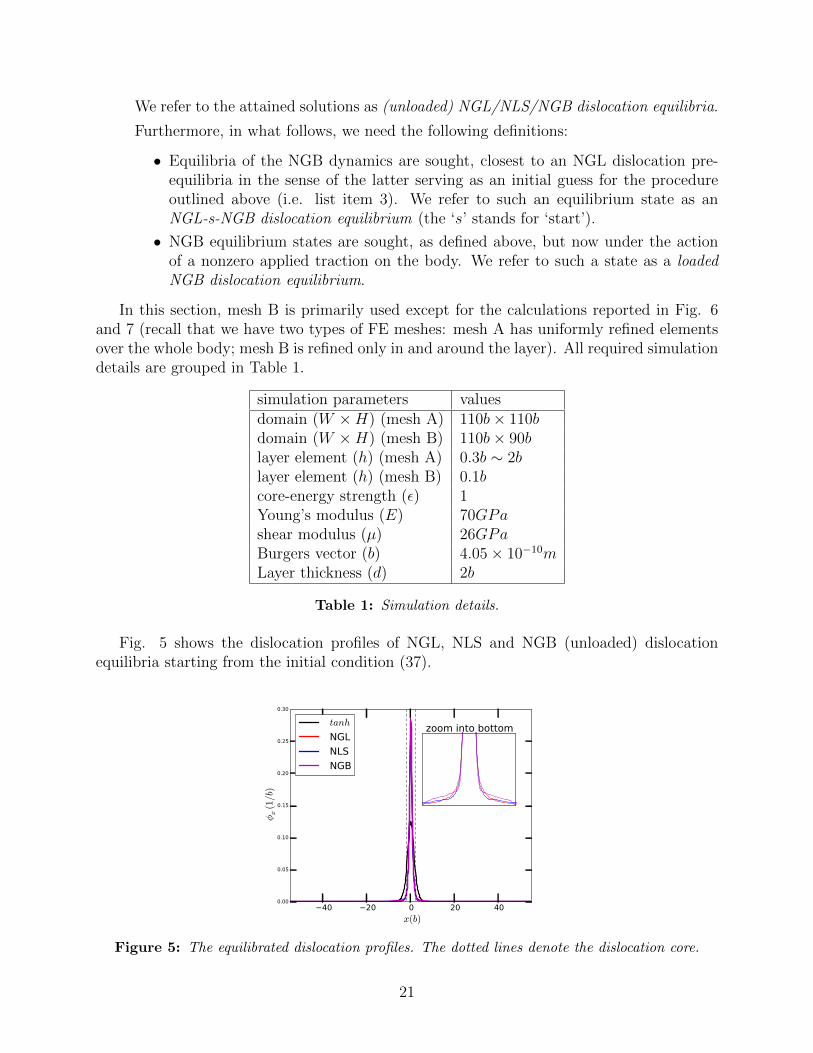
In this section, mesh B is primarily used except for the calculations reported in Fig. 6and 7 (recall that we have two types of FE meshes: mesh A has uniformly refined elementsover the whole body; mesh B is refined only in and around the layer). All required simulationdetails are grouped in Table 1.

simulation parameters valuesdomain (W ×H) (mesh A) 110b× 110bdomain (W ×H) (mesh B) 110b× 90blayer element (h) (mesh A) 0.3b ∼ 2blayer element (h) (mesh B) 0.1bcore-energy strength (ε) 1Young’s modulus (E) 70GPashear modulus (µ) 26GPaBurgers vector (b) 4.05× 10−10mLayer thickness (d) 2b

Table 1: Simulation details.

Fig. 5 shows the dislocation profiles of NGL, NLS and NGB (unloaded) dislocationequilibria starting from the initial condition (37).

40 20 0 20 40

x(b)

0.00

0.05

0.10

0.15

0.20

0.25

0.30

φx(1/b

)

tanh

NGL

NLS

NGB

zoom into bottom

Figure 5: The equilibrated dislocation profiles. The dotted lines denote the dislocation core.

21

The quantity τ is of primary interest in this section as it is analogous to σ12 of Eq.(36) with x2 = 0. Figures 6, 7(a) and 7(b) together demonstrate that the numerical stressfield obtained from our model is quantitatively comparable to that from classical solutions.In particular, Fig. 6 shows that the stress field does not strictly rely on a highly refinedmesh, i.e., a mesh as coarse as h = 2b can still provide a stress result consistent with theclassical solution outside the dislocation core. As shown in Fig. 6, the difference between theequilibrated averaged layer stress τ (blue) and the analytical solution along x axis (cyan) isindiscernible beyond the dislocation core (marked by the two dotted lines).

40 20 0 20 40

x(b)

0.10

0.05

0.00

0.05

0.10

τ(µ

)

τ ∗

h=0.3b

h=1b

h=2b

Figure 6: Comparison of τ with the analytical solution at x = 0. The dotted lines denote thedislocation core. τ∗ is a closed-form T12 on x1 axis from the classic method. h is the finite elementsize in the layer, measured with Burgers vector.

Fig. 7(a) shows the contour of shear stress σ12 on the body. The difference between thenumerical and the closed-form classical solution is quantified by calculating an error measureER defined by

ERij(x, y) =

∣∣σ∗ij(x, y)− σij(x, y)∣∣∣∣σ∗ij(x, y)

∣∣ , (39)

where σ∗ij and σij are the solutions from (36) and numerical computation, respectively. At the

lines x = 0 and x = ±y where the denominator∣∣σ∗ij∣∣ vanishes, ER12 values are not plotted.

The maximum value of σ12 along these ‘blank’ regions given by our model is 5.7 × 10−5µwhich is achieved on the boundaries of the dislocation core. Some other data points along thelines are: 4.6573×10−6µ at (30b, 30b) and 1.4360×10−5µ at (50b, 50b). To sum up, it can beconcluded that the error (ER12) is primarily restricted to the core area; the overall patternsand values are in close agreement. ER12 reaches up to around 40% at the core boundaries dueto the (unphysical) singularity of the analytical solution. Similar comparisons are obtainedfor other stress components for both the NLS and NGB cases. We think of such dislocatedstates in an unloaded body as stressed metastable states.

22

(a) Equilibrated FDM stress field σ12 of the edgedislocation in an infinite media.

(b) ER12: a measure of difference between FDMresults and the analytical results outside the core.

Figure 7: Comparison of numerical stress with analytical solution.

Two important observations on unloaded dislocation equilibria are:

• The (unloaded) NGL dislocation equilibrium is found to be identical to the NGL-s-NGB dislocation equilibrium. The former is also an equilibrium state for the NLSdynamics. These are verifications for our numerical procedures as it is easy to see thatan equilibrium state for the NGL dynamics must be so for both the NLS and NGBdynamics.

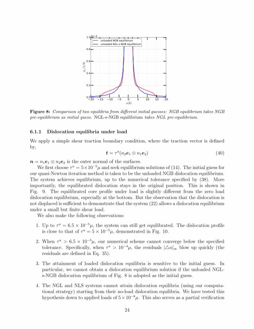
• We find that the shapes of the NGB dislocation equilibrium (obtained from the NGBdislocation pre-equilibria) and the NGL-s-NGB dislocation equilibrium are different.One needs to zoom into the bottom of Figure 5 to appreciate this difference, which isshown in Fig. 8. Apparently, the NGB dislocation equilibrium leads to a profile withcurved steps on both sides of the core while the NGL-s-NGB dislocation equilibriumhas a smooth profile with no steps.

This difference of shape will be further discussed in the following Section as it producescompletely different solutions for loaded problems.

23

20 15 10 5 0 5 10 15 20 x(b)

0.0

0.2

0.4

0.6

0.8

1.0

φx(1/b

)

1e 2

unloaded NGB equilibrium

unloaded NGL-s-NGB equilibrium

Figure 8: Comparison of two equilibria from different initial guesses: NGB equilibrium takes NGBpre-equilibrium as initial guess. NGL-s-NGB equilibrium takes NGL pre-equilibrium.

6.1.1 Dislocation equilibria under load

We apply a simple shear traction boundary condition, where the traction vector is definedby,

t = τa(n2e1 ⊗ n1e2) (40)

n = n1e1 ⊗ n2e2 is the outer normal of the surfaces.We first choose τa = 5×10−5µ and seek equilibrium solutions of (14). The initial guess for

our quasi-Newton iteration method is taken to be the unloaded NGB dislocation equilibrium.The system achieves equilibrium, up to the numerical tolerance specified by (38). Moreimportantly, the equilibrated dislocation stays in the original position. This is shown inFig. 9. The equilibrated core profile under load is slightly different from the zero loaddislocation equilibrium, especially at the bottom. But the observation that the dislocation isnot displaced is sufficient to demonstrate that the system (22) allows a dislocation equilibriumunder a small but finite shear load.

We also make the following observations:

1. Up to τa = 6.5 × 10−5µ, the system can still get equilibrated. The dislocation profileis close to that of τa = 5× 10−5µ, demonstrated in Fig. 10.

2. When τa > 6.5 × 10−5µ, our numerical scheme cannot converge below the specifiedtolerance. Specifically, when τa > 10−4µ, the residuals |4u|∞ blow up quickly (theresiduals are defined in Eq. 35).

3. The attainment of loaded dislocation equilibria is sensitive to the initial guess. Inparticular, we cannot obtain a dislocation equilibrium solution if the unloaded NGL-s-NGB dislocation equilibrium of Fig. 8 is adopted as the initial guess.

4. The NGL and NLS systems cannot attain dislocation equilibria (using our computa-tional strategy) starting from their no-load dislocation equilibria. We have tested thishypothesis down to applied loads of 5×10−8µ. This also serves as a partial verification

24

of our numerical procedures since it can be shown that a no-load single dislocationequilibrium profile in an infinite body for the NLS dynamics has to move as a rigidtraveling wave with uniform speed under arbitrary, non-zero applied loads.

30 20 10 0 10 20 30

x(b)

0.0

0.2

0.4

0.6

0.8

1.0

φx(1/b

)

1e 2

unloaded equilibrium

loaded equilibrium

Figure 9: Equilibrium for load 5×10−5µ, com-pared to unloaded NGB dislocation equilibrium.

30 20 10 0 10 20 30

x(b)

0.0

0.2

0.4

0.6

0.8

1.0

φx(1/b

)

1e 2

τa =5×10−5µ

τa =6.5×10−5µ

Figure 10: Equilibria for loads 5× 10−5µ and6.5× 10−5µ are on top of each other.

In order to better understand the difference between the NGB and NGL models withrespect to attainment of equilibrium under load, we analyze and plot the two constituentparts of their residuals: the energetic driving force term (τ + εφxx − τ b) and the leadingtransport term (φ2

x of NGB, 1 of NGL). The energetic driving force terms are shown inFig. 11(a) and 11(b). Specifically, the NGB case corresponds to a loaded equilibriumstate of τa = 5 × 10−5µ. Since the NGL dynamics cannot sustain a loaded equilibrium,we consider one particular state during its quasi-static evolution according to (19) underthe same constant applied load. An immediate observation is as follows. Even though theenergetic driving force for the NGB model is much greater in magnitude outside the core thanits NGL counterpart, its ‘transport multiplier,’ φ2

x, essentially vanishes beyond [−3.5b, 3.5b];within [−3.5b, 3.5b], the NGB energetic driving force happens to be extremely close to zero(as shown in the inset of Fig. 11(b)). To the contrary, NGL has an all-positive energeticdriving force after load is applied, with especially large values in the core area, and NGLdoes not have any leading transport term to counterbalance this effect and stop dislocationmotion.

25

60 40 20 0 20 40 600.000.010.020.030.040.050.060.070.080.09

φ 2x

60 40 20 0 20 40 60

x(b)

0.015

0.010

0.005

0.000

0.005

0.010

0.015

τ+εφxx−τb

(a) NGB

15 10 5 0 5 10 15

x(b)

0.0

0.2

0.4

0.6

0.8

1.0

τ+εφ

xx−τb

1e 4

3 2 1 0 1 2 31.0

0.5

0.0

0.5

1.01e 4 NGB

(b) NGL

Figure 11: Comparison of equilibrium and motion of NGB and NGL single dislocations underload 5× 10−5µ.

Thus, the attainment of NGB equilibria under load is not simply a matter of getting theenergetics of a model right but delicately dependent on the form of the dynamics, which inthis case follows from the conservation of Burgers vector on dislocation density evolution.Said another way, equilibria in dynamic models need not necessarily be a consequence ofenergetics alone.

6.2 The failure of Linear Elasticity in sustaining a compact core

Figures 12 shows the inadequacy of the use of just linear elasticity, i.e. without any noncon-vexity in the stored energy function, in producing an equilibrium dislocation with a compactcore (we use the word ‘compact’ here to simply mean ‘spatially localized’). Dislocation (pre-)equilibria of (19) are sought under no applied load, now with η ≡ 0 and ε = 0 in (12), so thatthe stored energy function simply contains the linear elastic term. All three dynamics startfrom the same tanh function (37). Although mechanical equilibrium (i.e. force balance) issatisfied at each time step of the dynamics (19), the dislocation density field is unable tosustain a compact core and spreads out thinly over the domain (the Burgers vector vectorcontent has to be conserved with the Neumann boundary conditions (on φx) in force).

26

40 20 0 20 40

x(b)

0.00

0.05

0.10

0.15

0.20 φx(1/b

)

s=0

s=1935

(a) m = 2

40 20 0 20 40

x(b)

0.00

0.05

0.10

0.15

0.20

φx(1/b

)

s=0

s=1935

(b) m = 1

40 20 0 20 40

x(b)

0.00

0.05

0.10

0.15

0.20

φx(1/b

)

s=0

s=1935

(c) m = 0

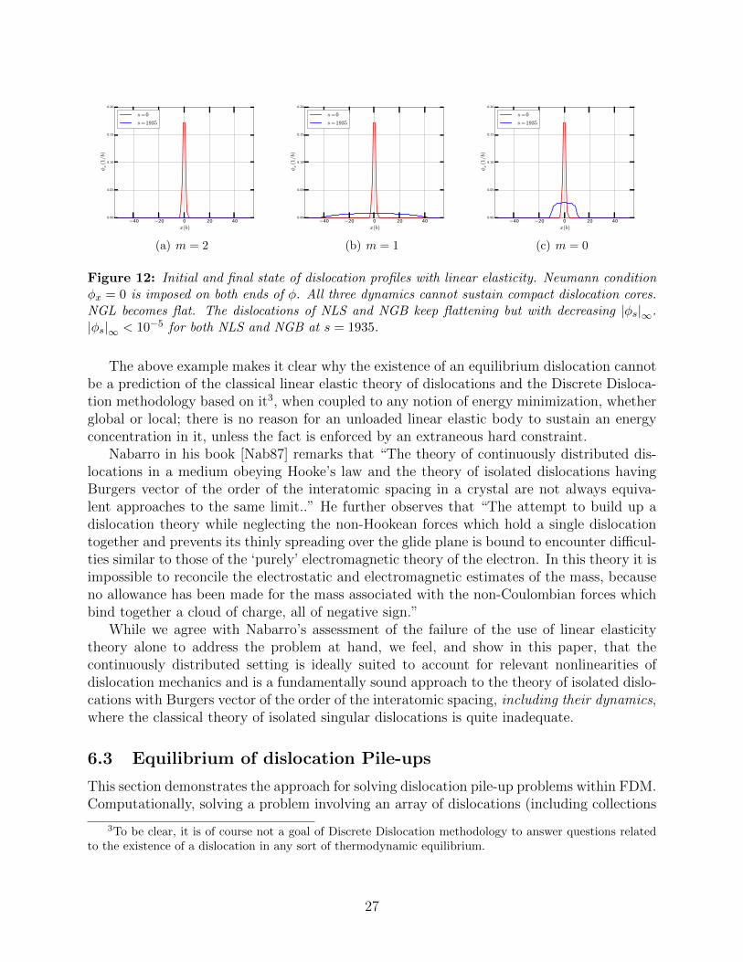
Figure 12: Initial and final state of dislocation profiles with linear elasticity. Neumann conditionφx = 0 is imposed on both ends of φ. All three dynamics cannot sustain compact dislocation cores.NGL becomes flat. The dislocations of NLS and NGB keep flattening but with decreasing |φs|∞.|φs|∞ < 10−5 for both NLS and NGB at s = 1935.

The above example makes it clear why the existence of an equilibrium dislocation cannotbe a prediction of the classical linear elastic theory of dislocations and the Discrete Disloca-tion methodology based on it3, when coupled to any notion of energy minimization, whetherglobal or local; there is no reason for an unloaded linear elastic body to sustain an energyconcentration in it, unless the fact is enforced by an extraneous hard constraint.

Nabarro in his book [Nab87] remarks that “The theory of continuously distributed dis-locations in a medium obeying Hooke’s law and the theory of isolated dislocations havingBurgers vector of the order of the interatomic spacing in a crystal are not always equiva-lent approaches to the same limit..” He further observes that “The attempt to build up adislocation theory while neglecting the non-Hookean forces which hold a single dislocationtogether and prevents its thinly spreading over the glide plane is bound to encounter difficul-ties similar to those of the ‘purely’ electromagnetic theory of the electron. In this theory it isimpossible to reconcile the electrostatic and electromagnetic estimates of the mass, becauseno allowance has been made for the mass associated with the non-Coulombian forces whichbind together a cloud of charge, all of negative sign.”

While we agree with Nabarro’s assessment of the failure of the use of linear elasticitytheory alone to address the problem at hand, we feel, and show in this paper, that thecontinuously distributed setting is ideally suited to account for relevant nonlinearities ofdislocation mechanics and is a fundamentally sound approach to the theory of isolated dislo-cations with Burgers vector of the order of the interatomic spacing, including their dynamics,where the classical theory of isolated singular dislocations is quite inadequate.

6.3 Equilibrium of dislocation Pile-ups

This section demonstrates the approach for solving dislocation pile-up problems within FDM.Computationally, solving a problem involving an array of dislocations (including collections

3To be clear, it is of course not a goal of Discrete Dislocation methodology to answer questions relatedto the existence of a dislocation in any sort of thermodynamic equilibrium.

27

with positive and negative dislocations) is essentially the same as solving a single dislocationproblem, except for a change of the initial condition on the field φ.

A key classical problem of the theory of dislocations is the following. A set of dislocationsof identical sign lie on a slip plane. The set of dislocations pile up against obstacles, usuallygrain boundaries, under applied shear stress. What is the equilibrated state of the disloca-tions under the combination of their mutually repulsive interactions and the applied load?A mathematical model for this problem was developed and solved by Eshelby, Frank andNabarro [EFN51] using classical dislocation theory. We refer to this model as the ‘classicalmodel,’ and summarize the essential elements of [EFN51] relevant for our purposes. Theclassical model solves the following force equilibrium equations:

n∑i=1,i 6=j

A

xj − xi+ P (xj) = 0, j = 1, 2, ....n, (41)

where P (x) is the applied stress at the point x, and xj are the equilibrium positions of thedislocations. A is a stress unit depending on the dislocation type. For an edge dislocation,A = µb/2π(1 − v). A = 1 is chosen in the following derivation for convenience. Let xi bethe roots of the polynomial

f =n∏i=1

(x− xi) (42)

and it is then realized that the logarithmic derivative of f(x) is the stress of x due to alldislocations, i.e.

f′

f=

n∑i=1

1

x− xi, (43)

where f ′ := dfdx

. The stress at x with the jth dislocation missing is

f′

f− 1

x− xj. (44)

The value of this expression at x = xj is obtained by taking the limit

limx→xj

(x− xj)f′(x)− f(x)

(x− xj)f(x)=

1

2

f′′(xj)

f ′(xj). (45)

Equation (41) can then be reformulated as

f(xj) = 0

1

2

f′′(xj)

f ′(xj)+ P (xj) = 0

j = 1, 2, ...n (46)

To solve (46), Eshelby, Frank, and Nabarro ingeniously consider the equation

f′′(x) + 2P (x)f

′(x) + q(n, x)f(x) = 0, (47)

28

noting that if q(n, x) can be chosen such that (47) has an nth degree polynomial solution f ∗

whose roots are real and distinct (with q non-singular at the roots), then f ∗ is a solution to(46) with the roots of f ∗ being equilibrated dislocation positions along the 1-d slip-plane.

We study two pile-up problems within our ‘layer model’ that have been analytically solvedin [EFN51]. Namely, find the equilibrium positions of

1. a row of n dislocations under zero applied load, the outer two being locked;

2. the outer two dislocations in the row locked, with the array under an applied shearload.

For the purpose of generating closed-form results, a strategy for dealing with locked dislo-cations, effectively transforming them into applied loads, is described in [EFN51]. We solvethese problems using exactly the same approach as we solve for the equilibrium of a singledislocation.

6.3.1 Pile-up without load

Consider five dislocations in a traction free body, i.e. n = 5 in Eq. (41). The two dislocationsat the ends of the array are pinned (by setting the velocity within the pinned dislocationcores to be zero).

parameter name valuedomain width (W ) 110bdomain height (H) 90bNo. of elements 16320core-energy strength (ε) 0.25Young’s modulus (E) 70Gpashear modulus (µ) 26GpaBurgers vector (b) 4.05× 10−10m

Table 2: simulation details for pile-up simulations

We solve this problem with the NLS (m = 1) model without loss of generality (thesame results are obtained with the NGL and NGB models). The initial condition for φ is asuperposition of spatially translated ‘piecewise tanh’ functions so that the dislocation spikesoccur at x = −40,−10, 0, 10, 40. The simulation details are grouped into Table 2. Amultiple well η function is essential for modelling a scenario with all dislocations of the samesign.

Even without any load, the dislocated body cannot be in a metastable equilibrium foran arbitrary initial configuration. This is due to the strong repulsive interactions betweenthe dislocations in the pile-up. The dislocations (only the middle three dislocations canmove freely) tend to re-distribute in the slip plane to achieve equilibrium. We plot thefinal dislocation distribution and the stress field. Specifically, Fig. 13 shows the initialand equilibrated configuration of the dislocations. The dotted lines indicate the positionspredicted by the classical method. We see that the second and fourth dislocations (from the

29

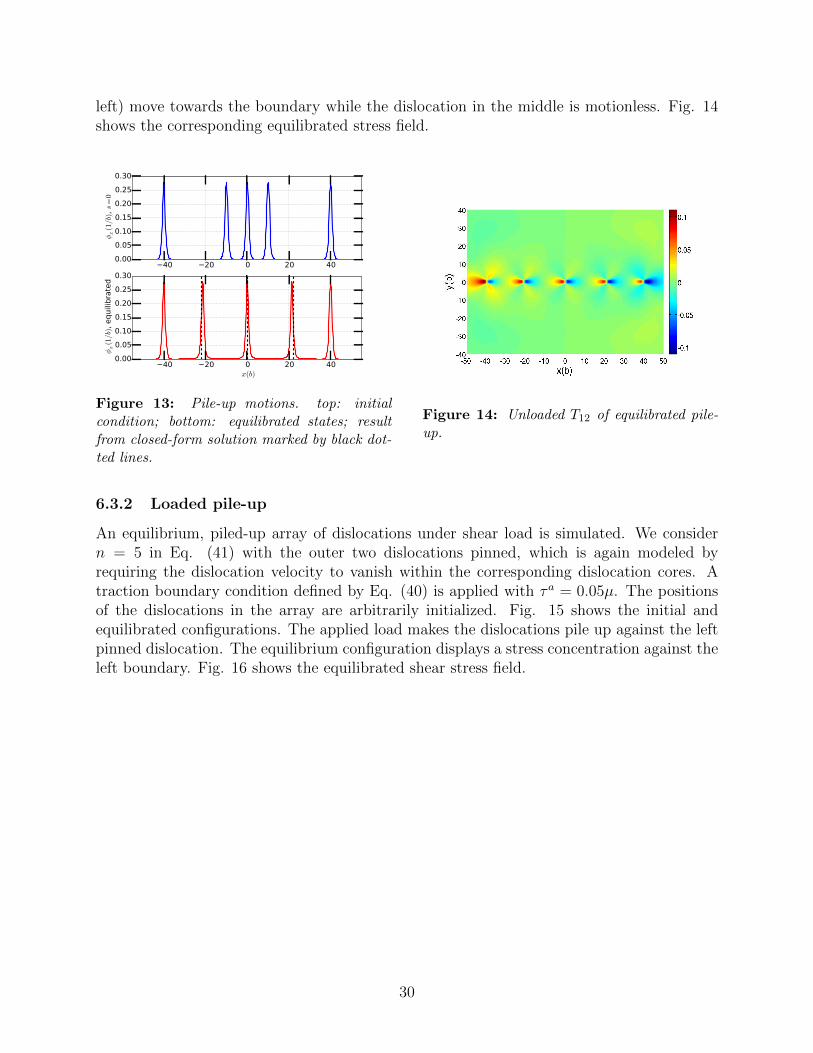
left) move towards the boundary while the dislocation in the middle is motionless. Fig. 14shows the corresponding equilibrated stress field.

40 20 0 20 400.00

0.05

0.10

0.15

0.20

0.25

0.30

φx(1/b

), s

=0

40 20 0 20 40 x(b)

0.00

0.05

0.10

0.15

0.20

0.25

0.30

φx(1/b

), e

quili

bra

ted

Figure 13: Pile-up motions. top: initialcondition; bottom: equilibrated states; resultfrom closed-form solution marked by black dot-ted lines.

Figure 14: Unloaded T12 of equilibrated pile-up.

6.3.2 Loaded pile-up

An equilibrium, piled-up array of dislocations under shear load is simulated. We considern = 5 in Eq. (41) with the outer two dislocations pinned, which is again modeled byrequiring the dislocation velocity to vanish within the corresponding dislocation cores. Atraction boundary condition defined by Eq. (40) is applied with τa = 0.05µ. The positionsof the dislocations in the array are arbitrarily initialized. Fig. 15 shows the initial andequilibrated configurations. The applied load makes the dislocations pile up against the leftpinned dislocation. The equilibrium configuration displays a stress concentration against theleft boundary. Fig. 16 shows the equilibrated shear stress field.

30

40 20 0 20 400.00

0.05

0.10

0.15

0.20

0.25

0.30 φx(1/b

), s

=0

40 20 0 20 40 x(b)

0.00

0.05

0.10

0.15

0.20

0.25

0.30

0.35

φx(1/b

), e

quili

bra

ted

Figure 15: Pile-up under shear. top: initialcondition; bottom: equilibrated states.

Figure 16: T12 of equilibrated pile-ups undershear load.

7 Dislocation motion in quasi-static deformations

In this section, we utilize our computational methodology to study the models described inSections (4.2) and (4.1). The context is phenomena related to dislocation motion when thematerial deformation may be nominally assumed as quasi-static.

7.1 Peierls Stress in Continuum Mechanics?

Applying a shear stress to a body sets an otherwise equilibrated dislocation under no loadin motion. The relation between the magnitude of the applied stress and the dislocationvelocity, as predicted by our models, is studied in this section, with particular empha-sis on exploring the question of whether a Peierls stress can exist within our models ofdislocation dynamics. The Peierls stress is the applied stress required to move a dislo-cation, and the question of its theoretical determination was first investigated by Peierls[Pei40] and improved by Nabarro [Nab47]. The improved model has since been calledthe Peierls model or the Peierls-Nabarro model4. Since then, this has been a vast areaof study with increasingly sophisticated models: at the continuum level with some notionof discreteness [LH59, Sch99, MBW98, Pic02], atomistic level with interatomic potentials[BJC+01, BCBK06, KBC12] and atomistic level with DFT input [LKBK00]. Such studieshave focused on energetic aspects since the problem intrinsically corresponds to very slow tovanishing rates of loading at macroscopic time scales. To our knowledge, the current state ofthe art of Molecular Dynamics simulations is not capable of effectively probing the possibleslow time scale dynamics that may be in play in this problem.

In the Peierls model, the existence of the Peierls stress arises from the change in totalenergy induced by a change in position of a dislocation (one assumes bodies of large enough

4Peierls also formulated and answered the question of the equilibrium profile of a non-singular, continu-ously distributed dislocation density field representative of a single isolated dislocation under no load in aninfinite body.

31

extent). In this sense, the Peierls stress is expected to vanish in any continuum mechani-cal model where the system energy is translationally-invariant, i.e., a dislocation is alwaysin ‘neutral equilibrium’ before the application of load, and will move under any (small)perturbation.

However, the Peierls model does not include the possibility of a moving dislocation profilechanging its shape, as it treats a dislocation as a rigid object (mathematically, a travelingwave) during motion. Clearly, if shape changes do occur on the application of load then,even by simply the logic of the Peierls model, it seems natural that the system energy canchange even at the onset of motion and thus have an effect on the question of existence of aPeierls stress in continuum models. This was our hypothesis, essentially based on energeticarguments, in studying the question within our continuum model. However, as we reportin Fig. 11, the matter is not simply dependent on energetics but also critically on the formof the evolution equation for φ that is a consequence of incorporating consideration of theconservation of Burgers vector on evolution.

We emphasize that the purpose of our study is not to deny the classical explanationof the Peierls stress arising from lattice discreteness; instead, it is to explore features ofa theoretical model of plausible material behavior in a systematic way and, in so doing,hopefully uncovering possible complementary mechanisms for the physical phenomenon.

Two important physical observations are in order here:

• An order-of-magnitude to keep in mind in this Section is that the expected Peierlsstress in FCC single crystals (a reasonable class of materials for comparison of ourresults) is ∼ 1MPa; translated in terms of the shear modulus, µ, of 26GPa adopted inour work, this amounts to ∼ 4× 10−5µ.

• The Peierls stress question is unequivocally a question of evolution, albeit extremelyslow (which in a sense makes the problem rather difficult to address by procedures thatattempt to resolve atomic vibrations). Thus, strictly, simply demonstrating a loadedand an unloaded single dislocation equilibria does not suffice, as it does not address thequestion of whether the loaded equilibrium is dynamically accessible from the unloadedequilibrium under the specified loading history. A quasi-static approximation may beadopted, but the equilibrium trajectory then needs to be justified as being acceptable,as discussed in Sec. 7.1.2.

The common simulation details used in this Section are listed in Table 3.

parameter name valuedomain width (W ) 110bdomain height (H) 90bNo. of elements 16320core-energy strength (ε) 0.25Young’s modulus (E) 70GPashear modulus (µ) 26GPaBurgers vector (b) 4.05× 10−10m

Table 3: Simulation details for Peierls stress problems.

32

7.1.1 Discrete mesh as surrogate for lattice discreteness effects

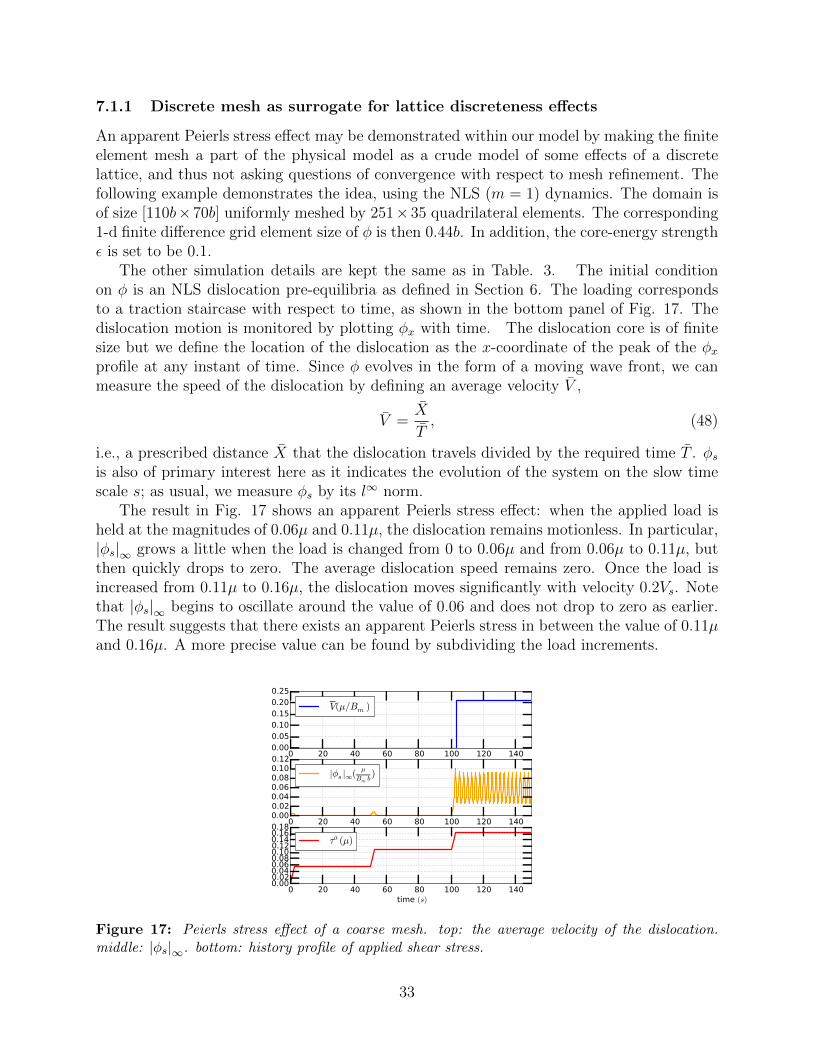
An apparent Peierls stress effect may be demonstrated within our model by making the finiteelement mesh a part of the physical model as a crude model of some effects of a discretelattice, and thus not asking questions of convergence with respect to mesh refinement. Thefollowing example demonstrates the idea, using the NLS (m = 1) dynamics. The domain isof size [110b×70b] uniformly meshed by 251×35 quadrilateral elements. The corresponding1-d finite difference grid element size of φ is then 0.44b. In addition, the core-energy strengthε is set to be 0.1.

The other simulation details are kept the same as in Table. 3. The initial conditionon φ is an NLS dislocation pre-equilibria as defined in Section 6. The loading correspondsto a traction staircase with respect to time, as shown in the bottom panel of Fig. 17. Thedislocation motion is monitored by plotting φx with time. The dislocation core is of finitesize but we define the location of the dislocation as the x-coordinate of the peak of the φxprofile at any instant of time. Since φ evolves in the form of a moving wave front, we canmeasure the speed of the dislocation by defining an average velocity V ,

V =X

T, (48)

i.e., a prescribed distance X that the dislocation travels divided by the required time T . φsis also of primary interest here as it indicates the evolution of the system on the slow timescale s; as usual, we measure φs by its l∞ norm.

The result in Fig. 17 shows an apparent Peierls stress effect: when the applied load isheld at the magnitudes of 0.06µ and 0.11µ, the dislocation remains motionless. In particular,|φs|∞ grows a little when the load is changed from 0 to 0.06µ and from 0.06µ to 0.11µ, butthen quickly drops to zero. The average dislocation speed remains zero. Once the load isincreased from 0.11µ to 0.16µ, the dislocation moves significantly with velocity 0.2Vs. Notethat |φs|∞ begins to oscillate around the value of 0.06 and does not drop to zero as earlier.The result suggests that there exists an apparent Peierls stress in between the value of 0.11µand 0.16µ. A more precise value can be found by subdividing the load increments.

0 20 40 60 80 100 120 1400.000.050.100.150.200.25

V(µ/Bm )

0 20 40 60 80 100 120 1400.000.020.040.060.080.100.12

|φs |∞(µ

Bm b)

0 20 40 60 80 100 120 140 time (s)

0.000.020.040.060.080.100.120.140.160.18

τa (µ)

Figure 17: Peierls stress effect of a coarse mesh. top: the average velocity of the dislocation.middle: |φs|∞. bottom: history profile of applied shear stress.

33

The value of the stress threshold is completely unrealistic (too high). Moreover, theapparent Peierls stress effect is only valid for this particular discrete mesh, and decreasesin a more refined mesh. As a practical device, an optimal mesh size could be associatedwith a target Peierls stress level in mind, in exploring problems where features of dislocationmechanics apart from the determination of Peierls stress is the subject of study.

Of course, our overriding goal in this paper is to explore the behavior of solutions toour pde model via numerical approximation. To this end, we strive to make statementsindependent of the mesh as demonstrated in Section 7.3.

7.1.2 Peierls stress effects for small Bm: the case of crystal dislocations

As already shown in Sections 6.1 and 6.1.1, the NGB model allows not only an unloadeddislocation equilibrium, but also a dislocation equilibrium with finite shear load up to 6.5×10−5µ. More importantly, the equilibrated dislocation is not moved by the shear load, butdeformed from its unloaded dislocation equilibrium shape.

Those solutions are obtained by solving for equilibria of (16). In particular, for the loadeddislocation equilibrium profile, we start with an initial guess corresponding to the NGB dis-location equilibrium (under no load) and use the Quasi-Newton method to obtain the loadeddislocation equilibrium solution, up to the tolerance specified in Eq. (38). Computationally,this procedure can be interpreted as the appropriate discrete analog of finding solutions tothe quasi-static system (22), i.e. following a trajectory on the equilibrium set, parametrizedby the applied load. We note here that this general philosophy is also adopted in latticestatics explorations of the Peierls stress. In computing these results, we use mesh B wherethe layer elements are of size 0.1 b. Additionally, the results are verified by convergence testsas discussed later in Sec. 7.3.

Thus, we conclude that our NGB dynamics displays a Peierls stress effect, subject tochecking that no untoward instability is observed on running the fast-scale dynamics (16)out of the initial state corresponding to the unloaded equilibrium dislocation when subjectedto load.

We want to check whether a small but finite load like 5× 10−5µ displaces the dislocationwhen inertia is involved. As dislocation motion is an inherently dissipative process, it isimportant that the loading mode for Peierls stress-related questions be such that externalenergy supply is available as the dislocation moves/evolves; applied, constant-in-time tractionloadings allow for this possibility and this is what we utilize in this Section.

Specifically, all simulations are performed in the following way. Initially, we obtain astate (φ0,u0) that satisfies equilibrium conditions for (16). φ0 and u0 are then used asinitial conditions of φ and u for Eqs. (16). A constant traction boundary condition definedby Eq. (40) with τa = 5× 10−5µ is applied. The dimensionless drag coefficient is chosen asBm = 0.0297. The other simulation details are grouped in Table. 3.

Instead of measuring dislocation velocity, another way to look closely at the differentdynamic characteristics exhibited by the three m cases is to measure an ‘instantaneousdislocation wave speed’ v defined in the following; this is the nondimensional analog of v inSec. 4. This measure is useful especially when the applied load and the dislocation motions

34

in x are small. For different m, v(x, t) takes the following form,

v(x, t) :=

− φx

Bm

[τ(x, t)− τ b(x, t) + εφxx(x, t)

], m = 0

− sgn(φx)

Bm

[τ(x, t)− τ b(x, t) + εφxx(x, t)

], m = 1

− 1

Bm

1

φx

[τ(x, t)− τ b(x, t) + εφxx(x, t)

]where φx 6= 0, m = 2.

(49)

vav(t) is calculated by summing v over the dislocation core at the specified time and dividingit by the core width. For our purposes here, the core width is chosen as 25 b which ismuch wider than the core defined in Fig. 5. We adopt this measure since the difference indislocation profiles corresponding to the various m dynamics is primarily at the very bottom,as already observed. We suspect that the v(x) distribution at the bottom of the dislocationprofile plays an essential role in determining dislocation motion (especially near the stepped‘core boundaries’ when such steps exist), and a width of 25 b allows us to capture thosefeatures in sufficient detail in the cases being considered here.

The motivation for the definition of v(x, t) is as follows: Suppose there exists a sufficientlysmooth function w that satisfies wt(x, t) = −wx(x, t)s(x, t). s(x, t) may depend on itsarguments through the values of the function w and its derivatives but since the latterare known, it is appropriate to think of s as a function directly of (x, t). Then, using anelementary argument of the method of characteristics, along a curve x(t) in (x, t) spacedefined by dx

dt= s(x, t) starting from a point x(t∗) = x0, the value of w is transported

unchanged, i.e. w(x(t), t) = w(x0, t∗). Thus at any instant of time, the transport velocity

s(x, t) may be interpreted as the instantaneous, local wave velocity at (x, t); a positive signof s(x, t) implies transport in the +x direction and a negative value implies transport in the−x direction. Admittedly, for m = 2 the definition of v(x, t) in (49) is somewhat artificial,but this is not central to the point we make subsequently.

We note that the fields φ and v in (10) satisfy the conditions outlined for w and s, mostlikely including the smoothness assumption (for sufficiently large ε).

We set up a simulation with initial condition being the unloaded NGB dislocation equi-librium of Fig. 5 with a constant-in-time applied load of 5 × 10−5µ. The dislocation staysmotionless. We plot φx(x) and v(x) along the layer in Fig.18. The v(x) profile obtained hereis definitely unfavorable to dislocation motion. The sign of v(x) on each side of the centre ofthe core indicates that the left side of the dislocation core tends to move to the right whilethe right side to the left, and the core bottom tends to spread out. The simulation lasts for0.4ns. This period is conservative since the NGL and NLS dynamics show motion withinthe first 0.05ns under the same applied load. It is shown in Fig. 18(a) that the dislocationstays motionless during this period. The v(x) profiles of Fig. 18 persist through out thesimulation. Due to the small time-period of simulation in this dynamic test, we furtherexamine the loaded NGB equilibrium as initial condition for the fast system. The appliedload is still 5× 10−5µ. The fast system is evolved for 0.42ns and the dislocation under loadshows no motion.

So far, based on the premise that

35

• if the quasi-static system displays a loaded dislocation equilibrium arrived at from anunloaded dislocation equilibrium state and

• the dynamic equations also validate that the unloaded dislocation equilibrium does notbegin to move under the action of the load on the fast time-scale,

then the system displays a Peierls stress, we have arrived at the following conclusions.

1. The NGB dynamics displays a Peierls stress effect for at least one initial condition (theunloaded NGB dislocation equilibrium). Interestingly, a curious ‘stochastic’ outcomearises out of our deterministic theory: two unloaded dislocation equilibria of verysimilar type at a gross level of reckoning (i.e. NLS and NGB dislocation equilibria)respond differently to loading and therefore predictions of Peierls stress for the NGBmodel may very well appear stochastic over repeated trials.

2. We have not been able to find a Peierls stress effect under load of the order of ∼10−5µ for any of the NGL, NLS, and NGB dynamics starting from the unloaded NGLdislocation equilibrium. We recall here that the results of Section 6.1 imply that theNGL and NLS quasi-static evolutions do not admit a loaded dislocation equilibrium(of the magnitude being discussed here) from their corresponding no-load dislocationequilibrium profiles as initial conditions.

60 40 20 0 20 40 60

x(b)

0

1

2

3

4

5

6

φx(1/b

)

1e 1

t=0−

t=0+

t≈0.125 ns

t≈0.25 ns

20 10 0 10 20

zoom into bottom

(a) φx

40 20 0 20 40

x(b)

1.5

1.0

0.5

0.0

0.5

1.0

1.5

−v(Vs)

1e 4

(b) v(x)

Figure 18: φx and v(x) of NGB dynamics. t = 0− stands for unloaded NGB equilibrium whichis used as initial condition. The instant of applying shear load 5 × 10−5µ is indicated by t = 0+.The dislocation shows no motion but slight shape change at bottom. v profile persists during thesimulation.

In the following, we explore the dynamic behaviours of the NGL, NLS, and NGB systemsunder load τa = 5×10−5µ, from a common initial condition of an unloaded NGL dislocationequilibrium shown in Fig. 5. The system runs on the fast time scale t = b/Vst and thesimulation runs for around 1 nanosecond.

36

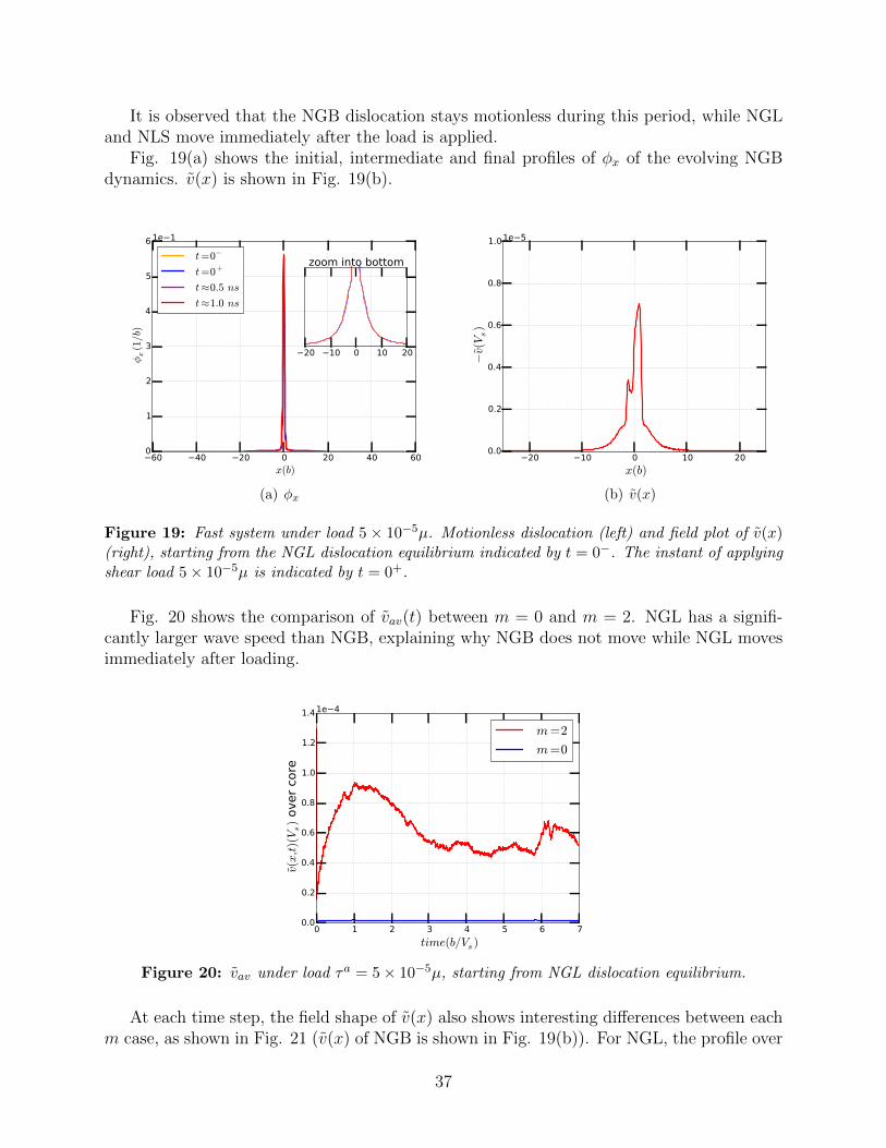
It is observed that the NGB dislocation stays motionless during this period, while NGLand NLS move immediately after the load is applied.

Fig. 19(a) shows the initial, intermediate and final profiles of φx of the evolving NGBdynamics. v(x) is shown in Fig. 19(b).

60 40 20 0 20 40 60

x(b)

0

1

2

3

4

5

6

φx(1/b

)

1e 1

t=0−

t=0+

t≈0.5 ns

t≈1.0 ns

20 10 0 10 20

zoom into bottom

(a) φx

20 10 0 10 20

x(b)

0.0

0.2

0.4

0.6

0.8

1.0

−v(Vs)

1e 5

(b) v(x)

Figure 19: Fast system under load 5× 10−5µ. Motionless dislocation (left) and field plot of v(x)(right), starting from the NGL dislocation equilibrium indicated by t = 0−. The instant of applyingshear load 5× 10−5µ is indicated by t = 0+.

Fig. 20 shows the comparison of vav(t) between m = 0 and m = 2. NGL has a signifi-cantly larger wave speed than NGB, explaining why NGB does not move while NGL movesimmediately after loading.

0 1 2 3 4 5 6 7

time(b/Vs )

0.0

0.2

0.4

0.6

0.8

1.0

1.2

1.4

v(x,t)(Vs)

over

core

1e 4

m=2

m=0

Figure 20: vav under load τa = 5× 10−5µ, starting from NGL dislocation equilibrium.

At each time step, the field shape of v(x) also shows interesting differences between eachm case, as shown in Fig. 21 (v(x) of NGB is shown in Fig. 19(b)). For NGL, the profile over

37

only the dislocation core area is plotted). It is observed that v at the dislocation boundariesof m = 2 and m = 1 are significantly larger than that of m = 0. Within the core, the peakof NGB is approximately 8 times less than the other two. This difference in v(x) contributesto the observed fact that NGB moves much slower than the NGL and NLS dislocations.

1.0 0.5 0.0 0.5 1.0

x(b)

0.0

0.2

0.4

0.6

0.8

1.0

−v(Vs)

1e 4

(a) m = 2

20 10 0 10 20

x(b)

0.0

0.2

0.4

0.6

0.8

1.0

−v(Vs)

1e 4

(b) m = 1

Figure 21: Field plot of v(x) of NGL and NLS under load 5×10−5µ, starting from NGL dislocationequilibrium.

It is instructive to compare the v profiles presented in Figures 18 and 21 for m = 0,under the load of 5× 10−5µ. Even though the dislocation stays motionless in the latter casefor the small time in which the observation has been done, the non-negative shape of thev(x) curve coupled with the inability to find a loaded dislocation equilibrium in quasi-staticequilibrium forces the conclusion that this situation reflects very slow motion of the type wediscuss in Section 7.1.4.

Fig. 22 provides a gross sense of the dislocation velocity versus applied load curves forthis regime of small loads. The results are gross because the exact governing equations inthis case should be (16); we use those equations, but with the assumption that for the smallmagnitude of loads and vanishing loading rates involved, material inertia is unimportant.From this real time dynamics with Bm = 1, the NGB dislocation does not show motionfor τa < 6.5 × 10−5µ. (Recall that a loaded dislocation equilibrium was also shown toexist for the quasi-static system (22)). The average velocity for the load of 2.5 × 10−4µ is5.99 × 10−5Vs. For these results, the time scale and the velocity are physically meaningful.The other simulation details are kept the same as in Table 3.

38

0.0 0.5 1.0 1.5 2.0 2.5

τa (µ) 1e 4

0

1

2

3

4

5

6

V(V

s)

1e 5

Figure 22: Dislocation velocity with respect to applied load at the threshold regime.

7.1.3 Preliminary parametric study of factors affecting the Peierls stress

• Effect of barrier height: We solve system (22) (with impulsively applied load), butnow with some lower barrier heights. That is, the function η in (13) is multiplied by afactor f ∈ (0, 1), and we consider the specific values

2

3,1

2,1

4

. (50)

The simulation details are kept the same as in Sec. 6. The tolerances specified by Eq.(38) remain in place. We find that f = 2

3is able to sustain both unloaded and loaded

equilibria. The Peierls stress is found to be around ∼ 5×10−5. (recall that f = 1 givesa Peierls stress 6.5 × 10−5µ; this load magnitude leads to non-convergence of |4u|∞for f = 2

3).

For f = 12

and f = 14, neither loaded nor unloaded equilibria can be attained.

• Effect of shape of η profile: With reference to Fig. 23, a function of the type form B(cf. [RBS92, Vit68, PDT10]), different from that specified in (13) represented as formA, is utilized. A Peierls stress of 7.5× 10−5µ is obtained for this case.

These results suggest, as expected, that the function η plays an essential role in theprediction of the Peierls stress in models like ours. Interestingly, we find that for each ofthese variations, dislocation pre-equilibria for the NGB dynamics can always be attained.

39

0.4 0.2 0.0 0.2 0.4 0.6 0.8 1.0 φ

4

3

2

1

0

1

2

3

4

5 η/

φ1e 1

form A

form B

(a) ∂η∂φ

0.4 0.2 0.0 0.2 0.4 0.6 0.8 1.0 φ

0.0

0.5

1.0

1.5

2.0

2.5

3.0

3.5

4.0

4.5

η

1e1

form A

form B

(b) η

Figure 23: Comparison of two types of η functions and their derivatives.

Finally, although our formulation is based on a small deformation theory, the resultantplastic strain can be substantial due to the value of φ = 0.5 corresponding to a well of thefunction η. In the following, we check whether an even larger plastic strain level, still specifiedby φ, can affect the Peierls stress results. We choose the value of φ = 1, corresponding to alattice invariant shear in a square lattice. The layer thickness is reduced to 1 b to maintainthe initial Burgers vector to be 1 b. The Peierls stress of this case is found to be ∼ 1×10−5µ.We again run a fast system (as described around Fig. 19) starting from unloaded NGBequilibrium for t ≈ 0.4ns under the same applied shear load 1 × 10−5µ. The dislocationstays motionless during the simulation.

7.1.4 Quasi-equilibrium aspects

In Section 6.1, we have hinted that the quasi-static dynamics of our equations (19) can showsluggish behavior practically indiscernible from equilibria, when judged solely on the meritof the rate of evolution of some obtained states that we have termed pre-equilibria.

In this section, we discuss some features of such (unloaded) dislocation pre-equilibriumstates and compare them with the states we have defined as unloaded dislocation equilibria(definitions in Section 6.1).

First, consider the dislocation pre-equilibria obtained from the common initial condition(37) (and utilized for the result in Figure 5). Specifically, we make the following observations:

1. Initially, the three quasi-static systems (19) (corresponding to m = 0, 1, 2) evolve fromthe initial condition (37) with significant shape changes of φx and rates of change |φs|∞.The profiles of φx then settle on the dislocation pre-equilibria configurations with thecorresponding |φs|∞ decreasing to 5× 10−5.

2. The displacement fields u corresponding to these dislocation pre-equilibria appear tohave no discernible differences from their corresponding dislocation equilibrium dis-placement profiles. However, the difference in stress fields are on the scale of 10−4µ.

40

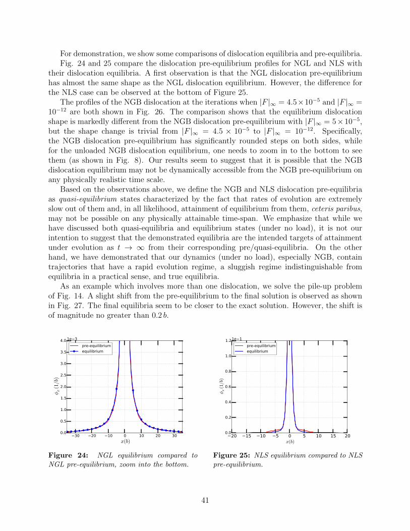
For demonstration, we show some comparisons of dislocation equilibria and pre-equilibria.Fig. 24 and 25 compare the dislocation pre-equilibrium profiles for NGL and NLS with

their dislocation equilibria. A first observation is that the NGL dislocation pre-equilibriumhas almost the same shape as the NGL dislocation equilibrium. However, the difference forthe NLS case can be observed at the bottom of Figure 25.

The profiles of the NGB dislocation at the iterations when |F |∞ = 4.5×10−5 and |F |∞ =10−12 are both shown in Fig. 26. The comparison shows that the equilibrium dislocationshape is markedly different from the NGB dislocation pre-equilibrium with |F |∞ = 5×10−5,but the shape change is trivial from |F |∞ = 4.5 × 10−5 to |F |∞ = 10−12. Specifically,the NGB dislocation pre-equilibrium has significantly rounded steps on both sides, whilefor the unloaded NGB dislocation equilibrium, one needs to zoom in to the bottom to seethem (as shown in Fig. 8). Our results seem to suggest that it is possible that the NGBdislocation equilibrium may not be dynamically accessible from the NGB pre-equilibrium onany physically realistic time scale.

Based on the observations above, we define the NGB and NLS dislocation pre-equilibriaas quasi-equilibrium states characterized by the fact that rates of evolution are extremelyslow out of them and, in all likelihood, attainment of equilibrium from them, ceteris paribus,may not be possible on any physically attainable time-span. We emphasize that while wehave discussed both quasi-equilibria and equilibrium states (under no load), it is not ourintention to suggest that the demonstrated equilibria are the intended targets of attainmentunder evolution as t → ∞ from their corresponding pre/quasi-equilibria. On the otherhand, we have demonstrated that our dynamics (under no load), especially NGB, containtrajectories that have a rapid evolution regime, a sluggish regime indistinguishable fromequilibria in a practical sense, and true equilibria.

As an example which involves more than one dislocation, we solve the pile-up problemof Fig. 14. A slight shift from the pre-equilibrium to the final solution is observed as shownin Fig. 27. The final equilibria seem to be closer to the exact solution. However, the shift isof magnitude no greater than 0.2 b.

30 20 10 0 10 20 30

x(b)

0.0

0.5

1.0

1.5

2.0

2.5

3.0

3.5

4.0

φx(1/b

)

1e 3

pre-equilibrium

equilibrium

Figure 24: NGL equilibrium compared toNGL pre-equilibrium, zoom into the bottom.

20 15 10 5 0 5 10 15 20 x(b)

0.0

0.2

0.4

0.6

0.8

1.0

1.2

φx(1/b)

1e 1

pre-equilibrium

equilibrium

Figure 25: NLS equilibrium compared to NLSpre-equilibrium.

41

20 15 10 5 0 5 10 15 20 x(b)

0.0

0.5

1.0

1.5

2.0

2.5

3.0 φx(1/b)

1e 1

|F|∞=5×10−5

|F|∞=4.5×10−5

|F|∞=10−12

Figure 26: Comparison of NGB pre-equilibrium (5×10−5) and two moments duringNewton iterations. NGB equilibrium is resolvedto |F |∞ = 10−12.

40 20 0 20 40 x(b)

0.0

0.5

1.0

1.5

2.0

2.5

3.0

3.5

φx(1/b)

1e 1

pre-equilibrium

equilibrium

Figure 27: Pre-equilibrium compared to equi-librium of unloaded pile-ups. The black dottedlines indicate the analytical solutions.

7.1.5 Peierls stress effects for Bm 1

We now consider dislocation motion in the presence of large drag. The question is whetherone can still observe the Peierls stress effect on a slow time scale characterized by the largedrag, under a slow loading rate.

The governing equations for Bm 1 are (19). The system runs on the slow time scaledetermined by the non-dimensional drag number Bm. Here, the time scale and velocities areall physically meaningful. We implement a series of simulations with applied stress startingfrom τa = 5× 10−5. The increments of applied load are kept very small especially when theloads are within 5× 10−3µ.

The simulation set-up is kept the same as in Section 7.1.2, with parameters listed inTable 1. We consider all three NGB (m = 0), NLS (m = 1) and NGL (m = 2) cases, withparticular interest in the NGB (m = 0) case, since it is derived from the simplest kineticassumption, and also because we have shown the Peierls stress effect for this dynamics insection 7.1.2 where Bm is small.

The unloaded, dislocation pre-equilibrium profiles of Fig. 24, 25 and 26 are used asinitial conditions for each m dynamics. Uniform-in-time shear traction boundary conditions,as described in Eq. (40) are imposed. The average velocity V is measured by (48); X isconservatively chosen as 0.1 b. The dislocation motion is thus quantified by measuring Vand |φs|∞. In addition, we define a ‘slowness,’ S := V −1, to help visualize the Peierls stresseffect.

The results are shown in Fig. 28(a) where V is plotted for applied loads smaller than0.001µ. The corresponding slowness data S is shown in Fig. 28(b). A direct observation isthat the dislocation has much slower motion with increasing m. The slowing down causedby m is clearly demonstrated by fitting S to a power law. We have fit S vs. applied stressfor the whole range of stresses below 5× 10−3µ based on the data of τa > 5× 10−5, since thedislocation for NGB under load 5× 10−5 does not show any motions during the simulation.

42

The plots of Fig. 28(a) and Fig. 28(b) display only the parts of that curve at the lowerend of the spectrum - the fit is uniformly good in the entire range of stresses. The NGB(m = 0) dynamics has an exponent of 1.24, much larger than that for NLS (m = 1) and NGL(m = 2). Since we are not able to perform infinitely-long time simulations, the conclusion isthat the NGB dynamics starting from different NGL and NGB equilibrated profiles all showno or extremely slow motions.

0 1 2 3 4 5 6 7 8

τa (µ) 1e 4

0.0

0.5

1.0

1.5

2.0

2.5

3.0

3.5

4.0

V(µ/B

m)

1e 3

m=2

m=1

m=0

(a) zoom in view

0 1 2 3 4 5 6 7 8

τa (µ) 1e 4

0.0

0.5

1.0

1.5

2.0

2.5

3.0

3.5

4.0

4.5

S(1/V

s)

1e5

S=1.98/τ1.24

S=1.10/τ0.99

S=0.29/τ0.95

(b) slowness

Figure 28: Velocity and slowness recorded from simulations.

The existence of a Peierls stress in this Bm 1 regime would be justified if S → ∞for a non-zero value of applied stress. We are unable to access smaller loads than shownbecause of the prohibitive time taken by these very long-time simulations. However, basedon the power law fits of the available data, it can be quantitatively concluded that for theNGB dynamics both V (0) = 0 and dV

dτa(0) = 0. For the NLS (m = 1) dynamics, the

derivative may be considered a constant (making allowances for fitting), whereas for theNGL (m = 2) dynamics, dV

dτa(0)→∞. In addition, we show the plots of v(x) and vav(t) for

the NGB simulation of this section under load 5×10−5µ. We conclude that in all probabilitythere exists a Peierls stress effect in the NGB dynamics for Bm 1 based on the followingobservations:

1. Fig. 29(a) shows that the NGB dynamics has a v profile not favourable to dislocationmotions, for the same reason as discussed around Fig. 18.

2. There is an obvious decreasing trend in vav (Fig. 29(b)). The value of vav at s = 3000is around 1/20 of that at s = 0. This suggests that the evolution of φ (specifically inx direction) is slowing down.

3. Recall that we chose 0.1 b for X in determining the average velocity (48) - this is inpart dictated by the extended times for which these simulations have to be run. Thisis a conservative choice and it is reasonable to expect the possibility of S → ∞ for

43

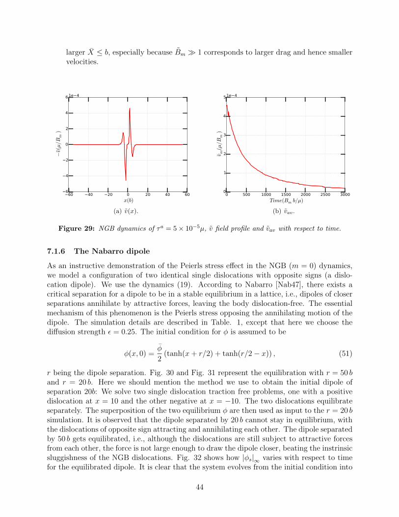
larger X ≤ b, especially because Bm 1 corresponds to larger drag and hence smallervelocities.

60 40 20 0 20 40 60

x(b)

6

4

2

0

2

4

6

−v(µ/B

m)

1e 4

(a) v(x).

0 500 1000 1500 2000 2500 3000

Time(Bm b/µ)

0

1

2

3

4

5

vav(µ/B

m)

1e 4

(b) vav.

Figure 29: NGB dynamics of τa = 5× 10−5µ, v field profile and vav with respect to time.

7.1.6 The Nabarro dipole

As an instructive demonstration of the Peierls stress effect in the NGB (m = 0) dynamics,we model a configuration of two identical single dislocations with opposite signs (a dislo-cation dipole). We use the dynamics (19). According to Nabarro [Nab47], there exists acritical separation for a dipole to be in a stable equilibrium in a lattice, i.e., dipoles of closerseparations annihilate by attractive forces, leaving the body dislocation-free. The essentialmechanism of this phenomenon is the Peierls stress opposing the annihilating motion of thedipole. The simulation details are described in Table. 1, except that here we choose thediffusion strength ε = 0.25. The initial condition for φ is assumed to be

φ(x, 0) =φ

2(tanh(x+ r/2) + tanh(r/2− x)) , (51)

r being the dipole separation. Fig. 30 and Fig. 31 represent the equilibration with r = 50 band r = 20 b. Here we should mention the method we use to obtain the initial dipole ofseparation 20b: We solve two single dislocation traction free problems, one with a positivedislocation at x = 10 and the other negative at x = −10. The two dislocations equilibrateseparately. The superposition of the two equilibrium φ are then used as input to the r = 20 bsimulation. It is observed that the dipole separated by 20 b cannot stay in equilibrium, withthe dislocations of opposite sign attracting and annihilating each other. The dipole separatedby 50 b gets equilibrated, i.e., although the dislocations are still subject to attractive forcesfrom each other, the force is not large enough to draw the dipole closer, beating the instrinsicsluggishness of the NGB dislocations. Fig. 32 shows how |φs|∞ varies with respect to timefor the equilibrated dipole. It is clear that the system evolves from the initial condition into

44

an equilibrium state, for all practical purposes at least. The equilibrated dipole results in astatic stress field as shown in Fig. 33.

40 20 0 20 400.3

0.2

0.1

0.0

0.1

0.2

0.3

φx(1/b

)

s=0

40 20 0 20 40 x(b)

0.3

0.2

0.1

0.0

0.1

0.2

0.3

φx(1/b

)

s=3000

Figure 30: Equilibrated separated dipole.

40 20 0 20 400.3

0.2

0.1

0.0

0.1

0.2

0.3

φx(1/b

)

s=0

40 20 0 20 40

x(b)

0.3

0.2

0.1

0.0

0.1

0.2

0.3

φx(1/b

)

s=3000

Figure 31: Annihlated dislocation dipole.

0 500 1000 1500 2000 2500

time(Bmb/µ)

0.0

0.2

0.4

0.6

0.8

1.0

1.2

1.41e 3

|φs |∞(µ

Bm b)

Figure 32: |φs|∞ of equilibriated dipole. Figure 33: σ12 of equilibrated dipole.

Applying a large enough shear load counterbalances the attractive Peach-Koehler forcesand expands the dipole. Fig. 34 shows a series of snapshots of that scenario.

45

(a) (b) (c)

Figure 34: Dipole expands under shear stress.

7.1.7 Idealized dislocation dissociation5

Energy considerations dictate that it is possible for a dislocation to dissociate (split) into apair, with the Burgers vectors of the dislocations in the pair adding up to that of the originaldislocation. The argument from the classical theory essentially amounts to the following:Consider a large enough body containing, in the first instance, a single straight dislocationof Burgers vector magnitude b and in the second instance two dislocations of the same signas in the first case separated by a distance R, but each of Burgers vector magnitude 1

2b. We

now wish to compare the total energies of the two configurations; in the linear theory this isa question of comparing infinite magnitudes (even for finite bodies). Nevertheless, with theusual hand-waving of the linear theory related to accounting for the core energy, if in the first

case the energy is written as ab2 then in the second case the energy is 2a(

12b)2

+ c b2

R, where

a, c are positive constants. For R sufficiently large, the energy of the second configurationis smaller than the first; therefore, dissociation is favored. Such a phenomenon is actuallyobserved in closed-packed crystals with low stacking fault energy. We show in this sectionthat, without any additional constitutive rules, our model is able to simulate an idealizeddislocation dissociation process.

We use the NGB dynamics and keep the simulation details as for calculations reportedin Fig. 5 with the following modifications:

φ(x, t = 0) = φ tanh(ax)

ε = 0.025, a =√µ/4ε,

(52)

which represents an initial dislocation with a Burgers vector magnitude of 2b. Fig. 35 showsthe process of it splitting into two separated dislocations, each of Burgers vector magnitudeb. The corresponding re-distribution of plastic strain caused by the dislocation dissociation isalso shown. In this way, it locally minimizes the total system energy. The initial dislocationprofile spans three successive wells of η (to achieve its Burgers vector magnitude), and weobserve from the simulation that each dislocation in the dissociated pair spans two wells ofη as they move apart. The separated single dislocations have repulsive forces in between,and push each other away after dissociation.

5We thank Mr. Chiqun Zhang for his help with the simulations in this Section.

46

40 20 0 20 40

x(b)

0.0

0.5

1.0

1.5

2.0

φx(1/b)

s=0

s=15

s=100

s=200

s=300

(a) φx

40 20 0 20 40

x(b)

4

2

0

2

4

φ

1e 1

s=0

s=15

s=100

s=200

s=300

(b) φ

Figure 35: An example of modeling dislocation dissociation.

7.2 Loading and unloading of a single dislocation

Here we show the response of the model to a loading-unloading cycle. We continue to usethe slow dynamics (19). We apply a simple shear traction boundary condition (40) to movethe dislocation from its equilibrated position. The load is then instantaneously removed.The NGB dynamics shows interesting/peculiar behavior as presented in Fig. 36(a) at threecritical moments during the simulation: the top, where s = 0, the dislocation is equilibrated.The middle panel shows the dislocation driven to its furthest location, and at that momentthe load suddenly drops to zero. Without any exterior stress, the dislocation spike creepsbackwards with diminishing speed to finally equilibrate at the position shown in the bottompanel. The equilibrium shape is similar to the shape at the start with some differences;we have not let the equilibration process run long enough to conclude whether the heightof the peak returns to the original value or not. As can be seen, the equilibrium shape ofthe dislocation is significantly different from that during motion. The history of |φs|∞ onthe right also reflects this process: the sudden increase of |φs|∞ is caused by the suddenload drop. After unloading, |φs|∞ decreases sharply, which suggests the re-(pre)equilibrationprocess of the load-free dislocation. In contrast, the unloading behaviour of the NLS (m = 1)and the NGL (m = 2) dislocations are different. There, the dislocations continue to movetowards the left boundary after the load is taken away, presumably due to the attractionof the free boundary. While the recoil of the NGB dislocation gives us some pause in thecontext of expected behaviour based on classical ideas, its equilibration is another exampleof the Peierls stress effect in the NGB case. We have checked that if an NGB dislocationunder no load is placed closer to the boundary, it does move towards the boundary. We havealso checked that for all three NGL, NLS, and NGB dislocations, the core-averaged layerstresses are positive, indicating an attraction towards the left boundary.

47

40 20 0 20 400.00.10.20.30.40.5

φx(1/b

) s=0

40 20 0 20 400.00.10.20.30.40.5

φx(1/b

) unload

40 20 0 20 40

x(b)

0.00.10.20.30.40.50.6

φx(1/b

) equilibrated

(a) Motion of a dislocation under loading-unloading.top: free traction equilibrium ready to move. middle:dislocation moves to the left most when load is droppedto zero. bottom: dislocation moves back and re-gainsits new equilibrium state.

0 1000 2000 3000 4000 5000 6000 7000 8000

Time (Bmb/µ)

0

1

2

3

4

5

6

71e 3

|φs |∞(µ

Bmb)

(b) |φs|∞ corresponding to (a)

Figure 36: Loading then unloading (m = 0).

40 20 0 20 400.00.10.20.30.40.5

φx(1/b

) s=0

40 20 0 20 400.00.10.20.30.40.50.6

φx(1/b

) unload

40 20 0 20 40

x(b)

0.00.10.20.30.40.50.6

φx(1/b) s=1500

(a) loading then unloading of m = 1.

40 20 0 20 400.00.10.20.30.40.5

φx(1/b

) s=0

40 20 0 20 400.00.10.20.30.40.50.6

φx(1/b

) unload

40 20 0 20 40

x(b)

0.00.10.20.30.40.50.6

φx(1/b) s=1500

(b) loading then unloading of m = 2.

Figure 37: Loading then unloading (m = 1, 2). The dislocations moves to the left under simpleshear traction same as m = 0. However, as the load is removed, m = 1 and m = 2 both keep movingto the left boundary. Specifically, NGL moves faster than NLS as shown in the bottom snapshot atthe same nondimensional time s = 5500.

7.3 Convergence Test

The Peierls stress results are verified by convergence tests. First, we take an NLS (m = 1)system with applied load τa = 0.005µ from Section 7.1.5 and show convergence with respect

48

to the mesh of |φs|∞, the dislocation displacement, and the average speed V . These threemeasurements together quantify the motion of a dislocation. All the simulation details canbe found in Table. 1. The use of transition elements around the layer keeps the overallcomputation time from growing significantly as the layer gets refined. Let h denote thewidth of layer elements and we create meshes with h = 0.2, 0.1, 0.05, 0.025(b). We shouldalso point out that the finite difference grid is refined accordingly in the meantime and thetime steps are automatically refined according to Eq. (27). Although convergence of |φs|∞is a more stringent test than the other two, even in Fig. 38(a), one can observe the trendof convergence of |φs|∞ with decreasing h. Fig. 38(b) shows the position of the dislocationpeak X vs. s. Processing Fig. 38(b) by dividing X with time gives the averaged speed V .As shown in 38(c), V converges with h, but with a notable disturbance when X < 0.5b forall h.

0 500 1000 1500 2000 2500 3000

normalized time (Bm b/µ)

1.20

1.25

1.30

1.35

1.40

1.45

1.50

1.55

1.60

|φs| ∞

(µ

Bmb)

1e 3

h=0.2 b

h=0.1 b

h=0.05 b

h=0.025 b

(a) |φs|∞

0 500 1000 1500 2000 2500 3000

normalized time (s)

0

2

4

6

8

10

12

14

16

x c

oord

inate

of α

peak

h=0.2 b

h=0.1 b

h=0.05 b

h=0.025 b

(b) dislocation position

0.5 1.0 1.5 2.0 2.5 3.0 3.5 4.0

X(b)

0.000

0.005

0.010

0.015

0.020

V(µ/Bm

)

h=0.2 b

h=0.1 b

h=0.05 b

h=0.033 b

h=0.025 b

(c) V

Figure 38: Convergence test.

For the equilibrium results obtained with the Quasi-Newton scheme, we run the same

49

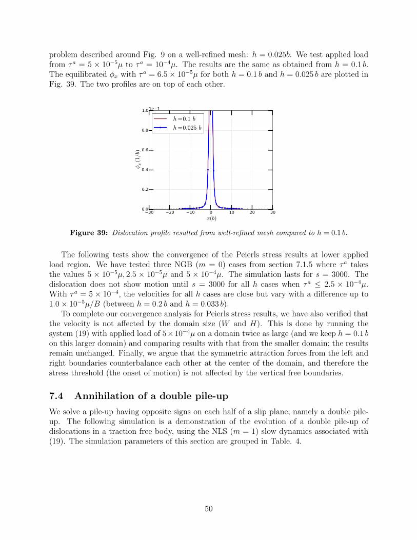
problem described around Fig. 9 on a well-refined mesh: h = 0.025b. We test applied loadfrom τa = 5 × 10−5µ to τa = 10−4µ. The results are the same as obtained from h = 0.1 b.The equilibrated φx with τa = 6.5× 10−5µ for both h = 0.1 b and h = 0.025 b are plotted inFig. 39. The two profiles are on top of each other.

30 20 10 0 10 20 30

x(b)

0.0

0.2

0.4

0.6

0.8

1.0

φx(1/b)

1e 1

h=0.1 b

h=0.025 b

Figure 39: Dislocation profile resulted from well-refined mesh compared to h = 0.1 b.

The following tests show the convergence of the Peierls stress results at lower appliedload region. We have tested three NGB (m = 0) cases from section 7.1.5 where τa takesthe values 5 × 10−5µ, 2.5 × 10−5µ and 5 × 10−4µ. The simulation lasts for s = 3000. Thedislocation does not show motion until s = 3000 for all h cases when τa ≤ 2.5 × 10−4µ.With τa = 5 × 10−4, the velocities for all h cases are close but vary with a difference up to1.0× 10−5µ/B (between h = 0.2 b and h = 0.033 b).

To complete our convergence analysis for Peierls stress results, we have also verified thatthe velocity is not affected by the domain size (W and H). This is done by running thesystem (19) with applied load of 5×10−4µ on a domain twice as large (and we keep h = 0.1 bon this larger domain) and comparing results with that from the smaller domain; the resultsremain unchanged. Finally, we argue that the symmetric attraction forces from the left andright boundaries counterbalance each other at the center of the domain, and therefore thestress threshold (the onset of motion) is not affected by the vertical free boundaries.

7.4 Annihilation of a double pile-up

We solve a pile-up having opposite signs on each half of a slip plane, namely a double pile-up. The following simulation is a demonstration of the evolution of a double pile-up ofdislocations in a traction free body, using the NLS (m = 1) slow dynamics associated with(19). The simulation parameters of this section are grouped in Table. 4.

50

parameter name valuedomain width (W ) 220bdomain height (H) 180bNo. of elements 33960No. of nodes 34038core-energy strength (ε) 0.25Young’s modulus (E) 70GPashear modulus (µ) 26GPaBurgers vector (b) 4.05× 10−10mShear wave speed (Vs) Vs = 3.13 km/s

Table 4: Simulation details for double annihilation pile-up.

n = 14 dislocation spikes are initialized at s = 0, spaced by 5b, i.e., the ith dislocation has apeak at xi = (−35 + 5i)b, 0 ≤ i ≤ n.

As the system evolves, the inner dislocations are drawn closer immediately and annihilateunder the combined effects of attractive forces (of dislocations of opposite signs) and repulsiveforce (of dislocations of the same sign). The motions of others are driven by a complex time-dependent stress field. Fig. 40 shows the trajectories of each dislocation in this process. Notethat the outside two trajectories spread outwards initially before bending and becomingparallel in the end due to the annihilation of all the other dislocations. The two outerdislocations are separated by 132b at the moment that all other dislocations annihilate asshown in the scenario of Fig. 31. Their evolution towards each other becomes extremely slowdue to the small magnitude of the attraction force between them due to the large distance ofseparation. Also, the boundary attractions are extremely small based on the analysis aroundFig. 37(a).

0

100

200

300

400

−120−80

−400

4080

120

−1

0

1

x(b)

Time step(Bb/µ)

φ x (1/

b)

Figure 40: Double pile-up in traction freebody.

60 40 20 0 20 40 602.01.51.00.50.00.51.01.52.0

φx(1/b

), s

=0

60 40 20 0 20 40 60 x(b)

2.01.51.00.50.00.51.01.52.0

φx(1/b

), |φ

x| ∞≈

0

Figure 41: Almost completely continuous dou-ble pile-up with ends fixed (top). The middledislocations annihilate (bottom).

By inserting more dislocations into the previous array, one could simulate almost contin-uously distributed pile-ups. The outer two dislocations on both sides are pinned. We use a

51

[110b× 90b] domain for this case. The initial distribution of dislocations is shown in the toppanel of Fig. 41. All the other simulation details are kept the same as in Table. 4. Fig. 41bottom shows the final state of the double pile-ups. It shows that all dislocations annihilateexcept the pinned ones on the outside. This example also demonstrates that although α isa conserved variable, the norm of α is not. There exist several continuum dislocation plas-ticity models (motivated from discrete dislocation methodology) that insist on conservationof both α and norm of α, while this is a straightforward counterexample.

8 Dislocation motion in dynamic deformations

In this section we examine the capability of our theory of modeling dislocation-related phe-nomena in the presence of material inertia. In all instances, the system (16) constitutes thegoverning equations. The theory has modeling relevance for phenomena at the atomic aswell as geologic length scales. With computational capabilities of the type demonstratedin this paper, our theory appears to be a relatively straightforward and robust tool toprobe such questions in fair generality that otherwise require delicate analytical skills (cf.[Wil65, Mur63, AR02, Fre98, Mar11, Pel10, Pel11]).

8.1 Subsonic, intersonic, and supersonic dislocation motion

We investigate dislocation velocity versus applied load phenomena in a specific setting, withspecial interest in probing the sub-inter-supersonic regime of dislocation motion within ourmodel. Because of the peculiar singularities at the speed of sound that occur in the relativelyfew complete solutions available in the linear elastic theory of dislocations, e.g. [AR02], ques-tions of supersonic dislocation motion have generally been outside the realm of explorationfor the classical theory of dislocations. Of course, if it is assumed that a stress wave in apurely linear elastic medium is the only carrier of signals that fail the material to form adislocation core, then it is indeed physically unreasonable to expect the core to be able totravel faster than the linear elastic wave speeds of the material.

However, a system of numerical experiments performed by Gumbsch and Gao [GG99],motivated by transonic shear cracks observed in high-speed impacts [RSC99], reported thepossibility of a transonic dislocation speeding up into the supersonic regime in a highly pre-stressed body. The MD experiment studied the motion of dislocations nucleated within athin strip subjected to simple shear pre-strain. The dislocation velocity varies from subsonicto supersonic magnitudes according to the level of enforced strains.

A sketch of the MD velocity vs. applied shear strain obtained in Gumbsch and Gao’sMD experiments is shown in Fig. 42. In the sketch, only the black dots are of concern sinceour problem is slightly different from theirs; e.g. the MD experiment involves the process ofdislocation nucleation from a notch tip. The velocity data has two sudden transitions closeto the shear wave and pressure wave velocity Vs and Vp. The very nonlinear velocity vs.applied strain relationship is also noteworthy. The objective of this section is to qualitativelycompare the results from our model with these MD results. To this end, we set up the initial-boundary value problem in a manner similar in principle to the MD simulations in [GG99].The model has a domain of size 110b×80b, discretized uniformly. The simulation parameters

52

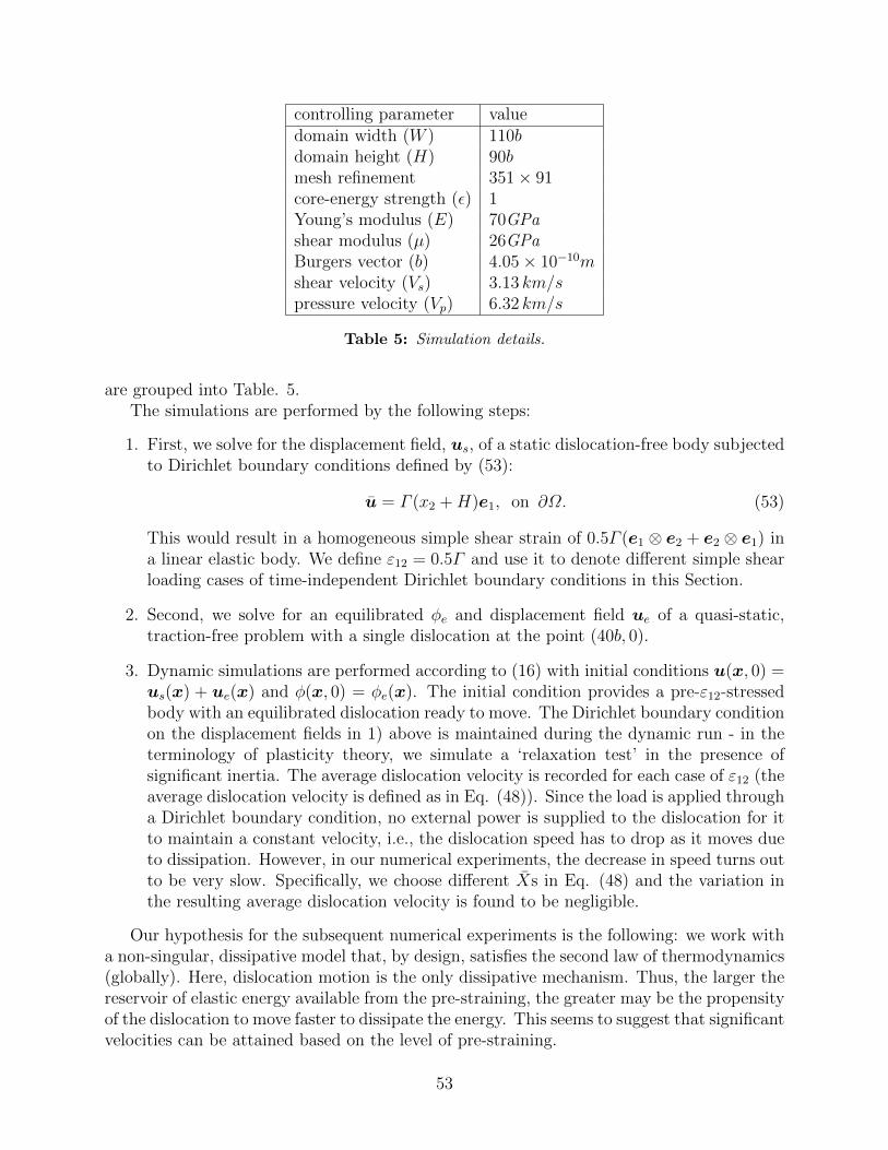
controlling parameter valuedomain width (W ) 110bdomain height (H) 90bmesh refinement 351× 91core-energy strength (ε) 1Young’s modulus (E) 70GPashear modulus (µ) 26GPaBurgers vector (b) 4.05× 10−10mshear velocity (Vs) 3.13 km/spressure velocity (Vp) 6.32 km/s

Table 5: Simulation details.

are grouped into Table. 5.The simulations are performed by the following steps:

1. First, we solve for the displacement field, us, of a static dislocation-free body subjectedto Dirichlet boundary conditions defined by (53):

u = Γ (x2 +H)e1, on ∂Ω. (53)

This would result in a homogeneous simple shear strain of 0.5Γ (e1 ⊗ e2 + e2 ⊗ e1) ina linear elastic body. We define ε12 = 0.5Γ and use it to denote different simple shearloading cases of time-independent Dirichlet boundary conditions in this Section.

2. Second, we solve for an equilibrated φe and displacement field ue of a quasi-static,traction-free problem with a single dislocation at the point (40b, 0).

3. Dynamic simulations are performed according to (16) with initial conditions u(x, 0) =us(x) + ue(x) and φ(x, 0) = φe(x). The initial condition provides a pre-ε12-stressedbody with an equilibrated dislocation ready to move. The Dirichlet boundary conditionon the displacement fields in 1) above is maintained during the dynamic run - in theterminology of plasticity theory, we simulate a ‘relaxation test’ in the presence ofsignificant inertia. The average dislocation velocity is recorded for each case of ε12 (theaverage dislocation velocity is defined as in Eq. (48)). Since the load is applied througha Dirichlet boundary condition, no external power is supplied to the dislocation for itto maintain a constant velocity, i.e., the dislocation speed has to drop as it moves dueto dissipation. However, in our numerical experiments, the decrease in speed turns outto be very slow. Specifically, we choose different Xs in Eq. (48) and the variation inthe resulting average dislocation velocity is found to be negligible.

Our hypothesis for the subsequent numerical experiments is the following: we work witha non-singular, dissipative model that, by design, satisfies the second law of thermodynamics(globally). Here, dislocation motion is the only dissipative mechanism. Thus, the larger thereservoir of elastic energy available from the pre-straining, the greater may be the propensityof the dislocation to move faster to dissipate the energy. This seems to suggest that significantvelocities can be attained based on the level of pre-straining.

53

Additionally, the following analysis6 shows the possibility of supersonic stress waves in

an initially stressed body in the context of linearized elasticity. Let P , τ andτ be the first

Piola-Kirchhoff stress, the Kirchhoff stress and the contravariant convected rate of Kirchhoffstress, defined with respect to an initially stressed configuration (treated as the currentconfiguration). Then, P evaluated at the current configuration is given by

P = τF−T − τLTF−T

= τ − τLT

=τ +Lτ + τLT − τLT

=τ +Lτ .

Balance of linear momentum on the current configuration can be written as

div[τ +Lτ

]= ρv,

and we assume the elastic constitutive relationship

τ = C : D,

where C is the 4th order linear elasticity tensor and D = 12

(L+LT

). Let Mijkl = Cijkl +

τljδik. Assuming plane-wave solutions of the form vi = pieI(nrxr−ct), where p is the velocity

mode of the plane wave (polarization), n the direction of propagation of the velocity wave,and I =

√−1, one has the characteristic equation[

Mijklnlnj − ρc2δik]pk = 0

for the speed(s) c and polarization p. Choosing now a homogeneous state of initial stressgiven by τ = τa⊗b with a and b as arbitrary unit vectors, one finds that longitudinal waves(p = n) propagate with speed

cL =

√λ+ 2µ+ τ(a · n)(b · n)

ρ

and transverse waves (p in plane normal to n) propagate with speed

cT =

√µ+ τ(a · n)(b · n)

ρ.

Note that the linear elasticity analogs of cL and cT are Vp =√

λ+2µρ

and Vs =√

µρ. Thus

cL > Vp > Vs as well as cT > Vp > Vs are definite possibilities for suitable states of initialstress, even without resorting to full-blown nonlinear theory.

6We acknowledge discussions with Profs. C. S. Man and R. W. Ogden on the possibility of elastic wavesin linearized elasticity supersonic with respect to linear elasticity.

54

0.02 0.04 0.06 0.08 0.10

homogeneous shear strain ε12

0

1

2

3

4

5

6

7

avera

ge d

islo

cati

on v

elo

city

(km/s)

Vs

Vp

subsonic

transonic

supersonic

Figure 42: Sketch of the MD results from Gumbsch and Gao [GG99], reprinted with permissionfrom AAAS. Dashed lines indicate relevant acoustic wave speeds.

8.1.1 Linear Elasticity

The dynamic simulations discussed above are performed with the equations (16), utilizingthe constitutive equation (12), which implies a linear elastic relationship between the stressand the elastic strain. Fig. 43 shows the relationship between the applied strain and theaverage dislocation velocity. Numerical experiments are done on a body of size [110b× 90b]which is uniformly meshed and refined so that stress waves propagating through the entirebody can be accurately captured. The simulation details are grouped in Table 5.

m = 0, m = 1, and m = 2 cases are considered. Unlike the quasi-static simulations,here we need a physical value for the dimensionless drag coefficient. For m = 1 and 2, weadopt the value Bm = 0.0297 (see the discussion surrounding (20)). For m = 0, we chooseBm = 0.0037, based on fitting to eliminate a disparity in magnitude of results in Fig. 45, tobe discussed subsequently (note that it is reasonable to expect Bm to depend on m).

Figure 43 shows that while defeating the linear elastic wave speeds is possible for thedislocation velocity in our model based on the level of pre-strain, the overall velocity-stressrelationship is not qualitatively close to the MD results of [GG99]. In particular, the plateausaround Vs and Vp have not been captured. The shear stress wave profile propagating throughthe body in the case of ε12 = 0.125 is shown in Fig. 44. A Mach cone is observed behindthe moving dislocation (from right to left) with an angle of approximately 38.7.

55

0.00 0.02 0.04 0.06 0.08 0.10 0.12 0.14 0.16

applied homogeneous shear strain ε12

0

1

2

3

4

5

avera

ge d

islo

cati

on v

elo

city

(Vs)

Vs

Vp

NLS

NGB

NGL

Figure 43: Dislocation velocity with homogeneous shear strain ε12 applied to geometry linear body.

(a) (b) (c) (d)

Figure 44: From right to left, shear stress wave around a moving dislocation under applied shearstrain ε12 = 0.125. The arrows denote the positions of the dislocation core.

8.1.2 Nonlinear Elasticity and Finite Deformation

In order to understand at least some effects of using nonlinear elasticity and finite deforma-tion vis-a-vis the ‘prediction’ of the [GG99] MD results on high-speed dislocation motion, weadopt a grossly simplified version of the full finite deformation theory of Field DislocationMechanics [Ach04, Ach07, Ach11]. Roughly speaking, we allow for geometric nonlinearitiesin the total deformation and elastic constitutive equation, but ignore the kinematic nonlin-earities in the evolution of the dislocation density; while this suffices for our purpose here,such nonlinearities are important, e.g. in the prediction of dislocation nucleation [GAM15].

We adopt the simplest St. Venant Kirchhoff model of nonlinear elasticity. Let T beCauchy stress. The 1st Piola-Kirchhoff stress is defined through the elastic distortion F e

and the deformation gradient F as

P = JTF−T = JF e(C : Ee)F eTF−T (54)

where Ee = 0.5(F eTF e − I). We solve for balance of linear momentum in the referenceconfiguration (this allows us to use the computational set-up for solving for the displacementfields in the small deformation setting without significant change). Motivated by single slip

56

kinematics of crystal plasticity theory, we assume the plastic distortion to take the form

F p = I +U p (55)

where I is the second order identity tensor and U p is defined by (8). Also, we write F =I +Gradu, with all spatial derivative operators with respect to the reference configuration.Next, we assume the multiplicative decomposition of F :

F = F eF p (56)

where F e is the elastic distortion.We choose the stored energy density function ψ (per unit mass) to be

ψ =1

ρ0

(ψ(F e,α) + η(F p)

)=

1

ρ0

(λ

2tr(Ee)2 + µtr(Ee2) +

1

2εα : α+ η(F p)

), (57)

where ρ0 is density of the reference configuration. We have

L = Le +Lp

Le = F eF e−1, Lp = F eF pF p−1F e−1,(58)

and L is the velocity gradient. Then the dissipation in this finite deformation case takes theform (cf Eq. (8)).

D =

∫B

T : L− ρ

ρ0

(˙ψ + η

)dv

=

∫B0

JT :(Le + F eF pF p−1F e−1

)dv0 −

∫B0

(∂ψ

∂F e: F e +

∂η

∂F p: F p +

∂ψ

∂α: α

)dv0

=

∫B0

(JT − ∂ψ

∂F eF eT

): Le dv0 +

∫B0

JT :(F eF pF p−1F e−1

)dv0 −

∫B0

∂η

∂F p: F p +

∂ψ

∂α: α dv0

=

∫L0

(JF eTTF e−T ) : F pF p−1 − ∂η

∂F p: F p

dv0 +

∫L0

∂ψ

∂α: curl (α× V ) dv0

=

∫L0

(JF eTTF−T − ∂η

∂F p

): F p dv0 +

∫L0

∂ψ

∂α: curl (α× V ) dv0,

(59)where the stress function T defined over the whole body is chosen as

T =1

J

∂ψ

∂F eF eT . (60)

Linear momentum balance, expressed in the reference configuration, gives

DivP = Div

(∂ψ

∂F eF eTF−T

)= ρ0u. (61)

Defining T f = F eTTF−T (the superscript f stands for finite deformation), the rest of thederivation for the φ-evolution equation stays the same as in the small deformation context.However, a new form of the layer stress, τ f , is required (cf Eq. (11)):

τ f =1

2b

∫ b

−bJT f12(x, y, t) dy. (62)

57

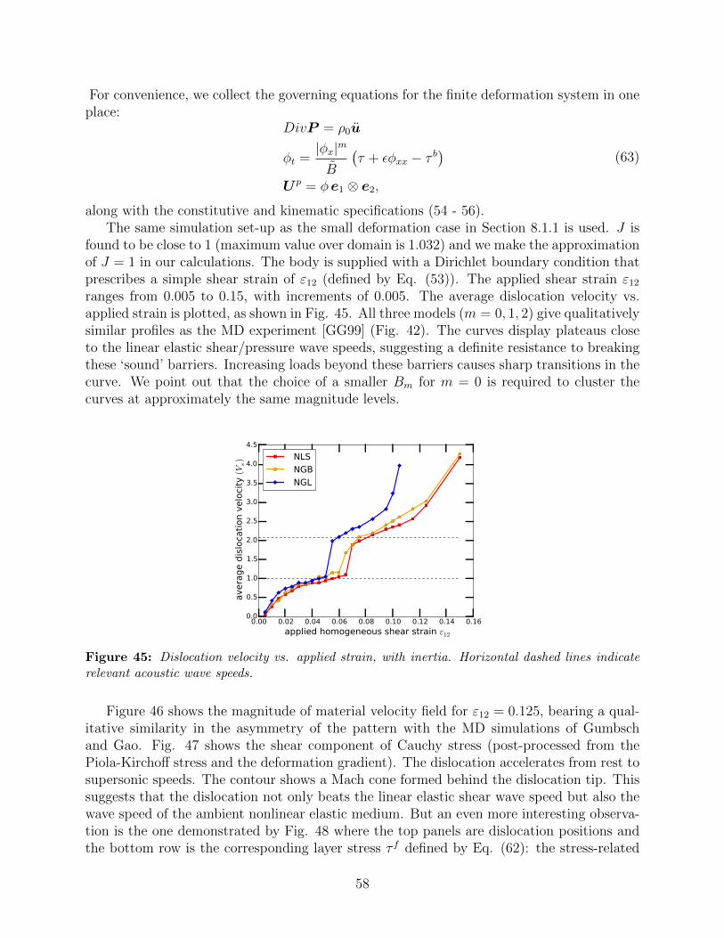
For convenience, we collect the governing equations for the finite deformation system in oneplace:

DivP = ρ0u

φt =|φx|m

B

(τ + εφxx − τ b

)U p = φ e1 ⊗ e2,

(63)

along with the constitutive and kinematic specifications (54 - 56).The same simulation set-up as the small deformation case in Section 8.1.1 is used. J is

found to be close to 1 (maximum value over domain is 1.032) and we make the approximationof J = 1 in our calculations. The body is supplied with a Dirichlet boundary condition thatprescribes a simple shear strain of ε12 (defined by Eq. (53)). The applied shear strain ε12

ranges from 0.005 to 0.15, with increments of 0.005. The average dislocation velocity vs.applied strain is plotted, as shown in Fig. 45. All three models (m = 0, 1, 2) give qualitativelysimilar profiles as the MD experiment [GG99] (Fig. 42). The curves display plateaus closeto the linear elastic shear/pressure wave speeds, suggesting a definite resistance to breakingthese ‘sound’ barriers. Increasing loads beyond these barriers causes sharp transitions in thecurve. We point out that the choice of a smaller Bm for m = 0 is required to cluster thecurves at approximately the same magnitude levels.

0.00 0.02 0.04 0.06 0.08 0.10 0.12 0.14 0.16

applied homogeneous shear strain ε12

0.0

0.5

1.0

1.5

2.0

2.5

3.0

3.5

4.0

4.5

avera

ge d

islo

cati

on v

elo

city

(Vs)

Vs

Vp

NLS

NGB

NGL

Figure 45: Dislocation velocity vs. applied strain, with inertia. Horizontal dashed lines indicaterelevant acoustic wave speeds.

Figure 46 shows the magnitude of material velocity field for ε12 = 0.125, bearing a qual-itative similarity in the asymmetry of the pattern with the MD simulations of Gumbschand Gao. Fig. 47 shows the shear component of Cauchy stress (post-processed from thePiola-Kirchoff stress and the deformation gradient). The dislocation accelerates from rest tosupersonic speeds. The contour shows a Mach cone formed behind the dislocation tip. Thissuggests that the dislocation not only beats the linear elastic shear wave speed but also thewave speed of the ambient nonlinear elastic medium. But an even more interesting observa-tion is the one demonstrated by Fig. 48 where the top panels are dislocation positions andthe bottom row is the corresponding layer stress τ f defined by Eq. (62): the stress-related

58

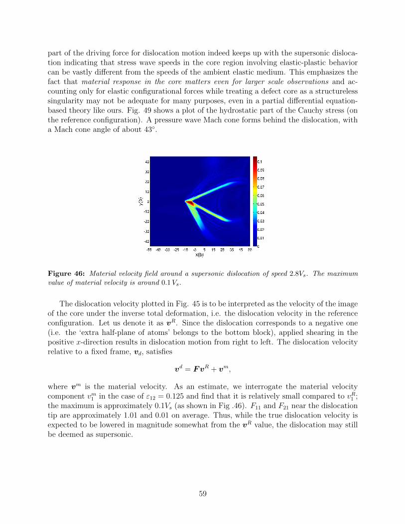
part of the driving force for dislocation motion indeed keeps up with the supersonic disloca-tion indicating that stress wave speeds in the core region involving elastic-plastic behaviorcan be vastly different from the speeds of the ambient elastic medium. This emphasizes thefact that material response in the core matters even for larger scale observations and ac-counting only for elastic configurational forces while treating a defect core as a structurelesssingularity may not be adequate for many purposes, even in a partial differential equation-based theory like ours. Fig. 49 shows a plot of the hydrostatic part of the Cauchy stress (onthe reference configuration). A pressure wave Mach cone forms behind the dislocation, witha Mach cone angle of about 43.

Figure 46: Material velocity field around a supersonic dislocation of speed 2.8Vs. The maximumvalue of material velocity is around 0.1Vs.

The dislocation velocity plotted in Fig. 45 is to be interpreted as the velocity of the imageof the core under the inverse total deformation, i.e. the dislocation velocity in the referenceconfiguration. Let us denote it as vR. Since the dislocation corresponds to a negative one(i.e. the ‘extra half-plane of atoms’ belongs to the bottom block), applied shearing in thepositive x-direction results in dislocation motion from right to left. The dislocation velocityrelative to a fixed frame, vd, satisfies

vd = FvR + vm,

where vm is the material velocity. As an estimate, we interrogate the material velocitycomponent vm1 in the case of ε12 = 0.125 and find that it is relatively small compared to vR1 ;the maximum is approximately 0.1Vs (as shown in Fig .46). F11 and F21 near the dislocationtip are approximately 1.01 and 0.01 on average. Thus, while the true dislocation velocity isexpected to be lowered in magnitude somewhat from the vR value, the dislocation may stillbe deemed as supersonic.

59

(a) (b) (c) (d)

Figure 47: From right to left, Cauchy stress wave (shear component) of a dislocation movingsupersonically under applied shear strain ε12 = 0.125. The arrows denote the positions of thedislocation core. From (d) to (c), as the dislocation is gaining speed to supersonic the region to theleft of the core is also accelerating, which generates disturbance around that area. The dislocationmoving with supersonic speed ((b) and (a)) forms behind the core a shear stress mach cones.

60 40 20 0 20 40 600.000.050.100.150.200.250.300.350.40

φx

60 40 20 0 20 40 60

x(b)

0.100.050.000.050.100.150.200.250.30

σ

(a)

60 40 20 0 20 40 600.000.050.100.150.200.250.300.350.400.45

φx

60 40 20 0 20 40 60

x(b)

0.100.050.000.050.100.150.200.250.30

σ

(b)

60 40 20 0 20 40 600.000.050.100.150.200.250.300.350.40

φx

60 40 20 0 20 40 60

x(b)

0.05

0.00

0.05

0.10

0.15

0.20

0.25

0.30

σ

(c)

60 40 20 0 20 40 600.0

0.1

0.2

0.3

0.4

0.5

φx

60 40 20 0 20 40 60

x(b)

0.15

0.20

0.25

0.30

0.35

0.40

σ

(d)

Figure 48: From right to left, the layer stress τ (bottom) moves with the dislocation(top). Wavesexcited by dislocation motion ripples backwards only (to the right).

(a) (b) (c) (d)

Figure 49: From right to left, hydrostatic part of Cauchy stress wave around the supersonicdislocation under applied shear strain ε12 = 0.125. The stable supersonic motion of the dislocationresults in a pressure wave mach cone forming behind the dislocation core.((b) and (a)).

It can be seen in the results of Fig. 47 and Fig. 49 that the Mach cone angles are obviouslydifferent between the top and the bottom blocks. In Fig. 47(b) as an example, the comparisonis approximately 32.9 (top) vs. 58.6 (bottom). Such asymmetry is not observed in thesmall deformation context (Fig. 44). We want to ascribe this asymmetry to the hypothesisthat the actual nonlinear wave speeds and propagation in the top and bottom blocks are

60

significantly different due to the differences in the elastic strain fields there. Compared tosmall deformation theory where the wave speeds are simply material properties, we arguethat in the calculations of Fig. 47, the stiffness largely depends on deformation states, whichaffects the wave speeds. The significant asymmetry between the top and bottom half bodyis well established, i.e., a negative edge dislocation results in a tensile stress in the horizontaldirection in the vicinity of the layer in the top block and a compressive stress field in thebottom block. In Table 6 we record Ee of two points vertically close to the dislocation(but outside the layer) for three arbitrary time steps during the supersonic motion of thedislocation. One can see that Ee

11 not only has opposite signs between the top and bottombut also different absolute values; other components do not show such large asymmetry.

The separated nature of the Mach cone wings in all cases is also worthy of note; to whatextent material heterogeneity (in the vertical direction) plays a role in this phenomenonremains to be explored.

Time instant (b/Vs) T1 = 12.3 T2 = 8.19 T3 = 6.66

strain state (top)

(0.130 0.0600.060 0.014

) (0.032 0.1210.121 0.030

) (0.030 0.1190.119 0.030

)strain state (bottom)

(−0.092 0.0630.063 0.023

) (−0.041 0.1010.101 0.023

) (−0.051 0.0920.092 0.018

)Table 6: Strain states sampled at the top and bottom of a supersonic dislocation at three timeinstants.

8.2 Longitudinal Shear band propagation modeled as dislocationmotion

Much like a crack-tip, a shear band is found to elongate through the motion of its tip[MD88, KW88, ZC03, GRR01]. Modeling this longitudinal extension of the band is a dif-ficult matter since classical plasticity theory does not provide a mechanism to achieve sucha dynamic extension mode, and delicate constitutive modifications have been resorted to[MLL07, ZRR96]. Here, we demonstrate this mode of shear band propagation as a directconsequence of dislocation motion, with the shear band tip interpreted as a dislocation linewith a nonsingular core. In Fig. 50 we plot the current configuration of the problem pre-sented previously in Fig. 47. The current coordinate of each node is simply a summationof the displacement and the reference coordinate. The motion of the dislocation leads tothe formation of a shear band between the point (10b, 0) and (50b, 0). We use a black arrowto indicate the position of the dislocation. The corresponding (total) deformation gradientcomponent F12 during the extension of the shear band is plotted in Fig. 51. The highlysheared region behind the dislocation is notable.

Interestingly, for shear bands formed in this way due to the motion of a localized curlof plastic deformation (the core), the shear band width is controlled by the geometry of thecore (here, its vertical extent) dragging the shear band behind it.

61

0 10 20 30 40 50 60

−10

−5

0

5

10

x(b)

y(b

)

0 10 20 30 40 50 60 70

−10

−5

0

5

10

x(b)

y(b

)

Figure 50: Shear band deformation formed behind the dislocation moving from (50b, 0) to (10b, 0).

(a) (b) (c) (d)

Figure 51: Deformation gradient F12 around shear band.

8.3 Effect of finite-speed-of-propagation of elastic waves

The time-dependent nature of the elastic fields of dislocations cannot be ignored especiallywhen modelling high strain rate processes. For situations involving ‘shock’ loadings andstrain rates higher than 106s−1, utilizing quasi-static dislocation stress fields is not appro-priate, even with an added mass correction to the equation of dislocation motion [HZL98].As a consequence, a new discrete dislocation approach was developed in [GLBD+13] to dealwith very high strain-rate deformations. In FDM, inertia is encoded in the system naturallythrough the balance law for linear momentum. The following example, directly adaptedfrom [GLBD+13], demonstrates the effect of finite-speed-of-propagation of elastic waves indislocation mechanics. The system is still governed by Eqs. (16) with m = 1 without anyfurther considerations of geometric or elastic nonlinearity.

A horizontal shock loading is applied on the left boundary by specifying the displacementat x = −55b as

u1(t) =

cos( πHy), t < 10

0, t >= 10.(64)

62

We insert a dislocation dipole in the center on the arrival of the shear stress front due to therapid boundary loading: a crude approximation to nucleating a dislocation. Fig. 52 showsthe series of shear stress contours during this process. Apart from the waves generated bythe shock loading, one can clearly see that it requires a finite time for stress waves due tothe dislocation dipole to propagate through the body. On the other hand, in a quasi-staticsetting, the elastic stress fields of the dipole would be transmitted all over the sample at theinstant the dipole is nucleated even with the added mass correction (since the issue is notrelated to the speed of the dislocation itself, but to the propagation of elastic fields).

(a) t = 50 bVs

(b) t = 275 bVs

(c) t = 350 bVs

(d) t = 450 bVs

Figure 52: Shear stress wave resulted by an artificially nucleated dislocation dipole.

To clearly demonstrate the finite-speed-of-propagation effect, we solve a quasi-staticdipole problem as in Section 7.1.6 for the displacement field us, and then superpose onus the dynamic displacement fields ud taken from Fig. 52(b) and evaluate the correspond-ing stress field (with φ also taken from Fig. 52(b)). Compared to the ‘quiet’ stress field infront of the loading pulse of Fig. 52(b), an instantaneous stress field of the nucleated dipoleis distributed immediately everywhere on the domain as nucleation occurs, shown in Fig.53. The magnitude of stress at the point (40b, 0) can reach up to 0.003µ while the value is2.8× 10−6µ at the same point in Fig. 52(b).

Figure 53: Quasi-static shear stress at the instant of the nucleated dislocation dipole.

63

8.4 Rupture Dynamics

In this section we explore the possibility of utilizing FDM in modeling aspects of dynamicrupture. As early as 1970, Brune [Bru70] suggested that an earthquake might be analogousto the problem of dislocation propagation in a slip plane. Nabarro [Nab87] mentions this aswell. At a very simplified level, rupture may be considered as the study of two very largeblocks of material slipping with respect to each other over a thin region (relative to the size ofthe blocks). Based on this picture, rupture dynamics has been primarily studied as a problemof friction between two bodies. A crack is assumed to exist behind the rupture front; thecrack faces are not traction free but transmit shear and normal stresses, the former limitedby a friction law. Very important for this conceptual picture is the fact that the relativedisplacement (slip) of the crack faces is not constitutively restricted, whereas the frictionlaw typically limits the maximum attainable shear stress that can be transmitted across therupture layer. For a general crack, any traction profile may be imposed on the crack surfacesas Neumann boundary conditions for the equations of elasticity, this being interpreted astwo conditions, one for each crack face. The friction law replaces these two conditions bydemanding traction continuity and constitutively relating the magnitude of the traction tothe displacement discontinuity across the layer.

On the other hand, for a classical dislocation in an elastic medium, there is again adisplacement discontinuity behind the dislocation line but of fixed magnitude, and the stressestransmitted across the dislocated part of the slip plane are not limited in principle, but haveto be continuous (except at the core singularity). A crack could in principle be loadedby Dirichlet boundary conditions, one for each face. The classical dislocation replaces thisspecified displacement boundary condition with a requirement of traction continuity anda specification of a displacement jump of fixed magnitude. An important fact about theclassical dislocation picture is that the material in the wake of the moving dislocation line isindistinguishable from the intact elastic material ahead of the dislocation, thus conferring anaspect of reversibility related to material response upon dislocation motion7. Moreover, theclassical notion of a dislocation and the substantial theory surrounding it related to solvingfor its fields allow no other possibility for material response behind the dislocation line. Itis physically clear, however, that this picture cannot then be applicable to the modelingof geophysical rupture as the phenomenon definitely requires some degradation in stressresponse behind the rupture front.

Against this backdrop, a primary aspect of rupture dynamics is the phenomenon ofself-healing. Self-healing is a conclusion deduced from observations of many earthquakerecords by Heaton [Hea90] which show that slip duration at any given point through whicha rupture front has propagated is relatively short compared to the duration of the wholeearthquake. Heaton also observed that it is a generic feature of crack models whose frictionlaws are of slip weakening type that short slip duration cannot be predicted. He furthersuggested [Hea90] slip velocity-weakening friction laws as a constitutive device that allows theaccommodation of the prediction of short-slip duration. This idea has since been developedin great quantitative detail, as explained in [Ric02]. On the other hand, were a rupturefront to be modeled as a dislocation line, it is a topological fact of the displacement fieldsof an isolated dislocation (i.e. a fixed Burgers vector) that only short slip duration can be a

7We thank Prof. J. R. Rice for emphasizing this fact.

64

consequence behind the rupture front.It seems to us that the dislocation picture and the crack picture are two extremes for

the modeling of rupture. The assumption that there is no elastic stiffness of material be-hind a rupture front, even though a fault zone is of non-negligible thickness and contains,presumably, pulverized material at great depths (and therefore compressive stress), seemsunrealistic to us. The shortcoming of the classical dislocation picture in dealing with thedamage behind the rupture front has already been mentioned. Thus, it seems that what maybe rather well-suited for the description of rupture is fundamentally a dislocation model thathowever allows for damage in elastic stiffness behind the rupture front. Field DislocationMechanics affords exactly this possibility and, as we show, interpolates between the crackand dislocation models depending on the extent of elastic damage allowed behind the rupturefront.

We modify the model described in Sec. 4 leading to the system (16) as follows. We modela fault zone as a layer with a modulus CL that is weaker than the outer region. We definethe damaged elasticity tensor in the layer as,

CL = (λ− φ

φκ)C, where 0 < κ < λ < 1. (65)

C is the undamaged elasticity tensor of the domain excluding the fault layer. When φ = 0,the non-ruptured layer has modulus λC, while ruptured portions of the fault have an evenweaker modulus (λ − κ)C. We keep all other features of the model as before. An implicitphysical assumption here is that in the absence of constraints due to compatibility of totaldeformations, the total strains exhibited by the material in the fault zone has preferredstrained states that can coexist. This is necessary. As shown before in Sec. 6.1, this isessential for a stress inducing feature as a rupture front to exist in equilibrium (as presumablyit does before its motion that triggers earthquakes). For the nonconvex function η (13), theexercise related to rupture modeling does not require a periodic potential and a triple wellpotential with wells at ±φ, 0 suffices.

For the purpose of illustration, we choose λ = 0.7 in this section, and κ is assumed totake the three values of 0.2, 0.6, 0.695. Therefore the elastic modulus of the undamaged fault(where φ = 0) is 0.7 of the outer blocks. The fault is assumed to be completely damagedwhere φ = φ and the damaged modulus is (0.7 − κ)C, i.e., a bigger κ represents greaterdamage. Within the core region the level of damage attains intermediate values as a functionof φ.

We start by studying the layer stress τ and slip δ (6) at a fixed observation point P inthe path of a moving dislocation/rupture front. Specifically, the dislocation is initialized atx = 0 and driven left by applying Dirichlet boundary condition, which prescribes a constantsimple shear deformation (defined by Eq. (53)). We utilize the NLS (m = 1) dynamics,for no particular reason. Fig. 54(a) shows τ and δ vs. time records at P : (−25b, 0) underan applied shear strain ε12 = 0.03 and κ = 0.2. Starting from an NLS dislocation pre-equilibrium, the dislocation is driven to the left by the applied strain and passes P at thetime t = 490 b/Vs. It is interesting to see that both quantities jump when the dislocationpasses through the observation point P . We note that the slip stabilizes at a point once thedislocation passes through. This slip field is simply the sum of the (layer-integrated) elasticand plastic distortions at each point in the layer. The kinematics of dislocation motion

65

encoded in FDM ensures that there is no evolution of plastic distortion at a point once theentire core has traversed through it, due to the absence of plastic distortion gradients behindthe dislocation core.

0 100 200 300 400 500 600 700 800 900 Time (b/Vs )

0.0

0.1

0.2

0.3

0.4

0.5

0.6

δ(b)

0.02

0.00

0.02

0.04

0.06

0.08

0.10

0.12

0.14

τ(µ)

(a) τ and δ

0 1 2 3 4 50.6

0.5

0.4

0.3

0.2

0.1

0.0

0.1

Parkfield sketch

0 100 200 300 400 500 Time(b/Vs)

0.14

0.12

0.10

0.08

0.06

0.04

0.02

0.00

FDM

(b) u2

Figure 54: Left: layer stress and slip calculated at a fixed point (x = −25b) in the passage of arupture front. Right: transverse displacement at a fixed point in the rupture passage calculated byFDM model compared with sketch of the observed data recorded in the Parkfield earthquake. Sketchadapted from [AR02] (Copyright University Science Books, used with permission).

0 100 200 300 400 500 600 700 800 900 Time(b/Vs )

0.02

0.00

0.02

0.04

0.06

0.08

0.10

0.12

0.14

0.16

τ(µ

)

=0.695

=0.6

=0.2

(a) τ at x = −25b

0 100 200 300 400 500 600 700 800 900 Time(b/Vs )

0.0

0.2

0.4

0.6

0.8

1.0

1.2

1.4

1.6

δ(b

)

=0.695

=0.6

=0.2

0.067√t−326 +0.1

(b) δ at x = −25b

Figure 55: Layer stress(left) and slip(right) plotted at a fixed point on rupture front passage withvarying elasticity damage. κ = 0.695 is fit by a square root function.

Fig. 54(b) shows the transverse displacement fields recorded at the same point in thecase of κ = 0.2. The profile qualitatively agrees with the observed form from the Parkfieldearthquake sketched on the top [AR02].

Fig. 55(a) demonstrates how κ affects the layer stress behind the rupture front. Theconclusion is that the greater the ‘elastic damage’ behind the rupture front, the less is the

66

propensity of the stress to recover after the passage of the rupture front. Fig. 55(b) showsthe corresponding slip records. Note that the most damaged case (κ = 0.695) leads to amodel behavior similar to a crack model, i.e., the slip at any point in the ruptured zone keepsincreasing behind the rupture front as a square root function of time (unless rupture frontpropagation is forcibly stopped) - this is generically characteristic of all crack-like modelsof rupture dynamics employing slip-weakening friction laws [Hea90, DDLL05]. At the veryleast, then, FDM-based modeling of rupture dynamics appears to recover the response totwo vastly different frictional constitutive assumptions via a simple assumption of damageof elastic modulus.

The following observations related to our preliminary foray into the modeling of ruptureare in order:

• FDM naturally allows for the addition of a model of plastic deformation in the wakeof the dislocation reflecting plastic straining in the absence of its spatial variation, asin classical plasticity theory. In fact, such a mode of plastic deformation is regularlyused in applications of FDM at larger length scales [RA06, PDA11, FAB11]. In cir-cumstances when the elastic modulus is substantially degraded behind the dislocationfront, such an augmentation can accommodate the great variety of frictional consti-tutive assumptions (i.e. slip weakening, velocity weakening, rate-and-state friction)utilized in the current modeling of rupture dynamics. In ongoing work in simplifiedmodels, such a combination has been observed to give rise to stick-slip behavior.

• Due to the dependence of the elastic modulus on the plastic strain, the driving force forthe dislocation (rupture front) velocity should contain a term arising from ∂φC thatwe have ignored for simplicity. This term is expected to affect the observed velocity ofthe rupture front and not the conclusions related to the existence of short slip durationor the lack of it.

• Modeling thick faults with substantial field variations through the thickness is appar-ently an important issue in realistic modeling of rupture [RC07]. We note that FDM isa full 3-dimensional theory and can be invoked within the fault layer with no conceptualdifficulty.

• Slow rupture fronts [RCF04, CAS99] are observed. As mentioned earlier, there isa parameter regime (i.e. large drag) for our theory where such phenomena can bemodeled.

• For the sake of simplicity, we have not introduced a normal-stress dependence in rup-ture propagation. We note that even the simplified model of FDM utilized in thispaper allows naturally for the emergence of a normal-stress dependence in the rupturevelocity, as shown in the development of Section 4.

9 Concluding Remarks

It is perhaps fair to say that at the current time the classical theory of dislocations [HL82]and the theory of elastoplasticity [Lub01] appear to be disparate subjects. We hope to have

67

demonstrated in this paper that FDM, which is nothing but a theory of elastoplasticity witha fancy, but physically rigorous, evolution equation for the plastic distortion, encompassesa large class of key features of classical dislocation theory in both its extensively developedstatic and its barely developed time-dependent aspects. This observation is particularlyimportant in situations involving dynamics with inertia where the classical theory has severeconceptual limitations.

The computational methods of approximation that we use to study FDM are versatileand capable of natural extension to 3 space dimensions, representation of multiple slip, finitedeformations (in full generality), elastic anisotropy, arbitrary loadings, and complex domains.This is desirable, both from the scientific and engineering points of view. In a sense, thetheory and methods we propose for the study of dislocation mechanics have the potential ofbringing the same type of efficiency and generality to the study of the physical subject asthe finite element method did to the study of elasticity theory. Indeed, a reading of paperslike that of Eshelby, Frank, and Nabarro [EFN51] leaves one marveling at the creativity ofthe authors; however, the techniques utilized are very special. Our approximation methodsare accessible to anyone with training in the standard repertoire of computational mechanicswith a desire to learn about dislocation mechanics, and this is as much a result of thetheoretical framework that is employed.

Starting from the pioneering work of Aifantis [Aif84] there has been a great emphasis inthe solid mechanics community in developing models of strain gradient plasticity in the last30 years or so, often to make connection with dislocation mechanics. It is again perhaps fairto say that while many models have emerged, none can lay claim to being a theory for themechanics of dislocations in any distinguished limit, whether for individual or collective be-havior. In contrast, we have shown that the equations of FDM, which may also be consideredas a gradient-plasticity model in the form (5), but of very different structure compared tobona-fide standard strain gradient plasticity theories, can make the claim at the level of rep-resenting a great variety of individual dislocation behavior. There are important questionsof time-dependent homogenization related to the modeling of mesoscopic and macroscopicplasticity that remain to be addressed, but we take satisfaction in the fact that a correctpde-based microscopic standpoint has been established. Moreover, work based on heuris-tic models of collective behavior developed on FDM as the underlying microscopic theoryhas shown promise [AR06, RA06, PDA11, ABM08, FAB11, CCP+13], including the demon-stration of how standard elastoplasticity theory can be incorporated within the theoreticalstructure if so desired.

The most important future work related to FDM that remains for us to execute is arobust computational implementation of the 3-d theory without restriction to special ‘sliplayers,’ with slip-system like behavior being an outcome. This will require careful design ofthe energetics related to slip (i.e. the η function) and, very importantly, an accurate andstable numerical scheme for the U p evolution equation which will need to be capable of rep-resenting dynamic, string-like, nonsingular, stress-inducing localizations in the field. Despiteappearances arising from the simplified ansatz we have utilized in this paper, the funda-mental 3-d equations of FDM are not a variation on reaction diffusion systems or scalar,hyperbolic, conservation laws; see [AT11] for illustration of this issue. These are interesting,but tractable, challenges. The question related to energetics also has an important philo-sophical angle in that it should be defined purely in terms of quantities identifiable from the

68

current state without reference to any reference configuration in the past, and the plasticdistortion does not readily lend itself to such definition. It is very likely that resolution willlie in a careful adaptation of ideas from [RBS92, Vit68, SW03, Zim04, Par10, NP14].

Acknowledgment

This research was supported in part by the National Science Foundation through grant CMMI1435624. Generous grants of computer time and help from Pittsburgh SupercomputingInstitute are gratefully acknowledged.

References

[ABM08] Amit Acharya, Armand Beaudoin, and Ron Miller. New perspectives in plas-ticity theory: dislocation nucleation, waves, and partial continuity of plasticstrain rate. Mathematics and Mechanics of Solids, 13(3-4):292–315, 2008.

[Ach01] Amit Acharya. A model of crystal plasticity based on the theory of continu-ously distributed dislocations. Journal of the Mechanics and Physics of Solids,49(4):761–784, 2001.

[Ach03] Amit Acharya. Driving forces and boundary conditions in continuum disloca-tion mechanics. Proceedings of the Royal Society of London. Series A: Mathe-matical, Physical and Engineering Sciences, 459(2034):1343–1363, 2003.

[Ach04] Amit Acharya. Constitutive analysis of finite deformation field dislocationmechanics. Journal of the Mechanics and Physics of Solids, 52(2):301–316,2004.

[Ach07] Amit Acharya. Jump condition for GND evolution as a constraint on sliptransmission at grain boundaries. Philosophical magazine, 87(8-9):1349–1359,2007.

[Ach10] Amit Acharya. New inroads in an old subject: plasticity, from around theatomic to the macroscopic scale. Journal of the Mechanics and Physics ofSolids, 58(5):766–778, 2010.

[Ach11] Amit Acharya. Microcanonical entropy and mesoscale dislocation mechanicsand plasticity. Journal of Elasticity, 104(1-2):23–44, 2011.

[AHLBM06] Olivier Alvarez, Philippe Hoch, Yann Le Bouar, and Regis Monneau. Dislo-cation dynamics: short-time existence and uniqueness of the solution. Archivefor Rational Mechanics and Analysis, 181(3):449–504, 2006.

[Aif84] E. C. Aifantis. On the microstructural origin of certain inelastic models. Journalof Engineering Materials and Technology, 106(4):326–330, 1984.

69

[AMZ10] Amit Acharya, Karsten Matthies, and Johannes Zimmer. Travelling wave so-lutions for a quasilinear model of field dislocation mechanics. Journal of theMechanics and Physics of Solids, 58(12):2043–2053, 2010.

[AR02] Keiiti Aki and Paul G. Richards. Quantitative Seismology. University ScienceBooks, 2002.

[AR06] Amit Acharya and Anish Roy. Size effects and idealized dislocation microstruc-ture at small scales: predictions of a phenomenological model of mesoscopicfield dislocation mechanics: Part I. Journal of the Mechanics and Physics ofSolids, 54(8):1687–1710, 2006.

[AT11] Amit Acharya and Luc Tartar. On an equation from the theory of field dislo-cation mechanics. Bollettino dell’ Unione Matematica Italiana, 9(IV):409–444,2011.

[AZ14] Amit Acharya and Xiaohan Zhang. From dislocation motion to an additive ve-locity gradient decomposition, and some simple models of dislocation dynam-ics. In Ta-Tsien Li and Ph. G. Ciarlet, editors, Proceedings of the InternationalConference in honor of Luc Tartar on Nonlinear and Multiscale Partial Differ-ential Equations: Theory, Numerics and Applications; Series in ContemporaryApplied Mathematics. Higher Education Press (Beijing) and World Scientific,Singapore, 2014.

[BCBK06] V. V. Bulatov, W. Cai, R. Baran, and K. Kang. Geometric aspects of theideal shear resistance in simple crystal lattices. Philosophical Magazine, 86(25-26):3847–3859, 2006.

[BJC+01] V.V. Bulatov, J.F. Justo, Wei Cai, Sidney Yip, A.S. Argon, T. Lenosky, M. deKoning, and T. Diaz de la Rubia. Parameter-free modelling of dislocationmotion: the case of silicon. Philosophical Magazine A, 81(5):1257–1281, 2001.

[Bru70] James N. Brune. Tectonic stress and the spectra of seismic shear waves fromearthquakes. Journal of Geophysical Research, 75(26):4997–5009, 1970.

[CAS99] Luca Crescentini, Antonella Amoruso, and Roberto Scarpa. Constraints on slowearthquake dynamics from a swarm in central Italy. Science, 286(5447):2132–2134, 1999.

[CAWB06] Wei Cai, Athanasios Arsenlis, Christopher R. Weinberger, and Vasily V. Bula-tov. A non-singular continuum theory of dislocations. Journal of the Mechanicsand Physics of Solids, 54(3):561–587, 2006.

[CCHO97] A. Carpio, S. J. Chapman, S. D. Howison, and J. R. Ockendon. Dynamics ofline singularities. Philosophical Transactions of the Royal Society of London.Series A: Mathematical, Physical and Engineering Sciences, 355(1731):2013–2024, 1997.

70

[CCP+13] Yong S. Chen, Woosong Choi, Stefanos Papanikolaou, Matthew Bierbaum, andJames P. Sethna. Scaling theory of continuum dislocation dynamics in threedimensions: Self-organized fractal pattern formation. International Journal ofPlasticity, 46:94–129, 2013.

[CCV01] Ana Carpio, S. Jonathan Chapman, and J. J. L. Velazquez. Pile-up solutions forsome systems of conservation laws modelling dislocation interaction in crystals.SIAM Journal on Applied Mathematics, 61(6):2168–2199, 2001.

[CP89] Jack Carr and Robert L. Pego. Metastable patterns in solutions of ut = ε2uxx−f(u). Communications on Pure and Applied Mathematics, 42(5):523–576, 1989.

[DAZM13] Amit Das, Amit Acharya, Johannes Zimmer, and Karsten Matthies. Can equa-tions of equilibrium predict all physical equilibria? A case study from Field Dis-location Mechanics. Mathematics and Mechanics of Solids, 18:801–820, 2013.

[DDLL05] Steven M. Day, Luis A. Dalguer, Nadia Lapusta, and Yi Liu. Comparisonof finite difference and boundary integral solutions to three-dimensional spon-taneous rupture. Journal of Geophysical Research: Solid Earth (1978–2012),110(B12), 2005.

[Den04] Christophe Denoual. Dynamic dislocation modeling by combining PeierlsNabarro and Galerkin methods. Physical Review B, 70(2):024106, 2004.

[EFN51] J.D. Eshelby, F.C. Frank, and F.R.N. Nabarro. The equilibrium of linear arraysof dislocations. Philosophical Magazine, 42(327):351–364, 1951.

[FAB11] C. Fressengeas, A. Acharya, and A. J. Beaudoin. Dislocation mediated contin-uum plasticity: Case studies on modeling scale dependence, scale-invariance,and directionality of sharp yield-point. In S. Ghosh and D. M. Dimiduk, editors,Computational Methods for Microstructure-Property Relationships. Springer,2011.

[Fox66] N. Fox. A continuum theory of dislocations for single crystals. IMA Journal ofApplied Mathematics, 2(4):285–298, 1966.

[Fre98] L. B. Freund. Dynamic fracture mechanics. Cambridge University Press, 1998.

[GAM15] Akanksha Garg, Amit Acharya, and Craig E. Maloney. A study of conditionsfor dislocation nucleation in coarser-than-atomistic scale models. Journal ofthe Mechanics and Physics of Solids, 75:76–92, 2015.

[GG99] Peter Gumbsch and Huajian Gao. Dislocations faster than the speed of sound.Science, 283(5404):965–968, 1999.

[GLBD+13] Benat Gurrutxaga-Lerma, Daniel S. Balint, Daniele Dini, Daniel E. Eakins,and Adrian P. Sutton. A dynamic discrete dislocation plasticity method forthe simulation of plastic relaxation under shock loading. Proceedings of theRoyal Society A: Mathematical, Physical and Engineering Science, 469(2156),2013.

71

[GRR01] P. R. Guduru, A. J. Rosakis, and G. Ravichandran. Dynamic shear bands: aninvestigation using high speed optical and infrared diagnostics. Mechanics ofMaterials, 33(7):371–402, 2001.

[Hea90] Thomas H. Heaton. Evidence for and implications of self-healing pulses of slipin earthquake rupture. Physics of the Earth and Planetary Interiors, 64(1):1–20, 1990.

[HL82] John P. Hirth and Jens Lothe. Theory of dislocations. John Wiley & Sons,1982.

[HZL98] J.P. Hirth, H.M. Zbib, and J. Lothe. Forces on high velocity dislocations.Modelling and Simulation in Materials Science and Engineering, 6(2):165, 1998.

[IRG15] Mrinal Iyer, Balachandran Radhakrishnan, and Vikram Gavini. Electronic-structure study of an edge dislocation in aluminum and the role of macroscopicdeformations on its energetics. Journal of the Mechanics and Physics of Solids,76:260–275, 2015.

[KBC12] Keonwook Kang, Vasily V. Bulatov, and Wei Cai. Singular orientations andfaceted motion of dislocations in body-centered cubic crystals. Proceedings ofthe National Academy of Sciences, 109(38):15174–15178, 2012.

[KCC+92] Ladislas P. Kubin, G. Canova, M. Condat, Benoit Devincre, V. Pontikis, andYves Brechet. Dislocation microstructures and plastic flow: a 3d simulation.Solid State Phenomena, 23:455–472, 1992.

[KCO02] Marisol Koslowski, Alberto M. Cuitino, and Michael Ortiz. A phase-field the-ory of dislocation dynamics, strain hardening and hysteresis in ductile singlecrystals. Journal of the Mechanics and Physics of Solids, 50(12):2597–2635,2002.

[Kro81] Ekkehart Kroner. Continuum theory of defects. In R. Balian and M. Klemanet al., editors, Physics of Defects, Les-Houches Summer School, pages 217–315.North-Holland, Amsterdam, 1981.

[KW88] J. F. Kalthoff and S. Winkler. Failure mode transitions at high rates of loading.In L. W. Meyer C. Y. Chiem, H. D. Kunze, editor, Proceedings of the Inter-national Conference on Impact Loading and Dynamic Behavior of Materials,pages 43–56. DeutscheGesselschaft fur Metallkunde, 1988.

[LH59] J. Lothe and J.P. Hirth. Dislocation dynamics at low temperatures. PhysicalReview, 115(3):543, 1959.

[LKBK00] Gang Lu, Nicholas Kioussis, Vasily V. Bulatov, and Efthimios Kaxiras. ThePeierls-Nabarro model revisited. Philosophical Magazine Letters, 80(10):675–682, 2000.

72

[LS08] Surachate Limkumnerd and James P. Sethna. Shocks and slip systems: Pre-dictions from a mesoscale theory of continuum dislocation dynamics. Journalof the Mechanics and Physics of Solids, 56(4):1450–1459, 2008.

[Lub01] Vlado A. Lubarda. Elastoplasticity theory. CRC press, 2001.

[Mar11] Xanthippi Markenscoff. Comment on dynamic Peierls-Nabarro equations forelastically isotropic crystals. Physical Review B, 83(5):056101, 2011.

[MBW98] A. B. Movchan, R. Bullough, and J. R. Willis. Stability of a dislocation: discretemodel. European Journal of Applied Mathematics, 9(04):373–396, 1998.

[MD88] A. Marchand and J. Duffy. An experimental study of the formation processof adiabatic shear bands in a structural steel. Journal of the Mechanics andPhysics of Solids, 36(3):251–283, 1988.

[MLL07] Sergey N. Medyanik, Wing Kam Liu, and Shaofan Li. On criteria for dynamicadiabatic shear band propagation. Journal of the Mechanics and Physics ofSolids, 55(7):1439–1461, 2007.

[MPBO98] Ron Miller, Rob Phillips, Glen Beltz, and Michael Ortiz. A non-local formula-tion of the Peierls dislocation model. Journal of the Mechanics and Physics ofSolids, 46(10):1845–1867, 1998.

[Mur63] T. Mura. Continuous distribution of moving dislocations. Philosophical Mag-azine, 8(89):843–857, 1963.

[Nab47] F.R.N. Nabarro. Dislocations in a simple cubic lattice. Proceedings of thePhysical Society, 59(2):256, 1947.

[Nab87] F. R. N. Nabarro. Theory of crystal dislocations. Dover, 1987.

[NP14] Rachel Nicks and Gareth Parry. Group elastic symmetries common to con-tinuum and discrete defective crystals. Journal of Elasticity, 115(2):131–156,2014.

[Par10] Gareth P. Parry. Elastic symmetries of defective crystals. Journal of Elasticity,101(1):101–120, 2010.

[PDA11] Saurabh Puri, Amit Das, and Amit Acharya. Mechanical response of mul-ticrystalline thin films in mesoscale field dislocation mechanics. Journal of theMechanics and Physics of Solids, 59(11):2400–2417, 2011.

[PDT10] Y-P Pellegrini, Christophe Denoual, and Lev Truskinovsky. Phase-field model-ing of nonlinear material behavior. In IUTAM symposium on variational con-cepts with applications to the mechanics of materials, pages 209–220. Springer,2010.

[Pei40] R. Peierls. The size of a dislocation. Proceedings of the Physical Society,52(1):34–37, 1940.

73

[Pel10] Yves-Patrick Pellegrini. Dynamic Peierls-Nabarro equations for elasticallyisotropic crystals. Physical Review B, 81(2):024101, 2010.

[Pel11] Yves-Patrick Pellegrini. Reply to comment on dynamic Peierls-Nabarro equa-tions for elastically isotropic crystals. Physical Review B, 83(5):056102, 2011.

[Pic02] R.C. Picu. The Peierls stress in non-local elasticity. Journal of the Mechanicsand Physics of Solids, 50(4):717–735, 2002.

[PLSG14] Giacomo Po, Markus Lazar, Dariush Seif, and Nasr Ghoniem. Singularity-freedislocation dynamics with strain gradient elasticity. Journal of the Mechanicsand Physics of Solids, 68:161–178, 2014.

[RA06] Anish Roy and Amit Acharya. Size effects and idealized dislocation microstruc-ture at small scales: predictions of a phenomenological model of mesoscopicfield dislocation mechanics: Part II. Journal of the Mechanics and Physics ofSolids, 54(8):1711–1743, 2006.

[RBS92] J. R. Rice, G. E. Beltz, and Y. Sun. Peierls framework for dislocation nucleationfrom a crack tip. In Topics in fracture and fatigue, pages 1–58. Springer, 1992.

[RC07] James R. Rice and Massimo Cocco. Seismic fault rheology and earthquakedynamics. Tectonic Faults: Agents of Change on a Dynamic Earth, pages 99–137, 2007.

[RCF04] Shmuel M. Rubinstein, Gil Cohen, and Jay Fineberg. Detachment fronts andthe onset of dynamic friction. Nature, 430(7003):1005–1009, 2004.

[Ric71] James R. Rice. Inelastic constitutive relations for solids: an internal-variabletheory and its application to metal plasticity. Journal of the Mechanics andPhysics of Solids, 19(6):433–455, 1971.

[Ric02] James R. Rice. New perspectives on crack and fault dynamics. In Mechanicsfor a New Mellennium, pages 1–24. Springer, 2002.

[RLBF03] D. Rodney, Y. Le Bouar, and A. Finel. Phase field methods and dislocations.Acta Materialia, 51(1):17–30, 2003.

[RSC99] A.J. Rosakis, O. Samudrala, and D. Coker. Cracks faster than the shear wavespeed. Science, 284(5418):1337–1340, 1999.

[Sch99] G. Schoeck. Peierls energy of dislocations: a critical assessment. PhysicalReview Letters, 82(11):2310, 1999.

[SW03] C. Shen and Y. Wang. Phase field model of dislocation networks. Acta mate-rialia, 51(9):2595–2610, 2003.

[VBAF06] S. N. Varadhan, A. J. Beaudoin, A. Acharya, and C. Fressengeas. Dislocationtransport using an explicit Galerkin/Least-squares formulation. Modelling andSimulation in Materials Science and Engineering, 14(7):1245, 2006.

74

[Vit68] V. Vitek. Intrinsic stacking faults in body-centred cubic crystals. PhilosophicalMagazine, 18(154):773–786, 1968.

[WH74] W. W. Wood and A. K. Head. The motion of dislocations. Proceed-ings of the Royal Society of London. A. Mathematical and Physical Sciences,336(1605):191–209, 1974.

[Wil65] J. R. Willis. Dislocations and inclusions. Journal of the Mechanics and Physicsof Solids, 13(6):377–395, 1965.

[Wil67] John R. Willis. Second-order effects of dislocations in anisotropic crystals.International Journal of Engineering Science, 5(2):171–190, 1967.

[WJCK01] Yu U. Wang, Y. M. Jin, A. M. Cuitino, and A. G. Khachaturyan. Nanoscalephase field microelasticity theory of dislocations: model and 3d simulations.Acta Materialia, 49(10):1847–1857, 2001.

[WL10] Yunzhi Wang and Ju Li. Phase field modeling of defects and deformation. ActaMaterialia, 58(4):1212–1235, 2010.

[XCSE03] Yang Xiang, Li-Tien Cheng, David J. Srolovitz, and Weinan E. A level setmethod for dislocation dynamics. Acta Materialia, 51(18):5499–5518, 2003.

[ZC03] Z. Zhang and R. J. Clifton. Shear band propagation from a crack tip. Journalof the Mechanics and Physics of Solids, 51(11):1903–1922, 2003.

[Zim04] Johannes Zimmer. Stored energy functions for phase transitions in crystals.Archive for Rational Mechanics and Analysis, 172(2):191–212, 2004.

[ZRR96] M. Zhou, G. Ravichandran, and A.J. Rosakis. Dynamically propagating shearbands in impact-loaded prenotched plates – II. numerical simulations. Journalof the Mechanics and Physics of Solids, 44(6):1007–1032, 1996.

75