a single-camera method for three-dimensional video imaging

A single-camera method for three-dimensional video imaging

J. Eian a,b,*, R.E. Poppele a

a Department of Neuroscience, 321 Church Street, SE, University of Minnesota, Minneapolis, MN 55455, USAb Graduate Program in Biomedical Engineering, University of Minnesota, Minneapolis, MN 55455, USA

Received 22 March 2001; received in revised form 27 June 2002; accepted 28 June 2002

Abstract

We describe a novel method for recovering the three-dimensional (3D) point geometry of an object from images acquired with a

single-camera. Typically, multiple cameras are used to record 3D geometry. Occasionally, however, there is a need to record 3D

geometry when the use of multiple cameras is either too costly or impractical. The algorithm described here uses single-camera

images and requires in addition that each marker on the object be linked to at least one other marker by a known distance. The

linkage distances are used to recover information about the third dimension that would otherwise be lost in single-camera two-

dimensional images. The utilities of the method are its low-cost, simplicity, and ease of calibration and implementation. We were

able to estimate 3D distances and positions as accurately as with a commercially available multi-camera 3D system. This method

may be useful in pilot studies to determine whether 3D imaging systems are required, or, it can serve as a low-cost alternative to

multi-camera systems. # 2002 Elsevier Science B.V. All rights reserved.

Keywords: Reconstruction; Three-dimension; Video; Kinematics; Biomechanics; Gait

1. Introduction

Video imaging is often used to record the three-

dimensional (3D) geometry of objects in space. A

number of different methods exist, and most make use

of images acquired with multiple cameras (see Shapiro,

1980 for a review). The direct linear transformation

method (Abdel-Aziz and Karara, 1971) is a widely used

technique because it is accurate and relatively simple to

implement (Yu et al., 1993). It requires images from at

least two cameras for 3D reconstruction.

Occasionally, however, the use of multiple cameras is

either impractical or too costly. A number of single-

camera methods exist, but most record just two-dimen-

sional (2D) geometry (Smith and Fewster, 1995). Only a

handful of single-camera methods for 3D data collection

have been described, and each imposes the need for

something in addition to the camera images. Berstein

(1930) (see also Shapiro, 1980) described a single-camera

3D application that used a mirror to provide a second

view of the object so multi-image techniques could be

applied to a single split image. Positioning the mirror is

an evident drawback of this approach.

Miller et al. (1980) described another single-camera

3D method that does not require multiple views of the

object. It is an extension of a multi-camera 3D

cinematographic method that applies to objects coupled

by joints with known characteristics; knowledge of the

joint characteristics allows 3D information to be ex-

tracted from 2D images. We propose here a somewhat

similar single-camera 3D approach that also makes use

of specific knowledge about object geometry.

Indeed, it is impossible to determine the 3D position

of a lone marker in space from 2D images acquired with

one stationary camera, and the method proposed here

cannot be used for such a task. It can, however, be used

to determine the positions of multiple markers in space

when each marker is linked to at least one other marker

by a known distance. The linkage distances are used to

recover information about the third dimension that

would otherwise be acquired with a second camera.

Numerous objects possess the geometry required for this

approach; for example, joint markers on a limb suffice

because the lengths of the bones that span the joints

provide the required linkage distances.

* Corresponding author. Tel.: �/1-612-625-4412; fax: �/1-612-626-

5009

E-mail address: [email protected] (J. Eian).

Journal of Neuroscience Methods 120 (2002) 65�/83

www.elsevier.com/locate/jneumeth

0165-0270/02/$ - see front matter # 2002 Elsevier Science B.V. All rights reserved.

PII: S 0 1 6 5 - 0 2 7 0 ( 0 2 ) 0 0 1 9 1 - 7

mailto:[email protected]

The utility of the method is its relative simplicity and

low-cost. The only required equipment is one camera

and a system capable of locating image points in a 2D

plane. No measurements of camera position or orienta-tion are needed, and the required calibration is simple: it

amounts to recording still images of a marker grid

moved incrementally through the depth of the object

workspace.

Reconstruction accuracy depends primarily on the

care taken in performing the calibration and the

accuracy of the imaging system. In the study described

here we were able to estimate 3D lengths and positionsas accurately as with a commercially available multi-

camera 3D system*/with a marked reduction in system

complexity and cost. This method seems well suited for

pilot studies to determine whether a standard single-

camera 2D system or a more expensive multi-camera 3D

system is needed. It may also serve as a simple low-cost

alternative when the imaged objects meet the linkage

requirement.

2. Theoretical overview

2.1. Example

In order to see how distance information can be used

to reconstruct 3D geometry from a single 2D image, we

begin by discussing a two-point example. Consider apoint O arbitrarily positioned in space, and a second

point, P , linked to O by a known distance, D. We can

determine the position of P relative to O using D and an

image of this geometry. The image contains two points,

call them o and p , generated by O and P , respectively

(Fig. 1). The location of p in the image specifies the

camera line of sight that must contain P . The problem

of locating P in 3D space amounts to determining whereP lies along this line of sight. We can narrow this down

to two possible positions by visualizing a spherical shell

with radius D centered O . The shell represents all

possible positions of P relative to O . The line of sight

specified by p can intersect this shell at most twice (P1

and P2), and these two intersections are the only

possible positions of P relative to O given the image

data. We can remove the final ambiguity by consideringeither known characteristics of the geometry (for

example, of an object represented by the points), or,

more generally, a third point linked to P . In the latter

case, the distance from P to the third point will usually

be satisfied by only one of positions P1 and P2 (we

explain this further below and the appendices).

We have devised a tractable mathematical algorithm

to determine 3D information in a manner analogous tothis example. The algorithm requires a calibration that

allows us to assign a camera line of sight to each

location in the image. Each line of sight is the ray that

contains all points in space that appear at a particular

location in the image. The use of rays allows us to

express all three unknown coordinates of an image

producing point in terms of a single unknown coordi-

nate. The specification is provided by equations derived

from the calibration.

The way we use this coordinate reducing property of

the rays in the algorithm can be illustrated with our

example. Analogous to the shell about O , we use a 3D

Euclidean distance formula to express the distance

between O and P in terms of their three unknown

coordinates. Next we turn to the image. It contains

points o and p , and their locations specify rays that

contain points O and P , respectively. Using equations

that model these rays, we express all three unknown

coordinates of O and P in terms of one unknown

coordinate for each point. By substituting these equa-

tions into the distance formula we reduce it to an

equation with only two unknowns: one coordinate for O

and one coordinate for P . If we know the coordinate for

one point, O for example, we can solve for the

coordinate of the other.

Thus the algorithm requires, in addition to the known

distances between markers, one spatial coordinate of a

seeding marker. We can work iteratively and determine

the 3D positions of all the markers linked to the seeding

marker through chains of known distances. There are at

least two ways to determine a coordinate for a seeding

marker. The first is to know one coordinate of a marker

beforehand. For example, we moved objects with a

robot, so from knowledge of the robot path we knew a

Fig. 1. Algorithm geometry: Given two points in space, O and P , and

the distance between them, D, all possible positions of P relative to O

are represented by an invisible spherical shell centered at O with radius

D. A focused image of the points eliminates all but two possible

positions for P . The image contains two points, o and p , generated by

O and P , respectively. Point p in the image specifies the line of sight

that must contain P in space, and this line of sight can intersect the

shell about O at no more than two points, P1 and P2. These are the

only possible positions of P relative to O given the image. This is the

basis of the reconstruction algorithm. We develop a mathematical

model of this geometry in the text.

J. Eian, R.E. Poppele / Journal of Neuroscience Methods 120 (2002) 65�/8366

coordinate for a marker affixed to the robot. Given the

known coordinate, the equations for the ray that

contains the marker specify the other two coordinates.

There is also a second way that can be used if nocoordinate of any marker is known. It requires a triangle

of distances between three markers and an image of the

markers. We describe it in Appendix C.

2.2. Preliminary description and definitions

Here we define the terminology used in the mathe-

matical derivations that follow. We call what we are

imaging the object or subject . We select a finite set ofpoints on the object to describe its geometry, and we call

these points markers . When the distance between two

markers on the object is known we say the markers are

linked . We use markers and their images to represent the

geometry of the object in three domains (to be defined):

3D space, the 2D image plane, and the 2D video frame.

3D space , or simply space , is the field of view of the

camera. We assume that the object is always in 3Dspace. We allow any three orthogonal directions, X , Y ,

and Z , to be selected as a basis for 3D space, but in the

descriptions that follow we assumed X�horizontal,

Y�vertical, and Z�depth, where in this case � means

‘is most nearly parallel to’ and depth is along the optical

axis of the camera. The units of length in space are (cm).

We denote O to be the origin in 3D space and the

position of a point P in terms of the {O ; X , Y , Z}coordinate system by (XP , YP , ZP). Note that although

the orientation of the spatial coordinate directions is

selectable, the position of O is not; its position is

determined from the calibration (Appendix A).

The camera focuses 3D space onto the 2D image

plane (Fig. 2). We denote the camera’s focal point by F ,

and we define for each point p in the image plane the ray

Rp that originates at F and contains point p . We call aray such as RP a (camera) line of sight . It contains all the

points in space that could have produced an image at p ;

it is the inverse image of p . For simplicity, we ignore any

bending of the rays by the lens and we assume that the

image is not flipped (Fig. 2 and Fig. A2 and Fig. A3 in

Appendix B). This does not change the analysis because

we associate a unique camera line of sight outside the

camera with each point in the image plane. We denotethe origin in the image plane by o and the coordinate

directions by u and v . The calibration results are used to

locate o and determine the orientations of u and v . The

location of a point p in the image plane under the {o ; u ,

v} coordinate system is denoted by (up , vp). Unless

otherwise stated image locations are always given using

the {o ; u , v} coordinate system.

The camera provides 2D video frames , or frames , forviewing. A video frame is just a scaled version of the

image plane at a fixed instant in time, and because of

this we use the same labels for corresponding entities in

a video frame or the image plane. The important

difference between the two is that in practice we must

determine image plane locations from video frames, and

consequently, we start out with locations given in a

coordinate system specific to the video frame. Those

locations are transformed into the {o ; u , v} coordinate

system of the image plane for 3D reconstruction(Appendix A). We use the units of length from the

video frame for the {o ; u , v} coordinate system, but

since the units are specific to the video equipment we

express them as dimensionless quantities.

Throughout the text we differentiate between 3D

space and 2D images by using upper case text for space

(X , Y , Z ) and lower case text for images (u , v).

Furthermore, we designate that entities are positioned

in space, whereas their images are located in the image

plane or a video frame.

2.3. 3D Reconstruction in general

The reconstruction is based on the premise that wecan determine the 3D position of a point in space given

its 2D image coordinates (u , v ) and its Z position in

space.

Fig. 2. Definitions and dilation mapping: Point O is the origin in 3D

space and is contained by camera line of sight RO . Point P in 3D space

has position (XP , YP , ZP ) and is contained by line of sight RP . RO and

RP appear in the image plane as points o and p , respectively. Point o is

the image plane origin and p is located at (up , vp ) . The camera

provides 2D video frames for viewing, which are scaled versions of the

image plane at fixed instances in time. The dilation mapping (sec. 2.3)

provides (X , Y ) in space given Z in space and (u , v ) in the image

plane: the location of the image of a point P , (up , vp ), specifies line of

sight RP that must contain P , and then ZP specifies (XP , YP ) along

RP .

J. Eian, R.E. Poppele / Journal of Neuroscience Methods 120 (2002) 65�/83 67

Consider an arbitrary point O in 3D space that

generates an image o in the image plane (Fig. 2). Given

the depth of O in space, ZO , we can determine the

remaining coordinates of O because camera line of sightRo contains only one point with Z coordinate ZO . We

can represent this idea in general with a mapping:

D : (u; v;Z) 0 (X ;Y ):

We call D the dilation mapping . Here u and v are the

image plane coordinates of an image point. They specify

the camera line of sight containing all points in space

that could have generated an image at that location. The

Z coordinate makes the point that produced the image

unique within the line of sight; its remaining spatialcoordinates are X and Y . We can express the dilation

mapping in terms of its scalar components for X and Y:

DX : (u; v;Z) 0 X

DY : (u; v;Z) 0 Y :

The realizations of these mappings are determined

from the calibration results as described in Appendix A.For now, we denote them with the general functions that

we call the dilation formulas :

X �DX (u; v;Z)

Y �DY (u; v;Z): (1)

The dilation formulas model the camera optics andare the essence of the reconstruction algorithm. They

provide (X , Y ) positions as a function of Z given a

camera line of sight specified by an image location (u ,

v ). They allow us to combine linkage distances with 2D

images so 3D information can be recovered. For

example, we can determine the Z coordinate of a point

P at unknown position (XP , YP , ZP) given three pieces

of information: (1) the position of a point O in space,(XO , YO , ZO ); (2) the linkage distance between O and

P , DOP ; and (3) the location of the image of P in the

image plane, (uP , vP ). We solve the 3D Euclidean

distance formula relating O to P (Eq. (2) below) for

ZP after eliminating unknowns XP and YP . We

eliminate XP and YP by replacing them with their

respective dilation formulas, XP �/DX (uP , vP , ZP ) and

YP �/DY(uP , vP , ZP ). This is detailed in full next.Let O and P have unknown spatial positions, (XO ,

YO , ZO) and (XP , YP , ZP ), respectively, and let O and

P be linked by a known distance DOP (measured prior to

imaging or known some other way). Let the images of O

and P be o and p , respectively, with image plane

locations (uO , vO) and (uP , vP ) determined from a video

frame (Appendix A).From the 3D Euclidean distance formula we have:

DOP�ffiffiffiffiffiffiffiffiffiffiffiffiffiffiffiffiffiffiffiffiffiffiffiffiffiffiffiffiffiffiffiffiffiffiffiffiffiffiffiffiffiffiffiffiffiffiffiffiffiffiffiffiffiffiffiffiffiffiffiffiffiffiffiffiffiffiffiffiffiffiffiffiffiffiffiffiffiffiffi(XO�XP)2�(YO�YP)2�(ZO�ZP)2

q: (2)

Now, suppose that ZO is known, making O the

‘seeding marker’. We can use Eq. (1) to determine XO

and YO given ZO and the location of the image of O ,

(uO , vO ). Next we can re-write Eq. (2) with XP and YP

replaced with their respective dilation formula compo-

nents from Eq. (1):

In Eq. (3) ZP is the only unknown. Indeed, ZO isassumed for the moment; XO and YO are determined

from uO , vO and ZO using Eq. (1); DOP is the known

linkage distance; and uP and vP are the image plane

coordinates for p . We solve Eq. (3) for ZP (for a

solution see Eq. (A7), Appendix B), and then use ZP , uP

and vP in Eq. (1) to determine XP and YP . With the 3D

coordinates of P determined, we can use the procedure

just described to compute the 3D coordinates of anypoint linked to P , and so on.

We describe how to implement this general solution in

the appendices. In Appendix A we describe calibration.

It provides the data used to establish the image plane

coordinate system, {o ; u , v}, and the data to realize the

dilation formulas (Eq. (1)). Although these formulas

may be determined from the calibration data alone, they

can also be derived by considering the geometry of thecamera set-up, and in Appendix B we derive parameter-

ized dilation formulas for a widely applicable camera

geometry. Then, we incorporate these parameterized

dilation formulas into Eq. (3) and solve for the unknown

depth (i.e. for ZP above). In that case the calibration

data is used to determine the parameters. In Appendix C

we describe methods for determining a spatial coordi-

nate for a seeding marker.

3. Methods

We acquired images of objects moved through cyclic

paths by a small robot (Microbot† alpha II�/). We

identified linked points on the objects, i.e. pointsseparated by known fixed distances, and attached flat

circular reflective markers to each of these points (3M

reflective tape, 6 mm diameter). We used our algorithm

DOP�ffiffiffiffiffiffiffiffiffiffiffiffiffiffiffiffiffiffiffiffiffiffiffiffiffiffiffiffiffiffiffiffiffiffiffiffiffiffiffiffiffiffiffiffiffiffiffiffiffiffiffiffiffiffiffiffiffiffiffiffiffiffiffiffiffiffiffiffiffiffiffiffiffiffiffiffiffiffiffiffiffiffiffiffiffiffiffiffiffiffiffiffiffiffiffiffiffiffiffiffiffiffiffiffiffiffiffiffiffiffiffiffiffiffiffiffiffiffiffiffiffiffiffi[XO�DX (uP; vP;ZP)]2� [YO�DY (uP; vP;ZP)]2� [ZO�ZP]2

q: (3)


to reconstruct the 3D positions of the markers from

images of the markers and the distances between them

on the object.

We tested the algorithm under two conditions. The

first, case A, involved a rigid object whose point

geometry was designated by four markers, A, B, C,

and D (Fig. 3A). We measured various geometric

aspects of the object designated by the markers (angles,

lengths and relative positions) and compared them with

analogous aspects reconstructed from images recorded

while the object was moved.

The robot moved the object through a nearly elliptical

path, with major and minor axis of 18.2 and 2.4 cm

along the horizontal and vertical, respectively (Fig. 3B).

There was also a slight curvature in the path that caused

the robot to deviate outside the vertical plane defined by

the major and minor axes. At the endpoints of the major

axis the robot endpoint was approximately 0.2 cm

outside the plane and closer to the camera, whereas

midway along the major axis the robot was approxi-

mately 0.2 cm further from the camera. The robot also

rotated the object �/58 about a vertical axis passing

through the robot endpoint. The object was affixed to

the robot endpoint at marker D, so this rotation caused

markers A, B and C to move in all three dimensions,

while D moved only along the ellipse of the endpoint

path. We exploited the fact that the path of D was

nearly planar to make D the ‘seeding’ marker forreconstruction (see below).

In case A we collected images with a commercially

available multi-camera 3D system (MotionAnalysisTM

Corp., Santa Rosa, CA). Two cameras (Cohu 4915, 60

frames/s) were placed within 2 m of the object and their

optical axes were 428 apart. Barrel distortions were

avoided by positioning the cameras so the object did not

appear near the edges of the video frames. The opticalaxis of camera 1 was aligned by eye so it was parallel to

a Z direction defined below. Although unnecessary in

general, we did this so we could use the simplified

reconstruction formulas derived in Appendix B (Eqs.

(A5), (A6) and (A7)).

We compared the 3D reconstruction obtained using

the two-camera commercial system with that obtained

using our algorithm and camera 1 alone. We alsoverified that 3D reconstruction was necessary by com-

paring the results with a 2D reconstruction obtained

using camera 1. In all three reconstructions we used the

same set of images recorded with camera 1. We

compared three geometric aspects designated by the

markers, length AD, angle BAD, and angle CDB (Fig.

3A), which were determined from 3D reconstructions of

the marker positions in the 3D reconstructions andstraight from the images in the 2D reconstruction. We

compared geometric aspects rather than positions be-

cause comparisons among dynamic positions could not

reveal which, if any, of the methods was more accurate.

The fixed geometry of the object, on the other hand,

provided a known reference.

We calibrated both cameras for use with the com-

mercial reconstruction software by acquiring images of acalibration cube of markers. The orientation of the cube

defined a 3D coordinate system in the object workspace.

The system software (MotionAnalysisTM Eva 6.0) used

images from both cameras to reconstruct the 3D

positions of the markers for each image frame (60

frames/s).

For reconstruction with our algorithm we defined a

3D coordinate system based on the robot path. Since therobot endpoint moved in an elliptical path that was

nearly contained in a vertical plane (9/0.2 cm, see

above), we defined our Z direction normal to this plane

and Z�/0 in this plane. Then, since D was affixed to the

robot endpoint, we assumed that D was positioned at

Z�/0 throughout the path. Thus D served as the seeding

marker for the reconstructions (Section 2.3 and Appen-

dix C). We defined the X and Y directions as thehorizontal and vertical directions in the Z�/0 plane,

respectively.

We calibrated camera 1 for reconstruction with our

algorithm by following the protocol in Appendix A.

Fig. 3. Test object and subject: (A) Rigid object used for testing. (B)

Test scenario, object was moved in elliptical path by robot. (C) Cat

hindlimb application, a robot attached to the toe moved the limb

through a simulated step cycle in a fashion similar to what is shown in

B. (D) Hindlimb joint angles, the knee joint was fixed to within 9/2.58with a plastic bar (dashed lines).


Briefly, we recorded 12 still images of a planar grid of

markers (Fig. 4C and D). The grid was oriented normal

to the Z direction and positioned along Z in 1 cm

increments throughout the object workspace, and one

image was recorded at Z�/0 (defined by the robot path).

These data allowed us to determine the location of the

image plane origin, o (Fig. 4D), and to determine the

reconstruction formulas described in the results.We used the algorithm to reconstruct the 3D positions

of the markers from four known distances, DC, CB, BA,

and AD, and the image data from each video frame (60

frames/s). First, we used the commercial system to

determine the locations of the marker centroids in

each frame. The system provided locations in terms of

coordinates referenced from the lower left corner of the

frame, and we coverted these locations into the image

plane {o ; u , v} coordinate system for our algorithm as

described in Appendix A, calibration step 2. With the

marker image locations expressed in {o ; u , v} coordi-

nates, we carried out 3D reconstruction for the indivi-

dual images as described in Section 2.3, except that in

place of Eq. (1) we used its realizations, namely Eq. (4)

and Eq. (5) from the Section 4, and in place of Eq. (3) we

used its solution, namely Eq. (6) from the Section 4.

In each image we started by reconstructing the 3D

position of D because D was the ‘seeding’ marker with

the known Z position, ZD�/ 0. We computed the X and

Y positions of D, (XD, YD), using Eq. (4) and Eq. (5)

given ZD and the location of D in the image in {o ; u , v}

coordinates, (uD, vD). With (XD, YD, ZD) determined we

used Eq. (6) to compute the Z position of C, ZC, given

its image location, (uC, vC), the 3D position of D, (XD,

YD, ZD), and the distance between D and C on the

object, DDC. Then we used Eq. (4) and Eq. (5) to

Fig. 4. Calibration and dilation formulas: (A) (case A) and (B) (case B): Actual (X , Y ) positions of grid markers in space (�/) superimposed on those

predicted by the dilation formulas (m). The dilation formulas were applied to the image data superimposed in C (case A) and D (case B). C and D

show 12 images of a grid of markers that were recorded with the grid at various Z positions (depths). The (X , Y ) positions of the markers in space

were held constant for all 12 images, but their u�/v locations in the images changed (C and D) because the Z position of the grid changed. (C) (case A)

and (D) (case B): Superimposed calibration grid images (Appendix A). The marker images converge to a point as the calibration grid is moved away

from the camera along the Z direction. This point is defined as the image plane origin, o . The larger points in D are from the calibration grid image

acquired with the grid nearest to the camera.


determine the XC and YC. We worked from C to B in a

similar manner, and so on along the chain of markers

D�/C�/B�/A�/D. We compared the initial 3D position of

D to that determined by iterating around the chain D�/

C�/B�/A�/D to examine the error introduced by the

iterative nature of the reconstruction algorithm.

We also determined the geometric aspects designated

by the markers after reconstructing along the chain D�/

C�/B�/A. For example, in examining the angle formed

by markers BAD, we used the 3D position of A

determined by iterating along the chain D�/C�/B�/A

and the 3D position of B from iterating along D�/C�/B.We could have determined the position of A directly

from the position of D and distance DA, and likewise

the position of B directly from D and DB. However, in

most circumstances the object in question will not be

completely rigid, and reconstructing along the chain D�/

C�/B�/A better simulated a typical application. (Note

also that in reconstructing length AD we used the

position of A determined by iterating along D�/C�/B�/

A and compared it with D.)

In the 2D reconstruction we scaled the video frames

so relative locations of markers positioned in the Z�/0

plane were separated by correct distances. (The relative

locations of markers positioned outside the Z�/0 plane

were distorted.)

The second test for our algorithm, case B, involved

reconstructing the 3D geometry of a cat hindlimb. Thiscase presented an object with a changing geometry that

consisted of a set of linked rigid segments. We used

video data generated by Bosco et al. (2000) for the

reconstruction. They used the same robot to move the

animal’s foot through 2D paths that simulated the

locomotion step cycle of a cat (Bosco and Poppele,

1999). In their experiment the toe was affixed to the

robot endpoint with a Velcro strip glued to the toe pad,and the pelvis was held in place with pins at the iliac

crests. Markers were placed on the toe (T), ankle (A),

knee (K) and hip (H) to describe limb geometry (Fig.

3C). In the experimental condition we analyzed the knee

joint angle was fixed by a rigid constraint that confined

knee angle motion to a few degrees (Fig. 3D). The

constraint was a Plexiglas strip attached to bone pins in

the femur and tibia (Bosco et al., 2000). The distancesbetween adjacent markers (i.e. T�/A, A�/K, and K�/H)

were measured prior to imaging and were available for

3D reconstruction. As in case A, we defined the Z

direction normal to a vertical pane defined by the robot

path, Z�/0, and the X and Y directions as the

horizontal and vertical directions in this plane, respec-

tively. The toe was affixed to the robot and served as the

seeding marker at Z�/0 for reconstruction.In this case image data was acquired with a single

CCD TV camera (Javelin NewchipTM

model 7242, 60

frames/s), and marker centroids were located in 2D

video frames using a MotionAnalysisTM

model V100

system operating in a 2D mode. The camera was

positioned in a manner similar to that described in

case A. Barrel distortion was avoided by ensuring object

images did not appear near the edges of the video frameand the optical axis of the camera was parallel to the Z

direction (aligned by eye). Therefore, we performed 3D

reconstruction with our algorithm in this case exactly as

described in case A.

Some of the variability in the reconstructions was due

to variability in determining locations of marker cen-

troids in the video frames. We estimated this variability

as an RMS error for the two systems we used. We didthis by acquiring 30 images of a grid of markers, and

computing the square root of the mean of the differences

between the average locations and those in each frame.

4. Results

4.1. Reconstruction formulas

We used the algorithm for 3D reconstruction with

two different imaging systems (case A and B, Section 3).

In both cases, we followed the five step calibration

protocol in Appendix A to determine realizations for the

general reconstruction formulas (Eq. (1) and Eq. (3),

Section 2.3), and also to determine the image plane

coordinate system ({o ; u , v}, Section 2.2).We acquired the calibration images superimposed in

Fig. 4C for case A and Fig. 4D for case B (Appendix A,

calibration step 1). The �/ in each of these figures

denotes the location of the image plane origin, o , for the

{o ; u , v} coordinate system used by the algorithm

(Appendix A, calibration step 2). In both cases the u and

v directions in the image plane were the horizontal and

vertical, respectively, because we selected the X and Y

directions in space as the horizontal and vertical,

respectively (Appendix A, calibration step 2).

We determined realizations of Eq. (1), the ‘dilation

formulas’, to model the optics of the camera, i.e. to

model the camera lines of sight (Section 2.3). They

provided the (X , Y ) position of a marker in space given

its (u , v) location in an image and its Z position in

space. The (u , v ) location specified a line of sight, andthe Z position specified X and Y within this line of sight

(Eqs. (4) and (5) below). In both cases A and B the

optical axis of the camera was parallel to the Z direction

(Section 3), so we were able to use the parameterized

dilation formulas derived for that alignment in Appen-

dix B, Eqs. (A5) and (A6) (Appendix A, calibration step

4). There were two parameters*/a and b*/ that we

determined from the calibration data (Appendix A,calibration steps 3 and 5). In both cases a�/0.01 and

b�/0.99 cm. Thus the realizations were:

X �u(0:01Z�0:99) (4)


Y �v(0:01Z�0:99): (5)

We tested Eq. (4) and Eq. (5) by comparing (X , Y )

positions they predicted with actual positions. The

predicted positions (dots) are superimposed on actualpositions (crosses) in Fig. 4A for case A and Fig. 4B for

case B. In each case the predictions were generated from

12 calibration images, which are shown in Fig. 4C and D

for cases A and B, respectively. The images were of a

planar grid of markers acquired with the grid at a

different Z position in space (1 cm increments along Z ,

Section 3). Although the Z position was changed, the

X �/Y position of the grid was held fixed (to within �/9/

0.2 cm), so in both cases the (X , Y ) position of each

marker was essentially the same in all 12 images.

Therefore the same set of actual (X , Y ) positions applied

for all 12 images. (Note that there are 12 dots*/one for

each Z position of the grid*/associated with each cross

in the figures).

The RMS radial error between the actual (X , Y )

marker positions and those predicted by Eq. (4) and Eq.(5) from all 12 images was 0.09 cm (0.2 cm maximum) in

case A and 0.13 cm (0.3 cm maximum) in case B.

Approximately half of this error was due to variability

of the system used to determine marker centroid

locations in the images. The system introduced a RMS

variability of 0.061 cm in case A and 0.05 cm in case B

(Section 3). We assumed that the remaining half of the

estimation error, �/0.05 cm RMS, was due to smallerrors in the X �/Y position of the grid when its Z

position was changed. Given that we designated (X , Y )

positions with 0.6 cm diameter flat markers separated by

E/4.0 cm, the �/0.1 cm errors we encountered in

estimating these positions suggested that Eq. (4) and

Eq. (5) effectively modeled the camera lines of sight.

The final reconstruction formula realized was Eq. (3)

and its solution. Eq. (3) was a modified 3D Euclideandistance formula that accounted for the camera optics

by replacing the X and Y coordinates with their dilation

formula analogues. In Appendix B, we substitute the

parameterized dilation formulas used here, Eq. (A4) and

Eq. (A5), for the generalized dilation formulas appear-

ing in Eq. (3), and solve the resulting equation for the

unknown, Z2 in this case. The parameterized solution is

Eq. (A7) in Appendix B. It contained the same para-meters as Eq. (A4) and Eq. (A5), so with a�/0.01 and

b�/0.99 cm, the solution for the realization of Eq. (3)

was

Z2�Z1 � a9

ffiffiffiffiffiffiffiffiffiffiffiffiffiffiffiffiffiffiffiffiffiffiffiffiffiffiffiffiffiffiffiffiffiffiffiffiffiffiffiffiffiffiffiffiffiffiffiffiffiffiffiffiffiffiffiffiffiffiffiffiffiffiffi(a� Z1)2 � b(x� D2

1;2 � Z21)

qb

; (6)

where

a� [0:01](X1u2� [0:99]u22�Y1v2� [0:99]v2

2)

b�1� [0:01]2(u22�v2

2)

x�X 21 �2[0:99]X1u2�Y 2

1 �2[0:99]Y1v2� [0:99]2

� (u22�v2

2):

Eq. (6) was the backbone of the 3D reconstruction

algorithm. We used it to compute the Z coordinate of a

second marker, Z2, given the image location of the

second marker, (u2, v2), the position in space of a linked

marker, (X1, Y1, Z1), and the linkage distance between

the two markers, D1,2. Once we computed Z2 we used

Eq. (4) and Eq. (5) along with (u2, v2) to compute (X2,

Y2).

4.2. 3D Reconstruction

The reconstruction in case A involved a rigid object

that was moved in space so its geometry in the images

changed. In case B, a cat hindlimb was moved, and in

this case the geometry of the limb also changed as it was

moved. The first case allowed us to assess the accuracyof the reconstruction algorithm against a known and

fixed geometry, while the second presented a more

general reconstruction application.

4.2.1. Rigid object

We placed markers on the rigid object as depicted in

Fig. 3A at positions A, B, C and D. The object was

affixed to the robot at marker D and was moved

through a 2D elliptic path that was nearly containedin a vertical plane (Fig. 3B, Section 3). We selected the Z

direction normal to this plane and set Z�/0 in this

plane, which made the Z coordinate of D essentially

constant throughout the path, ZD�/0, so we used D as

the ‘seeding’ marker for our 3D reconstruction (Sections

3 and 2.3).

Since our algorithm requires the 3D position of one

marker to reconstruct the 3D position of the next(Section 2.3), we examined whether cumulative errors

became significant by comparing the 3D position of the

seeding marker, D, with that reconstructed by iterating

back to D around the chain of markers D�/C�/B�/A�/D

(Fig. 3A). We did this for 810 video frames (60 frames/

s), or approximately 2/12

cycles around the path. The

RMS error between the two positions was 0.17 cm(average error 0.16 cm, S.D. 0.071 cm, maximum single

frame error 0.41 cm), compared to the 0.1 cm RMS

error obtained for static positions. This demonstrated

that, at least in this case, iteration did not result in

significant magnification of errors.

We compared our 3D reconstruction algorithm with

two other methods by collecting images of the moving

object with a commercially available multi-camera 3Dsystem (Section 3). We made comparisons of two angles,

BAD and CDB, and one length, AD, over 810 video

frames. The comparisons are summarized in Table 1.


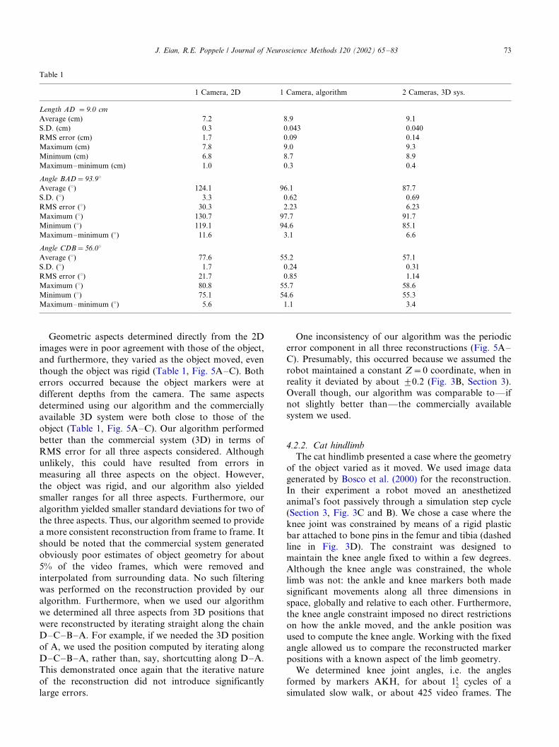
Geometric aspects determined directly from the 2D

images were in poor agreement with those of the object,

and furthermore, they varied as the object moved, even

though the object was rigid (Table 1, Fig. 5A�/C). Both

errors occurred because the object markers were at

different depths from the camera. The same aspects

determined using our algorithm and the commercially

available 3D system were both close to those of the

object (Table 1, Fig. 5A�/C). Our algorithm performed

better than the commercial system (3D) in terms of

RMS error for all three aspects considered. Although

unlikely, this could have resulted from errors in

measuring all three aspects on the object. However,

the object was rigid, and our algorithm also yielded

smaller ranges for all three aspects. Furthermore, our

algorithm yielded smaller standard deviations for two of

the three aspects. Thus, our algorithm seemed to provide

a more consistent reconstruction from frame to frame. It

should be noted that the commercial system generated

obviously poor estimates of object geometry for about

5% of the video frames, which were removed and

interpolated from surrounding data. No such filtering

was performed on the reconstruction provided by our

algorithm. Furthermore, when we used our algorithm

we determined all three aspects from 3D positions that

were reconstructed by iterating straight along the chain

D�/C�/B�/A. For example, if we needed the 3D position

of A, we used the position computed by iterating along

D�/C�/B�/A, rather than, say, shortcutting along D�/A.

This demonstrated once again that the iterative nature

of the reconstruction did not introduce significantly

large errors.

One inconsistency of our algorithm was the periodic

error component in all three reconstructions (Fig. 5A�/

C). Presumably, this occurred because we assumed the

robot maintained a constant Z�/0 coordinate, when in

reality it deviated by about 9/0.2 (Fig. 3B, Section 3).

Overall though, our algorithm was comparable to*/if

not slightly better than*/the commercially available

system we used.

4.2.2. Cat hindlimb

The cat hindlimb presented a case where the geometry

of the object varied as it moved. We used image data

generated by Bosco et al. (2000) for the reconstruction.In their experiment a robot moved an anesthetized

animal’s foot passively through a simulation step cycle

(Section 3, Fig. 3C and B). We chose a case where the

knee joint was constrained by means of a rigid plastic

bar attached to bone pins in the femur and tibia (dashed

line in Fig. 3D). The constraint was designed to

maintain the knee angle fixed to within a few degrees.

Although the knee angle was constrained, the wholelimb was not: the ankle and knee markers both made

significant movements along all three dimensions in

space, globally and relative to each other. Furthermore,

the knee angle constraint imposed no direct restrictions

on how the ankle moved, and the ankle position was

used to compute the knee angle. Working with the fixed

angle allowed us to compare the reconstructed marker

positions with a known aspect of the limb geometry.We determined knee joint angles, i.e. the angles

formed by markers AKH, for about 1/12

cycles of a

simulated slow walk, or about 425 video frames. The

Table 1

1 Camera, 2D 1 Camera, algorithm 2 Cameras, 3D sys.

Length AD �9.0 cm

Average (cm) 7.2 8.9 9.1

S.D. (cm) 0.3 0.043 0.040

RMS error (cm) 1.7 0.09 0.14

Maximum (cm) 7.8 9.0 9.3

Minimum (cm) 6.8 8.7 8.9

Maximum�/minimum (cm) 1.0 0.3 0.4

Angle BAD�93.98Average (8) 124.1 96.1 87.7

S.D. (8) 3.3 0.62 0.69

RMS error (8) 30.3 2.23 6.23

Maximum (8) 130.7 97.7 91.7

Minimum (8) 119.1 94.6 85.1

Maximum�/minimum (8) 11.6 3.1 6.6

Angle CDB�56.08Average (8) 77.6 55.2 57.1

S.D. (8) 1.7 0.24 0.31

RMS error (8) 21.7 0.85 1.14

Maximum (8) 80.8 55.7 58.6

Minimum (8) 75.1 54.6 55.3

Maximum�/minimum (8) 5.6 1.1 3.4


knee angle in the 2D video ranged from 110 to 1408 (Fig.5D) and never matched the actual angle, which was

about 1008. When we computed the knee angle after first

reconstructing the 3D positions of the markers, it

remained within 9/2.48 of 99.68 (Fig. 5D).

4.3. Effects of errors

We used the rigid object data to examine the effects of

two possible sources of error on reconstruction accu-

racy: linkage distance measurement errors and seeding

marker Z position errors. We tested these because they

are sources of error that are not present in most multi-

camera methods. We checked their effects on recon-

structed lengths, angles and positions.

We found that errors in the Z position of the seedingmarker had little effect on reconstruction accuracy. Of

course, shifting the seeding Z position caused a shift in

the Z positions of all the other markers, but their

relative positions changed little. One of the worst cases

we encountered involved object angle CDB (Fig. 3A). It

measured 568 on the object and after reconstruction was

55.28 average, S.D. 0.248. Introducing a 9/1 cm error in

the seeding marker Z position, which was about 10�/

20% of a linkage distance, resulted in only an additional

9/18 error.

On the other hand, we found that the method was

sensitive to linkage distance measurements. For exam-

ple, introducing an 11% error in length CB (9/1 cm for a

9 cm linkage) resulted in a 9/58 error in reconstructing

angle CBD. The error caused the position of C to

change little along the X and Y directions (B/0.5 cm

typically), but along the Z direction (depth) the position

of C changed by more than 10% of the linkage distance

(�/9/1 cm) in many of the images. The distance between

C and D was off by 10% on average (0.6 cm average

error in a 5.8 cm linkage). Introducing errors in other

linkage distances had similar effects.

Fig. 5. 3D reconstruction: (A�/C): Rigid object. Three reconstruction methods (see text) were compared by estimating various geometric aspects of a

rigid object. In the plots, the straight line is the actual value of the estimated aspect. Along the ordinates length units are (cm) and angle units are (8).The abscissa denotes the video frame number (60/s). (D): cat hindlimb. The knee angle was constrained to within about 9/2.58 of play (Fig. 3D). The

knee angles were computed directly from the 2D video and after 3D reconstruction using our algorithm. Ordinate is (8), abscissa is video frame

number (60/s).


5. Discussion

The single-camera method we described here per-

formed as well as a commercially available 3D recon-struction system with 2 fixed cameras. Since our

algorithm uses knowledge of linkage distances to

determine information that is typically provided by a

second camera, it is less general than multi-camera

methods. Nevertheless it has a number of advantages

including lower cost and reduced complexity. Also, set-

up for this method is simple because neither camera

position nor optical alignment need conform to anyspecifications. Thus the method may be useful in

situations where environmental constraints limit the

space available for clear camera views of the object.

The accuracy of our method is comparable with that

of a number of other methods. Miller et al. (1980) tested

their single-camera method with a moving rigid object in

a fashion similar to case A above (Section 4.2). In the

better of two tests, they reported RMS errors of 0.533cm when estimating positions. The positional RMS

error encountered using our algorithm when comparing

the initial position of D with its position determined by

iterating around a marker chain was 0.17 cm. We

encountered slightly larger RMS errors in estimating

angles (0.85 and 2.238, Section 4.2) than the 1.0, 0.8, and

0.698 reported by Miller et al.

Marzan and Karara (1975) used their multi-cameraDLT method to estimate the position of static points

and reported a standard deviation of 0.07 mm (Shapiro,

1980). In comparison, we achieved a standard deviation

of 0.9 mm in estimating the (X , Y ) coordinates of static

points, and the commercial 3D system we used exhibited

a standard deviation of 0.6 mm in estimating the same

positions (Section 4.1).

The main advantage of the multi-camera DLTmethod over single-camera methods is the DLT method

requires nothing in addition to the images for 3D

reconstruction. The 3D position of a lone marker is

determined by combining information from images

acquired from different vantage points. Also, imple-

menting the DLT method is simple because calibration

amounts to acquiring images of at least six fixed points

at known positions in space. A computer program (firstproposed by Marzan and Karara, 1975) is used to

calculate parameters that eliminate the need for addi-

tional measurements by accounting for the position and

orientation of the cameras, while also providing linear

corrections for lens distortions. Thus, given the overall

quality of the DLT method, multiple cameras are often

employed to record 3D geometry. Nevertheless, our

method can serve as a comparable substitute when costor environmental factors impose constraints.

Our method does have two possible sources of error

that are not present in standard multi-camera 3D

methods, however. These can arise from errors in

measuring distances between linked markers or from

errors in determining the Z position of the seeding

marker. In our case, the reconstruction algorithm was

robust with respect to the latter. The worst-case wefound (Section 4.3) was an additional 9/18 error in

reconstructing angle CDB (Fig. 3A) from a 9/1 cm error

in the Z position of the seeding marker, which was 10�/

20% of the object size. In this case the imaging region

was 30�/30 cm2 along X and Y at a distance of 1.5 m

from the camera along Z . Consequently, all the camera

lines of sight were nearly normal to the X �/Y planes,

and relatively large changes in Z position were requiredto induce significant changes in image locations. The

predominant effect of the seeding marker Z error was a

shift in the reconstructed Z positions of all markers by

the error.

Although the camera lines of sight were near normal

to the X �/Y planes, this did not mean the optics of the

camera could be ignored. For example, if we ignored

optics by assuming all lines of sight were normal to theimaging plane (and therefore parallel to each other),

then in Eqs. (4) and (5) parameter a would be zero so Z

position and image location would be unrelated. In such

a case, the calibration images shown in Fig. 4C and D

would be scaled versions of the predicted (X , Y )

positions of the grid markers, which we know is wrong

since their actual (X , Y ) positions were constant

throughout the calibration (Section 4.1).We examined this issue further by reconstructing 3D

object geometry while ignoring camera optics. The

assumption was the camera lines of sight were parallel

to one another and normal to the X �/Y planes. We

derived the reconstruction equations for this assumption

in Appendix C, which is the limiting case as the camera

is positioned infinitely far from the object. Those

equations are equivalent to the ones we used exceptwith parameter a , which accounts for optics, set to zero

(Section 4.1). We pursued the issue because in our case

parameter a�/0.01 was small relative to parameter b�/

0.99 (cm), and Z varied only within 9/6 cm of Z�/0

(cm), so the aZ term that accounted for optics in Eq. (4),

X�/u (aZ�/b ), was always small relative to the scaling

parameter, b . The situation was similar for related

reconstruction Eq. (5) and Eq. (6) (Section 4). Whenwe performed 3D reconstructions without accounting

for optics, i.e. with parameter a�/0, accuracy was

compromised. For example, length AD and angle

BAD were fixed on the object (Fig. 3A), and in our

3D reconstruction they varied by 0.26 cm and 3.08,respectively (Section 4.2 case A). When we ignored

optics, the values varied by 0.37 cm and 4.58, respec-

tively, a 50% increase in error. Thus, although the opticsparameter was relatively small, it was nonetheless

important for an accurate reconstruction.

The second possible source of error is the measure-

ment of linkage distances. For example, an 11% error in


length CB (9/1 cm for a 9 cm linkage), resulted in a 9/58error in the computed value of angle CDB and caused

the Z position of marker C to change by over 11%

(more than 1 cm for a 9 cm linkage) in many frames.

The large change in Z occurred because the linkage

distance error is absorbed by changing the reconstructed

position of marker C along the camera line of sight

specified by the image of C, RC (Fig. 2 and Section 2.3),

and in this case all lines of sight were nearly parallel to

the Z direction. Since in the case we examined the

linkage between C and B was nearly orthogonal to RC,

the position of C had to change along RC by a distance

that was often larger than the error in distance CB. We

expect that the method will always be sensitive to

linkage distance errors because positions are recon-

structed by finding the point along a given line of sight

that matches the linkage distance from a previously

reconstructed point.

One caveat of the method is the quadratic form of Eq.

(3). It yields for each reconstructed marker position two

Z solutions and consequently, two possible 3D posi-

tions. There is no mathematical way around this in our

algorithm. Usually though, comparison of the two

positions with the next linked marker will prove one

position degenerate, because the distance to the next

marker will be wrong for one of the two positions. A

rough knowledge of the configuration of the object may

also resolve the ambiguity. Of course, it is possible to

contrive scenarios where both positions for a marker are

viable (an example is given in Appendix B). However, in

such cases it may not be necessary to remove the

ambiguity. For example, if the marker is needed only

to build toward another marker whose position is

critical, then either position can be used. A worst-case

solution would be to use a second camera just to record

a rough estimate of the depth(s) (i.e. in front or behind)

of the ambiguous markers(s)*/but without fully inte-

grating the second camera with the imaging system.

Presumably though, in most cases a simpler more cost

effective solution would exist if the problem arose.

A motivation for using 3D imaging instead of 2D is

that subtle, yet important aspects of object geometry can

be lost when 2D images are used*/even when 3D

reconstruction appears unnecessary. For example,

Gard et al. (1996) described how out of plane rotations

of the human hip may result in errant conclusions about

gait when 2D imaging is employed. Use of this

algorithm could help resolve such issues without the

need for additional equipment.

Another potential use for the algorithm is in machine

vision guided robots. Given the linkage distances of a

robot arm, this algorithm could be used in conjunction

with a single-camera to provide and accurate estimate of

the arm position*/without the burden of multiple views

of the arm.

Acknowledgements

The authors thank G. Bosco and A. Rankin for

critical reviews of the manuscript. R. Bartosch helpedwith the figures. Also thanked are the Eian family, T.R.

Crunkinstein and W. Moch for developmental sugges-

tions, and Squantak 57 for additional help with the

figures. The work was supported by National Institute

of Neurological Disorders and Stroke grant NS-211436.

Implementation appendices

In the appendices that follow we detail the algorithm

implementation. Here, we provide an overview of the

process in the form of a recipe. Note that we use the

technical terms defined in Section 2.2 throughout the

appendices.

First acquire the calibration data as described in

Appendix A. This amounts to defining a 3D coordinate

system in the object workspace, and recording stillimages of a grid of markers moved incrementally

throughout the depth of the workspace. These images

are used to determine the image plane origin, o , as

illustrated in Fig. 4D and described Appendix A,

calibration step 2. They are also used to ascertain

realizations for the general reconstruction formulas

derived in Section 2.3 (Eq. (1) and Eq. (3)). We

derivative some parameterized realizations based ongeometric considerations in Appendix B.

Next, carry out 3D reconstruction by first determin-

ing the Z position in space of a ‘seeding marker’ on the

object. This can be done a number of ways, all of which

are described in Appendix C. Next, the (X , Y ) coordi-

nates of the seeding marker are computed given its Z

coordinate and the location of its image relative to o in

the image plane, (u , v ); realizations of Eq. (1)*/forexample, Eq. (A5) and Eq. (A6)*/are used for this

(Section 2.3). Then, the solution for Eq. (3) (for

example, Eq. (A7)) is used to compute the Z position(s)

of any marker(s) linked to the seeding marker. With the

Z position(s) of the linked marker(s) computed, the

process is repeated for the next linked marker(s).

Appendix A: Calibration and dilation formula realizations

Calibration provides the data used to determine the

image plane coordinate system ({o ; u , v}, Section 2.2)

and the realizations of the reconstruction equations

(realizations for Eq. (1) and Eq. (3), Section 2.3).

But before calibration can be performed, the spatial

directions*/X , Y , and Z */must be selected. In generaltheir orientation may be arbitrary. However, they can

often be oriented so the determination of ‘seeding’

marker is simple, and we describe this in Appendix C.


For now, we assume the spatial directions have been

selected, and we also assume the Z direction is the

coordinate direction most nearly parallel to the optical

axis of the camera. Note that the spatial origin, O , is notdefined beforehand; instead, it is determined from the

calibration. This allows us to avoid additional transfor-

mations that would otherwise complicate the recon-

struction formulas.

Calibration consists of five steps: (1) acquiring the

data; (2) determining the image plane coordinate system

{o ; u , v} and relating it to the spatial coordinates; (3)

determining the (X , Y ) position of the ‘calibration grid’(see below); (4) deriving parameterized reconstruction

formulas; and (5) determining the reconstruction equa-

tion parameters.

Step 1 is to acquire the calibration data. First, a

planar grid of markers, the calibration grid , is con-

structed (for example, see large points in Fig. 4D). The

grid should span the X �/Y portion of the object work-

space and should contain enough markers for statisticalestimation of the dilation formulas. Still images of the

grid are acquired as it is moved incrementally along the

Z direction throughout the depth of the object work-

space. The incremental distances are measured and

recorded. It is critical that the grid is oriented normal

to the Z direction. Also, the grid must be moved only

along the Z direction without changing its (X , Y )

position. However, small deviations are acceptablebecause they can be averaged out later (we achieved

satisfactory results with eyeball alignments).

Step 2 is to determine the image plane coordinate

system, {o ; u , v} (Section 2.2), and to connect it with the

spatial coordinate directions. We define the image plane

origin, o , as the image of the camera line of sight parallel

to the Z direction in space. In other words, o is the

image plane location that specifies the camera line ofsight parallel to the Z direction. We denote this line of

sight by Ro . Since Ro parallels the Z direction it has

constant X and Y coordinates, and we define X�/0 and

Y�/0 along Ro (the coordinate directions in 3D space

are selectable, but their 0 coordinates are defined based

on the calibration). Since X�/Y�/0 along Ro it contains

the origin in 3D space, O . Thus the image plane origin,

o , is the image of the spatial origin, O , and thisrelationship allows us to conveniently convert locations

in the images to positions in 3D space. We define the

Z�/0 coordinate for O by assigning one of the calibra-

tion images as acquired with the grid at Z�/0. The u

and v directions are defined as the images of the X�/0

and Y�/0 planes in space, respectively, (it follows from

the fact that o is the image of O that u and v will always

be straight lines).We locate o in the image plane using the calibration

grid images as illustrated in Fig. 4D, which shows 12

images superimposed. The point images of the markers

are grouped so all points in a group correspond to the

same marker in the grid. It may be seen that the points

in each group fall on a line, and that the lines intersect at

the point to which the images converge (Fig. 4D and B).

Since the grid is moved only along the Z direction, this

convergence point is the image of the camera line of

sight parallel to the Z direction. This point is by

definition the location of the origin, o, for the {o ; u ,

v} coordinate system.

The process of locating o is carried out statistically by

digitizing the calibration grid images. This yields the

locations of the markers in terms of the digitizer

coordinate system. A straight line is fit to each group

of points, and the digitizer coordinates of o are given by

the location that best estimates the intersection of all

these lines. All this is done in a least-squares sense.

The digitizer coordinates of o are needed to express

locations in the images in terms of the {o ; u , v}

coordinate system. The digitizer provides locations in

the video frames in terms of digitizer coordinates, and

we re-express these locations relative to o by subtracting

from them the digitizer coordinates of o . Then, if

necessary the digitizer coordinate directions are rotated

so they parallel the u and v directions from {o ; u , v}.

We use the lengths provided by the digitizer for lengths

in the {o ; u , v} coordinate system. In this way we

convert video frame locations into the {o ; u , v}

coordinate system for use with the 3D reconstruction

algorithm.

Step 3 is to determine what the 3D positions (relative

to the spatial origin, O ) of the markers in the calibration

grid were when their images were recorded. These

positions are not measured during calibration. Instead,

they are determined as follows. First, one of the grid

images is assigned as acquired at Z�/0. For example, in

our case we acquired one of the grid images with the grid

in the plane defined by the robot paths (Section 3), and

we assigned that image as acquired with the grid at Z�/

0. In this way we connected the Z�/0 position of the

‘seeding’ marker with the calibration data. The incre-

mental distances the grid was moved define the other Z

positions of the grid. This is why the grid must be

oriented normal to the Z direction: so the Z positions of

all the markers in each image are the same; this also

keeps the (X ,Y ) positions constant. We determine the

(X , Y ) positions of the markers using the ‘proportional’

locations of the marker images relative to the image

plane origin, o , and the distances between adjacent

markers in the grid. Suppose, for example, o is located 14

of the way along the u direction between two images of

markers separated by 4 cm along the X direction in the

calibration grid. Then when the grid image was

acquired, the two markers were positioned at X�/�/1

cm and �/3 cm in space, respectively. To see why,

consider Fig. A1 and these three facts: (1) by construc-

tion, Ro parallels the Z direction and has constant (X ,


Y ) coordinates (0, 0) in space; (2) o is the image of Ro

and (3) the calibration grid is always oriented normal to

the Z direction. Therefore, the grid images scale radially

about o as the Z position of the grid changes, and it

follows that the ‘proportionate’ locations of the marker

images relative to o are independent of the Z position of

the grid. We approach the Y coordinate in a similar

fashion, and use the distances between adjacent markers

in the calibration grid (measured on the grid) to work

outward from o and determine the (X , Y ) positions of

all the markers in the grid. Only one grid image is

required for this since the (X , Y ) position of the grid is

held constant as it is imaged at various Z positions.

Results from multiple images can be averaged to

improve accuracy.Step 4 is to determine candidate dilation formulas.

First, the (u , v , Z ) triplets for the dilation formula

arguments (Eq. (1), Section 2.3) are formed from the

calibration data. The location of each marker image (in

terms of the {o ; u , v} coordinate system) is coupled with

the Z position of the calibration grid when its image was

acquired. The (u , v , Z ) triplets are paired with the (X ,

Y ) position in of the marker that produced the image

(see step 3). The geometry of the camera set-up and/or

the characteristics of the (u , v , Z )�/(X , Y ) pairs are used

to ascertain candidate parameterized dilation formulas.

We derive parameterized dilation formulas based on

geometric considerations in Appendix B.

Step 5 is to estimate the candidate formula para-

meters using the (u , v , Z )�/(X , Y ) pairs (for example,

minimizing over all triplets (u , v , Z ) the sum of the

squared errors between the actual (X , Y ) position ofeach grid marker and those predicted by the candidate

dilation formula). Steps 4 and 5 can be repeated until the

simplest dilation formulas with a satisfactory fit to the

(u , v , Z )�/(X , Y ) data are achieved.

Appendix B: Derivations of parameterized dilation

formulas

Here we use geometric considerations to derive

parameterized realizations for the dilation formulas

(Eq. (1), Section 2.3). This is done first for the casewhen the optical axis of the camera is parallel to the Z

direction in space. We call this the aligned camera

scenario. Presumably, it will often be possible to align

the camera, so the corresponding dilation formulas will

be widely applicable. Note that this alignment need not

be exact to achieve acceptable results. We aligned our

camera with the Z direction by eye. We consider

arbitrary alignment below.As discussed in Section 2.3, the dilation formulas we

will derive provide (X , Y ) given (u , v , Z ), where (X , Y ,

Z ) is a position in space that appears at location (u , v ) in

the image plane. We start out by considering an

arbitrary point in the image plane, p . The location of

p , (up , vp ), specifies camera line of sight Rp that must

contain P in space that generated p in the image (Fig.

A2). Given Rp , we model how X and Y vary within Rp

as functions of Z . To do this we rely heavily on the fact

that by definition the image plan origin, o , specifies the

camera line of sight with (X , Y ) coordinates (X , Y )�/

(0, 0) (Appendix A, calibration step 2). We derive the X

and Y components of the dilation formulas by using the

slopes relative to Ro of the projections of Rp into the

X�/0 and Y�/0 planes (Fig. A2). We’ll work in the Y�/

0 plane to determine X . The determination of Y in X�/0is identical because of the radial symmetry. In Fig. A2

ray R/Y�0p is the projection of Rp into the Y�/0 plane.

We’ll denote the slope of R/Y�0p relative to Ro by MX .

For appropriately selected u* and z* we have

MX �arctanuX �u�

z�: (A1)

Since we want MX in terms of the image data, we see

from Fig. A2 that the u coordinate of the location of p ,

up in the image plane, must serve as the numerator

(u*�/up) in Eq. (A1). This forces the denominator z* to

be the distance between the camera focal point F and

the image plane origin o . If we denote this distance by 1/a , then z*�/ 1/a and from Eq. (A1) we have

MX �aup: (A2)

Fig. A1. Determining grid marker (X , Y ) positions from calibration

images: In the example depicted in the figure the image plane origin

(�/) lies 14

of the way from the left along the u direction between the two

circled marker images. If we suppose in 3D space the two circled grid

markers are separated by 4 cm along the X direction, it follows that

they must have X positions of �/1 cm and �/3 cm relative to the spatial

origin, O . See text for details. Note that this figure depicts the general

calibration case where the optical axis of the camera is not parallel to

the Z direction (i.e. not parallel with ray RO ). For the case depicted,

this causes the markers to be closer together on the left side of the

image.


The distance 1/a is used to model the optics of the

camera and is not known or measured directly. It is one

of the dilation formula parameters determined from the

calibration data (Appendix A, calibration step 5).We see from Fig. A2 that we can use MX and the

distance along Ro between F and P to determine the

distance along the X direction between P and Ro . Since

by construction (1) Ro parallels the Z direction and (2)

X�/0 along Ro , the latter distance is just the X -

coordinate of P , XP , and the former distance is along

the Z direction, so we’ll denote it by DZP,F (DZP,F not

shown in Fig. A2). We have

XP�MX (DZP;F );

and after combining this with Eq. (A2)

Xp�aup(DZP;F ): (A3)

In Eq. (A3) we need to express DZP,F in terms of ZP ,

the depth of P relative to the origin O . If we let b be a

second parameter such that b /a is the distance betweenF and O , then

DZP;F �ZP�b

a: (A4)

As with parameter a , parameter b is determined from

the calibration data (and consequently, the actual

position of O in space need not be measured). Combin-

ing Eq. (A3) and Eq. (A4) yields

Xp��

Zp�b

a

�aup:

Moving parameter a inside the parenthesis and

dropping the subscripts yields the final form of the X

component of the dilation formulas:

X �u(aZ�b)�DX (u; v;Z): (A5)

The Y component of the dilation formula is derived

similarly, and we have

Y �v(aZ�b)�DY (u; v;Z): (A6)

Both components share the same parameters a and b

because of the radial symmetry that exists when the

camera is aligned with the Z direction.

Incorporating Eq. (A5) and Eq. (A6) into the 3D

Euclidean distance formula (Eq. (2) from Section 2.3)

yields

D1;2�ffiffiffiffiffiffiffiffiffiffiffiffiffiffiffiffiffiffiffiffiffiffiffiffiffiffiffiffiffiffiffiffiffiffiffiffiffiffiffiffiffiffiffiffiffiffiffiffiffiffiffiffiffiffiffiffiffiffiffiffiffiffiffiffiffiffiffiffiffiffiffiffiffiffiffiffiffiffiffiffiffiffiffiffiffiffiffiffiffiffiffiffiffiffiffiffiffiffiffiffiffiffiffiffiffiffiffiffi[X1�u2(aZ2�b)]2� [Y1�v2(aZ2�b)]2� [Z1�Z2]2

q;

which is Eq. (3) from Section 2.3 except with the dilation

mappings (Eq. (1)) replaced with their parameterized

realizations for the aligned scenario (Eq. (A5) and Eq.

(A6)). The solution for Z2 is

By letting

a�a(X1u2�bu22�Y1v2�bv2

2)

b�1�a2(u22�v2

2)

Fig. A2. Parameterized dilation formulas for the aligned camera

scenario: The smaller figure in the upper left shows the 3D scenario.

In this case the camera is aligned with the Z direction so Ro is normal

to the image plane. The larger figure on the right is a downward view

of the Y�/0 plane in space, which is defined by rays Ro and R/Y�0P :

Point P in 3D is space is positioned at (XP , YP , ZP ). Point P? is the

projection of P into the Y�/0 plane and has position (XP , 0, ZP ).

Point p is the image of P in the image plane and has location (up , vp ).

The X position of both P and P? in space is XP and is given by XP �/

auP (ZP�/b /a ), where a and b are parameters determined from the

calibration data and aup �/tan� 1(uP ), i.e. aup is the slope of R/Y�0p

relative to Ro . YP is derived similarly. See text for details.

Z2�Z1 � a(X1u2 � bu2

2 � Y1v2 � bv22) 9

ffiffiffiffiffiffiffiffiffiffiffiffiffiffiffiffiffiffiffiffiffiffiffiffiffiffiffiffiffiffiffiffiffiffiffiffiffiffiffiffiffiffiffiffiffiffiffiffiffiffiffiffiffiffiffiffiffiffiffiffiffiffiffiffiffiffiffiffiffiffiffiffiffiffiffiffiffiffiffiffiffiffiffiffiffiffiffiffiffiffiffiffiffiffiffiffiffiffiffiffiffiffiffiffiffiffiffiffiffiffiffiffiffiffiffiffiffiffiffiffiffiffiffiffiffiffiffiffiffiffiffiffiffiffiffiffiffiffiffiffiffiffiffiffiffiffiffiffiffiffiffiffiffiffiffiffiffiffiffiffiffiffiffiffiffiffiffiffiffiffiffiffiffiffiffiffiffiffiffiffiffiffiffiffiffiffiffiffiffiffiffiffiffiffiffiffiffiffiffiffiffiffiffiffiffiffiffiffiffiffiffiffiffiffiffiffiffiffiffiffiffiffiffiffiffiffiffiffiffiffiffiffiffiffiffiffiffiffiffiffiffiffiffiffifa(X1u2 � bu2

2 � Y1v2 � bv22) � Z1g

2 � f1 � a2(u22 � v2

2)gfX 21 � 2bX1u2 � Y 2

1 � 2bY1v2 � b2(u22 � v2

2) � D21;2 � Z2

1gq

1 � a2(u22 � v2

2):


x�X 21 �2bX1u2�Y 2

1 �2bY1v2�b2(u22�v2

2)

Eq. (A7) is

Z2�Z1 � a9

ffiffiffiffiffiffiffiffiffiffiffiffiffiffiffiffiffiffiffiffiffiffiffiffiffiffiffiffiffiffiffiffiffiffiffiffiffiffiffiffiffiffiffiffiffiffiffiffiffiffiffiffiffiffiffiffiffiffiffiffiffiffiffi(a� Z1)2 � b(x� D2

1;2 � Z21)

qb

: (A7)

Eq. (A5), Eq. (A6) and Eq. (A7) are the realizations of

Eq. (1) and Eq. (3) for the aligned camera scenario. They

are used to reconstruct 3D positions just as described for

the general setting in Section 2.3, but with Eq. (1)

replaced by Eq. (A5) and Eq. (A6), and with Eq. (A7) asthe solution to Eq. (3).

One problem with Eq. (A7) is that it provides two

possible Z solutions (the 9/�). We suggest two ways to

eliminate the ambiguity. The first is to know beforehand

the relative Z position of the marker in question so the

extraneous solution can be eliminated. If this is not

possible, then both solutions can be kept until one is

proven degenerate. For example, suppose there are twoZ solutions, Z2 and Z2’ , for some P2. Then after using

the dilation formulas (Eq. (A5) and Eq. (A6), or in

general Eq. (1)) there will be two possible positions for

P2: (X2, Y2, Z2) and (X’2, Y’2, Z’2). Both (X2, Y2, Z2 )

and (X’2, Y’2, Z’2 ) can be used in Eq. (A7) (or in general

Eq. (3)) to compute Z3 for another linked point P3, and

typically the incorrect position for P2 will either (1) lead

to an imaginary square root because P2 and P3 would beseparated by a distance larger than D1,2, or (2) result in a

depth position for P3 that is obviously out of range.

It is possible to contrive scenarios where both

solutions from Eq. (A7) are non-degenerate. (Consider

the circle defined by one vertex of a triangle that is

rotated about the axis defined by its other two vertices.

Now, orient the triangle so the circle projects into a line

in the image plane. Each interior point of the linerepresents two viable solutions.) In these instances, if it

is critical that the correct position of the point in

question is known, an additional observation is re-

quired.

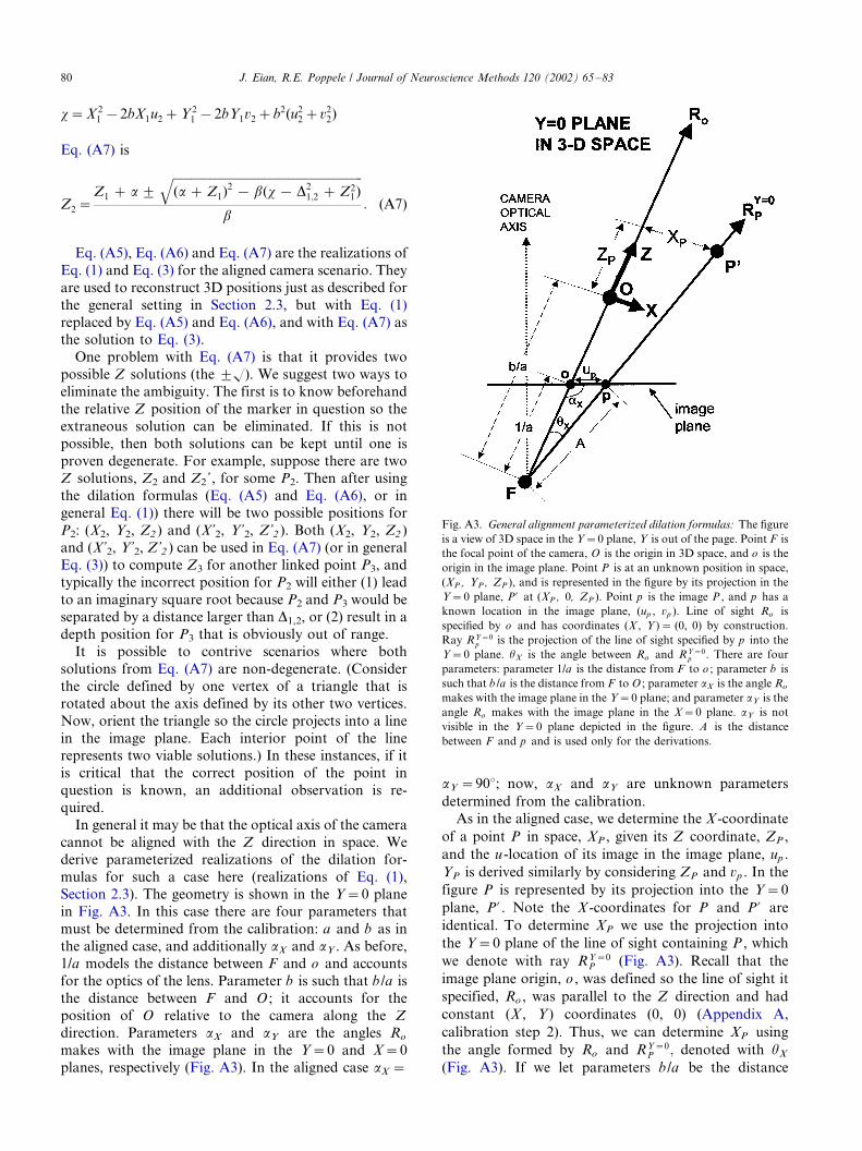
In general it may be that the optical axis of the camera

cannot be aligned with the Z direction in space. We

derive parameterized realizations of the dilation for-

mulas for such a case here (realizations of Eq. (1),Section 2.3). The geometry is shown in the Y�/0 plane

in Fig. A3. In this case there are four parameters that

must be determined from the calibration: a and b as in

the aligned case, and additionally aX and aY . As before,

1/a models the distance between F and o and accounts

for the optics of the lens. Parameter b is such that b /a is

the distance between F and O ; it accounts for the

position of O relative to the camera along the Z

direction. Parameters aX and aY are the angles Ro

makes with the image plane in the Y�/0 and X�/0

planes, respectively (Fig. A3). In the aligned case aX �/

aY �/908; now, aX and aY are unknown parameters

determined from the calibration.As in the aligned case, we determine the X -coordinate

of a point P in space, XP , given its Z coordinate, ZP ,

and the u -location of its image in the image plane, up .

YP is derived similarly by considering ZP and vp . In the

figure P is represented by its projection into the Y�/0

plane, P? . Note the X -coordinates for P and P? are

identical. To determine XP we use the projection into

the Y�/0 plane of the line of sight containing P , which

we denote with ray R/Y�0P (Fig. A3). Recall that the

image plane origin, o , was defined so the line of sight it

specified, Ro , was parallel to the Z direction and had

constant (X , Y ) coordinates (0, 0) (Appendix A,

calibration step 2). Thus, we can determine XP using

the angle formed by Ro and R/Y�0P ; denoted with uX

(Fig. A3). If we let parameters b /a be the distance

Fig. A3. General alignment parameterized dilation formulas: The figure

is a view of 3D space in the Y�/0 plane, Y is out of the page. Point F is

the focal point of the camera, O is the origin in 3D space, and o is the

origin in the image plane. Point P is at an unknown position in space,

(XP , YP , ZP ), and is represented in the figure by its projection in the

Y�/0 plane, P? at (XP , 0, ZP ). Point p is the image P , and p has a

known location in the image plane, (up , vp ). Line of sight Ro is

specified by o and has coordinates (X , Y )�/ (0, 0) by construction.

Ray R/Y�0p is the projection of the line of sight specified by p into the

Y�/0 plane. uX is the angle between Ro and R/Y�0p : There are four

parameters: parameter 1/a is the distance from F to o ; parameter b is

such that b /a is the distance from F to O ; parameter aX is the angle Ro

makes with the image plane in the Y�/0 plane; and parameter aY is the

angle Ro makes with the image plane in the X�/0 plane. aY is not

visible in the Y�/0 plane depicted in the figure. A is the distance

between F and p and is used only for the derivations.


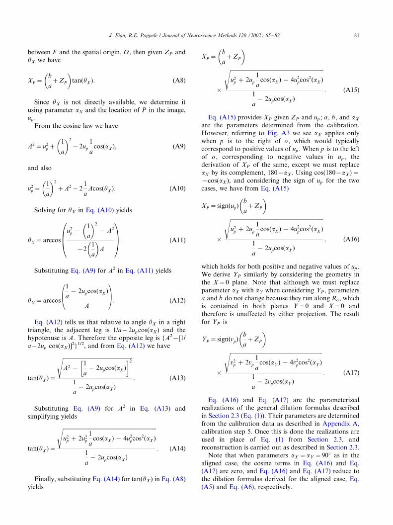
between F and the spatial origin, O , then given ZP and

uX we have

XP��

b

a�ZP

�tan(uX ): (A8)

Since uX is not directly available, we determine it

using parameter aX and the location of P in the image,

up .

From the cosine law we have

A2�u2p�

�1

a

�2

�2up

1

acos(aX ); (A9)

and also

u2p�

�1

a

�2

�A2�21

aAcos(uX ): (A10)

Solving for uX in Eq. (A10) yields

uX �arccos

�u2

p ��

1

a

�2

� A2

�2

�1

a

�A

�: (A11)

Substituting Eq. (A9) for A2 in Eq. (A11) yields

uX �arccos

�1

a� 2upcos(aX )

A

�: (A12)

Eq. (A12) tells us that relative to angle uX in a righttriangle, the adjacent leg is 1/a�/ 2upcos(aX) and the

hypotenuse is A . Therefore the opposite leg is {A2�/[1/

a�/2up cos(aX)]2}1/2, and from Eq. (A12) we have

tan(uX )�

ffiffiffiffiffiffiffiffiffiffiffiffiffiffiffiffiffiffiffiffiffiffiffiffiffiffiffiffiffiffiffiffiffiffiffiffiffiffiffiffiffiffiffiffiffiffiffiffiffiffiffiA2 �

�1

a� 2upcos(aX )

�2s

1

a� 2upcos(aX )

: (A13)

Substituting Eq. (A9) for A2 in Eq. (A13) and

simplifying yields

tan(uX )�

ffiffiffiffiffiffiffiffiffiffiffiffiffiffiffiffiffiffiffiffiffiffiffiffiffiffiffiffiffiffiffiffiffiffiffiffiffiffiffiffiffiffiffiffiffiffiffiffiffiffiffiffiffiffiffiffiffiffiffiffiffiffiffiffiffiffiffiffiu2

p � 2u2p

1

acos(aX ) � 4u2

pcos2(aX )

s

1

a� 2upcos(aX )

: (A14)

Finally, substituting Eq. (A14) for tan(uX) in Eq. (A8)

yields

XP��

b

a�ZP

�

�


p � 2up

1

acos(aX ) � 4u2

pcos2(aX )

s

1

a� 2upcos(aX )

: (A15)

Eq. (A15) provides XP given ZP and up ; a , b , and aX

are the parameters determined from the calibration.

However, referring to Fig. A3 we see aX applies only

when p is to the right of o , which would typicallycorrespond to positive values of up . When p is to the left

of o , corresponding to negative values in up , the

derivation of XP of the same, except we must replace

aX by its complement, 180�/aX . Using cos(180�/aX)�/

�/cos(aX), and considering the sign of up for the two

cases, we have from Eq. (A15)

XP�sign(up)

�b

a�ZP

�

�


p � 2up

1

acos(aX ) � 4u2

pcos2(aX )

s

1

a� 2upcos(aX )

; (A16)

which holds for both positive and negative values of up .

We derive YP similarly by considering the geometry in

the X�/0 plane. Note that although we must replace

parameter aX with aY when considering YP , parameters

a and b do not change because they run along Ro , whichis contained in both planes Y�/0 and X�/0 and

therefore is unaffected by either projection. The result

for YP is

YP�sign(vp)

�b

a�ZP

�

�

ffiffiffiffiffiffiffiffiffiffiffiffiffiffiffiffiffiffiffiffiffiffiffiffiffiffiffiffiffiffiffiffiffiffiffiffiffiffiffiffiffiffiffiffiffiffiffiffiffiffiffiffiffiffiffiffiffiffiffiffiffiffiffiffiffiffiffiv2

p � 2vp

1

acos(aY ) � 4v2

pcos2(aY )

s

1

a� 2vpcos(aY )

: (A17)

Eq. (A16) and Eq. (A17) are the parameterizedrealizations of the general dilation formulas described

in Section 2.3 (Eq. (1)). Their parameters are determined

from the calibration data as described in Appendix A,

calibration step 5. Once this is done the realizations are

used in place of Eq. (1) from Section 2.3, and

reconstruction is carried out as described in Section 2.3.

Note that when parameters aX �/aY �/908 as in the

aligned case, the cosine terms in Eq. (A16) and Eq.(A17) are zero, and Eq. (A16) and Eq. (A17) reduce to

the dilation formulas derived for the aligned case, Eq.

(A5) and Eq. (A6), respectively.


Appendix C: Seeding marker Z position

We described 3D reconstruction under the assump-

tion that the Z position of a seeding marker was known

in every image. Here we describe two methods for

determining that Z position*/and also a scenario where

the seeding marker is not even required.

The first method is to orient the spatial coordinate

system so the Z coordinate of one marker is known.

This marker is the seeding marker. For example, when a

marker remains within a plane or is affixed to an

external device, it may be possible to orient the Z

direction so the marker either maintains a constant Z

position or moves along the Z direction in a known

fashion. To determine the Z position it is necessary to

know the distance along Z between one of the calibra-

tion grid positions and the marker during imaging.

Then, if we define the aforementioned grid position as

acquired with the grid at Z�/0, the Z position of the

marker is just its Z distance from the Z�/0 grid

position. A fixed point in space, with respect to which

the Z position of the marker during imaging is known,

can be used to link the Z positions of the marker and the

calibration grid (see Section 3 for an example).In general it may be that rather than the Z coordi-

nate, the X or Y coordinate of a marker is known. Such

a marker can still serve as the seeding marker, but there

are added complications. Its Z coordinate can be

determined from the triplet (u , v , X ) or (u , v , Y ), where

u and v are its location in the images, and X or Y is

known in space. To determine Z , the discussion of the

dilation formulas (Section 2.3) is applied with Z

replaced by either X or Y , whichever is the known

coordinate. In this case one is computing (Y , Z ) from

(u , v , X ), or (X , Z ) from (u , v , Y) , rather than (X , Y )

from (u , v , Z ). Note that when the X (Y ) coordinate is

the known coordinate, the Z coordinate cannot be

computed whenever the seeding marker is in the X�/0

(Y�/0) plane because X�/0 (Y�/0) does not uniquely

define Z (consider Fig. 2).The second method for determining a seeding Z

position uses only object images and distances between

linked markers. In contrast to the first method, connec-

tions between the seeding marker Z positions and

calibration grid Z positions are not required. Any of

the calibration grid images may be assigned as acquired

with the grid at Z�/0 (Appendix A), and the Z position

of the seeding marker can still be determined from the

images alone. In this case the Z direction should be

aligned with the camera’s optical axis if possible so the

dilation formula realizations in Eq. (A5) and Eq. (A6)

apply (Appendix B).

Three markers that form a triangle of known linkage

distances are required. That is, for markers P1, P2, and

P3, the distances between P1 and P2, D1,2, P2 and P3, D2,3

and P3 and P1, D3,1, must be known (i.e. measured prior

to imaging). We use Eq. (2) three times, once for each of

the three linkages. We substitute Eq. (A5) for all Xj and

Eq. (A6) for all Yj , 10/j 0/3, to arrive at a system of

three equations and three unknowns. The unknowns are

the Zj :

The uj and vj are the coordinates of the images of the

Pj , and here a and b are the dilation formula parameters

determined from the calibration (Appendix A). From

Eq. (A7) we have the solution for Z1 in the first equation

in terms of Z2. Similarly, Eq. (A7) also provides the

solution for Z3 in the second equation in terms of Z2.

The solutions for Z1 and Z3 are substituted in the third

equation, which can then be solved numerically for the

single unknown, Z2. If multiple solutions exist, the

extraneous depths could be eliminated by repeating the

procedure with additional triplets of markers that have

only the marker in question in common. Miller et al.

(1980) described another method for determining the 3D

position of three points from a single 2D image. They

also provide suggestions for numerical solution meth-

ods.

Finally, we describe a scenario where there is no need

to know a seeding marker Z position. This occurs when

the distance between the camera and the object is large

relative to the depth of the object-imaging region. In this

case, the location of the image of a marker does not

change as its Z position varies. In essence, the camera

lines of sight are parallel within the object-imaging

region and the need for the dilation formulas is

eliminated. The 3D reconstruction problem reduces to

D1;2�ffiffiffiffiffiffiffiffiffiffiffiffiffiffiffiffiffiffiffiffiffiffiffiffiffiffiffiffiffiffiffiffiffiffiffiffiffiffiffiffiffiffiffiffiffiffiffiffiffiffiffiffiffiffiffiffiffiffiffiffiffiffiffiffiffiffiffiffiffiffiffiffiffiffiffiffiffiffiffiffiffiffiffiffiffiffiffiffiffiffiffiffiffiffiffiffiffiffiffiffiffiffiffiffiffiffiffiffiffiffiffiffiffiffiffiffiffiffiffiffiffiffiffiffiffiffiffiffiffiffiffiffiffiffiffiffiffiffiffiffiffiffiffiffi[u1(aZ1�b)�u2(aZ2�b)]2� [v1(aZ1�b)�v2(aZ2�b)]2� [Z1�Z2]2

qD2;3�

ffiffiffiffiffiffiffiffiffiffiffiffiffiffiffiffiffiffiffiffiffiffiffiffiffiffiffiffiffiffiffiffiffiffiffiffiffiffiffiffiffiffiffiffiffiffiffiffiffiffiffiffiffiffiffiffiffiffiffiffiffiffiffiffiffiffiffiffiffiffiffiffiffiffiffiffiffiffiffiffiffiffiffiffiffiffiffiffiffiffiffiffiffiffiffiffiffiffiffiffiffiffiffiffiffiffiffiffiffiffiffiffiffiffiffiffiffiffiffiffiffiffiffiffiffiffiffiffiffiffiffiffiffiffiffiffiffiffiffiffiffiffiffiffi[u2(aZ2�b)�u3(aZ3�b)]2� [v2(aZ2�b)�v3(aZ3�b)]2� [Z2�Z3]2

qD3;1�

ffiffiffiffiffiffiffiffiffiffiffiffiffiffiffiffiffiffiffiffiffiffiffiffiffiffiffiffiffiffiffiffiffiffiffiffiffiffiffiffiffiffiffiffiffiffiffiffiffiffiffiffiffiffiffiffiffiffiffiffiffiffiffiffiffiffiffiffiffiffiffiffiffiffiffiffiffiffiffiffiffiffiffiffiffiffiffiffiffiffiffiffiffiffiffiffiffiffiffiffiffiffiffiffiffiffiffiffiffiffiffiffiffiffiffiffiffiffiffiffiffiffiffiffiffiffiffiffiffiffiffiffiffiffiffiffiffiffiffiffiffiffiffiffi[u3(aZ3�b)�u1(aZ1�b)]2� [v3(aZ3�b)�v1(aZ1�b)]2� [Z3�Z1]2

q:


a non-perspective 3D distance problem. The X and Y

components of the dilation formulas become X�/DX (u ,

v , Z )�/cu and Y�/DY(u , v , Z )�/cv , where c is a

constant (determined from the calibration data) thatconverts video frame lengths into spatial lengths,

independent of Z (depth).

In this case, both a seeding marker, call it P1, and its

Z coordinate, Z1, can be selected arbitrarily. The Z

positions of all the reconstructed markers are given with

respect to Z1. Using the location of the seeding marker

in the image plane, (u1, v1), we have X1�/cu1 and Y1�/

cv1, therefore the 3D coordinates of the seeding markerare (X1, Y1, Z1)�/ (cu1, cv1, Z1). For any marker linked

to P1 by a known distance, D1,2, we use its image

location, (u2, v2), to replace X2 and Y2 in Eq. (2) with

X2�/cu2 and Y2�/cv2:

D1;2�ffiffiffiffiffiffiffiffiffiffiffiffiffiffiffiffiffiffiffiffiffiffiffiffiffiffiffiffiffiffiffiffiffiffiffiffiffiffiffiffiffiffiffiffiffiffiffiffiffiffiffiffiffiffiffiffiffiffiffiffiffiffiffiffiffiffiffiffiffiffiffiffiffiffiffiffiffi(X1�cu2)2�(Y1�cv2)2�(Z1�Z2)2

q:

Above, Z2 is the only unknown. The solution for Z2 is

Z2�Z19ffiffiffiffiffiffiffiffiffiffiffiffiffiffiffiffiffiffiffiffiffiffiffiffiffiffiffiffiffiffiffiffiffiffiffiffiffiffiffiffiffiffiffiffiffiffiffiffiffiffiffiffiffiffiffiffiffiffiffiffiffiffiffiffiffiffiffiffiffiffiffiffiffiffiffiffiffiffiffiffiffiffiffiffiffiffiffiffiffiffiffiffiffiffiffiffiffiffiD2

1;2�X 21 �2cX1u2�c2u2

2�Y 21 �2cY1v2�c2v2

2:q

(A18)

The coordinates of the linked marker are (X2, Y2,Z2)�/ (cu2, cv2, Z2). Note that Eq. (A18) is Eq. (A7)

from Appendix B with parameter a set to 0 (i.e. camera

optic ignored) and parameter b replaced by c .

References

Abdel-Aziz YI, Karara HM. Direct linear transformation from

comparator coordinates into object space coordinates in close-

range photogrammetry. Proceedings of the ASP Symposium on

Close-Range Photogrammetry 1971;1�/19.

Berstein N. Untersuching der Korperbewegungen and Korperstellun-

gen im Raum mittens Spugelaufnahmen. Arbeitsphysiologie

1930;3:3�/30.

Bosco G, Poppele RE, Eian J. Reference frames for spinal propriocep-

tion: limb endpoint based or joint-level based? J Neurophysiol

2000;83:2931�/5.

Bosco G, Poppele RE. Low sensitivity of dorsal spinocerebellar

neurons to limb movement speed. Exp Brain Res 1999;125:313�/22.

Gard SA, Knox EH, Childress DS. Two-dimensional representation of

three-dimensional pelvic motion during human walking: an exam-

ple of how projections can be misleading. J Biomech

1996;29(10):1387�/91.

Marzan GT, Karara HM. A computer program for direct linear

transformation solution of the colinearity condition and some

applications of it. Proceedings of the Symposium on Close-Range

Photogrammetric Systems 1975;420�/76.

Miller NR, Shapiro R, McLaughlin TM. A technique for obtaining

spatial kinematic parameters of segments of biomechanical systems

from cinematographic data. J Biomech 1980;13:535�/47.

Shapiro R. An overview of techniques for three-dimensional cinema-

tography. Proceedings of the Biomechanic Symposium Indiana

University October 26�/28 1980;62�/77.

Smith GA, Fewster JB. Two-dimensional panning algorithm for wide

field planar motion. Paper presented at the XVth Congress of the

International Society of Biomechanics. Finland: Jyvaskyla; July

1995.

Yu B, Koh TJ, Hay JG. A panning DLT procedure for three-

dimensional videography. J Biomech 1993;26(6):741�/51.


a single-camera method for three-dimensional video imaging

Documents