a simple spectral solar irradiance model for cloudless maritime atmospheres

A Simple Spectral Solar Irradiance Model for Cloudless Maritime AtmospheresAuthor(s): Watson W. Gregg and K. L. CarderSource: Limnology and Oceanography, Vol. 35, No. 8 (Dec., 1990), pp. 1657-1675Published by: American Society of Limnology and OceanographyStable URL: http://www.jstor.org/stable/3096598 .

Accessed: 14/06/2014 15:53

Your use of the JSTOR archive indicates your acceptance of the Terms & Conditions of Use, available at .http://www.jstor.org/page/info/about/policies/terms.jsp

.JSTOR is a not-for-profit service that helps scholars, researchers, and students discover, use, and build upon a wide range ofcontent in a trusted digital archive. We use information technology and tools to increase productivity and facilitate new formsof scholarship. For more information about JSTOR, please contact [email protected].

.

American Society of Limnology and Oceanography is collaborating with JSTOR to digitize, preserve andextend access to Limnology and Oceanography.

http://www.jstor.org

This content downloaded from 188.72.96.115 on Sat, 14 Jun 2014 15:53:32 PMAll use subject to JSTOR Terms and Conditions

http://www.jstor.org/action/showPublisher?publisherCode=limnoc

http://www.jstor.org/stable/3096598?origin=JSTOR-pdf

http://www.jstor.org/page/info/about/policies/terms.jsp


LIMNOLOGY AND

OCEANOGRAPHY

December 1990

Volume 35

Number 8

Limnol. Oceanogr., 35(8), 1990, 1657-1675 ? 1990, by the American Society of Limnology and Oceanography, Inc.

A simple spectral solar irradiance model for cloudless maritime atmospheres

Watson W. Gregg' and K. L. Carder Department of Marine Science, University of South Florida, St. Petersburg 33701

Abstract A simple spectral atmospheric radiative transfer model specific for oceanographic applications

begins with spectral extraterrestrial solar irradiance corrected for earth-sun orbital distance. Ir- radiance is then attenuated in passing through the atmosphere by Rayleigh scattering, ozone, oxygen, and water vapor absorption, and marine aerosol scattering and absorption, and is finally reduced by reflectance at the air-sea interface. The model is an extension of the continental aerosol model of Bird and Riordan, modified to include maritime aerosol properties, irradiance transmittance through the air-sea interface, and atmospheric absorption at very high spectral resolution (1 nm). Atmospheric optical constituents and the surface reflectance are functions of the local meteorological conditions, imparting flexibility to the model to reproduce the spectral irradiance under a variety of maritime atmospheres. The model computes irradiance at or just below the ocean surface at high spectral resolution in the range 350-700 nm, i.e. within the range required for photosynthetically available radiation (PAR) calculations. It agrees spectrally with observed surface spectral irradiances to within +6.6% (rms) and as integrated PAR to within +5.1%. The computed spectral irradiance is useful as an input to bio-optical models in the ocean, to phytoplankton growth and primary production models, and in remote-sensing applications.

Increasingly sophisticated phytoplankton growth and primary production models (e.g. Platt 1986), ecosystem simulation models (e.g. Walsh et al. 1988), and bio-optical models (e.g. Carder and Steward 1985; Gor- don et al. 1988b) have great potential for increasing the understanding of phytoplankton dynamics, the magnitude of oceanic primary production, and the fate of light in the sea. Use of these models to assess phytoplankton growth as a function of the

Present address: Research and Data Systems Corp., 7855 Walker Drive, Suite 460, Greenbelt, Maryland 20770.

Acknowledgments We thank T. G. Peacock and R. G. Steward at the

University of South Florida for help in obtaining the spectral irradiance observations. We also thank three anonymous reviewers for their helpful comments.

This work was supported by NASA grant NAGW- 465 and ONR grant N00014-89-J-1091.

availability of light at depth and the distribution of optical constituents requires information on light at the surface, which requires measurements or estimates of the surface light field.

Furthermore, recent advances in understanding the spectral character of light have suggested its importance in the absorption of light by phytoplankton (Sathyendranath et al. 1987), its role in primary production (Laws et al. 1990), and its effect on incu- bation methods for determining in situ primary production (Grande et al. 1989), in contrast to the conventionally used photosynthetically available radiation (PAR). Laws et al. (1990) have demonstrated for the oligotrophic ocean that ignoring the spectral character of light available for absorption by phytoplankton can result in un- derestimates of primary production rates by more than a factor of two. Until recently,

1657



Gregg and Carder

however, this approach has had limited use (see Bidigare et al. 1987; Sathyendranath and Platt 1988).

Oceanographers thus have a pressing need for spectral surface irradiance values to further the knowledge and simulation of the fate of light and primary production in the oceans, particularly where direct measurements are not available. Remotely sensed ocean chlorophyll fields from the Coastal Zone Color Scanner (CZCS) are now rou- tinely available, and primary production models using this information for initializa- tion and verification (e.g. Platt 1986; Kuring et al. 1990) require light as a forcing function. Although rigorous models of surface irradiance have been available for some time (e.g. HITRAN, Rothman et al. 1987; FAS- CODE, Clough et al. 1986; LOWTRAN, Kneizys et al. 1983), their sizes and com- putational complexities make them im- practical for many oceanographic applications. The recent version of LOWTRAN (LOWTRAN 7) contains over 18,000 lines of Fortran code and it is the smallest of the three.

Starting with Leckner (1978), a series of simple radiative transfer models has been developed (e.g. Justus and Paris 1985; Bird and Riordan 1986; Green and Chai 1988) that have found widespread applications (Green and Chai 1988). All of these simple models are specific for continental aerosols, which differ markedly in size distributions and scattering and absorption characteristics from marine aerosols (Shettle and Fenn 1979), and contain expressions for surface reflectance typical of land. Thus these models compute total and spectral irradiance fields quite different from those representing maritime atmospheres and entering the ocean.

In addition to their simplicity, these models compute separately the direct and diffuse portions of the global (direct + diffuse) irradiance, unlike the models of Tanre et al. (1979) and Gordon and Clark (1980). Sath- yendranath and Platt (1988) have shown that the directionality of the incoming irradiance is of major importance in determining the irradiance available at depth for photosynthesis.

Our purpose here is to present a simple

model developed as an extension to the above models to compute the solar irradiance at, and just below, the sea surface at very high spectral resolution (1 nm) for representative maritime conditions. We limit our model to the spectral range 350-700 nm because of its importance to phytoplankton growth and primary production and to bio- optical applications. The high spectral resolution alleviates problems in previous models, where uneven spectral intervals are used (e.g. Bird and Riordan 1986), and allows analyses on specified spectral regions. This latter consideration is of particular importance in remote-sensing applications and simulations, considering that several high spectral resolution sensors have been pro- posed for the near future (e.g. Sea-WIFS, sea wide-field-of-view sensor; MODIS, moderate resolution imaging spectrometer; and HIRIS, high resolution imaging spectrometer), each of which contains different spectral bands and widths. The limited spectral range of the model encompasses the primary spectral regions of these sensors, as well as those for bio-optical and primary production applications, and permits us to reduce the complexity of radiative transfer calculations further and therefore allows the model to be more widely useful.

The model is intended to be simple to implement but representative for maritime conditions, and it admits a variety of atmospheric aerosol turbidities and types determined by local meteorological conditions. It can be applied at any oceanic location on the surface of the earth at any time of day. It allows calculation of ifra- diance as radiant energy flux (W m-2) or explicitly as the flux of quanta or PAR (,tmol quanta m-2 s-1) if the need for quantum assessments arises (e.g. fluorescence, Ra- man scatter, and photosynthesis), as is com- mon in phytoplankton physiological simulations. PAR is formally defined here as

r700

PAR(z) = l/hc XEd(X, z) dX 350

(1)

where h is Planck's constant, c is speed of light, Ed is global downwelling irradiance, and X is wavelength in vacuo (units given in list of symbols). We follow the notation

1658



Spectral irradiance model

Significant symbols

Amplitude functions for Gathman's (1983) three-component aerosol model

Oxygen, ozone, and water vapor absorption coefficients, cm-l

Angstrom exponent Air-mass type; ranges from 1 (typical of

open-ocean aerosols) to 10 (typical of continental aerosols)

Aerosol turbidity coefficient Aerosol total extinction coefficient at

550 nm, km-' Surface drag coefficient Asymmetry parameter, an anisotropy

factor for the aerosol scattering phase function

Global downwelling solar irradiance (sum of the direct and diffuse components of the downwelling irradiance); Ed(X, 0+) is the irradiance just above the sea surface and Ed(X, 0-) is just below the sea surface, W m-2 nm-'

Direct and diffuse downwelling solar irradiance, W m-2 nm-'

Factor to account for the growth of aerosol particles with increasing relative humidity

Forward scattering probability of the aerosol (the probability that a photon will be scattered through an angle <90?)

Mean extraterrestrial solar irradiance corrected for earth-sun distance and orbital eccentricity, W m-2 nm-'

Junge exponent Aerosol scale height, km Ozone scale height, cm Mean extraterrestrial solar irradiance,

W m-2 nm-l Diffuse component of irradiance arising

from aerosol and Rayleigh scattering after molecular absorption, W m-2 nm-1

Diffuse component of irradiance arising from ground-air multiple interactions in Bird and Riordan's (1986) model; ignored in the present model, W m-2 nm-'

Wavelength in vacuo, nm Atmospheric path length, atmospheric

path length corrected for pressure, and atmospheric path length for ozone

of Gordon et al. (1983) in the CZCS atmospheric correction algorithms rather than those of atmospheric optics because of its familiarity to oceanographers.

N Number of aerosol particles, No. cm-3 n,, Index of refraction for seawater

a(X) Aerosol single-scattering albedo (an indicator of the absorption properties of the aerosol)

03 Total ozone; the amount of ozone in a 1-cm2 area in a vertical path from the top of the atmosphere to the surface; equals Hoz x 1,000, Dobson units (matm-cm)

P Atmospheric pressure; Po denotes standard pressure (1,013.25 mb), mb

PAR Photosynthetically available radiation: the flux of quanta in the wavelength range 350-700 nm, Mmol quanta m-2 s-'

r Aerosol particle radius, ,um r,o Mode radii for the three-aerosol-com-

ponent model of Gathman (1983), lum

rs, rg Surface reflectivity and ground albedo in the Bird and Riordan (1986) model; ignored in the present model

Pa Density of air, g m-3 P(0), Pp,, Direct sea-surface, direct specular sea-

Pf surface, and foam reflectance Ps, Pssp Diffuse sea-surface and diffuse specular

sea-surface reflectance RH Relative humidity, % 0 Solar zenith angle, degrees Ta(X), Transmittance after aerosol scattering

Taa(X), ancT absorption, after aerosol absorp- Tas(X) tion (not scattering), and after aerosol

scattering (not absorption) To(X), Transmittance after oxygen, ozone, and

To=(X), water-vapor absorption T,(X)

Tr(X) Transmittance after Rayleigh scattering T.(X) Transmittance after adsorption by uni-

formly mixed gases (primarily nitro- gen and oxygen)

Tr(X) Aerosol optical thickness (integral of the aerosol attenuation coefficient from the surface to the top of the atmosphere)

V Visibility, km W Instantaneous windspeed, m s-' WM Windspeed averaged over the previous

24-h period, m s-' WV Total precipitable water in a 1-cm2 area

in a vertical path from the top of the atmosphere to the surface, cm

Background Attenuation of solar irradiance in the vis-

ible and near-UV wavelengths can be at- tributed to five atmospheric processes: scat-

A,

a,(X), a,,o(X), a,

AM

c,(550)

CD (cos 0)

EJX)

Edd(X), Eds(X)

f

Fa(O)

F(X)

Ha

H, Ho= Hl(X)

a(X), I(X)

Ig(X)

x M(O), M(O),

Mo(O8)

1659



Gregg and Carder

tering by the gas mixture (Rayleigh scattering), absorption by the gas mixture (primarily by oxygen), absorption by ozone, scattering and absorption by aerosols, and absorption by water vapor. Irradiance that is not scattered but proceeds directly to the surface of the earth after losses by absorption is direct irradiance, and that which is scattered out of the direct beam but toward the surface is diffuse irradiance. The sum of the direct and diffuse components defines the global irradiance.

The present model is an extension and simplification of the Bird and Riordan (1986) model, which was designed for terrestrial applications. In their model, global downwelling irradiance at the surface is separated into its direct and diffuse components:

Ed(X) = Fo(X)cos 0 Tr(X)Ta(X)Toz(X) T(X)Tw(X)

Eds(X) = Ir(X) + Ia(X) + Ig(X) (2) (3)

where the subscripts d and s refer to direct and diffuse components, Fo(X) is the mean extraterrestrial irradiance corrected for earth-sun distance and orbital eccentricity, 0 is solar zenith angle, and Ti represents transmittance after absorption or scattering by the ith atmospheric component (see list of symbols).

In Eq. 3, Ir represents the diffuse component arising from Rayleigh scattering,

I, = Focos ToTuTwTaa(1 - Tr095)0.5 (4)

(X dependencies are now suppressed); Taa represents the transmittance after aerosol absorption (not scattering):

Taa = exp[-(l - a)raM(O)] (5)

(Justus and Paris 1985) where Wa is the single-scattering albedo of the aerosol, Ta is aerosol optical thickness, and M(0) is atmospheric path length.

Ia is the diffuse component arising from aerosol scattering,

la = Focos 0 TozTuTwTaar' 5(1 - Ta)Fa (6)

where Tas represents transmittance due to aerosol scattering only,

Tas = exp[-WaraM()] (7)

(Justus and Paris 1985), and Fa is the for-

ward scattering probability of the aerosol. Ig represents the diffuse contribution from multiple ground-air interactions:

Ig = (Edd + Ir + Ia)rsrg/( - rsrg) (8)

where r, and rg represent the sky reflectivity and ground albedo.

The model Extension of the Bird and Riordan (1986)

model to maritime atmospheres requires that a representative maritime aerosol be substituted for their continental aerosol and that reflectance at the air-sea interface be modified. The radiative transfer model presented here provides these modifications based on extensive observations and theory for maritime atmospheres. Furthermore, some simplifications to the Bird and Rior- dan model can be made based on the characteristics of the maritime environment and the spectral range under consideration, allowing easy implementation at small cost in accuracy. Finally, spectral information on extraterrestrial irradiance and atmospheric constituents is incorporated at much higher spectral resolution (1 nm) allowing flexibility to examine irradiance over any spectral interval between 350 and 700 nm. This last feature required modification of the atmospheric and extraterrestrial input parameters (absorption coefficients and solar irradiance) to the model from those described by Bird and Riordan.

Incorporating these modifications, Eq. 2 and 3 become

Edd(X, O-) = Fo(X)cos 0 Tr(X)Ta(X)Toz(X) *To(X)r(X)(1 - Pd) (9)

Eds(X, 0-) = [Ir() + a(X)](1 - P,) (10)

EA(X, 0-) = Ed(X, O-) + Eds(X, O-) (11)

where Ed(X, O-) is the downwelling irradiance just below the sea surface, Pd the direct sea-surface reflectance, p5 the diffuse reflectance, and other terms are as described in the list of symbols. In Eq. 9 and 10, Tu has been changed to To to reflect the fact that only oxygen absorbs significant irradiance within this spectral range, ground-air multiple interactions (the Ig term in Eq. 3) have been ignored because multiple sea surface-

1660




boundary-layer-atmosphere interactions are rare (Gordon and Castano 1987), and sea- surface reflectance terms specific to direct and diffuse irradiance have been added to allow for radiative transfer from the atmosphere into the ocean. The model contains only 560 lines of Fortran code, including documentation.

Extraterrestrial solar irradiance -The mean extraterrestrial solar irradiance was taken from the revised Neckel and Labs (1984) data for the region 330-700 nm (Ta- ble 1). Since these values were reported at 2-nm intervals with overlap, they were corrected for overlap and interpolated into 1-nm intervals.

The extraterrestrial irradiance corrected for earth-sun distance is given by Gordon et al. (1983) as

Fo(X) = Ho(X){1 + e cos[27r(D - 3)/365]}2 (12)

where Ho(X) is the mean extraterrestrial irradiance, e is orbital eccentricity (=0.0167) and D is day of the year (measured from 1 January).

Atmospheric path length -The slant path length through the atmosphere M(O) is required for atmospheric transmittance due to attenuation by all constituents. It may be expressed as 1/cos 0 for solar zenith angles <75?, but a correction for the sphericity of the earth-atmosphere system is required at larger zenith angles. We used the empirical formulation of Kasten (1966), which is valid at all zenith angles:

M(O) = l/[cos 0 + 0.15(93.885 - 0)- 1253].

(13) The solar zenith angle can be obtained given earth location (latitude and longitude), day of year, and time of day from standard methods (e.g. Iqbal 1983).

Ozone requires a slightly longer path length for accurate transmittance computations because its dominant concentrations are located in the stratosphere (Paltridge and Platt 1976):

Moz() = 1.0035/(cos20 + 0.007)/2. (14)

Rayleigh scattering-The Rayleigh total scattering coefficient is taken from Bird and Riordan (1986):

Tr(X) = exp[-M'(()/(115.6406X4 - 1.335X2)] (15)

where M'(O) is the path length corrected for nonstandard atmospheric pressure

M'(0) = M(0)P/P0 (16)

where Po is standard pressure. Ozone absorption-Ozone absorption co-

efficients aoz (Table 1) were taken from Inn and Tanaka (1953) and differ slightly from those tabulated by Bird and Riordan (1986) due to the higher spectral resolution here. Ozone transmittance is computed by mul- tiplying the ozone absorption coefficient by the ozone scale height Ho,

To\(X) = exp[- a0(X)Ho0zMoz()]. (17) If not otherwise known, the ozone scale heights can be estimated from the empirical climatological expression of Van Heuklon (1979).

Oxygen and water vapor absorption-Ox- ygen and water vapor absorption coefficients (ao and a,, respectively) were derived from transmittance calculations with Tanre et al.'s (1990) 5S Code (which utilized line spectra from HITRAN) with reference to the high spectral resolution transmittance observations of Kurucz et al. (1984) to obtain 1-nm resolution (Table 1). We adopted Bird and Riordan's (1986) expression for transmittance due to oxygen absorption,

Tr(X)= exp - 1.4 a0(X)M'(0) To(= exP[l + 118.3a0(X)M'(8)]45

(18) and water vapor

- -0.2385a,(X) WV M(8) T ) = ex[1 + 20.07a,(X) WV M(0)]?045

(19)

where WV is the total precipitable water vapor.

Aerosol scattering and absorption - Aero- sol concentrations and types vary widely over time and space. Consequently, accurate prediction of their optical thicknesses is difficult. Bird and Riordan (1986) specified a mean aerosol optical thickness for terrestrial atmospheres. LOWTRAN provides climatological conditions as a function of

1661



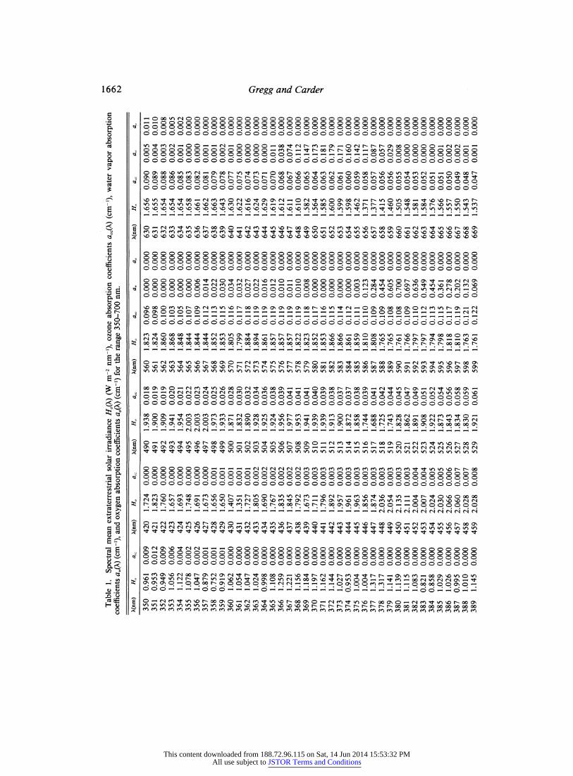
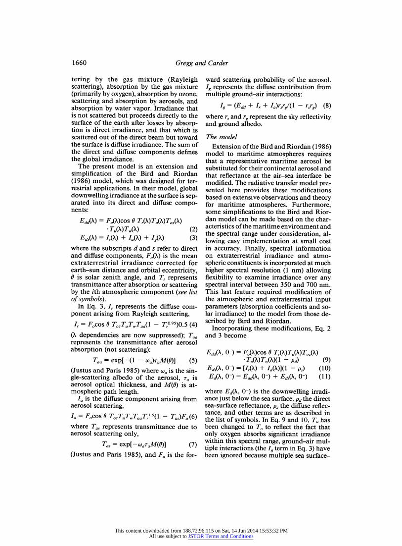
Table 1. Spectral mean extraterrestrial solar irradiance H,(X) (W m-2 nm-'), ozone absorption coefficients ao,(X) (cm-'), water vapor absorption coefficients aw(X) (cm-'), and oxygen absorption coefficients ao(X) (cm-') for the range 350-700 nm.

X(nm) Ho a,,

350 0.961 0.009 351 0.953 0.012 352 0.949 0.009 353 1.056 0.006 354 1.122 0.004 355 1.078 0.002 356 1.047 0.002 357 0.879 0.001 358 0.752 0.001 359 0.919 0.001 360 1.062 0.000 361 1.054 0.000 362 1.047 0.000 363 1.024 0.000 364 0.998 0.000 365 1.108 0.000 366 1.259 0.000 367 1.221 0.000 368 1.156 0.000 369 1.184 0.000 370 1.197 0.000 371 1.162 0.000 372 1.144 0.000 373 1.027 0.000 374 0.953 0.000 375 1.004 0.000 376 1.004 0.000 377 1.317 0.000 378 1.317 0.000 379 1.141 0.000 380 1.139 0.000 381 1.115 0.000 382 1.083 0.000 383 0.821 0.000 384 0.858 0.000 385 1.029 0.000 386 1.026 0.000 387 0.995 0.000 388 1.010 0.000 389 1.145 0.000

X(nm)

420 421 422 423 424 425 426 427 428 429 430 431 432 433 434 435 436 437 438 439 440 441 442 443 444 445 446 447 448 449 450 451 452 453 454 455 456 457 458 459

H,, a,,

1.724 0.000 1.823 0.000 1.760 0.000 1.657 0.000 1.693 0.000 1.748 0.000 1.691 0.000 1.673 0.000 1.656 0.001 1.650 0.001 1.407 0.001 1.351 0.001 1.727 0.001 1.805 0.002 1.690 0.002 1.767 0.002 1.835 0.002 1.845 0.002 1.792 0.002 1.673 0.003 1.711 0.003 1.796 0.003 1.892 0.003 1.957 0.003 1.961 0.003 1.963 0.003 1.856 0.003 1.874 0.003 2.036 0.003 2.054 0.003 2.135 0.003 2.111 0.003 2.004 0.004 2.007 0.004 2.024 0.005 2.030 0.005 2.066 0.006 2.060 0.007 2.028 0.007 2.028 0.008

h(nm) H,, a,, X(nm) Ho ao- ,, a,, 7,(nm) H,, a,, : , . a,,

490 491 492 493 494 495 496 497 498 499 500 501 502 503 504 505 506 507 508 509 510 511 512 513 514 515 516 517 518 519 520 521 522 523 524 525 526 527 528 529

1.938 0.018 1.900 0.019 1.909 0.019 1.941 0.020 1.954 0.021 2.003 0.022 2.003 0.023 2.003 0.024 1.973 0.025 1.933 0.026 1.871 0.028 1.832 0.030 1.890 0.032 1.928 0.034 1.925 0.036 1.924 0.038 1.956 0.039 1.977 0.041 1.953 0.041 1.941 0.041 1.939 0.040 1.939 0.039 1.913 0.038 1.900 0.037 1.872 0.037 1.858 0.038 1.744 0.039 1.688 0.041 1.725 0.042 1.743 0.044 1.828 0.045 1.862 0.047 1.891 0.049 1.908 0.051 1.922 0.052 1.873 0.054 1.843 0.056 1.834 0.058 1.830 0.059 1.921 0.061

560 561 562 563 564 565 566 567 568 569 570 571 572 573 574 575 576 577 578 579 580 581 582 583 584 585 586 587 588 589 590 591 592 593 594 595 596 597 598 599

1.823 0.096 0.000 0.000 1.824 0.098 0.000 0.000 1.860 0.100 0.000 0.000 1.868 0.103 0.000 0.000 1.848 0.105 0.000 0.000 1.844 0.107 0.000 0.000 1.844 0.109 0.006 0.000 1.844 0.112 0.014 0.000 1.852 0.113 0.022 0.000 1.853 0.115 0.030 0.000 1.805 0.116 0.034 0.000 1.799 0.117 0.032 0.000 1.884 0.118 0.027 0.000 1.894 0.119 0.022 0.000 1.861 0.119 0.016 0.000 1.857 0.119 0.012 0.000 1.857 0.119 0.010 0.000 1.857 0.119 0.011 0.000 1.822 0.119 0.010 0.000 1.823 0.118 0.008 0.000 1.852 0.117 0.000 0.000 1.853 0.116 0.000 0.000 1.866 0.115 0.000 0.000 1.866 0.114 0.000 0.000 1.861 0.112 0.000 0.000 1.859 0.111 0.003 0.000 1.810 0.110 0.123 0.000 1.808 0.109 0.284 0.000 1.765 0.109 0.454 0.000 1.765 0.108 0.605 0.000 1.761 0.108 0.700 0.000 1.766 0.109 0.697 0.000 1.797 0.110 0.636 0.000 1.797 0.112 0.549 0.000 1.794 0.113 0.454 0.000 1.798 0.115 0.361 0.000 1.818 0.117 0.278 0.000 1.810 0.119 0.202 0.000 1.763 0.121 0.132 0.000 1.761 0.122 0.069 0.000

630 631 632 633 634 635 636 637 638 639 640 641 642 643 644 645 646 647 648 649 650 651 652 653 654 655 656 657 658 659 660 661 662 663 664 665 666 667 668 669

1.656 0.090 0.005 0.011 1.655 0.089 0.004 0.010 1.654 0.088 0.003 0.008 1.654 0.086 0.002 0.005 1.654 0.085 0.001 0.002 1.658 0.083 0.000 0.000 1.661 0.082 0.000 0.000 1.662 0.081 0.001 0.000 1.663 0.079 0.001 0.000 1.643 0.078 0.002 0.000 1.630 0.077 0.001 0.000 1.622 0.075 0.000 0.000 1.616 0.074 0.000 0.000 1.624 0.073 0.000 0.000 1.629 0.071 0.000 0.000 1.619 0.070 0.011 0.000 1.612 0.068 0.038 0.000 1.611 0.067 0.074 0.000 1.610 0.066 0.112 0.000 1.582 0.065 0.147 0.000 1.564 0.064 0.173 0.000 1.585 0.063 0.181 0.000 1.600 0.062 0.179 0.000 1.599 0.061 0.171 0.000 1.598 0.060 0.160 0.000 1.462 0.059 0.142 0.000 1.371 0.058 0.117 0.000 1.377 0.057 0.087 0.000 1.415 0.056 0.057 0.000 1.460 0.056 0.029 0.000 1.505 0.055 0.008 0.000 1.548 0.054 0.000 0.000 1.581 0.053 0.000 0.000 1.584 0.052 0.000 0.000 1.576 0.051 0.000 0.000 1.566 0.051 0.001 0.000 1.557 0.050 0.002 0.000 1.550 0.049 0.002 0.000 1.543 0.048 0.001 0.000 1.537 0.047 0.001 0.000



1.152 1.263 1.115 0.733 0.852 1.250 1.071 0.853 1.250 1.575 1.674 1.721 1.799 1.719 1.638 1.651 1.663 1.681 1.698 1.650 1.621 1.740 1.812 1.755 1.740 1.781 1.791 1.715 1.701 1.663

0.000 0.000 0.000 0.000 0.000 0.000 0.000 0.000 0.000 0.000 0.000 0.000 0.000 0.000 0.000 0.000 0.000 0.000 0.000 0.000 0.000 0.000 0.000 0.000 0.000 0.000 0.000 0.000 0.000 0.000

2.029 2.039 2.101 2.086 1.992 1.987 1.959 1.966 2.010 2.001 1.946 1.957 2.022 2.025 2.038 2.029 1.982 1.996 2.063 2.064 2.067 2.065 2.054 2.047 2.011 1.950 1.687 1.723 1.874 1.949

0.008 0.009 0.009 0.009 0.009 0.008 0.008 0.007 0.007 0.007 0.007 0.008 0.009 0.010 0.011 0.012 0.013 0.014 0.015 0.017 0.018 0.019 0.020 0.020 0.021 0.020 0.020 0.019 0.019 0.018

1.959 1.952 1.948 1.872 1.859 1.951 1.941 1.861 1.858 1.851 1.840 1.819 1.847 1.875 1.893 1.911 1.889 1.867 1.875 1.883 1.878 1.874 1.870 1.869 1.889 1.896 1.840 1.826 1.817 1.815

0.063 0.064 0.066 0.068 0.069 0.070 0.071 0.072 0.072 0.072 0.072 0.073 0.074 0.075 0.076 0.077 0.079 0.080 0.081 0.083 0.084 0.085 0.086 0.087 0.088 0.089 0.090 0.091 0.092 0.094

1.752 1.747 1.729 1.737 1.772 1.768 1.751 1.749 1.742 1.734 1.726 1.735 1.744 1.726 1.709 1.693 1.677 1.705 1.733 1.732 1.731 1.717 1.704 1.684 1.666 1.669 1.671 1.689 1.701 1.674

0.124 0.125 0.125 0.125 0.125 0.124 0.123 0.122 0.120 0.119 0.118 0.116 0.115 0.114 0.112 0.111 0.110 0.108 0.107 0.105 0.104 0.103 0.101 0.100 0.099 0.097 0.096 0.094 0.093 0.092

0.023 0.022 0.017 0.011 0.001 0.000 0.000 0.000 0.000 0.000 0.000 0.000 0.000 0.000 0.000 0.000 0.000 0.000 0.000 0.000 0.000 0.000 0.000 0.000 0.000 0.000 0.001 0.002 0.003 0.004

0.000 0.000 0.000 0.000 0.000 0.000 0.000 0.000 0.000 0.000 0.000 0.000 0.000 0.000 0.000 0.000 0.000 0.000 0.000 0.000 0.000 0.000 0.000 0.000 0.000 0.000 0.002 0.005 0.008 0.010

1.531 1.525 1.519 1.512 1.506 1.500 1.494 1.488 1.481 1.476 1.472 1.469 1.466 1.463 1.460 1.457 1.454 1.450 1.447 1.444 1.441 1.438 1.435 1.432 1.429 1.426 1.423 1.420 1.417 1.414 1.411

0.046 0.045 0.045 0.044 0.043 0.042 0.041 0.040 0.040 0.039 0.038 0.037 0.036 0.035 0.034 0.034 0.033 0.032 0.031 0.030 0.030 0.029 0.028 0.027 0.026 0.025 0.024 0.024 0.023 0.022 0.022

0.000 0.000 0.000 0.000 0.000 0.000 0.000 0.000 0.000 0.000 0.000 0.001 0.001 0.001 0.001 0.002 0.002 0.002 0.001 0.001 0.001 0.084 0.196 0.317 0.434 0.530 0.588 0.621 0.637 0.636 0.602

0.000 0.000 0.000 0.000 0.000 0.000 0.000 0.000 0.000 0.000 0.000 0.000 0.000 0.000 0.000 0.000 0.067 0.810 0.650 0.505 0.360 0.325 0.248 0.157 0.068 0.001 0.000 0.000 0.000 0.000 0.000

390 391 392 393 394 395 396 397 398 399 400 401 402 403 404 405 406 407 408 409 410 411 412 413 414 415 416 417 418 419

460 461 462 463 464 465 466 467 468 469 470 471 472 473 474 475 476 477 478 479 480 481 482 483 484 485 486 487 488 489

530 531 532 533 534 535 536 537 538 539 540 541 542 543 544 545 546 547 548 549 550 551 552 553 554 555 556 557 558 559

600 601 602 603 604 605 606 607 608 609 610 611 612 613 614 615 616 617 618 619 620 621 622 623 624 625 626 627 628 629

670 671 672 673 674 675 676 677 678 679 680 681 682 683 684 685 686 687 688 689 690 691 692 693 694 695 696 697 698 699 700



Gregg and Carder

season (summer or winter) and region (hemispheric polar, midlatitude, or tropi- cal).

After analyzing >800 aerosol size distributions under marine conditions, however, Gathman (1983) developed the Navy marine aerosol model, which estimates the marine aerosol size distribution as well as its optical properties. Gathman's observations suggested that three aerosol components could describe the aerosol size distribution of maritime atmospheres, each a function of, and parameterized by, the local meteorological conditions. The first component describes the continental-derived component (frequently present as background even in remote marine areas), the second component represents the equilibrium sea-spray particles in the atmosphere and is related to the mean 24-h windspeed, and the third is a large, ephemeral component resulting from the current windspeed. The sizes of all three are finally related to the relative humidity to produce a description of the size distribution

3

dN/dr = Ai exp - [ln(r/froi)]2}/f (20) i=1

where Ai is an amplitude function for the component, r the radius of the aerosol, roi the mode radius for each component, and f a factor to incorporate the growth of particles with increasing relative humidity. The expression determines the change in number of particles cm-3 (dN) per increment of radius (dr).

In Eq. 20, the component amplitude function is given by

A, = 2,000(AM)2 A2 = 5.866(WM - 2.2) A3 = 0.01527(W - 2.2)R

(21) (22) (23)

10-5, their values default to these values. The mode radius of each component (roi) is designated as 0.03 utm for the first component, 0.24 ,tm for the second, and 2.0 ,im for the third (Gathman 1983). The function f relating particle size to relative humidity (RH), is given by

f= {(2 - RH/100)/[6(1 - RH/100)]}'/3 (24)

(Fitzgerald 1975). Unfortunately, determination of the op-

tical properties of the aerosol in the Navy aerosol model from the size distribution requires computation of the Mie theory extinction efficiency factors Qext and integra- tion over all aerosol radii for each wavelength. This procedure is computa- tionally expensive, especially for the 1-nm spectral resolution model required here, and thus does not conform to our intention to develop a simple model of radiative transfer.

Instead, we have developed a simplified approach that retains the major characteristics of the Navy aerosol model size distribution. In this approach, the Navy aerosol size distribution is expressed in terms of a Junge distribution (Junge 1963)

dN/dr = Cr* (25)

where y is the Junge exponent describing the slope of the aerosol size distribution and C is an amplitude function. The benefit of expressing the size distribution in terms of the Junge distribution is that the Junge exponent can be related to the Angstrom exponent in the simple, widely used, and effective Angstrom formulation for aerosol optical thickness (Van de Hulst 1981). This relationship is

a = -(y + 3) (26) where AM is the air-mass type, ranging from 1 for marine aerosol-dominated conditions to 10 for continental aerosol-dominated conditions, WM is windspeed averaged over the previous 24-h period, W is instantaneous windspeed, and R is a factor (0.05) to correct for overestimation of the large-particle amplitude based on observations of infrared transmittance (Hughes 1987). If A2 falls below 0.5 or if A3 falls below 1.4 x

(Van de Hulst 1981) where a is the Ang- strom exponent, expressing the wavelength dependence of the optical thickness in the Angstrom formulation

Ta,() = AX-a (27) (X in ,tm). / is the turbidity coefficient, representing the aerosol concentration. This formulation has gained widespread use partly because of its ability to represent rea-

1664




0 -

1- 30-

-2 -3

-2 - 1 1

log Radius (jm)

6

5_ s iJunge Distribution 5- A1 AM = 10 4-

3 3- E 2-

0

o1 -

0

-2 1 0 1

log Radius (urm)

Fig. 1. Aerosol size distributions computed by Gathman's (1983) model and the Junge distribution approximation. Size distributions are separated into the three components used by Gathman: a small but abundant background aerosol component, a medium- sized component related to the mean 24-h windspeed, and a large component related to current windspeed. This figure shows the changes in size distribution due to the air-mass type parameter and the fit by the Junge distribution.

sonably well a variety of atmospheric conditions. The Angstrom exponent may also be familiar to oceanographers who use remote sensing since it appears in the atmospheric correction algorithm for the CZCS.

By expressing the Navy aerosol size distribution in terms of the Junge distribution

3

A, exp - [ln(r/fro)]2}/f = dN/dr i=l

= Cry,

we obtain a simplified expression without losing the characteristics and meteorological dependencies of the Navy aerosol model. In practice, we further simplify by evaluating the size distribution with Eq. 20 at

only three radii: 0.1, 1.0, and 10.0 Am. We then take the logarithm of both sides of Eq. 25 and use a linear least-squares approximation to obtain the coefficient C and exponent y. This method provides an excellent representation of the size distribution over the optically important 0.1-10.0-,um radius range (Fig. 1). The Angstrom exponent is then obtained directly from Eq. 26 and is a function of the prevailing meteorological conditions.

For the calculation of /, the concentration parameter, we use the Koschmieder formula

Ca(550) = 3.91/V (28)

(Fitzgerald 1989), where Ca (550) is the aerosol total extinction coefficient at 550 nm, and V is visual range, which we assume is equal to visibility. The extinction coefficient is related to the aerosol optical thickness by

Ta(550) = c,(550)Ha (29)

where Ha is the aerosol scale height, which we assume to be 1 km (Gordon and Castano 1987). Then /, which is independent of wavelength, can be determined from Eq. 27 where X = 0.55 Aum and a is known. The aerosol optical thickness can then be computed for any wavelength. Transmittance is computed simply by

Ta(X) = exp[-,a(X)M(O)]. (30)

The Navy aerosol optical model is also tied to the visual range at 550 nm, so the models converge here. The slopes of the extinction coefficient over X computed by the two models also agree over the spectral range of interest. Thus the present model can be considered a reasonable simplification of the Navy aerosol model.

Two other aerosol characteristics are required for radiative transfer computations, Fa and Wa. As by Bird and Riordan (1986), Fa is computed from the asymmetry parameter (cos 0), which is an anisotropy factor

1665



Gregg and Carder

for the aerosol scattering phase function (Tanre et al. 1979), as a function of 0 from

Fa = 1 - 0.5 exp[(B1 + B2cos 0) *cos 0] (31)

B1 = B311.459 + B3

*(0.1595 + 0.4129B3)] (32) B2 = B3[0.0783 + B3

*(-0.3824 - 0.5874B3)] (33) B3 = ln(l - (cos 0)). (34)

The asymmetry parameter used here is a function of the aerosol size distribution, however, and thus of a

(cos 0) = -0.1417a + 0.82. (35)

For a < 0.0, (cos 0) is set to 0.82, while for a > 1.2, (cos 0) is set to 0.65. Thus for low a, typical of maritime conditions, the asymmetry parameter converges to the marine aerosol model of Shettle and Fenn (1979), and for high a, typical of continental conditions, the asymmetry parameter converges to that used by Bird and Riordan.

For the single-scattering albedo oa, we allow a dependence on both air-mass type and relative humidity

a = (-0.0032AM + 0.972) *exp(3.06 x 10-4RH). (36)

As with (cos 0), w, converges to Bird and Riordan's model under predominantly continental conditions and to Shettle and Fenn's marine aerosol model under maritime conditions.

Surface reflectance-Surface reflectance for the ocean can be divided into direct (Pd) and diffuse (ps) parts, in which the direct and diffuse irradiance are treated separately. Furthermore, each can be broken into components due to specular reflectance and reflectance due to sea foam (Koepke 1984):

Pd = Pdsp + Pf

Ps = Pssp + Pf

(37) (38)

where the subscripts sp and f refer to specular and foam reflectances, and 0 and windspeed dependencies have been suppressed.

Foam reflectance is a function of sea-surface roughness, which in turn has previously been related to windspeed (Koepke 1984). The windspeed dependence is secondary, however, the primary dependence being on

wind stress. Accordingly, using the observations of Koepke (1984), we related the sea-foam reflectance to the wind stress through

P = 0 for W < 4 m s-' (39)

Pf = DlaCDW2 - D2 for 4 < W < 7 m s-'

Pf = (D3PaCD - D4)W2 for W > 7 m s-

(40)

(41)

where Pa is the density of air (1.2 x 103 g m-3), and CD is the drag coefficient, given by

and

CD = (0.62 + 1.56W-1) x 10-3 forW < 7 ms-1

CD = (0.49 + 0.065W) x 10-3 forW> 7 ms-.

(42)

(43)

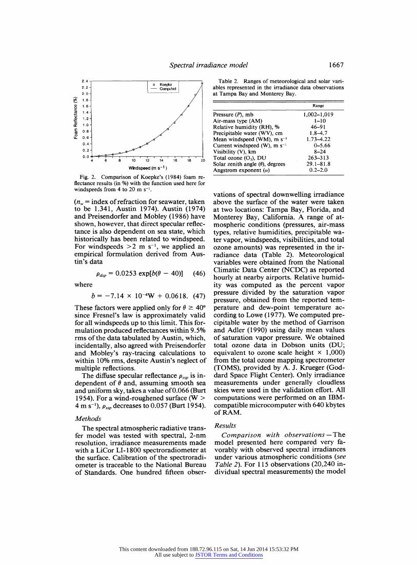
These expressions were based on those of Trenberth et al. (1989) and Koepke's observations that the foam reflectance is 0 for W < 4 m s-1. The coefficients relating wind stress to foam reflectance are D1 = 2.2 x 10-5, D2 = 4.0 x 10-4, D3 = 4.5 x 10-5, and D4 = 4.0 x 10-5. This formulation car- ries physical significance and produces an excellent representation of Koepke's results (Fig. 2). The root-mean-square (rms) error was 2.54% for the range 4-20 m s-1. By not including foam reflectance, the error in total direct reflectance at 20 m s-1 for a zenith sun was >52%; by including this formulation, the error was reduced to 1.2%. Foam reflectance is considered isotropic and thus has no dependence on 0.

Specular reflectance for direct irradiance is dependent on 0. For a flat ocean, pds(0) (and Pd since foam reflectance is zero under these conditions) can be computed directly from Fresnel's law:

1 sin2(6 - Or)

P) 2 sin2(O + Or)

+tan2(6 - Or)

tan2(6 + 0r)

(44) where 0 is the incident solar zenith angle, 0r the refracted angle, and

sin 0 nw (45)

sin Or

1666




? 1.8- / D 1 .6-

1.4-

0 _ 1.2-

E 0.8-

LL 0.6 -

0.4-

0.2-

0.0 a I I I f - I I-I I m I I f 4 6 8 10 12 14 16 18 20

Windspeed (m s-1)

Fig. 2. Comparison of Koepke's (1984) foam reflectance results (in %) with the function used here for windspeeds from 4 to 20 m s-'.

(nw = index of refraction for seawater, taken to be 1.341, Austin 1974). Austin (1974) and Preisendorfer and Mobley (1986) have shown, however, that direct specular reflectance is also dependent on sea state, which historically has been related to windspeed. For windspeeds >2 m s-1, we applied an empirical formulation derived from Aus- tin's data

dp, = 0.0253 exp[b(6 - 40)] (46)

where

b = -7.14 x 10-4W + 0.0618. (47)

These factors were applied only for 6 > 40? since Fresnel's law is approximately valid for all windspeeds up to this limit. This formulation produced reflectances within 9.5% rms of the data tabulated by Austin, which, incidentally, also agreed with Preisendorfer and Mobley's ray-tracing calculations to within 10% rms, despite Austin's neglect of multiple reflections.

The diffuse specular reflectance p, is independent of 0 and, assuming smooth sea and uniform sky, takes a value of 0.066 (Burt 1954). For a wind-roughened surface (W > 4 m s-1), p,s decreases to 0.057 (Burt 1954).

Methods The spectral atmospheric radiative trans-

fer model was tested with spectral, 2-nm resolution, irradiance measurements made with a LiCor LI-1800 spectroradiometer at the surface. Calibration of the spectroradiometer is traceable to the National Bureau of Standards. One hundred fifteen obser-

Table 2. Ranges of meteorological and solar variables represented in the irradiance data observations at Tampa Bay and Monterey Bay.

Range

Pressure (P), mb 1,002-1,019 Air-mass type (AM) 1-10 Relative humidity (RH), % 46-91 Precipitable water (WV), cm 1.8-4.7 Mean windspeed (WM), m s-' 1.734.22 Current windspeed (W), m s-' 0-5.66 Visibility (V), km 8-24 Total ozone (03), DU 263-313 Solar zenith angle (0), degrees 29.1-81.8 Angstrom exponent (a) 0.2-2.0

vations of spectral downwelling irradiance above the surface of the water were taken at two locations: Tampa Bay, Florida, and Monterey Bay, California. A range of atmospheric conditions (pressures, air-mass types, relative humidities, precipitable water vapor, windspeeds, visibilities, and total ozone amounts) was represented in the irradiance data (Table 2). Meteorological variables were obtained from the National Climatic Data Center (NCDC) as reported hourly at nearby airports. Relative humidity was computed as the percent vapor pressure divided by the saturation vapor pressure, obtained from the reported temperature and dew-point temperature ac- cording to Lowe (1977). We computed precipitable water by the method of Garrison and Adler (1990) using daily mean values of saturation vapor pressure. We obtained total ozone data in Dobson units (DU; equivalent to ozone scale height x 1,000) from the total ozone mapping spectrometer (TOMS), provided by A. J. Krueger (God- dard Space Flight Center). Only irradiance measurements under generally cloudless skies were used in the validation effort. All computations were performed on an IBM- compatible microcomputer with 640 kbytes of RAM.

Results

Comparison with observations--The model presented here compared very fa- vorably with observed spectral irradiances under various atmospheric conditions (see Table 2). For 115 observations (20,240 in- dividual spectral measurements) the model

1667



1668 Gregg and Carder

1.8 1.8 ~_- 1.6-Observed ---- 1.6 1.6 - Computed- 1.

E 14 1.4 - 14' ' -- 4

c .. 12

c 1.8- 0.8 0.8 - 0.6- 2 0.6

X 0.4 0.4

0.2 - 3 0.2-

0 0,,, 350 400 450 500 550 600 650 700 350 400 450 50 550 600 650 700

Wavelength (nm) Wavelength (nm)

1.8 1.8

1.6- 1.6-

E 1.4- 1.4-

< <6 f -- - . 0.6> W 9<s

350 400 410 500 550 600 650 700 350 Wavelength (nm) Wavelength (nm)

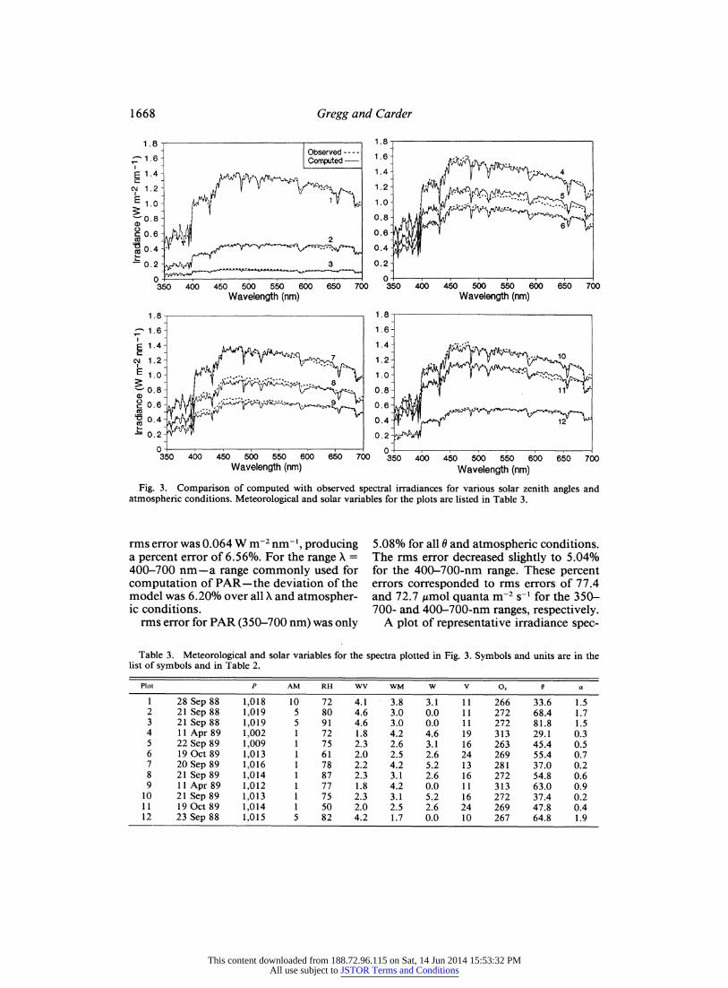
Fig. 3. Comparison of computed with observed spectral irradiances for various solar zenith angles and atmospheric conditions. Meteorological and solar variables for the plots are listed in Table 3.

rms error was 0.064 W m-2 nml, producing 5.08% for all 6 and atmospheric conditions. a percent error of 6.56%. For the range X = The rms error decreased slightly to 5.04% 400-700 nm-a range commonly used for for the 400-700-nm range. These percent computation of PAR-the deviation of the errors corresponded to rms errors of 77.4 model was 6.20% over all X and atmospher- and 72.7 mol quanta m-2 s-1 for the 350- ic conditions. 700- and 400-700-nm ranges, respectively.

rms error for PAR (350-700 nm) was only A plot of representative irradiance spec-

Table 3. Meteorological and solar variables for the spectra plotted in Fig. 3. Symbols and units are in the list of symbols and in Table 2.

Plot P AM RH WV WM W V 03 0 a

1 28 Sep 88 1,018 10 72 4.1 3.8 3.1 11 266 33.6 1.5 2 21 Sep 88 1,019 5 80 4.6 3.0 0.0 11 272 68.4 1.7 3 21 Sep88 1,019 5 91 4.6 3.0 0.0 11 272 81.8 1.5 4 11 Apr 89 1,002 1 72 1.8 4.2 4.6 19 313 29.1 0.3 5 22 Sep 89 1,009 1 75 2.3 2.6 3.1 16 263 45.4 0.5 6 19 Oct 89 1,013 1 61 2.0 2.5 2.6 24 269 55.4 0.7 7 20 Sep 89 1,016 1 78 2.2 4.2 5.2 13 281 37.0 0.2 8 21 Sep 89 1,014 1 87 2.3 3.1 2.6 16 272 54.8 0.6 9 11 Apr 89 1,012 1 77 1.8 4.2 0.0 11 313 63.0 0.9

10 21 Sep 89 1,013 1 75 2.3 3.1 5.2 16 272 37.4 0.2 11 19 Oct 89 1,014 1 50 2.0 2.5 2.6 24 269 47.8 0.4 12 23 Sep 88 1,015 5 82 4.2 1.7 0.0 10 267 64.8 1.9




Table 4. Proportions of direct, diffuse Rayleigh and aerosol, and diffuse ground multiple-interactions components computed by the Bird and Riordan (1986) model and the present model under two different combinations of visibility and air-mass type at 0 = 600. Air-mass type 10 corresponds to continental aerosols and type 1 to marine aerosols. All produce about the same total global irradiance (z208 W m-2), but the manner in which the irradiance is partitioned among components differs substantially.

Present (%)

Bird and Riordan (%) V = 16 km; AM = 10 V = 8 km; AM = 1

Direct 38 59 37 Diffuse Rayleigh + aerosols 51 41 63 Diffuse ground-air interactions 11 0 0

tra for the observations and model illus- trates the performance of the model (Fig. 3). The spectra displayed in Fig. 3 were cho- sen to represent various solar zenith angles and atmospheric conditions, which are tabulated in Table 3.

The very high spectral resolution of the model was clearly evident, and the model matched the peaks and valleys of the observed irradiances very well (Fig. 3). The depression near 590 nm in some of the observed spectra represents water-vapor absorption, which was generally well represented by the model. Occasionally, however, the model appeared to overestimate water- vapor absorption, especially for the low-humidity Monterey Bay plots. The model also appeared to match the oxygen absorption peak near 690 nm.

Comparison to Bird and Riordan's model-To compare the present model to Bird and Riordan's (1986) model we selected two widely different combinations of visibility and air-mass type that produced about the same total global irradiance as the Bird and Riordan model, which contains a fixed aerosol type and optical thickness. All other meteorological conditions (0, atmospheric pressure, precipitable water, total ozone) were held constant for the two models. The first combination corresponded to V = 16 km and an air-mass type of 10 (indicating dominance by continental aerosols). This combination produced an Angstrom exponent that, at 1.2, was similar to the Bird and Riordan model. Despite computing about the same total global irradiance (,208 W m-2) over 350-700 nm, the present model and the Bird and Riordan model partitioned irradiance components quite differently (Table 4). The present model produced more

direct irradiance than diffuse irradiance (59: 41%), and the Bird and Riordan model produced less (38:62%).

When visibility was decreased to 8 km and the air-mass type changed to 1 (typical of open-ocean aerosols), the proportions of direct and diffuse irradiances were in closer agreement to those of Bird and Riordan. Now the Angstrom exponent was 0.2-very different from that expected for continental aerosols. The total global irradiance decreased only 2 W m-2 despite the reduction of visibility by half, due to the nonabsorbing nature of marine aerosols and their strong forward scattering. Thus the Bird and Rior- dan model for continental aerosols partitioned irradiance components most closely to the present model under low visibility and maritime background aerosol.

This result stems from the contribution of ground-air multiple interactions in the Bird and Riordan model. This term was ne- glected in the present model, since it is a minor contributor to the global and diffuse irradiance (Gordon and Castano 1987). Sensitivity tests including this term in the present model with realistic ocean-surface albedo showed that its contribution never exceeded 3% at any wavelength for any windspeed up to 20 m s-~ or 0 up to 89?. The mean contribution over the 350-700- nm range, even under the worst conditions, was <1%.

This term contributed 11% of the total global irradiance at 0 = 60? in the Bird and Riordan model and up to 27% at 350 nm. It is important for terrestrial applications because of the high surface albedo of land (Bird and Riordan use 0.8) but not for the more absorbing oceans. Thus their model computed similar estimates of the global

1669



Gregg and Carder

Table 5. Sensitivity of computed surface irradiance to meteorological input parameters. The first column shows the range of the parameter under normal conditions; the second column is the rms deviation of global irradiance over the range for 350-700 nm (negative values indicate that the high end of the range produced higher irradiance); the third column is the maximal percent deviation of spectral global irradiance at any wavelength (and the wavelength at which it occurs); the fourth column is the ratio of diffuse to global irradiance (percent) at the low end of the stated range; and the fifth column is the ratio at the high end of the range. All tests were performed for 0 = 60?. Except for the variable in question, the standard conditions were: P = 1,013.25 mb, AM = 1, RH = 80%, WV = 1.5 cm, WM = 3 m s-1, W = 5 m s-', V = 10 km, 03 = 300 DU.

rms error (%) Diffuse/global (%)

Variable Range 350-700 Max/min error (%) Low High

Pressure, mb -15 to +15 0.5 0.8 56 56 (397 nm)

Air-mass type 1-10 7.4 11.2 56 54 (366 nm)

Relative humidity, % 0-99 -3.7 -4.7 55 56 (365 nm)

Precipitable water, cm 0-5 3.9 20.0 56 56 (590 nm)

Mean windspeed, m s-' 0-10 -0.2 -0.3 56 56 (358 nm)

Current windspeed, m s-' 0-20 -5.0 -7.3 55 56 (377 nm)

Visibility, km 5-25 -12.0 -15.5 79 34 (381 nm)

Total ozone, DU 100-600 7.0 13.2 56 56 (602 nm)

irradiance because it erroneously included ground-air interactions, compensating its deficiencies in characterizing the aerosol type for maritime conditions. Its proportions of the irradiance components are incorrect, a matter of importance for oceanic radiative transfer calculations. Furthermore, since these irradiance components have different spectral qualities, the Bird and Riordan model produces inaccurate estimates of the spectral irradiance entering the ocean. The model was designed for terrestrial applications, for which it performs very well, rather than the oceanic applications of interest here.

Sensitivity of the model to meteorological input parameters-The relative importance of the meteorological input parameters was tested by comparing computed surface spectral irradiances at expected ranges of the parameters under normal conditions (Table 5). Table 5 also serves as a comprehensive list of the input parameters required for the model. All sensitivity tests were performed for 0 = 60?. At this angle the atmospheric path length (1/cos 0) is double that at nadir and thus provides a reasonable representation of the optical effects of the atmospheric constituents.

Only air-mass type, visibility, and total

ozone produced differences in surface spectral irradiance that exceeded the model error over the range 350-700 nm (Table 5). Precipitable water produced a variability at the water-vapor absorption peak (590 nm) that greatly exceeded the model error, and the effect of current windspeed exceeded the model error at 377 nm. The percentage of diffuse to global irradiance (an indicator of the ratio of skylight to direct sunlight) did not differ substantially for any of the atmospheric variables except for visibility, where it went from a high of 79% for low visibility to a low of 34% for high visibility. The visibilities used here correspond to an aerosol optical thickness of 0.78 at 550 nm for 5-km visibility and to 0.16 for 25-km visibility.

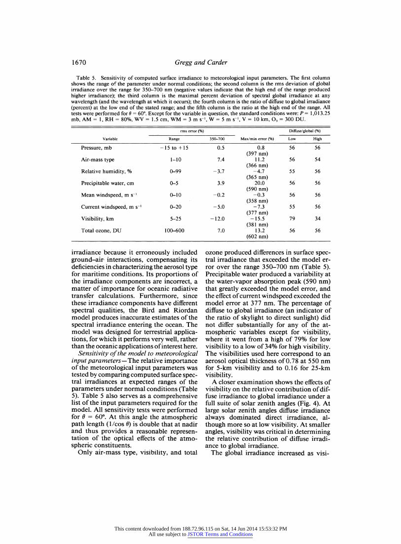
A closer examination shows the effects of visibility on the relative contribution of diffuse irradiance to global irradiance under a full suite of solar zenith angles (Fig. 4). At large solar zenith angles diffuse irradiance always dominated direct irradiance, although more so at low visibility. At smaller angles, visibility was critical in determining the relative contribution of diffuse irradiance to global irradiance.

The global irradiance increased as visi-

1670




0 *0

w

0 V w"

20 30 40 50 60 70 Solar Zenith Angle (Degrees) Solar Zenith Angle (Degrees)

Fig. 4. Computed diffuse to global irradiance ratio (%) as a function of solar zenith angle and visibility.

bility increased, but the effect was nonlin- ear. There was a greater difference between visibilities of 5 and 10 km than between 20 and 25 km. A spectral dependence on visibility also occurred; there was less change for X < 400 nm than for greater X because at small X Rayleigh scattering dominates aerosol scattering, and the irradiance here is thus less sensitive to aerosol concentrations, hence visibility.

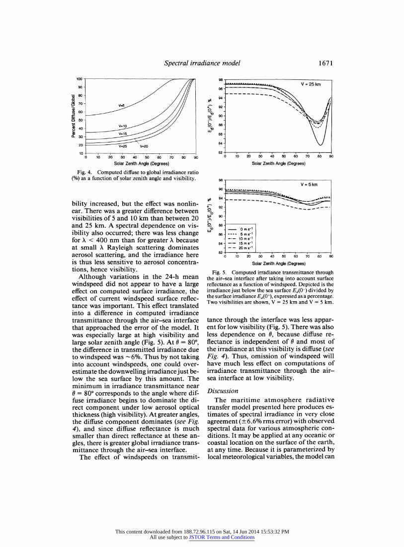
Although variations in the 24-h mean windspeed did not appear to have a large effect on computed surface irradiance, the effect of current windspeed surface reflectance was important. This effect translated into a difference in computed irradiance transmittance through the air-sea interface that approached the error of the model. It was especially large at high visibility and large solar zenith angle (Fig. 5). At 6 = 80?, the difference in transmitted irradiance due to windspeed was 6%. Thus by not taking into account windspeeds, one could overestimate the downwelling irradiance just below the sea surface by this amount. The minimum in irradiance transmittance near 0 = 80? corresponds to the angle where diffuse irradiance begins to dominate the direct component under low aerosol optical thickness (high visibility). At greater angles, the diffuse component dominates (see Fig. 4), and since diffuse reflectance is much smaller than direct reflectance at these angles, there is greater global irradiance transmittance through the air-sea interface.

The effect of windspeeds on transmit-

'a o

0

LP

96-

94-

92-

90-

88 -

86-

84-

V =5km

- ms-1 5 ms-1

-- 10 m s-1 -- 15 ms-1

- 20 m s-1

10 20 30 40 5 0 60 70 80 90

Solar Zenith Angle (Degrees)

Fig. 5. Computed irradiance transmittance through the air-sea interface after taking into account surface reflectance as a function of windspeed. Depicted is the irradiance just below the sea surface Ed(O-) divided by the surface irradiance Ed(O+), expressed as a percentage. Two visibilities are shown, V = 25 km and V = 5 km.

tance through the interface was less appar- ent for low visibility (Fig. 5). There was also less dependence on 0, because diffuse reflectance is independent of 0 and most of the irradiance at this visibility is diffuse (see Fig. 4). Thus, omission of windspeed will have much less effect on computations of irradiance transmittance through the air- sea interface at low visibility.

Discussion The maritime atmosphere radiative

transfer model presented here produces estimates of spectral irradiance in very close agreement (? 6.6% rms error) with observed spectral data for various atmospheric conditions. It may be applied at any oceanic or coastal location on the surface of the earth, at any time. Because it is parameterized by local meteorological variables, the model can

o 0

ci

0 0 a.

98

8I

1671



Gregg and Carder

be used for various atmospheric conditions. Transmittance of spectral irradiance through the air-sea interface is explicitly accounted for as a function of windspeed, thus incorporating sea-surface roughness effects on irradiance reflectance. Direct and diffuse components of the global irradiance are computed separately, and differences in atmospheric and surface conditions on these components are included, yielding a realistic assessment of the total and spectral quality of light available just below the sea surface. The model thus provides a simple but representative starting point for assess- ing the light availability of the water column and its importance to oceanic biota.

There are, however, several limitations that restrict its general use. It is designed primarily for marine aerosols and thus can be expected to produce reasonable results only over the oceans or at unpolluted coastal sites, although it can handle varying in- fluences of continental aerosols at these locations. It does not apply to visibilities restricted by fog; it is not recommended for V < 5 km because in the marine environment such conditions are usually associated with fog. It requires a cloudless day (or nearly so; <25% cloud cover probably produces negligible differences; Kasten and Czeplak 1980).

Sensitivity analyses on the eight meteorological input parameters to the model suggested their relative importance and indi- cated which of them are essential to obtain realistic downwelling irradiances. Most of the variables are easily obtainable on-board ship as well as from nearby airports, which facilitates application of the model.

Unfortunately, ozone data are important for the model and may not be generally available. A variation in total ozone from 100 to 600 DU produced a model error of 7.0% in global irradiance at 0 = 60?, and differences as large as 13% were encountered near 600 nm (near the peak ozone absorption in the visible). We obtained total ozone data from TOMS for validation of the model. The NASA Climate Data System (NCDS) makes TOMS data available within about a year of observation, but real-time data acquisition may still be a problem. The range of ozone simulated here will generally

encompass even the extreme range of values from the poles to the equator and, as such, provides an envelope. The model of Van Heuklon (1979) clearly will produce less error than the full range evaluated here. It may perform most poorly for the Antarctic ozone hole, where it tends to overestimate ozone by as much as 250 DU, but in the absence of observations the Van Heuklon model is sufficient for most purposes.

The model was relatively insensitive to a range in surface air pressure of P + 15 mb. This evaluated range is about the maximum normally encountered under clear skies (Gordon et al. 1988a). Consequently, one can assume standard pressure and ignore variations in application of this model without inducing serious error.

Variations in air-mass type did produce differences in computed surface irradiance that exceeded model error. These effects were primarily due to the change in size distribution of the aerosols. Marine aerosols are larger than continental aerosols, yielding lower absorption and more forward scattering. They thus allow more global irradiance to reach the surface than continental aerosols for the same optical thickness and change the spectral quality of the irradiance. These differences are reflected in the model through Gathman's (1983) air-mass type parameter, which ranges from 1 for marine- dominated aerosols to 10 for continental aerosols.

Determining the air-mass type is not always straightforward, however. In the open ocean a value of 1 is reliable, but in coastal areas the value depends on the origin of the prevailing air mass. Gathman suggested relating it to the atmospheric radon content, but we found that it was sufficient to take into account the wind direction in selecting the air-mass type. If the prevailing winds were from a nearby land feature and were strong and persistent, we selected a value of 10 and vice versa for sea breezes. Such determinations are relatively easy because windspeed data are required for the model anyway (for aerosol optical characteristics) and are usually accompanied by wind di- rections.

The evaluated range in relative humidity is much greater than may be expected over

1672




the oceans, where a minimum of 50% is more realistic. Even at 0 = 80?, where the effects of atmospheric properties are more pronounced, relative humidity only produced an 8.3% difference in total global irradiance from 0 to 99% RH. The low sensitivity of the model over the evaluated extreme range suggests that omitting variations in relative humidity is not serious. A reasonable mean value is 80%.

Water vapor was important to the model, however. It is related to relative humidity through the dew-point temperature, but it is difficult to find a consistent relationship between the two. Like total ozone, precipitable water data are difficult to obtain, but dew-point temperature is a commonly reported meteorological variable. We used the method of Lowe (1977) to obtain saturation vapor pressure from dew-point temperature and the method of Garrison and Adler (1990) to relate it to precipitable water. Variations in local conditions render the Garrison and Adler method valid only for monthly means, but we used the method for daily-averaged data with some success. Deviations in the model from observations near the water-vapor absorption peak (near 590 nm) in Fig. 3 are probably due to in- consistencies in the Garrison and Adler relationship on the daily time scale.

Computed surface irradiance was relatively insensitive to 24-h mean windspeed, but neglecting variations in the current windspeed can produce large error in estimates of light in the water column due to its effect on surface reflectance. In fact, assuming a flat ocean (no wind) can lead to errors in the estimation of surface specular reflectance of > 200% under 16 m s-l winds at 0 = 90? for direct irradiance. Fortunately, however, these errors in direct specular reflectance do not translate directly into errors in transmittance through the air-sea interface because most of the irradiance at large 0 is diffuse. The specular reflectance for diffuse irradiance is only slightly dependent on windspeed. Although the empirical fit used here is simplified, these types of gross errors are avoided.

Visibility was the most important input parameter to the model in terms of global irradiance, relative proportions of direct and

diffuse irradiance, and spectral quality. Un- fortunately, visibility is a rather subjective and coarse meteorological variable, being determined in practice by preselecting ob- jects at known distances and merely noting which are discernible. It is universally reported at weather stations, however, and as such is very nearly always available. Fur- thermore, it can be inferred from Fig. 4 that minor errors in visibility will produce only minor effects on estimated irradiance. There is a large and discernible difference between visibilities of 5 and 15 km even for the un- trained observer, and it is only over this range that differences are large.

Observers at remote locations or at sea stations far from land may not have access to reliable visibility estimates, however, and may have need for accurate irradiance measurements. If knowledge or estimates of the other meteorological variables can be obtained (especially windspeeds) and some type of meter (spectroradiometer, PAR meter, or pyranometer) is available, a reasonable estimate of visibility can still be made. Recall that the aerosol type (as defined by the Angstrom exponent a, forward scattering probability Fa, and single-scattering albedo Wa) can be derived from windspeed data, the air-mass type, and secondarily relative humidity. Using the meter to obtain a surface irradiance value, one can iterate through a series of visibilities until a match with the model output at 550 nm or PAR is obtained. From this numerically determined visibility, one can determine ra(550) from Eq. 28 and 29 and f from Eq. 27, which can then be used to obtain the full spectral suite of irradiances, or quanta, at the sea surface. If the visibility does not change substantially during the day, this procedure can also generate reasonable spectral irradiances (and PAR) at other times during the day without the need for further measurements. If one uses a pyranometer, the measurements must be multiplied by a factor between 0.42 and 0.5 to obtain PAR (Baker and Frouin 1987).

Consideration of the effects of visibility is critical when the direct and diffuse proportions of the global irradiance (Fig. 4) are required. Sathyendranath and Platt (1988) showed that directionality of the incoming

1673



Gregg and Carder

solar irradiance was important for computing the mean path length (average cosine) through the water column-necessary for determining the availability of light at depth. Usually the mean path length for diffuse irradiance is quite different from that of direct irradiance. The computed relative pro- portion of direct and diffuse irradiance was, except at large solar zenith angles, entirely dependent on visibility; at high visibility direct irradiance dominated, while at low visibility diffuse irradiance dominated (Fig. 4). Thus the average cosine for the water column will depend strongly on visibility.

References

AUSTIN, R. W. 1974. The remote sensing of spectral radiance from below the ocean surface, p. 317- 344. In N. G. Jerlov and E. Steemann Nielsen [eds.], Optical aspects of oceanography. Academ- ic.

BAKER, K. S., AND R. FROUIN. 1987. Relation between photosynthetically available radiation and total insolation at the ocean surface under clear skies. Limnol. Oceanogr. 32: 1370-1376.

BIDIGARE, R. R., R. C. SMITH, K. S. BAKER, AND J. MARRA. 1987. Oceanic primary production estimates from measurements of spectral irradiance and pigment concentrations. Global Biogeochem. Cycles 3: 171-186.

BIRD, R. E., AND C. RIORDAN. 1986. Simple solar spectral model for direct and diffuse irradiance on horizontal and tilted planes at the earth's surface for cloudless atmospheres. J. Climatol. Appl. Me- teorol. 25: 87-97.

BURT, W.V. 1954. Albedo overwind-roughened water. J. Meteorol. 11: 283-289.

CARDER, K. L., AND R. G. STEWARD. 1985. A remote- sensing reflectance model of a red-tide dinoflagel- late off west Florida. Limnol. Oceanogr. 30: 286- 298.

CLOUGH, S. A., F. X. KNEIZYS, E. P. SHETTLE, AND G. P. ANDERSON. 1986. Atmospheric radiance and transmittance: FASCOD2, p. 141-144. In Proc. 6th Conf. Atmospheric Radiation. Am. Meteorol. Soc.

FITZGERALD, J. W. 1975. Approximate formulas for the equilibrium size of an aerosol particle as a function of its dry size and composition and the ambient relative humidity. J. Appl. Meteorol. 14: 1044-1049.

1989. Model of the aerosol extinction profile in a well-mixed marine boundary layer. Appl. Opt. 28: 3534-3538.

GARRISON, J. D., AND G. P. ADLER. 1990. Estimation of precipitable water over the United States for application to the division of solar radiation into its direct and diffuse components. Solar Energy 44:225-241.

GATHMAN, S. G. 1983. Optical properties of the ma-

rine aerosol as predicted by the Navy aerosol model. Opt. Eng. 22: 57-62.

GORDON, H. R., J. W. BROWN, AND R. H. EVANS. 1988a. Exact Rayleigh scattering calculations for use with the Nimbus-7 Coastal Zone Color Scan- ner. Appl. Opt. 27: 862-871.

, AND OTHERS. 1988b. A semianalytic radiance model of ocean color. J. Geophys. Res. 93:10,909- 10,924.

, AND D. J. CASTANO. 1987. Coastal Zone Col- or Scanner atmospheric correction algorithm: Multiple scattering effects. Appl. Opt. 26: 2111- 2122.

, AND D. K. CLARK. 1980. Clear water radiances for atmospheric correction of Coastal Zone Color Scanner imagery. Appl. Opt. 20: 4175-4180.

, AND OTHERS. 1983. Phytoplankton pigment concentrations in the Middle Atlantic Bight: Com- parison of ship determinations and CZCS estimates. Appl. Opt. 22: 20-36.

GRANDE, K. D., AND OTHERS. 1989. Primary production in the North Pacific gyre: A comparison of rates determined by the '4C, 02 concentration and 180 methods. Deep-Sea Res. 36: 1621-1634.

GREEN, A. E. S., AND S.-T. CHAI. 1988. Solar spectral irradiance in the visible and infrared regions. Pho- tochem. Photobiol. 48: 477-486.

HUGHES, H.G. 1987. Evaluation of the LOWTRAN 6 Navy maritime aerosol model using 8 to 12 ,im sky radiances. Opt. Eng. 26: 1155-1160.

INN, E. C. Y., AND Y. TANAKA. 1953. Absorption coefficient of ozone in the ultraviolet and visible regions. J. Opt. Soc. Am. 43: 870-873.

IQBAL, M. 1983. An introduction to solar radiation. Academic.

JUNGE, C. E. 1963. Air chemistry and radioactivity. Academic.

JUSTUS, C. G., AND M. V. PARIS. 1985. A model for solar spectral irradiance at the bottom and top of a cloudless atmosphere. J. Climatol. Appl. Meteo- rol. 24: 193-205.

KASTEN, F. 1966. A new table and approximate formula for relative optical air mass. Arch. Meteorol. Geophys. Bioklimatol. B14: 206-223.

, AND G. CZEPLAK. 1980. Solar and terrestrial radiation dependent on the amount and type of cloud. Solar Energy 24: 177-189.

KNEIZYS, F. X., AND OTHERS. 1983. Atmospheric transmittance/radiance: Computer code LOW- TRAN 6. Air Force Geophys. Lab. AFGL-TR- 83-0187.

KOEPKE, P. 1984. Effective reflectance of oceanic whitecaps. Appl. Opt. 23: 1816-1824.

KURING, N., M. R. LEWIS, T. PLATT, AND J. E. O'REILLY. 1990. Satellite derived estimates of primary production on the northwest Atlantic continental shelf. Cont. Shelf Res. 10: 461-484.

KURUCZ, R. L., I. FURENLID, J. BRAULT, AND L. TESTERMAN. 1984. Solar flux atlas from 296 to 1300 nm. Natl. Solar Obs. Atlas 1.

LAWS, E. A., G. R. DITULLIO, K. L. CARDER, P. R. BETZER, AND S. HAWES. 1990. Primary production in the deep blue sea. Deep-Sea Res. 37: 715- 730.

1674




LECKNER, B. 1978. The spectral distribution of solar radiation at the earth's surface-elements of a model. Solar Energy 20: 143-150.

LOWE, P. R. 1977. An approximating polynomial for the computation of saturation vapor pressure. J. Appl. Meteorol. 16: 100-103.

NECKEL, H., AND D. LABS. 1984. The solar radiation between 3300 and 12500 A. Solar Phys. 90: 205- 258.

PALTRIDGE, G. W., AND C. M. R. PLATT. 1976. Ra- diative processes in meteorology and climatology. Elsevier.

PLATT, T. 1986. Primary production of the ocean water column as a function of surface light inten- sity: Algorithms for remote sensing. Deep-Sea Res. 33: 149-163.

PREISENDORFER, R. W., AND C. D. MOBLEY. 1986. Albedos and glitter patterns of a wind-roughened sea surface. J. Phys. Oceanogr. 16: 1293-1316.

ROTHMAN, L. S., AND OTHERS. 1987. The HITRAN database: 1986 edition. Appl. Opt. 26: 4058-4097.

SATHYENDRANATH, S., L. LAZZARA, AND L. PRIEUR. 1987. Variations in the spectral values of specific absorption of phytoplankton. Limnol. Oceanogr. 32:403-415.

,AND T. PLATT. 1988. The spectral irradiance field at the surface and in the interior of the ocean: A model for applications in oceanography and remote sensing. J. Geophys. Res. 93: 9270-9280.

SHETTLE, E. P., AND R. W. FENN. 1979. Models for

the aerosols of the lower atmosphere and the effects of humidity variations on their optical properties. Air Force Geophys. Lab. Tech. Rep. AFGRL-TR-79-0214.

TANRE, D., C. DEROO, P. DUHAUT, M. HERMAN, AND J. J. MORCRETTE. 1990. Description of a computer code to simulate the satellite signal in the solar spectrum: The 5S code. Int. J. Remote Sens- ing 11: 659-668.

, M. HERMAN, P. Y. DESCHAMPS, AND A. DE LEFFE. 1979. Atmospheric modeling for space measurements of ground reflectances, including bidirectional properties. Appl. Opt. 18: 3587-3594.

TRENBERTH, K. E., W. G. LARGE, AND J. G. OLSEN. 1989. The effective drag coefficient for evaluating wind stress over the oceans. J. Climatol. 2: 1507- 1516.

VAN DE HULST, H. C. 1981. Light scattering by small particles. Dover.

VAN HEUKLON, T. K. 1979. Estimating atmospheric ozone for solar radiation models. Solar Energy 22: 63-68.

WALSH, J. J., D. A. DIETERLE, AND M. B. MEYERS. 1988. A simulation analysis of the fate of phytoplankton within the Mid-Atlantic Bight. Cont. Shelf Res. 8: 757-788.

Submitted: 17 July 1989 Accepted: 23 May 1990

Revised: 8 October 1990

1675



a simple spectral solar irradiance model for cloudless maritime atmospheres

Documents