a simple, solar spectral model for direct-normal and diffuse horizontal irradiance

Solar Energy, Vol. 32, No. 4, pp. 461~,71, 1984 0038-092X/84 $3.00 + .00 Printed in Great Britain. © 1984 Pergamon Press Ltd.

A SIMPLE, SOLAR SPECTRAL MODEL FOR DIRECT-NORMAL AND DIFFUSE

HORIZONTAL IRRADIANCE

RICHARD E. BIRD Solar Energy Research Institute; 1617 Cole Blvd., Golden, CO 80401, U.S.A.

(Received 28 November 1982; accepted 28 April 1983)

Abstraet--A spectral model for cloudless days that uses simple mathematical expressions and tabulated look-up tables to generate direct-normal and diffuse horizontal irradiance is presented. The model is based on modifications to previously published simple models and comparisons with rigorous radiative transfer codes. This model is expected to be more accurate than previous simple models and applicable to a broader range of atmospheric conditions. The primary significance of this model is its simplicity, which allows it to be used on small desk-top computers. The spectrum produced by this model is limited to 0.3--4.0 ~m wavelength with an approximate resolution of 10 nm.

I. INTRODUCTION

Solar spectral data for a wide range of atmospheric conditions at the earth's surface are required for solar energy device development and performance evaluation. In the past, detailed studies have been performed using the results from rigorous radiative transfer codes for the diffuse component[l-3]. This has seriously limited the use of accurate modeled data, because these rigorous codes are complex and require large computing capabili- ties. To alleviate this problem, we have been investigat- ing methods of simplifying the rigorous codes by using a single homogeneous layer, and we have attempted to use a simple Beer's law approach that has met with limited previous success [4-7].

We have determined that very accurate results can be obtained for calculations at the earth's surface with a single homogeneous layer model. This greatly reduces the computation time for a rigorous deterministic model, and we believe that it would be possible to produce a model that would be easy to use with little knowledge of atmospheric physics or meteorology. Such a model would make rigorous calculations possible for a much larger group of researchers, but it would still require substantial computer capacity. This type of model could be used only at the surface, or possibly at the top, of the atmosphere, but not at points between the atmospheric boundaries.

We have pursued the second approach of using a Beer's law formalism that is based on the work of Leckner [6] and Brine and Iqbal [7]. With this approach, a very simple model might be produced that could be used for surface calculations on microcomputers. In the following material, we present the model that has evolved from modifying the models previously men- tioned, such that our results agree well with those from the rigorous codes.

Id~ = Ho~ T,~ To~ To~ Tw~ Tu~. (1)

Equation (1) can be multiplied by cos z, where z is the solar zenith angle, to obtain the direct irradiance on a horizontal surface. The extraterrestrial spectral irradiance Hox at the mean solar distance based on the Neckel and Labs spectrum [8] is used here. A modified and extended version of this spectrum, obtained from Frohlich and Werli of the World Radiation Center, Davos, Swit- zerland, is actually used in this model. Wavelengths were selected based on measured spectra [9] at a total of 122 wavelengths between 0.3 and 4.0gin to reproduce a spectrum of aproximately 10 nm spectral resolution. The extraterrestrial spectrum takefi from a 10-nm-resolution spectrum is given in Table 1 along with absorption coefficients for the 122 wavelengths.

T,~, Tax, To~, T~, and T,~ are the transmittance functions for Rayleigh scattering, aerosol extinction, ozone absorption, water vapor absorption, and absorption by the uniformly mixed gases (oxygen and carbon dioxide), respectively.

3. RAYLEIGHT SCATTERING

We began this work by using the Leckner expression [6] for Rayleigh scattering transmittance, but we found that it produced results that deviated from Pendorf's data [10]. We adapted the expression from LOWTRAN 5 [11], which agrees very closely with Pendorf. This expression is

T,x = exp { - M'/[A4(115.6406- 1.335/A2)]}, (2)

where M' is the pressure-corrected air mass. The relative air mass given by Kasten [12] is

M = [cos(Z) + 0.15(93.885 - Z)-12531 I, (3)

2. DIRECT NORMAL IRRADIANCE

The irradiance on a surface normal to the direction of the sun at ground level for a wavelength A gm is

where Z is the apparent solar zenith angle. The pressure- corrected air mass is M ' = MP/Po where Po = 1013 mb and P is the measured surface pressure in rob. Kasten's

461

462 R. E. BraD

Table 1. The nickel and labs revised extraterrestrial spectrum and atmospheric absorption coefficients at 122 wavelengths

Extraterrestrlal Extraterrestrial Wavelength

Spe trum Wavelength Spe trum um ( W/m~/um ) awl a°k auk Um (W/m~/Um) awx a°~ aul

0 . 3 0 0 5 3 5 . 9 0 6 . 6 9 0 0 . 9 8 0 7 6 7 , 0 1 . 1 0 0 0 0 . 3 0 5 5 5 8 . 3 0 5 , 5 0 0 0 . 9 9 3 5 7 5 7 . 6 0 . 1 0 0 0 . 3 1 0 6 2 2 . 0 0 2 . 7 0 0 1 . 0 4 6 8 8 . 1 0 . 0 0 0 0 1 0 0 0.315 692.7 0 1.35 0 1.07 640.7 0.001 0 0 0.320 715.1 0 0.800 0 1.10 606.2 3.4 0 0 0.325 832.9 0 0.380 0 1.12 585.9 60.0 0 0 0.330 961.9 0 0.160 0 1.13 570.2 30.0 0 0 0 . 3 3 5 9 3 1 . 0 0 0 . 0 9 5 ~ 1 . 1 3 7 5 6 4 . 1 3 3 . 0 0 O 0.340 900.6 0 0.040 0 1.161 544.2 7.0 0 0 0.345 911.3 0 0.019 0 1.17 533.4 3.5 0 0 0 . 3 5 0 9 7 5 . 5 0 0 . 0 0 7 0 1 . 2 0 5 0 1 . 6 2 . 0 0 0 0 . 3 6 0 9 7 5 . 9 0 O 0 1 . 2 4 4 7 7 . 5 0 . 0 0 2 0 0 . 1 5 0.370 1119.9 0 0 0 1.27 442.7 0.002 0 0.25 0.380 1103.8 0 0 0 1.29 440.0 0.I 0 0.02 0.390 1033.8 0 0 0 1.32 416.8 4.0 0 0;0002 0.400 1479.1 0 0 0 1.35 391.4 200.0 0 O.O0011 0.410 1701.3 0 0 0 1.395 358.0 lO00.O 0 O.O0001 0.420 1740.4 0 0 0 1.4425 327.5 i00.0 0 0.29 0.430 1587.2 0 0 0 1.4625 317.5 40.0 0 0,011 0.440 1837.0 0 0 0 1.477 307.3 40.0 0 0.005 0.450 2005.0 0 0.003 0 1.497 300.4 4.0 0 0.0006 0.460 2043.0 0 0.006 0 1.520 292.8 0.16 O 0 0.470 1987.0 0 0.009 0 1.539 275.5 0.002 0 0.005 0.480 202?.0 0 O.014 0 1.558 272.1 O.001 ~ 0.13 0.490 1896.0 0 0.021 0 1.578 259.3 %0001 0 0.04 0.500 1909.0 0 0.030 O 1.592 246.9 0.00001 0 0.06 0.510 1927.0 0 0.040 0 1.610 244.0 0.0001 0 0.13 0.520 1831.0 0 0.048 0 1.630 243.5 0.001 0 OiO01 0.530 1891.0 0 0.063 0 1.646 234.8 0.01 0 0.0014 0.540 1898.0 0 0.075 0 1.678 220.5 0.036 0 0£000,i 0.550 1892.0 0 0.095 0 1.740 190.8 i.i 0 0.00001 0.570 1840.0 0 0.120 0 1.80 171.1 60.0 0 0.00001 0.593 1768.0 0.075 0.119 0 1.860 144.5 600.0 0 0.0001 0.610 1728.0 0 0.132 0 1.920 135.7 700.0 0 0.001 0.630 1658.0 O 0.120 0 1.960 123.0 50.0 0 4.3 0.656 1524.0 0 0.065 0 1.985 123.8 2.0 0 O.13 0.6676 1531.0 0 0.060 0 2.005 113.0 1.5 0 21.0 0.690 1420.0 0.016 0.028 0.30 2.035 108.5 1.0 0 O.13 0.710 1399.0 0.05 0.018 0 2.065 97.5 0.4 0 1.0 0.718 1374.0 1.80 0.015 0 2.10 92.4 0.20 0 0.08 0.7244 1373.0 1.0 0.012 0 2.148 82.4 0.25 0 0.001 0.740 1298.0 0.025 O.010 0 2.198 74.6 ~.33 0 0.00038 0.7525 1269.0 0.005 0.008 0 2.270 68.3 0.02 0 0.001 0.7575 1245.0 0.O001 0.007 0 2.360 63.8 4.0 0 0.0005 0.7625 1223.0 0.00001 0.006 4.0 2.450 49.5 80.0 0 0.00015

, O . 7 6 7 5 1 2 0 5 . 0 0 . O 0 0 0 1 0 . 0 0 5 0 . 3 5 2 . 5 4 8 . 5 . 3 1 0 . 0 0 0 . 0 0 0 1 4 0 . 7 8 0 1 1 8 3 . 0 0 . 0 0 0 3 0 0 2 . 6 3 8 . 6 1 5 0 0 0 . 0 0 0 . 0 0 0 6 6 0.800 1148.0 0.0125 0 0 2.7 36.6 22000.0 0 i00.0 0.816 I091.0 1.45 0 0 2.8 32.0 8000.0 0 150.0 0.8237 1062.0 2.1 0 0 2.9 28.1 .650.0 0 0.13 0.8315 1038.0 0.155 0 0 3.0 24.8 240.0 0 0.0095 0.840 1022.0 0.061 0 0 3 .1 2 2 . 1 230.0 0 0.001 0.860 998.7 0.00001 0 0 3.2 19.6 I00.0 0 0.8 0.880 947.2 0.0026 O 0 3.3 17.5 120.0 0 1.9 0 . 9 0 5 8 9 3 , 2 1 . 0 0 0 0 3 . 4 1 5 . 7 1 9 . 5 0 1 . 3 O . 9 1 5 8 6 8 . 2 2 . 0 0 0 3 . 5 1 4 . 1 3 . 6 0 0 . 0 7 5 O. 925 829.7 1.0 0 0 3,6 12.7 3. I 0 0.01 0.930 830.3 15.0 Q 0 3.7 11.5 2.5 0 0.00195 0.937 814.0 34.0 Q. 0 3.8 10.4 1.4 0 0.004 0.948 786.9 20.0 0 0 3.9 9.5 o.17 0 0.29 0.965 768.3 3.4 0 0 4.0 8.6 0.0045 0 0.025

expression for relative air mass will be used in all calculation performed here unless otherwise noted.

Using Rayleigh scattering theory[13], Pendorf's data can be generated with a depolarization factor of 0.035. Young [14] concludes that the correct value should be 0.0279. Results will show that eqn (2), when used in conjunction with other expressions presented later, will produce data that agree very well with data from the BRITE radiative transfer code. A depolarization factor of 0.0279 was used in the BRITE code. Because of the good agreement, no adjustments have been made in equation 2 to reflect the new depolarization factor.

4. AEROSOL SCATTERING AND ABSORPTION

Aerosol scattering and absorption (extinction) are determined in one calculation procedure in the rigorous codes using MIE [13] scattering theory. These time-

consuming calculations require a knowledge of the aerosol particle size distribution and the particle complex index of refraction as a function of wavelength. The rural aerosol model [15] has been used in our rigorous calculations. The aerosol size distribution for this model is shown in Fig. 1, and it is a bimodal, log-normal size distribution. The complex index of refraction for several wavelengths is presented in Table 2, along with the single scattering albedo and the asymmetry factor for the aerosol model.

Leckner [6] uses an approximate formalism of Ang- strom [16] to express the aerosol optical depth (turbidity) as a function of wavelength. This formalism assumes that the turbidity versus the wavelength on a log-log plot is linear. King and Herman [17], and our unpublished measurements, show that the turbidity often exhibits curvature on a log-log plot. In fact, the rural aerosol model shows curvature [15]. As a result of this, we have

E

O Z

>,

a

.ID E

Z

10 s

10 6

104

102

10 0

1 0 :

10 4

10 6

0 I

Dg @

• . * ° ° ° ° . ° °

.° n~(r)*

Solar spectral model for direct-normal and diffuse horizontal irradiance

Rura l M o d e l

n , ( r ) *

10 8 ~ 10 3 10 2 10 ~ 10 0 10 ~ 10 ~

Rad ius (lJm) The two dotted lines represent the individual log-normal

distributions which combine to make up the rural model

Fig. 1. Aerosol particle size distribution for rural aerosol model.

463

Table 2. Optical parameters of the rural aerosol model at selected wavelengths

)(a) nl(b ) n2(C ) Wo(d) <cos 8> (e)

0 . 3 0 5 1 . 5 3 0 . 0 0 8 0 . 9 2 8 0 0 . 6 6 3 6 0 . 3 1 1 .53 0 .0072 0 .9337 O.6612 0 . 3 2 1 . 5 3 0 . 0 0 6 9 0 .9356 0 .6596 0 . 3 3 1 . 5 3 0 .0059 0 . 9 4 3 0 0 .6581 0 . 3 5 1 . 5 3 0 . 0 0 5 9 0 . 9 4 2 6 0 . 6 5 5 5 0 . 4 0 1 .53 0 .0059 0 .9423 O.6511 0 . 4 5 1 . 5 3 0 . 0 0 5 9 0 . 9 4 1 6 0 . 6 4 7 4 0 . 5 0 1 .53 0 .0059 0 . 9 4 0 4 0 .6436 0 . 5 5 1 .53 0 . 0 0 6 6 0 . 9 3 3 3 0 .6397 0 . 6 5 1 .53 0 .0068 0 . 9 2 9 3 0 .6352 0 . 7 5 1 . 5 2 7 0 . 0 0 8 2 7 0 . 9 1 4 4 0 . 6 3 3 3 0 . 8 0 1 .521 0 .00989 0 . 9 0 2 0 0 .6329 0.84 1.521 0.0104 0.8932 0.6333 0.90 1.520 0.0115 0.8820 0.6323 0.95 1.520 0.0124 0.8728 0.6313 1.1 1.516 0.0147 0.8438 0.6307 1.29 1.496 0.0163 0.8178 0.6382 1.395 1.48g 0.0172 0.8022 0.6421 1.52 1.478 0.0184 0.7823 0.6479 1.61 1.474 0.0173 0.7845 0.6503 1.80 1.421 0.0143 0.7835 0.6794 2.198 1.350 0.0108 -- 0.71

(a)x = wavelength (~m).

(b)n I = real refractive index.

(C)n 2 = imaginary refractive index.

(d)w o = single scattering albedo.

(e)<cos O> = asymmetry factor.

used the multiterm Angstrom formalism, as follows:

"r,,~, =/3,X -'~".

The turbidity coefficients/3,, are directly proportional to the turbidity, and the coefficients a , are related to the aerosol size distribution. The slope of the line on a log-log plot of turbidity versus wavelength is given by a. By using two a 's , a line with two straight segments can be formed to approximate a curved line. Table 3 presents values of/3, and/32 for the different turbidities used in this work. The two values of a used for the rural aerosol model are ot1=1.0274 between 0.3 and 0.5gm wavelength and a2 = 1.2060 between 0.5 and 4.0v, m wavelength. A new value of/3 can be formed by

/3. =/3o~'./~'o,

where/3, is the new value,/3o is old value for a given a, and ~', and ro are the new and old values, respectively, of the turbidity at 0.5/~m wavelength. The transmittance function for aerosols is then given by

Ta~, = exp [ -/3,A - " M ] ,

where awx is the water vapor absorption coefficient at the wavelength ;t and w is the precipitable water in cm in

(4) a vertical path. See Table 1 for the values of awx used here.

Unfortunately, this work was begun by using the water vapor expression given in a preprint copy of Brine's and Iqbal's paper [7] that contained transposed numbers. The number 0.3285 in eqn (7) was 0.2385 in Leckner's paper. We used the transposed number to derive water vapor absorption coefficients that agree well with BRITE data for 1.42cm of precipitable water. The error was dis- covered later when large differences with SOLTRAN 5 data were found for other water vapor amounts. The transposed form of the equation provided good results for all air mass values, and it was determined that with the original equation, we would still have problems with

(5) changing water vapor amounts. So that new absorption coefficients would not have to be determined, the transposed form of the equation was retained and a correction for water vapor amount was derived. Data discussed later will support this approach.

Note that the BRITE code derives its absorption coefficients from the 1978 Air Force Geophysics

(6)

with the values of /3. and a , changing at 0 .5gm wavelength.

5. WATER VAPOR ABSORPTION

A modified version of the water vapor transmittance expression of Leckner [6] was arrived at for use in this model, namely

T,~, = exp{- 0.3285 a~,x[w + (1.42- w)0.5]M /(1.0 + 20.07aw~,M) °'5} (7)

Table 3. Angstrom turbidity coefficients for several turbidities in the rural aerosol model

Ta (0.5 ~m) B I 6 2

0.I 0.0490 0.0433

0.27 0.1324 0.1170

0.37 0.1814 0.1603

0.51 0.2501 0.2210

464 R. E. BIRD

Laboratories line parameter data [18] for use in its band absorption model. The data were degraded to 20cm -1 resolution for use in BRITE. It would be desirable to have the resolution constant in wavelength rather than wave number for this application, but it was beyond the scope of this work to do that. As an alternative, we have selected wavelengths that appear to reproduce 10-nm- resolution experimental data. A few absorption coefficients have been adjusted to agree with experimental data where they vary from the results of the rigorous codes.

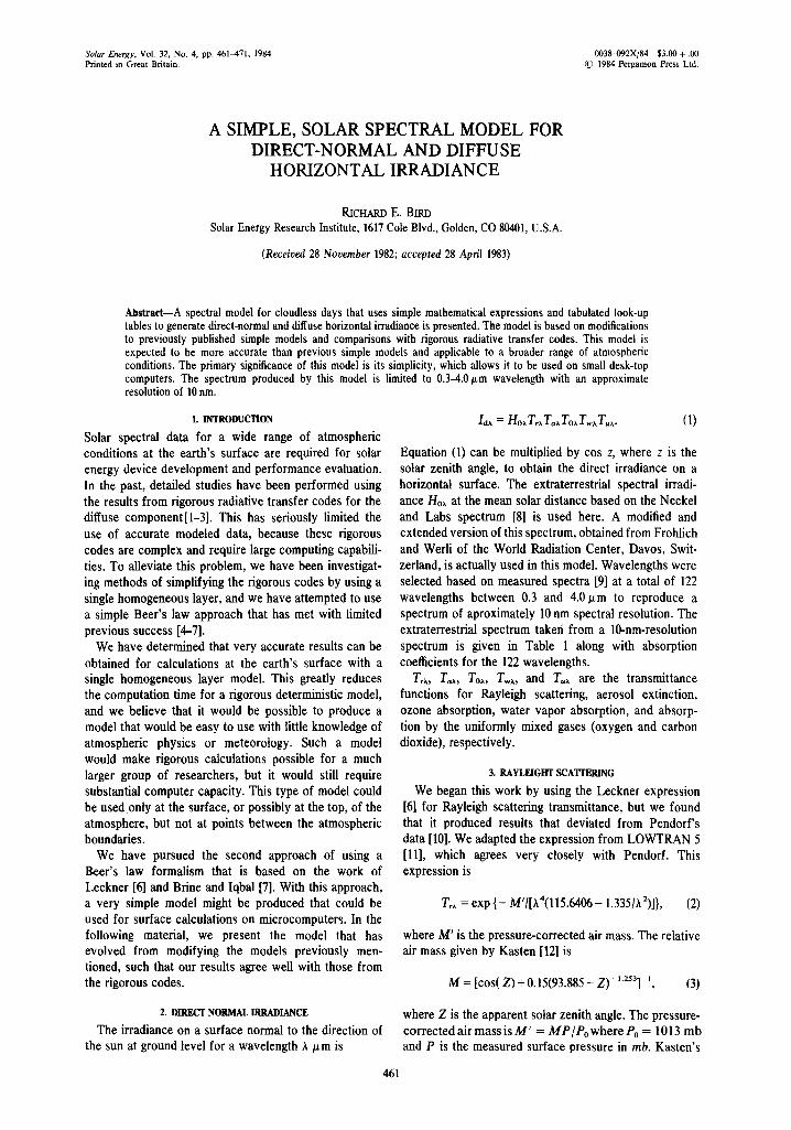
Table 4. Diffuse correction factor for r,(0.5) = 0.1

;k O* 37* 48 .19" 60* 70* 75* 80*

0.30 0.75 0.75 0.76 0.85 1.20 1.30 1.4 0.35 0.99 0.98 0.99 1.01 1.08 1.17 1.4 0.40 i.i i. II l.ll 1.12 1.20 1.27 1.52 0.45 1.04 1.06 1.06 1.06 i.ii 1.16 1.34 0.50 1.08 1.06 1.05 1.04 1.09 I.Ii 1.23 0.55 1.04 1.02 1,00 1.00 1.04 1.04 1.13 0.71 1.29 1.19 1.17 1.09 1.04 0.97 0.93 0.78 1.2 i.ii 1,08 1.01 1.00 0.93 0.94 0.9935 1.06 0.98 0.95 0.86 0.86 0.80 0.83 2.1 0.69 0.73 0,75 0.68 0.72 0,65 0.68 4.1 0.69 0.73 0.75 0.68 0.72 0.65 0.68

6. OZONE AND UNIFORMLY MIXED GAS ABSORPTION

The ozone transmittance equation of Leckner [7] was used, which is

To~ = exp [ - aox 03 Mo]. (8)

aox is the ozone absorption coefficient at wavelength A shown in Table 1, 03 is the ozone amount in a vertical 0.30

0.35 path in cm, an M, is the air mass expression for ozone 0.40 given by Paltridge and Platt [19]. 0.45

.0.50 0.55

M. = 35.0/[ 1224.0 cos2(z) + 1] °5. (9)

The formalism of Van Heuklon [20] can be used to determine ozone amount if data are not available.

Leckner's expression [7] for the uniformly mixed gases was used here:

Table 5. Diffuse correction factor for tJ0.5) = 0.27

k O* 37* 48.19" 60* 70" 75* 80*

0.71 0 .78 0.9935 2.1 4.1

0.88 0.93 1.02 1.23 2.00 4.00 6.3 1.08 1.07 i . i i 1.19 1 .51 1.97 3.76 I.ii 1.13 1.18 1.24 1.46 1.70 2.61 1.04 1.05 1.09 1.11 1.24 1.34 1.72 1.15 1.O0 l.O0 0.99 1.06 1.07 1.22 1.12 0.96 0.96 0.94 0.99 0,96 1.04 1.32 1.12 1.07 1.02 l.lO 0.90 0.80 1.23 1,09 1.05 1.07 1.00 0.85 0.78 0.98 0.94 0.91 0.83 0 . 9 0 0.79 0.74 0.69 0.68 0.71 0.64 0 .70 0.59 0.52 0.69 0.68 0.71 0.64 0 .70 0.59 0.52

118.93 a ,xM) ], T.x = exp [ - 1.41 a,,~.M'/(1 + ,045

(10)

where aux is the absorption coefficient and the gaseous amount combination shown in Table 1, and M' is the pressure-corrected air mass discussed earlier.

7. DIFFUSE HORIZONTAL IRRADIANCE

Historically, the diffuse irradiance has been difficult to put in simple terms with any confidence, because it is much more difficult to compute rigorously than the direct component. The methods of Brine and Iqbal[7], which are based on the broadband methods of Davies and Hays [21], were the starting point for this work. The equation for the scattered component on a horizontal surface at wavelength A is

h~ = (L~ +IaD C~ + I~, (11)

Table 6. Diffuse correction factor for r,(0.5) = 0.37

O* 37* 48.19" 60 ° 70 ° 75* 80*

0 .3 0.88 0.89 0.94 1.11 1.84 3.96 12.2 0 .35 1.16 1.00 1.09 1.23 1.65 2 .40 5.47 0.4 1.13 1,19 1.41 1.30 1,51 2.03 2.87 0.45 1.08 i,i0 1.30 1.16 1.26 1.34 1.72 0.5 1.18 1,04 1.03 1.O1 1.13 1.12 1.27 0.55 1.15 1,01 0.99 0.96 1.06 1.02 1.07 0.71 1.33 1.12 1.06 1.02 1.00 0.88 0.80 0.78 1.05 1,03 0.98 0.89 0.92 0.79 0.75 0.9935 0.94 1.O0 0.88 0.82 0.90 0.80 0.77 2.1 0.76 0,78 0.84 0.70 0.77 0.69 0.57 4.1 0.76 0,78 0.84 0.70 0.77 0.69 0.57

where I,~ is the Rayleigh scattered irradiance on a horizontal surface at wavelength A, Iax is the aerosol scattered component on a horizontal surface at wavelength A, Igx is the ground/air reflected irradiance on a horizontal surface at wavelength ~., and Cx is a correction factqr that is wavelength- and zenith-angle- dependent. The correction factor CA is shown in Tables 4-7 for four different turbidities and seven solar zenith angles. The following equations apply:

Irx = H, cos (Z) To~,T,~Tw~,T,,x(I - T,~)0.5 (12)

I,~ = Hocos(Z) ToxT,xTwxT, x (1 - T,,JWoF,, (13)

Table 7. Diffuse correction factor for ra(0.5)= 0.51

l 0 ° 37 ° 4 8 . 1 9 " 60 ° 7 0 " 75 ° 80 °

0.3 0.88 0.99 1.02 1.22 2.26 5.17 31.3 0.35 1.08 i.ii 1.28 1.27 1.80 2.76 7.48 0.40 1.06 1.09 1.29 1.12 1.36 1.67 2.78 0.45 1.01 1.03 1.20 1,00 i. II 1.20 1,57 0.5 1.21 1.06 1.01 0.99 1.04 1.02 1.17 0.55 1.20 1.02 0.97 0.95 0.97 0.92 0.98 0.71 1.21 1.09 1.04 0.95 0.94 0.82 0.71 0.78 1.14 0.97 0.96 0,88 0.92 0.77 0.68 0.9935 0,98 0.99 0.93 0.84 0.89 0.73 0.69 2.1 0.69 0.63 0.71 0,73 0.81 0.72 0.78 4.1 0.69 0.63 0.71 0.73 0.81 0.72 0.78

Solar spectral model for direct-normal and diffuse horizontal irradiance 465

I~ = [l~, cos (Z ) + (I,,~ + L D C ~ ] p , o , I ( I - p~p,)

ps = T;~,T ' , ,T~, , [T'x(1 - T'x)0.5 + Tb , (1 - T'~)0.22 Wo].

(14)

(15)

The albedo of the air is Ps, and the primes on the transmittance terms indicate that they are evaluated at an air mass of 1.9. The ground albedo is Og; Wo is the single scattering albedo of the aerosol; and Fa is the forward to total scattering ratio of the aerosol. Fo = (1 + (cos 0))0.5 where (cos O) is the asymmetry factor of the aerosol. The value of Wo used for the rural aerosol is 0.928, and the value of Fa is 0.82. Equations (11)-(15) are identical to those of Brine and Iqbal [7] except for the correction factor C~.

An attempt was made to modify eqns (11)-(14) so that simple equations could be used without the use of correction tables. However, all attempts to fit the equations to a set of data for several turbidities and zenith angle combinations were unsuccessful. We concluded that, even though the equations gave fairly accurate results for some conditions, it was impossible to get equations of this general form to fit many conditions. In fact, the complex nature of the problem may preclude a solution that uses only simple equations.

From a physics standpoint, these equations exhibit several problems, including (1) the cos Z terms strictly apply only to direct irradiance; (2) the transmittance terms apply to direct irradiance and are not expected to apply to scattered irradiance; and (3) Wo and F, are wavelength-dependent, as shown in Table 2. Attempts to use a variable metric minimization method to allow the equations to seek modified forms were unsuccessful. As

a result, Wo and F~ were held constant, and the correction factors for the diffuse components were derived at a few wavelengths. Linear interpolation was used to obtain correction factors between tabulated wavelengths.

It is emphasized that these equations and correction factors apply only to diffuse horizontal irradiance. Normal diffuse irradiance cannot be obtained by remov- ing the cos Z term, as was done to obtain direct-normal irradiance. Our calculations show that a new set of equations and correction factors will be required for normal diffuse irradiance.

This diffuse model is only as accurate as the BRITE model results are. We have made some comparisons between the BRITE results and experimental data. Initial indications are that the diffuse BRITE results may be slightly high for air mass values less than two, where checks have been made. More comparisons are required to confirm this, but we feel that the BRITE diffuse component is within 15 per cent agreement with experimental data between 0.4 and 1.8 ~m. The accuracy of our experimental data is in question outside of this range, and is currently being improved through equipment modifications.

8. COMPARISONS WITH RIGOROUS CODES

Several examples of plotted spectra that compare the results from BRITE and SOLTRAN 5 with the simple model just described will be presented here. The simple model will be called SPECTRAL for identification pur- poses. In Figs. 2-8, the U.S. Standard (USS) atmospheric model [22] and the rural aerosol model [15] are used to

• generate plots of solar irradiance versus wavelength. The direct-normal and the diffuse horizontal irradiances are plotted for the BRITE and SPECTRAL models. In all of

1600

1400

1200 E

1000 E

~ 800

C

:5 600

400

200

0 0.3

SPECTRAL Direct Normal

SPECTRAL Diffuse Horizontal

BRITE I ~ Dire?t N?r__mal

BR,TE . i ~ I / ~ Diffuse Horizontal

, , , , , , L / , . . . , 0.5 0.7 0,9 1.1 1.3 1.5 1.7 1.9 2.1 2.3 2.5

Wavelength (pm)

Fig. 2. Comparison of SPECTRAL and BRITE spectra for USS atmosphere, ~'a(0.5) = 0.1, ALB = 0.0, and AM1.

466 R. E: BIRO

800


coo A,v V ~- SPECTRAL Diffuse Horizontal

"~ 400 BRITE o :~ Direct Normal

A ~- BRITE 200 /~ , /~ Diffuse Horizontal

0 " "

0.3 0.5 0.7 0.9 1.1 1.3 1.5 1.7 1.9 2.1 2.3 2.5

Wavelength (/.tin)

Fig. 3. Comparison of SPECTRAL and BRITE spectra for USS atmosphere, z,(0.5) = 0.1, ALB = 0.0, and AM 5.6.

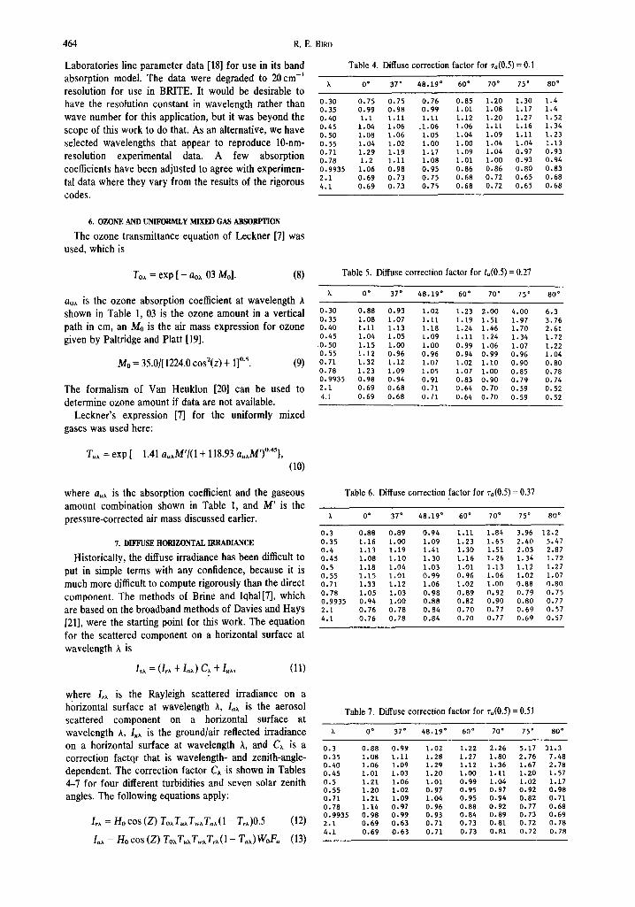
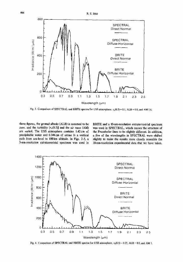
these figures, the ground albedo (ALB) is assumed to be zero, and the turbidity [~,(0.5)] and the air mass (AM) are varied. The USS atmosphere contains 1.42cm of precipitable water and 0.344 cm of ozone in a vertical path from sea-level to 100 km altitude. In Figs. 2-5, a 5-nm-resolution extraterrestrial spectrum was used in

BRITE and a 10-nm-resolution extraterrestrial spectrum was used in SPECTRAL, which causes the structure of the Fraunhofer lines to be slightly different. In addition, a few of the wavelengths in SPECTRAL were shifted slightly to make the results more closely resemble the 10-nm-resolution experimental data that we have taken.

1400

SPECTRAL 1200 Direct Normal

~" 1000 SPECTRAL Diffuse Horizontal

E 800

._~ c 600 Direct Normal "(:3 ~ l . . . . . . . .

-- 400 ,,A BRITE Diffuse Horizontal

200

0 , l , , , l , t , I , J , , . I I ~

0,3 0.5 0.7 0.9 1.1 1.3 1.5 1.7 1.9 2.1 2.3 2.5

Wavelength (pm)

Fig. 4. Comparison of SPECTRAL and BRITE spectra for USS atmosphere, ~(0 .5 ) = 0.27, A L B = 0.0, and A M l.


E

0 C

5 m

1000

800

600

400

200

% I



BRITE Direct Normal

BRITE Diffuse Horizontal

L , 0 0.3 0.5 0.7 0.9 1.1 1.3 1.5 1.7 1.9 2.1 2.3 2.5

Wavelength (pm)

Fig. 5. Comparison of SPECTRAL and BRITE spectra for USS atmosphere, ~'a(0.5) = 0.27, ALB = 0.0, and AM 2.

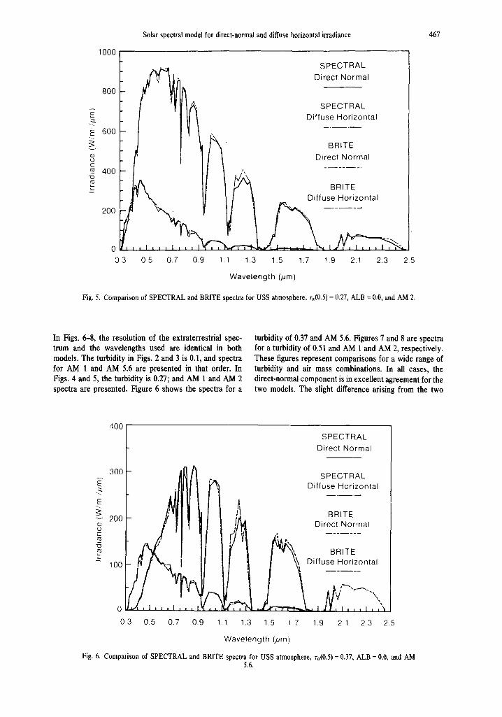
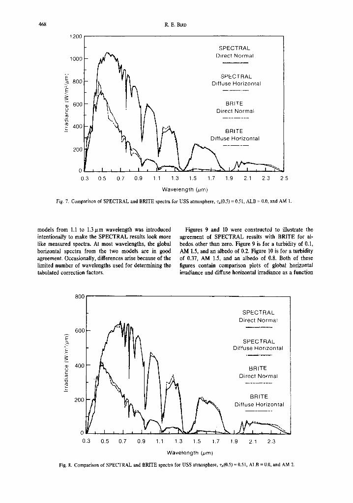
In Figs. 6--8, the resolution of the extraterrestrial spectrum and the wavelengths used are identical in both models. The turbidity in Figs. 2 and 3 is 0.1, and spectra for AM 1 and AM 5.6 are presented in that order. In Figs. 4 and 5, the turbidity is 0.27; and AM 1 and AM 2 spectra are presented. Figure 6 shows the spectra for a

turbidity of 0.37 and AM 5.6. Figures 7 and 8 are spectra for a turbidity of 0.51 and AM 1 and AM 2, respectively. These figures represent comparisons for a wide range of turbidity and air mass combinations. In all cases, the direct-normal component is in excellent agreement for the two models. The slight difference arising from the two

E

{.3 C C~

-5 2

400

300

200

100

i 0

O3 0.5 0.7

l 0.9


7 I

i i


n I t

• ". BRITE /¢~ Direct Normal

FVI I ~ \ BRITE , ,,~ [ ~ Diffuse Horizonta,

/ / ^t, /-" . . . . ,

1.1 1.3 1.5 1.7 19 21 2.3 2.5

Wavelength (pm)

Fig. 6. Comparison of SPECTRAL and BRITE spectra for USS atmosphere, ~'a(0.5) = 0.37, ALB = 0,0, and AM 5.6.

468 R.E. BiRD

1200

1000

a. 800 E

a~ 600 C

5 ~ 4OO

200

o

0.3 2.3 2.5

SPECTRAL ~ j ~ Direct Normal

'~'~[~ V ~ DiffuBR/:Ez°nta'

0.5 0.7 0.9 1.1 1.3 1.5 1.7 1.9 2.1 Wavelength (pro)

Fig. 7. Comparison of SPECTRAL and BRITE spectra for USS atmosphere, za(0.5) = 0.51, ALB = 0.0, and AM 1.

models from 1.1 to 1.3/zm wavelength was introduced intentionally to make the SPECTRAL results look more like measured spectra. At most wavelengths, the global horizontal spectra from the two models are in good agreement. Occasionally, differences arise because of the limited number of wavelengths used for determining the tabulated correction factors.

Figures 9 and 10 were constructed to illustrate the agreement of SPECTRAL results with BRITE for al- bedos other than zero. Figure 9 is for a turbidity of 0.1, AM 1.5, and an albedo of 0.2. Figure 10 is for a turbidity of 0.37, AM 1.5, and an albedo of 0.8. Both of these figures contain comparison plots of global horizontal irradiance and diffuse horizontal irradiance as a function

8OO


600 E SPECTRAL

Diffuse Horizontal

400 BRITE ~ Direct Normal

BRITE 2OO t l ~ l " ~ DiffuseH°riz°ntal

0 I ~ ~ 0.3 0.5 0.7 0.9 1.1 1.3 1.5 1.7 1.9 2.1 2.3

Wavelength (pro)

Fig. 8. Comparison of SPECTRAL and BRITE spectra for USS atmosphere, ~a(0.5) = 0.51, ALB = 0.0, and AM 2.


2000

1800

1600

1400

E 1200

1000 Q) O C

800

'- 600

400

200

0

0.3

SPECTRAL Global Horizontal


BRITE Global Horizontal

BRITE Diffuse Horizontal

0.5 0.7 0.9 1.1 1.3 1.5 1.7 1.9 2.1 2.3 2.5 2.7

I

2.9

Wavelength (pm)

Fig. 9. Comparison of SPECTRAL and BRITE spectra for USS atmosphere, ra(0.5) = 0.I, ALB = 0.2, and AM 1.5.

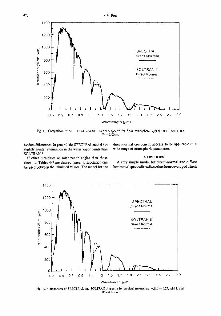
of wavelength. Results from the two models agree well. To illustrate the agreement for different amounts of water vapor, a final comparison is shown in Figs. 11 and 12. The comparison is made between SPECTRAL and SOLTRAN 5 for direct-normal irradiance. The Subarctic Winter (SAW) atmospheric model was used to generate

Fig. 11 where 0.42cm of precipitable water is present. The tropical atmospheric model with 4.12 cm of precipitable water was used for Fig. 12. Note that the SOLTRAN 5 results were generated every 100cm -~ with 20-cm L resolution absorption coefficients. The variable wavelength resolution and spacing causes some of the

SPECTRAL Global Horizontal

1800 [.

1600

1400 F

12OO

1000

800

600

400

200

0 0.3

~~ ~ SPECTRAL - t ~ . Diffuse Horizontal

~ It~ ~ BRITE -o ~- I~..~. Y [ r ~ Global Horizontal

/ ~ , BRITE ~ . " , ~ , ~ ~ ' ~ , / . , ~ Diff use Horizontal

, I , I , I V , ~ , ~ ~ I , ~ ' N ~ I ~ ' 1 " ~ I ~ I

0.5 0.7 0.9 1.1 1.3 1.5 1.7 1.9 2.1 2.3 2.5 2.7 2.9

Wavelength (/am)

Fig. 10. Comparison of SPECTRAL and BRITE spectra for USS atmosphere, ra(0.5) = 0.37, ALB = 0.8, and AM 1.5.

470 R.E. Bled

1400

1200

1000 E

E ~ 800

c 600

~ •

400

200

0 i I i I I , ~

0.3 0.5 0.7 2.7 2.9

| I i I w i i ~ 1 ~ e ~l L i

0.9 1.1 1.3 1.5 1.7 1.9 2.1 2.3 2.5

W a v e l e n g t h (pm)

Fig. 11. Comparison of SPECTRAL and SOLTRAN 5 spectra for SAW atmosphere, ra(0.5)=0.27, AM 1 and W = 0.42 cm.

evident differences. In general, the SPECTRAL model has slightly greater attenuation in the water vapor bands than SOLTRAN 5.

If other turbidities or solar zenith angles than those shown in Tables 4-7 are desired, linear interpolation can be used between the tabulated values. The model for the

direct-normal component appears to be applicable to a wide range of atmospheric parameters.

9. CONCLUSION A very simple model for direct-normal and diffuse

horizontal spectralirradiance has been developed which

1 4 0 0

1200

1000 E

E ~ 800

c 600 5

- 400

200

S P E C T R A L

Di rect Norma l

! S O L T R A N 5 Direct Normal

0 i I , I z I ~ I J ~ " ~ ' ~ ' ~ , , - J , I l

0.3 0.5 0.7 0.9 1.1 1.3 1.5 1.7 1.9 2.1 2.3 2.5 2.7 2.9

Wave leng th (pm)

Fig. 12. Comparison of SPECTRAL and SOLTRAN 5 spectra for tropical atmosphere, za(0.5) = 0.27, AM 1, and W = 4.12 cm.


produces results that agree very well with data from rigorous codes. The model is simple enough that it

should be suitable for anyone desiring spectral data, and it requires a very small computing capability. The spectrum resulting from this model was designed to represent a 10-nm-resolution spectrum, and data are given at 122 points between 0.3 and 4.0 p,m wavelength. The model is limited in the diffuse component to horizontal calculations only. This model is only as accurate as the BRITE and SOLTRAN 5 radiative transfer codes, however, which are currently believed to be -+ 5% on the direct normal and -+ 15 per cent on the diffuse horizontal.

REFERENCES 1. J. V. Dave, Extensive data sets of the diffuse radiation in

realistic atmospheric models with aerosols and common ab- sorbing gases. Solar Energy 21, 361 (1978).

2. R. E. Bird, Terrestrial solar spectral modeling. Solar Cells 7, 107, 1983.

3. R. E. Bird, R. L. Hulstrom and L. J. Lewis, Terrestrial solar spectral data sets. Solar Energy 30, 563 (1983).

4. P. Moon, Proposed standard solar radiation curves for engineering use. J. Franklin Inst 230, 583 (1940).

5. A. P. Thomas and M. P. Thekaekara, Experimental and theoretical studies on solar energy for energy conversion, Int. U.S. Programs Solar Flux (Edited by K. W. Boer), Vol. 1, p. 338 (1976).

6. B. Leckner, The spectral distribution of solar radiation at the Earth's surface-elements of a model. Solar Energy 29, 143 (1978).

7. D. T. Brine and M. Iqbal, Solar spectral diffuse irradiance under cloudless skies. The Renewable Challenge: (Edited by B. H. Glenn and W. A. Kolar) Vol. 2. p. 1271 (1982).

8. H. Neckel and D. Labs, Improved data of solar spectral irradiance from 0.33 to 1.25/tm. Solar Phys. 74, 231 (1981).

9. R. E. Bird, R. L. Hulstrom, A. W. Kliman and H. 13. Eldering, Solar spectral measurements in the terrestrial environment. Appl. Opt. 21, 1430 (1982).

10. R. Pendorf, Tables of the refractive index for standard air

and the rayleigh scattering coefficients. L Opt. Soc. Am. 47, 176 (1957).

11. F. X. Kneizys, E. P. Shettle, W. O. Gallery, J. H. Chetwynd, Jr., L. W. Abreu, J. E. A. Selby, R. W. Fenn and R. A. McClatchey, Atmospheric Transmittance/Radiance: Com- puter Code LOWTRAN 5, Tech. Rep. AFGL-TR-80-O067, U.S. Air Force Geophysics Laboratory, Bedford, Mas- sachusetts (1980).

12. F. Kasten, A new table and approximate formula for relative optical air mass. Arch. Meteorol. Geophys. Bioclimatol., Ser B14, 206 (1966).

13. M. Kerker, The Scattering of Light and Other Electromag- netic Radiation, p. 31. Academic Press, New York (1969).

14. A. T. Young, On rayleigh scattering optical depth of the atmosphere. J. Appl. Metrology 20, 328 (1981).

15. E. P. Shettle and R..W. Fenn, Models of the atmospheric aerosol and their optical properties. Proc. Advisory Group for Aerospace Research and Development Conf. No. 183, Optical Propagation in the Atmosphere, pp. 2.1-2.16. Presented at the Electromagnetic Wave Propagation Panel Symposium, Lyngby, Denmark (27-31 October 1975).

16. A. Angstrom, Techniques of determining the turbidity of the atmosphere. Tellus 13, 214 (1961).

17. M. D. King and B. M. Herman, Determination of the ground albedo and the index of absorption of atmospheric parti- culates by remote sensing--Part I: Theory. J. of the Atmos- pheric Sci. 36, 163 (1979).

18. L. S. Rothman, Update of the AFGL atmospheric absorption line parameters compilation. Appl. Opt. 17, 3517 (1978).

19. G. W. Paltridge and C. M. R. Platt, Radiative Processes in Meteorology and Climatology, p. 92. Elsevier, New York (1976).

20. T. K. Van Heuklon, Estimating atmospheric ozones for solar radiation models. Solar Energy 22, 63 (1979).

21. J. A. Davies and J. E. Hay, Calculation of solar radiation incident on a horizontal surface. Proc. 1st Canadian Solar Radiation Data Workshop (Edited by J. Hay and T. K. Won), p. 32 (1980).

22. R. A. McClatchey, R. W. Fenn, J. E. A. Selby, F. E. Volz and J. S. Garing, Optical Properties of the Atmosphere (3rd Edition), Tech. Rep. AFGL-72--0497, U.S. Air Force Cam- bridge Research Laboratories (1972).

a simple, solar spectral model for direct-normal and diffuse horizontal irradiance

Documents