a simple second-order reduced bias’ tail index estimator

This article was downloaded by: [Duke University Libraries]On: 07 October 2014, At: 15:23Publisher: Taylor & FrancisInforma Ltd Registered in England and Wales Registered Number: 1072954 Registeredoffice: Mortimer House, 37-41 Mortimer Street, London W1T 3JH, UK

Journal of Statistical Computation andSimulationPublication details, including instructions for authors andsubscription information:http://www.tandfonline.com/loi/gscs20

A simple second-order reduced bias’tail index estimatorM. Ivette Gomes a & Dinis Pestana aa Universidade de Lisboa , FCUL (DEIO) and CEAUL, Lisboa,PortugalPublished online: 21 May 2007.

To cite this article: M. Ivette Gomes & Dinis Pestana (2007) A simple second-order reduced bias’tail index estimator, Journal of Statistical Computation and Simulation, 77:6, 487-502, DOI:10.1080/10629360500282239

To link to this article: http://dx.doi.org/10.1080/10629360500282239

PLEASE SCROLL DOWN FOR ARTICLE

Taylor & Francis makes every effort to ensure the accuracy of all the information (the“Content”) contained in the publications on our platform. However, Taylor & Francis,our agents, and our licensors make no representations or warranties whatsoever as tothe accuracy, completeness, or suitability for any purpose of the Content. Any opinionsand views expressed in this publication are the opinions and views of the authors,and are not the views of or endorsed by Taylor & Francis. The accuracy of the Contentshould not be relied upon and should be independently verified with primary sourcesof information. Taylor and Francis shall not be liable for any losses, actions, claims,proceedings, demands, costs, expenses, damages, and other liabilities whatsoever orhowsoever caused arising directly or indirectly in connection with, in relation to or arisingout of the use of the Content.

This article may be used for research, teaching, and private study purposes. Anysubstantial or systematic reproduction, redistribution, reselling, loan, sub-licensing,systematic supply, or distribution in any form to anyone is expressly forbidden. Terms &Conditions of access and use can be found at http://www.tandfonline.com/page/terms-and-conditions

http://www.tandfonline.com/loi/gscs20

http://www.tandfonline.com/action/showCitFormats?doi=10.1080/10629360500282239

http://dx.doi.org/10.1080/10629360500282239

http://www.tandfonline.com/page/terms-and-conditions

http://www.tandfonline.com/page/terms-and-conditions

Journal of Statistical Computation and SimulationVol. 77, No. 6, June 2007, 487–504

A simple second-order reduced bias’ tail index estimator

M. IVETTE GOMES* and DINIS PESTANA

Universidade de Lisboa, FCUL (DEIO) and CEAUL, Lisboa, Portugal

(Received 19 January 2005; in final form 28 April 2005)

In this article, we are interested in the direct estimation of the dominant component of the bias of aclassical tail index estimator, such as the Hill estimator, used here for illustration of the procedure. Suchan estimated bias is then directly removed from the original estimator. The second-order parameters inthe bias are based on a number of top order statistics, larger than the one we should use for the estimationof the tail index γ , so that there is no change in the asymptotic variance of the new reduced bias’ tailindex estimator, which is kept equal to the asymptotic variance of the classical original one, contrarilyto what happens with most of the reduced bias’ estimators available in the literature. The asymptoticdistributional behaviour of the proposed estimators of γ is derived, under a second-order framework,and their finite sample properties are also obtained through Monte Carlo simulation techniques.

Keywords: Statistics of extremes; Semi-parametric estimation; Bias estimation; Heavy tails; Hill’sestimator

AMS 2000 Subject Classification: Primary: 62G32; Secondary: 65C05

1. Introduction and the new tail index estimators

In statistics of extremes, the tail index γ is one of the primary parameters of extreme events,and it plays a relevant role, either implicit or explicit, in other extreme events’parameters suchas high quantiles and return periods of high levels. We may have γ ∈ R and the heaviness of thetail function F := 1 − F , with F the underlying model, increases with γ . Here we shall con-sider the particular case γ > 0, i.e. we shall work with heavy-tailed models. This type ofmodels has revealed to be quite useful in most diversified fields such as computer sci-ence, biostatistics, telecommunication networks, insurance, finance and economics. Then,F must be a regularly varying function with a negative index of regular variation equalto {−1/γ }, γ > 0. Equivalently, the quantile function U(t) = F←(1 − 1/t), t ≥ 1, withF←(u) = inf{y: F(y) ≥ u}, is of regular variation with index γ , i.e. for every x > 0,

limt→∞

F (tx)

F (t)= x−1/γ ⇐⇒ lim

t→∞U(tx)

U(t)= xγ . (1)

*Corresponding author. DEIO, Faculdade de Ciencias de Lisboa, Cidade Universitária, Campo Grande, 1749-016Lisboa, Portugal. Email: [email protected]

Journal of Statistical Computation and SimulationISSN 0094-9655 print/ISSN 1563-5163 online © 2007 Taylor & Francis

http://www.tandf.co.uk/journalsDOI: 10.1080/10629360500282239

Dow

nloa

ded

by [

Duk

e U

nive

rsity

Lib

rari

es]

at 1

5:23

07

Oct

ober

201

4

488 M. I. Gomes and D. Pestana

Then, we are in the domain of attraction for maxima of an extreme value distribution function(df),

EVγ (x) = exp(−(1 + γ x)−1/γ ), 1 + γ x ≥ 0, with γ > 0,

and we denote this fact by F ∈ DM(EVγ ), γ > 0. Indeed, F ∈ DM(EVγ ), γ > 0, if andonly if equation (1) holds true.

The second-order parameter ρ (≤0) rules the rate of convergence in the first-order condition(1) and is the non-positive parameter appearing in the limiting relation

limt→∞

ln U(tx) − ln U(t) − γ ln x

A(t)= xρ − 1

ρ, (2)

which we assume to hold for every x > 0 and where |A(t)| must then be of regular variationwith index ρ [1]. We shall assume, everywhere in the article, that ρ < 0.

For intermediate k, i.e. a sequence of integers k = kn, 1 ≤ k < n such that

k = kn −→ ∞, kn = o(n), as n −→ ∞, (3)

we shall consider, as basic statistics, the scaled log spacings,

Wi := i{ln Xn−i+1:n − ln Xn−i:n}, 1 ≤ i ≤ k < n, (4)

where Xi:n denotes, as usual, the ith ascending order statistic (os), 1 ≤ i ≤ n, associated to arandom sample (X1, X2, . . . , Xn).

As Xi:nd= U(Yi:n), where {Yi} denotes a sequence of unit Pareto random variables (rvs), i.e.

P(Y ≤ y) = 1 − 1/y, y ≥ 1, and as ln Y1:id= E1:i

d= Ei/i, where {Ei} denotes a sequence ofindependent standard exponential rvs, we may write, whenever we are under the first-orderframework in equation (1),

Wid= i

(ln

U(Yn−i+1:n)U(Yn−i:n)

)d= i

(ln

U(Yn−i:nY1:i )U(Yn−i:n)

)d≈ γEi, 1 ≤ i ≤ k,

i.e. the Wis, 1 ≤ i ≤ k, are approximately independent and exponential with mean value γ .Then, the Hill estimator of γ [2],

Hn(k) := 1

k

k∑i=1

Wi, (5)

is consistent for the estimation of γ whenever equation (1) holds and k is intermediate, i.e.equation (3) holds.

Under the second-order framework in equation (2), the asymptotic distributional represen-tation

Hn(k)d= γ + γ√

kZk + A(n/k)

1 − ρ+ op

(A

(n

k

))(6)

holds true [3], where Zk = √k (

∑ki=1 Ei/k − 1) is an asymptotically standard normal rv.

Then,√

k(Hn(k) − γ ) is asymptotically normal with variance equal to γ 2 and mean valueequal to λ/(1 − ρ) whenever

√kA(n/k) → λ, finite, as n → ∞.

Dow

nloa

ded

by [

Duk

e U

nive

rsity

Lib

rari

es]

at 1

5:23

07

Oct

ober

201

4

Simple second-order reduced bias’ tail index estimator 489

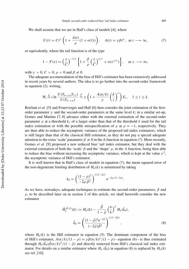
We shall assume that we are in Hall’s class of models [4], where

U(t) = Ctγ(

1 + A(t)

ρ(1 + o(1))

), A(t) = γβtρ, as t −→ ∞, (7)

or equivalently, where the tail function is of the type

1 − F(x) =( x

C

)−1/γ{

1 + β

ρ

( x

C

)ρ/γ + o(xρ/γ )

}, as x −→ ∞,

with γ > 0, C > 0, ρ < 0 and β �= 0.The adequate accommodation of the bias of Hill’s estimator has been extensively addressed

in recent years by several authors. The idea is to go further into the second-order frameworkin equation (2), writing,

Wid= i ln

U(Yn−i:nY1:i )U(Yn−i:n)

d≈ γ

(1 + A(n/k)

γ

(k

i

)ρ)Ei, 1 ≤ i ≤ k.

Beirlant et al. [5] and Feuerverger and Hall [6] then consider the joint estimation of the first-order parameter γ and the second-order parameters at the same level k; in a similar set-up,Gomes and Martins [7, 8] advance either with the external estimation of the second-orderparameter ρ at a threshold k1 of a larger order than that of the threshold k used for the tailindex estimation or with the possible misspecification of ρ at ρ = −1, respectively. Theyare then able to reduce the asymptotic variance of the proposed tail index estimators, whichis still larger than that of the classical Hill estimator, as they do not pay a special adequateattention to the extra ‘scale’ parameter β �= 0 in the A function in equation (7). More recently,Gomes et al. [9] proposed a new reduced bias’ tail index estimator, but they deal with theexternal estimation of both the ‘scale’ β and the ‘shape’ ρ, in the A function, being then ableto reduce the bias without increasing the asymptotic variance, which is kept at the value γ 2,the asymptotic variance of Hill’s estimator.

It is well known that in Hall’s class of models in equation (7), the mean squared error ofthe non-degenerate limiting distribution of Hn(k) is minimized by taking

k0 =(

(1 − ρ)2

−2ρ β2

)1/(1−2ρ)

n−2ρ/(1−2ρ).

As we have, nowadays, adequate techniques to estimate the second-order parameters, β andρ, to be described later on in section 2 of this article, we shall herewith consider the newestimator

H (β,ρ)n (k) := Hn(k) − β

1 − ρ

(n

k

)ρ

Hn(k0),

k0 =(

(1 − ρ)2n−2ρ

(−2ρ)β2

)1/(1−2ρ)

, (8)

where Hn(k) is the Hill estimator in equation (5). The dominant component of the biasof Hill’s estimator, A(n/k)/(1 − ρ) = γβ(n/k)ρ/(1 − ρ) – equation (6) – is thus estimatedthrough Hn(k0)β(n/k)ρ/(1 − ρ) and directly removed from Hill’s classical tail index esti-mator. For details on a similar estimator where Hn (k0) in equation (8) is replaced by Hn(k)

see ref. [10].

Dow

nloa

ded

by [

Duk

e U

nive

rsity

Lib

rari

es]

at 1

5:23

07

Oct

ober

201

4


Remark 1.1 Note that heavy-tailed models have compulsory an infinite right endpoint.When-ever the left endpoint of the model is negative or −∞, the sample size n should be replacedby n+, the number of positive observations in the sample. Some authors prefer, however, toinduce a deterministic shift in the data, to work only with positive values.

In section 2 of this article, and as mentioned earlier, we shall briefly review the estimationof the two second-order parameters β and ρ. Section 3 is devoted to the derivation of the

asymptotic behaviour of the estimator H(β,ρ)n (k) in equation (8), whenever we estimate β and

ρ at a value k1 > k, k being the value used for the tail index estimation. Finally, in section 4,and through the use of Monte Carlo simulation techniques, we shall exhibit the performanceof the new estimators in equation (8), comparatively to the classical Hill estimator. We alsopresent some of the characteristics of the second-order parameters’ estimators and draw someoverall conclusions in the final subsection of the article.

2. Second-order parameter estimation

As our estimator of β depends on the estimation of ρ, we shall first address the estimation ofthe shape second-order parameter.

2.1 The estimation of the shape second-order parameter ρ

Nowadays, we have two general classes of ρ-estimators, which work reasonably well inpractice, the ones introduced by Gomes et al. [11] and FragaAlves et al. [12]. We shall considerhere particular members of the class of estimators of the second-order parameter ρ proposedby Fraga Alves et al. [12]. Under adequate general conditions, they are semi-parametric,asymptotically normal estimators of ρ, whenever ρ < 0, with highly stable sample paths asfunctions of k, the number of top oss used for a certain τ = τu. Such a class of estimatorshas been first parameterized in a tuning parameter τ > 0, which may be straightforwardlygeneralized to the case τ ∈ R, as done in ref. [13], and may be defined as

ρτ (k) ≡ ρ(τ )n (k) := −

∣∣∣∣3(T (τ)n (k) − 1)

T(τ)n (k) − 3

∣∣∣∣ , (9)

where

T (τ)n (k) :=

⎧⎪⎪⎪⎨⎪⎪⎪⎩

(M(1)n (k))τ − (M(2)

n (k)/2)τ/2

(M(2)n (k)/2)τ/2 − (M

(3)n (k)/6)τ/3

if τ �= 0,

ln(M(1)n (k)) − (1/2) ln(M(2)

n (k)/2)

(1/2) ln(M(2)n (k)/2) − (1/3) ln(M

(3)n (k)/6)

if τ = 0,

with

M(j)n (k) := 1

k

k∑i=1

{ln

Xn−i+1:nXn−k:n

}j

, j ≥ 1 [M(1)n ≡ Hn in (5)].

The statistics ρ(τ )n (k) in equation (9) converge towards ρ, for every τ ∈ R, whenever the

second-order condition (2) holds and k is such that k → ∞, k = o(n) and√

k A(n/k) → ∞,as n → ∞.

We shall here summarize a particular case of the results proved by Fraga Alves et al. [12].

Dow

nloa

ded

by [

Duk

e U

nive

rsity

Lib

rari

es]

at 1

5:23

07

Oct

ober

201

4


PROPOSITION 2.1 Under the second-order framework in equation (2) with ρ < 0, ifequation (3) holds and if

√kA(n/k) → ∞, as n → ∞, the statistic ρ(τ )

n (k) in equation (9)converges in probability towards ρ, as n → ∞, for any real τ . Moreover, we have ρ(τ )

n (k) −ρ = Op(1/(

√kA(n/k))), for adequate choices of k or τ .

Remark 2.1 The theoretical and simulated results by Fraga Alves et al. [12], together withthe use of these estimators in the Generalized Jackknife statistics of Gomes et al. [14], asdone by Gomes and Martins [7] and Gomes et al. [9, 15] have led us to advise in practice theconsideration of the tuning parameters τ = 0 for the region ρ ∈ [−1, 0) and τ = 1 for theregion ρ ∈ (−∞, −1), together with the intermediate level

k1 = min

(n − 1,

[2n

ln2 n

])(10)

(not chosen in any optimal way, but in the conditions of Proposition 2.1), with the obviousnotation ln2 n = ln ln n. We however advise practitioners not to choose blindly the value of τ

in equation (9). It is sensible to draw a few sample paths of ρ(τ )n (k) in equation (9), as functions

of k, electing the value of τ = τu which provides the highest stability for large k, by means ofany stability criterion – see ref. [16].

Remark 2.2 When we consider the level k1 in equation (10), together with ρu = ρTu(k1), we

are able to practically remove the bias of the ρ-estimator in equation (9) and to guarantee that{ρu − ρ} is of the order of 1/(

√k1A(n/k1)) = O((ln2 n)(1−2ρ)/2/

√n).

Remark 2.3 Consequently, for any level k, (ρu − ρ) ln(n/k) = op(1), and then√kA(n/k)(ρu − ρ) ln(n/k) = op(1) whenever

√kA(n/k) → λ, finite.

2.2 Estimation of the second-order parameter β

Here we have considered the estimator of β obtained by Gomes and Martins [7] and based onthe scaled log-spacings Wi in equation (4), 1 ≤ i ≤ k. Let ρ denote any of the estimators inequation (9) computed at the level k1 in equation (10). The β-estimator is given by

βρ (k) :=(

k

n

)ρ

((1/k)

∑ki=1(i/k)−ρ

)((1/k)

∑ki=1 Wi

)−

((1/k)

∑ki=1(i/k)−ρWi

)((1/k)

∑ki=1(i/k)−ρ

)((1/k)

∑ki=1(i/k)−ρWi

)−

((1/k)

∑ki=1(i/k)−2ρWi

) ,

(11)

and as the numerator in the above written fraction goes to zero and the denominator convergesin probability towards

γ

(1 − ρ)2− γ

1 − 2ρ= γρ2

(1 − ρ)2(1 − 2ρ),

βρ(k) is asymptotically equivalent to

− (1 − ρ)2(1 − 2ρ)

γρ2

(k

n

)p{(

1

k

k∑i=1

(i

k

)−ρ) (

1

k

k∑i=1

Wi

)− 1

k

k∑i=1

(i

k

)−ρ

Wi

}.

In Gomes and Martins [7], and later in Gomes et al. [9], the following result has beenproved.

Dow

nloa

ded

by [

Duk

e U

nive

rsity

Lib

rari

es]

at 1

5:23

07

Oct

ober

201

4


PROPOSITION 2.2 If the second-order condition (2) holds, with A(t) = γβtρ , ρ < 0, if k = kn

is a sequence of intermediate positive integers, i.e. (3) holds, and if√

k A(n/k) → ∞, asn → ∞, then βρ (k) in (11) is consistent for the estimation of β, whenever ρ is consistent forthe estimation of ρ. If we consider βρ(k)(k), then

βρ(k)(k) − β ∼ −β ln(n/k)(ρ(k) − ρ). (12)

Remark 2.4 Note that when we consider the level k1 in (10), and βu ≡ βρu(k1), with ρu the

estimator in (9), computed also at the same level k1 and associated to the tuning param-eter τu, the use of equation (12) enables us to guarantee that βu − β is of the order ofln(n/k1)/(

√k1A(n/k1)) = O(ln3 n(ln2 n)(1−2ρ)/2/

√n).

3. Asymptotic behaviour of the estimators

Let us first assume that only the tail index parameter γ is unknown.

THEOREM 3.1 Under the second-order framework in (2), further assuming that A(t) may bechosen as in (7) and for levels k such that (3) holds, we get, for H

(β,ρ)n (k) in (8), an asymptotic

distributional representation of the type

H (β,ρ)n (k)

d= γ + γ√kZk + R

(γ )

k , with R(γ )

k = op(A(n/k)), (13)

where Zk = √k

(∑ki=1 Ei/k − 1

)is an asymptotically standard normal rv. Consequently,√

k (H(β,ρ)n (k) − γ ) is asymptotically normal with variance equal to γ 2 and with a null mean

value not only when√

k A(n/k) → 0, but also when√

k A(n/k) → λ �= 0, finite, as n → ∞.

Proof This result comes from the fact that if all parameters are known, apart from the tailindex γ , we get from (6),

H (β,ρ)n (k)

d= γ + γ√kZk + A(n/k)

1 − ρ(1 + op(1)) − A(n/k)

(1 − ρ)(1 + op(1))

d= γ + γ√kZk + op(A(n/k)),

i.e. equation (13) holds. The remaining of the theorem then follows straightforwardly. �

Let us assume now that we estimate both β and ρ externally at the level k1 in equation (10).We may state the following.

THEOREM 3.2 Under the conditions of Theorem 3.1, let us consider the tail index estimators

H(β,ρ)n (k) in (8), for estimators ρ and β in (9) and (11), respectively, both computed at a level

k1 that implies ρ − ρ = op(1/ ln n). Then,√

k{H (β,ρ)n (k) − γ } is asymptotically normal with

null mean value, not only when√

k A(n/k) → 0, but also whenever√

k A(n/k) → λ, finite,as n → ∞.

Proof If we estimate consistently β and ρ through the estimators β and ρ in the conditionsof the theorem, we may use Taylor’s expansion series, i.e. the Delta method [17, pp. 240–245],

Dow

nloa

ded

by [

Duk

e U

nive

rsity

Lib

rari

es]

at 1

5:23

07

Oct

ober

201

4


and write,

β

1 − ρ

(n

k

)ρd= β

1 − ρ

(n

k

)ρ + (β − β)1

1 − ρ

(n

k

)ρ

(1 + op(1))

+ β

1 − ρ(ρ − ρ)

(n

k

)ρ(

1

1 − ρ+ ln

(n

k

))(1 + op(1))

d= A(n/k)

γ (1 − ρ)

(1 + β − β

β+ (ρ − ρ) ln

(n

k

))(1 + op(1)).

As β and ρ are consistent for the estimation of β and ρ, respectively, and (ρ − ρ) ln(n/k) =op(1) (see Remark 2.3), the summands related to (β − β) and (ρ − ρ) are both op(A(n/k)).

Moreover, as Hn(k0)d= γ (1 + op(1)),

H β,ρn (k) := Hn(k) − β

1 − ρ

(n

k

)ρ

Hn(k0)

d= γ + γ√kZk + op(A(n/k),

and the results of the theorem follow. �

Remark 3.1 Note that the levels k such that√

k A(n/k) → λ, finite, are suboptimal for thistype of estimators. To go further to the optimal level, we should consider levels k such that√

kA(n/k) → ∞, as n → ∞ and should go further into a third-order framework, as been donein ref. [18], in a probabilistic context and whenever dealing with the penultimate behaviour ofextremes detected by [19], in refs. [11, 12] for the estimation of the second-order parameterρ, and in ref. [15] for the estimation of the tail index γ , through an estimator derived from theone by Caeiro and Gomes [20].

4. Finite sample behaviour of the estimators

We have here implemented a multi-sample Monte Carlo simulation experiment of size 5000 ×10, to obtain the distributional behaviour of the new estimators H

(β,ρ)n in equation (8), based

on the estimators of ρ and β in equations (9) and (11), respectively, all computed at thesame level k1 = min(n − 1, [2n/ ln2 n]), not chosen in any optimal way. For any details onmulti-sample simulation, see Gomes and Oliveira [21]. We use the notation βj = βρj

(k1),

ρj = ρj (k1), j = 0, 1, with ρj (k) and βρ (k) given in equations (9) and (11), respectively.Similar to what has been done in ref. [9], for the reduced bias’ estimator therewith introduced,these estimators of ρ and β have been incorporated in the estimator under study, leading to

H (0)n (k) ≡ H

(β0,ρ0)n (k) and to H (1)

n (k) ≡ H(β1,ρ1)n (k). The simulations show that the tail index

estimators H(j)n (k), with j equal to either 0 or 1, according as |ρ| ≤ 1 or |ρ| > 1, seem to

work quite well, as illustrated in the sequel. Indeed, for all models simulated, the use of H (1)

always enables us to achieve a better performance than the one we get with the Hill estimatorH . In a ‘blind’ way, we may thus advise the choice of H (1). However, H (0) provides muchbetter results than H (1) whenever |ρ|, unknown, is smaller than or equal to 1.

As mentioned before, in Remark 2.1, the different data analysis performed convinced usthat it would be sensible to choose ρ0 whenever the sample path associated with τ = 0 shows

Dow

nloa

ded

by [

Duk

e U

nive

rsity

Lib

rari

es]

at 1

5:23

07

Oct

ober

201

4


a higher stability than the one associated with τ = 1, choosing ρ1 otherwise. We have thenimplemented the simulation of the estimator in equation (8), associated to the following choiceof the ρ-estimator.

(a) For j from k0 = [k1 − 0.05 × n] to k1, k1 given in equation (10), compute ρ0(j) andρ1(j), k0 ≤ j ≤ k1. Find the medians of those samples, denoted χ0 and χ1, respectively.

(b) Compute then

Si :=k1∑

j=k0

(ρi(j) − χi)2, i = 0, 1.

(c) Consider H (01)n (k) ≡ H

(β01,ρ01)n (k),

ρ01 :={

ρ0 if S0 < S1

ρ1 otherwiseand β0,1 := βρ01(k1), (14)

with H(β,ρ)n , k1 and βρ (k) given in equation (8), (10) and (11), respectively.

Unfortunately, and against our intuition, this criterion leads to the choice of ρ0 too manytimes, for models with |ρ| > 1 and unless n is large, this leads partially to the disappearanceof the nice properties of H (1)

n in this region of ρ-values, as illustrated, later on, in figure 4. Theheuristic criterion has thus been slightly misleading, and we have decided to proceed with theimplementation of another criterion for the choice of the ρ-estimator, playing again with ρ0

and ρ1. The criterion is similar to the aforementioned one, but (c) is replaced by

(c′) Consider ˜H(01)n (k) ≡ H

(β01,ρ01)n (k),

ρ01 :={

ρ0 if S0 < S1 and |ρ0| < 1

ρ1 otherwiseand β01 := βρ01(k1), (15)

again with H(β,ρ)n , k1 and βρ (k) given in equations (8), (10) and (11), respectively.

The use of this last criterion leads practically to no changes whenever we work with modelswith |ρ| ≤ 1, different from the Fréchet model. For the Fréchet model, ρ1 is chosen most ofthe times. However, for models with |ρ| > 1, we highly increase the percentage of times ρ1 isused, being then led to a result similar to the one we obtain with H (1)

n . The use of the criterionleading to equation (15) seems thus to be one of the best compromises between the choice ofeither ρ0 or ρ1. In practice, we think however advisable to draw a few sample paths of ρτ (k)

in equation (9), for different values of τ , and choose the tuning parameter τu as suggested inthe final part of Remark 2.1.

4.1 Mean values and mean squared error patterns of the tail index estimators

In figures 1 and 2, we show the simulated patterns of mean values E[•] and mean squared

errors MSE[•] of H (0)n ≡ H

(β0,ρ0)n in equation (8) and of the Hill estimator H in equation (5),

for samples of size n = 1000 from two models with γ = 1 and ρ = −1, the Fréchet andthe Burr. The Fréchet(γ ) df is F(x) = exp{−x−1/γ }, x ≥ 0, γ > 0, and the Burr(γ, ρ) dfis F(x) = 1 − (1 + x−ρ/γ )1/ρ , x ≥ 0, γ > 0, ρ < 0. For comparison, we also picture theanalogue behaviour of the rv Hn ≡ H

(β,ρ)n . The discrepancy between the behaviour of the

Dow

nloa

ded

by [

Duk

e U

nive

rsity

Lib

rari

es]

at 1

5:23

07

Oct

ober

201

4


0.9

1.0

1.1

0 200 400 600 800 200 400 600 8000.00

0.01

0.02

0.03

0

Hn

k k

MSE •[ ]E •[ ]

Hn( , )β ρ

H Hn n( ) ( )0 01≅

Hn( , )β ρ

H Hn n( ) ( )0 01≅

H Hn n( ) ( )˜1 01≅

Hn

H Hn n( ) ( )˜1 01≅

Figure 1. Simulated mean values (left) and mean squared errors (right) of H(0)n , H

(1)n , H

(01)n , ˜H(01)

n , the associatedrv Hn and the Hill estimator H , for samples of size n = 1000 from a Fréchet parent with γ = 1 (ρ = −1).

estimators and of the associated rv, for some of the models, suggests that some improvementin the estimation of second-order parameters β and ρ may still be welcome. The mean valuesand mean squared errors of the estimators are based on the first replicate, with 5000 runs.Note that the use of ρ01 leads to patterns which overlap the ones pictured for H (0)

n . The samehappens if we use ρ01 in a Burr model. However, if we use ρ01 in the Fréchet model, we get aresult closer to the one we get when we use ρ1.

In table 1, we present the percentage of times we use ρ0 in a Fréchet model and in a Burrmodel with ρ = −1, under the criteria leading to equations (14) and (15).

k

Hn

k

MSE •[ ]E •[ ]

Hn( , )β ρ

Hn( )0

Hn( , )β ρ

Hn( )0

Hn

0.8

1.0

1.2

0.00

0.02

0.04

0 200 400 600 0 200 400 600

Figure 2. Simulated mean values (left) and mean squared errors (right) of H(0)n (almost overlaping with H

(01)n and

˜H(01)n ), the associated rv Hn = H

(β,ρ)n and the Hill estimator H for samples of size n = 1000 from a Burr parent with

(γ, ρ) = (1, −1).

Table 1. Percentage of times ρ0 is used, under the criteria leading to (14)/(15).

n 100 200 500 1000 2000 5000 10,000

Fréchet 93.3/41.0 89.2/24.7 86.1/7.5 86.2/1.4 88.6/1.0 88.1/2.9 89.7/2.0Burr (ρ = −1) 91.7/89.6 90.6/90.3 93.0/93.0 96.3/96.3 97.3/97.3 95.4/95.3 96.0/95.8

Dow

nloa

ded

by [

Duk

e U

nive

rsity

Lib

rari

es]

at 1

5:23

07

Oct

ober

201

4


0.5

1.0

1.5

0 200 4000.00

0.02

0.04

0.06

0.08

0.10

0 200 400

Hn

k k

MSE •[ ]E •[ ]

Hn( , )β ρ

Hn( )0

Hn( , )β ρ

Hn

Hn( )0

Figure 3. Simulated mean values (left) and mean squared errors (right) of H(0)n (almost overlaping with H

(01)n and

˜H(01)n ), the associated rv Hn ≡ H

(β,ρ)n and the Hill estimator H , for samples of size n = 1000 from a Burr parent

with (γ, ρ) = (1, −0.5).

Note that although for the Fréchet model, there is a big decrease in the percentage of timesρ0 is used, when we move from the criterion leading to equation (14) towards the one leadingto equation (15), the decrease is not significant when we are working with a Burr model, withρ = −1.

Figures 3 and 4 are equivalent to figures 1 and 2, but for Burr parents with ρ = −0.5 andρ = −2. In figure 4, we also picture the mean value and mean squared error of H (0,1)

n , still a

bit far away from H (1)n . The estimates ˜H(0,1)

n (k) almost overlap with H (1)n (k).

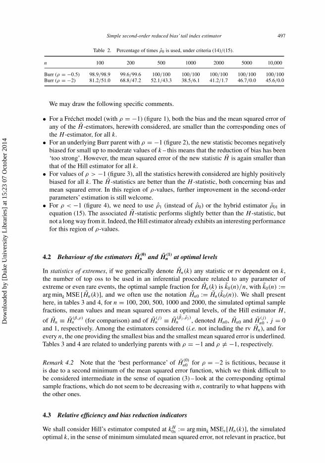
Table 2 is equivalent to table 1, but for Burr models with ρ = −0.5 and ρ = −2. Note thatfor ρ = −2, we have a big decrease in the percentage of times ρ0 is used. This is the reason

why ˜H(01)n is quite close to H (1)

n for n ≥ 1000.

Remark 4.1 For a Burr model and for any of the estimators considered, BIAS/γ and MSE/γ 2

are independent of γ , for every ρ.

k

Hn

k

MSE •[ ]E •[ ]

Hn( , )β ρ

Hn( )1

Hn( , )β ρ

Hn( )01

Hn( )01

Hn( )1

Hn

0.9

1.0

1.1

0 200 400 600 800 200 400 600 8000.00

0.01

0.02

0.03

0

Figure 4. Simulated mean values (left) and mean squared errors (right) of H(1)n (almost overlaping with ˜H(01)

n ),H

(01)n , the associated rv Hn ≡ H

(β,ρ)n and the Hill estimator H , for samples of size n = 1000 from a Burr parent with

(γ, ρ) = (1, −2).

Dow

nloa

ded

by [

Duk

e U

nive

rsity

Lib

rari

es]

at 1

5:23

07

Oct

ober

201

4


Table 2. Percentage of times ρ0 is used, under criteria (14)/(15).

n 100 200 500 1000 2000 5000 10,000

Burr (ρ = −0.5) 98.9/98.9 99.6/99.6 100/100 100/100 100/100 100/100 100/100Burr (ρ = −2) 81.2/51.0 68.8/47.2 52.1/43.3 38.5/6.1 41.2/1.7 46.7/0.0 45.6/0.0

We may draw the following specific comments.

• For a Fréchet model (with ρ = −1) (figure 1), both the bias and the mean squared error ofany of the H -estimators, herewith considered, are smaller than the corresponding ones ofthe H -estimator, for all k.

• For an underlying Burr parent with ρ = −1 (figure 2), the new statistic becomes negativelybiased for small up to moderate values of k – this means that the reduction of bias has been‘too strong’. However, the mean squared error of the new statistic H is again smaller thanthat of the Hill estimator for all k.

• For values of ρ > −1 (figure 3), all the statistics herewith considered are highly positivelybiased for all k. The H -statistics are better than the H -statistic, both concerning bias andmean squared error. In this region of ρ-values, further improvement in the second-orderparameters’ estimation is still welcome.

• For ρ < −1 (figure 4), we need to use ρ1 (instead of ρ0) or the hybrid estimator ρ01 inequation (15). The associated H -statistic performs slightly better than the H -statistic, butnot a long way from it. Indeed, the Hill estimator already exhibits an interesting performancefor this region of ρ-values.

4.2 Behaviour of the estimators H(0)n and H

(1)n at optimal levels

In statistics of extremes, if we generically denote Hn(k) any statistic or rv dependent on k,the number of top oss to be used in an inferential procedure related to any parameter ofextreme or even rare events, the optimal sample fraction for Hn(k) is k0(n)/n, with k0(n) :=arg mink MSE [Hn(k)], and we often use the notation Hn0 := Hn(k0(n)). We shall presenthere, in tables 3 and 4, for n = 100, 200, 500, 1000 and 2000, the simulated optimal samplefractions, mean values and mean squared errors at optimal levels, of the Hill estimator H ,

of Hn ≡ H(β,ρ)n (for comparison) and of H

(j)n ≡ H

(βj ,ρj )n , denoted Hn0, Hn0 and H

(j)

n0 , j = 0and 1, respectively. Among the estimators considered (i.e. not including the rv Hn), and forevery n, the one providing the smallest bias and the smallest mean squared error is underlined.Tables 3 and 4 are related to underlying parents with ρ = −1 and ρ �= −1, respectively.

Remark 4.2 Note that the ‘best performance’ of H(0)n0 for ρ = −2 is fictitious, because it

is due to a second minimum of the mean squared error function, which we think difficult tobe considered intermediate in the sense of equation (3) – look at the corresponding optimalsample fractions, which do not seem to be decreasing with n, contrarily to what happens withthe other ones.

4.3 Relative efficiency and bias reduction indicators

We shall consider Hill’s estimator computed at kH0s := arg mink MSEs[Hn(k)], the simulated

optimal k, in the sense of minimum simulated mean squared error, not relevant in practice, but

Dow

nloa

ded

by [

Duk

e U

nive

rsity

Lib

rari

es]

at 1

5:23

07

Oct

ober

201

4


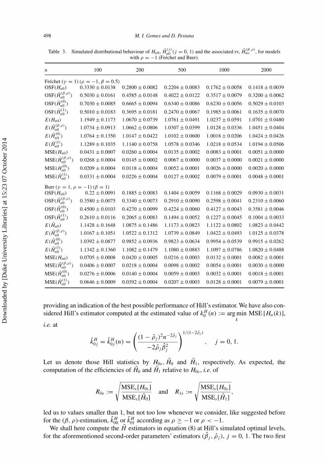
Table 3. Simulated distributional behaviour of Hn0, H(j)n0 (j = 0, 1) and the associated rv, H

(β,ρ)no , for models

with ρ = −1 (Fréchet and Burr).

n 100 200 500 1000 2000

Fréchet (γ = 1) (ρ = −1, β = 0.5)

OSF(Hn0) 0.3330 ± 0.0138 0.2800 ± 0.0082 0.2204 ± 0.0083 0.1762 ± 0.0058 0.1418 ± 0.0039

OSF(H(β,ρ)n0 ) 0.5030 ± 0.0161 0.4585 ± 0.0148 0.4022 ± 0.0122 0.3517 ± 0.0079 0.3200 ± 0.0062

OSF(H(0)n0 ) 0.7030 ± 0.0085 0.6665 ± 0.0094 0.6340 ± 0.0086 0.6230 ± 0.0056 0.5029 ± 0.0103

OSF(H(1)n0 ) 0.5010 ± 0.0183 0.3695 ± 0.0181 0.2470 ± 0.0067 0.1985 ± 0.0061 0.1635 ± 0.0070

E(Hn0) 1.1949 ± 0.1173 1.0670 ± 0.0739 1.0761 ± 0.0491 1.0237 ± 0.0591 1.0701 ± 0.0480

E(H(β,ρ)n0 ) 1.0734 ± 0.0913 1.0662 ± 0.0806 1.0307 ± 0.0399 1.0128 ± 0.0336 1.0451 ± 0.0404

E(H(0)n0 ) 1.0764 ± 0.1350 1.0147 ± 0.0422 1.0102 ± 0.0600 1.0018 ± 0.0206 1.0424 ± 0.0426

E(H(1)n0 ) 1.1289 ± 0.1035 1.1140 ± 0.0758 1.0578 ± 0.0346 1.0218 ± 0.0534 1.0194 ± 0.0506

MSE(Hn0) 0.0431 ± 0.0007 0.0260 ± 0.0004 0.0135 ± 0.0002 0.0083 ± 0.0001 0.0051 ± 0.0000

MSE(H(β,ρ)n0 ) 0.0268 ± 0.0004 0.0145 ± 0.0002 0.0067 ± 0.0000 0.0037 ± 0.0000 0.0021 ± 0.0000

MSE(H(0)n0 ) 0.0209 ± 0.0004 0.0118 ± 0.0004 0.0052 ± 0.0001 0.0026 ± 0.0000 0.0020 ± 0.0000

MSE(H(1)n0 ) 0.0331 ± 0.0004 0.0226 ± 0.0004 0.0127 ± 0.0002 0.0079 ± 0.0001 0.0048 ± 0.0001

Burr (γ = 1, ρ = −1) (β = 1)OSF(Hn0) 0.22 ± 0.0091 0.1885 ± 0.0083 0.1404 ± 0.0059 0.1168 ± 0.0029 0.0930 ± 0.0031

OSF(H(β,ρ)n0 ) 0.3580 ± 0.0075 0.3340 ± 0.0073 0.2910 ± 0.0090 0.2598 ± 0.0041 0.2310 ± 0.0060

OSF(H(0)n0 ) 0.4500 ± 0.0103 0.4270 ± 0.0099 0.4224 ± 0.0060 0.4127 ± 0.0043 0.3581 ± 0.0046

OSF(H(1)n0 ) 0.2610 ± 0.0116 0.2065 ± 0.0083 0.1494 ± 0.0052 0.1227 ± 0.0045 0.1004 ± 0.0033

E(Hn0) 1.1428 ± 0.1648 1.0875 ± 0.1486 1.1173 ± 0.0823 1.1122 ± 0.0802 1.0823 ± 0.0442

E(H(β,ρ)n0 ) 1.0167 ± 0.1051 1.0522 ± 0.1312 1.0739 ± 0.0849 1.0422 ± 0.0493 1.0125 ± 0.0378

E(H(0)n0 ) 1.0392 ± 0.0877 0.9852 ± 0.0936 0.9823 ± 0.0634 0.9954 ± 0.0539 0.9915 ± 0.0262

E(H(1)n0 ) 1.1342 ± 0.1360 1.1082 ± 0.1479 1.1080 ± 0.0883 1.1097 ± 0.0786 1.0820 ± 0.0488

MSE(Hn0) 0.0705 ± 0.0008 0.0420 ± 0.0005 0.0216 ± 0.0003 0.0132 ± 0.0001 0.0082 ± 0.0001

MSE(H(β,ρ)n0 ) 0.0406 ± 0.0007 0.0218 ± 0.0004 0.0098 ± 0.0002 0.0054 ± 0.0001 0.0030 ± 0.0000

MSE(H(0)n0 ) 0.0276 ± 0.0006 0.0140 ± 0.0004 0.0059 ± 0.0003 0.0032 ± 0.0001 0.0018 ± 0.0001

MSE(H(1)n0 ) 0.0646 ± 0.0009 0.0392 ± 0.0004 0.0207 ± 0.0003 0.0128 ± 0.0001 0.0079 ± 0.0001

providing an indication of the best possible performance of Hill’s estimator. We have also con-sidered Hill’s estimator computed at the estimated value of kH

0 (n) := arg mink

MSE [Hn(k)],i.e. at

kH0j = kH

0j (n) =(

(1 − ρj )2n−2ρj

−2ρj β2j

)1/(1−2ρj )

, j = 0, 1.

Let us denote those Hill statistics by H0s , H0 and H1, respectively. As expected, thecomputation of the efficiencies of H0 and H1 relative to H0s , i.e. of

R0s :=√

MSEs[H0s]MSEs[H0]

and R1s :=√

MSEs[H0s]MSEs[H1]

,

led us to values smaller than 1, but not too low whenever we consider, like suggested beforefor the (β, ρ)-estimation, kH

00 or kH01 according as ρ ≥ −1 or ρ < −1.

We shall here compute the H estimators in equation (8) at Hill’s simulated optimal levels,for the aforementioned second-order parameters’ estimators (βj , ρj ), j = 0, 1. The two first

Dow

nloa

ded

by [

Duk

e U

nive

rsity

Lib

rari

es]

at 1

5:23

07

Oct

ober

201

4


Table 4. Simulated distributional behaviour of Hn0, H(j)n0 (j = 0, 1) and the associated rv, H

(β,ρ)n0 , for Burr

parents with γ = 1 and ρ �= −1 (β = 1).

n 100 200 500 1000 2000

ρ = −0.5OSF(Hn0) 0.1010 ± 0.0073 0.0780 ± 0.0039 0.0520 ± 0.0034 0.0384 ± 0.0013 0.0300 ± 0.0013

OSF(H(β,ρ)n0 ) 0.1900 ± 0.0060 0.1555 ± 0.0070 0.1222 ± 0.0055 0.1007 ± 0.0024 0.0839 ± 0.0026

OSF(H(0)n0 ) 0.2040 ± 0.0061 0.1545 ± 0.0061 0.1040 ± 0.0022 0.0739 ± 0.0028 0.0497 ± 0.0030

OSF(H(1)n0 ) 0.1070 ± 0.0060 0.0785 ± 0.0039 0.0524 ± 0.0034 0.0384 ± 0.0013 0.0300 ± 0.0013

E(Hn0) 1.4258 ± 0.2467 1.1877 ± 0.2112 1.2578 ± 0.1554 1.1986 ± 0.1107 1.1380 ± 0.0783

E(H(β,ρ)n0 ) 1.1571 ± 0.1920 1.0996 ± 0.1751 1.1715 ± 0.0917 1.1165 ± 0.0859 1.0941 ± 0.0480

E(H(0)n0 ) 1.2842 ± 0.1667 1.1778 ± 0.1568 1.2162 ± 0.1158 1.1619 ± 0.0840 1.1733 ± 0.0445

E(H(1)n0 ) 1.4272 ± 0.2348 1.1799 ± 0.2105 1.2534 ± 0.1526 1.1982 ± 0.1107 1.1375 ± 0.0783

MSE(Hn0) 0.2286 ± 0.0030 0.1450 ± 0.0026 0.0834 ± 0.0012 0.0557 ± 0.0011 0.0374 ± 0.0006

MSE(H(β,ρ)n0 ) 0.1162 ± 0.0021 0.0659 ± 0.0012 0.0318 ± 0.0005 0.0188 ± 0.0002 0.0112 ± 0.0001

MSE(H(0)n0 ) 0.1135 ± 0.0026 0.0754 ± 0.0020 0.0455 ± 0.0008 0.0320 ± 0.0007 0.0233 ± 0.0004

MSE(H(1)n0 ) 0.2246 ± 0.0029 0.1436 ± 0.0026 0.0830 ± 0.0012 0.0556 ± 0.0011 0.0373 ± 0.0006

ρ = −2OSF(Hn0) 0.4150 ± 0.0179 0.3620 ± 0.0165 0.3218 ± 0.0106 0.2902 ± 0.0086 0.2493 ± 0.0114

OSF(H(β,ρ)n0 ) 0.5860 ± 0.0176 0.5585 ± 0.0186 0.5142 ± 0.0176 0.4865 ± 0.0119 0.4554 ± 0.0170

OSF(H(0)n0 ) 0.7850 ± 0.0071 0.8000 ± 0.0038 0.8156 ± 0.0025 0.8250 ± 0.0012 0.7712 ± 0.0009

OSF(H(1)n0 ) 0.5710 ± 0.0155 0.5080 ± 0.0272 0.4492 ± 0.0200 0.3938 ± 0.0197 0.3578 ± 0.0097

E(Hn0) 1.0894 ± 0.0856 1.0931 ± 0.0886 1.0426 ± 0.0650 1.0341 ± 0.0497 1.0352 ± 0.0366

E(H(β,ρ)n0 ) 1.0520 ± 0.0543 1.0588 ± 0.0601 1.0506 ± 0.0424 1.0252 ± 0.0363 1.0203 ± 0.0274

E(H(0)n0 ) 1.0029 ± 0.0662 0.9928 ± 0.0583 1.0018 ± 0.0576 0.9944 ± 0.0499 1.0229 ± 0.0172

E(H(E)n0 ) 1.0600 ± 0.0594 1.0793 ± 0.0593 1.0504 ± 0.0562 1.0245 ± 0.0431 1.0261 ± 0.0315

MSE(Hn0) 0.0291 ± 0.0012 0.0161 ± 0.0006 0.0076 ± 0.0003 0.0044 ± 0.0001 0.0025 ± 0.0001

MSE(H(β,ρ)n0 ) 0.0205 ± 0.0007 0.0105 ± 0.0003 0.0045 ± 0.0001 0.0024 ± 0.0001 0.0013 ± 0.0000

MSE(H(0)n0 ) 0.0179 ± 0.0006 0.0099 ± 0.0002 0.0045 ± 0.0001 0.0027 ± 0.0001 0.0010 ± 0.0000

MSE(H(1)n0 ) 0.0212 ± 0.0008 0.0119 ± 0.0004 0.0056 ± 0.0002 0.0032 ± 0.0001 0.0019 ± 0.0001

indicators are related to the behaviour of the new estimators at Hill’s optimal simulated level,i.e. for j = 0 and 1, we have simulated

R(j)

0s :=√

MSEs[Hn(kH0s )]

MSEs[H (j)n (kH

0s )]and B

(j)

0s :=∣∣∣∣∣ Es[Hn(k

H0s ) − γ ]

Es[H (j)n (kH

0s ) − γ ]

∣∣∣∣∣ .We have also simulated these same indicators, but computed at the level kH

0j . They will be

denoted R(j)

0s and B(j)

0s , j = 0, 1. Finally, we have simulated two extra indicators, relatedto the comparison of mean squared errors and bias of the new estimators with those of theHill’s estimators, when all the estimators are considered at their optimal levels. The two extrasimulated indicators are, again for j = 0, 1,

R(j)

0s :=√

MSEs[Hn0]MSEs[H (j)

n0 ] and B(j)s :=

∣∣∣∣∣ Es[Hn0 − γ ]Es[H (j)

n0 − γ ]

∣∣∣∣∣ .Remark 4.3 Note that an indicator higher than one means a better performance than the Hillestimator. Consequently, the higher these indicators are, the better the new estimators perform,comparatively to the Hill estimator.

Dow

nloa

ded

by [

Duk

e U

nive

rsity

Lib

rari

es]

at 1

5:23

07

Oct

ober

201

4


Table 5. REFF indicators.

n

100 200 500 1000 2000

Fréchet parent: ρ = −1, γ = 11.04/1.06/1.44 1.06/1.08/1.48 1.08/1.10/1.62 1.09/1.12/1.80 1.08/1.14/1.601.06/1.30/1.14 1.04/1.26/1.07 1.03/1.22/1.03 1.02/1.20/1.02 1.02/1.18/1.03

Burr parent: ρ = −0.5, γ = 11.22/1.71/1.42 1.19/1.66/1.39 1.20/1.60/1.35 1.20/1.56/1.32 1.17/1.50/1.271.01/1.16/1.01 1.00/1.12/1.01 1.00/1.09/1.00 1.00/1.07/1.00 1.00/1.07/1.00

Burr parent: ρ = −1, γ = 11.25/1.31/1.60 1.26/1.23/1.73 1.18/1.14/1.92 1.13/1.09/2.05 1.14/1.10/2.151.04/1.28/1.04 1.03/1.24/1.04 1.02/1.19/1.02 1.01/1.16/1.02 1.02/1.17/1.02

Burr parent: ρ = −2, γ = 10.82/0.89/1.28 0.71/0.86/1.27 0.55/0.84/1.30 0.45/0.83/1.27 0.58/0.85/1.561.07/1.23/1.17 1.07/1.23/1.16 1.08/1.23/1.17 1.08/1.23/1.17 1.05/1.20/1.14

In tables 5 and 6, we present the REFF and the BRI indicators, respectively. For each modeland for each value of n, the first and second rows are related to j = 0 and j = 1, respectively.Each entry has three numbers: in table 5, the numbers are R

(j)

0s /R(j)

0s /R(j)

0s ; similarly, in table 6,the numbers are B

(j)

0s /B(j)

0s /B(j)

0s .

Remark 4.4 Note that in tables 5 and 6, the unique values smaller than 1 appear when, forρ = −2, we consider H (0)

n (k) and compute this H -estimator at Hill’s optimal levels (eithersimulated or estimated). All other entries are greater than one.

4.4 Behaviour of the second-order parameters’ estimators

In figures 5–8, we picture the mean values and mean squared errors patterns of the β andthe ρ-estimators, β0(k), β1(k), ρ0(k) and ρ1(k), for Fréchet(γ = 1) and Burr(γ = 1, ρ)parents with ρ = −0.5, −1 and −2, respectively. Note that for not too large values of n,like the one considered here (n = 1000), the sample paths of ρτ in equation (9) are highly

Table 6. BRI indicators.

n

100 200 500 1000 2000

Fréchet parent: ρ = −1, γ = 13.02/1.73/4.32 4.84/2.64/4.25 6.35/3.84/5.58 9.21/4.86/7.50 10.16/21.18/3.491.61/1.87/1.06 1.32/1.55/1.01 1.16/1.37/1.04 1.10/1.29/0.98 1.14/1.31/0.99

Burr parent: ρ = −0.5, γ = 12.13/2.18/1.35 1.97/2.05/1.31 1.83/1.92/1.23 1.71/1.82/1.21 1.60/1.72/1.241.02/1.169/0.99 1.01/1.13/1.01 1.01/1.09/1.00 1.00/1.07/1.00 1.00/1.07/1.00

Burr parent: ρ = −1, γ = 13.48/3.19/10.76 2.51/2.23/89.31 1.57/1.44/29.49 1.29/1.16/786.96 1.76/1.53/38.141.17/1.36/1.00 1.12/1.28/1.02 1.08/1.21/1.00 1.05/1.17/1.00 1.07/1.186/1.00

Burr parent: ρ = −2, γ = 10.50/0.16/6.21 0.40/0.09/12.25 0.27/0.04/14.42 0.21/0.03/43.13 0.29/0.05/409.283.32/3.18/1.39 2.63/2.72/1.24 2.45/2.49/1.19 2.33/2.39/1.22 2.18/2.33/1.07

Dow

nloa

ded

by [

Duk

e U

nive

rsity

Lib

rari

es]

at 1

5:23

07

Oct

ober

201

4


−3

−4

−2

−1

0

1

2

400 600 800 1000

0.0

0.5

1.0

1.5

2.0

2.5

3.0

400 600 800 1000

k

k

MSE •[ ]E •[ ]

ρ0

ρ1

β1β0

ρ0

ρ1

β1

β0

ρ = −1

β = 0 5.

Figure 5. Simulated mean values (left) and mean squared errors (right) of the second-order parameters’ estimators,for samples of size n = 1000 from a Fréchet parent with γ = 1 (β = 0.5, ρ = −1).

−2

−1

0

1

2

400 600 800 1000

0.00

0.20

0.40

0.60

400 600 800 1000

k

k

MSE •[ ]E •[ ]

ρ0ρ1

β1β0

ρ0

ρ1

β1

β0

ρ = −0 5.

β =1

Figure 6. Simulated mean values (left) and mean squared errors (right) of the second-order parameters’ estimators,for samples of size n = 1000 from a Burr parent with (γ, ρ) = (1, −0.5)(β = 1).

−4

−3

−2

−1

0

1

2

400 600 800 1000

0.0

0.2

0.4

0.6

0.8

1.0

400 600 800 1000

ρ = −1

β =1

k

k

MSE •[ ]E •[ ]

ρ0

ρ1

β1

β0

ρ0

ρ1β1

β0

Figure 7. Simulated mean values (left) and mean squared errors (right) of the second-order parameters’ estimators,for samples of size n = 1000 from a Burr parent with (γ, ρ) = (1, −1)(β = 1).

Dow

nloa

ded

by [

Duk

e U

nive

rsity

Lib

rari

es]

at 1

5:23

07

Oct

ober

201

4


−4

−3

−2

−1

0

1

2

400 600 800 1000

0.0

0.2

0.4

0.6

0.8

1.0

400 600 800 1000

ρ = −2

β =1

k

E •[ ]

ρ0

ρ1

β1

β0

k

MSE •[ ]

ρ0

ρ1

β1

β0

Figure 8. Simulated mean values (left) and mean squared errors (right) of the second order parameters’ estimators,for samples of size n = 1000 from a Burr parent with (γ, ρ) = (1, −2)(β = 1).

volatile for not too large values of k and some of the models. This is the reason why wehave pictured large values of k only. Such a volatility justifies also the choice of k1 inequation (10).

In table 7, we present the mean values and standard deviations of the different ρ-estimatorsconsidered in this study: ρτ ≡ ρτ (k1) for τ = 0 and 1, with ρτ (k) and k1 given in equations (9)and (10), respectively, ρ01 in equation (14) and ρ01 in equation (15).

Table 7. Mean values/standard deviations of the different ρ-estimators.

n ρ0 ρ1 ρ01 ρ01

Fréchet parent: ρ = −1, γ = 1100 −1.189/0.485 −2.258/0.765 −1.283/0.690 −1.895/1.059200 −1.224/0.368 −2.395/0.622 −1.377/0.670 −2.153/0.893500 −1.216/0.223 −2.469/0.388 −1.413/0.622 −2.387/0.5471000 −1.199/0.140 −2.494/0.243 −1.397/0.581 −2.478/0.2992000 −1.268/0.123 −2.258/0.274 −1.399/0.489 −2.249/0.289

Burr parent: ρ = −0.5, γ = 1100 −0.753/0.036 −2.077/0.146 −0.769/0.155 −0.769/0.156200 −0.754/0.020 −2.138/0.097 −0.760/0.092 −0.760/0.092500 −0.752/0.010 −2.190/0.059 −0.752/0.022 −0.752/0.0221000 −0.749/0.007 −2.217/0.042 −0.749/0.010 −0.749/0.0102000 −0.757/0.006 −2.004/0.037 −0.757/0.009 −0.757/0.009

Burr parent: ρ = −1, γ = 1100 −0.820/0.086 −2.130/0.183 −0.935/0.414 −0.965/0.476200 −0.809/0.047 −2.182/0.107 −0.942/0.430 −0.947/0.440500 −0.796/0.026 −2.226/0.057 −0.897/0.378 −0.897/0.3781000 −0.787/0.019 −2.247/0.038 −0.841/0.281 −0.841/0.2812000 −0.842/0.017 −2.074/0.036 −0.876/0.213 −0.876/0.213

Burr parent: ρ = −2, γ = 1100 −1.051/0.304 −2.383/0.504 −1.325/0.742 −1.748/0.970200 −1.011/0.192 −2.412/0.321 −1.464/0.734 −1.776/0.868500 −0.954/0.097 −2.409/0.137 −1.659/0.729 −1.791/0.5831000 −0.918/0.065 −2.403/0.074 −1.838/0.721 −2.395/0.3292000 −1.149/0.045 −2.416/0.060 −1.909/0.689 −2.396/0.243

Dow

nloa

ded

by [

Duk

e U

nive

rsity

Lib

rari

es]

at 1

5:23

07

Oct

ober

201

4


4.5 Some overall conclusions

• The use of these new statistics enables us to gain in mean value stability, reached now alonga wider range of k-values. This property of the mean values gives an obvious indicationabout the sample paths’ behaviour of these new estimators, as, under a different scale, thesample paths are identical to the corresponding mean values.

• In addition, with these new statistics we do gain a lot concerning mean squared error at theoptimal level. More important than that: the mean squared error of the new estimator inequation (8) is smaller than that of the the Hill estimator in equation (5) for every k, providedwe estimate adequately the second-order parameters. Consequently, the H -statistic is notan alternative to Hill’s estimator, for intermediate large values of k, like most of the reducedbias’ tail index estimators available in the literature: it is a substitute of Hill’s estimator,performing better than the Hill estimator for all k.

• Indeed, the main advantage of these estimators lies on the fact that we may estimate β andρ adequately and easily, through the estimators β and ρ herewith suggested, so that theMSE of the new estimator is smaller than the MSE of Hill’s estimator for all k, even when|ρ| > 1, a region where it has been difficult to find alternatives for the Hill estimator, andthis happens together with a higher stability of the sample paths around the target value γ .

Acknowledgements

This research was partially supported by FCT/POCTI and POCI/FEDER.

References

[1] Geluk, J. and de Haan, L., 1987, Regular Variation, Extensions and Tauberian Theorems. CWI Tract 40, Centerfor Mathematics and Computer Science, Amsterdam, The Netherlands.

[2] Hill, B.M., 1975, A simple general approach to inference about the tail of a distribution. Annals of Statistics, 3,1163–1174.

[3] de Haan, L. and Peng, L., 1998, Comparison of tail index estimators. Statistica Neerlandica, 52, 60–70.[4] Hall, P. and Welsh, A.H., 1985, Adaptive estimates of parameters of regular variation. Annals of Statistics, 13,

331–341.[5] Beirlant, J., Dierckx, G., Goegebeur, Y. and Matthys, G., 1999, Tail index estimation and an exponential

regression model. Extremes, 2, 177–200.[6] Feuerverger, A. and Hall, P., 1999, Estimating a tail exponent by modelling departure from a Pareto distribution.

Annals of Statistics, 27, 760–781.[7] Gomes, M.I. and Martins, M.J., 2002, ‘Asymptotically unbiased’ estimators of the tail index based on external

estimation of the second order parameter. Extremes, 5(1), 5–31.[8] Gomes, M.I. and Martins, M.J., 2004, Bias reduction and explicit semiparametric estimation of the tail index.

Journal of Statistical Planning and Inference, 124, 361–378.[9] Gomes, M.I., de Haan, L. and Henriques, L., 2004, Tail index estimation through accommodation of bias in the

weighted log-excesses. Notas e Comunicações C.E.A.U.L. 14/2004. Submitted for publication.[10] Caeiro, F., Gomes, M.I. and Pestana, D., 2005, Direct reduction of bias of the classical Hill estimator. Rev Stat,

3(2), 113–136.[11] Gomes, M.I., de Haan, L. and Peng, L., 2002, Semi-parametric estimation of the second order parameter –

asymptotic and finite sample behaviour. Extremes, 5(4), 387–414.[12] Fraga Alves, M.I., Gomes, M.I. and de Haan, L., 2003, A new class of semiparametric estimators of the second

order parameter. Portugaliae Mathematica, 60(1), 193–213.[13] Caeiro, F. and Gomes, M.I., 2004, A new class of estimators of a ‘scale’ second order parameter. Notas e

Comunicções CEAUL 20/2004. Submitted for publication.[14] Gomes, M.I., Martins, M.J. and Neves, M., 2000, Alternatives to a semiparametric estimator of parameters of

rare events – the Jackknife methodology. Extremes, 3(3), 207–229.[15] Gomes, M.I., Caeiro, F. and Figueiredo, F., 2004, Bias reduction of a tail index estimator through an external

estimation of the second order parameter. Statistics, 38(6), 497–510.[16] Gomes, M.I. and Figueiredo, F., 2003, Bias reduction in risk modelling: semiparametric quantile estimation.

Accepted at Test.[17] Casella, G. and Berger, R.L., 2002, Statistical Inference (2nd edn) (Pacific Grove, USA: Duxbury).

Dow

nloa

ded

by [

Duk

e U

nive

rsity

Lib

rari

es]

at 1

5:23

07

Oct

ober

201

4


[18] Gomes, M.I. and de Haan, L., 1999, Approximation by penultimate extreme value distributions. Extremes, 2(1),71–85.

[19] Gomes, M.I., 1984, Penultimate limiting forms in extreme value theory. Annals of Institute of StatisticalMathematics, 36(1), 71–85.

[20] Caeiro, F. and Gomes, M.I., 2002, A class of ‘asymptotically unbiased’ semiparametric estimators of the tailindex. Test, 11(2), 345–364.

[21] Gomes, M.I. and Oliveira, O., 2001, The bootstrap methodology in statistical extremes – choice of the optimalsample fraction. Extremes, 4(4), 331–358.

Dow

nloa

ded

by [

Duk

e U

nive

rsity

Lib

rari

es]

at 1

5:23

07

Oct

ober

201

4

a simple second-order reduced bias’ tail index estimator

Documents