a simple muscle model

8/7/2019 A Simple Muscle Model

http://slidepdf.com/reader/full/a-simple-muscle-model 1/18

Supplementary documents for “Computational Neurobiology of Reaching and Pointing”, by R. Shadmehr and S. P. Wise

A SIMPLE MUSCLE MODEL

Muscle produces two kinds of force, active and passive, which sum to compose a muscle’s total force. A muscle’scontractile elements provide its active force through the actin and myosin “ratcheting” mechanism. Noncontractile

elements contribute its passive force. Technically, a muscle’s passive element has properties most correctly termed

elastic, but it can be modeled more simply as a spring. Because this spring-like element attaches in series with thecontractile element, you can think of the force that the contractile element produces as an active force transmitted to

the skeleton via a series elastic element. Muscles, however, have another elastic element, as well, called a parallelelastic element, that also contributes to its passive force.

Figure 1. A simple shock absorber (a damper). The force on the piston cannot change the position of the

piston instantaneously. It must push against a liquid that has a certain viscosity. The relation between the

force on the piston and the speed with which the position of the piston changes is governed by the following

equation: Force (or tension) equals viscosity times speed xbT = .

In 1922, A. V. Hill (see Hill, 1970) first noted that activated muscles produce more force when heldisometrically (i.e., at a length fixed) than when they shorten. When muscles shorten, they appear to waste some of

their active force in overcoming an inherent resistance. This resistance could not result from the series elastic

element because it resists lengthening not shortening. So Hill thought of this resistance as another kind of passiveforce in the muscle. He found that the faster a muscle shortens, the less total force it produces. Assuming a constant

active force, Hill concluded that the faster shortening leads to a larger resistive force.

Hill drew an analogy between the resistive force a shock absorber. A piston in a viscous fluid exemplifies

a simple shock absorber, also known as a damper (Figure 1). If you push on its piston, a shock absorber will resistby a tension T (equivalent to a force) that depends on the viscosity b of the fluid in its cavity. The faster you try to

push the piston, the stronger the fluid resists. For a given speed x , the force that you need to move the piston is

xbT = . To account for the fact that muscle produces less force when it shortens, Hill proposed that this viscous

element lies in parallel with the contractile element. Accordingly, this component can be called a parallel elastic

element.

To investigate the properties of this viscous element, Hill and his colleagues performed a simpleexperiment. They attached a muscle to a bar that pivoted around a point (Figure 2A). One end of the bar had a

catch mechanism that they could release at any time. A basket held a weight on the other end of the bar. When Hill




released the catch, this weight would pull on the muscle by a force T . The experiment began with the catch in place

and the muscle stimulated maximally. The stimulation resulted in the production of force T o in the muscle. Because

the muscle pulled on a bar that could not move, the force that the muscle produced did not change the muscle’s

length.

A

E

D

C

B

Figure 2. Development of a mathematical muscle model . In this experiment, a muscle is being stimulated

when the catch is released. Because there is less weight in the basket than the force that is being produced

by the muscle, the muscle shortens rapidly by an amount and then gradually by a different amount. From

the changes in the length and tension in the muscle, a muscle model is produced. [From T.A. McMahon

(1984)].

At this point, the experimenters released the catch. Note, in Figure 2C, how the length of the muscle

suddenly shortened and, in Figure 2B, how the force dropped to T from T o. After this rapid phase of shortening,

Figure 2C shows how the muscle continued to shorten, but now gradually. The fact that the muscle immediately

shortened by amount ∆x1 and reduced its force from T o to T suggests that something in the muscle acted like a

spring. If you put tension on a spring by pulling it, then suddenly release it, the spring will rapidly shorten. This

spring is the series elastic (SE) element referred to above and its stiffness is K SE in Figure 2E. Recall that stiffnessrelates changes in force (or tension) to changes in length:

L

F K

∆∆

= (1)

After the immediate change in muscle length and force, a slow, gradual change in length developed (Figure

2C), without any change in force (Figure 2B). Whereas a part of the muscle’s mechanism changed length rapidly inresponse to the force change, another part did not change as quickly—as if a “shock absorber” acted on the “spring,”

slowing its response to the force change. The parallel elastic (PE) element, referred to above, represents this second

passive element in the muscle, and its stiffness is K PE in Figure 2E.The muscle’s viscosity, the parallel elastic element and the series elastic element compose the passive

components of an elementary model muscle. In Figure 2, the length of the series elastic element is x1 and the length

of the parallel elastic element is x2. Note that this is a model of a muscle: it does not imply that the variouscomponents have this physical arrangement within a muscle. Further, the viscous component of muscle tension

results from mechanisms very different from the mechanical damper depicted in Figure 1. Mathematically,

however, the characteristics of the muscle accord reasonably well with this depiction. You might think of the model




as a simile. In the model, like in a muscle, when the tension in the system suddenly decreases, the series elastic

element responds immediately, but the parallel elastic element responds gradually because of its viscous component.

The muscle’s active component contributes the final piece of the mathematical muscle model. This active

force acts against the passive components of the model (and muscles) to produce the final force that acts on the bar

in Figure 2D. Function A indicates the active component in Figure 2E.The model can now describe how the total force produced by the muscle depends on its passive and active

components. Assume that the series elastic element—its most spring-like component—has a resting length*1x and

the parallel elastic spring has a resting length*2x . The same force T develops in both of these elements because the

muscle can have only one force at any given time. Thus,

Because the total length of the muscle must be the sum of the lengths of the series elastic and parallel elastic

elements:

)()( *22

*11

**2

*1

*

21

xxxxxxxxx

xxx

−+−=−⇒+=

+=

you can substitute:

SE SE

SE

PE PE

PE PE

K

T xx

K

T x

AxxbK

T K xxK T

AxbxxK xxK T

=⇒+=

+−+−−=

++−−−=

1

*

11

1

*

2

*

11

*

)()(

)()(

and arrive at a relationship between muscle force and muscle length:

A

K

T xb

K

T K xxK T

SE SE

PE PE +−+−−= )()( *

(2)

When you bring the rate of change of force with respect to time T to the left side of the equation, you have a model

of a typical muscle:

⎟⎟⎠

⎞⎜⎜⎝

⎛ ++−+∆= AT

K

K xbxK

b

K T

SE

PE PE

SE )1(

(3)

Note that in this equation, the active force A, muscle length x, its rate of change x , and force T are all function of

time.

Mathematical model versus real muscles

How well does this model capture the behavior of a real muscle? Figure 3A shows the tension of a frog

gastrocnemius muscle under various conditions. The gastrocnemius is the calf muscle, and somehow the frog’sgastrocnemius became a prototype for skeletal muscles in the early days of motor physiology. Other muscles may

differ in certain details, but the basic principles of striated muscle are highly conserved in evolution. In the

experiment described here, the muscle was stimulated electrically. As Figure 3A shows, the first excitatory inputcaused an initial isometric twitch. Later, during maximal activation, tetanus occurred, which represents the

maximal sustained output that the muscle can produce. During maximal activation, the muscle was stretched

AxbxxK T

xxK T

PE

SE

++−=

−=

2

*

22

*

11

)(

and

)(




(Figure 3B) and held in a fixed, stretched state for about one second, then released. Shortly after release, the

stimulation stopped.

A

B

Figure 3. Muscle force output. A frog’s gastrocnemius muscle produces force as a result of an isometric

twitch, followed by tetanus, followed by a displacement (muscle stretch). A. Muscle tension. B. Muscle

length. [From Inbar and Adams (1976)].

Immediately after the stretch, the muscle’s force level increased rapidly. According to the model, the series

elastic element must have caused this increase because the active component had reached its maximal output prior to

the stretch—recall that the muscle was in tetany. Figure 3 shows that this force increase amounted to 150 g, which,for a change in length of 1.1 cm, means that stiffness:

g/cm 136cm 1.1

g 150==SE

K

After the stretch, the force in the muscle slowly declined to a steady-state value (arrow in Figure 3A). You can

compare the steady-state values of force before and after the stretch and use the change to solve for parameter K PE in

the model. Using Eq. (2), you have:

AxxK K

K T PE

SE

PE +−=+ )()1(

:stretch Before

*

11

AxxK K

K T PE

SE

PE +−=+ )()1(

:stretchAfter *

22

xK K

K T PE

SE

PE ∆=+ )1(∆

:forceinChange




T

x

K K

K K

SE PE

PE SE

∆

∆=

+

g/cm 75=PE K

Thus, the stiffness of the series elastic element exceeds that of the parallel elastic element. However,

stiffness does not completely describe the passive component of the parallel elasticity because it also has viscosity.

Accordingly, your final step is to estimate the viscosity of the parallel elastic element. Consider the conditions after the sudden stretch: the length of the muscle, as shown in Figure 3B, did not change (i.e., 0=x ). Nevertheless, the

force gradually dropped, as shown in Figure 3A (arrow). If you arbitrarily call the time of the sudden muscle stretch

t = 0, then the force in the muscle was:

( ) )(1)(

)0(

t T K

K

b

K AxK

b

K t T

AxK T

SE

PE SE

PE

SE

SE

⎟⎟⎠

⎞⎜⎜⎝

⎛ +−+∆=

+∆=

This statement is a differential equation of the form )()( 21 t T aat T −= , which has a general solution of the form

( )[ ]t acaat T 221 exp/)( −⋅+= , where c is a constant that depends on the initial conditions, e.g., force at time

zero. Solving the differential equation produces

⎥⎦⎤+−⋅⎢

⎣⎡

+∆++

+∆+= )exp()()(

2

t b

K K

K K

xK AK

K K

xK AK t T SE PE

SE PE

SE PE

SE PE

PE SE

Note that in an exponential function of the form ( )τ /exp t − , the time constant τ specifies the time when the

exponential has declined by about 63%. From the muscle force trace of Figure 3A, you might estimate that

23.0=τ sec for the frog’s calf muscle. From this you have

50 g s/cmPE SE

bb

K K τ = ⇒ ≈ ⋅

+

Simulation of passive properties

Now that you have the parameters of the muscle model, you can simulate its behavior and compare the results of

that simulation to empirical data.

Figure 4 shows the results of the simulation. Assume that a muscle is at rest at t = 0 and its length is 1.0 cm. You

simulate pulling on the muscle for 0.05 sec so that its length increases linearly by 1.0 cm over this period. Hold the

muscle at this new length for an additional 0.95 seconds, at which this point you release the muscle and its length

returns to the original 1.0 cm at time 1.05 sec. Using Eq. (3), you can simulate the force produced in this muscle (

Figure 4A). If you increase viscosity, the trace declines slower when the muscle is stretched, and rises slower when

the muscle is released compared to the trace shown in the figure.




Force (g)

0.5 1 1.5 2

-50

50

100

0 Time (sec)

Length (cm) 2

A

B

1

0

0.05

Figure 4. Simulation of the mathematic muscle model. A. Output of Eq. (3) for a stretch of 1.0 cm, and

then release at t = 1.0 sec. B. Shows the inputs in terms of muscle length.

This simple muscle model illustrates that the total force in a muscle depends not only on the actively

produced force, but also on the passive elements of the muscle. Because the active force has to work against a

passive viscosity, muscles produce the most force in isometric conditions. Passive forces also provide a virtually

immediate influence that promotes limb stability. Because muscles act like springs and have viscosity—that is,because they have viscoelastic properties—forces imposed on the limb meet resistance immediately, long before

signals could reach a central controller and return.

Simulation of active properties

Now return to the force trace of the frog calf muscle (Figure 3). At the beginning of the trace, the muscle was held

in an isometric condition and electrical stimulation produced a single twitch. In the model of Figure 2E, activation

of the muscle engages the contractile element that produced an active force A(t). This active force interacts with aviscosity and the two elastic elements to result in a muscle force of T(t). Using Eq. (3), under isometric conditions

you have

)()()1()( t T

K

bt T

K

K t A

SE SE

PE ++= (4)

The function T (t ) simply describes the force trace during the twitch. You can sample this function at a few points

and approximate it by fitting it to the sum of two exponential functions (Figure 5A). Using the values for the elastic

and viscous elements derived in the previous section and Eq. (4), you can now calculate the shape of the active

force trace (Figure 5B).




0.2 0.4 0.6 0.8 1

20

40

60

80

0.2 0.4 0.6 0.8 1

20

40

60

80

100

0.2 0.4 0.6 0.8 1

25

50

75

100

125

150

Time (sec)

Tension (g)

2 Hz stimulation 10 Hz stimulation

20 Hz stimulation

Figure 6. Simulation of the muscle model . A linear system approximation of the contractile element. The

computed impulse response of the contractile element (Figure 5B) is used in equation Eq. (5) to estimatethe active force for each stimulation paradigm. The traces are the total force produced by the muscle, i.e.,

Eq. (3).

If you assume that the contractile element is approximately a linear system, then the impulse response is all

that you need to estimate the active force for any sequence of impulses. You can ask how your muscle respondswhen a train of action potentials, each an impulse, acts on the muscle. The resulting active force will, in turn,

interact with the passive properties of the muscle to produce a total force. Figure 6 shows the resulting total forces

for various stimulation rates. As the impulses arrive at a faster rate, the total force )(t u in the muscle builds,

according to the following relations:

+−+−+−=

−= ∫ ∞−

)()()()(

)()()(

321 t t t t t t t u

d t hut A

t

δ δ δ

τ τ τ

(5)

That is, the total force of the muscle is a function of the force produced by a current excitatory input and the residual

forces from previous inputs that have not yet decayed completely. Of course, the faster the inputs arrive, the less

decay occurs, and the total force of the muscle begins to add up. At its limit, the muscle reaches tetanus, the state inwhich the experimenters placed the muscle in Figure 3.

The final component of the muscle model follows from the observation that active force not only depends

on the time course of action potentials, but also on muscle length. Muscle length determines the amount of overlap




between the thick and thin filaments of the muscle fibers, affecting the number of myosin heads eligible for binding

with actin. To capture this dependence, you can scale the active force produced in Eq. (5) by a function s(x),

∫ ∞−

−=t

d t huxst xA τ τ τ )()()(),( ,

which increases value from 0 to 1 as muscle length increases and then declines as muscle length increases further.

When the value of s(x) is zero, tetanus produces no force, which occurs when the muscle is much shorter than itsresting length. In essence, in this state the myosin “ratchets” have no mechanical advantage and cannot generate any

force, regardless of the amount of excitatory input. When s(x) is unity, which occurs one at some length in a given

muscle, the muscle produces its maximal force. At greater lengths, s(x) gradually decreases as the ratcheting

mechanisms falters because of a mechanical disadvantage at excessive lengths.

The model in terms of muscle physiology

In the model, two elastic elements and one viscous element represent the passive properties of the muscle. The

physical properties of muscle fibers readily account for the elastic elements, which result from the spring-likeproperties of the connectins within the muscle fibers, as well as the connective tissue that surrounds them.

The viscous element, however, does not result from any actual fluid that resists length change in the

muscle. Recall that the viscous element in the model accounts for the observation that an activated muscle producesless force when allowed to shorten than in isometric conditions. The model assumes that active force is more or less

the same when a muscle is held in an isometric state as when it shortens. However, this is not the case: in ashortening muscle the myosin heads detach and need to be recocked. During this time, they cannot contribute to the

contractile element’s active force. Accordingly, the fact that active force is smaller during shortening is not due toan actual, physical viscosity but rather to the characteristics of the actin–myosin contractile mechanism, which you

can model as a viscosity.

The model portrayed in Figure 2E should thus be viewed as a mathematical description of the mechanical

properties of the muscle, not as a representation of how muscles actually generate force. The Figure 2E model

depicts a mechanical analogy to the muscle in that it captures the dependence of force on muscle length and the rateof length change. Knowledge of these properties and the ability to model them will aid in understanding how the

CNS controls muscles and how their passive properties provide stability in controlling a limb.

A mathematical model of muscle afferentsThe mathematical muscle model developed in the previous section for extrafusal muscle fibers can be extended tointrafusal fibers, as well. Figure 7 shows schematic of the muscle-spindle system, analogous to the model presented

in Figure 2. The contractile element of the spindle lies at the pole region, which receives synaptic inputs from γ-

motor neurons and sensory innervation from a secondary (Group II) muscle-spindle afferents. The central region— called the nuclear bag region—lacks contractile properties and receives sensory innervation from primary (Group Ia)

muscle-spindle afferents. Forces that stretch the muscle spindle result in length changes in the nuclear bag and pole

regions, and the muscle-spindle afferents transduce this length change into firing rate.




II

Figure 7. Model of a muscle spindle. A muscle spindle (also known as an intrafusal muscle fiber)

comprises a nuclear bag region where group Ia afferents wrap around the intrafusal fiber, and a pole

region that group II afferents and γ -motor neurons innervate. In this schematic drawing, the bag region is

represented by the series elastic element and the pole region by the contractile element in parallel with the

parallel elastic and viscous elements. [From Fig. 6.7 of (McMahon, 1984)]

Figure 7 represents the muscle spindle as a system with two elastic elements and one viscous element, like

the mathematical model of extrafusal muscles depicted in Figure 2. The length of the series elastic (SE) element

represents the length of the nuclear bag region. The primary muscle-spindle afferent discharges at a rate

proportional to this length. Here x signifies how much the entire intrafusal muscle extends beyond its resting length,and x2 to signify how much the series elastic element extends beyond its resting length. The contractile component

lies in the pole region and it corresponds to the length of the parallel elastic (PE) element: x1 signifies how much it

extends beyond its resting length. If you assume that the primary muscle-spindle (Group Ia) afferent responds

linearly to length changes in the SE element, then you can write its discharge rate as )( 12 xxaaxSIa −== .

Similarly, the discharge at time t of the secondary (Group II) afferent may be written as 1)( axt S II = . Although

the responses of these neurons does not correspond exactly to these assumptions of linearity, they serve as useful

approximations. Finally, when the intrafusal muscle contracts via stimulation of the γ-motor neuron, the contractilecomponent produces force g(t ). Remember the following relations:

primary muscle-

spindle afferent

Group Ia series elastic (SE)

element

x2 central bag region of spindle

(non-contractile)

secondary muscle-

spindle afferent

Group II parallel elastic (PE)

element

x1 pole region of spindle

(contractile and innervated)




Consider what the spindle afferents in the model should do if you suddenly stretch the muscle-spindle and

maintain it at a given increased length. Remember that the parallel elastic element cannot change length

immediately, due to its viscous component, but the series elastic element can. Accordingly, you should see a large

initial increase in the discharge of the primary muscle-spindle afferent. Gradually, as the parallel elastic element

overcomes the effect of its viscosity, it will increase in length. Because the sum of the lengths of the parallel andseries spring-like elements equals the total length of the muscle spindle, and the spindle length remains constant

after the stretch, length of the series elastic element should gradually decrease after the stretching stops. As a result

of this relaxation in the polar region of the muscle-spindle, the nuclear-bad regions should gradually shortening,which should result in a reduction in the discharge of the primary muscle-spindle afferents. In fact, this predicted

pattern of activity—a rapid increase followed by a gradual decrease—resembles the discharge dynamics of primary

muscle-spindle afferents during a sudden stretch (Figure 7).

A

B

Figure 8. Discharge of a primary spindle afferent during stretch. A cat’s gastrocnemius muscle. A. The

length of the muscle. B. The discharge rate of the muscle-spindle afferent is shown at the bottom (Bessou

et al., 1965).

To describe the dynamics of length changes in the muscle spindle, you take the total tension on the muscle

spindle T and relate the rate of change in tension to the length x and the active forces g that γ-motor neurons

generate. You can do this with procedures analogous to those used for the mathematical model of the extrafusal

muscle. These relationships are described as follows:




gxK xbT K

bT

K

K

gK

T xb

K

T xK T

gxbxK T

K

T xx

K

T xx

xxK T

PE

SE SE

PE

SE SE

PE

PE

SE SE

SE

++=+⎟⎟⎠

⎞⎜⎜⎝

⎛ +

+⎟⎟⎠⎞

⎜⎜⎝ ⎛ −+⎟⎟

⎠⎞

⎜⎜⎝ ⎛ −=

++=

−=→−=

−=

1

)(

11

11

1

After rearrangement, the equation immediately above yields:

( ) T b

K K gxK xb

b

K T PE SE

PE

SE ⎟⎠

⎞⎜⎝

⎛ +−++=

(6)

Immediately after a sudden stretch ends, gxK T x SE +== )0( ,0 , which means that the muscle-spindle (and the

muscle) have stopped changing length and the tension on the spindle is the sum of the active force generated by theparallel series element g and the passive, spring-like properties of the series element. Solving the above differential

equation yields:

⎟⎠

⎞⎜⎝

⎛ +−⋅

+

++

+

+= t

b

K K

K K

xK gK

K K

xK gK t T PE SE

PE SE

SE PE

PE SE

PE SE exp)(

)(2

,

which states that after the stretch, the tension in the spindle should gradually decrease. Because the discharge in theprimary spindle afferent is proportional to the length of the series elastic element, it is also proportional to this

tension. This fact, which is essentially a restatement of the length–tension relationship x = T /K , leads to the

following relation:

SE

IaK

aT xxat S =−= )()( 1 ,

which implies that at the time of the stretch there should be a large response in the primary muscle-spindle afferent,followed by a gradual decline to steady-state level of

PE SE

PE Ia

K K

xK gat S

+

+=∞→

)()(

For the secondary muscle-spindle afferent, you have:

)()( 1

SE

II K

T xaaxt S −== ,

which suggests that after the stretch, its discharge rate should gradually increase to:

⎟⎟⎠

⎞⎜⎜⎝

⎛

++

−=∞→PE SE

PE II

K K

xK gxat S

)()(

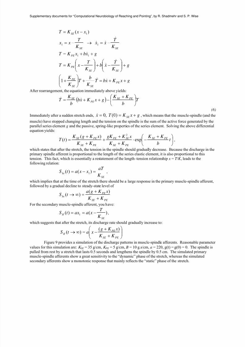
Figure 9 provides a simulation of the discharge patterns in muscle-spindle afferents. Reasonable parameter values for this simulation are: Κ SE = 35 g/cm, Κ PE = 5 g/cm, B = 10 g.s/cm, a = 220, g(t) = g(0) = 0. The spindle is

pulled from rest by a stretch that lasts 0.5 seconds and lengthens the spindle by 0.5 cm. The simulated primarymuscle-spindle afferents show a great sensitivity to the “dynamic” phase of the stretch, whereas the simulated

secondary afferents show a monotonic response that mainly reflects the “static” phase of the stretch.




0.5 1 1.5 2 2.5

1

1.1

1.2

1.3

1.4

1.5

0.5 1 1.5 2 2.5

60

70

80

90

100

110

0.5 1 1.5 2 2.5

180

200

220

240

260

Time (sec)

)(t x

Ia afferent

II afferent

Figure 9. Simulation of the dynamics of a muscle spindle. Muscle undergoes a stretch and this causes

changes in the discharge of the primary- and secondary spindle afferents.

Now consider how the velocity of stretch might affect the activity of the spindle afferents. Assume that you stretch

a spindle 0.5 cm but at a very slow rate, 5 mm/s. In this case, the effect of the viscosity will be small and,

accordingly, the parallel elastic element will lengthen almost as quickly as the series elastic element. In contrast,

when you stretch the spindle rapidly, for example at a rate of 30 mm/s, the viscosity greatly resists stretch of theparallel elastic element and more of the total stretch in the spindle will be taken up by the series elastic element, at

least at first. Therefore, during a rapid stretch, the primary muscle-spindle afferent will fire much more than during

a slow stretch. These properties create the appearance of a velocity signal, as illustrated both in the model and in

recordings from a cat soleus muscle in Figure 10.




0.5 1 1.5 2 2.5 3

60

70

80

90

100

110

0.5 1 1.5 2 2.5 3

180

200

220

240

260

IaS

Time (sec)

0.5 1 1.5 2 2.5 3

1

1.1

1.2

1.3

1.4

1.5 )(t x

II S

A B

Figure 10. Properties of muscle-spindle afferents. A. Recordings from primary (Group Ia) muscle-spindle

afferents of a cat soleus muscle in response to a 6-mm stretch at various speeds of lengthening. B.

Simulations from a model of the spindle undergoing a similar stretch. Primary spindle afferent activity is

larger for greater speeds of lengthening. [From (Goodwin et al., 1972)]

Role of the γ -motor neuron

As the model in Figure 7 suggests, activity of the γ-motor neuron contracts the spindle and affects the lengths of the

series and parallel elastic elements. This contraction, in turn, affects the discharge of the muscle-spindle afferents.

If your muscle spindles did not have γ-motor neurons, their length changes would simply reflect the length changesin the extrafusal muscle. What benefit does the nervous system gain by having a muscle-spindle system in which

length depends not only on the extrafusal muscles—and therefore the angle of joints—but also on the activity of γ-

motor neurons? As you see in this section, activation of γ-motor neurons allows the CNS to bias the sensitivity of the primary spindle afferents and turns them into a sensor that measures movement errors.

Suppose that you decide to flex your elbow. You CNS activates α-motor neurons that act on the biceps,

producing force in the extrafusal muscles and shortening the muscle along trajectory x(t). In this case, the term

trajectory applies to the change in muscle length as a function of time. Of course, trajectory in this sense has an

obvious relationship with trajectory in the more-usual sense of kinematics: e.g., the movement of the hand in space

as a function of time. Now suppose that the CNS programs the γ-motor neurons based on its expectation of how the

biceps should shorten during this movement. Later chapters deal with this notion of expectation in detail, but for thepresent purpose you can think of this conceptually as the desired (d) trajectory of muscle length as a function of

time: xd (t). As you activate your α-motor neurons, you also activate the γ-motor neurons—a coupling termed α– γcoactivation—and you do so such that if the muscle changes length according to your expectation, tension in the

muscle spindle will not change, i.e., 0)( =t T . You can find this level of intrafusal-fiber force by solving for it in

Eq. (6):

( ) 0 ;)0(-)()()0()( >−−= t xt xK t xbgt g d PE d




The above equation tells you that when your biceps is about to shorten, your CNS must activate the γ-motor

neurons by the amount )(t g to maintain tension in the spindle. Figure 11 shows an example: As the simulated

muscle shortens by 0.5 cm, the desired trajectory programs activity in the γ-motor neuron, which produces force g(t )

in the muscle spindle. This increased tension precisely cancels the decrease in tension due to shortening of the

muscle. Therefore, the series elastic element does not change length and, therefore, the primary muscle-spindleafferent does not discharge. However, because of activating the contractile element in the spindle, the parallel

elastic element has shortened, which causes reduced discharge in the secondary muscle-spindle afferents.

0.5 1 1.5 2 2.5

6

8

10

12

14

16

0.5 1 1.5 2 2.5

0.5

0.6

0.7

0.8

0.9

1

Length change in spindle (cm)

g -motor neuron input g(t )

Time (sec)

)(t x

)(t g

0.5 1 1.5 2 2.5

25

50

75

100

125

150

175

Spindle afferent activity (spikes/sec)

Time (sec)

A B

IaS

II S

Figure 11. Simulation of a muscle spindle shortening by 0.5 cm. A. The γ -motor neuron activity is

programmed based on the desired change in muscle length with a time course of activity modulation that

cancel the change in tension in the muscle spindle. B. As the spindle shortens, there is no change in the

primary muscle-spindle afferent discharge (SIa, solid line). Secondary muscle-spindle afferents continue to

respond to shortening of the muscle (SII , dashed line).

Now suppose that as the biceps muscle shortens, an unexpected perturbation prevents it from flexing the

elbow as much or as fast as desired. The γ-motor neurons have activity that corresponds to the desired trajectory,but—because of this external force—the actual trajectory falls short. When you simulate the dynamics of the

system under this condition, you see that the primary muscle-spindle afferents do not remain silent during the

perturbed movement, but strongly increase their activity, instead (Figure 12). In other words, if, during contraction,

the muscle shortens less than expected, primary muscle-spindle activity increases despite the fact that the muscleshortens. By modulating the activity of the γ-motor neurons, the CNS has gained a mechanism by which it candetect error in a movement: more or faster shortening than expected depresses primary muscle-spindle activity;

whereas less or slower shortening results in the activation of these afferents. Activity in primary muscle-spindle

spindle afferents thus signals less muscle shortening than expected. The CNS deals with this information very

directly: the afferents monosynaptically excite α-motor neurons of the same muscle. Therefore, the error signal acts

through the quickest possible CNS route to further activate the extrafusal muscles, produce more force, and further

shorten the muscle. In order for the primary spindle afferents to act as an error detector, the simulations suggest that

the γ-motor neurons must coactivate with α-motor neurons.




0.5 1 1.5 2 2.5

60

80

100

120

140

160

0.5 1 1.5 2 2.5

0.5

0.6

0.7

0.8

0.9

1.0

Actual length change


Time (sec)

Length of spindle (cm)

IaS

II S

Expected length change

0.5 1 1.5 2 2.5

2550

75

100

125

150

175

0.5 1 1.5 2 2.5

0.3

0.4

0.5

0.6

0.7

0.8

0.9

1.0

Expected length change

Actual length change


Time (sec)

Length of spindle (cm)

A B

IaS

II S

Figure 12. Simulation of a muscle spindle that is shortening by an amount that is less than or greater

than the desired trajectory. A. The condition in which perturbations cause the length change to be less

than desired . B Length change is more than desired. Because of the mismatch between the tension

produced by the γ -motor neurons and the tension changes due to shortening of the muscle, primary muscle

spindle afferents (SIa, dashed line) strongly increase their activity (A) or showed depressed discharge rates(B). This is an error signal that indicates the muscle did not shorten as much as it was expected (increased

firing) or shortened more than was expected (decreased firing). Secondary muscle-spindle afferents (SII ,

solid line) do not have this property. Instead, their activity more faithfully reflects muscle length, although

the viscous component of the parallel-elastic element in the muscle-spindle pole leads to transient

deviations from a pure length signal (arrow).

In contrast, activity in the secondary spindle afferents does not reflect an error signal but instead send to the

CNS a fairly faithful measure of actual muscle length—with brief deviations from a pure length signal due to the

viscous component of the parallel elastic element. These neurons lack monosynaptic input on the α-motor neurons,

but instead act on interneurons in the spinal cord, some of which receive inputs from the brain.

Spinal feedback control system

In the section above entitled Simulation of passive properties, you saw how the passive, spring-like properties

of muscles provide a line of defense against perturbations. The model developed in this chapter shows how afferent

feedback from muscles provides a second line of defense. Errors and instability provoked by external perturbations

can be meliorated, if not corrected, by a combination of these active and passive muscle properties: primary muscle-spindle afferents appear to play the largest role during rapid movements, with secondary afferents doing so during

maintenance of steady posture.




Figure 13 schematically summarizes the functions of the muscle-spindle and golgi-tendon-organ afferents

in terms of a feedback control system. Inputs to α-motor neurons cause muscles to produce force that acts on

tendons, shortens muscles, and changes joint angles. Muscle-spindle afferents sense changes in muscle-length, as

biased by activity in the γ-motor neurons. The golgi tendon organs sense force changes, with their signal to

inhibitory interneurons modulated by the descending inputs.The feedback control system rejects perturbations and helps ensure that the limb follows the desired

trajectory. Two locations in the model adjust outputs: one modulates the level of γ-motor-neuron activation, theother does so for the interneurons that golgi tendon organs act on. Consider a situation in which the load exceeds

expectations. For example, you see a milk carton you assume to be empty, so you decide to dispose of it. When you

begin to lift the carton after grasping it, its weight—the load on your muscles—is more than expected. The prime-

mover muscles will shorten, but because of the increased load, they will not shorten as much as expected for an

empty milk carton. You saw earlier that the γ-motor neuron activity is set based on the expected length change in

the muscle. When the muscle shortens less than expected, afferent signals further activate the α-motor neuron,

producing more force, and countering the effect of the load, at least to some extent. The force feedback system,

mediated by the golgi tendon organ, works similarly. As depicted in Figure 13, inputs signaling force from the golgitendon organs inhibit activity in motor neurons via a spinal interneuron. This influence would have the effect of a

negative feedback loop in which high levels of force result in decreasing the motor command and therefore

moderating the force. By inhibiting the interneuron that the golgi tendon organ acts upon (unfilled arrow in Figure

13), descending inputs can modulate how effectively force feedback inhibits the α-motor neurons. Strong inhibition

from the descending inputs imposes a high threshold for the force feedback pathway. Only if the force exceeds thisthreshold will the feedback pathway inhibit the α-motor neuron.

Length (secondary muscle-spindle afferents)

Length error (primary muscle-spindle afferents)

Velocity (primary muscle-spindle afferents)

Gamma bias

Spindles

LoadTendon

organs

Inter-neurons

Length & velocity

feedback

Force feedback

Force controlsignal

Muscle force

Externalforces

Musclelength

Muscleα

γ

Length controlsignal

Drivingsignal

Figure 13. A model of the spinal controller. Schematic of the spindle and golgi tendon

organ feedback system.

Reference List




Bessou P, Emonet-Denand F, and Laporte Y (1965) Motor fibres innervating extrafusal and intrafusal muscle fibres

in the cat. J.Physiol 180: 649-672

Goodwin GM, McCloskey DI, and Matthews PBC (1972) The contribution of muscle afferents to kinaesthesia

shown by vibration induced illusions of movement and by the effects of paralysing joint afferents. Brain

95: 705-748

Hill AV (1970) First and last experiments in muscle mechanics. Cambridge University Press: Cambridge

Inbar GF, and Adam D (1976) Estimation of muscle active state. Biol.Cybern. 23: 61-72

McMahon TA (1984) Muscles, reflexes, and locomotion. Princeton University Press: Princeton, N.J.

a simple muscle model

Documents