a simple method for estimating and testing minimum-evolution …test.scripts.psu.edu/nxm2/1992...

A Simple Method for Estimating and Testing Minimum-Evolution Trees ’

Andrey Rzhetsky and Masatoshi Nei Institute of Molecular Evolutionary Genetics and Department of Biology, Pennsylvania State University

A simple method for estimating and testing phylogenetic trees under the principle of minimum evolution (ME) is presented. The basic procedure of this method is first to obtain the neighbor-joining (NJ) tree by Saitou and Nei’s method and then to search for a tree with the minimum value of the sum (S) of branch lengths by examining all trees that are closely related to the NJ tree. Once the ME tree is identified, a statistical test is conducted for the difference in S between this tree and other closely related trees. The mathematical method required for conducting this test is developed by using the least-squares approach. Computer simulation has shown that this method identifies the correct tree with a high probability, as long as the number of nucleotides examined is sufficiently large. It has also been shown that the topology of the NJ tree is almost always identical with that of the ME tree. A method for obtaining least-squares estimates (and their standard errors) of branch lengths for a given topology is also presented. This method can be used for testing the reliability of the branching pattern of the ME tree. However, the statistical test of S values is more powerful in rejecting incorrect trees than is the branch-length test or bootstrapping. Furthermore, both a mathematical method for computing the number of trees with a given value of topological difference from the NJ tree and a computer algorithm for identifying all the topologies are developed.

Introduction

The neighbor-joining (NJ) method of phylogenetic inference (Saitou and Nei 1987) seems to be quite efficient in obtaining the correct tree, compared with maximum parsimony and several other methods (Saitou and Nei 1987; Sourdis and Nei 1988; Saitou and Imanishi 1989). In this method pairwise distances with multiple-hit cor- rections are used, and a tree is constructed by the principle of minimum evolution (ME), i.e., searching for the tree topology that gives the minimum sum of branch lengths. The ME principle used here is different from that of Cavalli-Sforza and Edwards ( 1967), whose purpose was to construct a Steiner tree. Unlike Saitou and Imanishi’s ME method, however, it does not compute the sum (S) of branch lengths for all possible topologies. Instead, examination of different topologies is imbedded in the algorithm, so that only one final tree is produced. Conducting a computer simulation, Saitou and Imanishi ( 1989) showed that the tree obtained by this method is almost always identical with the ME tree obtained by Saitou and Imanishi’s procedure.

Nevertheless, there is some chance that the NJ tree is different from the ME tree.

1. Key words: neighbor-joining method, minimum-evolution method, estimates of branch lengths, test of topological difference.

Address for correspondence and reprints: Masatoshi Nei, Institute of Molecular Evolutionary Genetics, 328 Mueller Laboratory, The Pennsylvania State University, University Park, Pennsylvania 16802.

Mol. Biol. Evol. 9(5):945-967. 1992. 0 1992 by The University of Chicago. All rights reserved. 0737-4038/92/0905-0014$02.00

945

946 Rzhetsky and Nei

Furthermore, some investigators are interested in comparing the S value for the NJ tree with the S values for other tree topologies. If the NJ tree gives an S value that is significantly smaller than that for any other topology, we can assume that the NJ tree is better than other trees (see Discussion). By contrast, if there is a tree that shows a smaller S value than that for the NJ tree, we should accept it as the most probable tree. Therefore, it is important to know the S values for alternative topologies.

When the number of DNA sequences (n) examined is small (n I 6), it is relatively easy to examine all possible topologies. For a large ~1, however, this method requires a prohibitive amount of computer time. For this reason, Nei ( 199 1) suggested that S be computed only for those trees whose topological distance (dr) from the NJ tree, as measured by Robinson and Foulds’s ( 198 1) method, is equal to 2. Since the number of such trees is small compared with the total number of possible trees, this procedure will greatly facilitate the computation and statistical test of S values for most likely trees. Actually, even if we include the trees with dT = 4, the computation is not necessarily burdensome.

The purpose of this paper is to implement this idea and present the statistical methods required, using a new procedure for obtaining S values for different tree topologies. We also present results of a computer simulation to examine the validity of our statistical methods.

Algorithm

The algorithm we present here is as follows: ( 1) Construct an NJ tree by using Saitou and Nei’s ( 1987) procedure. (2) Obtain all trees whose topological distance from the NJ tree is dT = 2 or 4. (This procedure may be modified as will be mentioned in Discussion.) (3) Estimate S for all these topologies and compute D = S-S,, and the standard error of D for each tree. (S,, is the S value for the NJ tree.) (4) If D is significantly greater than 0 for each tree, adopt the NJ tree as the most probable tree. However, if there are alternative trees whose S values are not significantly different from SNJ, they must be regarded as potentially correct trees. Furthermore, if there is any tree whose S is smaller than SNJ (D < 0)) we must consider it seriously. (5) Estimate branch lengths and their standard errors, to examine the reliability of branch length estimates. In the following we will show how the above algorithm can be im- plemented, starting with procedure (2).

Finding Topologies with dT = 2 or 4

Penny and Hendy ( 1985) proposed a topological distance called “partition distance,” which is equivalent to Robinson and Foulds’s ( 198 1) distance but is simpler to compute. For unrooted bifurcating trees this distance is twice the number of different ways of partitioning sequences between two different trees. (Partitioning of sequences is done only at interior branches.) As an example, consider trees A and B in figure 1. Both trees are for eight sequences and have five interior branches. It is possible to cut the tree at any interior branch and divide the sequences into two groups. Cutting at some interior branches results in the same partition of sequences in trees A and B but not at other branches. For example, a cut at branch a produces two sequence groups- ( 1,2) and (3,4,5,6,7,8)-in both trees. A cut at branch c, however, produces different partitions in trees A and B. That is, the two groups produced by this cut are ( 1,2,3,4) and (5,6,7,8) in tree A but are (1,2,3,5) and (4,6,7,8) in tree B. Similarly, a cut at branch d produces different partitions in the two trees. In the present example, only these two cuts result in different partitions. Therefore, the topological distance between

Minimum-Evolution Trees 947

(A)

CC) (D) (El FIG. 1 .-Hypothetical trees illustrating various computations discussed in text

the two trees is dT = 2 X 2 = 4. If the two trees have the same topology, dT = 0, and if all interior branches produce different partitions, dT = 10 in this example. The general formula for dT for a pair of arbitrary trees for n sequences is given by

4 = 2[min(ql,q2)-Pl+I41-q2l , (1)

where q1 and q2 are the total numbers of partitions (interior branches) for trees 1 and 2, respectively, and p is the number of partitions that are identical for the two trees. ql and q2 may not be the same when multifurcating trees are involved. For bifurcating trees, however, q1 and q2 are always the same, and dT takes only even values. In general, unrooted bifurcating trees for n sequences have IZ - 3 interior branches, so that the maximum possible value of dT for these trees is 2( n-3).

Let us now consider a tree for n sequences and derive a formula for the number of trees whose topological distance from a given tree is dT = 2. We first consider the simplest case of y1= 4 (trees C, D, and E in fig. 1) . In this case, there are three different topologies, and the topological distance of tree D or E from C is dT = 2. Therefore, the number of trees whose topological distance from tree C is dT = 2 is 2. In the following we denote this number by f(dT = 2).

In the case of II sequences f(dT = 2) can be computed by considering each interior branch separately. As an example, consider tree A in figure 1, which has five interior branches. We first note that any interior branch is connected to four groups of sequences. For example, branch a in tree A of figure 1 is connected to sequences 1, 2, 3 and to the group of sequences 4, 5, 6, 7, and 8. If we denote these four groups of sequences by al , a2, a3, and a4, respectively, this tree can be represented by tree C in figure 1. Therefore, branch a of tree A in figure 1 generates two different topologies with distance dT = 2 (trees D and E in fig. 1). In the following we denote trees C, D, and E by [(al,ad(am)l, [(al,ad(am)l, and [(al,a4)(a2,adl, respectively. The same procedure can be used for any interior branch to generate two different topologies with dT = 2. As mentioned above, an unrooted bifurcating tree for n sequences has n - 3 interior branches. Thus, we have the following general formula:


f(dT=2) = 2(n-3) . (2)

The derivation of the formula for the number of trees whose distance from a given tree is dT = 4 is slightly more complicated (Appendix A), but the final result is rather simple. It is given by

f( dT=4) = 2( n2-4n+3n’-6) , (3)

where n’ is the number of tree nodes that are connected to one interior branch and two exterior branches (n24). For example, in tree A in figure 1, n = 8 and n’ = 3, so f (dT=4) = 70. This number is fairly large but is a small proportion of the total number of possible topologies ( 10,395).

To execute procedure (2) in our algorithm, it is necessary not only to know f( dT=2) and f( dT=4) but also to identify all topologies with dT = 2 or 4. An algorithm for identifying these topologies is presented in Appendix B.

Sum of Branch Lengths for a Given Tree Topology

Once all topologies with dT = 2 or 4 are identified, we must compute S for each of the topologies. Saitou and Imanishi ( 1989) used Fitch and Margoliash’s ( 1967) algorithm to estimate this value, but this method is not statistically very efficient. So, in the present paper we shall use the least-squares method. [The NJ method gives least-squares estimates of branch lengths when n15 (Saitou and Nei 1987).]

Let us consider a hypothetical tree for five sequences given in tree A of figure 2 and use the least-squares method to estimate the branch lengths of the tree denoted byb,,bz,..., and b7. We represent an unbiased estimate of the evolutionary distance between sequences i and j by do. We can than write do’s as follows:

d,z = b, + b2 + e12 9

d13 = b, + b3 + b6 + e13 9

d,c, = b, + b4 + b6 + b, + ~4 ,

d,s = b, + b5 + b6 + b7 + ~5 ,

43 = b2 + b3 + bs + e23 ,

d24 = b2 + b4 + b6 + b7 + e24 ,

d25 = b2 + bS + b6 + b7 + e2, ,

d34 = b3 + bq + b7 + e34 ,

4s = b3 + b5 + b7 + e35 ,

45 = h + b5 + e45 ,

where eU’s are sampling errors. We assume that ei, is distributed with mean 0 and


variance I’( d,). If we use matrix algebra, the above set of equations may be written as

d=Ab+e, (4)

where d, b, and e are the column vectors of dij’s, hi’s, and c;j’s, respectively, i.e., d’

= (42, 43, *. . 7 &), 6’ = (b,, b2, . . . , b,), and e’ = (ei2, ~3, . . . , ed5). Here t indicates the transpose of vectors or matrices. A is given by

A=

-1100000 1010010 1001011 1000111 0110010 0101011 0100111 0011001 0010101

-0 0 0 1 1 0 0

(5)

The least-squares estimate of b is then given by

6 = (A*A)-‘A’d = Ld, (6)

where L = (AlA)-‘A’. Obviously, an estimate of the length of the ith branch is

bi = Lid, (7)

where Li is the ith row of the matrix L. The variance of 6, is then given by

V( bi) = Li VL$ t (8)

where Y is the variance and covariance matrix of distances, which will be discussed in detail later. Once the branch lengths are estimated, we can easily compute the S of all branch lengths by

SC 2 bi, (9) i=l

where bi is the estimate of branch length bi, and T is the total number of branches. The above approach can be extended to the case of any number of sequences.

When there are y1 sequences, Tin an unrooted bifurcating tree is 2n - 3, and the total number of pairwise distances (R) is n( n - 1 )/ 2. In the following, dii will be renumbered from dl to dR, depending on the convenience.

For obtaining S, however, it is not necessary to estimate all branch lengths. Since S is a linear function of du’s, it can be obtained without estimating bi’s. That is,


S=yd, (10)

where y is a row vector of the coefficients of di’S, i.e., y = (vi, ~2, . y can be obtained by

y = A(A’A)-‘U,

) yR). The vector

(11)

where u is a unit column vector of 2n - 3 elements, i.e., U’ = ( 1, 1, the least-squares estimate of S is

S = yd = A(A’A)-‘ud = 2 yidi . i=l

. 3 1) . Therefore,

(12)

In the case of tree A in figure 2, y becomes

yA = (l/z, ‘/4, i/8, l/s, i/i, i/s, Ys, l/4, vi, ‘/2) .

So, S is given by

(13)

S, = L/2 + &/4 + 448 + 448 + 43/J

+ dxl8 + d&J + d&4 + i&s/4 + &I2

Similarly, for tree B in figure 2, we have

y a = ( ‘4 l/2, ‘h, l/s, G, vi, l/4, %, ‘18, ‘/2) )

S, = d&4 + &I2 + d,4/8 + du/8 + dz3l4

+ d&4 + dxl4 + &I8 + d&8 + de/2

Test of the Null Hypothesis D = S&~‘A = 0

(14)

(15)

(16)

As mentioned earlier, we are primarily interested in the difference in S between two topologies. This difference can be written as

D = SB-SA = (yB-y,)d = i (yBi-yAi)d;. i=l

(17)

Therefore, if yA and yB are computed for a pair of topologies, D can easily be obtained.

(A) (Bl (Cl FIG. 2.-Hypothetical trees illustrating computation of branch lengths and S values

Minimum-Evolution Trees 95 I

For this purpose, it is not necessary to know individual S values. In the case of trees A and B in figure 2, we know Yni’s and ysi’s, so D is given by

D = -d&4 + d&4 + d&3 + dz& - djd/S - d&I . (18)

Our null hypothesis is D = 0, as mentioned earlier. If S, is smaller than SB and D is significantly greater than 0, we conclude that tree A is better than tree B. However, what is the biological meaning of this null hypothesis when two different topologies are compared? Actually, this hypothesis is equivalent to the null hypothesis that the lengths of the interior branches that produce different partitions of sequences for the two topologies are 0. For example, the test of D = SB-S, = 0 in the trees of figure 2 is actually testing the hypothesis that b6 = 0. Indeed, we can show that

D = &--S, = b6/2-(2e12-2e13-e24-e25+e34+e35)/8 . (19)

Therefore, when b6 = 0, the expectation of D is 0. In practice, we do not know which of trees A and B is the correct one. So, D can be positive or negative. Similarly, D = SC-S, can be written as

D = SC-S,, = 3(b6+b7)/4-3(elz-e14-e25+e45)/8 . (20)

Therefore, we are testing the null hypothesis that both b6 and b7 in tree A in fig. 2 are equal to 0. This principle applies to any pair of bifurcating trees, irrespective of the number of sequences.

Variance of D = S,-SB

To test the statistical significance of D, however, we must compute the variance of D. Nei ( 199 1) suggested that the variance of D be computed by the bootstrap method (Efron 1982, chap. 5). However, the variance of D, V(D), can be obtained analytically. That is,

v(D) = bwyd’~/(yrYA) (21)

= g (Y~i-YAi)2Vdi)+2 5 (Y~i-YAi)(Y~j-Y~j)COV(di,dj) . i=l js-i

Here, V stands for the variance-covariance matrix of dil’s. In the case of trees A and B in figure 2, V(D) can be written as

v(D) = v( &)I 16 + V( dnU16 + V( &)I64 + J’( &)I64

+ v( &)I64 + V(&)l64 - Cov(dmddl8 - Cov(dn,dz,)ll6

- Cov(&,&)l16 + Cov(dn,&)l16 + Cov(&,&)ll6

+ Cov(dn,&)l16 + Cov(d,3,dz)l16 - Cov(dddll6 (22)

- Cov(&,&)l16 + Cov(&,&)l32 - Cov(dddl32

- Cov(&,d35)/32 - Cov(dzs,ddl32

- Cov(&,&)l32 + Cov(&,45)/32.


There is no difficulty in evaluating I’( dij). Most methods for estimating dij from sequence data give an approximate formula for V( dV) (e.g., see Kimura and Ohta 1972; Kimura 1980; Tajima and Nei 1984). However, the computation of Cov( do, dlk) is more complicated.

A number of authors (e.g., Nei et al. 1985; Bulmer 1989; Nei and Jin 1989) have proposed use of the formula

where db,kl is the length of branches that are shared by the path connecting sequences i and j and the path connecting sequences k and 1. Hence, the estimation of Cov( dii, dkl) depends on tree topology. Since two different tree topologies are involved in our case, this approach is inapplicable. We therefore use the method suggested by Bulmer (1991).

Let dij be the distance between species i and j, and let dkl be the distance between species k and 1. The correlation coefficient between dij and dkl may be estimated by

(Pij,kl-PijPkl)

rv*k’ = [ ( 1-&)&( 1 -pk,)pk[] “2 ’ (24)

where pij,k/ is the proportion of sites at which sequence i differs from sequence j and sequence k differs from sequence 1, and where pij is the proportion of sites at which sequence i differs from sequence j. Therefore, COV(diirdk,) can be estimated by

where s( d,) and s( dkl) are the standard deviations of dii and dki, respectively. In the case of Jukes and Cantor’s ( 1969) one-parameter model the evolutionary distance between a pair of sequences is estimated by

do = -b ln( 1-p,/b) , (26)

where b = 31’4, and the variance of dil is given by

V( do) = Pijt l -Pij)

m( 1-PJb)2 (27)

(Kimura and Ohta 1972). Here, m stands for the number of nucleotides examined. The covariance of du and dkj is therefore given by

cov( dti,dk,) = (PijKPijPRI)

m( l-PJb)( I-PkJb) (28)

(Bulmer 199 1). The formula can also be used for amino acid sequence data by putting b = 19/20. In the case of Kimura’s ( 1980) two-parameter model, we have


do = --l/z ln[( l-2P,-QU)dl-2QU], (29)

Var( d,) = ( 1 /m)[( a$Po+b$Q,)-( a~P~+bijQ~)*] , (30)

Cov( dij,dk,) = (&j,kl-PijPkl)

m[( l-PV)Pij( l-Pkl)Pklll’*

X [ (a~P~+b~Q~)-( a~P~+b~Q;j)*] “*

x [(a:rPkl+btrQk,)-(akIPkr+bklQk/)*l “* ,

(31)

where P, is the proportion of transitional differences between species i and j, Qii is the proportion of transversional differences between species i and j, aij = (l-2P,-Q,)-‘, and be = (l/2)( 1-2P~-Q~)-‘+(Y2)( 1_2Qij)-l. (See note added in proof.)

Computer Simulation

The method of obtaining the ME tree presented in this paper depends on a number of assumptions. In particular, it assumes that the ME tree is included in the group of trees whose topological distance dT from the NJ tree is 2 or 4 and that the ME tree is likely to be the correct tree. (Of course, when the number of sequences is small, it is possible to examine all possible trees.) Furthermore, the resolving power of our test of D = S-S,.,, is dependent not only on the lengths of the interior branches involved but also on the error terms eU’s [ eqq. ( 19) and (20)]. We therefore examined the validity of the assumption and the resolving power of our phylogenetic test by using computer simulation.

Probability of Obtaining the True Tree among the Neighboring Trees of the NJ Tree

Our first simulation was conducted to see how close the NJ tree is, compared with the true tree. We set up a model tree and simulated nucleotide substitution according to this model tree. The method of the simulation of nucleotide substitution was the same as that of Sourdis and Nei ( 1988), but we considered only the Jukes- Cantor model of substitution. The model trees considered were the same as those of Saitou and Imanishi ( 1989) and consisted of six DNA sequences (fig. 3) with various topologies and branch length. (We also considered several other trees with 10 sequences, but, since the results obtained were essentially the same as those for fig. 3, we shall not present them.) Nucleotide substitution was assumed to be stochastic, so that the sequences generated for a given model tree varied from replication to replication. Once a set of six extant sequences were generated for a given tree, a tree was reconstructed by the NJ method, and this tree’s topological distance from the true tree was computed. This was repeated 10,000 times for each tree. In trees A and B in figure 3 a constant rate of evolution was assumed for all sequences, whereas in trees C and D in figure 3 the rate of nucleotide substitution varied with sequence. In these trees the branch lengths are proportional to the expected number of substitutions per site. In the case of constant rate of substitution (i.e., trees A and B), the expected number of substitutions per site, from the ancestral sequence to the extant sequence, is denoted by I-J, and the length of each branch is expressed as multiples of a, which is related to U as specified in each figure. We examined two different values of U, namely, 0.05


4a

(A) 4a 1

a 2 (B)

CD)

6a a , 1 6a 7a

2

7” 3 ,a

6a 4

6a 5 6

FIG. 3.-Four model trees used for computer simulation. These trees are identical with those used by Saitou and Imanishi ( 1989).

and 0.5. In the case of varying rate of evolution (i.e., trees C and D), a = 0.01 and a = 0.05 were used. These values are identical with those used by Saitou and Imanishi ( 1989 ). In each of the four trees, we considered five different numbers of nucleotides examined, m, i.e., 300, 600, 900, 1,200, and 2,400.

Table 1 shows the relative frequencies of the NJ trees differing from the true tree by dT = 0, 2, 4, and 6, for model trees A and B. Here dT = 0 denotes the case where the NJ method recovered the correct tree. The frequencies in table 1 are similar to

Table 1 Frequencies of NJ Trees Differing from Correct Tree by dT = 0, 2,4, and 6

FREQUENCYOF

(S)

Tree A: dT = Tree B: dT =

0 2 4 6 0 2 4 6

u = 0.05: 300 bp 600 bp 900 bp 1,200 bp _. _. 2,400 bp

u = 0.50:

58.1 31.7 8.7 1.5 62.9 31.7 5.1 0.3 82.1 16.3 1.5 0.1 84.3 14.8 0.9 0 92.6 7.0 0.4 0 92.9 6.9 0.2 0 96.2 3.8 0.1 0 96.6 3.3 0.1 0 99.7 0.3 0 0 99.8 0.2 0 0

300 bp 53.6 34.7 10.3 1.3 52.8 39.2 7.9 0.1 600 bp 79.8 18.6 1.6 0.1 76.7 21.9 1.4 0 900 bp 93.0 7.0 0 0 91.0 8.8 0.2 0 1,200bp .._. 96.3 3.7 0 0 96.4 3.6 0 0 2,400 bp 99.6 0.4 0 0 99.7 0.3 0 0

NOTE.-& = 0 represents the correct topology. These results are based on 10,000 replications.


those obtained by Saitou and Imanishi ( 1989), though these authors examined only the cases of m = 300 and m = 600. When m = 300; the NJ method may choose a wrong tree, with a substantial probability. However, if we consider the trees with dr I 4, the correct tree is included among them with a probability of 98.5%. This probability increases to nearly 100% if m 2 600. Actually, in the case of m 2 600, the probability of finding the correct tree among trees with dT I 2 from the NJ tree is >0.98. The results are essentially the same both for trees A and B and for U = 0.05 and 0.50. The same thing can be said about trees C and D in figure 3 (table 2). Furthermore, we examined four more trees with 10 DNA sequences, as mentioned earlier. In these cases, too, the probability that the correct tree is included among the trees with dT 5 2 was very high, as long as m is large (2900). Therefore, our procedure seems to be sufficient for obtaining the correct tree when topologies with dT I 2 are considered, as long as m > 900. (Of course, if a is very small, this would not be the case, and some other procedures are necessary, as will be mentioned in Discussion.)

Rank of S for the True Tree among the Neighboring Trees with dT = 2

Theoretically, the true tree is expected to give the smallest S value, compared with other trees, as long as dij’s are unbiased estimates and m is large (authors’ unpublished data). In practice, however, sampling errors may disturb the ranks of S values. We therefore examined the rank of the S for the true tree among the trees with dT I 2. Table 3 shows that in both tree A and tree B the probability that the S for the true tree is smallest is -5O%-60% when 300 nucleotides are examined but that the probability rapidly increases as m increases. Yet, it is ~98% even for m = 1,200. It is interesting to see that these values are virtually identical with the probabilities that the NJ tree is the correct tree in table 1. They are also similar to the probabilities that the ME tree is the correct tree (Saitou and Imanishi 1989). These results support Saitou and Imanishi’s ( 1989) conclusion that the NJ tree is almost always identical

Table 2 Frequencies of NJ Trees Differing from Correct Tree by dT = 0, 2,4, and 6

FREQUENCYOF (%I

Tree C: dT = Tree D: dT = .._

0 2 4 6 0 2 4 6

_ a = 0.01:

300 bp 14.6 21.7 3.3 0.4 75.6 19.6 4.6 0.2 600 bp -’ 93.7 6.2 0.1 0 94.5 5.0 0.5 0 900 bp 98.1 1.9 0 0 98.7 1.3 0 0 1,200bp _.... 99.4 0.6 0 0 99.6 0.4 0 0 2,400 bp 100.0 0 0 0 100.0 0 0 0

a = 0.05: 300 bp 72.3 24.0 3.3 0.4 75.8 17.5 6.5 0.1 600 bp : : 90.6 8.6 0.8 0 94.5 4.5 1.0 0 900 bp 91.3 2.7 0 0 99.0 0.9 0.1 0 1,200bp 98.5 1.5 0 0 99.7 0.3 0 0 2,400 bv 100.0 0 0 0 100.0 0 0 0

NOTE.-dT = 0 represents the correct topology. These results are based on 10,000 replications.


Table 3 Frequencies of Rankings of S Value for True Tree among Trees with & I 2

FREQUENCY OF (%I

Tree A: Rank of S = Tree B: Rank of S =

1 2 3 4 5 1 2 3 4 5

u = 0.05: 300 bp _. 600 bp 900 bp 1,200bp 2,400 bp

u = 0.5:

57 23 16 3 0 63 21 14 2 0 83 12 5 0 0 84 12 4 0 0 94 5 1 0 0 94 6 1 0 0 97 3 0 0 0 95 4 1 0 0

100 0 0 0 0 100 0 0 0 0

300 bp 51 31 16 2 0 54 31 13 3 0 600 bp 17 18 5 0 0 77 17 5 1 0 900 bp _. 90 9 1 0 0 92 6 1 0 0 1,200bp 96 4 0 0 0 97 3 0 0 0 2,400 bp 99 1 0 0 0 99 1 0 0 0

NOTE.- I, 2,3, . represent the smallest, second smallest, third smallest, etc. These results are based on 1,000 replications.

with the ME tree. Table 4 gives the same quantities for trees C and D. In this case the probability that the true tree shows the smallest S is even higher than that for trees A and B. From these results, we may conclude that, if all trees whose distance from the NJ tree is dT = 2 are examined, the true tree is included with a high probability, unless m and a are very small.

Resolving Power of the Statistical Test Proposed

To examine the resolving power of our phylogenetic test, we studied the frequencies of occurrence of the following four cases: ( 1) the S for the true tree (ST) is minimum and is significantly (5% level) smaller than any other S. (2) Sr is smallest but is not statistically significant from the second smallest S. (3) A wrong tree shows the smallest S value, but it is not statistically significant from Sr . (4) A wrong tree shows the smallest S, which is significantly smaller than Sr.

Table 5 shows the frequencies of these four different cases for trees A and B. When m = 300, the frequency of case ( 1) is quite low, indicating the inefficiency of our statistical test. Furthermore, for m = 300, case (4) occurs with a frequency of 0.5%- 1%. Even when m is as large as 2,400, the frequency of case ( 1) is not very high. Table 6 shows that the results for trees C and D are better than those for trees A and B. With these model trees the frequency of case ( 1) is - 290% when 2,400 nucleotides are examined. Our test is more powerful in the case where substitution rate varies with evolutionary lineage than in the case where the molecular clock applies. In tables 1 and 2 we saw that the ME tree or the NJ tree is correct with a probability of >99% in the case of m = 2,400. Yet, the S for the correct tree is not always significantly smaller than the second smallest S. In this sense, our test is quite conservative.

Numerical Example

At the present time, the crocodilian group of reptiles is believed to be the type of organism that is most closely related to birds. However, molecular data often suggest


Table 4 Frequencies of Rankings of S Value for True Tree among Trees with dT I 2

FREQUENCY OF (%I

Tree C: Rank of S = Tree D: Rank of S =

1 2 3 4 5 1 2 3 4 5

a = 0.01: 300bp 600 bp 900 bp 1,200 bp 2,400 bp

a = 0.05: 300 bp 600 bp 900 bp 1,200 bp 2,400 bp

73 19 7 1 0 76 17 7 0 0 92 7 1 0 0 97 3 0 0 0 98 2 0 0 0 99 1 0 0 0 99 1 0 0 0 100 0 0 0 0

100 0 0 0 0 100 0 0 0 0

70 24 6 0 0 a2 14 4 0 0 90 9 1 0 0 97 3 0 0 0 97 3 0 0 0 100 0 0 0 0 99 1 0 0 0 100 0 0 0 0

100 0 0 0 0 100 0 0 0 0

NOTE.-I, 2,3, represent the smallest, second smallest, third smallest, etc. These results are based on 1,CKM replications.

that birds are more closely related to mammals than to reptiles. Hedges et al. ( 1990) recently studied this problem by using the nucleotide sequences of the 18s ribosomal RNA gene and some other data. We therefore examined this problem by using our new statistical method.

Table 5 Results of Significance Tests of D = S-ST

FREQUENCY OF

(%)

Tree A: Case Tree B: Case

1 2 3 4 1 2 3 4

u = 0.05: 300bp 600bp 900bp 1,200 bp 2,400 bp

u = 0.5: 300 bp 600 bp 900bp 1,200 bp 2,400 bp

0 56.9 42.7 0.4 0 64.8 34.7 0.5 0.4 81.8 17.6 0.2 1.6 83.2 15.0 0.2 3.7 89.2 6.9 0.2 8.7 83.0 8.2 0.1

12.3 83.7 4.0 0 20.8 75.2 4.0 0 71.3 28.7 0 0 71.2 28.6 0.2 0

0 52.2 47.3 0.5 0 50.3 48.8 0.9 0.6 76.9 22.4 0.1 0.9 77.7 21.2 0.2 5.6 85.3 9.1 0 7.2 84.4 8.3 0.1

17.1 79.9 3.0 0 20.7 74.9 4.4 0 58.4 41.1 0.5 0 57.9 41.2 0.9 0

NOTE.--I = Significant minimum ofthe S for the true tree (S,); 2 = nonsignificant minimum of&; 3 = nonsignificant minimum of S for a wrong tree; and 4 = significant minimum of S for a wrong tree. These results are based on 2,000 replications.


Table 6 Results of Significance Tests of D = S-ST

FREQUENCYOF

@b)

Tree C: Case Tree D: Case

1 2 3 4 1 2 3 4

a = 0.01: 300bp 600bp 900 bp 1,200 bp 2,400 bp

a = 0.05: 300bp 600bp 900bp 1,200 bp 2,400 bp

0.1 13.4 26.2 0.3 0.1 78.1 21.5 0.3 4.9 88.5 6.6 0 7.8 87.6 4.6 0

23.6 73.8 2.5 0.1 31.0 67.1 1.3 0 44.4 54.3 1.3 0 51.1 42.2 0.1 0 95.2 4.1 0.1 0 98.6 1.4 0 0

0 10.7 29.2 0.1 0.2 80.7 19.1 0 2.0 87.0 11.0 0 9.6 86.6 3.8 0

16.1 19.6 4.3 0 42.2 57.0 0.8 0 40.4 58.2 1.4 0 71.4 28.5 0.1 0 89.4 10.5 0.1 0 99.3 0.7 0 0

NOTE.-1 = Significant minimum ofthe S for the true tree (&); 2 = nonsignificant minimum of&; 3 = nonsignificant minimum of S for a wrong tree; and 4 = significant minimum of S for a wrong tree. These results are based on 2,COO replications.

In this numerical example we will use the nucleotide sequences of the 18s ribosomal RNA gene for six species: Homo sapiens (mammal), Turdus migratorius (bird), Heterodon platyrhinos (snake), Xenopus laevis (frog), Pseudemus scripta (turtle), and Alligator mississippiensis (crocodilian). Hedges et al. have presented the entire sequences available for these species. In this analysis, however, we eliminated all deletions/insertions (gaps) and ambiguous nucleotide sites and used 1,297 sites which were shared by all the six species. We first estimated the number of nucleotide substitutions per site (d) for all pairs of sequences by using the Jukes-Cantor formula. [In the present case, most distance measures give essentially the same results, since the d is small (Nei 1987, pp. 72-73).] The results ‘obtained are presented in table 7. Using the NJ method, we then reconstructed a phylogenetic tree, which is presented as tree A in figure 4. The branch lengths of this tree and their standard errors were estimated by the least-squares method described earlier [ eqq. (6) and ( 8)], The sum of all branch lengths therefore becomes 8.27 X lo-‘. For this case, the matrix L in equation (6) is given in figure 5.

Table 7 Pairwise Distances (d X 100) for Six Species of Tetrapods

Bird Snake Frog Turtle Crocodilian

Mammal Bird Snake Frog Turtle Crocodilian

3.31 3.31 4.61 3.06 2.82 3.39 5.35 3.31 2.98

3.63 1.63 1.16 3.06 2.14

0.46


Snake Frog Turtle

Mammal S = 8.27 Crocodile

d,= 2

(6) ;>g<; S-8.63 (C) :$<I s=8.71

(D) I>%<: S-837 (E) :>r4: s-830

F S

Y-k T s=t330

C

d,= 4

F r

0-I) ;>-&<; s=a44 (I)

S S = 8.40

c

(J) I>+--<; s-8.40 (K) I$<; s=844

FIG. 4.-NJ tree (A) and its closely related trees (B-K) for the 18s rRNA genes from six tetrapod species [mammals (M), birds (B), snakes (S), frogs (F), turtles (T), and crocodiles (C)l. The estimates of branch lengths (i.e., b X 100) and their standard errors were obtained by the least-squares method. The estimate of the length of a branch with a (-) sign was negative. The S value in this figure represents the true value multiplied by 100.

With six species, there are 105 different topologies. Six of them have a topological distance of dT = 2 from the NJ tree. These six topologies are given as trees B-G in figure 4. To compute S and D = S-S,, for all of these topologies, we must know the vector (y) of y coefficients [ eq. ( lo)]. These vectors for topologies A-G can be obtained by using equation ( 11). For example, the vectors for trees A and G are as follows:


111111111 ---- i i i 8 --- a a -- 8 8 8 0 0 0

111111111 - -- -- -- -- i i i i 0 0 0 2 8 a 8 0

11111111111 0 ------- - - --- 4 12 12 12 t i? 12 12 a a 6

1 1 1 0 0 _-2-G 0 -__&g ___$; 6 6 6

1 1 1 L- 0 0 0 --i 0 0 --+ 0 --!j a 8 8

1 1 1 0 0 0 -i 0 0 -; 0 -; i i i

111111111111 -- 4 12 12 12 G 12 1212 - -- -- -_ 2 6 6 6

5 1115 112 5 5 0 -; - -- 36 Is 18 4 36 ls ls 9 36 36

11 11111 0 0 -f 0 -; - -- 12 12 T? 12 6 12 is

FIG. 5.-Matrix L in eq. (6), for tree (A) in fig. 4

0

0

0

1 i;

1 i

1 -- 8

0

1 -- 4

1 4

0 0

0 0

0 0

1 T

0

11 -- 8 i

11 i i

0 0

1 -- 0 4

11 - -- 4 2

y/+=(1/21/45/31/ ‘/ ‘/ ‘/ ‘/ 5 ‘/ 7 ‘/ ‘/ 7); 6 18 18 4 18 18 9 36 36 4 4 2

YG’(l/ 288888888288882. ‘/ 7 ‘/ ‘/ 7 7 7 7 ‘/ ‘/ ‘/ 7 7 ‘/I

The vectors ya, yc, yo, yr, and yr can be readily obtained from yA by renumbering of yi’s. The S values obtained from these vectors [see eq. ( lo)] are given for each of the topologies in figure 4. These values indicate that the NJ tree (tree A) has the smallest S but that several other trees have an S that is close to the smallest S, i.e., SNJ.

To test the statistical significance of the difference (D) in S between tree A and another tree, we must compute the variance of D given by equation ( 2 1) , The variances and covariances in matrix Yin this equation can be obtained by using equations (27) and (28). One can therefore compute the standard error of Di = simsA by

S(Di) = [(Yi-YA)'V(Yi-yA)]1'2 3 (32)

where the subscript i refers to the ith tree. This computation gives the following results { [Di+S(Di)]XlOO}: 0.36 + 0.16 for tree B, 0.44 + 0.15 for tree C, 0.10 +- 0.07 for tree D, 0.11 +- 0.06 for tree E, 0.12 +- 0.08 for tree F, and 0.03 f 0.08 for tree G. Therefore, a 2 test [Z = D/s(D)] shows that the NJ tree is significantly better than trees B and C (at the 5% level), whereas the S values for other trees (D-G) are not significantly different from S,, . Therefore, we have to consider any of the latter four trees and the NJ tree as a potentially correct tree.

In addition to these trees presented in figure 4 (i.e., trees A-G), there are 98 more different topologies in the present case. We computed the S values for all of these topologies and found that the S value for four more topologies are not signifi-

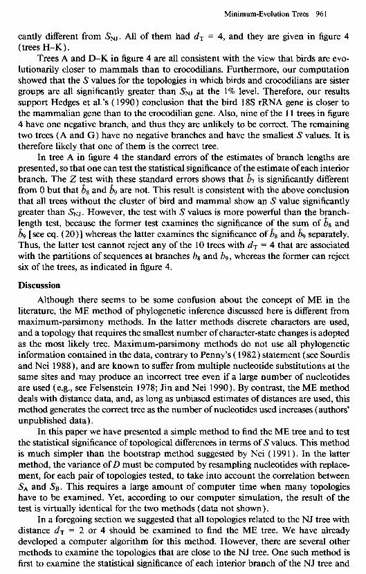
Minimum-Evolution Trees 96 I

cantly different from SNJ. All of them had dT = 4, and they are given in figure 4 (trees H-K).

Trees A and D-K in figure 4 are all consistent with the view that birds are evo- lutionarily closer to mammals than to crocodilians. Furthermore, our computation showed that the S values for the topologies in which birds and crocodilians are sister groups are all significantly greater than S NJ at the 1% level. Therefore, our results support Hedges et al.3 ( 1990) conclusion that the bird 18s rRNA gene is closer to the mammalian gene than to the crocodilian gene. Also, nine of the 11 trees in figure 4 have one negative branch, and thus they are unlikely to be correct. The remaining two trees (A and G) have no negative branches and have the smallest S values. It is therefore likely that one of them is the correct tree.

In tree A in figure 4 the standard errors of the estimates of branch lengths are presented, so that one can test the statistical significance of the estimate of each interior branch. The Z test with these standard errors shows that b, is significantly different from 0 but that 6, and 6, are not. This result is consistent with the above conclusion that all trees without the cluster of bird and mammal show an S value significantly greater than SNJ . However, the test with S values is more powerful than the branch- length test, because the former test examines the significance of the sum of 6, and 6, [see eq. (20)] whereas the latter examines the significance of & and 6, separately. Thus, the latter test cannot reject any of the 10 trees with dT = 4 that are associated with the partitions of sequences at branches bs and b9, whereas the former can reject six of the trees, as indicated in figure 4.

Discussion

Although there seems to be some confusion about the concept of ME in the literature, the ME method of phylogenetic inference discussed here is different from maximum-parsimony methods. In the latter methods discrete characters are used, and a topology that requires the smallest number of character-state changes is adopted as the most likely tree. Maximum-parsimony methods do not use all phylogenetic information contained in the data, contrary to Penny’s ( 1982) statement (see Sourdis and Nei 1988), and are known to suffer from multiple nucleotide substitutions at the same sites and may produce an incorrect tree even if a large number of nucleotides are used (e.g., see Felsenstein 1978; Jin and Nei 1990). By contrast, the ME method deals with distance data, and, as long as unbiased estimates of distances are used, this method generates the correct tree as the number of nucleotides used increases (authors’ unpublished data).

In this paper we have presented a simple method to find the ME tree and to test the statistical significance of topological differences in terms of S values. This method is much simpler than the bootstrap method suggested by Nei ( 199 1). In the latter method, the variance of D must be computed by resampling nucleotides with replace- ment, for each pair of topologies tested, to take into account the correlation between S, and SB. This requires a large amount of computer time when many topologies have to be examined. Yet, according to our computer simulation, the result of the test is virtually identical for the two methods (data not shown).

In a foregoing section we suggested that all topologies related to the NJ tree with distance dT = 2 or 4 should be examined to find the ME tree. We have already developed a computer algorithm for this method. However, there are several other methods to examine the topologies that are close to the NJ tree. One such method is first to examine the statistical significance of each interior branch of the NJ tree and


then to compute S for all topologies associated with branches whose lengths are not significantly different from 0. In this procedure we can avoid the computation of S for trees that have dT = 2 or 4 but that will probably have a significantly larger S value as in the case of trees B and C in figure 4. We are currently developing a computer algorithm for this method. When there are many small interior branches and the number of nucleotides examined is not large, this method may identify many nonsignificant interior branches, and consequently one may have to examine a large number of topologies, including those with dT 2 6. In this case, however, it would not be very meaningful to compute the D values for all of these topologies, because there are too many possible trees to permit any meaningful conclusion. In such a case the best way to resolve the topological problem would be to increase the number of nucleotides examined. At any rate, the test of interior branch lengths provides important information for phylogenetic inference.

The statistical method presented in this paper depends on the least-squares estimation of branch lengths. One might therefore wonder whether the ME method is superior to the least-squares phylogenetic-inference method proposed by Cavalli-Sforza and Edwards ( 1967) and Fitch and Margoliash ( 1967). Our theoretical study has indicated that, in obtaining the correct tree, the ME method is statistically more efficient than the least-squares method. Therefore, the ME method is superior to the least- squares method. This result will be published elsewhere.

One of the commonly used methods for testing the reliability of the branching pattern of a tree is the bootstrap test (Efron 1982, chap. 5; Felsenstein 1985; Whittam 1990). This method is equivalent to our test of interior branch lengths (see also Li 1989), and our computer simulation has shown that it gives essentially the same statistical conclusion. In practice, however, it is much easier to use the branch-length test, since this test can be carried out by using analytical formulas. Nevertheless, it should be noted that, in rejecting incorrect trees, the bootstrap and branch-length tests are less powerful than the S-value test, as mentioned earlier.

Computer Program

A computer program for computing all the quantities presented in this paper is available on request.

Acknowledgments

We thank Michael Bulmer, Tatsya Ota, Blair Hedges, and Koichiro Tamura for their comments on an earlier version of this paper. This study was supported by research grants from the National Institute of Health and the National Science Foun- dation to M.N.

APPENDIX A

Number of Topologies with dT 2 4 To obtain the number of trees with dT = 4, we must consider two interior branches

simultaneously. Because there are n - 3 interior branches for an unrooted bifurcating tree with n sequences, it is necessary to consider [(n-3)(n-4)]/2 pairs of interior branches. Some of these pairs of branches are connected with each other, but others are separated by some other branches. In the following, these two different cases will be considered separately.

1. Case of Two Contiguous, Interior Branches When two interior branches are connected with @-other, the sequences involved

can be divided into five groups, al, a2, a3, a4, and a5 (see fig. A 1) . Any of these groups


may include one or more sequences. To generate a topology with dT = 4, a cut of both branches a and b in the new topology must produce different partitions of sequences, compared with those of the original topology (i.e., tree A). A cut of branch a of tree A produces a partition of sequences which may be represented by [(al ,a2)( a3,a4,a5)], and a cut of branch b produces a partition represented by [(al,a2,a3)(a4,a5)]. Therefore, tree A may be described by [(al,a2)(a3)(a4,a5)]. All topologies with dT = 4 can then be generated by rearranging the five sequence groups as follows:

[(al,a3)(a4)(a2,&)1 , [(&,a3)(&>(a2,a4>],

[(al,a4)(a2)(a3,&)1 , [(al>a4)(a3)(a2,a5)1 ,

[(@,a4)(a5)(a2,a3)1, [(@@5)(a3)(a2,a4)1 ,

[(al,a5)(a4)(a2@3)1 3 [(al,a5)(a2)(a3,a4)1 7

[(a2,a4)(al)(a3,a5)1 > t(a2,a5)(al)(a3,a4)1 *

(Al)

These 10 topologies are shown as trees B-K in figure A 1.

2. Case of Two Noncontiguous Interior Branches In this case, each of two noncontiguous branches, say a and c in tree A in figure

1, produces four different groups of sequences and generates two topologies with dT = 2. Therefore, if we consider branches a and c simultaneously, they generate four topologies with dT = 4. In this case, we write the original tree as

al a3

a4 4

I 2

(A) (8) a2 a5

3 5

5 2 3 1 2 1 3 I 2

(C) (D) (E) 3 4 4 5 4 5

5 3 4 I 2 1 2 I 2

(F) (G) (HI 4 3 5 4 5 3

2 1 1 1 3 2 3 2 3

(I) (J) (K1 5 4 4 5 5 4

F~~.Al.-(A),Fivegroupsofsequences(o,,a~,a~,a~,anda~) associated with two contiguous interior branches. The rearrangement of the five groups of sequences generates 10 different topologies [(B)-(K)] with dT = 4.


[(al,~2)(a~,~~)(b~,~2)(~~,b4)1,whereal,a2,~3,~4,~~,~~,~3,and~4repre~nfsequence groups {l}, { 2}, {3}, {4,5,6,7,8}, {1,2,3}, (41, {5,6}, and {7,8}, respectively, in tree A in figure 1. The four topologies may then be written as follows:

(A21

3. Number of Topologies with dT = 4 In a tree with y1 sequences there are IZ + n’ - 6 contiguous pairs of interior

branches, and each of these pairs generates 10 topologies with dT = 4. On the other hand, the number of noncontiguous pairs of interior branches is given by [(n-3)(n-4)]/2 - (n+n’-6), and each ofthese pairs generates four topologies with dT = 4. Therefore, the total number of topologies with dT = 4 is given by

j-( dT=4) = lO(n+n’-6)+4{ [(n-3)(n-4)]/2-(n+n’-6))

= 2( n2-4n+3n’-6) , (A3)

which is identical with equation (3).

4. Number of Topologies with dT 2 6 To compute the number of topologies with dT = 2i, where i is an integer 23, we

must consider all possible combinations of i interior branches, whether they are contiguous or not. In the case of i = 3, for example, there are four different types of combinations of interior branches: (i) three noncontiguous branches, (ii) two contiguous branches plus one noncontiguous branch, (iii) three linear contiguous branches (e.g., branches a-c in tree A in fig. 1 ), and (iv) three interior branches through a tree node (e.g., branches c-e in tree A in fig. 1). In the case of type i branches, each noncontiguous branch generates two new topologies with dT = 2. Therefore, any triplet of noncontiguous branches generates eight new topologies with dT = 6. Thus, if the number of triplets of such branches for a tree is ni, they generate 8ni topologies with dT = 6. With type ii branches, a pair of contiguous branches generates 10 topologies with dT = 4, whereas a noncontiguous branch produces two topologies with dT = 2. Therefore, if the number of type ii branches is nii, they generate 20nii topologies with dT = 6.

For type iii branches, the number of topologies with dT = 6 is computed by noting that the total number of possible topologies for a tree with i interior branches (with i+3 sequences) is

i+3

B = n (2j-5) (A4) j=3

(Cavalli-Sforza and Edwards 1967). In the case of i = 3, B becomes 105. Therefore, the number of topologies with dT = 6 that are generated by one type iii branch is obtained by

g = B-j-( dT=O)-f( dT=2)-f(dT=4) . (A5)


When i = 3, f(d==O) = 1, f(dT=2) = 6, and f( dr=4) = 24. Therefore, g = 74. Thus, if there are niii sets of type iii branches, they produce 74niii new topologies.

In the case of type iv branches, each set of these branches can be decomposed into three different sets of two contiguous branches each. For example, in the case of branches c-e in tree A in figure 1, we have { d,e} , { c,e} , and { c,d) . In each of these cases two contiguous branches generate 10 topologies with dT = 4. Therefore, for a set of type iv branches, the number of topologies with dT = 6 can be obtained by g = B-f( dT=O)-f( dT=2)-f( dT=4) = 105-l-6-30 = 68. Thus, if there are Q, sets of type iv branches for the tree, they generate 68niv topologies with dT = 6. Hence, for all types of branches, the total number of topologies with dT = 6 will be

f( dT=6) = 8ni+20nii+74niii+68ni, . (A61

Of course, in order to know f( dT=6), we still have to determine 4, nii, Yliii, and q,. When n is small, these values can be determined by counting all different types of branch combinations. When n is large, this counting is facilitated by using the topology designation in the computer algorithm mentioned below. However, for a “caterpillar” tree [unrooted bifurcating tree with n’=2 and nz4 (Penny and Hendy 1985)], we have obtained the following formulas:

f( dT=4) = 2( n*-4n) ; (A7)

f( dT=6) = (*h)( 2n3-6n*-5n-75) ; (‘48)

f( dT=8) = (*h)( n4+2n2)-48n-624 . (A9)

The above method can be extended to any value of dT, though the computation becomes more complicated.

APPENDIX B Algorithm for Identifying Topologies with dT = 2, 4, etc.

For writing a computer program that generates topologies with a given value of dT, the following method is convenient: In computing f( dT=2), we previously showed that a cut of an interior branch generates four groups of sequences, i.e., aI, a*, a3, and u4, and that different topologies with dT = 2 can be obtained by rearranging these groups. This rearrangement of groups can be done in the following way: As an example, let us consider tree A in figure 1. We first note that this tree can be defined by a series of partitions of sequences. That is, a cut of branch a of this tree produces two groups of sequences: { 1,2 } and { 3,4,5,6,7,8 } . We denote this partition by [ 1 lOOOOOO] . Here 1 stands for a sequence that exists in the left-hand side of the branch that is cut, whereas 0 represents a sequence that exists in the right-hand side of the branch. Sim- ilarly, cuts at branches b, c, etc. generate partitions [ 11100000 1, [ 111 lOOOO] , etc. Therefore, when all five interior branches are taken into account, tree A can be defined by the following partitions:

a, 11000000;

b, 11 100000;

C, 11110000;

d, 11110011;

e, 11111100.

(Bl)


Previously we mentioned that partition a can be written as [(al,az)(a3,a4)], where aI = {l}, a2 = {2}, a3 = (31, and a4 = { 4,5,6,7,8}, and that this partition generates tW0 new tOpOkIgks or partitions: [(&,&)(@,&)] and [(al&$)(&,@)]. [ ( aI ,a,)( a2 ,u4)] represents the case where aI and u3 exist in the left-hand ofthe branch under consideration and where a2 and a4 exist in the right-hand site. Therefore, if we use the binary notation, it can be written as [ lOlOOOOO] . Similarly, [ (aI ,u4)(a2,u3)] can be written as [ 100 111111. Each of these new partitions plus partitions b-e in set (Bl ) now define a new topology. The rearrangement of sequence groups aI, ~22, ~13, and u4 for each of the partitions b-e in set (B 1) also generates two new partitions. Therefore, we can define all new topologies with dT = 2, by a binary system similar to that of set (B 1). Obviously, this procedure can be used for any type of tree.

To generate a new topology with dT = 4, we consider two sets of four groups of sequences, i.e., [(a, ,az)(a3,&)] and [(bl,b2)(b3,b4)]. Ifa,, a2, ~3, and a4 are all different from b, , b2, b3, and b4, then the interior branches corresponding to the two partitions are noncontiguous. In this case, each pair of interior branches generates four new sequence partitions with dT = 4, as discussed earlier. These new partitions also can be described by a binary notation. Therefore, if we combine one of these partitions with the partitions with respect to the remaining interior branches, we can define a new topology with a binary system similar to that in set (Bl ). By contrast, if any of aI, u2, u3, and a4 is identical with any of b, , b2, b3, and b4, then the corresponding interior branches are contiguous. In this case, each pair of interior branches generates 10 partitions with dT = 4, but all topologies can be identilied by using the procedure mentioned above.

Note added in proof-Equation (3 1) was derived by a method analogous to that of equation (25), and numerical computation has shown that it is quite accurate for most cases. However, a more accurate equation for Cov( dij,dk,) can be derived by the delta technique (see Kendall and Stuart 1958, pp. 23 l-232). It becomes

where P, and Qij are the same as those in (3 1). Pij,& is the proportion of sites where transitional differences are observed between sequences i and j and between sequences k and 1, Qij,kl is the proportion of sites where transversional differences are observed between sequences i and j and between sequences k and I, Rij,k[ is the proportion of sites where sequences i and j have transitional differences but sequences k and 1 have transversional differences, and sij,k, is the proportion of sites where sequences i and j have transversional differences but sequences k and 1 have transitional differences. au, bij, ak/, and bk/ are the same as those in equation (3 1).

LITERATURE CITED BULMER, M. 1989. Estimating the variability of substitution rates. Genetics 123:6 15-6 19. -. 199 1. Use of the method of generalized least squares in reconstructing phylogenies

from sequence data. Mol. Biol. Evol. 8:868-883. CAVALLI-SFORZA, L. L., and A. W. F. EDWARDS. 1967. Phylogenetic analysis: models and

estimation procedures. Am. J. Hum. Genet. 19:233-257. EFRON, B. 1982. The jackknife, the bootstrap and other resampling plans. Society for Industrial

and Applied Mathematics, Philadelphia. FELSENSTEIN, J. 1978. Cases in which parsimony and compatibility methods will be positively

misleading. Syst. Zool. 2240 l-4 10. -. 1985. Confidence limits on phylogenies: an approach using the bootstrap. Evolution

39:783-79 1. FITCH, W. M., and E. MARGOLIASH. 1967. Construction of phylogenetic trees. Science 155:

279-284.


HEDGES, S. B., K. D. MOBERG, and L. R. MAXSON. 1990. Tetrapod phylogeny inferred from 18s and 28s ribosomal RNA sequences and a review of the evidence for amniote relationships. Mol. Biol. Evol. 7:607-633.

JIN, L., and M. NEI . 1990. Limitations of the evolutionary parsimony method of phylogenetic analysis. Mol. Biol. Evol. 7:82-102.

JUKES, T. H., and C. R. CANTOR. 1969. Evolution of protein molecules. Pp. 2 l-l 32 in H. M. MUNRO, ed. Mammalian protein metabolism. Academic Press, New York.

KENDALL, G., and A. STUART. 1958. The advanced theory of statistics. Vol. 1. Hafner, New York. KIMURA, M. 1980. A simple method for estimating evolutionary rates of base substitutions

through comparative studies of nucleotide sequences. J. Mol. Evol. 16:ll l-120. KIMURA, M., and T. OHTA . 1972. On the stochastic model for estimation of mutational distance

between homologous proteins. J. Mol. Evol. 2:87-90. LI, W.-H. 1989. A statistical test of phylogenies estimated from sequence data. Mol. Evol. Biol.

6:424-435. NEI, M. 1987. Molecular evolutionary genetics. Columbia University Press, New York. -. 199 1. Relative efficiencies of different tree-making methods for molecular data. Pp.

90-128 in M. M. MIYAMOTO and J. L. CRACRAFT, eds. Recent advances in phylogenetic studies of DNA sequences. Oxford University Press, Oxford.

NEI, M., and L. JIN . 1989. Variances of the average numbers of nucleotide substitutions within and between populations. Mol. Biol. Evol. 6:290-300.

NEI, M., J. C. STEPHENS, and N. SAITOU. 1985. Methods for computing the standard errors of branching points in an evolutionary tree and their application to molecular data from humans and apes. Mol. Biol. Evol. 2:66-85.

PENNY, D. 1982. Towards a basis for classification: incompleteness of distance measures, in- compatability analysis, and phenetic classification. J. Theor. Biol. 96:129-142.

PENNY, D., and M. D. HENDY. 1985. The use of tree comparison metrics. Syst. Zool. 34~75-82. ROBINSON, D. F., and L. R. FOULDS. 198 1. Comparison of phylogenetic trees. Math. Biosci.

53:131-147. SAITOU, N., and M. IMANISHI. 1989. Relative efficiencies of the Fitch-Margoliash, maximum-

parsimony, maximum-likelihood, minimum-evolution, and neighbor-joining methods of phylogenetic tree construction in obtaining the correct tree. Mol. Biol. Evol. 6:5 14-525.

SAITOU, N., and M. NEI . 1987. The neighbor-joining method: a new method for reconstructing phylogenetic trees. Mol. Biol. Evol. 4~406-425.

SOURDIS, J., and M. NEI . 1988. Relative efficiencies of the maximum parsimony and distance- matrix methods in obtaining the correct phylogenetic tree. Mol. Biol. Evol. 5:298-3 I 1.

TAJIMA, F., and M. NEI. 1984. Estimation of evolutionary distance between nucleotide sequences. Mol. Biol. Evol. 1:269-285.

WHITTAM, T. 1990. NJBOOT: a computer program. Institute of Molecular Evolutionary Ge- netics, The Pennsylvania State University, University Park, Pa.

MICHAEL BULMER, reviewing editor

Received December 15, 1991; revision received April 20, 1992

Accepted April 20, 1992

a simple method for estimating and testing minimum-evolution …test.scripts.psu.edu/nxm2/1992...

Documents