ARTICLE IN PRESS

0308-5961/$ - se

doi:10.1016/j.te

�CorrespondTel.: +1 270 80

E-mail addr1Peering is re2Paid peering

other for excha

not involve any

Operators Grou

focus on (SFI)

Telecommunications Policy 32 (2008) 4–18

www.elsevierbusinessandmanagement.com/locate/telpol

A simple game-theoretic analysis of peering and transitcontracting among Internet service providers

Narine Badasyana,b,�, Subhadip Chakrabartic

aDepartment of Telecommunications Systems Management, Murray State University, Murray, KY 42071, USAbDepartment of Economics and Finance, Murray State University, Murray, KY 42071, USA

cSchool of Management and Economics, Queen’s University Belfast 25, University Square, Belfast BT7 1NN, UK

Abstract

The paper presents a simple game-theoretic model of two Internet service providers (ISPs), drawn from a larger set

consisting of Tiers-1 and -2 ISPs, who choose between peering and transit agreements. The study focuses on the costs of

interconnection taking into account traffic imbalances. The analysis suggests that if the traffic flows and the costs of

interconnection are fairly shared, the provider’s peer, otherwise they choose transit. Moreover, the joint profits are

maximized under the transit arrangement.

Published by Elsevier Ltd.

Keywords: Peering; Transit; Bilateral Nash Equilibrium

1. Introduction

Interconnection of Internet service providers (ISPs) has been a concern of regulators since the late 1990s.The providers exchange traffic with each other mainly based on either peering agreements,1 under which theproviders do not charge each other for the exchange of traffic, or transit agreements, under which one providerpays the other one a certain settlement payment for carrying its traffic (Economides, 2006; Kende, 2000)2.There is a general convention that the providers peer if they perceive equal benefits from peering, and havetransit arrangements otherwise. There has been a growing concern with regard to the increasing number oftransit agreements replacing peering agreements. There is a debate whether the large providers are unwilling to

e front matter Published by Elsevier Ltd.

lpol.2007.11.002

ing author at: Department of Economics and Finance, Murray State University, Murray, KY 42071, USA.

9 4278; fax: +1 270 809 5478.

ess: narine.badasyan@murraystate.edu (N. Badasyan).

ferred to Settlement Free Interconnect (SFI) peering throughout the paper.

is another form of interconnection, which has the same routing arrangements as SFI peering, but one provider pays the

nging the traffic. Jahn and Prufer (2004) show that paid peering, if feasible, dominates (SFI) peering in equilibrium if it does

extra bargaining costs. Even though paid peering has emerged in the past decade, according to North American Network

p (Peering BOF X1, 2006) it has not really taken off. SFI peering is still widespread (Prufer & Jahn, 2007). This paper will

peering vs. transit arrangements.

ARTICLE IN PRESSN. Badasyan, S. Chakrabarti / Telecommunications Policy 32 (2008) 4–18 5

peer with small providers, or that transit arrangements are related to the actual differences in the relative costsincurred by the providers.

There is a growing literature on the economics of Internet connectivity. The early literature due to Mackie-Mason and Varian (1995) focused on congestion and resulting fall of quality of connectivity due to pricingunrelated to usage and resolving it through ‘‘smart markets’’. However, after that the literature quickly movedon to the issues of connectivity between asymmetric service providers. Connectivity is a concern because of thepossibility of its degradation increases as the Internet becomes increasingly commercialized. In these models,quality of connectivity is a strategic variable chosen by firms along endogenous price setting. Conclusionsreached in this case are sensitive to modeling assumptions. Foros and Hansen (2001), for instance, consider aHotelling model augmented with vertical differentiation and network externalities and show that firms ofdifferent size do not have conflicting interests in regard to the quality of interconnection and will choose a highquality of connectivity. Cremer, Rey, and Tirole (2000) consider a model a la Katz and Shapiro (1985) wherefirms have unequal captive consumers and compete for unattached consumers. Network externality effects areconsidered and firms compete by choosing proportions of unattached consumers. Degrading the quality ofconnectivity is the preferred choice of the larger provider since it softens price competition allowing it to reaplarger profits.

Another related but separate issue is the choice of a contractual form. While in the above papers, acontractual form is (in form of a peering contract) already in place and cannot be altered, the contractual formgoverning connectivity may also be a strategic variable. Baake and Wichmann (1999) discuss the choice ofcontractual form but the model is not fundamentally different from the above connectivity ones. Peeringimproves connectivity and so a choice of peering boils down to a choice of connectivity. The firms compete bychoosing the number of customers in their network in a homogeneous duopoly with a downward slopingdemand function. The authors capture the conflation of effects that accompany a peering decision which neednot work in the same direction and, hence, show that straightforward conclusions are ruled out. On the onehand, improving connectivity expands the size of the market conferring positive network externalities. It alsoenables more effective transmission of Internet traffic reducing costs. On the other hand, more users in bothone’s and the competitor’s network impose additional costs on the network due to more congestion. Shin andWeiss (2004) give an excellent description of the functioning of the commercial Internet and discuss a modelwith two service providers operating in the market for Internet access and web-hosting and a backbone thatonly carries traffic. Service providers have the option to peer privately and use the private lines to carry traffic,or use the backbone for the same purpose in which case they have to pay transit charges. Transit charges arecalculated using a certain formula that the authors devise. A novel feature of this paper is an explicit modelingof traffic flows as non-linear functions of market shares. Using realistic numbers for prices and costs,the authors show how the decision to peer or transit varies as the relative market share of the two serviceproviders change.

Somewhat distinct from the above issues is the paper by Laffont, Marcus, Rey, and Tirole (2003) whichanalyzes the nature of prices charged to end-users with Internet backbone competition. They distinguishbetween two types of end-users: websites and consumers, and concentrate their analysis on the traffic fromwebsites to consumers. The backbones set prices to compete for websites and consumers. Their model resultsin a unique equilibrium, where the prices charged to consumers as well as the prices charged to websites are thesame across the backbones.

There have been some empirical studies of policy issues affecting the Internet connectivity. Empiricalstudies, while crucial in the debate about the need for regulation with regard to connectivity and price, arehindered by the confidential nature of the contractual arrangements surrounding Internet connectivity. Anempirical study of product differentiation on the Internet is available in Greenstein (2000). In a study of 2089ISPs in 1998, Greenstein (2000) finds evidence of significant product differentiation. Giovannetti and Ristuccia(2005) examine the relationship between price and quality of connectivity using data from Band-X onlinetrading floors and find the absence of a significant positive relationship between the two as one would expect ina competitive market and that reputation of firms plays a major role in determining prices charged for Internetaccess. D’Ignazio and Giovannetti (2006) derive indices of market concentration based on data derived fromrouting tables. For each ISP, they derive two measures of market shares: one expressing the position in theInternet hierarchy based on upstream and downstream contractual relationships with other providers (peer of

ARTICLE IN PRESSN. Badasyan, S. Chakrabarti / Telecommunications Policy 32 (2008) 4–186

provider or consumer) and the other expressing the role that this service provider plays in routing trafficbetween two other providers. These market shares are subsequently used to compute Herfindahl-Hirschmanindices in various market segments of the Internet for four major Internet Exchange Points in Europe. Theimportance of these measures lies in the fact that those measures are based on publicly available informationand, hence, are unaffected by non-disclosure norms governing contractual agreements among serviceproviders. The authors find evidence of significant market concentration in some but not all the segments ofthe industry.

While many of the above-mentioned papers examine the contraposition between business stealing andnetwork externality, there is paucity of literature on cost aspects of interconnection incentives. Norton (2002)generalizes the peering vs. transit tradeoff based on purely average cost analysis. He defines a certain Peering

Breaking Point based on peering and transit costs, and argues that if one provider exchanges more traffic thanindicated by that point, then it should prefer peering with another as it saves in transit costs. On the otherhand, if the provider exchanges little traffic, then there is a possibility of not realizing sufficient peering trafficvolume to offset the cost of peering, and transit is a more cost-effective solution for the provider. This partialanalysis of interconnection terms is based only on the transit charges and fixed costs of peering. The authordoes not take into account the overall effects of peering and transit arrangements on providers’ profits.Another drawback of the paper is that it is decision-theoretic rather than game theoretic, namely, it simplyprovides a prescription of when a firm should peer or enter into a transit agreement. The analysis ofequilibrium outcomes when more than one firm is active in the market is left out.

This paper enriches the literature by focusing on interconnection incentives of Tiers-1 and -2 providersbased on cost differences resulting from traffic imbalances with particular emphasis on routing protocolscurrently in vogue. Some experts express concerns that some of the large providers might be driven by anti-competitive motives when they request a peering arrangement to be replaced by transit. However, it isimportant to recognize that there are costs of carrying traffic by peering partners and those costs should beroughly equal for the providers to have incentives to peer, otherwise the larger provider believes that thesmaller provider might free ride on its infrastructure investments. This paper examines transit and peeringdecisions based on the costs associated with transit and peering as well as the additional benefits and costsassociated with the traffic imbalances between the providers. If the providers believe that the traffic flows andthe costs of interconnection are fairly shared, they peer, otherwise they choose transit. The analysis suggeststhat if the traffic imbalances are indeed large, then there are valid competitive reasons to choose transitarrangements. Moreover, the joint profits are maximized under transit arrangements. Section 2 presentspreliminaries. The formal model is developed in Section 3. Section 4 extends the model and Section 5concludes.

2. Preliminaries

Consider two providers, {A, B}, drawn from a larger set of providers consisting of Tiers-1 and -2 ISPs. Theproviders are connected to some Internet Exchange Point and have to decide whether to peer with each other,have transit agreement, or not have any contract. If the providers peer, then they follow so-called ‘‘hot-potatorouting’’—each provider passes off-net traffic as soon as possible, and the receiving provider bears the cost oftransporting the traffic. Let cp40 be the per unit transport cost (cost per Mega-bits-per second (Mbps)), borneby the receiving provider under the peering agreement. On the other hand, if one provider pays transit to theother one, then the latter charges for the traffic traveling in both directions. Let ct40 represent per unit priceof traffic exchanged under transit agreement (transit price per Mbps). In a transit contract between i and j

where i is the carrier of some of j’s traffic in return for which j pays a transit fee, i is termed the receiver and j isthe generator.

The paper follows the assumptions of Laffont et al. (2003) to capture the traffic imbalances between theproviders. Laffont et al. (2003) distinguish between two types of customers: websites and consumers. Thetraffic between websites, between consumers (emails) and from consumers to websites (the requests forwebpage/file downloads) is neglected in the model, as it is much smaller than the traffic from websites toconsumers (the actual downloads of webpages/files). The analysis is concentrated on the traffic from websitesto consumers. Consumers receive traffic, while websites send traffic. It is assumed that each consumer receives

ARTICLE IN PRESSN. Badasyan, S. Chakrabarti / Telecommunications Policy 32 (2008) 4–18 7

one unit of traffic from each website. On the other hand, consumers do not know in advance whichwebsite they might want to visit and receive traffic. They assume universal connectivity, regardless of whichnetwork they are attached to. It is assumed, following Laffont et al. (2003) that consumers are interested in allwebsites independent of the websites’ network choices, which is referred to as a ‘‘balanced calling pattern’’ inthe aforesaid paper. Denote provider i’s market share for consumers by ai, and its market share for websites by~ai, where iA{A, B}. The total traffic that the consumers of i receive from j’s websites is ai ~ai, while the totaltraffic i’s websites send to j’s consumers is ~ajaj. The total traffic exchanged between i and j would beT ¼ ai ~aj þ ~aiaj.

Transit offers two distinct advantages for the generator relative to peering. Firstly, it has to do with thethird party traffic. Under current routing protocols providers entering into peering contracts exchange onlytraffic that originates in the customer (in this paper—website) of one provider and terminates with thecustomer (here consumer) of the other provider. Providers under the peering agreements cannot act asintermediaries for transfer of the third party traffic. A provider will, however, route traffic from its transitcustomer to its peering partners. This will result in additional delay and packet loss in the receiver’s networkduring congested periods. Secondly, under transit agreements, the receiver is obliged to carry out any problemneeding repairs. No such mandatory requirement exists in peering agreements. To capture these additionaleffects the paper introduces a parameter 0oyo1. y represents both the additional benefit received bygenerator and an additional cost imposed on the receiver on the per unit traffic exchanged. Under currentterms of interconnection between providers there is no specific congestion pricing, the providers do not face acharge for additional packets handed over to the other network at congested periods (Honnef, 2002).

The cost aspects of tradeoffs between traffic asymmetries are the main focus in the analysis ofinterconnection incentives and efficiency in this paper. Thus, the prices that the providers charge theircustomers for the same services are assumed constant and given exogenously. Let p be the per unit pricecharged to consumers, while ~p be the per unit price charged to websites. Constant prices while departing fromeconomic orthodoxy also has some empirical support. Turner (2005) states that the price for broadband accesshas remained unchanged over the past several years (see also Marich, 2006).

3. The model

Consider a contracting game with player set given by N ¼ {A, B}. The providers are connected to the sameInternet Exchange Point. The paper assumes that the providers already have information about each other’smarket shares, hence, ai ~aj and ~aiaj are determined exogenously. Per unit peering and transit costs are based onthe total traffic exchanged. Given that the market shares and, thus, the total traffic, are exogenous, then perunit costs of peering and transit are exogenous in the model. To simplify analysis and following Laffont et al.(2003) assume that per unit cost of transit does not vary among providers. This may not be entirely unrealistic.In general, transit prices follow a step function, and remain constant over a certain range. Prices depend on thetotal traffic exchanged and are charged on per Mbps (Norton, 2002). Further assume that per unit cost ofpeering, cp, is the same among the providers. This assumption is relaxed later in the paper.

The providers simultaneously announce the type of contractual agreement they intend to have with oneanother. Define Si to be the strategy set of player i, Si ¼ fPij ;T

iij ;T

jij ;NAijg. A strategy choice si ¼ Pij indicates

that provider i seeks a peering agreement with player j. si ¼ Tiij , indicates that provider i is interested in a

transit agreement with player j, where i is the receiver and j is the generator. si ¼ Tjij indicates that provider i is

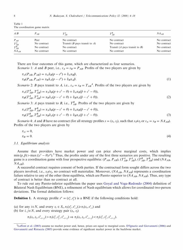
interested in a transit agreement with player j, where i is the generator and j is the receiver. si ¼ NAij indicatesthat provider i is not interested in any form of contract with player j. The outcomes of possible combinationsof the decisions are given in Table 1.

Under the peering agreement i bears per unit transport cost, 0ocpp1, on the traffic coming from j, while j

bears per unit transport cost, cp, on the traffic coming from i. This is a consequence of so-called ‘‘hot-potatorouting’’. The providers pass on off-net traffic as soon as possible, and as a result, most of the transportingcost is borne by the receiving provider. On the other hand, when i pays transit to j, then i pays per unit price0octp1, for the traffic both to and from j. At the same time, under the transit relationship, if i pays transit toj, then i receives positive benefit for the whole traffic exchanged, while j incurs negative benefit from the wholetraffic exchanged.

ARTICLE IN PRESS

Table 1

The coordination game matrix

A/B PAB TAAB TB

ABNAAB

PAB Peer No contract No contract No contract

TAAB

No contract Transit (B pays transit to A) No contract No contract

TBAB

No contract No contract Transit (A pays transit to B) No contract

NAAB No contract No contract No contract No contract

N. Badasyan, S. Chakrabarti / Telecommunications Policy 32 (2008) 4–188

There are four outcomes of this game, which are characterized as four scenarios.Scenario 1: A and B peer, i.e., sA ¼ sB ¼ PAB. Profits of the two players are given by

pAðPAB;PABÞ ¼ aA ~aBðp� cpÞ þ ~aAaB ~p,

pBðPAB;PABÞ ¼ aB ~aAðp� cpÞ þ ~aBaA ~p. ð1Þ

Scenario 2: B pays transit to A, i.e., sA ¼ sB ¼ TABA. Profits of the two players are given by

pAðTAAB;T

AABÞ ¼ aA ~aBðpþ ct � yÞ þ ~aAaBð ~pþ ct � yÞÞ,

pBðTAAB;T

AABÞ ¼ aB ~aAðp� ct þ yÞ þ ~aBaAð ~p� ct þ yÞÞ. ð2Þ

Scenario 3: A pays transit to B, i.e., TBAB. Profits of the two players are given by

pAðTBAB;T

BABÞ ¼ aA ~aBðp� ct þ yÞ þ ~aAaBð ~p� ct þ yÞÞ,

pBðTBAB;T

BABÞ ¼ aB ~aAðpþ ct � yÞ þ ~aBaAð ~pþ ct � yÞÞ. ð3Þ

Scenario 4: A and B have no contract (for all strategy profiles s ¼ (si, sj), such that si 6¼sj or sA ¼ sB ¼ NAAB).Profits of the two players are given by

pA ¼ 0,

pB ¼ 0. ð4Þ

3.1. Equilibrium analysis

Assume that providers have market power and can price above marginal costs, which impliesmin ðp; ~pÞ4max ðjct � yjcpÞ.3 Thus, the profits under any of the first three scenarios are positive. The resultinggame is a coordination game with four prospective equilibria: (PAB, PAB), ðT

AAB;T

AABÞ, ðT

BAB;T

BABÞ and (NAAB,

NAAB).A successful contract requires consent of both parties. If the contractual form sought differs across the two

players involved, i.e., si 6¼sj, no contract will materialize. Moreover, (NAAB, NAAB) represents a coordinationfailure relative to any of the other three equilibria, which are Pareto superior to (NAAB, NAAB). Thus, any typeof contract is better than no contract at all.

To rule out any Pareto-inferior equilibrium the paper uses Goyal and Vega-Redondo (2004) definition ofBilateral Nash Equilibrium (BNE), a refinement of Nash equilibrium which allows for coordinated two-persondeviations. The formal definition follows:

Definition 1. A strategy profile s� ¼ ðs�i ; s�j Þ is a BNE if the following conditions hold:

(a)

3L

Gio

for any iAN, and every si 2 Si;piðs�i ; s��iÞXpiðsi; s��iÞ and

(b)

for i, jAN, and every strategy pair (si, sj)

piðsi; sj ; s��i�jÞ4piðs

�i ; s�j ; s��i�jÞ ) pjðsi; sj ; s

��i�jÞopjðs

�i ; s�j ; s��i�jÞ.

affont et al. (2003) assume no market power and, hence, prices are equal to marginal costs. D’Ignazio and Giovannetti (2006) and

vannetti and Ristuccia (2005) provide some evidence of significant market power in the backbone market.

ARTICLE IN PRESSN. Badasyan, S. Chakrabarti / Telecommunications Policy 32 (2008) 4–18 9

In other words, at the equilibrium, no player or a pair of players can deviate and benefit from thedeviation. Thus, Scenario 4 can be ruled out as a BNE.

Denote RA to be the proportion of the total traffic coming to A from B, and RB to be the proportion of thetotal traffic coming to B from A, i.e.

RA ¼aA ~aB

aA ~aB þ ~aAaB

,

RB ¼aB ~aA

aB ~aA þ ~aBaA

. ð5Þ

Note that RA+RB ¼ 1. Further let k�i

l denote the fact that player i has a strictly higher profit from scenario k

compared to scenario l.

Proposition 1. Peering is BNE if and only if maxðRA;RBÞojðy� ctÞ=cpj and jðy� ctÞ=cpjX1=2. Transit is

always an equilibrium outcome.

The proof of Proposition 1 is provided in Appendix A.Another consequence of the current routing protocols is that peering imposes a net cost on the provider i

amounting to cpRiT , where T ¼ aA ~aB þ ~aAaB is the total traffic flow. Under transit, however, there are no netcosts since it simply results in a transfer of jy� ctjT from one provider to the other. So while the joint profitsare pA þ pB ¼ ðpþ ~pÞT under transit, they are pA þ pB ¼ ðpþ ~p� cpÞT under peering. This directly leads tothe following proposition.

Proposition 2. The joint profits are maximized under a transit agreement.

3.2. The game with transfer arrangements

The analysis in the previous section suggests that any type of connection is better than no connection at all.On the other hand, if the traffic imbalances are large, peering is not a BNE, and transit is preferred. Peering isBNE, if and only if the traffic imbalances are small across the providers and jðy� ctÞ=cpjX1=2. Thus, theproviders will always choose either transit or peering, and unless the traffic imbalances are small, transit isalways preferred. To capture this and also the type of transit that is more likely to be chosen by the providers,this section redefines the game with only peering and transit strategy choices. The providers have incentive toreach a transit agreement, and if they do not manage to coordinate their transit choices, they will peer.

In the game the providers simultaneously announce a transfer arrangement (Bloch & Jackson, 2007). Thetransfer choice of a provider shows whether the provider is willing to pay for the traffic exchanged or demandthe other party to pay for it. Let ti represent i’s transfer decision on the connection between i and j, wherei,jA{A, B}

ti ¼�1 if i demands j to pay for the traffic exchanged;

1 if i offers j to pay for the traffic exchanged:

(

Let g determine the peering/transit agreement resulting from the transfer arrangement choices of theproviders, i.e.

g ¼0 for transit;

1 for peering:

(

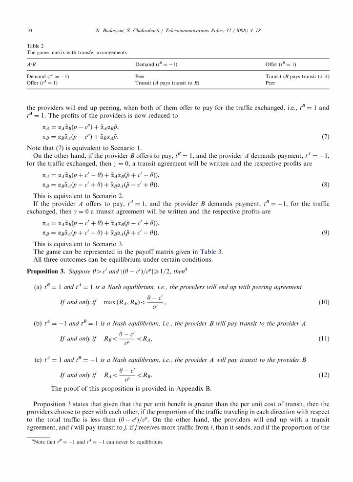
The outcomes of possible combinations of the decisions are given in Table 2.The profit of i from its connection with j, where, i 6¼j and i, jA{A, B}, is now given by

pi ¼ ai ~ajðp� gcp � tið1� gÞðct � yÞÞ þ ~aiajð ~p� tið1� gÞðct � yÞÞ. (6)

There are three possible outcomes of the game. When both providers demand payments for the trafficexchanged, i.e., tB

¼ �1 and tA¼ �1, then g ¼ 1 and the providers end up with peering agreement. Similarly,

ARTICLE IN PRESS

Table 2

The game matrix with transfer arrangements

A/B Demand (tB¼ �1) Offer (tB

¼ 1)

Demand (tA¼ �1) Peer Transit (B pays transit to A)

Offer (tA¼ 1) Transit (A pays transit to B) Peer

N. Badasyan, S. Chakrabarti / Telecommunications Policy 32 (2008) 4–1810

the providers will end up peering, when both of them offer to pay for the traffic exchanged, i.e., tB¼ 1 and

tA¼ 1. The profits of the providers is now reduced to

pA ¼ aA ~aBðp� cpÞ þ ~aAaB ~p,

pB ¼ aB ~aAðp� cpÞ þ ~aBaA ~p. ð7Þ

Note that (7) is equivalent to Scenario 1.On the other hand, if the provider B offers to pay, tB

¼ 1, and the provider A demands payment, tA¼ �1,

for the traffic exchanged, then g ¼ 0, a transit agreement will be written and the respective profits are

pA ¼ aA ~aBðpþ ct � yÞ þ ~aAaBð ~pþ ct � yÞÞ,

pB ¼ aB ~aAðp� ct þ yÞ þ ~aBaAð ~p� ct þ yÞÞ. ð8Þ

This is equivalent to Scenario 2.If the provider A offers to pay, tA

¼ 1, and the provider B demands payment, tB¼ �1, for the traffic

exchanged, then g ¼ 0 a transit agreement will be written and the respective profits are

pA ¼ aA ~aBðp� ct þ yÞ þ ~aAaBð ~p� ct þ yÞÞ,

pB ¼ aB ~aAðpþ ct � yÞ þ ~aBaAð ~pþ ct � yÞÞ. ð9Þ

This is equivalent to Scenario 3.The game can be represented in the payoff matrix given in Table 3.All three outcomes can be equilibrium under certain conditions.

Proposition 3. Suppose y4ct and jðy� ctÞ=cpjX1=2, then4

(a)

4Not

tB¼ 1 and tA

¼ 1 is a Nash equilibrium, i.e., the providers will end up with peering agreement

If and only if max ðRA;RBÞoy� ct

cp, (10)

(b)

tA¼ �1 and tB

¼ 1 is a Nash equilibrium, i.e., the provider B will pay transit to the provider A

If and only if RBoy� ct

cpoRA, (11)

(c)

tA¼ 1 and tB

¼ �1 is a Nash equilibrium, i.e., the provider A will pay transit to the provider B

If and only if RAoy� ct

cpoRB. (12)

The proof of this proposition is provided in Appendix B.

Proposition 3 states that given that the per unit benefit is greater than the per unit cost of transit, then theproviders choose to peer with each other, if the proportion of the traffic traveling in each direction with respectto the total traffic is less than ðy� ctÞ=cp. On the other hand, the providers will end up with a transitagreement, and i will pay transit to j, if j receives more traffic from i, than it sends, and if the proportion of the

e that tB¼ �1 and tA

¼ �1 can never be equilibrium.

ARTICLE IN PRESS

D

E

RB

RA

(θ-ct)/cp

(θ-ct)/cp

1

1

C

F

Fig. 1. The constraints under Proposition 3.

Table 3

The payoff matrix of the game with transfer arrangements

A/B �1 1

�1 pA ¼ aA ~aBðp� cpÞ þ ~aAaB ~p

pB ¼ aB ~aAðp� cpÞ þ ~aBaA ~p

pA ¼ aA ~aBðpþ ct � yÞ þ ~aAaBð ~pþ ct � yÞÞ

pB ¼ aB ~aAðp� ct þ yÞ þ ~aBaAð ~p� ct þ yÞÞ

1 pA ¼ aA ~aBðp� ct þ yÞ þ ~aAaBð ~p� ct þ yÞÞ

pB ¼ aB ~aAðpþ ct � yÞ þ ~aBaAð ~pþ ct � yÞÞ

pA ¼ aA ~aBðp� cpÞ þ ~aAaB ~p

pB ¼ aB ~aAðp� cpÞ þ ~aBaA ~p

N. Badasyan, S. Chakrabarti / Telecommunications Policy 32 (2008) 4–18 11

traffic received by j with respect to the total traffic is greater than ðy� ctÞ=cp, while the proportion of the trafficsend to i with respect to the total traffic is less than ðy� ctÞ=cp, where i, jA{A, B}, and i6¼j.

Then, if ðy� ctÞ=cpo1, Proposition 3 can be summarized in Fig. 1. DE shows all the combinations of RA

and RB, where condition (10) holds. Thus, for all combination of RA and RB on DE the providers will end upwith a peering agreement. Similarly, EF and CD show, the combinations of RA and RB, where conditions (11)and (12) hold, respectively, and the providers end up with a transit agreement.

Proposition 4. Suppose yoct and jðy� ctÞ=cpjX1=2, then

(a)

tBAB ¼ �1 and tA

AB ¼ �1 is a Nash equilibrium, i.e., the providers will end up with peering agreement

If and only if max ðRA;RBÞoct � y

cp, (13)

(b)

tAAB ¼ �1 and tB

AB ¼ 1 is a Nash equilibrium, i.e., the provider B will pay transit to the provider A

If and only if RBoct � y

cpoRA, (14)

(c)

tAAB ¼ 1 and tB

AB ¼ �1 is a Nash equilibrium, i.e., the provider A will pay transit to the provider B

If and only if RAoct � y

cpoRB. (15)

ARTICLE IN PRESS

D

E

RB

RA

(ct-θ)/cpp

(ct-θ)/cpp

1

1

C

F

Fig. 2. The constraints under Proposition 4.

N. Badasyan, S. Chakrabarti / Telecommunications Policy 32 (2008) 4–1812

Proof. The proof is analogous to that of Proposition 3. &

Proposition 4 states that given that the per unit benefit is less than the per unit cost of transit, the providerschoose to peer with each other, if the proportion of the traffic traveling in each direction with respect to thetotal traffic is less than (ct

�y)/cp. On the other hand, the providers end up with a transit agreement, and i willpay transit to j, if j receives more traffic from i, than it sends, and if the proportion of traffic received by j withrespect to the total traffic is more than (ct

�y)/cp, while the proportion of traffic send to i with respect to thetotal traffic is less than (ct

�y)/cp, where i, jA{A, B}, and i 6¼j.

If ðct � yÞ=cpo1, then the constraints under Proposition 4 can be summarized in Fig. 2. DE shows all thecombinations of RA and RB, where condition (13) holds. Thus, for all combination of RA and RB on DE theproviders will end up with a peering agreement. Similarly, EF and CD show, the combinations of RA and RB,where conditions (14) and (15) hold, respectively, and the providers end up with a transit agreement. Again,the joint profits are maximized under a transit agreement.

Thus, given the providers network characteristics, customers’ characteristics, as well as costs and the pricescharged to customers, the model provides conditions that determine the peering/transit decisions of theproviders.

Corollary 1. The outcome yielding the maximum joint profit coincides with the Nash equilibrium if any ofthese conditions hold.

ðaÞ y4ct andy� ct

cpX

1

2and RAo

y� ct

cpoRB or

ðbÞ y4ct andy� ct

cpX

1

2and RBo

y� ct

cpoRA or

ðcÞ yoct andct � y

cpX

1

2and RBo

ct � ycp

oRA or

ðdÞ yoct andct � y

cpX

1

2and RAo

ct � ycp

oRB.

Thus, if there is a large traffic imbalance between two providers, a transit arrangement is a Nash equilibrium,and the joint profits are maximized.

4. Extensions

In this section, some of the assumptions of the earlier sections are relaxed and extended in the model.Firstly, assume that cp represents the average cost of peering and is different among the providers withdifferent traffic flows. The cost of peering at an exchange point includes fixed costs of the equipment and the

ARTICLE IN PRESSN. Badasyan, S. Chakrabarti / Telecommunications Policy 32 (2008) 4–18 13

transmission capacity, and variable costs of transporting traffic received from the peering partner. As moretraffic is exchanged, the average fixed cost per Mbps, AFCiðai ~aj ; ~aiajÞ, falls. On the other hand, when traffic ishanded over from provider j to provider i, the latter incurs a transport cost. As a result of ‘‘hot-potatorouting’’, the more traffic is sent by j’s websites, the higher is the transport cost incurred by i. Further, assumethe average (variable) transport cost, AFCiðai ~ajÞ, is increasing in ai ~aj.

Then, the average cost per unit incurred by i, under the peering agreement would be

cpi ðai ~aj ; ~aiajÞ ¼ AFCiðai ~aj ; ~aiajÞ þ AVCiðai ~ajÞ.

Note that ðqcpi Þ=ðq ~aiajÞo0, i.e. the more traffic i sends to j, the smaller is its average cost per unit of peering.

When the total traffic exchanged is small, then fixed costs are visibly large relative to variable transport costs,so that the reduction in average fixed costs from increasing traffic received from j dominates the rise in averagetransport costs, thus, ci

p is decreasing in ai ~aj. On the other hand, when the total traffic exchanged is very largedue to the received traffic from j, then the reduction in average fixed costs from increasing traffic becomes lessrelative to the increase in average transport costs, thus ci

p is increasing in ai ~aj, after certain ðai ~ajÞ�. Tiers-1

and -2 providers generally exchange a large amount of traffic, thus, assume ðqcpi Þ=ðqai ~ajÞ40 The average

per unit cost of peering are cpAðaA ~aB; ~aAaBÞ for provider A and c

pBðaA ~aB; ~aAaBÞ for provider B, such that

ðqcpAÞ=ðqaA ~aBÞ40 and ðqc

pBÞ=ðq ~aAaBÞ40. If market shares and therefore traffic flows are exogenous, the

average costs of peering are exogenous as well. Moreover, RA4RB implies cpA4c

pB, while RAoRB implies

cpAoc

pB.

The profit of i from its connection with j, where, i 6¼j and i, jA{A, B}, is now given by

pi ¼ ai ~ajðp� gcpi � tið1� gÞðct � yÞÞ þ ~aiajð ~p� tið1� gÞðct � yÞÞ.

Then the profits under Scenario 1 now are given by

pAðPAB;PABÞ ¼ aA ~aBðp� cpAÞ þ ~aAaB ~p,

pBðPAB;PABÞ ¼ aB ~aAðp� cpBÞ þ ~aBaA ~p

while the profits under other scenarios remain as above.The game with transfer arrangements is represented in the payoff matrix given in Table 4.There are three possible outcomes of the game: A and B peer, A is the receiver and B is the generator in a

transit agreement, and A is the generator and B is the receiver in a transit agreement. All three outcome can beequilibrium under certain conditions.

Proposition 5. Suppose y4ct and min ðy� ct=cpA; Þ=ðy� ctÞ=c

pBX1=2, then

(a)

Tab

The

A/B

�1

1

tB¼ 1 and tA

¼ 1 is a Nash equilibrium, i.e., the providers will end up with peering agreement

If and only if max ðRA;RBÞominy� ct

cpA

;y� ct

cpB

� �,

le 4

payoff matrix of the game with non-linear peering costs

�1 1

pA ¼ aA ~aBðp� cpAÞ þ ~aAaB ~p,

pB ¼ aB ~aAðp� cpBÞ þ ~aBaA ~p

pA ¼ aA ~aBðpþ ct � yÞ þ ~aAaBð ~pþ ct � yÞÞ,

pB ¼ aB ~aAðp� ct þ yÞ þ ~aBaAð ~p� ct þ yÞÞ

pA ¼ aA ~aBðp� ct þ yÞ þ ~aAaBð ~p� ct þ yÞÞ,

pB ¼ aB ~aAðpþ ct � yÞ þ ~aBaAð ~pþ ct � yÞÞ

pA ¼ aA ~aBðp� cpAÞ þ ~aAaB ~p

pB ¼ aB ~aAðp� cpBÞ þ ~aBaA ~p

ARTICLE IN PRESSN. Badasyan, S. Chakrabarti / Telecommunications Policy 32 (2008) 4–1814

(b)

tA¼ �1 and tB

¼ 1 is a Nash equilibrium, i.e., the provider B will pay transit to the provider A, if and only if

any of the following holds

RBoy� ct

cpA

oy� ct

cpB

oRA

or

RBoy� ct

cpA

oRAoy� ct

cpB

,

(c)

tA¼ 1 and tB

¼ �1 is a Nash equilibrium, i.e., the provider A will pay transit to the provider B, if and only if

any of the following holds

RAoy� ct

cpB

oy� ct

cpA

oRB

or

RAoy� ct

cpB

oRBoy� ct

cpA

.

Proof. The proof is analogous to that of Proposition 3. &

On the other hand, if yoct Proposition 6 follows:

Proposition 6. Suppose yoct and min ðct � y=cpA; c

t � y=cpBÞX1=2, then

(a)

tBAB ¼ �1 and tA

AB ¼ �1 is a Nash equilibrium, i.e., the providers will end up with peering agreement, if and

only if

max ðRA;RBÞominct � y

cpA

;ct � y

cpB

� �,

(b)

tAAB ¼ �1 and tB

AB ¼ 1 is a Nash equilibrium, i.e., the provider B will pay transit to the provider A, if and

only if

RBoct � y

cpA

oct � y

cpB

oRA

or

RBoct � y

cpA

oRAoct � y

cpB

,

(c)

tAAB ¼ 1 and tB

AB ¼ �1 is a Nash equilibrium, i.e., the provider A will pay transit to the provider B, if and

only if

RAoct � y

cpB

oct � y

cpA

oRB

or

RAoct � y

cpB

oRBoct � y

cpA

.

Proof. The proof is analogous to that of Proposition 3. &

If jy� ct=cpAjo1 and jy� ct=c

pBjo1, the constraints under Propositions 5 and 6 can be presented in Fig. 3.

ARTICLE IN PRESS

Fig. 3. The constraints under Propositions 5 and 6.

N. Badasyan, S. Chakrabarti / Telecommunications Policy 32 (2008) 4–18 15

DE shows all the combinations of RA and RB, where providers peer. EF shows all the combinations of RA

and RB, where the conditions of parts (b) of Propositions 5 and 6 hold, thus B pays transit to A. CD shows thearea where the conditions of parts (c) of Propositions 5 and 6 hold. Thus, A pays transit to B.

Under the transit agreement, if one provider charges transit to the other one, then the latter pays for thetraffic in both directions. Transit charges are usually levied on the basis of per unit of traffic and remainconstant over a certain range, but tend to come down in a step-wise manner as traffic volume increases(Norton, 2002). Assume ctðTÞ40 (transit charge per Mbps) is the average unit price of transit and it decreasesas the total volume of traffic (transit commit) increases, ðdct=dTÞo0: On the other hand, assume y is afunction of the total traffic handled under the transit agreement and represents both the additional benefitreceived by generator and an additional cost imposed on the receiver on the per unit traffic exchanged. Furtherassume ðdy=dTÞ40, i.e., the more traffic is exchanged, the larger is the additional per unit cost y (additionaldelay and packet loss) imposed on the receiver (similarly, the more traffic is exchanged, the larger is theadditional per unit benefit received by the generator). If the amount of traffic exchanged among the providersis large enough, as it is the case with Tiers-1 and -2 providers, then y4ct will hold. Thus, the assumptions ofProposition 5 will hold. Note that the assumption of y4ct under part (b) in Proposition 5 implies that B (theprovider that sends much more traffic than receives) prefers paying transit to peering. On the other hand,ðy� ct=c

pAÞoRA implies that A (the provider that receives much more traffic than sends) prefers to be paid for

the traffic exchanged rather than peer. This suggests that there are competitive reasons for choosing transitover peering, when traffic imbalances are large.

5. Conclusions

As interconnection arrangements currently are not subject to regulation, policymakers are concerned aboutpossible anti-competitive behavior of large providers. Increasing transparency in peering requirements in pastyears was Tier-1 providers’ likely attempt to ‘‘(i) avoid government regulation, (ii) preempt anti-trustaccusations, and (iii) meet the standard of transparency set by the industry newcomers’’ (McGarty, 2002).Many of the published peering requirements state that the traffic ratio under peering agreement should beroughly symmetrical (Qwest, 2007; Verizon, 2007). Peering partners do not get any compensation for carryingeach other’s traffic, while incurring costs of transporting each other’s traffic. The costs could be due to the typeof customers that the providers have and/or geographic coverage. Thus, the provider, who carries a lot moretraffic than its partner under peering agreement, has a valid competitive reason to deny peering. The purposeof this paper was to develop a simple theoretical framework for modeling the peering/transit decisions ofTiers-1 and -2 providers taking into account traffic flows. Providers balance the benefits against the costs todetermine whether to peer or transit. In general, this balance takes into account traffic volume, customer base(including customer loyalty, size, and demographics), the range of different services offered, the quality ofonward connectivity and technology used (Lie, 2007). Many models discussed earlier in this paper examinestrategic elements behind the interconnection decisions focusing on business stealing and network externality

ARTICLE IN PRESSN. Badasyan, S. Chakrabarti / Telecommunications Policy 32 (2008) 4–1816

effects. The approach in this paper is based on the cost aspects of interconnection incentives resulting fromtraffic imbalances. Even though the traffic imbalance is not the only factor determining the relative benefitsand costs of interconnection, it is still a major factor in determining the peering. To account for the customerbase, the paper considers two types of customers (websites and consumers) who are charged the same pricesfor the similar services regardless of the provider to which they are connected. The model discusses a set ofconditions, which determine the formation of peering and transit agreements. The providers weigh the benefitsand costs of entering into a particular interconnection agreement. The decisions are based on how one variableweighs against the other. One provider may demand a transit arrangement, if it believes that the otherprovider might free ride on its infrastructure investments, because the former might be the one transportingmost of the traffic between them. On the other hand, a provider might be better off with a transit agreement,as it can dump more traffic on the transit seller, than it could under the peering agreement. In addition, as longas there are several Tier-1 providers of roughly comparable size, there are enough incentives to offerreasonable prices for transit and enhance the connectivity. Indeed, the prices of transit have droppedsubstantially (TeleGeography, 2004). When a provider carrying most of the traffic under the peeringarrangements terminates the peering agreement and demands transit, it is not necessarily driven by anti-competitive motives, as it will not be able to easily manipulate transit prices to gain competitive advantage.Since one provider incurs most of the transporting costs under the peering agreement due to trafficimbalances, it has a valid competitive reason to refuse peering. Moreover, the joint profits are maximizedunder the transit arrangement. Under the transit agreement the transit customer pays for the traffic carried bythe transit seller, while getting benefits of dumping most of its traffic on the transit seller. These two effectscancel out when maximizing the joint profits of the transit partners. In addition, the degree of competition islarge in the transit market. Several large providers are competing with each other for transit arrangements. Asa result of competitive pressures, transit prices have dropped steadily and substantially (Lie, 2007) in recentyears. This also suggests that there is no need for regulation targeting transit charges.

Acknowledgments

The authors would like to thank Robert P. Gilles, two anonymous referees and the editor for their veryinsightful comments. The usual disclaimer applies.

Appendix A. Proof of Proposition 1

Suppose y4ct and RBoðy� ctÞ=cpoRA.Given that y4ct, B always prefers Scenario 2 to 1 as well as 2 to 3, i.e.

2�B1 since aB ~aAðp� ct þ yÞ þ ~aBaAð ~p� ct þ yÞÞ4aB ~aAðp� cpÞ þ ~aBaA ~p and

2�B3 since aB ~aAðp� ct þ yÞ þ ~aBaAð ~p� ct þ yÞÞ4aB ~aAðpþ ct � yÞ þ ~aBaAð ~pþ ct � yÞÞ.

On the other hand RBoðy� ctÞ=cp implies that

aB ~aAðp� cpÞ þ ~aBaA ~p4aB ~aAðpþ ct � yÞ þ ~aBaAð ~pþ ct � yÞÞ; thus 1�B3.

Similarly, y4ct implies that A prefers Scenario 3 to 1 and 3 to 2, i.e.

3�A1 since aA ~aBðp� ct þ yÞ þ ~aAaBð ~p� ct þ yÞÞ4aA ~aBðp� cpÞ þ ~aAaB ~p and

3�A2 since aA ~aBðp� ct þ yÞ þ ~aAaBð ~p� ct þ yÞÞ4aA ~aBðpþ ct � yÞ þ ~aAaBð ~pþ ct � yÞÞ.

On the other hand, ðy� ctÞ=cpoRAimplies that

aA ~aBðpþ ct � yÞ þ ~aAaBð ~pþ ct � yÞÞ4aA ~aBðp� cpÞ þ ~aAaB ~p; thus 2�A1.

Hence, y4ct and RBoðy� ctÞ=cpoRA imply that 2�B1�

B3�

B4 and 3�

A2�

A1�

A4. Since 2�

A1 and 2�

B1,

Scenario 1 (peering) cannot be a BNE. Let us refer to this case as Case 1B. The Tables 5 and 6 below

ARTICLE IN PRESS

Table 5

Case 1: y4ct

Cases Parameter range Preference configuration BNE

Case 1AmaxðRA;RBÞo

y� ct

cp

3�A1�

A2�

A4; 2�

B1�

B3�

B4 1, 2, 3

Case 1BRBo

y� ct

cpoRA

3�A2�

A1�

A4; 2�

B1�

B3�

B4 2,3

Case 1CRAo

y� ct

cpoRB

3�A1�

A2�

A4; 2�

B3�

B1�

B4 2,3

Bilateral Nash equilibria.

Table 6

Case 2: yoct

Case Parameter range Preference configuration BNE

Case 2AmaxðRA;RBÞo

ct � ycp

3�A1�

A2�

A4; 2�

B1�

B3�

B4 1, 2, 3

Case 2BRBo

ct � ycp

oRA

3�A1�

A2�

A4; 2�

B1�

B3�

B4 2,3

Case 2CRAo

ct � ycp

oRB

3�A1�

A2�

A4; 2�

B3�

B1�

B4 2,3

Bilateral Nash equilibria.

N. Badasyan, S. Chakrabarti / Telecommunications Policy 32 (2008) 4–18 17

summarize preference patterns for other parameter constraints. Using a similar logic as above, Scenario 1 isnot a BNE in Cases 1C, 2B and 2C.

Only in Cases 1A and 2A, when max ðRA;RBÞojðy� ctÞ=cpj, 3�A1�

A2�

A4; 2�

B1�

B3�

B4, which implies that

peering is BNE. However, note that if jðy� ctÞ=cpjo1=2, peering can never be BNE. Since RA+RB ¼ 1 bydefinition, then if jðy� ctÞ=cpjo1=2, then the following condition will never hold max ðRA;RBÞojðy� ctÞ=cpj.The other parts of the proposition are summarized in Tables 5 and 6.

This concludes the proof. &

Appendix B. Proof of Proposition 3

Commence with assuming condition (10). Then A’s best response to the given strategy of B, tB¼ 1, is

tA¼ 1, because

aA ~aBðpþ ct � yÞ þ ~aAaBð ~pþ ct � yÞÞoaA ~aBðp� cpÞ þ ~aAaB ~p.

On the other hand, A’s best response to the given strategy of B, tB¼ �1, is tA

¼ 1, because

aA ~aBðp� cpÞ þ ~aAaB ~poaA ~aBðp� ct þ yÞ þ ~aAaBð ~p� ct þ yÞÞ.

Similarly, B’s best response to the given strategy of A, tA¼ 1, is tB

¼ 1, because

aB ~aAðpþ ct � yÞ þ ~aBaAð ~pþ ct � yÞÞoaB ~aAðp� cpÞ þ ~aBaA ~p

and B’s best response to the given strategy of A, tA¼ �1, is tB

¼ 1, because

aB ~aAðp� cpÞ þ ~aBaA ~poaB ~aAðp� ct þ yÞ þ ~aBaAð ~p� ct þ yÞÞ.

The other parts of the proposition follow the same way.

ARTICLE IN PRESSN. Badasyan, S. Chakrabarti / Telecommunications Policy 32 (2008) 4–1818

References

Baake, P., & Wichmann, T. (1999). On the economics of Internet peering. Netnomics, 1(1), 89–105.

Bloch, F., & Jackson, M. (2007). The formation of networks with transfers among players. Journal of Economic Theory, 133(1), 83–110.

Cremer, J., Rey, P., & Tirole, J. (2000). Connectivity in the commercial Internet. The Journal of Industrial Economics, XLVIII(43),

433–472.

D’Ignazio, A., & Giovannetti, E. (2006). Antitrust analysis for the Internet upstream market: A border gateway protocol approach.

Journal of Competition Law and Economics, 2(1), 43–69.

Economides, N. (2006). The economics of the Internet backbone. In S. Majumdar, & I. Vogelsang (Eds.), Handbook of telecommunications

economics, Vol. II (pp. 375–412). Amsterdam: Elsevier Publishers.

Foros, Ø., & Hansen, J. (2001). Competition and compatibility among Internet service providers. Information Economics and Policy, 13,

411–425.

Giovannetti, E., & Ristuccia, C. A. (2005). Estimating market power in the Internet backbone. Using the IP transit Band-X database.

Telecommunications Policy, 29, 269–284.

Goyal, S., & Vega-Redondo, F. (2004). Structural holes in social networks. Mimeo. /http://www2.warwick.ac.uk/fac/soc/economics/

forums/conferences/game_theory/goyal.pdfS.

Greenstein, S. (2000). Building and delivering the virtual world: Commercializing services for Internet access. Journal of Industrial

Economics, 48(4), 391–411.

Honnef, B. (2002). The economics of IP networks—Market, technical and public policy issues relating to Internet traffic exchange. Study

for the European Commission, wik-consult. /http://europa.eu.int/information_society/topics/telecoms/regulatory/studies/documents/

ip_final_report_and_annex_geaendert2.pdfS.

Jahn, E., & Prufer, J. (2004). Transit versus (paid) peering: Interconnection and competition in the Internet backbone market. SSRN working

paper ]590582.Katz, M. L., & Shapiro, C. (1985). Network externalities, competition, and compatibility. The American Economic Review, 75, 424–440.

Kende, M. (2000). The digital handshake: Connecting Internet backbones. OPP working paper no. 32, Federal Communications

Commission, Washington, DC.

Laffont, J. J., Marcus, S., Rey, P., & Tirole, J. (2003). Internet interconnection and the off-net-cost pricing principle. RAND Journal of

Economics, 34(2), 370–390.

Lie, E. (2007). International Internet interconnection next generation networks and development. GSR 2007 discussion paper.

Mackie-Mason, J. K., & Varian, H. R. (1995). Pricing the Internet. In B. Kahin, & J. Keller (Eds.), Public access to the Internet

(pp. 269–314). Cambridge, MA: MIT Press.

Marich, R. (2006). Cable modem vs. DSL: Rivals side-step big price wars so far. Kagan insights, July 06, 2006. Kagan Research.

McGarty, T. (2002). Peering, transit, interconnection: Internet access in Central Europe. ITC working paper. MIT, Cambridge, MA.

Norton, W. (2002). A business case for ISP peering. Equinix White Papers. /http://www.equinix.com/pdf/whitepapers/Business_

case.pdfS.

Peering BOF XI. (2006). North American Network Operators Group.

Prufer, J., & Jahn, E. (2007). Dark clouds over the Internet? Telecommunications Policy, 31(3–4), 144–154.

Qwest. (2007). Qwest’s North America IP network peering policy. June 6, 2007. /http://www.qwest.com/legal/peering_na.htmlS.

Shin, S. J., & Weiss, M. (2004). Internet interconnection economic model and its analysis: Peering and settlement. Netnomics, 6(1), 43–57.

TeleGeography. (2004). Press release September 14, 2004. /http://www.telegeography.com/press/releases/2004-09-14.phpS.

Turner, S.D. (2005). Broadband reality check. Free Press, Consumers Union, The Consumer Federation of America, August 2005. /http://

www.freepress.net/docs/broadband_report.pdfS.

Verizon. (2007). Verizon policy for settlement-free interconnection with Internet networks. /http://biz.verizon.net/policies/peering_

policy.aspS.