a simple cooperative diversity method based on network path...
TRANSCRIPT

A Simple Cooperative Diversity Method Based on
Network Path Selection
Aggelos Bletsas, Ashish Khisti, David P. Reed, Andrew Lippman
Massachusetts Institute of Technology
{aggelos, khisti}@mit.edu
Abstract
Cooperative diversity has been recently shown to provide dramatic gains in slow fading wireless environments.
However most of the proposed solutions require distributed space-time protocols, many of which are infeasible
if there is more than one cooperative relay. We propose a novel scheme, ”opportunistic relaying” that alleviates
these problems and provides diversity gains on the order of the number of relays in the network. Our scheme first
selects the best relay from a set ofM available relays and then uses this ”best” relay for cooperation between the
source and the destination. We develop and analyze a distributed method to select the best relay based on the local
measurements of the channel conditions by the relays. This method also requires no explicit communication among
the relays. The success (or failure) to select the best available path depends on the statistics of the wireless channel,
and a methodology to evaluate performance for any kind of wireless channel statistics, is provided. Information
theoretic analysis of outage probability shows that our scheme achieves the same diversity-multiplexing tradeoff
as achieved by more complex protocols, where coordination and distributed space-time coding for M nodes is
required, such as those proposed in [8]. The simplicity of the technique, allows for immediate implementation in
existing radio hardware and its adoption could provide for improved flexibility, reliability and efficiency in future
4G wireless systems.
I. I NTRODUCTION
In this work, we propose and analyzeOpportunistic Relaying, which is a novel method to select the
”best” end-to-end path between a source and destination of wireless information. The setup includes a
set of cooperating relays which are willing to forward received information towards the destination and
opportunistic relaying is about a distributed algorithm that selects the most appropriate relay to forward
information towards the receiver. The decision is based on the end-to-end instantaneous wireless channel
conditions and the algorithm is distributed among the cooperating wireless terminals.

The best relay selection algorithm lends itself naturally into cooperative diversity protocols, which
have been recently proposed to improve reliability in wireless communication systems using distributed
virtual antennas. The key idea behind these protocols is to create additional paths between the source
and destination terminals using intermediate relay nodes. Reliable communication between the source
and destination is possible ifany one of the paths is strong enough. Several cooperative protocols were
proposed in [7] and their performance was measured in terms of the diversity-multiplexing tradeoff [12].
Their basic setup included one sender, one receiver and one intermediate relay node and both analog as
well as digital processing at the relay node were considered. Subsequently the case when there are several
intermediate relay nodes was considered in [1], [8] and it was shown that the diversity gains achieved are
on the order of the number of relay nodes in the network.
Unfortunately, these protocols require the implementation of distributed space time codes across the
relay nodes and this is practically not feasible: while well known space time codes such as the Alamouti
scheme, can be implemented in the single relay case, to the best of our knowledge, the current state of art
in space time codes is far from developing practical schemes when there is more than one intermediate
relay 1. Apart from practical space-time coding, the formation of virtual antenna arrays using individual
terminals distributed in space, requires significant amount of coordination, which is still an open research
problem. Specifically, the formation of cooperating groups of terminals involves distributed algorithms
[8] while synchronization at the packet level is required among several different transmitters. Those
additional requirements for cooperative diversity demand significant modifications to almost all layers
of the communication stack (up to the routing layer) which has been built according to ”traditional”,
point-to-point (non-cooperative) communication.
In such distributed settings, opportunistic relaying algorithm provides a practical alternative to select
simply the best available relay between the source and the destination rather than involving all available
relays and then using the well known space time protocols used in the single relay case. Additionally, the
algorithm itself provides for the necessary coordination in time and group formation among the cooperating
terminals.
A natural question to consider is how much performance loss is incurred through this practically appeal-
ing alternative as compared to the more complicated protocols. In this work we study this performance loss.
Surprisingly we observe that in terms of the diversity multiplexing tradeoff, there is no performance loss
1At least we are not aware of generalizations of Alamouti scheme that achieve the entire diversity multiplexing tradeoff curve.
2

A
B
Opportunistic Relaying
Space-Time codingfor M relays
Fig. 1. A transmission is overheard by neighboring nodes. Practical cooperative diversity schemes should address which nodes are beneficial
to relay information to the receiver. Distributed Space-Time coding is needed so that all overhearing nodes could simultaneously transmit.
In this work we analyze ”Opportunistic Relaying” where the relay with the strongest transmitter-relay-receiver channel is selected, among
several candidates, in a distributed fashion.
compared to more complicated protocols, such as that proposed in [8]. Intuitively, the gains in cooperative
diversity do not come from using complex schemes, but rather from the fact that we have enough relays
in the system to provide sufficient diversity.
In the following sections, we first explain in detail the motivation behind this work. We then describe the
algorithm and present a simple probabilistic analysis that quantifies the success (or failure) of selecting the
most appropriate path. Given the dependence of the selection scheme on the wireless channel conditions,
performance is evaluated according to the statistics of the wireless channel. The analytical solution applies
for any kind of wireless channel distribution and specific examples on Rayleigh and Ricean fading are
given. We continue with the diversity-multiplexing tradeoff analysis of the proposed scheme. We conclude
this work in the last section.
The simplicity of the technique, allows for immediate implementation in existing radio hardware.
An implementation of the scheme using custom radio hardware is reported in [3], [4]. Its adoption
could provide for improved flexibility (since the technique addresses coordination issues), reliability and
efficiency (since the technique inherently builds upon diversity) in future 4G wireless systems.
II. M OTIVATION
Cooperative diversity in its simplest form of a transmitter, single relay and receiver, involves relaying
of information from a neighboring overhearing node rather than having the initial transmitter repeat
3

its transmission. The receiver would exploit both direct and relayed transmission over two statistically
independent paths and therefore resistance to fading would improve because of diversity.
In figure 1 a transmitter transmits its information towards the receiver while all the neighboring nodes
are in listening mode. For a practical cooperative diversity in a three-node setup, the transmitter should
know that allowing a relay at location (B) to relay information, would be more efficient than repetition
from the transmitter itself. This is not a trivial task and such event depends on the wireless channel
conditions between transmitter and receiver as well as between transmitter-relay and relay-receiver. What
if the relay is located in position (A)? And how could cooperative diversity scale in practice when larger
number of relays are used?
Current proposals allow for all overhearing nodes to relay simultaneously during the second step of
the scheme (figure 1). Opportunistic relaying needs only two transmissions, one from source and one
from ”best” relay. Therefore, opportunistic relaying simplifies and address cooperative communication
as a Routing problem: how could the best end-to-end path be selected in a distributed and dynamic
way that adapts to the wireless channel conditions? This perspective motivated our work and allowed
the implementation of a demonstration on cooperative diversity, using opportunistic relaying and custom
radio hardware [3], [4].
MIMO theory suggests that selection diversity in a multi-antenna transceiver (i.e. selecting the antenna
with the highest SNR among M antennas) provides for a diversity gain of M, even though one antenna is
used [9]. Therefore, it was natural to explore ”virtual” antenna arrays with the same behavior. Opportunistic
relaying is based on similar ideas and provides for diversity gain equal to the number of cooperating nodes,
even though only two nodes transmit.
III. D ESCRIPTION OFOPPORTUNISTICRELAYING
According to opportunistic relaying, a single relay among a set ofM nodes is selected, depending on
which relay provides for the ”best” end-to-end path between source and destination (figure 1, 2). The
wireless channelasi between source and each relayi, as well as the channelaid between relayi and
destination affect performance. Since communication among all relays should be minimized for reduced
overall overhead, a method based on time was selected: each relay starts a timer from a parameterhi
based on the channel conditionsasi, aid. The timer of the relay with the best end-to-end channel conditions
will expire first. All relays, while waiting for their timer to reduce to zero (i.e. to expire) are in listening
mode. As soon as they hear another relay to forward information (the best relay), they back off.
4

best path @ kT
best path @ (k+1)T
Direct Relayed
|as,j|2 |aj,d|2
Source Destination
Fig. 2. Source transmits to destination and neighboring nodes overhear the communication. The ”best” relay among M candidates is selected
to relay information, via a distributed mechanism and based on instantaneous end-to-end channel conditions.
For the case where all relays can listen source and destination, but they are ”hidden” from each other
(i.e. they can not listen each other), the best relay could notify the destination with a short durationflag
packet and the destination could then notify all relays with a short broadcast message.
All the above assume that all relays start their timers at the same time. Synchronization can be easily
achieved by the exchange of Ready-to-Send (RTS) and Clear-to-Send (CTS) packets between source
and destination. Relays can start their timers as soon as they receive the CTS packet. In that case,
synchronization error on the order of propagation delay differences across all destination-relay pairs should
be taken into account. For the cases where source and destination are not in direct range, they need to
synchronize their RTS/CTS exchange by other means. For example, Network Time Keeping algorithms
in client/server setups, such as those examined in [2] could be employed. Or fully decentralized solutions
for network time keeping could be facilitated, such as those demonstrated in [5].
The RTS/CTS mechanism, existent in most MAC protocols, is also necessary for channel estimation
at the relays: the transmission of RTS from the source allows for the estimation of the wireless channel
asi between source and relayi, at each relayi. Similarly, the transmission of CTS from the destination,
allows for the estimation of the wireless channelaid between relayi and destination, at each relayi,
according to the reciprocity theorem.
The channel estimatesasi, aid at each relay, describe the quality of the wireless path source-relay-
destination, for each relayi. Opportunistic relaying is about selecting the ”best” path amongM possible
5
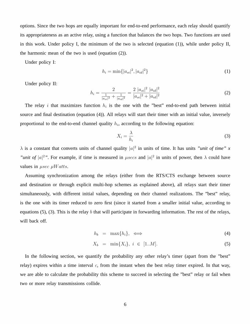
options. Since the two hops are equally important for end-to-end performance, each relay should quantify
its appropriateness as an active relay, using a function that balances the two hops. Two functions are used
in this work. Under policy I, the minimum of the two is selected (equation (1)), while under policy II,
the harmonic mean of the two is used (equation (2)).
Under policy I:
hi = min{|asi|2, |aid|2} (1)
Under policy II:
hi =2
1|asi|2 + 1
|aid|2=
2 |asi|2 |aid|2
|asi|2 + |aid|2(2)
The relay i that maximizes functionhi is the one with the ”best” end-to-end path between initial
source and final destination (equation (4)). All relays will start their timer with an initial value, inversely
proportional to the end-to-end channel qualityhi, according to the following equation:
Xi =λ
hi(3)
λ is a constant that converts units of channel quality|a|2 in units of time. It has units”unit of time” x
”unit of |a|2” . For example, if time is measured inµsecs and |a|2 in units of power, thenλ could have
values inµsec µWatts.
Assuming synchronization among the relays (either from the RTS/CTS exchange between source
and destination or through explicit multi-hop schemes as explained above), all relays start their timer
simultaneously, with different initial values, depending on their channel realizations. The ”best” relay,
is the one with its timer reduced to zero first (since it started from a smaller initial value, according to
equations (5), (3). This is the relayb that will participate in forwarding information. The rest of the relays,
will back off.
hb = max{hi}, ⇐⇒ (4)
Xb = min{Xi}, i ∈ [1..M ]. (5)
In the following section, we quantify the probability any other relay’s timer (apart from the ”best”
relay) expires within a time intervalc, from the instant when the best relay timer expired. In that way,
we are able to calculate the probability this scheme to succeed in selecting the ”best” relay or fail when
two or more relay transmissions collide.
6
As can be seen from the above equations, the scheme depends on the instantaneous channel realizations
or equivalently, on received SNRs. Therefore, the best relay selection algorithm should be applied as often
as the wireless channel changes and not as often the source transmits information. That rate of wireless
channel change depends on thecoherence timeof the channel. The advantage of opportunistic relaying
is that it requires no explicit communication among the relays.
In the following section we will calculate the probability of successful relay selection, even at the case
where the relays are hidden from each other.
IV. PROBABILISTIC ANALYSIS OF OPPORTUNISTICRELAYING
The probability of having two or more relay timers expire ”at the same time” is zero. However, the
probability of having two or more relay timers expire within the same time intervalc is non zero and can
be analytically evaluated, given knowledge of the wireless channel statistics.
The only case where opportunistic relay selections fails, is when the relays cannot listen each other
and therefore, one relay can not detect that another relay is more appropriate for information forwarding.
Note that we have already assumed that all relays can listen initial source and destination, otherwise they
do not participate in the scheme. We will assume two extreme cases: a) all relays can listen to each other
b) all relays are hidden from each other (but they can listen source and destination). In the second case,
the best relay sends a flag packet to destination (or source) to notify for its candidacy, as the best relay.
Then the destination (or source) notifies all relay nodes with a short broadcast message.
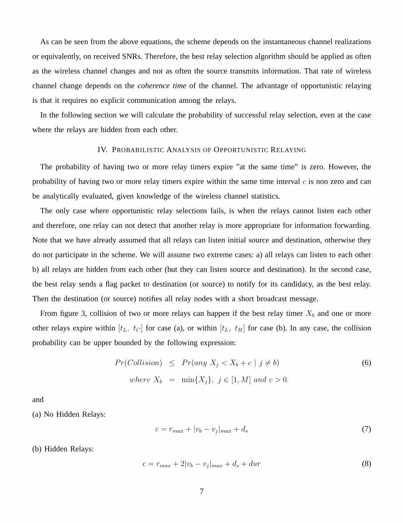
From figure 3, collision of two or more relays can happen if the best relay timerXb and one or more
other relays expire within[tL, tC ] for case (a), or within[tL, tH ] for case (b). In any case, the collision
probability can be upper bounded by the following expression:
Pr(Collision) ≤ Pr(any Xj < Xb + c | j 6= b) (6)
where Xb = min{Xj}, j ∈ [1,M ] and c > 0.
and
(a) No Hidden Relays:
c = rmax + |vb − vj|max + ds (7)
(b) Hidden Relays:
c = rmax + 2|vb − vj|max + ds + dur (8)
7

tL tHtC
Xb ds
dur
tb
tj
dv
r r dv
CTS
CTS
CTS
packet b
Fig. 3. The middle raw corresponds to the ”best” relay. Other relays (top or bottom raw) could erroneously be selected as ”best” relays,
if their timer expired within intervals when they can not hear the best relay transmission. That can happen in the interval[tL, tC ] for case
(a) (No Hidden Relays) or[tL, tH ] for case (b) (Hidden Relays).tb, tj are time points where reception of the CTS packet is completed at
best relayb and relayj respectively.
• vj: propagation delay between relayj and destination.
• rmax: maximum propagation delay between two relays.
• ds: receive-to-transmit switch time of each radio.
• dur: duration of flag packet, transmitted by ”best” relay.
The upper bound of (6) and equations (7), (8) can be easily derived taking into account propagation
delays, radio switch time and flag packet duration.
In the following section, we will provide an analytic way to calculate the upper bound of equation (6).
But before doing so, we will easily show that this probability can be made arbitrary small, close to zero.
If Xb = min{Xj}, j ∈ [1,M ] and Y1 < Y2 < . . . < YM the ordered random variables{Xj} with
Xb ≡ Y1, then:
Pr(any Xj < Xb + c | j 6= b) = Pr(Y2 < Y1 + c) (9)
Given thatYj = λ/h(j), Y1 < Y2 < . . . < YM is equivalent to1/h(1) < 1/h(2) < . . . < 1/h(M), equation
(9) is equivalent to
Pr(Y2 < Y1 + c) = Pr(1
h(2)
<1
h(1)
+c
λ) (10)
andY1 < Y2 < . . . < YM ⇔ h(1) > h(2) . . . > h(M) (h, λ, c are positive numbers).
From the last equation (10), it is obvious that increasingλ at each relay (in equation (3)), reduces the
probability of collision to zero since the upper bound of (10) goes to zero with increasingλ.
8

In practice,λ can not be made arbitrarily large, since it also ”regulates” the expected time, needed for
the network to find out the ”best” relay. From equation (3) and Jensen’s inequality we can see that
E[Xj] = E[λ/hj] ≥ λ/E[hj] (11)
or in other words, the expected time needed for each relay to flag its presence, is lower bounded by
λ. Therefore, there is a trade-off between probability of collision and speed of relay selection. We need
to haveλ as big as possible to reduce collision probability and at the same time, as small as possible,
to quickly select the best relay, before the channel changes again (i.e. within the coherence time of the
channel).
In the following section we provide a method to quantify performance for any kind of wireless channel
statistics and any kind of values forc andλ and show that the scheme can perform reasonably well.
A. CalculatingPr(Y2 < Y1 + c)
Theorem 1:The joint probability density function of the minimum and second minimum amongM i.i.d.
positive random variablesX1, X2, . . . , XM , each with probability density functionf(x) and cumulative
distribution functionF (x), is given by the following equation:
fY1,Y2(y1, y2) = M (M − 1) f(y1) f(y2) [1− F (y2)]M−2
0 < y1 < y2,
fY1 Y2(y1, y2) = 0
elsewhere. (12)
whereY1 < Y2 < Y3 . . . < YM are theM ordered random variablesX1, X2, . . . , XM .
Proof:
Please refer to appendix I.
Using Theorem 1, we can prove the following lemma:
Lemma 1:GivenM i.i.d. positive random variablesX1, X2, . . . , XM , each with probability density
function f(x) and cumulative distribution functionF (x), andY1 < Y2 < Y3 . . . < YM the M ordered
random variablesX1, X2, . . . , XM , thenPr( Y2 < Y1 + c), wherec > 0, is given by the following
equations:
Pr(Y2 < Y1 + c) = 1− Ic (13)
9

Ic = M (M − 1)
∫ +∞
c
f(y) [1− F (y)]M−2 F (y − c) dy (14)
Proof:
Please refer to appendix I.
B. Results
Using Theorem 1 and Lemma 1 of the previous section, we can quantifyPr(Y2 < Y1 + c), for any
kind of wireless channel statistics. From the above, we have restricted discussion to identically distributed
wireless channel realizations. The results could be extended to the non-identically distributed case, where
geometry is taken into account. We chose to restrict the discussion to the identically distributed case for
simplicity and leave the non-identical (but still independent) case for future work. In the numerical results
below, we have normalizedE[|asi|2] = E[|aid|2] = 1.
In order to exploit theorem 1 and lemma 1, we first need to calculate the probability distribution ofXi
for i ∈ [1,M ]. From equation (3) it is easy to see that the cdfF (x) and pdff(x) of Xi are related to
the respective distributions ofhi according to the following equations:
F (x) ≡ CDFXi(x) = Pr{Xi ≤ x} = 1− CDFhi(λ
x) (15)
f(x) ≡ pdfXi(x) =d
dxF (x) =
λ
x2pdfhi(
λ
x) (16)
After calculating equations (15), (16), and for a givenc calculated from (7) or (8), we can calculate
probability of collision using equation (29).
Before proceeding to special cases, we need to observe that for a given distribution of the wireless
channel, collision performance depends only on the ratioc/λ, as can be seen from equation (10), discussed
earlier.
1) Rayleigh Fading:Assuming|asi|, |ajd| are i.i.d according to Rayleigh distribution, for anyi, j ∈
[1,M ], then |a|2 is distributed according to an exponential distribution, with parameterβ andE[|a|2] =
1/β.
Using the fact that the minimum of two i.i.d. exponentials is again an exponential with doubled
parameter, we can calculate the distributions forhi under policy I (equation 1). For policy II (equation
2), the distributions of the harmonic mean, have been calculated analytically in [6]. Equations (15) and
(16) under the above assumptions, become:
10

2 3 4 5 6 7 8 9 100
0.1
0.2
0.3
0.4
0.5
0.6
0.7
0.8
0.9
1
Number of Relays M
Pro
bab
ility
of
Co
llisi
on
Rayleigh Fading
Harmonic mean, c/L=1Min, c/L=1Harmonic mean, c/L=1/10Min, c/L=1/10Harmonic mean, c/L=1/100Min, c/L=1/100
c/L = 1
c/L = 10
c/L = 100
Fig. 4. Probability of collision for two policies, in Rayleigh Fading, as a function of number of relays (M ). Notice that probability can be
made arbitrarily small with decreased ratioc/λ.
under policy I:
F (x) = e−2 β λ/x (17)
f(x) =2 β λ
x2e−2 β λ/x (18)
under policy II:
F (x) =λ β
xe−λ β/x K1(
λ β
x) (19)
f(x) =λ2
x3b2 e−λ β/x [K1(
λ β
x) +K0(
λ β
x)] (20)
whereKi(x) is modified Bessel function of the second kind and orderi.
In figure 4, equation (29) is calculated for the tho policies. We can see that the collision probability can
be made arbitrarily small, with decreased ratioc/λ. That practically means that the smaller the propagation
delays among relays (or equivalently the smaller the transmission range of the radios) and the faster the
radios used (for smaller duration in time of the flag packet), the better performance. Practically, for
c ≈ 1 µsec, corresponding to 802.11b transmission range, and average time needed for relay selection,
on the order of100 µsecs (or λ ≈ 100µsecs units of hi), the collision probability can drop below 1%.
Another interesting observation is that the two policies (harmonic mean vs minimum of the two wireless
hop channel realizations) provide similar results.
11

2 3 4 5 6 7 8 9 100
0.005
0.01
0.015
0.02
0.025
0.03
0.035
0.04
Number of Relays M
Pro
bab
ility
of
Co
llisi
on
Rayleigh vs Ricean Fading, c/L=1/100
Ricean-SimulationRayleigh-AnalysisRayleigh-Simulation
Fig. 5. Performance in Ricean and Rayleigh fading, for policy II (harmonic mean) andc/λ = 1/100.
2) Ricean Fading:It was interesting to examine the performance of opportunistic relay selection, in
the case of Ricean fading, when there is a dominating path between any two communicating points, in
addition to many reflecting paths and compare it to Rayleigh fading, where there is a large number of
independent paths, without any dominating one.
Keeping the average value of any channel coefficient the same (E[|a|2] = 1) and assuming a single
dominating path and a sum of reflecting paths of equal total (sum) power, we plotted the performance of
the scheme when policy II was used (the harmonic mean). The results for the Ricean case were calculated
using Monte-Carlo simulation. In figure 5, the corresponding case for Rayleigh fading is also plotted,
both calculated from equation (29) and from Monte-Carlo simulation. We can observe that theoretical
calculation of the collision probability from equation (29) coincides with the result of Monte-Carlo
simulation.
We can also see that in the Ricean case, the probability of Collision slightly increases, since now, under
the i.i.d. assumption, the realizations of the wireless paths along different relays are clustered around the
dominating path and vary less. On the contrary, timer expiration at the relays under Rayleigh fading varies
more and therefore the interval between best relay timer and second best relay timer expiration increases.
In both cases, the scheme performs reasonably well.
12

V. D IVERSITY-MULTIPLEXING TRADEOFF IN OPPORTUNISTICRELAYING
A. Channel Model
We consider an i.i.d slow Rayleigh fading channel model following [7]. Specifically, we assume that
the transmitting node does not have any channel knowledge, while the receiving node has perfect channel
knowledge. A half duplex constraint is imposed across each relay node, i.e. it cannot transmit and listen
simultaneously. The opportunistic relay scenario assumes known channel gain from relay to destination, at
each relay. However in this section we assume that this channel knowledge is not exploited in subsequent
transmissions from each relay, to compare the performance with prior art. If the discrete time received
signal at the destination and the relay node are denoted byY [n] andY1[n], then
Y [n] = asdX[n] + Z[n], source transmits (21)
Y [n] = ardX1[n] + Z[n], best relay transmits
Y1[n] = asrX[n] + Z1[n] (22)
Here asd, ard, asr are the respective channel gains from the source to destination, relay to destination
and source to relay respectively. There are modelled as i.i.d circularly symmetric complex Gaussian
N (0, 1). The noiseZ[n] andZ1[n] at the destination and relay are both assumed to be i.i.d circularly
symmetric complex GaussianN (0, σ2). X[n] andX1[n] are the transmitted symbols at the transmitter
and relay respectively. We impose a power constraint at both the source and the relay:E[|X[n]|2] ≤ P
andE[|X1[n]|2] ≤ P . For simplicity, we assume that both the source and the relay to have the same
power constraint. We will defineρ∆= P/σ2 to be the effective signal to noise ratio (SNR) at the receivers.
Note that this definition does not include the channel gain at the receivers. This setting can easily be
generalized when the SNR at the relay(s) and the destination is not the same.
Under our channel modelling assumption, the channel gains between the source to relay and relay to
destination are independent. We propose the following rule for selecting the best relay, according to Policy
I, outlined in equation 1. We note that this choice is optimal in the sense that it incurs no loss in the
diversity multiplexing tradeoff performance of several protocols we study in the subsequent section.
Rule 1: Among all the available relays, denote the relay with the largest value ofmin{|asr|2, |ard|2}
as the best relay .
We introduce the following notation which is necessary in the subsequent sections of the paper:
13

Definition 1: A function f(ρ) is said to be exponentially equal tob, denoted byf(ρ).= ρb, if
limρ→∞
log f(ρ)
log ρ= b. (23)
We can define the relation.
≤ in a similar fashion.
Definition 2: The exponential order of a random variableX with a non-negative support is given by,
V = − limρ→∞
logX
log ρ. (24)
The exponential order greatly simplifies the analysis of outage events while deriving the diversity
multiplexing tradeoff. Some properties of the exponential order are derived in Appendix II, lemma 2.
Definition 3: (Diversity-Multiplexing Tradeoff ) We use the definition given in [1], [12]. Consider a
family of codesCρ operating at SNRρ and having ratesR(ρ) bits per channel use. IfPe(R) is the outage
probability (see [10]) of the channel for rateR, then the multiplexing gainr and diversity orderd are
defined as2
r∆= lim
ρ→∞
R(ρ)
log ρ d∆= − lim
ρ→∞
logPe(R)
log ρ(25)
B. Digital Relaying - Decode and Forward Protocol
We will first study the case where the intermediate relays have the ability to decode the received signal,
re-encode and transmit it to the destination. We will study the protocols proposed in [8] and show that
both these protocols can be considerably simplified through the selection relaying algorithm.
The decode and forward algorithm considered in [8] can be briefly summarized as follows. In the
first half time-slots the source transmits and all the relays and receiver nodes listen to this transmission.
Thereafter the relays that are successful in decoding the message, re-encode the message using a distributed
space time protocol and collaboratively transmit it to the destination. The destination decodes the message
at the end of the second time-slot. Note that the source does not transmit in the second half time-slots.
The main result for the decode and forward protocol is given in the following theorem:
Theorem 2 ( [8]): The achievable diversity multiplexing tradeoff for the decode and forward strategy
with N − 1 intermediate relay nodes is given byd(r) = N(1− 2r) for r ∈ (0, 0.5).
The main advantage of opportunistic relaying in the decode and forward strategy is that it simplifies
space-time coding since we can implement a practical space time code, like the Alamouti code across
2We will assume that the block length of the code is large enough, so that the detection error is arbitrarily small and the main error event
is due to outage.
14

the source and the selected relay. Alamouti code has a useful property that any standard AWGN code
can be used for space time transmission while preserving the optimality properties [11]. The following
Theorem shows that opportunistic relaying achieves the same diversity-multiplexing tradeoff if the best
relay selected according to rule 1.
Theorem 3:Under opportunistic relaying, the decode and forward protocol withN − 1 intermediate
relays achieves the same diversity multiplexing tradeoff stated in Theorem 2.
Proof: We follow along the lines of [8]. LetE denote the event that the relay is successful in
decoding the message at the end of the first half of transmission andE denote the event that the relay is
not successful in decoding the message. EventE happens when the mutual information between source
and best relay drops below the code rate. Suppose that we select a code with rateR = r log ρ and let
I(X;Y ) denote the mutual information between the source and the destination. The probability of outage
is given by
Pe = Pr(I(X;Y ) ≤ r log ρ|E) Pr(E) + Pr(I(X;Y ) ≤ r log ρ|E) Pr(E)
= Pr
(1
2log(1 + ρ(|asd|2 + |ard|2)) ≤ r log ρ
)Pr(E) +
Pr
(1
2log(1 + ρ|asd|2) ≤ r log ρ
)Pr(E)
≤ Pr
(1
2log(1 + ρ(|asd|2 + |ard|2)) ≤ r log ρ
)+
Pr
(1
2log(1 + ρ|asd|2) ≤ r log ρ
)Pr
(1
2log(1 + ρ|asr|2) ≤ r log ρ
)≤ Pr
(|asd|2 + |ard|2 ≤ ρ2r−1
)+ Pr
(|asd|2 ≤ ρ2r−1
)Pr(|asr|2 ≤ ρ2r−1
)≤ Pr
(|asd|2 ≤ ρ2r−1
)Pr(|ard|2 ≤ ρ2r−1
)+ Pr
(|asd|2 ≤ ρ2r−1
)Pr(|asr|2 ≤ ρ2r−1
).
≤ ρ2r−1ρ(N−1)(2r−1) + ρ2r−1ρ(N−1)(2r−1) .= ρN(2r−1)
In the last step we have used claim 2 of Lemma 3 in the appendix withm = N − 13.
C. Analog relaying - Basic Amplify and Forward
We will now consider the case where the intermediate relays are not able to decode the message, but
can only scale their received transmission (due to the power constraint) and send it to the destination.
3in the previous section, we used notationM for the number of relays. Here we follow notationN − 1 as in [8]. Therefore,N − 1 ≡M
throughout this work.
15

The basic amplify and forward protocol was studied in [7]. The source broadcasts the message for first
half time-slots. In the second half time-slots the relay simply amplifies the signals it received in the first
half time-slots. Thus the destination receives two copies of each symbol. One directly from the source and
the other via the relay. At the end of the transmission, the destination then combines the two copies of
each symbol through a matched filter. Assuming i.i.d Gaussian codebook, the mutual information between
the source and the destination can be shown to be [7],
I(X;Y ) =1
2log(1 + ρ|asd|2 + f(ρ|asr|2, ρ|ard|2)
)(26)
f(a, b) =ab
a+ b+ 1(27)
The amplify and forward strategy does not generalize in the same manner as the decode and forward
strategy does. We do not gain by having all the relay nodes amplify in the second half of the time-
slot. This is because at the destination we do not receive a coherent summation of the channel gains
from the different receivers. Ifβj is the scaling constant of receiverj, then the received signal will be
given byy[n] =(∑N−1
j=1 βjajrd
)x[n] + z[n]. Since this is simply a linear summation of Gaussian random
variables, we do not see the diversity gain from theN relays. A possible alternative is to have theN
relays amplify in a round-robin fashion. Each relay transmits only one out of everyN symbols in a round
robin fashion. This strategy has been proposed in [7], but the achievable diversity-multiplexing tradeoff is
not analyzed. Opportunistic relaying provides another possible solution, where we only dedicate the best
relay (according to rule 1) for transmission between the source to the destination. The following theorem
shows that opportunistic relaying achieves the same diversity multiplexing tradeoff as that achieved by
the more complicated decode and forward scheme in [7].
Theorem 4:Opportunistic amplify and forward achieves the same diversity multiplexing tradeoff stated
in Theorem 2.
Proof: We begin with the expression for mutual information between the source and destination
16

d(r)
r10.51/ N
1
NIdeal
Space Time Coding
OpportunisticRelaying
Non-cooperative
Repetion coding
Fig. 6. The diversity-multiplexing of opportunistic relaying is exactly the same with that of more complex space time coded protocols.
(26). An outage occurs if this mutual information is less than the code rater log ρ. Thus we have that
Pe = Pr (I(X;Y ) ≤ r log ρ)
= Pr(log(1 + ρ|asd|2 + f(ρ|asr|2, ρ|ard|2) ≤ 2r log ρ
)≤ Pr
(|asd|2 ≤ ρ2r−1, f(ρ|asr|2, ρ|ard|2) ≤ ρ2r
)(a)
≤ Pr(|asd|2 ≤ ρ2r−1,min (|asr|2, |ard|2) ≤ ρ2r−1 + ρr−1
√1 + ρ2r
)(b).= ρ2r−1ρ(N−1)(2r−1) = ρN(2r−1)
Here (a) follows from Lemma 4 and (b) follows from Lemma 3, claim 1 in appendix II and the fact that
ρr−1√
1 + ρ2r → ρ2r−1 asρ→∞.
D. Discussion
The diversity-multiplexing tradeoff calculated above is plotted in figure 6. Even though a single terminal
with the ”best” end-to-end channel conditions (equations 1, 2) relays the information, the diversity order
at the low SNR (ρ) regime is on the order of the numberN of all participating terminals. Moreover, the
tradeoff is exactly the same with that when space-time coding acrossN − 1 relays is used.
From figure 6, it can be seen that performance is significantly better thanrepetition codingbut
deteriorates for multiplexing gainr > 0.5 where there is a significant gap from the ideal case (i.e. the
trade-off achieved by a single terminal withN antennas transmitting to a single antenna receiver). That
gap in performance occurs because we haven’t allowed the transmitter to transmit while the intermediate
terminals transmit their relayed information. The basic incentive behind the above requirement is that we
17

assume half-duplex relays, so that they could not receive while they transmit.
More complex protocols that allow the transmitter to continuously transmit were proposed in [1] and
seem to close the aforementioned gap in the tradeoff performance. Opportunistic relaying could further
simplify those protocols and details of such simplification and its performance are underway and will be
reported elsewhere. The focus in this work is to show that opportunistic relaying simplifies cooperative
diversity. Necessary coordination among cooperating nodes as well as practical distributed space-time cod-
ing (since maximum two nodes could in principle transmit simultaneously under opportunistic relaying4)
are facilitated without performance loss, when compared with other approaches in the field [8].
VI. CONCLUSION
We proposed Opportunistic Relaying as a practical scheme for cooperative diversity. The scheme relies
on distributed path selection considering end-to-end wireless channel conditions, facilitates coordination
among the cooperating terminals and simplifies to practice necessary space-time coding in the communi-
cating transceivers.
We presented a method to calculate the performance of the relay selection algorithm, for any king of
wireless fading model and showed that successful relay selection could be engineered with reasonable
performance. Specific examples for Rayleigh and Ricean fading were given.
Treating Opportunistic Relaying as a distributed virtual antenna array system and analyzed its diversity-
multiplexing tradeoff revealed no performance loss when compared with more complex protocols in the
field.
The approach presented in this work explicitly addresses coordination among the cooperating terminals
and has similarities with a Medium Access Protocol (MAC) since it directswhena specific node to relay.
The algorithm has also similarities with a Routing Protocol since it coordinateswhich node to relay (or
not) received information among a collection of candidates. Devising wireless systems that dynamically
adapt to the wireless channel conditions, in a distributed manner, similarly to the ideas presented in this
work, is an important and fruitful area for future research.
The simplicity of the technique, allows for immediate implementation in existing radio hardware and
its adoption could provide for improved flexibility, reliability and efficiency in future 4G wireless systems.
4the ”best relay” plus a transmitter.
18

APPENDIX I
PROBABILISTIC ANALYSIS OF SUCCESSFULPATH SELECTION
Theorem1 The joint probability density function of the minimum and second minimum amongM i.i.d.
positive random variablesX1, X2, . . . , XM , each with probability density functionf(x) and cumulative
distribution functionF (x), is given by the following equation:
fY1,Y2(y1, y2) = M (M − 1) f(y1) f(y2) [1− F (y2)]M−2
0 < y1 < y2,
fY1 Y2(y1, y2) = 0
elsewhere. (28)
whereY1 < Y2 < Y3 . . . < YM are theM ordered random variablesX1, X2, . . . , XM .
Proof: fY1,Y2(y1, y2) dy1 dy2 = Pr(Y1 ∈ dy1, Y2 ∈ dy2) =
Pr(one Xi in dy1, one Xj in dy2 (with y2 > y1 and i 6= j), and all the rest X ′is greater than y2) =
= 2(M2
)Pr( X1 ∈ dy1, X2 ∈ dy2 (y2 > y1), Xi > y2, i ∈ [3,M ]) =
= 2(M2
)f(y1) dy1 f(y2) dy2 [1− F (y2)]M−2 =
= M (M − 1) f(y1) f(y2) [1− F (y2)]M−2 dy1 dy2, for 0 < y1 < y2.
The third equality is true since there are(M2
)pairs in a set of M i.i.d. random variables. The factor 2
comes from the fact that ordering in each pair matters, hence we have a total number of2(M2
)cases,
with the same probability, assuming identically distributed random variables. That concludes the proof.
Using Theorem 1, we can prove the following lemma:
Lemma1 GivenM i.i.d. positive random variablesX1, X2, . . . , XM , each with probability density
function f(x) and cumulative distribution functionF (x), andY1 < Y2 < Y3 . . . < YM the M ordered
random variablesX1, X2, . . . , XM , thenPr( Y2 < Y1 + c), wherec > 0, is given by the following
19

Y1
Y2c
Y2 Y1= Y2 Y1= + c
Dc
D
Fig. 7. Regions of integration offY1,Y2(y1, y2), for Y1 < Y2 needed in Lemma I for calculation ofPr(Y2 < Y1 + c), c > 0.
equations:
Pr(Y2 < Y1 + c) = 1− Ic (29)
Ic = M (M − 1)
∫ +∞
c
f(y) [1− F (y)]M−2 F (y − c) dy (30)
Proof: The joint pdffY1,Y2(y1, y2) integrates to1 in the regionD ∪Dc, as it can be seen in figure
7. Therefore:
Pr( Y2 < Y1 + c) =
∫ ∫D
fY1,Y2(y1, y2) dy1 dy2
= 1−∫ ∫
Dc
fY1,Y2(y1, y2) dy1 dy2
= 1− Ic
Again from figure 7,Ic can easily be calculated:
Ic =
M(M−1)
∫ +∞
y2=c
f(y2) [1− F (y2)]M−2
∫ y2−c
0
f(y1) dy1 dy2
= M(M−1)
∫ +∞
y2=c
f(y2) [1− F (y2)]M−2 F (y2 − c) dy2 (33)
The last equation concludes the proof.
APPENDIX II
DIVERSITY-MULTIPLEXING TRADEOFFANALYSIS
We repeatDefinition 1andDefinition 2 in this section for completeness. The relevant lemmas follow.
Definition 1: A function f(ρ) is said to be exponentially equal tob, denoted byf(ρ).= ρb, if
limρ→∞
log f(ρ)
log ρ= b. (34)
20

We can define the relation.
≤ in a similar fashion.
Definition 2: The exponential order of a random variableX with a non-negative support is given by,
V = − limρ→∞
logX
log ρ. (35)
Lemma 2:SupposeX1, X2, . . . , Xm arem i.i.d exponential random variables with parameterλ (mean
1/λ), andX = max{X1, X2, . . . Xm}. If V is the exponential order ofX then the density function ofV
is given by
fV (v).=
ρ−mv v ≥ 0
0 v < 0
(36)
and
Pr(X ≤ ρ−v).= ρ−mv (37)
Proof: Define,
Vρ = − logX
log ρ.
ThusVρ is obtained from definition 2, without the limit ofρ→∞.
Pr(Vρ ≥ v) = Pr(X ≤ ρ−v)
= Pr(X1 ≤ ρ−v, X2 ≤ ρ−v, . . . Xm ≤ ρ−v)
=m∏i=1
Pr(Xi ≤ ρ−v)
=(1− exp(−λρ−v)
)m=
(λρ−v +
∞∑j=2
(−λ)j
j!ρ−jv
)m
Note thatPr(Vρ ≥ v) ≈ ρ−mv. Differentiating with respect tov and then taking the limitρ→∞, we
recover (36).
From the above it can be seen that for the simple case of a single exponential random variable (m = 1),
Pr(X ≤ ρ−v) = Pr(Vρ ≥ v).= ρ−v.
Lemma 3:For relays,j = 1, 2, . . . ,m, let asj and ajd denote the channel gains from source to relay
j and relayj to destination. Suppose thatasr andard denote the channel gain of the source to the best
relay and the best relay to the destination, where the relay is chosen according to rule 1. i.e.
min(|asr|2, |ard|2) = max{min(|as1|2, |a1d|2), . . . ,min(|asm|2, |amd|2)}
21
Then,
1) min(|asr|2, |ard|2) has an exponential order given by (36).
2)
Pr(|asr|2 ≤ ρ−v) = Pr(|ard|2 ≤ ρ−v).
≤
ρ−mv v ≥ 0
1 otherwise
Proof: Let us denoteX(j) ∆= min(|asj|2, |ajd|2). Since each of theX(j) are exponential random
variables with parameter 2, claim 1 follows from Lemma 2. Also since|asd|2 and |ard|2 cannot be less
thanmin(|asd|2, |ard|2) claim 2 follows immediately from claim 1.
Lemma 4:With f(·, ·) defined by relation (27), we have that
Pr (f(ρa, ρb) ≤ ρ2r) ≤ Pr(
min(a, b) ≤ ρ2r−1 + ρr−1√
1 + ρ2r)
.
Proof: Without loss in generality, assume thata ≥ b.
f(ρa, ρb) = ρab
a+ b+ 1ρ
= ρb
(a
a+ b+ 1ρ
)(a)
≥ ρb
(b
2b+ 1ρ
)
Here (a) follows since aa+K
is an increasing function ina, for K > 0 anda ≥ b.
Now we have that
Pr (f(ρa, ρb) ≤ ρ2r) ≤ Pr
(b2
2b+ 1ρ
≤ ρ2r−1
)= Pr
(b2 ≤ 2ρ2r−1b+ ρ2r−2
)= Pr
((b− ρ2r−1)2 ≤ ρ4r−2 + ρ2r−2
)(a)= Pr
(b ≤ ρ2r−1 + ρr−1
√1 + ρ2r
)Where (a) follows sinceb ≥ 0 so thatPr(b < 0) = 0.
22

REFERENCES
[1] K. Azarian, H. E. Gamal, and P. Schniter, “On the Achievable Diversity-vs-multiplexing Tradeoff in Cooperative Channels,”IEEE Trans.
Information Theory, submitted, 2004.
[2] A. Bletsas,“Evaluation of Kalman Filtering for Network Time Keeping”, IEEE International Conference on Pervasive Computing and
Communications (PerCom 2003), Dallas-Fort Worth Texas, March 23-26, 2003.
[3] A. Bletsas, Intelligent Antenna Sharing and User Cooperation in Wireless Networks, Ph.D. Thesis Proposal, Media Laboratory,
Massachusetts Institute of Technology, December 2004.
[4] A. Bletsas,Intelligent Antenna Sharing and User Cooperation in Wireless Networks, Ph.D. Thesis in preparation, Media Laboratory,
Massachusetts Institute of Technology, Spring 2005.
[5] A. Bletsas, A. Lippman,”Spontaneous Synchronization in Multi-hop Embedded Sensor Networks: Demonstration of a Server-free
Approach”, accepted for publication, 2nd European Workshop on Sensor Networks 2005.
[6] M. O. Hasna, M.S. Alouini,”End-to-End Performance of Transmission Systems With Relays Over Rayleigh-Fading Channels”, IEEE
Transactions on Wireless Communications, vol. 2, no. 6, November 2003.
[7] J. N. Laneman, D. N. C. Tse, and G. W. Wornell, “Cooperative Diversity in Wireless Networks: Efficient Protocols and Outage Behavior,”
IEEE Trans. Inform. Theory, Accepted for publication, June 2004.
[8] J. N. Laneman and G. W. Wornell, “Distributed Space-Time Coded Protocols for Exploiting Cooperative Diversity in Wireless Networks,”
IEEE Trans. Inform. Theory, vol. 59, pp. 2415–2525, October 2003.
[9] A. F. Molisch and M. Z. Win,”MIMO Systems with Antenna Selection”, IEEE Microwave Magazine, pp. 46-56, March 2004.
[10] E. Teletar, “Capacity of Multi-Antenna Gaussian Channels,”European Transac. on Telecom. (ETT), vol. 10, pp. 585–596, Novem-
ber/December 1999.
[11] D. N. C. Tse and P. Viswanath,Fundamentals of Wireless Communications. Working Draft, 2003.
[12] L. Zheng and D. Tse, “Diversity and Multiplexing: A Fundamental Tradeoff in Multiple Antenna channels,”IEEE Trans. Inform.
Theory, vol. 49, pp. 1073–96, May, 2003.
23