Technology and Innovation for Sustainable Development International Conference (TISD2010) Faculty of Engineering, Khon Kaen University, Thailand, 4-6 March 2010

A Simple Approach to the Solution of Inverse Kinematics of Robot Manipulator and Simulation

Kriangkrai Waiyagan1 Kritsada Nakthewan2 Supapan Chaiprapat3

1Department of Agro Industrial Management Technology, Faculty of Agro-Industry, Prince of Songkla University, Songkhla 90112

E-mail: kriangkrai.w@psu.ac.th 2,3Department of Industrial Engineering, Faculty of Engineering,

Prince of Songkla University, Songkhla 90112 E-mail: kn_tee@hotmail.com supapan.s@psu.ac.th

Abstract Robot manipulators can be operated by two ways including teaching mode and automatic mode. The teaching mode requires an operator to input initial position and angle of each link for obtaining a destination. The automatic mode calculates angle of each link to move from an initial position to a destination. This paper proposed a simple method to operate robot manipulators in the automatic mode. The objective is focused on finding the solution of inverse kinematics of a robot. There are several manners in which forward kinematics and inverse kinematics are developed for robot manipulators. For example, Euler's equations describe the rotation of a rigid body about the axes of a moving referenced coordinate system, The Denavit-Hartenberg representation becomes the standard way of representing robot’s motions. However, inverse kinematics equations formulated by beginners based on the two methods previously mentioned are prone to human error. The main reason is the difficulty to achieve correct equations without understanding on the real motion of manipulators. Therefore, a simple way to solve the inverse kinematics based on the principles of transformation geometry is demonstrated step-by-step using a case study. Then, solutions are computed by numerical methods using a spreadsheet application (Microsoft Excel). The given solutions are simulated in 3-Dimensional space to verify positions and to prevent collisions before operating the robot. 3D robotic motion simulation software is not necessary. Available Compute-Aided Design (CAD) applications can be applied for checking and displaying results of movement. The benefits of proposed concept are: (1) fast and easy inverse kinematics solutions (2) corresponding motions of manipulators are based on basic transformation geometry. Keywords: Robot manipulator, Forward kinematics, Inverse kinematics, Euler's equations, The Denavit-Hartenberg representation

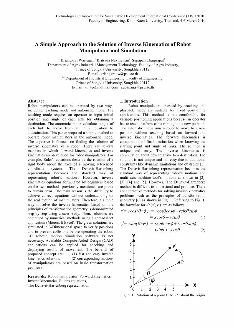
1. Introduction Robot manipulators operated by teaching and playback mode are suitable for fixed positioning applications. This method is not comfortable for variable positioning applications because an operator has to teach that how can a robot go to a new position. The automatic mode runs a robot to move to a new position without teaching based on forward and inverse kinematics. The forward kinematics is computation of final destination when knowing the starting point and angle of links. The solution is unique and easy. The inverse kinematics is computation about how to arrive to a destination. The solution is not unique and not easy due to additional constraints like dynamic limitations and obstacles [1]. The Denavit-Hartenberg representation becomes the standard way of representing robot’s motions and multi-axis machine tool’s motions as shown in [2], [3], [4] and [5]. However, The Denavit-Hartenberg method is difficult to understand and produce. There are alternative methods for solving inverse kinematics problems such as the principles of transformation geometry [6] as shown in Fig. 1. Referring to Fig. 1, the formulae for ( , )P x y′ ′ ′ are as follows: x = rcos( + ) θ φ′ = rcos cos rsin sinθ φ θ φ−

= xcos ysinθ θ− (1) y = rsin( + ) θ φ′ = rsin cos rcos sinθ φ θ φ+

= xsin ycosθ θ+ (2)

Figure 1. Rotation of a point P to P′ about the origin

K. Waiyagan et al. / TISD2010, Thailand, 4-6 March 2010 2

The paper is structured as follows. Section 2 explains the inverse kinematics of a pick and place robot. Section 3 shows simulations of case study. Finally, conclusions are given. 2. The inverse kinematics of a pick and place robot A pick and place robot named Gryphon is used to demonstrate a simple approach to the solution of inverse kinematics by the principles of transformation geometry. The configurations of the robot are shown in Fig. 2 and 3.

Figure 2. Gryphon robot

Figure 3. The configurations of Gryphon robot at the home position

This robot includes 4 axes: Waist 1( )θ , Elbow 2( )θ ,

Shoulder 3( )θ and Wrist/Gripper 4( )θ .The procedures to find the inverse kinematics of the robot are as follow: 1. Assume that a small cylindrical object is located in

any position ( , , )x y z in the workspace of robot.

2. Rotate waist 1( )θ about z-axis so that the diameter of gripper coincides with the diameter of object as shown in Fig. 4. 1θ is computed by Trigonometric functions following equations.

2 2r x y= + (3)

offsetCompensatingAngle( CA ) Arc sine( )r

= (4)

1xArc sin e( )r

θ = CA± (5)

Where:

1xmoves in positve direction Arc sine( ) CAr

θ = −

1xmoves in negative direction Arc sin e( ) CAr

θ = +

3. Calculate 2θ , 3θ and 4θ subjected to the following constraints for rotating elbow, shoulder and wrist about x-axis respectively. 3.1 The tip of gripper touches the object. 3.2 the wrist/gripper is perpendicular to the ground. 3.3 No collisions between components.

2θ , 3θ and 4θ have to satisfy equations (6) & (7)

Where: xY∆ and xZ∆ are the differential displacements by rotating about x coordinate system.

2 3 4r Y Y Yθ θ θ= ∆ + ∆ +∆ (6)

2 3 4z Z Z Zθ θ θ= ∆ +∆ + ∆ (7) Gripper is perpendicular to the ground, so

2 30r Y Yθ θ= ∆ +∆ + (8)

2 3z Z Z lengthof gripperθ θ= ∆ + ∆ − (9)

2Yθ∆ and

2Zθ∆ are calculated by the principles of

transformations as the equation (1) and (2). (Rotation about x-axis at 2θ coordinate system)

2 2 2Y y cos( ) z sin( )θ θ θ∆ = − (10)

2 2 2Z y sin( ) z cos( )θ θ θ∆ = + (11)

(Translation 2θ to 3θ coordinate system)

2 3 2TY Y lengthof shoulderθ θ θ∆ = ∆ + (12)

2 3 20TZ Zθ θ θ∆ = ∆ + (13)

K. Waiyagan et al. / TISD2010, Thailand, 4-6 March 2010 3

(Rotation about x-axis at 3θ coordinate system)

3 2 3 2 33 3T TY Y cos( ) Z sin( )θ θ θ θ θθ θ∆ = ∆ −∆ (14)

3 2 3 2 33 3T TZ Y sin( ) Z cos( )θ θ θ θ θθ θ∆ = ∆ +∆ (15) (Translation 3θ to 1θ coordinate system)

3 1 3TY Y off centerθ θ θ∆ = ∆ + (16)

3 1 30TZ Zθ θ θ∆ = ∆ + (17)

Finally,

3 1Tr Yθ θ= ∆ (18)

3 1Tz Z lengthof gripperθ θ= ∆ − (19) The equations (18) and (19) contain two unknown variables including 2θ and 3θ . Then, solutions are computed by numerical methods using a spreadsheet application (The Solver in Microsoft Excel). 4θ has to be perpendicular to the ground for pick and place operations. Thus,

2 3 4 90θ θ θ+ + = − (20)

Figure 4.Coinciding between two diameters of objects 3. Simulations of Case Study

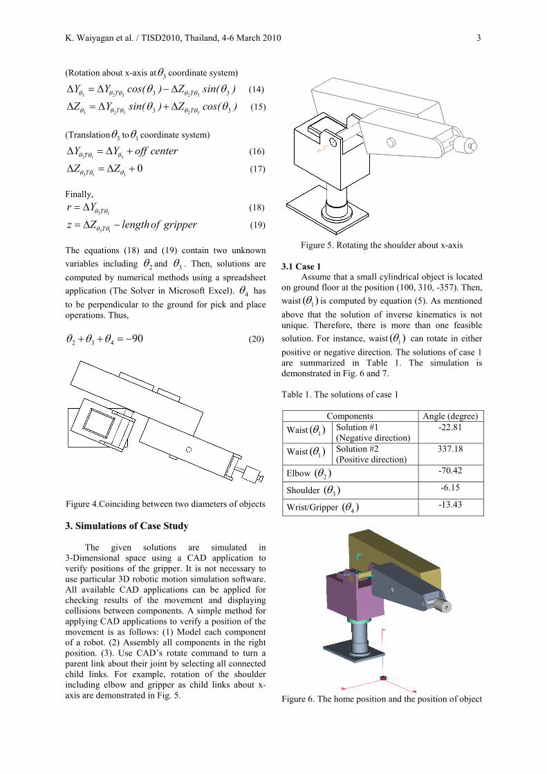
The given solutions are simulated in 3-Dimensional space using a CAD application to verify positions of the gripper. It is not necessary to use particular 3D robotic motion simulation software. All available CAD applications can be applied for checking results of the movement and displaying collisions between components. A simple method for applying CAD applications to verify a position of the movement is as follows: (1) Model each component of a robot. (2) Assembly all components in the right position. (3). Use CAD’s rotate command to turn a parent link about their joint by selecting all connected child links. For example, rotation of the shoulder including elbow and gripper as child links about x-axis are demonstrated in Fig. 5.

Figure 5. Rotating the shoulder about x-axis 3.1 Case 1

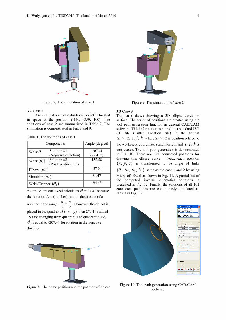
Assume that a small cylindrical object is located on ground floor at the position (100, 310, -357). Then, waist 1( )θ is computed by equation (5). As mentioned above that the solution of inverse kinematics is not unique. Therefore, there is more than one feasible solution. For instance, waist 1( )θ can rotate in either positive or negative direction. The solutions of case 1 are summarized in Table 1. The simulation is demonstrated in Fig. 6 and 7. Table 1. The solutions of case 1

Components Angle (degree) Waist 1( )θ Solution #1

(Negative direction) -22.81

Waist 1( )θ Solution #2 (Positive direction)

337.18

Elbow 2( )θ -70.42

Shoulder 3( )θ -6.15

Wrist/Gripper 4( )θ -13.43

Figure 6. The home position and the position of object

K. Waiyagan et al. / TISD2010, Thailand, 4-6 March 2010 4

Figure 7. The simulation of case 1

3.2 Case 2 Assume that a small cylindrical object is located

in space at the position (-150, -350, 100). The solutions of case 2 are summarized in Table 2. The simulation is demonstrated in Fig. 8 and 9. Table 1. The solutions of case 1

Components Angle (degree)

Waist 1θ Solution #1 (Negative direction)

-207.41 (27.41*)

Waist 1( )θ Solution #2 (Positive direction)

152.58

Elbow 2( )θ -57.04

Shoulder 3( )θ 61.47

Wrist/Gripper 4( )θ -94.43

*Note: Microsoft Excel calculates 1θ = 27.41 because the function Asin(number) returns the arcsine of a

number in the range2π

− to2π . However, the object is

placed in the quadrant 3 ( , )x y− − then 27.41 is added 180 for changing from quadrant 1 to quadrant 3. So,

1θ is equal to -207.41 for rotation in the negative direction.

Figure 8. The home position and the position of object

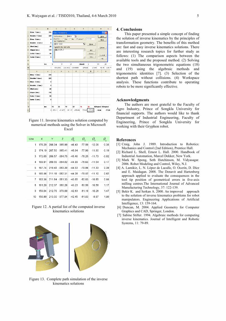
Figure 9. The simulation of case 2 3.3 Case 3 This case shows drawing a 3D ellipse curve on surface. The series of positions are created using the tool path generation function in general CAD/CAM software. This information is stored in a standard ISO CL file (Cutter Location file) in the format

, , , , ,x y z i j k where , ,x y z is position related to the workpiece coordinate system origin and , ,i j k is unit vector. The tool path generation is demonstrated in Fig. 10. There are 101 connected positions for drawing this ellipse curve. Next, each position ( , , )x y z is transformed to be angle of links

1 2 3 4( , , , )θ θ θ θ same as the case 1 and 2 by using Microsoft Excel as shown in Fig. 11. A partial list of the computed inverse kinematics solutions is presented in Fig. 12. Finally, the solutions of all 101 connected positions are continuously simulated as shown in Fig. 13.

Figure 10. Tool path generation using CAD/CAM software

K. Waiyagan et al. / TISD2010, Thailand, 4-6 March 2010 5

Figure 11. Inverse kinematics solution computed by numerical methods using the Solver in Microsoft

Excel

Figure 12. A partial list of the computed inverse kinematics solutions

Figure 13. Complete path simulation of the inverse kinematics solutions

4. Conclusions This paper presented a simple concept of finding the solution of inverse kinematics by the principles of transformation geometry. The benefits of this method are: fast and easy inverse kinematics solutions. There are interesting research topics for further study as follows: (1) The comparison aspects between the available tools and the proposed method. (2) Solving the two simultaneous trigonometric equations (18) and (19) using the algebraic methods and trigonometric identities [7]. (3) Selection of the shortest path without collisions. (4) Workspace analysis. These functions contribute to operating robots to be more significantly effective.

Acknowledgments The authors are most grateful to the Faculty of Agro Industry, Prince of Songkla University for financial supports. The authors would like to thank Department of Industrial Engineering, Faculty of Engineering, Prince of Songkla University for working with their Gryphon robot.

References [1] Craig, John J. 1989. Introduction to Robotics:

Mechanics and Control (2nd Edition), Prentice Hall. [2] Richard L. Shell, Ernest L. Hall. 2000. Handbook of

Industrial Automation, Marcel Dekker, New York. [3] Mark W. Spong, Seth Hutchinson, M. Vidyasagar.

2006. Robot Modeling and Control, Wiley, N.J. [4] A. Lamikiz, L. N. López de Lacalle, O. Ocerin, D. Díez

and E. Maidagan. 2008. The Denavit and Hartenberg approach applied to evaluate the consequences in the tool tip position of geometrical errors in five-axis milling centres.The International Journal of Advanced Manufacturing Technology, 37: 122-139.

[5] Bekir K. and Serkan A. 2000. An improved approach to the solution of inverse kinematics problems for robot manipulators. Engineering Applications of Artificial Intelligence, 13: 159-164.

[6] Duncan, M. 2004. Applied Geometry for Computer Graphics and CAD, Springer, London.

[7] Sabine Stifter. 1994. Algebraic methods for computing inverse kinematics. Journal of Intelligent and Robotic Systems, 11: 79-89.