1

A short course on Altimetry

Paolo Cipollini1, Helen Snaith2 1 National Oceanography Centre, Southampton, U.K.

2 British Oceanographic Data Centre, Southampton, U.K.

with contributions by Peter Challenor, Ian Robinson, R. Keith Raney + some other friends…

2

Outline

• Rationale • why we need altimetry

• A1 – Principles of altimetry • how it works in principle

• New techniques

• A2 – Altimeter Data Processing • From satellite height to surface height: corrections

• (or how it is made accurate)

• A3 – Altimetry and Oceanography

• A4 – Geophysical parameters and applications • what quantities we measure

• how we use them!

3

Rationale for Radar Altimetry over the oceans

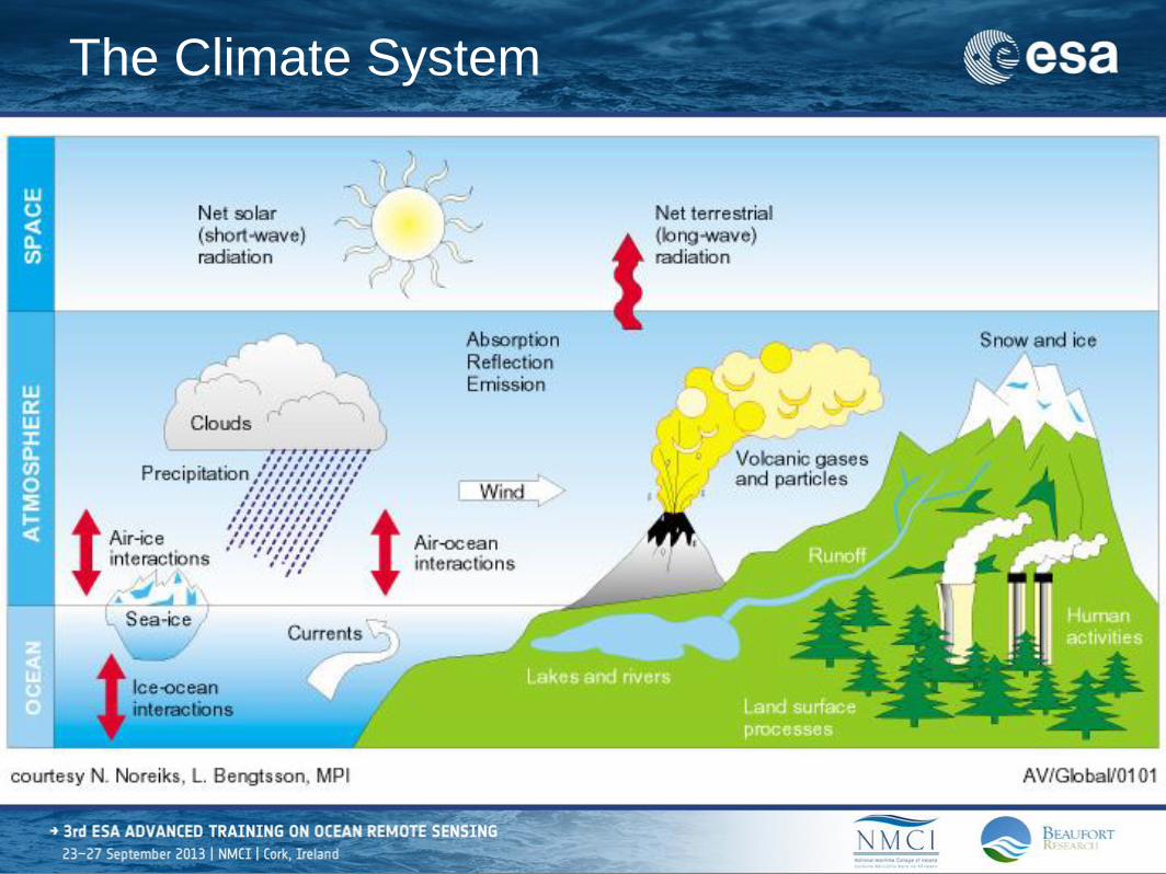
• Climate change • oceans are a very important

component of the climate system

• Altimeters monitor currents / ocean circulation…

• …that can be used to estimate heat storage and transport

• … and to assess the interaction between ocean and atmosphere

• We also get interesting by-products: wind/waves, rain

4

The Climate System

5

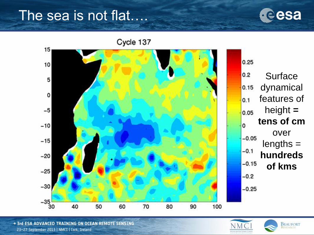
The sea is not flat….

Surface

dynamical

features of

height =

tens of cm

over

lengths =

hundreds

of kms

6

Altimetry 1 –

principles & instruments

P. Cipollini, H. Snaith – A short course on Altimetry

7

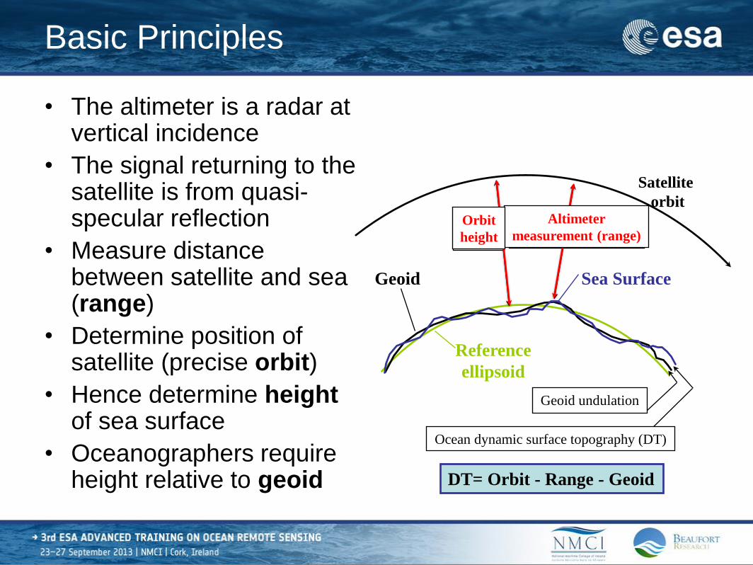
Basic Principles

• The altimeter is a radar at vertical incidence

• The signal returning to the satellite is from quasi-specular reflection

• Measure distance between satellite and sea (range)

• Determine position of satellite (precise orbit)

• Hence determine height of sea surface

• Oceanographers require height relative to geoid

Sea Surface Geoid

Reference

ellipsoid

Satellite

orbit

Orbit

height

Altimeter

measurement (range)

Geoid undulation

Ocean dynamic surface topography (DT)

DT= Orbit - Range - Geoid

Altimeter

measurement (range) Orbit

height

8

Measuring ocean topography with radar

• Measure travel time, 2T,

from emit to return

• h = T×c (c ≈ 3x108 m/s)

• Resolution to ~1cm

would need a pulse of

3x10-10s

(0.3 nanoseconds)

• 0.3ns… That would be a pulse

bandwidth of >3 GHz…

Impossible!

Nadir view

Quasi-Specular reflection

h

(range)

orbit

sea surface

9

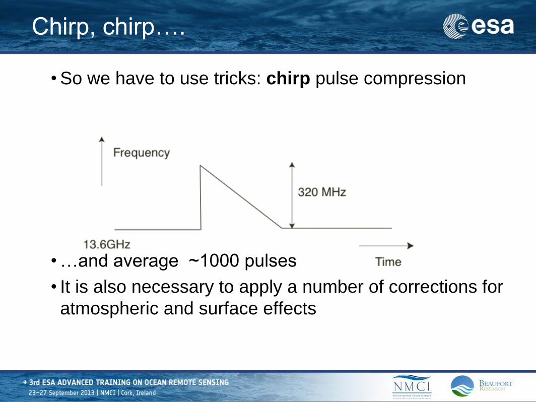
Chirp, chirp….

• So we have to use tricks: chirp pulse compression

• …and average ~1000 pulses

• It is also necessary to apply a number of corrections for

atmospheric and surface effects

10

Beam- and Pulse- Limited Altimeters

• In principle here are two types of altimeter:

• beam-limited

• pulse-limited

11

Beam-Limited Altimeter

• Return pulse is dictated

by the width of the beam

12

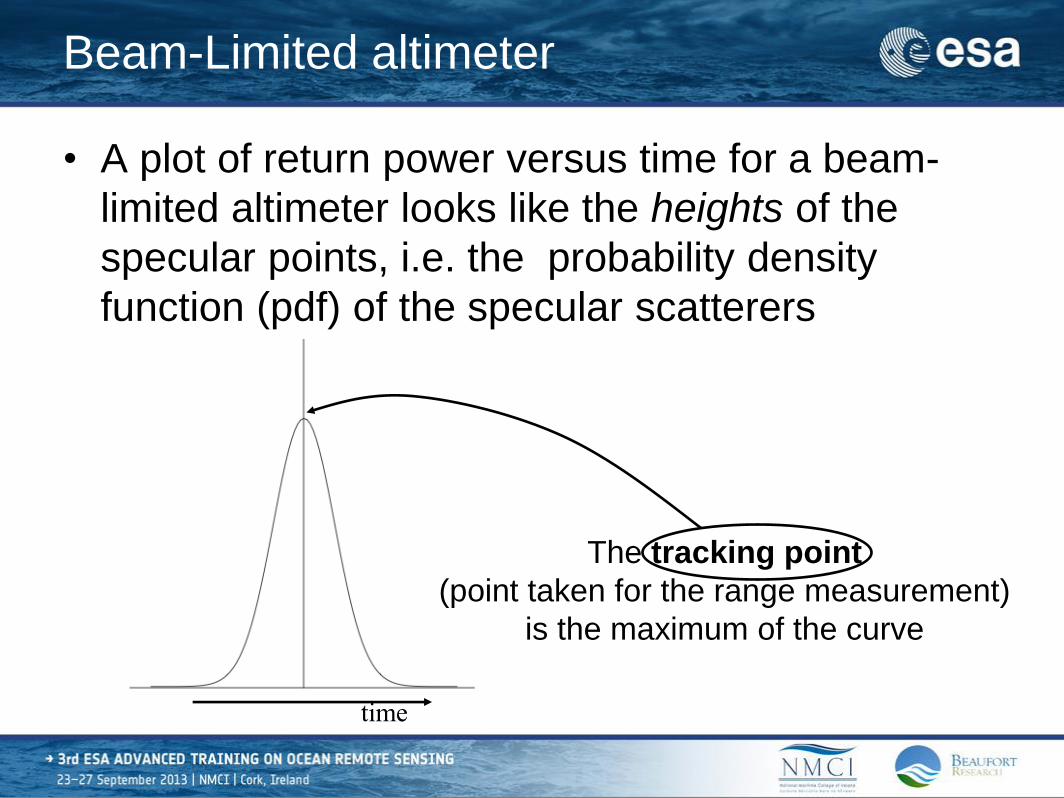
Beam-Limited altimeter

• A plot of return power versus time for a beam-

limited altimeter looks like the heights of the

specular points, i.e. the probability density

function (pdf) of the specular scatterers

The tracking point

(point taken for the range measurement)

is the maximum of the curve

time

13

Beam-Limited: technological problems

• Narrow beams require very large antennae and are impractical in space

• For a 5 km footprint a beam width of about 0.3° is required.

• For a 13.6 GHz altimeter this would imply a 5 m antenna.

• Even more important: highly sensitivity to mispointing, which affects both amplitude and measured range

• New missions like ESA’s CryoSat (launched 8 Apr 2010) and Sentinel-3 use synthetic aperture techniques (delay-Doppler Altimeter) that “can be seen as” a beam-limited instrument in the along-track direction.

14

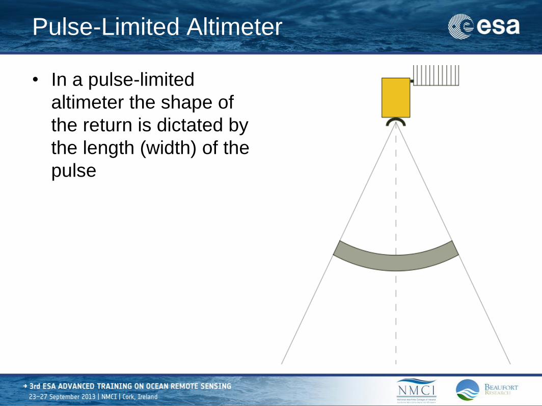
Pulse-Limited Altimeter

• In a pulse-limited

altimeter the shape of

the return is dictated by

the length (width) of the

pulse

15

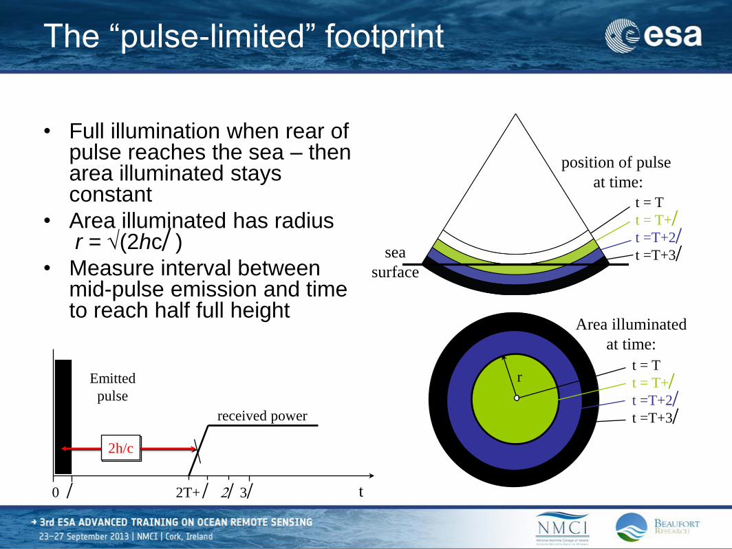
The “pulse-limited” footprint

• Full illumination when rear of pulse reaches the sea – then area illuminated stays constant

• Area illuminated has radius r = (2hc)

• Measure interval between mid-pulse emission and time to reach half full height

position of pulse

at time:

t = T

t = T+

t =T+2

t =T+3 sea

surface

received power

Emitted

pulse

2T+ 3 t 0

2h/c

r

Area illuminated

at time:

t = T

t = T+

t =T+2

t =T+3

2h/c

16

• A plot of return power versus time for a pulse-

limited altimeter looks like the integral of the

heights of the specular points, i.e. the

cumulative distribution function (cdf) of the

specular scatterers

The tracking point is the half

power point of the curve

time

17

Pulse- vs Beam-Limited

• All the microwave altimeters flown in space to

date, including very successful

TOPEX/Poseidon, ERS-1 & 2 RA & Envisat RA-

2, are pulse-limited except….

• … laser altimeters (like GLAS on ICESAT) are

beam-limited

• …and a Delay-Doppler Altimeter “can be seen”

as beam-limited in the along-track direction

• To understand the basics of altimetry we will

focus on the pulse limited design

18

Basics of pulse-limited altimeter theory

• We send out a thin shell of radar energy which is

reflected back from the sea surface

• The power in the returned signal is detected by a

number of gates (bins) each at a slightly different

time

19

Shell of energy from the pulse

20

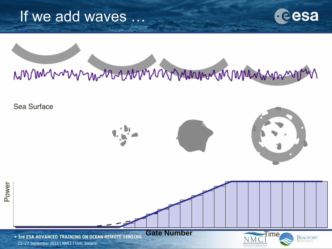
Gate Number

If we add waves …

21

The area illuminated or ‘effective footprint’

• The total area illuminated is related to the

significant wave height noted as SWH [or Hs]

(SWH ≈ 4 × std of the height distribution)

• The formula is

Where c is the speed of light is the pulse length H

s significant wave height

R0 the altitude of the satellite

RE the radius of the Earth

pR0 ct + 2Hs( )1+R0 RE

22

From Chelton et al (1989)

Diameters of the effective footprint

Hs (m) ERS-2/1, ENVISAT

Effective footprint (km)

(800 km altitude)

TOPEX, Jason-1/2

Effective footprint (km)

(1335 km altitude)

0 1.6 2.0

1 2.9 3.6

3 4.4 5.5

5 5.6 6.9

10 7.7 9.6

15 9.4 11.7

20 10.8 13.4

23

The Brown Model

• Assume that the sea surface is a perfectly

conducting rough mirror which reflects only at

specular points, i.e. those points where the radar

beam is reflected directly back to the satellite

24

The Brown Model - II

• Under these assumptions the return power is

given by a three fold convolution

Where

Pr(t) is the returned power

PFS(t) is the flat surface response

PPT(t) is the point target response

PH(-z) is the pdf of specular points on the sea surface

Pr (t) = PFS t( )*PPT t( )*PH -z( )

25

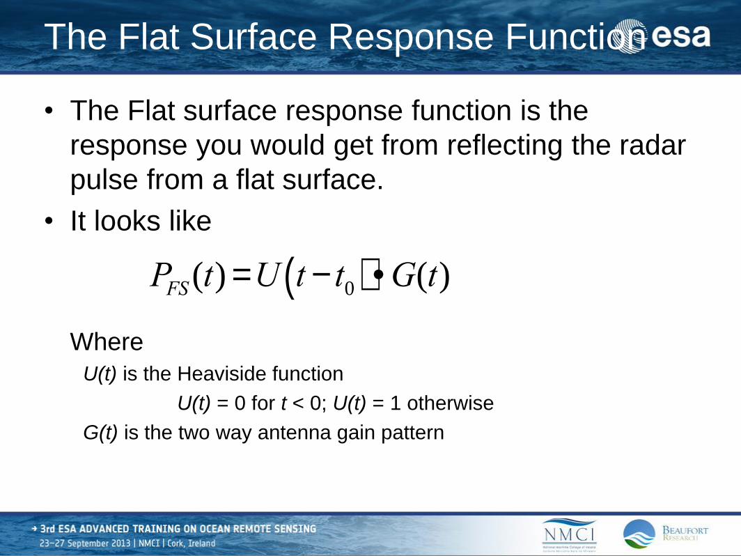
The Flat Surface Response Function

• The Flat surface response function is the

response you would get from reflecting the radar

pulse from a flat surface.

• It looks like

Where

U(t) is the Heaviside function

U(t) = 0 for t < 0; U(t) = 1 otherwise

G(t) is the two way antenna gain pattern

PFS (t) =U t - t0( )·G(t)

26

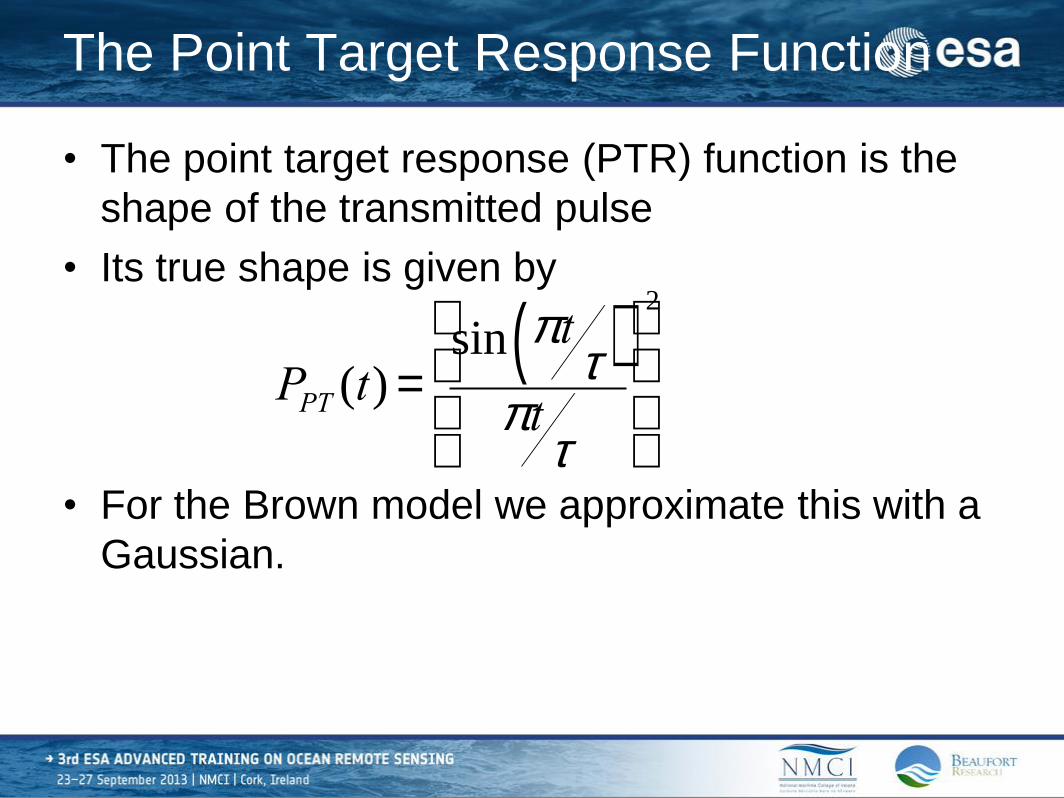
The Point Target Response Function

• The point target response (PTR) function is the

shape of the transmitted pulse

• Its true shape is given by

• For the Brown model we approximate this with a

Gaussian.

PPT (t) =sin p t

t( )p t

t

é

ë

êê

ù

û

úú

2

27

Pr (t) = PFS t - t0( )hPT 2ps p

21+ erf

(t - t0 )

2s c

ìíî

üýþ

é

ëêê

ù

ûúú for t ³ t0

The Brown Model - III

Pr (t) = PFS 0( )hPT 2ps p

21+erf

(t - t0 )

2s c

ìíî

üýþ

é

ëêê

ù

ûúú for t < t0

s c = s p

2 +4s s

2

c2s s »

SWH

4

PFS (t) =G0

2lR2cs 0

4 4p( )2Lph

3exp -

4

gsin2 x -

4ct

ghcos2x

ìíî

üýþI0

4

g

ct

hsin2x

æ

èç

ö

ø÷

28

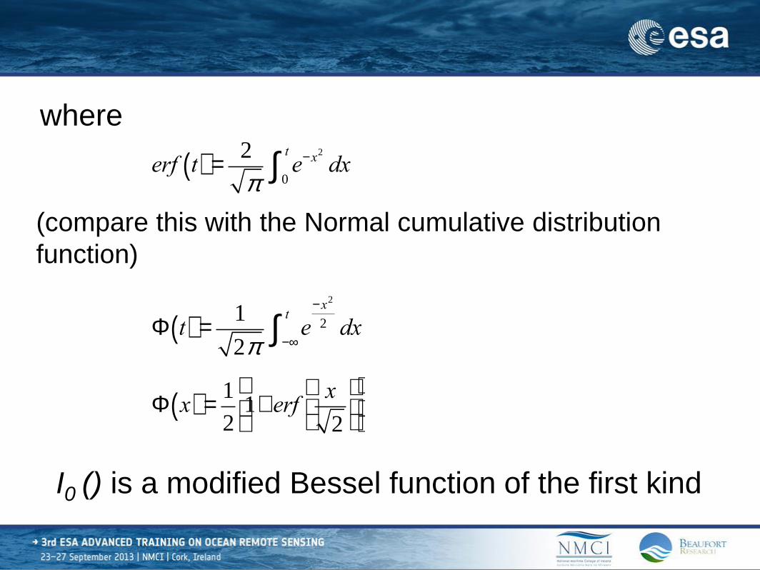
where

(compare this with the Normal cumulative distribution

function)

I0 () is a modified Bessel function of the first kind

erf t( ) =2

pe-x

2

dx0

t

ò

F t( ) =1

2pe

-x2

2 dx-¥

t

ò

F x( ) =1

21+ erf

x

2

æ

èç

ö

ø÷

é

ëê

ù

ûú

29

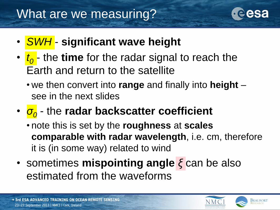
What are we measuring?

• SWH - significant wave height

• t0 - the time for the radar signal to reach the

Earth and return to the satellite

• we then convert into range and finally into height –

see in the next slides

• σ0 - the radar backscatter coefficient

• note this is set by the roughness at scales

comparable with radar wavelength, i.e. cm, therefore

it is (in some way) related to wind

• sometimes mispointing angle ξ can be also

estimated from the waveforms

30

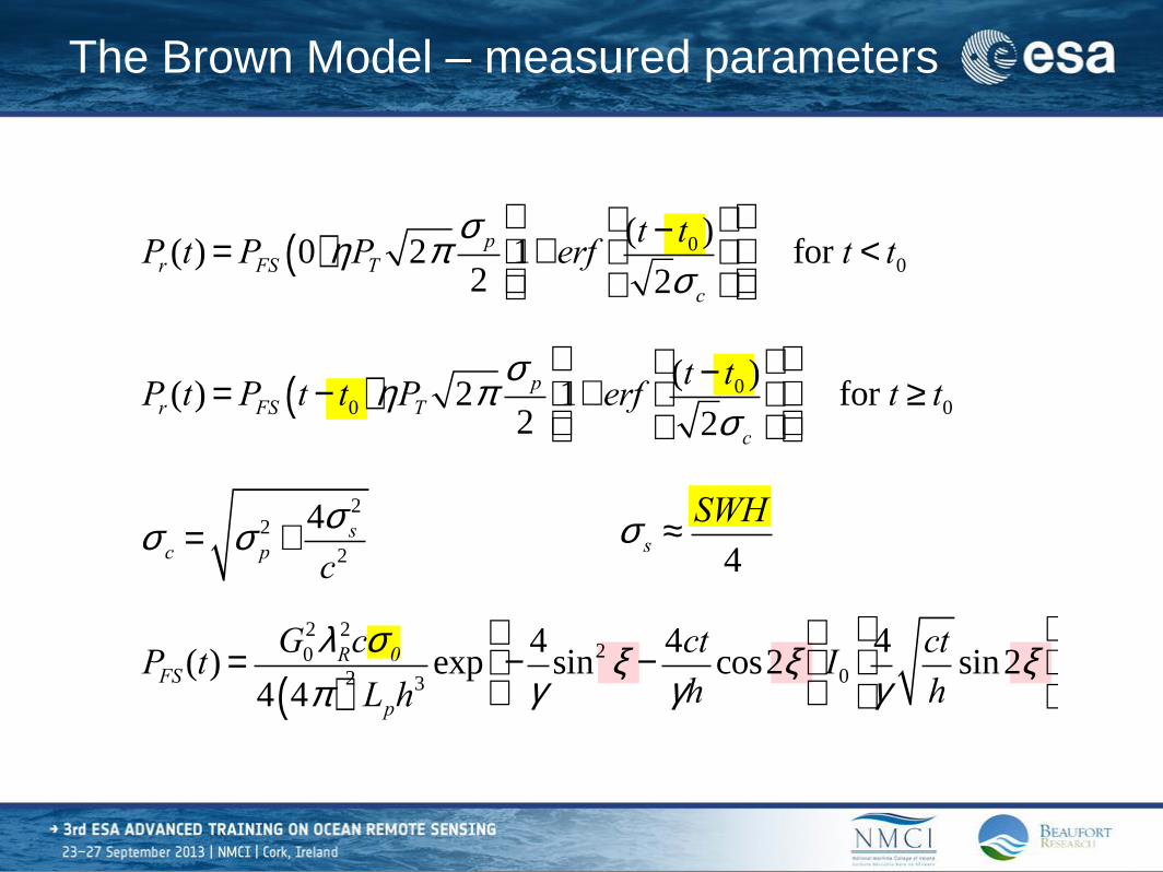
Pr (t) = PFS t - t0( )hPT 2ps p

21+ erf

(t - t0 )

2s c

ìíî

üýþ

é

ëêê

ù

ûúú for t ³ t0

The Brown Model – measured parameters

Pr (t) = PFS 0( )hPT 2ps p

21+erf

(t - t0 )

2s c

ìíî

üýþ

é

ëêê

ù

ûúú for t < t0

s c = s p

2 +4s s

2

c2s s »

SWH

4

PFS (t) =G0

2lR2cs 0

4 4p( )2Lph

3exp -

4

gsin2 x -

4ct

ghcos2x

ìíî

üýþI0

4

g

ct

hsin2x

æ

èç

ö

ø÷

31

What are the other parameters?

• λR is the radar wavelength

• Lp is the two way propagation loss

• h is the satellite altitude (nominal)

• G0 is the antenna gain

• γ is the antenna beam width

• σp is the pulse width

• η is the pulse compression ratio

• PT is the peak power

• ξ (as we said) is the mispointing angle

32

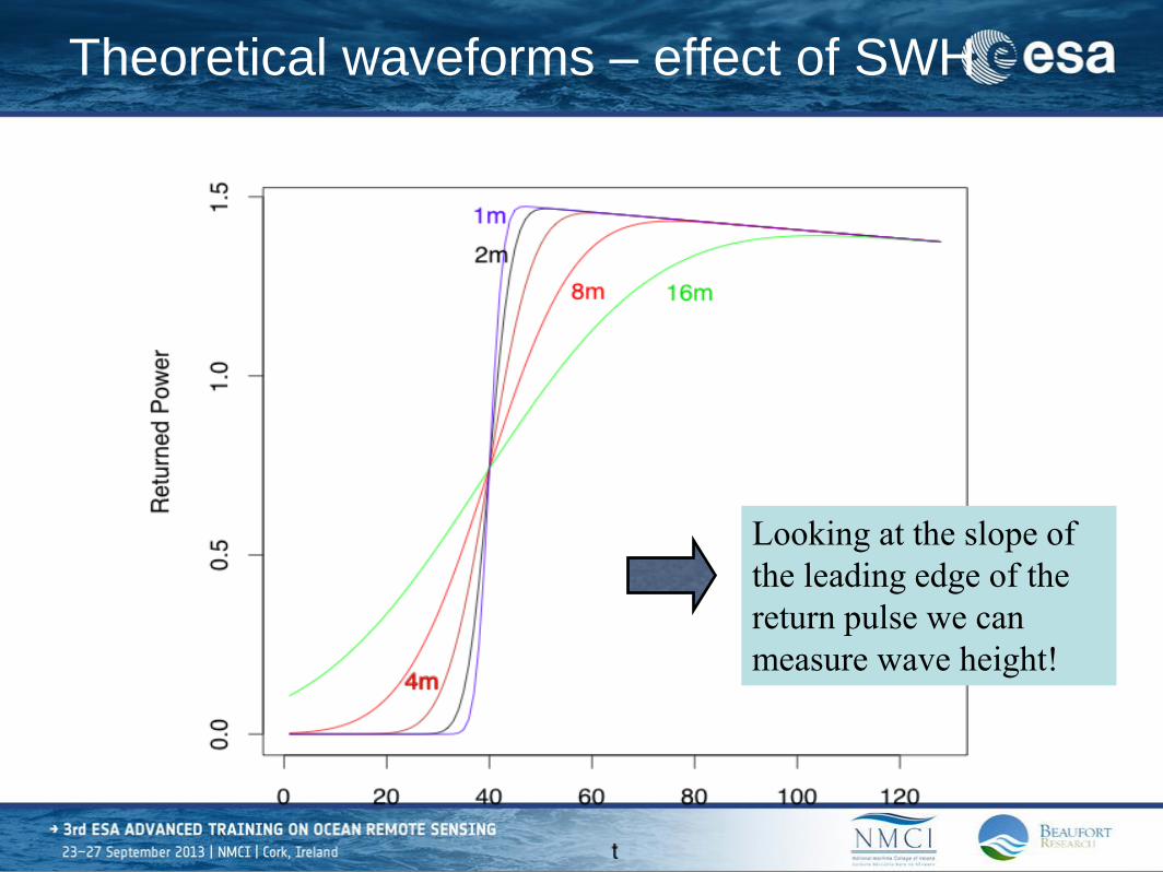
Theoretical waveforms – effect of SWH

Looking at the slope of

the leading edge of the

return pulse we can

measure wave height!

33

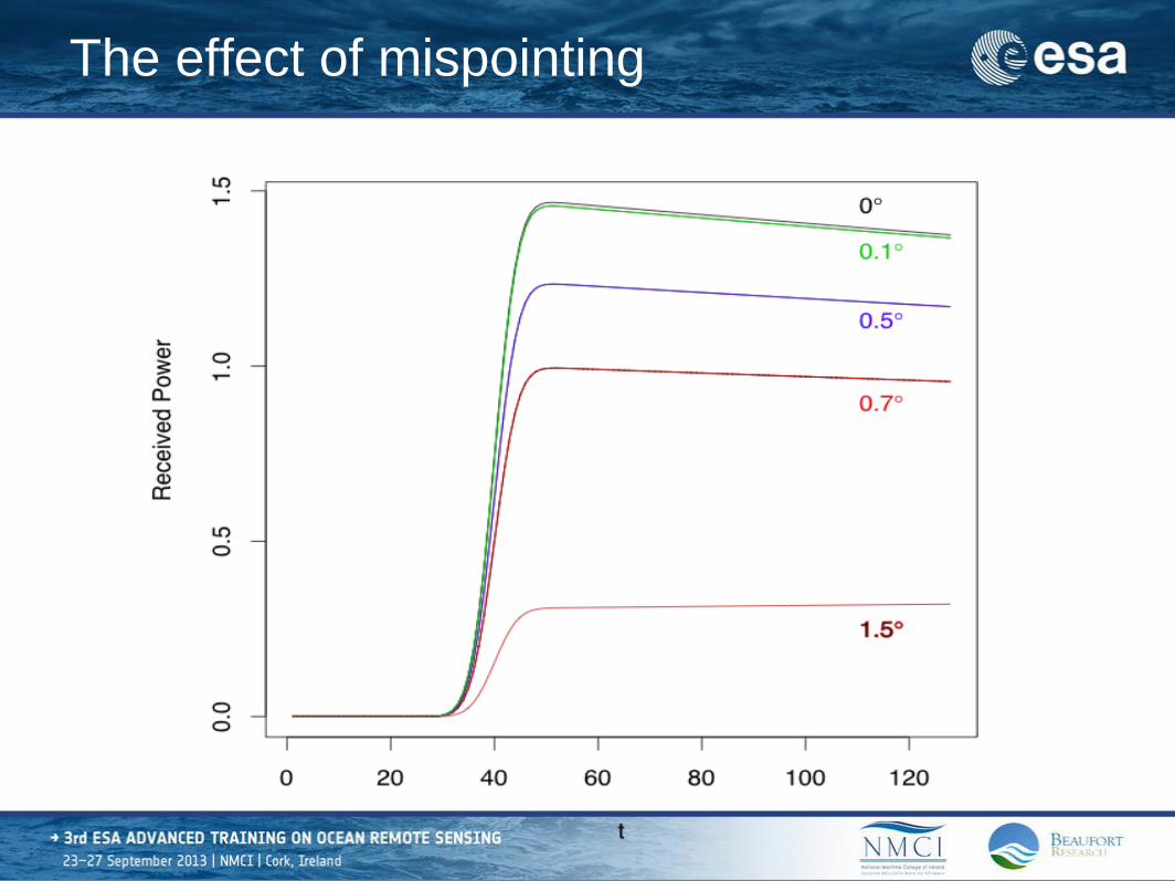
The effect of mispointing

34

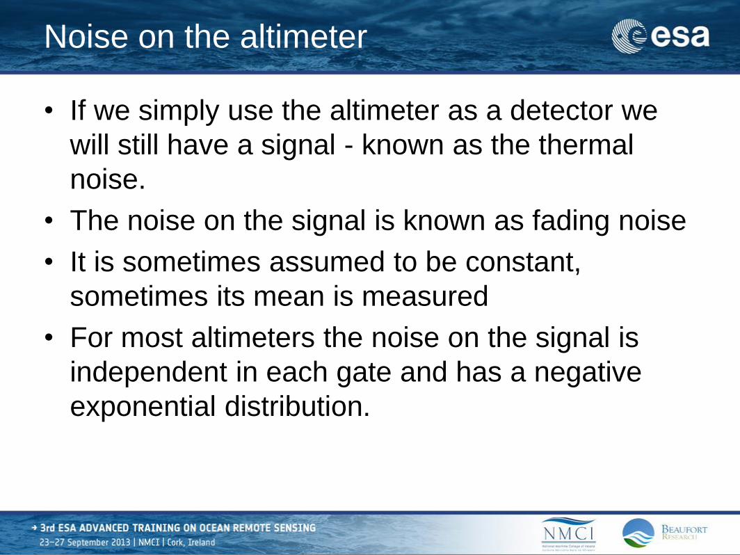
Noise on the altimeter

• If we simply use the altimeter as a detector we

will still have a signal - known as the thermal

noise.

• The noise on the signal is known as fading noise

• It is sometimes assumed to be constant,

sometimes its mean is measured

• For most altimeters the noise on the signal is

independent in each gate and has a negative

exponential distribution.

35

Exponential distribution

• pdf

• Mean = θ

• Variance = θ2

 

f (x) =1

qe

-x

q0 < x < ∞

36

Exponential pdf

37

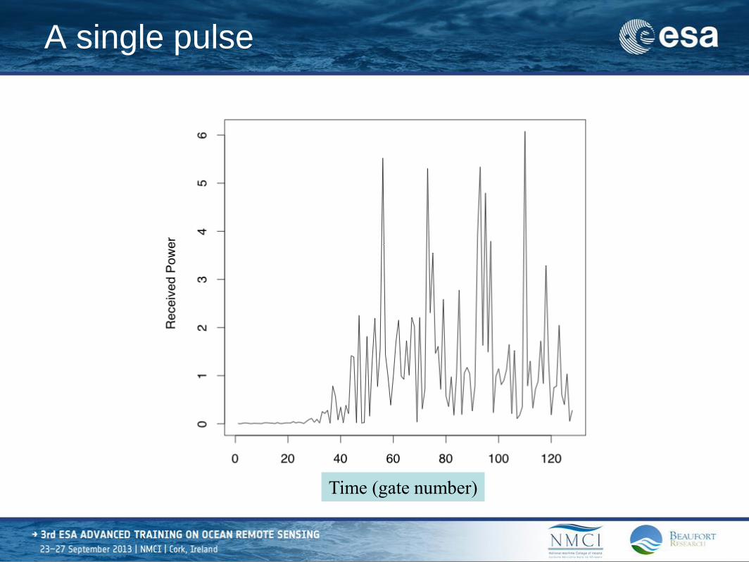
Averaging the noise

• For a negative exponential distribution the

variance is equal to the square of the mean.

Thus the individual pulses are very noisy!

➱ We need a lot of averaging to achieve good

Signal to Noise Ratio

• The pulse repetition frequency is thousands per

second

• 1020 for ERS-1/2, 1800 for Jason & Envisat, 4500 for

Topex

• Usually data are transmitted to the ground at

~20Hz and then averaged to ~1 Hz

38

A single pulse

Time (gate number)

39

Time (gate number)

40

• It is very difficult (if not impossible) to generate a single-frequency pulse of length 3 ns

• It is possible to do something very similar in the frequency domain using a chirp: modulating the frequency of the carrier wave in a linear way

• The equivalent pulse width = 1/chirp bandwidth

How altimeters really work

41

Transmit Receive

Delay

Generate

chirp Combine

Full chirp deramp - 1

• A chirp is generated

• Two copies are taken

• The first is transmitted

• The second is delayed

so it can be matched

with the reflected pulse

42

Full Chirp Deramp - 2

• The two chirps are mixed.

• A point above the sea surface gives returns at

frequency lower than would be expected and

vice versa

• So a ‘Brown’ return is received but with

frequency rather than time along the x axis

43

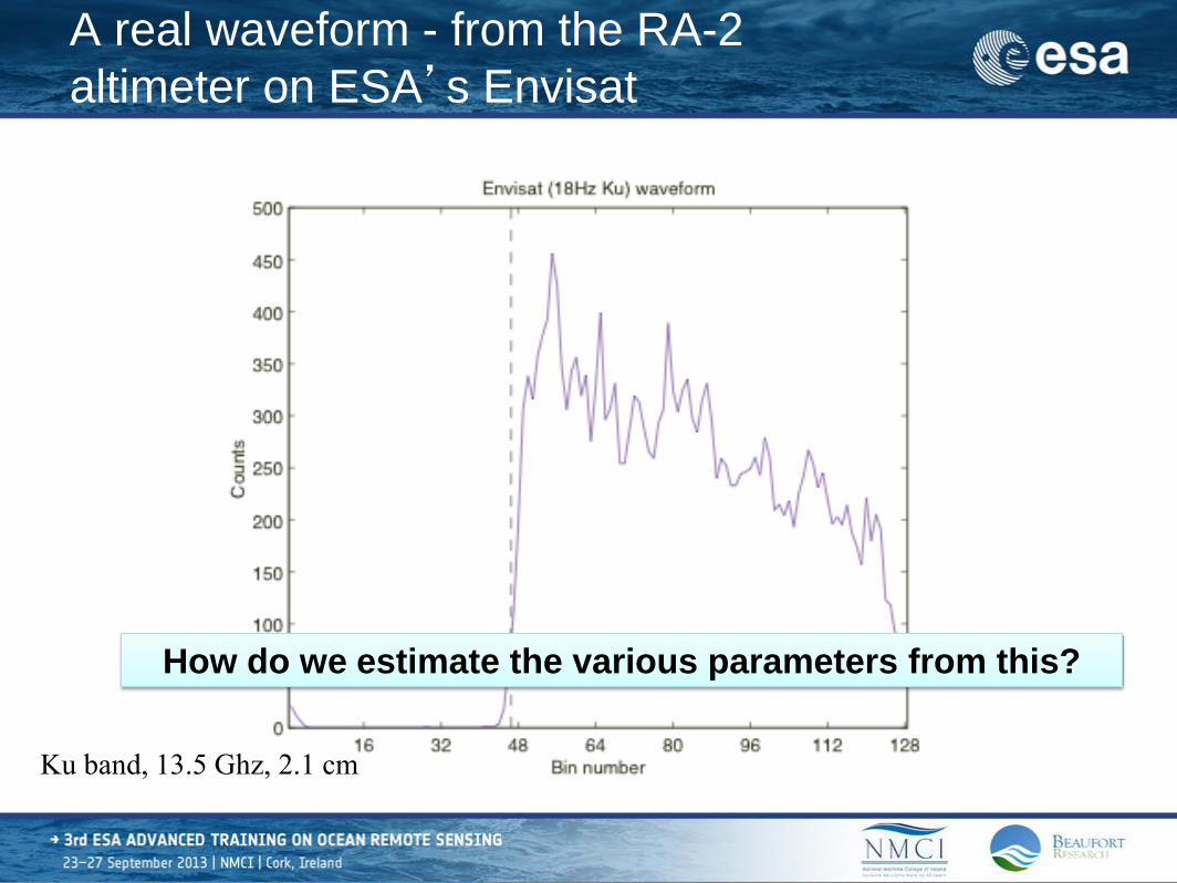
A real waveform - from the RA-2

altimeter on ESA’s Envisat

Ku band, 13.5 Ghz, 2.1 cm

How do we estimate the various parameters from this?

44

“Retracking” of the waveforms

= fitting the waveforms with a waveform model,

therefore estimating the parameters

Figure from J Gomez-Enri et al. (2009)

Maximum amplitude:

related to wind speed

“Epoch”: gives range

(therefore height)

Slope of leading edge:

related to significant

wave height

45

Altimeters flown in space

Height inclination accuracy repeat period

GEOS-3 (04/75 – 12/78)

845 km 115 deg 0.5 m -

Seasat (06/78 – 09/78)

800 km 108 deg 0.10 m 3 days

Geosat (03/85 – 09/89)

785.5 km 108.1 deg 0.10 m 17.5 days

ERS-1 (07/91 – 03/2000); ERS-2 (04/95 – 09/2011)

785 km 98.5 deg 0.05 m 35 days

TOPEX/Poseidon (09/92 – 10/2005); Jason-1 (12/01 – 06/2013); Jason-2 (06/08 – present)

1336 km 66 deg 0.02 m 9.92 days

Geosat follow-on (GFO) (02/98 – 09/2008)

800 km 108 deg 0.10 m 17.5 days

Envisat (03/02 – 04/12)

785 km 98.5 deg 0.03 m 35 days

CryoSat-2 (04/10 – present) [delay-Doppler]

717 km 92 deg 0.05 m 369 days (30d sub-cycle)

SARAL/AltiKa (02/13 – present) [Ka-band]

785 km 98.5 deg 0.02 m 35 days

46

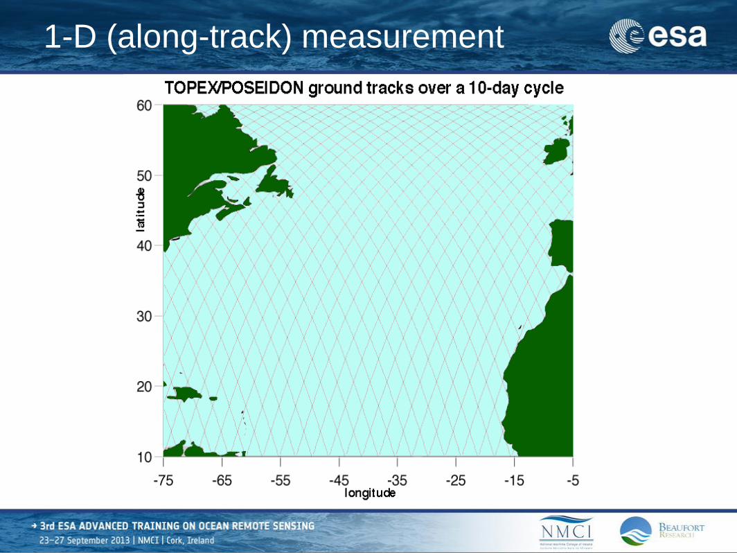
1-D (along-track) measurement

47

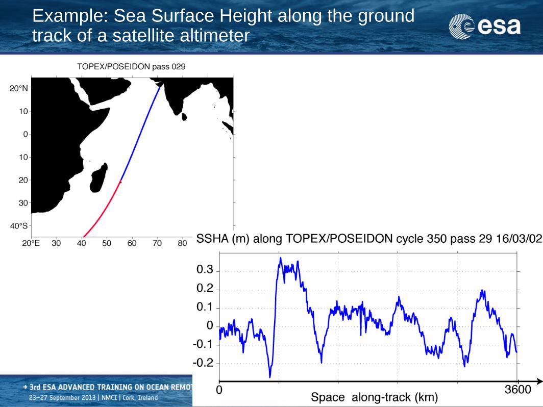
Example: Sea Surface Height along the ground track of a satellite altimeter

48

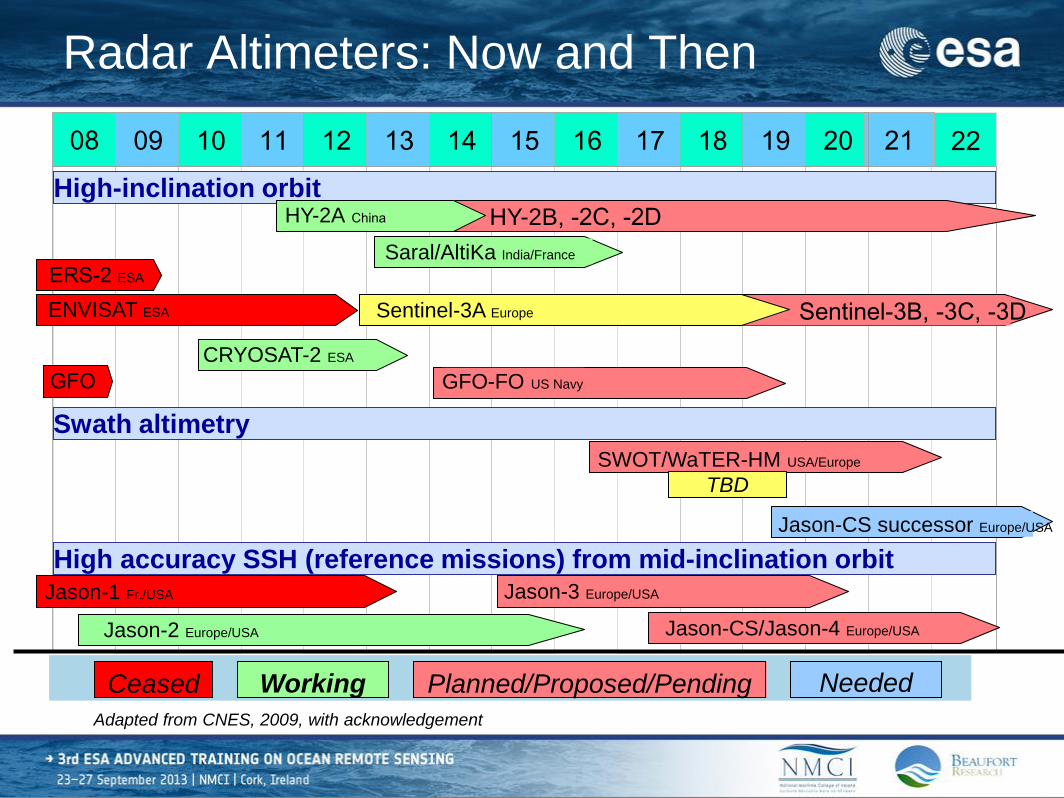
Radar Altimeters: Now and Then

10 11 12 13 14 15 16 17 18 19 20 22 21 09 08

Jason-1 Fr./USA

ENVISAT ESA

High accuracy SSH (reference missions) from mid-inclination orbit

CRYOSAT-2 ESA

High-inclination orbit

Jason-2 Europe/USA

Jason-3 Europe/USA

Jason-CS/Jason-4 Europe/USA

Swath altimetry

SWOT/WaTER-HM USA/Europe

Saral/AltiKa India/France

Jason-CS successor Europe/USA

Ceased Working Planned/Proposed/Pending Needed

TBD

Sentinel-3B, -3C, -3D Sentinel-3A Europe

HY-2B, -2C, -2D HY-2A China

ERS-2 ESA

GFO GFO-FO US Navy

Adapted from CNES, 2009, with acknowledgement

49

Cryosat-2

• ESA mission; launched 8 April 2010

• LEO, non sun-synchronous • 369 days repeat (30d sub-cycle)

• Mean altitude: 717 km

• Inclination: 92°

• Prime payload: SIRAL • SAR/Interferometric Radar

Altimeter (delay/Doppler)

• Modes: Low-Res / SAR / SARIn

• Ku-band only; no radiometer

• Design life: • 6 months commissioning + 3

years

50

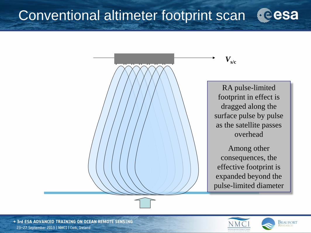
Conventional altimeter footprint scan

Vs/c ) ) ) ) ) )

RA pulse-limited

footprint in effect is

dragged along the

surface pulse by pulse

as the satellite passes

overhead

Among other

consequences, the

effective footprint is

expanded beyond the

pulse-limited diameter

)

51

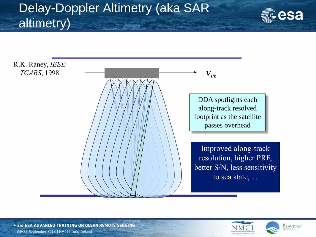
Delay-Doppler Altimetry (aka SAR

altimetry)

Vs/c

DDA spotlights each

along-track resolved

footprint as the satellite

passes overhead

) ) ) ) ) ) ) Improved along-track

resolution, higher PRF,

better S/N, less sensitivity

to sea state,…

R.K. Raney, IEEE

TGARS, 1998

52

DDA (SAR-mode) Footprint

Characteristic

Vs/c ) ) ) ) ) ) ) ) ) ) )

Tracker “reads”

waveforms only

from the center

(1, 2, or 3)

Doppler bins

Result? Rejects

all reflections

from non-nadir

sources

Each surface

location can be

followed as it is

traversed by

Doppler bins

53

SARAL / AltiKa

• Satellite: Indian Space Research Organization (ISRO) • carrying AltiKa altimeter by CNES

• Ka-band 0.84 cm (viz 2.2 cm at Ku-band)

• Bandwidth (480 MHz) => 0.31 ρ (viz 0.47)

• Otherwise “conventional” RA

• PRF ~ 4 kHz (viz 2 kHz at Ku-band)

• Full waveform mode

• payload includes dual-frequency radiometer

• Sun-synchronous, 35-day repeat cycle (same as ERS/Envisat)

• Navigation and control: DEM and DORIS

• Launched February 2013

GNSS (GPS/Galileo) Reflectometry

and sea level (tricky!)