a sequential quadratic hamiltonian method for solving ... · al [email protected]...
TRANSCRIPT
A sequential quadratic Hamiltonian method for solvingparabolic optimal control problems with discontinuous cost
functionals
Tim Breitenbach∗ Alfio Borzı†
Abstract
A sequential quadratic Hamiltonian (SQH) method for solving control-constrained parabo-lic optimal control problems with continuous and discontinuous non-convex cost functionalsis investigated. The solution to these problems is characterised by the Pontryagin’s maxi-mum principle, which is also the starting point for the development of a sequential quadraticHamiltonian scheme. In a general setting that includes discontinuous and non-convex costfunctionals, it is proved that the SQH method is well-defined; however, convergence to anoptimal solution is proved only in the smooth case. Results of numerical experiments arepresented that successfully validate the proposed optimisation framework and demonstrateits effectiveness and large applicability.
This is a preprint of the paper
Tim Breitenbach and Alfio Borzı ,A Sequential Quadratic Hamiltonian Method for Solving Parabolic
Optimal Control Problems with Discontinuous Cost Functionalsappeared in Journal of Dynamical and Control Systemshttps://doi.org/10.1007/s10883-018-9419-6
Keywords – Parabolic optimal control problems, discontinuous cost functionals, Pontryaginmaximum principle, iterative scheme
MSC – 49K20, 49M05, 65K10
1 Introduction
Optimal control of parabolic models with cost functionals for which necessary first-order conditionscan be reformulated as semi-smooth equations is a well developed modern research topic; see, e.g.,[22, 45] and references therein. In this framework, optimal solutions are characterised by first-order
∗Institut fur Mathematik, Universitat Wurzburg, Emil-Fischer-Strasse 30, 97074 Wurzburg, Germany;[email protected]
†Institut fur Mathematik, Universitat Wurzburg, Emil-Fischer-Strasse 30, 97074 Wurzburg, Germany;[email protected]
1
optimality conditions that require semi-smoothness of the reduced cost functional allowing thedevelopment of different solution procedures like proximal methods [39] and semi-smooth Newton-methods [45]. However, in the case of cost functionals that are not Lipschitz continuous and inthe much less investigated case of discontinuous cost functionals, the property of semi-smoothnessis lost and the optimisation techniques mentioned above cannot be used, unless regularisation isconsidered at the cost of modifying the nature of the problem; see, e.g., [32].
We mainly focus on discontinuous and non-convex cost functionals as the most challengingbenchmark that can be addressed by the method proposed in this work. In particular, we considera cost functional given by the following:
∫ T0
∫Ωg (u (x, t)) dxdt where the control’s cost is evaluated
with the lower semi-continuous function
g (z) =
|z| if |z| > s
0 otherwise
where s > 0.Our numerical approach has obviously much larger applicability. Discontinuous cost functionals
and, more generally, discontinuous variational problems appear already in the study of jet flows,cavity problems and in plasma physics [6, 29]. However their numerical realisation has beenhindered by the lack of appropriate solvers. In this framework, the purpose of our work is tocontribute to the field of non-smooth optimisation with partial differential equations (PDEs) bydeveloping numerical tools that apply to non-regularised distributed parabolic optimal controlproblems with discontinuous and non-convex cost functionals. For this purpose, we deal withthe optimal control theory based on the Pontryagin’s maximum principle (PMP) [9, 17, 35] thatwas originally developed for control problems governed by ordinary differential equations (ODEs)and has been much less investigated in the context of time-dependent PDE models; see, e.g.,[14, 30, 36, 42, 43]. In particular, we focus on the work [36] to characterise a solution to ourparabolic control problems with a necessary optimality condition provided by the PMP. For theseproblems we briefly address the issue of existence of optimal controls and then turn our attentionto their PMP characterisation.
Although the PMP principle represents a powerful theoretical tool, its use in the PDE contexthas been hindered by the lack of efficient numerical implementation. In fact, well-known directand indirect methods used to solve ODE control problems are difficult to apply in the higherspace-time dimensional setting of PDE problems and in the case of large-size ODE problems. It isthe main purpose of the present work to address this issue by developing an efficient optimisationscheme that is consistent with the PMP framework. For this purpose, we notice that a naturalapproach to solve PDE models is by iterative methods that exploit the sparsity of discretizedPDEs. Moreover, we point out that the PMP principle has a pointwise formulation and evenits proof is by ‘needle variations’, and both are local in structure. Therefore it seems naturalto consider iterative strategies that implement local updates of the control function pointwise inspace and time.
For this reason, we focus on the iterative scheme first proposed in [38] and further discussed in[10, 40] to solve ODE control problems by an augmented Hamiltonian technique and discuss theirextension to our PDE setting. Moreover, we also would like to mention the earlier works [26, 27]where different so-called successive iteration solvers based on the minimisation of the Pontryagin-Hamilton function are considered. Specifically, in [26] the Hamiltonian without augmentation isused to find an update for the control, but, as the authors mention, the issue of convergence
2

remains open for this approach. In any case, we have implemented the method in [26] and foundthat it has difficulty to cope with our cost functionals. In [27], modifications of the method in[26] are discussed that transform the state equation to obtain a weakly controlled problem or usea damping of the control update. The third proposed alternative is to restrict the change of thecontrol to a short time window. In our opinion, the augmented Hamiltonian approach can be seenhaving the same purpose: keep the updates of the control conveniently small.
We remark that the iterative schemes in [26, 27] are designed so that the values of the statevariable from the previous iteration are used while computing the update of the control in thenew iteration sweep. This important feature is also characteristic of the method that we proposein this paper. Therefore we could say that our approach includes different aspects of the methodsproposed in [38, 40] and in [26, 27].
In our approach, we pointwise minimise an augmented Hamiltonian function to find an updatefor the control that provides a better cost functional value. In doing this, we use the statefunction of the governing model from the previous iteration, thus avoiding to recalculate thisfunction every time after a local control update as in [38, 40]. Our procedure results in a muchsmaller number of solving of the state equation, which is necessary since these calculations arevery costly in the case of partial differential equations. In this way, we formulate a new efficientand robust iterative procedure that is able to solve discontinuous optimisation problems while notrelying on regularisation techniques as in [21, 23, 24]. We would like to name our method thesequential quadratic Hamiltonian (SQH) scheme and show that it is able to solve discontinuoustime-dependent parabolic optimal control problems with almost linear computational complexity.To the best of our knowledge, there is no other available methodology with similar capability. Inthis paper, we theoretically discuss the convergence properties of our iterative SQH method anddemonstrate numerically its effectiveness.
In the next section, we formulate a class of parabolic optimal control problems and discussthe necessary functional estimates. In Section 3, we discuss the Pontryagin maximum principlefor the chosen parabolic optimal control problems. We outline the proof of the PMP principle(Theorem 3.3), which is analogous to [36], providing a necessary optimality condition for ouroptimisation problems with a discontinuous cost of the control. In Section 4, we discuss our PMP-based SQH scheme. We discuss how our scheme provides updates to the control that correspondto monotonically decreasing cost functional values for our optimisation problem. Furthermore, inthe case of a differentiable cost functional, we prove convergence of the SQH sequence to a localoptimal solution in the sense that appropriate first-order optimality conditions are satisfied. Themain results of Section 4 are Theorem 4.1 and Theorem 4.2. In Section 5, results of numericalexperiments considering different cost functionals are presented that successfully demonstrate thealmost optimal complexity of our SQH scheme and its robustness with respect to changes of thevalues of the optimisation parameters. In particular, we show that the solution obtained with theSQH scheme fulfils the PMP optimality condition. Furthermore, to allow a comparison with awell-known optimisation scheme as the non-linear conjugated gradient (NCG) method, we considerthe case of a continuous cost functional and compare our iterative scheme with the NCG method.Notice that a direct comparison of the SQH scheme with the method in [38] results obviously infavour of our method since the latter requires a prohibitive large number of forward solves.
In order to provide all technical details supporting our work and to make this work self-contained as far as possible, we include an appendix. In the Appendix, we prove an L∞-resultfor linear parabolic partial differential equations that is essential for the PMP characterization of
3
parabolic PDE control problems. We include this result since it is usually stated without proofby making references to [28] where the required result is embedded in a more general framework.Further, in the attempt to give a theoretical support to our framework with discontinuous costfunctionals, we prove existence of a minimiser for this optimisation setting in the case of a compactadmissible control set. A section of conclusion completes this work.
2 Formulation of the optimal control problem
In this section, we formulate our parabolic optimal control problems with discontinuous costfunctionals and discuss existence of optimal controls. Our governing model is a heat equationwith distributed control that is defined in the space-time cylinder Q = Ω× (0, T ), Ω ⊂ Rn, n ∈ N,where Ω is an open bounded domain with a smooth boundary. We choose homogeneous Dirichletboundary conditions and an initial condition y0 ∈ L∞ (Ω).
For each t ∈ (0, T ), T > 0, the weak formulation of the resulting initial-boundary valueproblem is as follows: Find y ∈ L2 (0, T ;H1
0 (Ω)) and y′ ∈ L2 (0, T ;H−1 (Ω)), that means, y ∈W (0, T ) := y ∈ L2 (0, T ;H1
0 (Ω)) | y′ ∈ L2 (0, T ;H−1 (Ω)); see [44, Chapter 3], such that thefollowing is satisfied
(y′ (·, t) , v) +D (∇y (·, t) ,∇v) = (u (·, t) , v) in Q
y (·, 0) = y0 on Ω× t = 0 (1)
y = 0 on ∂Ω,
for all v ∈ H10 (Ω). In this setting, y : Q → R denotes the state variable and u : Q → R denotes
the control. We denote with (·, ·) the scalar product in L2 (Ω), D > 0 is the diffusion coefficient,y′ := ∂
∂ty (x, t), and ∇ denotes the L2 (Ω) gradient.
Requiring u ∈ Lq (Q), q > n2
+1 if n ≥ 2 and q ≥ 2 if n = 1, we have that there exists an uniquesolution y ∈ W (0, T ) to (1), see [19, Chapter 7.1, Theorem 3] as y0,∈ L2 (Ω) and u ∈ L2 (Q),see [1, Theorem 2.14]. However, for the aim of the Pontryagin maximum principle, this regularityresult needs to be improved. For this purpose, we require y0 ∈ H1
0 (Ω) ∩ L∞ (Ω). Then we havey ∈ L2 (0, T ;H2 (Ω)) ∩ L∞ (0, T ;H1
0 (Ω)), see [19, Chapter 7 Theorem 5], such that we can applyTheorem 6.1 (Appendix) and have the following theorem.
Theorem 2.1. Let y be the solution to (1). Then, y is essentially bounded by
‖y‖L∞(Q) ≤ ‖y0‖L∞(Ω) + C‖u‖Lq(Q),
where C > 0 is a constant.
Furthermore, we have that the control-to-state map, S : Lq (Q) → W (0, T ), u 7→ y = S (u)is affine and continuous; see [44, (3.36)] and [1, Theorem 2.14] for the continuous embedding ofLq (Q) → L2 (Q). Moreover, the map S is continuous as a map S : Lq (Q) → L2 (Q), since
‖y‖2L2(Q) =
∫ T0‖y‖2
L2(Ω)dt ≤∫ T
0‖y‖2
H10 (Ω)
dt = ‖y‖L2(0,T ;H10 (Ω)).
4

Next, we discuss the following parabolic optimal control problem
miny,u
J (y, u)
s.t. (y′, v) +D (∇y,∇v) = (u, v) in Q
y (·, 0) = y0 on Ω× t = 0 (2)
y = 0 on ∂Ω
u ∈ Uad,
where the cost functional J is given by
J (y, u) := Jc (y, u) + γ
∫Q
g (u (x, t)) dxdt. (3)
In this functional, Jc represents a smooth functional objective as it appears in many controlproblems [11, 44]. We have
Jc (y, u) :=1
2||y − yd||2L2(Q) +
α
2||u||2L2(Q), α ≥ 0. (4)
In this case, the functional Jc models the task of driving the state y to track a desired statetrajectory yd ∈ Lq (Q), while keeping small the L2(Q)-cost of the control.
In addition to Jc, we have a possibly discontinuous cost functional given by
G (u) := γ
∫Q
g (u (x, t)) dxdt, γ ≥ 0, (5)
where g : R→ R is a non-negative and lower semi-continuous function.In particular, we consider the case where
g (u) =
|u| if |u| > s
0 otherwise
where s > 0. With this construction, we obtain a cost of the control that is zero if its value isbelow a given threshold and it measures a L1 cost otherwise. Notice that with this choice thereduced cost functional J (u) := J (S (u) , u) is discontinuous in Lq (Q).
The admissible set of controls is defined as follows
Uad := u ∈ Lq (Q) | u (x, t) ∈ KU, (6)
where KU is a compact subset of R.In the case where G is a convex and continuous cost functional, existence of an optimal control
is guaranteed [44]. However, in the case of discontinuous cost functionals the issue of existence ofan optimal control is more delicate because the property of weakly lower semi-continuous is lost.However, existence of an optimal solution can be proved considering a set of admissible controlsthat is compact in Lq (Q); see Theorem 6.2 in the Appendix. For our purpose, we assume that(2) admits a solution in Uad given in (6).
5

3 The Pontryagin’s maximum principle
In this section, we discuss the characterisation of optimal controls in Uad in the framework ofthe Pontryagin’s maximum principle in its easier variant with no final state constraints; see, e.g.,[30, 36].
First, we illustrate the main theoretical steps in the derivation of the Pontryagin’s maximumprinciple, also with the purpose to introduce essential concepts that are instrumental for thediscussion on our SQH scheme. In the following, the notation var1 ← var2 means that thevariable var1 is set equal to var2.
We formulate the following adjoint problem
(−p′ (·, t) , v) +D (∇p (·, t) ,∇v) = (y (·, t)− yd (·, t) , v) in Q
p (·, T ) = 0 on Ω× T = 0p = 0 on ∂Ω.
(7)
This problem has the same structure as (1) after a transformation of the time variable t := T − τand noticing that y − yd ∈ Lq (Q), see [1, Theorem 2.14]. Hence, there exists an unique p ∈L2 (0, T ;H1
0 (Ω)) and p′ ∈ L2 (0, T ;H−1 (Ω)) solving (7) for all v ∈ H10 (Ω).
Next, we define the Hamiltonian corresponding to (2) - (4) as follows
H (x, t, y, u, p) =1
2(y − yd)2 +
α
2u2 + γg (u) + p u, (8)
where H : Rn × R+0 × R ×KU × R → R. If y, u and p are functions, then H (x, t, y, u, p) stands
short for H (x, t, y(x, t), u(x, t), p(x, t)). We remark that throughout this work, we sometimes dropthe arguments (x, t) of functions to save notational effort when the functional dependence is clearfrom the context.
The classical approach to prove the PMP principle is by the method of needle variation [17, 36].For this purpose, let Sk (x0, t0) be an open ball centered at (x0, t0) ∈ Q with radius skx0,t0 such thatthe Lebesgue measure of the ball tends to zero as k →∞, limk→∞ |Sk (x0, t0) | = 0. Analogous to[36], we define the needle variation at (x0, t0) of an admissible control u∗ ∈ Uad as follows
uk (x, t) :=
u∗ (x, t) on Q\Sk (x0, t0)
u in Sk (x0, t0) ∩Q(9)
where u ∈ KU . Notice that we consider a single needle variation as in [17, 30, 36].We remark that the function uk ∈ Uad for all k ∈ N, for all (x0, t0) ∈ Q and u∗ ∈ Uad. This
can be seen as follows. The function uk = u∗χZ\Sk(x0,t0) + uχSk(x0,t0) is measurable for all k ∈ Nand (x0, t0) ∈ Q because the sum and the product of measurable functions is measurable, see [15,Proposition 2.1.7] and the characteristic function χA is measurable if and only if A is measurable,see [15, Example 2.1.2], the needle variation is measurable. As the image of the needle variation is
in KU almost everywhere and(∫
Q|uk (x, t) |qdxdt
) 1q ≤ max (|ua|, |ub|) |Q|
1q with |Q| the Lebesgue
measure of Q, the needle variation uk ∈ Lq (Q).Next, we define the intermediate adjoint equation
(−p′ (·, t) , v) +D (∇p (·, t) ,∇v) =
(1
2(y1 (·, t) + y2 (·, t))− yd (·, t) , v
)in Q
p (·, T ) =0 on Ω× T = 0 ,(10)
6
with zero boundary conditions where y1 is the solution to (1) for u ← u1 and y2 is the solutionto (1) for u ← u2. Analogously to (7), after setting t := T − τ and because 1
2(y1 + y2) −
yd ∈ Lq (Q), one can prove that the problem (10) has a unique solution p ∈ L2 (0, T ;H10 (Ω))
and p′ ∈ L2 (0, T ;H−1 (Ω)). In addition, similarly to the forward equation (1), we also havep, p ∈ L2 (0, T ;H2 (Ω)) ∩ L∞ (0, T ;H1
0 (Ω)) as p (·, T ) = p (·, T ) = 0, and hence p (·, T ) , p (·, T ) ∈L∞ (Ω) ∩H1
0 (Ω). Thus, we can establish the following theorem.
Theorem 3.1. The solution to (7) and the solution to (10) are essentially bounded.
Proof. We consider the time transformation t := T − τ and set p (t) ← p (T − τ). Then, ∂∂tp =
− ∂∂τp. As y ∈ Lq (Q) according to Theorem 2.1 and yd ∈ Lq (Q), we can apply Theorem 2.1 again
to the solutions of (7) and (10) as p (·, T ) = 0, and so p (·, T ) ∈ L∞ (Ω) ∩H10 (Ω).
Now, we prove the following convergence result.
Theorem 3.2. Let u∗ ∈ Lq (Q) and y∗ be the solution to (1) for u ← u∗. Let p∗ be the corre-sponding solution to (7) for y ← y∗. Let uk be defined in (9), yk be the solution to (1) for u← ukas well as pk the corresponding solution to (10) for y1 ← y∗, y2 ← yk. Then, yk converges to y∗
in L∞ (Q) and pk converges to p∗ in L∞ (Q).
Proof. We have (x, t) 7→ u∗ (x, t) ∈ L∞ (Q); therefore almost every point of Q is a Lebesgue pointof (x, t) 7→ u∗ (x, t), see [19, page 649, Theorem 6]. This means that(∫
Q
|uk (x, t)− u∗ (x, t) |qdxdt) 1
q
=
(∫Sk(x0,t0)
|u− u∗ (x, t) |qdxdt) 1
q
−→k→∞
0,
for almost every point (x0, t0) of Q as (x, t) 7→ u−u∗ (x, t) ∈ Lq (Q). Therefore ||uk−u||Lq(Q) → 0for k → ∞. Taking the difference of the heat equation (1) with the two controls u ← u∗ andu← uk, we obtain
(z′k, v) +D (∇zk,∇v) = (uk − u∗, v) in Q
zk (·, 0) = 0 on Ω× t = 0 ,
where zk := yk − y∗. From Theorem 2.1, we have that ||zk||L∞(Q) → 0 for k → ∞ because||uk − u||Lq(Q) → 0 for k → ∞, see [1, Theorem 2.14]. Similarly, consider zk = pk − p∗. Subtractthe intermediate adjoint (10) for y1 ← y∗, y2 ← yk from the adjoint equation (7) with y ← y∗.Then, we obtain
(−z′k, v) +D (∇zk,∇v) =
(1
2(yk − y∗) , v
)in Q
zk (·, T ) = 0 on Ω× t = 0 .
Analogous to Theorem 2.1 and the proof of Theorem 3.1, we have that ||zk||L∞(Q) → 0 for k →∞if ||yk − y∗||Ln2 +1(Q)
→ 0 for k → ∞. Because of [1, Theorem 2.14], this is actually the case as
already ||yk − y∗||L∞(Q) → 0 for k →∞ according to the above discussion.
7

Next, we define the following function F : Rn × R+0 × R×KU → R as follows
F (x, t, y, u) :=1
2(y − yd)2 +
α
2u2 + γg (u) .
Notice that F (x, t, y, u) stands short for F (x, t, y (x, t) , u (x, t)) if y or u are functions and J (y, u) =∫QF (x, t, y, u) dxdt.
We remark that, in contrast to [36], we do not require that F (x, t, y, ·) is continuous on R.Next, we provide two basic results for proving the Pontryagin’s maximum principle that we use tocharacterise a solution to (2). The proofs are analogous to the corresponding ones in [36, Section4].
Lemma 3.1. The following equation holds
J (y1, u1)− J (y2, u2) =
∫Q
(H (x, t, y2, u1, p)−H (x, t, y2, u2, p)) dxdt,
where y1 is the solution to (1) for u← u1 ∈ Lq (Q), y2 is the solution to (1) for u← u2 ∈ Lq (Q)and p is the solution to (10).
Lemma 3.2. Let u∗ ∈ Uad be an admissible control and u ∈ KU . Furthermore, let uk be definedas in (9), for all k ∈ N, and yk be the solution to (1) for u← uk. Then, the following holds
limk→∞
1
|Sk (x, t) |(J (yk, uk)− J (y∗, u∗)) = H (x, t, y∗, u, p∗)−H (x, t, y∗, u∗, p∗) , (11)
for almost all (x, t) ∈ Q where y∗ is the solution to (1) for u ← u∗ and p∗ is the correspondingsolution to (7) for y ← y∗.
Theorem 3.3. Let (y, u, p) be an optimal solution to (2) where y is the solution to (1) for u← uand p is the solution to (7) for u← u and y ← y. Then, the following holds
H (x, t, y, u, p) = minu∈KU
H (x, t, y, u, p) , (12)
for almost every (x, t) ∈ Q.
4 A sequential quadratic Hamiltonian scheme
This section is devoted to the formulation and theoretical investigation of our sequential quadraticHamiltonian (SQH) scheme for solving the parabolic optimal control problem (2) - (3). Thestarting point for the formulation of our SQH scheme is the idea of point-by-point (in a numericalgrid defined later) implementation of (12), having in mind the results of Lemma 3.1 and Lemma3.2. Notice that a similar idea has been successful in the Lagrange framework in the case ofdifferentiable cost functionals, leading to the formulation of collective Gauss-Seidel schemes andefficient multigrid methods for optimality systems; see, e.g., [11]. As already discussed in theintroduction, the SQH scheme represents a further development of the schemes proposed in [26, 27]and in [38, 40] in the context of ODE control problems. We remark that the SQH approach couldformally be interpreted as a sequential quadratic programming method [13], which explains the
8
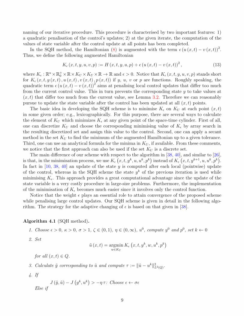
naming of our iterative procedure. This procedure is characterised by two important features: 1)a quadratic penalisation of the control’s updates; 2) at the given iterate, the computation of thevalues of state variable after the control update at all points has been completed.
In the SQH method, the Hamiltonian (8) is augmented with the term ε (u (x, t)− v (x, t))2.Thus, we define the following augmented Hamiltonian
Kε (x, t, y, u, v, p) := H (x, t, y, u, p) + ε (u (x, t)− v (x, t))2 , (13)
where Kε : Rn×R+0 ×R×KU×KU×R→ R and ε > 0. Notice that Kε (x, t, y, u, v, p) stands short
for Kε (x, t, y (x, t) , u (x, t) , v (x, t) , p (x, t)) if y, u, v or p are functions. Roughly speaking, thequadratic term ε (u (x, t)− v (x, t))2 aims at penalising local control updates that differ too muchfrom the current control value. This in turn prevents the corresponding state y to take values at(x, t) that differ too much from the current value, see Lemma 3.2. Therefore we can reasonablypursue to update the state variable after the control has been updated at all (x, t) points.
The basic idea in developing the SQH scheme is to minimise Kε on KU at each point (x, t)in some given order; e.g., lexicographically. For this purpose, there are several ways to calculatethe element of KU which minimizes Kε at any given point of the space-time cylinder. First of all,one can discretize KU and choose the corresponding minimising value of Kε by array search inthe resulting discretized set and assign this value to the control. Second, one can apply a secantmethod in the set KU to find the minimum of the augmented Hamiltonian up to a given tolerance.Third, one can use an analytical formula for the minima in KU , if available. From these comments,we notice that the first approach can also be used if the set KU is a discrete set.
The main difference of our scheme with respect to the algorithm in [38, 40], and similar to [26],is that, in the minimisation process, we use Kε
(x, t, yk, u, uk, pk
)instead of Kε
(x, t, yk+1, u, uk, pk
).
In fact in [10, 38, 40] an update of the state y is computed after each local (pointwise) updateof the control, whereas in the SQH scheme the state yk of the previous iteration is used whileminimising Kε. This approach provides a great computational advantage since the update of thestate variable is a very costly procedure in large-size problems. Furthermore, the implementationof the minimisation of Kε becomes much easier since it involves only the control function.
Notice that the weight ε plays an essential role to attain convergence of the proposed schemewhile penalising large control updates. Our SQH scheme is given in detail in the following algo-rithm. The strategy for the adaptive changing of ε is based on that given in [38].
Algorithm 4.1 (SQH method).
1. Choose ε > 0, κ > 0, σ > 1, ζ ∈ (0, 1), η ∈ (0,∞), u0, compute y0 and p0, set k ← 0
2. Setu (x, t) = argmin
w∈KUKε
(x, t, yk, w, uk, pk
)for all (x, t) ∈ Q.
3. Calculate y corresponding to u and compute τ := ‖u− uk‖2L2(Q).
4. If
J (y, u)− J(yk, uk
)> −η τ : Choose ε← σε
Else if
9

J (y, u) − J(yk, uk
)≤ −η τ : Choose ε ← ζε, yk+1 ← y, uk+1 ← u; compute pk+1
corresponding to yk+1 and uk+1 and set k ← k + 1
5. If τ < κ: STOP and return uk.Else go to 2.
Algorithm 4.1 works as follows. After choosing the problem’s parameters and an initial guessfor the control, we determine u such that the augmented Hamiltonian is minimised for a givenstate, adjoint, current control and ε. If the resulting control u and the corresponding y do notminimise the cost functional more than −ητ with respect to the former values yk and uk, weincrease ε and perform the minimisation of the resulting Kε again. Else, we accept the newcontrol function as well as the corresponding state, calculate the adjoint and diminish ε such thatgreater variations of the control value become more likely. If the convergence criterion τ < κ isnot fulfilled, then in the SQH scheme the minimisation procedure is repeated. If the convergencecriterion is fulfilled, then the algorithm stops and returns the last calculated control uk.
Next, we prove that for given x, t, y, v, p and ε there exists a u (x, t) ∈ KU that minimisesKε (x, t, y, u, v, p). Thus, Step 2 of Algorithm 4.1 is well posed. Later, we prove that there existsa ε sufficiently large such that the condition for sufficient decrease of the cost functional’s valueis satisfied, and ‖uk − uk−1‖2 decreases such that the convergence criterion is eventually satisfied.Hence, Step 4 in Algorithm 4.1 is well defined.
Concerning Step 2, we have the following.
Lemma 4.1. The function Kε : R → R, w 7→ Kε (x, t, y, w, v, p) attains a minimum for any(x, t, y, v, p) ∈ Rn × R+
0 × R×KU × R and any ε ∈ R.
Proof. As Kε is bounded from below, there is a minimising sequence (un)n∈N ⊆ KU such thatinfw∈KU Kε (x, t, y, w, v, p) = limn→∞Kε (x, t, y, un, v, p) as (Kε (x, t, y, un, v, p))n∈N is a monotoni-cally decreasing sequence and thus converging [3, II Theorem 4.1]. As KU is compact, there isa subsequence K ⊆ N such that limk→∞ uk = u with u ∈ KU . Furthermore, we have with [3, IITheorem 5.7] and [18, Theorem 3.127]
infw∈KU
Kε (x, t, y, w, v, p) = limk→∞
Kε (x, t, y, uk, v, p) = lim infk→∞
Kε (x, t, y, uk, v, p)
= lim infk→∞
(1
2(y − yd)2 +
α
2u2k + γg (uk) + puk + ε (uk − v)2
)≥ 1
2(y − yd)2 +
α
2u2 + γg (u) + pu+ ε (u− v)2 = Kε (x, t, y, u, v, p)
(14)
because of the lower semi-continuity of g.
The question arises whether u, obtained in Step 2, is Lebesgue measurable. This is certainlythe case if the function (z, u) 7→ Kε (z, y (z) , u, v (z) , p (z)) is Lebesgue measurable in z := (x, t)for each u ∈ KU and is continuous in u for each z ∈ Q. For this case, see [37, 14.29 Example,14.37 Theorem].
If Kε is only lower semi-continuous in u for each z ∈ Q, then, in general, we cannot guaranteethat u is Lebesgue measurable; see also the paragraph following [37, 14.28 Proposition]. However,
in the case of g (u) :=
|u− d| for |u− d| > s
0 otherwise, d ∈ R, s > 0, as considered in the section on
10

numerical experiments, we can prove that starting our SQH scheme with an initial guess u0 thatis Lebesgue measurable, we obtain iterates uk that are Lebesgue measurable, see Section 5 fordetails. For the remaining part of this section, we assume that u, which is generated in Step 2 ofAlgorithm 4.1, is measurable.
In order to prove that, by increasing ε in Step 4 of Algorithm 4.1 (ε← σε), a ε is obtained suchthat the condition for sufficient decrease is satisfied, we present the following lemma. A similarresult is proved in [10].
Lemma 4.2. Let (y, u) and(yk, uk
)be generated by Algorithm 4.1, k ∈ N0, and u, uk be measur-
able; denote δu := u − uk. Then, there is a θ > 0 independent of ε such that for ε > 0 currentlychosen by Algorithm 4.1, the following holds
J (y, u)− J(yk, uk
)≤ − (ε− θ) ‖δu‖2
L2(Q). (15)
In particular, J (y, u)− J(yk, uk
)≤ 0 for ε ≥ θ.
Proof. We denote δy := y − yk. In this proof, we have as in Algorithm 4.1 thatKε
(x, t, yk, u, uk, pk
)≤ Kε
(x, t, yk, w, uk, pk
)for all w ∈ KU , and thus
Kε
(x, t, yk, u, uk, pk
)≤ Kε
(x, t, yk, uk, uk, pk
)= H
(x, t, yk, uk, pk
)for all (x, t) ∈ Q. To obtain (15), we perform the following estimates where we use the Taylorexpansion of the map y 7→ H (·, ·, y, ·, ·), see [4, Chapter VII, Theorem 5.8 and Remark 5.9] and[4, Chapter VII, Theorem 5.2]
J (y, u)− J(yk, uk
)=
∫Q
F (x, t, y, u)− F(x, t, yk, uk
)dxdt
=
∫Q
F (x, t, y, u) + pku− pku− F(x, t, yk, uk
)− pkuk + pkukdxdt
=
∫Q
H(x, t, y, u, pk
)− pku−H
(x, t, yk, uk, pk
)+ pkukdxdt
=
∫Q
H(x, t, yk + δy, u, pk
)−H
(x, t, yk, uk, pk
)+ pk
(uk − u
)dxdt
=
∫Q
H(x, t, yk, u, pk
)+(yk − yd
)δy +
1
2(δy)2 −H
(x, t, yk, uk, pk
)dxdt
+
∫Q
pk(uk − u
)dxdt
=
∫Q
Kε
(x, t, yk, u, uk, pk
)− ε (δu)2 −H
(x, t, yk, uk, pk
)+
1
2(δy)2 dxdt
+
∫ T
0
−((pk)′, δy)
+D(∇pk,∇δy
)−(
(δy)′, pk)−D
(∇δy,∇pk
)dt
≤∫Q
−ε (δu)2 +1
2(δy)2 dxdt.
11

Notice that in the first before last step, we use integration by parts [44, Theorem 3.11] using the factthat δy (·, 0) = 0 and pk (·, T ) = 0, because of the initial condition for the state and the terminalcondition for the adjoint, respectively. We have that ‖δy (·, t) ‖2
L2(Ω) ≤ c (D) ‖δu (·, t) ‖2L2(Ω) for all
t ∈ [0, T ], c (D) > 0. This can be seen as follows; similar to [28, (6.3)]. Consider the differencebetween (1) with u← u and y ← y and the same equation (1) but with u← uk and y ← yk. Weobtain ∫ T
0
∫Ω
δy′ (x, t) v (x) +D∇δy (x, t)∇v (x) dxdt =
∫ T
0
∫Ω
δu (x, t) v (x) dxdt,
from which we have∫ T
0
1
2
d
dt‖δy (·, t) ‖2
L2(Ω) +D‖∇δy (·, t) ‖2L2(Ω)dt ≤
∫ T
0
||δu (·, t) ‖2L2(Ω)‖δy (·, t) ‖2
L2(Ω)dt,
according to [19, page 287, Theorem 3] and the Cauchy-Schwarz inequality, see [2, (2.2)]. Next,we have
1
2
(‖δy (·, T ) ‖2
L2(Ω) − ‖δy (·, 0) ‖2L2(Ω)
)+D‖∇δy‖2
L2(Q) ≤ c
∫ T
0
||δu (·, t) ‖2L2(Ω) ‖∇δy (·, t) ‖2
L2(Ω)dt,
for some c > 0. Thus, as ‖δy (·, 0) ‖2L2(Ω) = 0, we obtain
‖∇δy‖L2(Q) ≤ c (D) ‖δu‖L2(Q),
for some c (D) ≥ 0. Furthermore, by the Poincare inequality [2, (6.7)], we have for c > 0
‖δy‖L2(Q) =
√∫ T
0
‖δy‖2L2(Ω)dt ≤ c
√∫ T
0
‖∇δy‖2L2(Ω)dt = c‖∇δy‖L2(Q) ≤ c (D) ‖δu‖L2(Q).
Thus, we have
‖δy‖2L2(Q) =
∫ T
0
∫Ω
(δy)2 dxdt =
∫ T
0
‖δy (·, t) ‖2L2(Ω)dt ≤ c (D)
∫ T
0
‖δu (·, t) ‖2L2(Ω)dt
= c (D) ‖δu‖2L2(Q).
We conclude as follows∫Q
−ε (δu)2 +1
2(δy)2 dxdt = −ε‖δu‖2
L2(Q) +1
2‖δy‖2
L2(Q) ≤(−ε+
1
2c (D)
)‖δu‖2
L2(Q),
which proves the claim with θ := c(D)2
.
Next, we prove a lemma stating that Algorithm 4.1 stops when uk is a solution to (12).
Lemma 4.3. Let yk and uk be generated by Algorithm 4.1, k ∈ N0, and uk be measurable. If theiterate uk is optimal, then Algorithm 4.1 stops, returning uk.
12
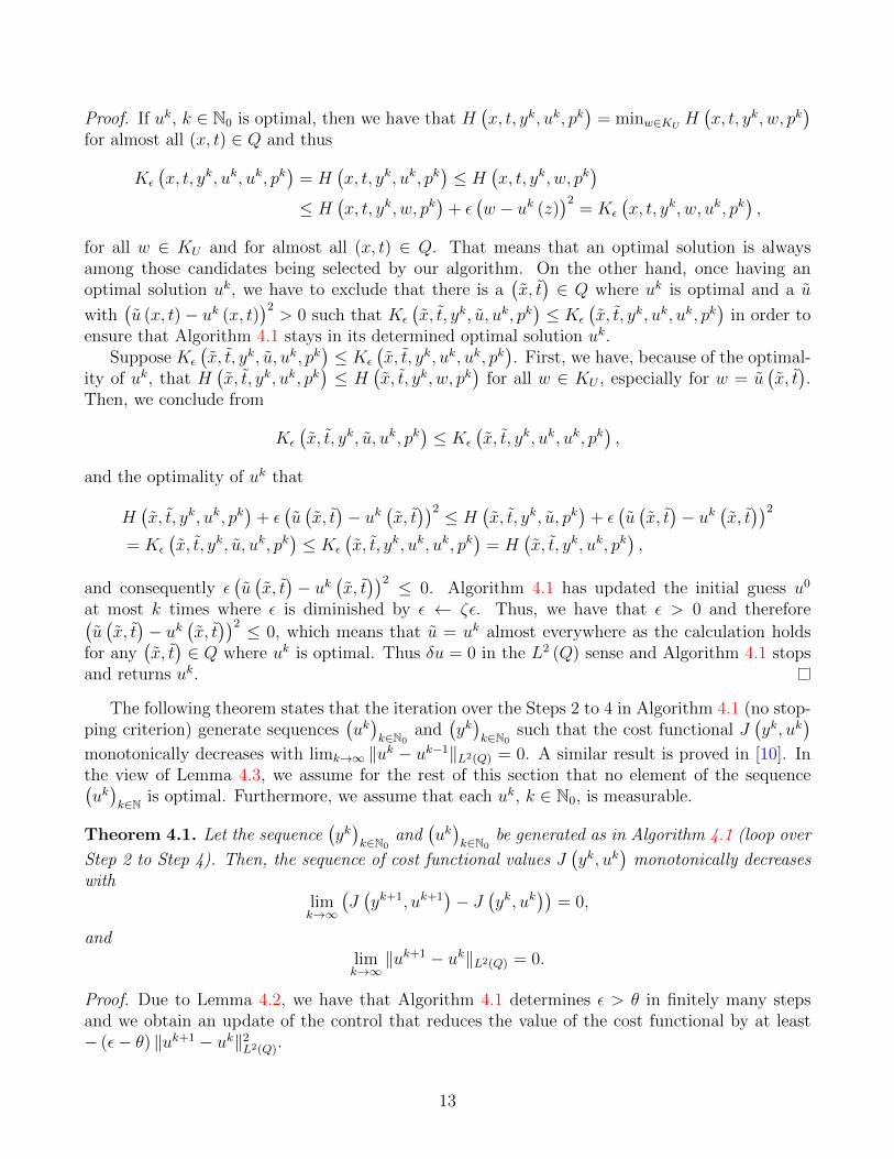
Proof. If uk, k ∈ N0 is optimal, then we have that H(x, t, yk, uk, pk
)= minw∈KU H
(x, t, yk, w, pk
)for almost all (x, t) ∈ Q and thus
Kε
(x, t, yk, uk, uk, pk
)= H
(x, t, yk, uk, pk
)≤ H
(x, t, yk, w, pk
)≤ H
(x, t, yk, w, pk
)+ ε(w − uk (z)
)2= Kε
(x, t, yk, w, uk, pk
),
for all w ∈ KU and for almost all (x, t) ∈ Q. That means that an optimal solution is alwaysamong those candidates being selected by our algorithm. On the other hand, once having anoptimal solution uk, we have to exclude that there is a
(x, t)∈ Q where uk is optimal and a u
with(u (x, t)− uk (x, t)
)2> 0 such that Kε
(x, t, yk, u, uk, pk
)≤ Kε
(x, t, yk, uk, uk, pk
)in order to
ensure that Algorithm 4.1 stays in its determined optimal solution uk.Suppose Kε
(x, t, yk, u, uk, pk
)≤ Kε
(x, t, yk, uk, uk, pk
). First, we have, because of the optimal-
ity of uk, that H(x, t, yk, uk, pk
)≤ H
(x, t, yk, w, pk
)for all w ∈ KU , especially for w = u
(x, t).
Then, we conclude from
Kε
(x, t, yk, u, uk, pk
)≤ Kε
(x, t, yk, uk, uk, pk
),
and the optimality of uk that
H(x, t, yk, uk, pk
)+ ε(u(x, t)− uk
(x, t))2 ≤ H
(x, t, yk, u, pk
)+ ε(u(x, t)− uk
(x, t))2
= Kε
(x, t, yk, u, uk, pk
)≤ Kε
(x, t, yk, uk, uk, pk
)= H
(x, t, yk, uk, pk
),
and consequently ε(u(x, t)− uk
(x, t))2 ≤ 0. Algorithm 4.1 has updated the initial guess u0
at most k times where ε is diminished by ε ← ζε. Thus, we have that ε > 0 and therefore(u(x, t)− uk
(x, t))2 ≤ 0, which means that u = uk almost everywhere as the calculation holds
for any(x, t)∈ Q where uk is optimal. Thus δu = 0 in the L2 (Q) sense and Algorithm 4.1 stops
and returns uk.
The following theorem states that the iteration over the Steps 2 to 4 in Algorithm 4.1 (no stop-ping criterion) generate sequences
(uk)k∈N0
and(yk)k∈N0
such that the cost functional J(yk, uk
)monotonically decreases with limk→∞ ‖uk − uk−1‖L2(Q) = 0. A similar result is proved in [10]. Inthe view of Lemma 4.3, we assume for the rest of this section that no element of the sequence(uk)k∈N is optimal. Furthermore, we assume that each uk, k ∈ N0, is measurable.
Theorem 4.1. Let the sequence(yk)k∈N0
and(uk)k∈N0
be generated as in Algorithm 4.1 (loop over
Step 2 to Step 4). Then, the sequence of cost functional values J(yk, uk
)monotonically decreases
withlimk→∞
(J(yk+1, uk+1
)− J
(yk, uk
))= 0,
andlimk→∞‖uk+1 − uk‖L2(Q) = 0.
Proof. Due to Lemma 4.2, we have that Algorithm 4.1 determines ε > θ in finitely many stepsand we obtain an update of the control that reduces the value of the cost functional by at least− (ε− θ) ‖uk+1 − uk‖2
L2(Q).
13
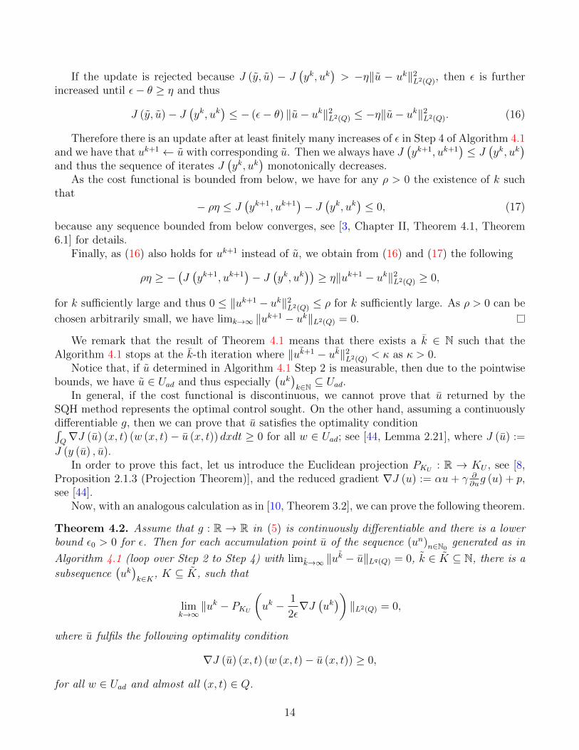
If the update is rejected because J (y, u) − J(yk, uk
)> −η‖u − uk‖2
L2(Q), then ε is furtherincreased until ε− θ ≥ η and thus
J (y, u)− J(yk, uk
)≤ − (ε− θ) ‖u− uk‖2
L2(Q) ≤ −η‖u− uk‖2L2(Q). (16)
Therefore there is an update after at least finitely many increases of ε in Step 4 of Algorithm 4.1and we have that uk+1 ← u with corresponding u. Then we always have J
(yk+1, uk+1
)≤ J
(yk, uk
)and thus the sequence of iterates J
(yk, uk
)monotonically decreases.
As the cost functional is bounded from below, we have for any ρ > 0 the existence of k suchthat
− ρη ≤ J(yk+1, uk+1
)− J
(yk, uk
)≤ 0, (17)
because any sequence bounded from below converges, see [3, Chapter II, Theorem 4.1, Theorem6.1] for details.
Finally, as (16) also holds for uk+1 instead of u, we obtain from (16) and (17) the following
ρη ≥ −(J(yk+1, uk+1
)− J
(yk, uk
))≥ η‖uk+1 − uk‖2
L2(Q) ≥ 0,
for k sufficiently large and thus 0 ≤ ‖uk+1 − uk‖2L2(Q) ≤ ρ for k sufficiently large. As ρ > 0 can be
chosen arbitrarily small, we have limk→∞ ‖uk+1 − uk‖L2(Q) = 0.
We remark that the result of Theorem 4.1 means that there exists a k ∈ N such that theAlgorithm 4.1 stops at the k-th iteration where ‖uk+1 − uk‖2
L2(Q) < κ as κ > 0.Notice that, if u determined in Algorithm 4.1 Step 2 is measurable, then due to the pointwise
bounds, we have u ∈ Uad and thus especially(uk)k∈N ⊆ Uad.
In general, if the cost functional is discontinuous, we cannot prove that u returned by theSQH method represents the optimal control sought. On the other hand, assuming a continuouslydifferentiable g, then we can prove that u satisfies the optimality condition∫Q∇J (u) (x, t) (w (x, t)− u (x, t)) dxdt ≥ 0 for all w ∈ Uad; see [44, Lemma 2.21], where J (u) :=
J (y (u) , u).In order to prove this fact, let us introduce the Euclidean projection PKU : R → KU , see [8,
Proposition 2.1.3 (Projection Theorem)], and the reduced gradient ∇J (u) := αu + γ ∂∂ug (u) + p,
see [44].Now, with an analogous calculation as in [10, Theorem 3.2], we can prove the following theorem.
Theorem 4.2. Assume that g : R → R in (5) is continuously differentiable and there is a lowerbound ε0 > 0 for ε. Then for each accumulation point u of the sequence (un)n∈N0
generated as in
Algorithm 4.1 (loop over Step 2 to Step 4) with limk→∞ ‖uk − u‖Lq(Q) = 0, k ∈ K ⊆ N, there is a
subsequence(uk)k∈K, K ⊆ K, such that
limk→∞‖uk − PKU
(uk − 1
2ε∇J
(uk))‖L2(Q) = 0,
where u fulfils the following optimality condition
∇J (u) (x, t) (w (x, t)− u (x, t)) ≥ 0,
for all w ∈ Uad and almost all (x, t) ∈ Q.
14
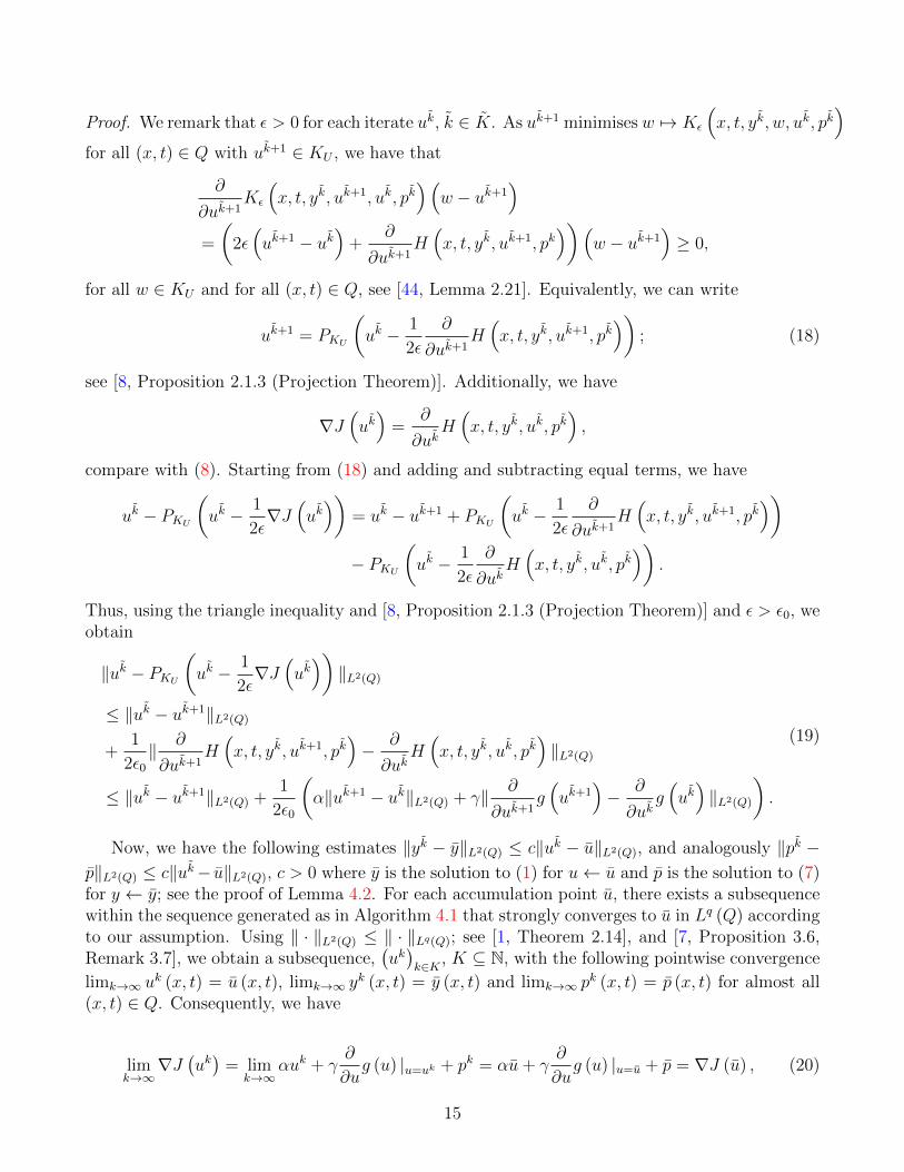
Proof. We remark that ε > 0 for each iterate uk, k ∈ K. As uk+1 minimises w 7→ Kε
(x, t, yk, w, uk, pk
)for all (x, t) ∈ Q with uk+1 ∈ KU , we have that
∂
∂uk+1Kε
(x, t, yk, uk+1, uk, pk
)(w − uk+1
)=
(2ε(uk+1 − uk
)+
∂
∂uk+1H(x, t, yk, uk+1, pk
))(w − uk+1
)≥ 0,
for all w ∈ KU and for all (x, t) ∈ Q, see [44, Lemma 2.21]. Equivalently, we can write
uk+1 = PKU
(uk − 1
2ε
∂
∂uk+1H(x, t, yk, uk+1, pk
)); (18)
see [8, Proposition 2.1.3 (Projection Theorem)]. Additionally, we have
∇J(uk)
=∂
∂ukH(x, t, yk, uk, pk
),
compare with (8). Starting from (18) and adding and subtracting equal terms, we have
uk − PKU(uk − 1
2ε∇J
(uk))
= uk − uk+1 + PKU
(uk − 1
2ε
∂
∂uk+1H(x, t, yk, uk+1, pk
))− PKU
(uk − 1
2ε
∂
∂ukH(x, t, yk, uk, pk
)).
Thus, using the triangle inequality and [8, Proposition 2.1.3 (Projection Theorem)] and ε > ε0, weobtain
‖uk − PKU(uk − 1
2ε∇J
(uk))‖L2(Q)
≤ ‖uk − uk+1‖L2(Q)
+1
2ε0‖ ∂
∂uk+1H(x, t, yk, uk+1, pk
)− ∂
∂ukH(x, t, yk, uk, pk
)‖L2(Q)
≤ ‖uk − uk+1‖L2(Q) +1
2ε0
(α‖uk+1 − uk‖L2(Q) + γ‖ ∂
∂uk+1g(uk+1
)− ∂
∂ukg(uk)‖L2(Q)
).
(19)
Now, we have the following estimates ‖yk − y‖L2(Q) ≤ c‖uk − u‖L2(Q), and analogously ‖pk −p‖L2(Q) ≤ c‖uk− u‖L2(Q), c > 0 where y is the solution to (1) for u← u and p is the solution to (7)for y ← y; see the proof of Lemma 4.2. For each accumulation point u, there exists a subsequencewithin the sequence generated as in Algorithm 4.1 that strongly converges to u in Lq (Q) accordingto our assumption. Using ‖ · ‖L2(Q) ≤ ‖ · ‖Lq(Q); see [1, Theorem 2.14], and [7, Proposition 3.6,Remark 3.7], we obtain a subsequence,
(uk)k∈K , K ⊆ N, with the following pointwise convergence
limk→∞ uk (x, t) = u (x, t), limk→∞ y
k (x, t) = y (x, t) and limk→∞ pk (x, t) = p (x, t) for almost all
(x, t) ∈ Q. Consequently, we have
limk→∞∇J
(uk)
= limk→∞
αuk + γ∂
∂ug (u) |u=uk + pk = αu+ γ
∂
∂ug (u) |u=u + p = ∇J (u) , (20)
15
for almost every (x, t) ∈ Q. If we take the limit on both sides of (19), considering the pointwiseconverging subsequence, we obtain
limk→∞‖uk − PKU
(uk − 1
2ε∇J
(uk))‖L2(Q) = 0, (21)
where we use Theorem 4.1 for the first and second term and the dominated convergence theorem[7, Proposition 2.17], [7, 2.2 Measurable and Borel functions] and [3, III.3 Theorem 3.6] with thebounded image of uk, k ∈ K for the last term.
Next, we prove that∇J (u) (x, t) (w (x, t)− u (x, t)) ≥ 0 for all w ∈ Uad for almost all (x, t) ∈ Q.For this purpose, we start with
vk := PKU
(uk − 1
2ε∇J
(uk))
,
for almost every (x, t) ∈ Q. This is equivalent to(vk − uk +
1
2ε∇J
(uk)) (
w − vk)≥ 0,
for all w ∈ Uad for almost all (x, t) ∈ Q, see [8, Proposition 2.1.3 (Projection Theorem)]. Then wehave (
vk − uk) (w − vk
)+
1
2ε∇J
(uk) (w − vk
)≥ 0.
Adding and subtracting uk, we obtain
2ε(vk − uk
) (w − vk
)+∇J
(uk) (w − uk
)+∇J
(uk) (uk − vk
)≥ 0. (22)
Due to |w − vk| ≤ 2 max (|ua|, |ub|) and the upper bound σ (η + θ) for ε because of (16) and Step4 of Algorithm 4.1, and the fact that converging sequences are bounded [3, II, Theorem 1.10]combined with (21) and (20), we obtain the following by taking the limit in (22). We have
∇J (u) (w − u) ≥ 0,
for all w ∈ Uad for almost all (x, t) ∈ Q; see [3, II Theorem 2.4] and [3, II Theorem 2.7].
This result also proves that∫Q∇J (u) (x, t) (w (x, t)− u (x, t)) dxdt ≥ 0 for all w ∈ Uad, see
[5, Chapter X Corollary 2.16]. Notice that, if g is strictly convex, then u is the optimal controlsought.
We remark that the analysis above is performed at a functional level and independently of thediscretisation used. However, for the numerical realisation of our optimisation scheme, we considerthe following finite differences setting [25], where we assume that the control is approximated bya piecewise constant function.
We take a space-time cylinder Q = Ω × (0, T ) with Ω = (a, b)n, and define the followingspace-time grid
Qh,4t := (xi1...in , tm) , | xi1...in ∈ Ωh, tm = m4t, m ∈ 1, ..., Nt ,
16

whereΩh = (a+ i1h, . . . , a+ inh) ∈ Rn, ij ∈ 1, ..., N − 1 , j ∈ 1, ..., n .
The space and time mesh-sizes are given by h := b−aN
, 4t := TNt
. We assume that the grid points(xi1...in , tm) and tm = m4t are ordered lexicographically.
In order to compute the state and adjoint variables, we approximate (1) and (7) using theimplicit Euler scheme and finite differences. For the computation of the integrals appearing in Jand for the integration of H (see below), we use the rectangle rule; see, e.g., [41].
5 Numerical experiments
In this section, we present results of numerical experiments to validate our optimal control formu-lation and the convergence performance of the SQH method.
For the lower semi-continuous function g in (3), we choose the following
gd,s (u) :=
|u− d| for |u− d| > s
0 otherwise .(23)
Notice that Gd,s (u) :=∫Qgd,s (u (x, t)) dxdt measures zero costs as far as the control u is in
the L1 closed ball centered in d ∈ R with radius s > 0. If u is in the complement of this ball, thenthe cost given by Gd,s is of L1 type. It can be shown with an elementary calculation that Gd,s isa discontinuous functional (e.g., consider the case of constant controls).
In our numerical experiments, we consider Ω = (a, b) with a = 0, b = 1 and T = 1. Theinitial guess for the control and the initial value y0 for the state is the zero function. Furthermore,κ = 10−6, ζ = 3
20, σ = 50 and η = 10−7. The initial value of ε equals 3
5.
The numerical parameters are set as follows, N = 100, Nt = 200, D = 15, and if not otherwise
stated α = 10−5, γ = 10−1. Furthermore, we have, KU = [0, 10] and
yd (x, t) =
5 if x (t)− c ≤ x ≤ x (t) + c
0 else,(24)
where x (t) := x0+ 25
(b− a) sin(2π t
T
), x0 = b+a
2, and c = 7
100(b− a). We choose the cost functional
J as in (3) - (4) with the desired trajectory (24) and set d = 0, s = 1.The augmented Hamiltonian Kε (x, t, y, u, v, p) is minimised as follows. As y and p are held
fixed, we have
Kε (x, t, y, u, v, p) :=α
2u2 + g0,1 (u) + pu+ ε (u− v)2 .
Its minimum can be exactly given by a case study as follows.If 0 ≤ u ≤ s, we have Kε (x, t, y, u, v, p) = α
2u2 + pu+ ε (u− v)2 with its minimum at
u1 := min
(max
(0,
2εv − p2ε+ α
), s
).
If s < u ≤ 10, we have Kε (x, t, y, u, v, p) := α2u2 + γu+ pu+ ε (u− v)2 with its minimum at
u2 := min
(max
(s,
2εv − (p+ γ)
2ε+ α
), 10
).
17

Then the minimum of Kε over KU is given by
u = argminw∈KU
Kε (x, t, y, w, v, p) = argminw∈u1,u2
Kε (x, t, y, w, v, p) .
Next, we remark that u, as a function, is Lebesgue measurable assuming that the last iteratev is also Lebesgue measurable. To illustrate this fact, denote with z := (x, t), and notice thatp is Lebesgue measurable since it is the solution to (10). Thus, we have that u1 and u2 areLebesgue measurable functions; see [15, Proposition 2.1.4, Proposition 2.1.7]. Further, we havethat Kε (z, u1 (z)) := Kε (z, y (z) , u1 (z) , v (z) , p (z)) andKε (z, u1 (z)) := Kε (z, y (z) , u1 (z) , v (z) , p (z)) are Lebesgue measurable according to Lemma6.3 in the Appendix and because the sum and the product of Lebesgue measurable functions isLebesgue measurable; see [15, Proposition 2.1.7].
Now, the function u (z) is given by
u (z) :=
u1 (z) if Kε (z, u1 (z)) ≤ Kε (z, u2 (z))
u2 (z) if Kε (z, u1 (z)) > Kε (z, u2 (z)).
According to [15, Proposition 2.1.1] and the following paragraph, u is Lebesgue measurable if andonly if the set z ∈ Q| u (z) > c is Lebesgue measurable for any c ∈ R. To show this fact, noticethat the following holds
z ∈ Q| u (z) > c =(z ∈ Q| u1 (z) > c ∩
z ∈ Q| Kε (z, u1 (z)) ≤ Kε (z, u2 (z))
)∪(z ∈ Q| u2 (z) > c ∩
z ∈ Q| Kε (z, u1 (z)) > Kε (z, u2 (z))
).
(25)
Thus u is Lebesgue measurable, as the intersection and union of finite Lebesgue measurablesets is Lebesgue measurable, see [5, IX Theorem 5.1, Remark 1.1], if and only if the singlesets are measurable. Now, we have that the sets z ∈ Q| u1 (z) > c and z ∈ Q| u2 (z) > care Lebesgue measurable for any c ∈ R as u1 and u2 are Lebesgue measurable; further the setz ∈ Q| Kε (z, u1 (z)) ≤ Kε (z, u2 (z))
is Lebesgue measurable, see [15, Proposition 2.1.3], and
z ∈ Q| Kε (z, u1 (z)) > Kε (z, u2 (z))
= Q\z ∈ Q| Kε (z, u1 (z)) ≤ Kε (z, u2 (z))
is Lebesgue measurable according to [5, IX Remark 1.1].
Next, having completed the theoretical discussion, we perform the first set of experimentsusing Algorithm 4.1 to solve our optimal control problem. The SQH algorithm converges in 29iterations and we obtain the state and control functions depicted in Figure 1. The plot of thecontrol function shows clearly the action of the discontinuous cost of the control given by g0,1 andthe presence of the control’s upper bound at 10.
18

10
0.2
1
0.4
0.8
0.6
0.8
x
0.50.6
1
t
1.2
0.40.2
00
(a) The state y
10
1
2
4
0.8
6
x
0.5
8
0.6
t
10
0.40.2
00
(b) The control function u
10
1
1
2
0.8
3
x
0.5
4
0.6
t
5
0.40.2
00
(c) The desired function yd
Figure 1: Optimal solution for the first experiment setting.
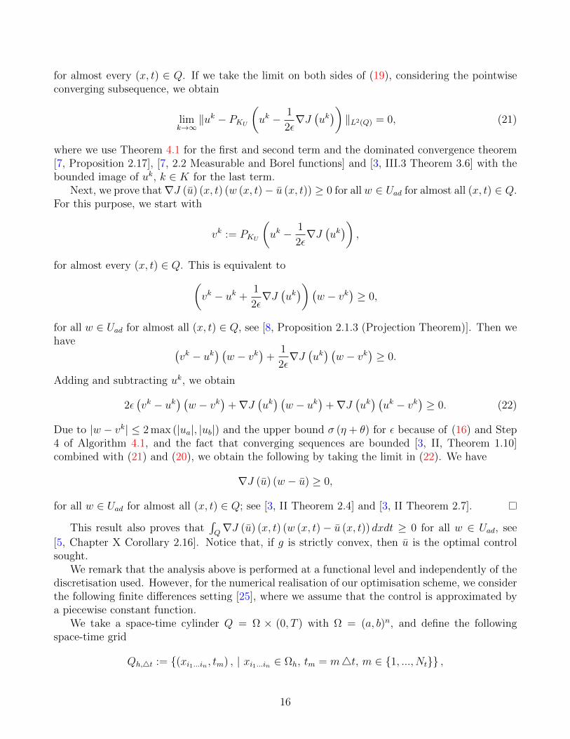
With the second experiment, we present results to investigate how well the solution of theSQH method satisfies the optimality condition given by the PMP. For this purpose, in Table 1 wereport the values of
∆H = max(x,t)∈Qh,4t
(H (x, t, y, u, p)− min
w∈KUH (x, t, y, w, p)
).
The value of ∆H gives a measure of optimality of the SQH solution (y, u, p) and the resultsreported in Table 1 demonstrate how ∆H decreases as we refine the mesh size and the value of κ,thus demonstrating an improvement in accuracy of the PMP solution by refinement.
In Table 2, we report results that aim at showing the ratio of numbers of grid points (x, t) ∈Qh,4t where the optimality condition is satisfied to machine precision. For this purpose, in Table2, we give the ratio of grid points where the following holds
H (x, t, y, u, p)− minw∈KU
H (x, t, y, w, p) ≈ eps,
19
with eps the machine precision given by 2.2 · 10−16 in our case. We see that, independently of themesh size, at almost all grid points the PMP condition is fulfilled to machine precision, alreadyfor κ = 10−6.
Nt ×Nκ
10−1 10−3 10−6 10−11 10−16
100× 200 3.43 9.00 · 10−3 5.68 · 10−3 1.27 · 10−3 7.29 · 10−4
200× 400 3.42 5.34 · 10−3 5.17 · 10−4 5.17 · 10−4 5.17 · 10−4
400× 800 3.41 1.06 · 10−2 6.89 · 10−3 6.70 · 10−4 6.70 · 10−4
800× 1600 3.41 1.13 · 10−2 3.93 · 10−7 1.82 · 10−10 7.08 · 10−11
Table 1: Values of ∆H of the SQH solution with different choices of the value of κ.
Nt ×Nκ
10−1 10−3 10−6 10−11 10−16
100× 200 0 0.9973 0.9988 0.9995 0.9998200× 400 6.28 · 10−5 0.9966 0.9998 0.9998 0.9998400× 800 6.70 · 10−4 0.9934 0.9981 0.9998 0.9998800× 1600 1.59 · 10−3 0.9868 0.9998 0.9998 0.9998
Table 2: Ratio of grid points at which the Pontryagin maximum principle is fulfilled to machineprecision to the total number of grid points.
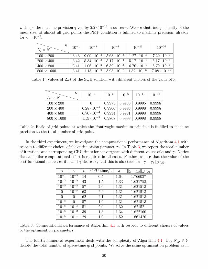
In the third experiment, we investigate the computational performance of Algorithm 4.1 withrespect to different choices of the optimisation parameters. In Table 3, we report the total numberof iterations and corresponding CPU times for convergence with different values of α and γ. Noticethat a similar computational effort is required in all cases. Further, we see that the value of thecost functional decreases if α and γ decrease, and this is also true for ‖y − yd‖L2(Q).
α γ k CPU time/s J ||y − yd||L2(Q)
10−1 10−5 14 0.5 1.64 1.76603710−3 10−5 43 1.5 1.33 1.62175310−5 10−5 57 2.0 1.31 1.621513
0 10−5 63 2.2 1.31 1.6215130 0 62 2.1 1.31 1.621513
10−5 0 57 1.9 1.31 1.62151310−5 10−3 51 2.0 1.32 1.62152110−5 10−2 39 1.3 1.34 1.62216010−5 10−1 29 1.0 1.52 1.661420
Table 3: Computational performance of Algorithm 4.1 with respect to different choices of valuesof the optimisation parameters.
The fourth numerical experiment deals with the complexity of Algorithm 4.1. Let Ngp ∈ Ndenote the total number of space-time grid points. We solve the same optimisation problem as in
20
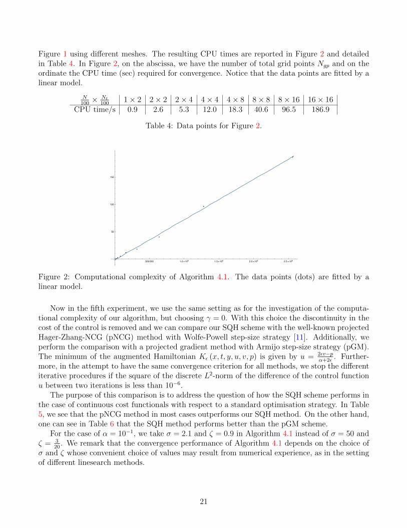
Figure 1 using different meshes. The resulting CPU times are reported in Figure 2 and detailedin Table 4. In Figure 2, on the abscissa, we have the number of total grid points Ngp and on theordinate the CPU time (sec) required for convergence. Notice that the data points are fitted by alinear model.
N100× Nt
1001× 2 2× 2 2× 4 4× 4 4× 8 8× 8 8× 16 16× 16
CPU time/s 0.9 2.6 5.3 12.0 18.3 40.6 96.5 186.9
Table 4: Data points for Figure 2.
500 000 1.0×10⁶
1.5×10⁶
2.0×10⁶
2.5×10⁶
50
100
150
Figure 2: Computational complexity of Algorithm 4.1. The data points (dots) are fitted by alinear model.
Now in the fifth experiment, we use the same setting as for the investigation of the computa-tional complexity of our algorithm, but choosing γ = 0. With this choice the discontinuity in thecost of the control is removed and we can compare our SQH scheme with the well-known projectedHager-Zhang-NCG (pNCG) method with Wolfe-Powell step-size strategy [11]. Additionally, weperform the comparison with a projected gradient method with Armijo step-size strategy (pGM).The minimum of the augmented Hamiltonian Kε (x, t, y, u, v, p) is given by u = 2εv−p
α+2ε. Further-
more, in the attempt to have the same convergence criterion for all methods, we stop the differentiterative procedures if the square of the discrete L2-norm of the difference of the control functionu between two iterations is less than 10−6.
The purpose of this comparison is to address the question of how the SQH scheme performs inthe case of continuous cost functionals with respect to a standard optimisation strategy. In Table5, we see that the pNCG method in most cases outperforms our SQH method. On the other hand,one can see in Table 6 that the SQH method performs better than the pGM scheme.
For the case of α = 10−1, we take σ = 2.1 and ζ = 0.9 in Algorithm 4.1 instead of σ = 50 andζ = 3
20. We remark that the convergence performance of Algorithm 4.1 depends on the choice of
σ and ζ whose convenient choice of values may result from numerical experience, as in the settingof different linesearch methods.
21
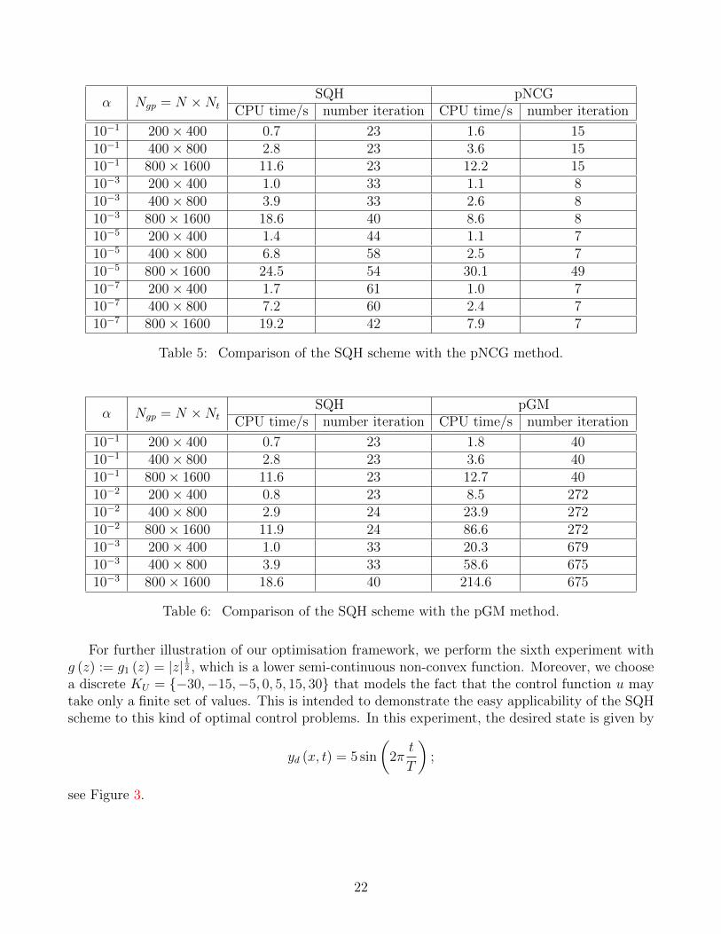
α Ngp = N ×NtSQH pNCG
CPU time/s number iteration CPU time/s number iteration
10−1 200× 400 0.7 23 1.6 1510−1 400× 800 2.8 23 3.6 1510−1 800× 1600 11.6 23 12.2 1510−3 200× 400 1.0 33 1.1 810−3 400× 800 3.9 33 2.6 810−3 800× 1600 18.6 40 8.6 810−5 200× 400 1.4 44 1.1 710−5 400× 800 6.8 58 2.5 710−5 800× 1600 24.5 54 30.1 4910−7 200× 400 1.7 61 1.0 710−7 400× 800 7.2 60 2.4 710−7 800× 1600 19.2 42 7.9 7
Table 5: Comparison of the SQH scheme with the pNCG method.
α Ngp = N ×NtSQH pGM
CPU time/s number iteration CPU time/s number iteration
10−1 200× 400 0.7 23 1.8 4010−1 400× 800 2.8 23 3.6 4010−1 800× 1600 11.6 23 12.7 4010−2 200× 400 0.8 23 8.5 27210−2 400× 800 2.9 24 23.9 27210−2 800× 1600 11.9 24 86.6 27210−3 200× 400 1.0 33 20.3 67910−3 400× 800 3.9 33 58.6 67510−3 800× 1600 18.6 40 214.6 675
Table 6: Comparison of the SQH scheme with the pGM method.
For further illustration of our optimisation framework, we perform the sixth experiment withg (z) := g1 (z) = |z| 12 , which is a lower semi-continuous non-convex function. Moreover, we choosea discrete KU = −30,−15,−5, 0, 5, 15, 30 that models the fact that the control function u maytake only a finite set of values. This is intended to demonstrate the easy applicability of the SQHscheme to this kind of optimal control problems. In this experiment, the desired state is given by
yd (x, t) = 5 sin
(2π
t
T
);
see Figure 3.
22
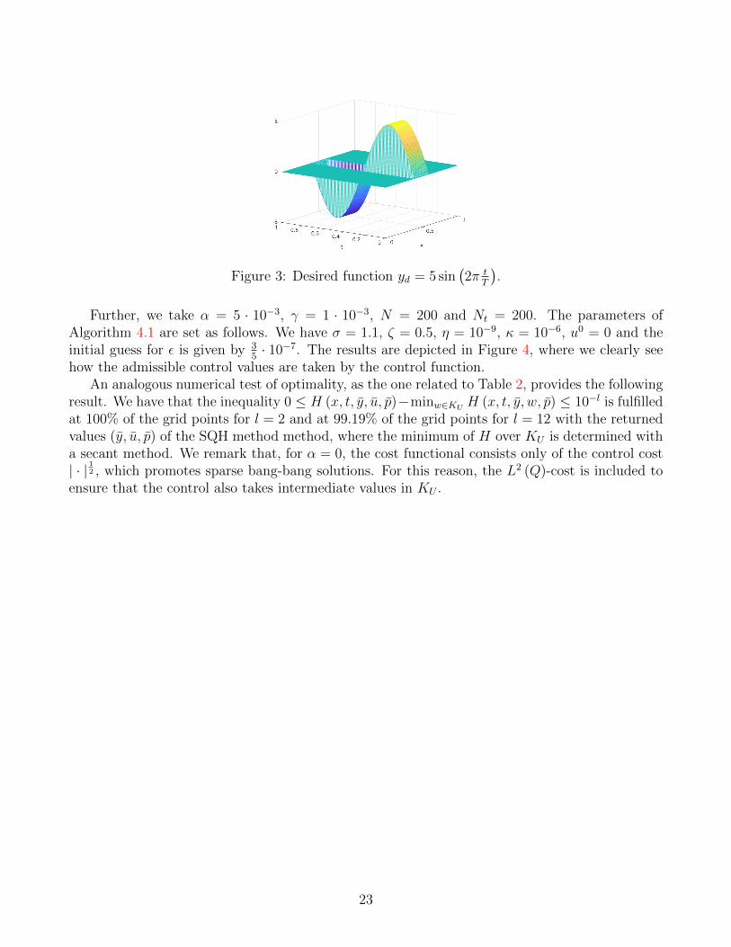
Figure 3: Desired function yd = 5 sin(2π t
T
).
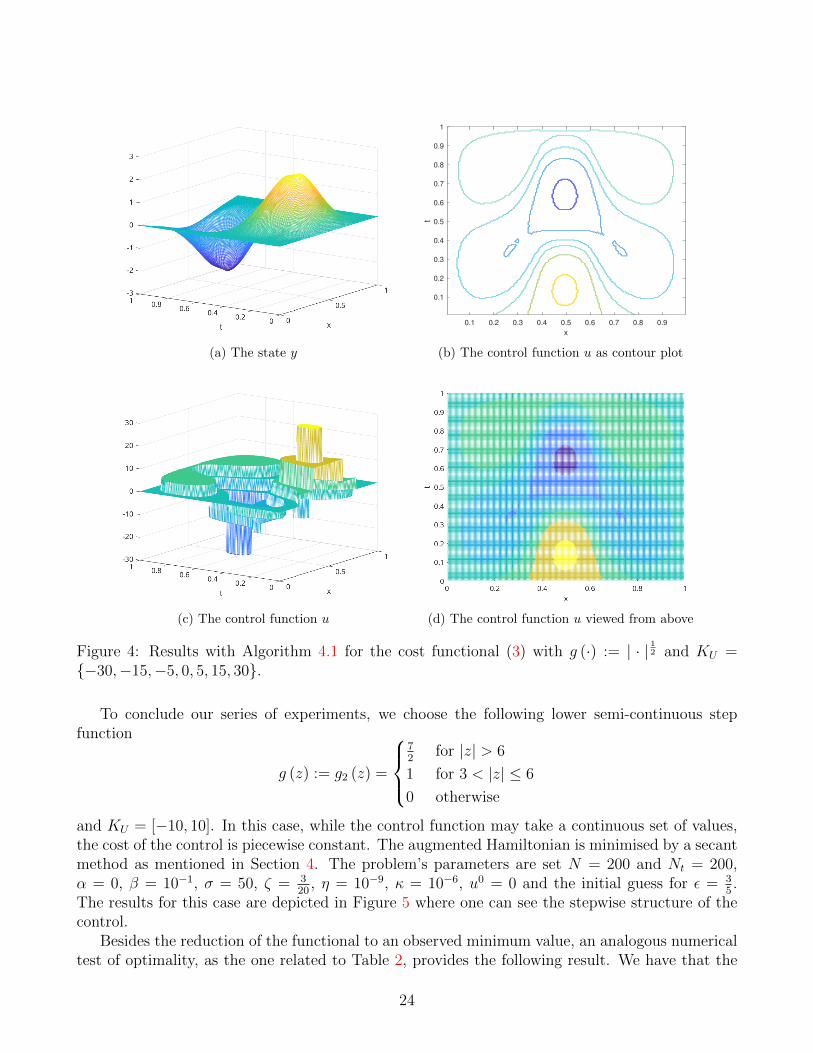
Further, we take α = 5 · 10−3, γ = 1 · 10−3, N = 200 and Nt = 200. The parameters ofAlgorithm 4.1 are set as follows. We have σ = 1.1, ζ = 0.5, η = 10−9, κ = 10−6, u0 = 0 and theinitial guess for ε is given by 3
5· 10−7. The results are depicted in Figure 4, where we clearly see
how the admissible control values are taken by the control function.An analogous numerical test of optimality, as the one related to Table 2, provides the following
result. We have that the inequality 0 ≤ H (x, t, y, u, p)−minw∈KU H (x, t, y, w, p) ≤ 10−l is fulfilledat 100% of the grid points for l = 2 and at 99.19% of the grid points for l = 12 with the returnedvalues (y, u, p) of the SQH method method, where the minimum of H over KU is determined witha secant method. We remark that, for α = 0, the cost functional consists only of the control cost| · | 12 , which promotes sparse bang-bang solutions. For this reason, the L2 (Q)-cost is included toensure that the control also takes intermediate values in KU .
23
(a) The state y
0.1 0.2 0.3 0.4 0.5 0.6 0.7 0.8 0.9
x
0.1
0.2
0.3
0.4
0.5
0.6
0.7
0.8
0.9
1
t
(b) The control function u as contour plot
(c) The control function u (d) The control function u viewed from above
Figure 4: Results with Algorithm 4.1 for the cost functional (3) with g (·) := | · | 12 and KU =−30,−15,−5, 0, 5, 15, 30.
To conclude our series of experiments, we choose the following lower semi-continuous stepfunction
g (z) := g2 (z) =
72
for |z| > 6
1 for 3 < |z| ≤ 6
0 otherwise
and KU = [−10, 10]. In this case, while the control function may take a continuous set of values,the cost of the control is piecewise constant. The augmented Hamiltonian is minimised by a secantmethod as mentioned in Section 4. The problem’s parameters are set N = 200 and Nt = 200,α = 0, β = 10−1, σ = 50, ζ = 3
20, η = 10−9, κ = 10−6, u0 = 0 and the initial guess for ε = 3
5.
The results for this case are depicted in Figure 5 where one can see the stepwise structure of thecontrol.
Besides the reduction of the functional to an observed minimum value, an analogous numericaltest of optimality, as the one related to Table 2, provides the following result. We have that the
24

inequality 0 ≤ H (x, t, y, u, p) − minw∈KU H (x, t, y, w, p) ≤ 10−l is fulfilled at 100% of the gridpoints for l = 2 and at 99.53% of the grid points for l = 12 with the returned values (y, u, p) ofthe SQH method, where the minimum of H over KU is determined with a secant method.
(a) The state y
0.1 0.2 0.3 0.4 0.5 0.6 0.7 0.8 0.9
x
0.1
0.2
0.3
0.4
0.5
0.6
0.7
0.8
0.9
1
t(b) The control function u as a contour plot
(c) The control function u (d) The control function u viewed from above
Figure 5: Results with Algorithm 4.1 for the cost functional (3) with g = g2 and KU = [−10, 10].
6 Conclusion
This paper was devoted to the investigation of a sequential quadratic Hamiltonian (SQH) schemefor solving parabolic optimal control problems with discontinuous and non-convex cost functionals.The formulation of this scheme was inspired by the earlier works [26, 27] and [38, 40] that wereproposed for solving smooth ODE control problems. However, while these methods cannot beapplied in a PDE context because of a lack of robustness or prohibitive computational costs, itwas shown that the SQH method is robust and has a computational performance that is typicalof pointwise iterative schemes.
At the core of the SQH formulation was the characterisation of optimal controls by means
25

of the Pontryagin’s maximum principle. Within this framework and in a general setting thatincluded discontinuous and non-convex cost functionals, it was proved that the SQH method iswell-defined. However, convergence to an optimal solution was proved only in the smooth case.
The efficiency and robustness of the proposed SQH scheme was successfully demonstrated byresults of numerical experiments and the unmatched large applicability of the SQH method wasillustrated considering different settings.
These encouraging results suggest further development and improvement of the SQH scheme.On the one hand, the investigation of this scheme to solve PDE control problems with stateconstraints and nonlinear control mechanisms. On the other hand, the acceleration of the SQHmethod by a multigrid strategy in order to obtain fast solvers for discontinuous and non-convexPDE control problems.
Acknowledgements
We are very grateful to many colleagues and the anonymous Referees who have supported ourwork through discussions, references, and all that. In particular, we thank F. Bonnans, E. Casas,C. Clason, A. Dmitruk, F. Petitta, M.I. Sumin, and F. Troltzsch.
We especially thank Andrei Fursikov for continued support of our work.
Appendix
6.1 A L∞ estimate
For our governing PDE model, we prove a L∞ result that is essential in the Pontryagin maximumprinciple framework. However, we prove this estimate in a more general model setting as follows
(y′ (·, t) , v) +B (y, v; t) = (h (·, t) , v) in Ω× (0, T )
y = 0 on ∂Ω× [0, T ]
y = y0 on Ω× 0 ,(26)
with bounded Ω ⊆ Rn, T > 0 and y′ (·, t) := ∂∂ty (·, t) where B (y, v; t) : H1
0 ×H10 × R+
0 → R is abilinear map with the coercivity condition β‖y (·, t) ‖2
H10 (Ω)≤ B (y, y; t), β > 0 and B (−k, v; t) ≤ 0
for k ≥ 0 if v ≥ 0 for any t ∈ [0, T ]. Furthermore, we require that h ∈ Lq (Q), q > n2
+ 1,y0 ∈ L∞ (Ω) and that (26) has a unique solution fulfilling y ∈ L2 (0, T ;H1
0 (Ω))∩L∞ (0, T ;L2 (Ω))and y′ ∈ L2 (0, T ;H−1 (Ω)), such that (26) holds for almost all t ∈ [0, T ] and all v ∈ H1
0 (Ω),see [19, Chapter 7] for details. With the following lemma, we prepare for the proof of Theorem6.1 below. This result and a similar proof can be found in [34] or [28, Chapter 7 Theorem 7.1,Corollary 7.1]. For the notation see [1].
Lemma 6.1. Let y ∈ Lq(0, T ;W 1,q
0 (Ω))∩ L∞ (0, T ;Lρ (Ω)), with q ≥ 1, ρ ≥ 1. Then y ∈ Lσ (Q)
with σ = q n+ρn
and there exists a constant c > 0 with∫Q
|y (x, t) |σdxdt ≤ c‖y‖ρqn
L∞(0,T ;Lρ(Ω))
∫Q
|∇y (x, t) |qdxdt.
26

Proof. By applying the Gagliardo-Nirenberg theorem for σ := q ρ+nn
> 1, see [33, Lecture II], wehave (∫
Ω
|y (x, t) |σdx) 1
σ
≤ C‖∇y (·, t) ‖qσ
Lq(Ω)‖y (·, t) ‖(1− qσ )
Lρ(Ω) ,
for all t ∈ [0, T ] and thus equivalently(∫Ω
|y (x, t) |σdx)≤ Cσ‖∇y (·, t) ‖qLq(Ω)‖y (·, t) ‖(1− q
σ )σLρ(Ω) .
By integrating over t, we obtain∫ T
0
∫Ω
|y (x, t) |σdxdt ≤ Cσ
∫ T
0
‖∇y (·, t) ‖qLq(Ω)‖y (·, t) ‖(1− qσ )σ
Lρ(Ω) dt.
Since y ∈ L∞ (0, T ;Lρ (Ω)), we have∫ T
0
∫Ω
|y (x, t) |σdxdt ≤ Cσ‖y‖ρqn
L∞(0,T ;Lρ(Ω))
∫ T
0
‖∇y (·, t) ‖qLq(Ω)dt.
Inserting the definition of σ on the right hand-side of this inequality, we obtain the statement ofthe lemma from the identity∫ T
0
‖∇y (·, t) ‖qLq(Ω)dt =
∫ T
0
∫Ω
|∇y (x, t) |qdxdt =
∫Q
|∇y (x, t) |qdxdt,
and c := Cσ.
The next lemma is also used in the proof of Theorem 6.1. This lemma is proved in [46, Lemma4.1.1].
Lemma 6.2. Let ϕ (t) be a nonnegative and nonincreasing function on [k0,∞) satisfying
ϕ (m) ≤(
M
m− k
)α(ϕ (k))β , ∀m > k ≥ k0,
for some constants M > 0, α > 0 and β > 1. Then there exists a d > 0 such that ϕ (m) = 0 for
all m ≥ k0 + d. It is sufficient for this statement to choose d := M2ββ−1 (ϕ (k0))
β−1α .
Theorem 6.1. The solution to (26) is essentially bounded with
‖y‖L∞(Q) ≤ C‖h‖Lq(Q) + ‖y0‖L∞(Ω),
where C > 0.
Proof. We choose k > ‖y0‖L∞(Ω) ≥ 0. As y (·, t) − k ∈ H1 (Ω) for any t ∈ [0, T ], it holds that(y − k)+ (·, t) := max (y (·, t)− k, 0) ∈ H1
0 (Ω) for any t ∈ [0, T ], see [16, Chapter 4, Proposition6]. Then, we choose v = (y − k)+ (·, t) in (26) and obtain(
y′ (·, t) , (y − k)+ (·, t))
+B(y − k, (y − k)+ ; t
)≤(h (·, t) , (y − k)+ (·, t)
),
27

for any t ∈ [0, T ], where we use
B(y, (y − k)+ ; t
)≥ B
(y, (y − k)+ ; t
)+B
(−k, (y − k)+ ; t
)= B
(y − k, (y − k)+ ; t
),
for any t ∈ [0, T ] and thus with the coercivity condition((y − k)′+ , (y − k)+
)+ β‖ (y − k)+ (·, t) ‖2
H10 (Ω) ≤
(h (·, t) , (y − k)+ (·, t)
), (27)
for any t ∈ [0, T ]. Notice that (y − k)+ (·, t) = 0 if y−k ≤ 0 and therefore B(y − k, (y − k)+ ; t
)=
B((y − k)+ , (y − k)+ ; t
)and y′ (·, t) = (y (·, t)− k)′ = (y − k)′+ (·, t) due to the bilinearity and
also in the case y − k > 0 as (y − k)+ (·, t) = (y (·, t)− k). Next, as (y − k)+ is measurable, see[15, page 46] and∫ T
0
‖ (y − k)+ (·, t) ‖2H1
0 (Ω)dt ≤∫ T
0
‖ (y − k) (·, t) ‖2H1
0 (Ω)dt =
∫ T
0
‖y‖2H1
0 (Ω)dt <∞,
and ∫ T
0
((y − k)+ (·, t) , v
)2
H10 (Ω)
dt ≤∫ T
0
((y − k) (·, t) , v)2H1
0 (Ω) dt =
∫ T
0
(y (·, t) , v)2H1
0 (Ω) <∞,
for all v ∈ H10 (Ω), we obtain with [19, 5.9 Theorem 3] the following
((y − k)′+ , (y − k)+
)=
1
2
d
dt‖ (y − k)+ (·, t) ‖2
L2(Ω).
Thus with (27) we get
1
2
d
dt‖ (y − k)+ (·, t) ‖2
L2(Ω) + β‖ (y − k)+ (·, t) ‖2H1
0 (Ω) ≤(h (·, t) , (y − k)+ (·, t)
), (28)
for any t ∈ [0, T ]. By taking the absolute value of the right hand-side of (28), renaming thevariable t into t and integrating over it from 0 to t, we obtain
1
2‖ (y − k)+ (·, t) ‖2
L2(Ω) + β
∫ t
0
‖ (y − k)+
(·, t)‖2H1
0 (Ω)dt ≤∫ t
0
∫Ω
|h(x, t)
(y − k)+
(x, t)|dxdt
≤∫ T
0
∫Ω
|h(x, t)
(y − k)+
(x, t)|dxdt,
(29)
where, because of the definition of k, we have ‖ (y − k)+ (·, 0) ‖2L2(Ω) = 0. From (29), it follows
that
1
2‖ (y − k)+ (·, t) ‖2
L2(Ω) ≤∫ T
0
∫Ω
|h(x, t)
(y − k)+
(x, t)|dxdt, (30)
β
∫ t
0
‖ (y − k)+
(·, t)‖2H1
0 (Ω)dt ≤∫ T
0
∫Ω
|h(x, t)
(y − k)+
(x, t)|dxdt. (31)
28
By the monotonicity of the square root and taking the supremum, we obtain from (30) that√1
2‖ (y − k)+ ‖L∞(0,T ;L2(Ω)) ≤
√∫ T
0
∫Ω
|h(x, t)
(y − k)+
(x, t)|dxdt.
Further with this inequality and (31), we obtain the following
C(‖ (y − k)+ ‖
2L∞(0,T ;L2(Ω)) + ‖∇ (y − k)+ ‖
2L2(Q)
)≤∫ T
0
∫Ω
|h (x, t) (y − k)+ (x, t) |dxdt, (32)
for C := min
14, β
2
> 0 and renaming t into t. Then we can apply Young’s inequality, see [7,
(3.4)] and obtain
‖ (y − k)+ ‖4
n+2
L∞(0,T ;L2(Ω))‖∇ (y − k)+ ‖2nn+2
L2(Q)
≤ 2n+ 4
4
(‖ (y − k)+ ‖
4n+2
L∞(0,T ;L2(Ω))
) 2n+44
+2n
2n+ 4
(‖∇ (y − k)+ ‖
2nn+2
L2(Q)
) 2n+42n
≤ 2n+ 4
4
(‖ (y − k)+ ‖
2L∞(0,T ;L2(Ω)) + ‖∇ (y − k)+ ‖
2L2(Q)
).
This result and (32) imply the following(4C
2n+ 4
)n+2n (‖ (y − k)+ ‖
4n
L∞(0,T ;L2(Ω))‖∇ (y − k)+ ‖2L2(Q)
)≤(∫
Q
|h (x, t) (y − k)+ (x, t) |dxdt)n+2
n
.
(33)Then by Lemma 6.1, we have that∫
Q
(y − k)2n+2
n+ dxdt ≤ c‖ (y − k)+ ‖
4n
L∞(0,T ;L2(Ω))‖∇ (y − k)+ ‖2L2(Q),
with c > 0. This inequality and (33) imply the following
C
∫Q
(y − k)2n+2
n+ (x, t) dxdt ≤
(∫Q
|h (x, t) (y − k)+ (x, t) |dxdt)n+2
n
dxdt, (34)
where C :=(
4Cc(2n+4)
)n+2n> 0. Consequently, we have
C
∫Ak
(y − k)2n+2
n+ (x, t) dxdt ≤
(∫Ak
|h (x, t) (y − k)+ (x, t) |dxdt)n+2
n
dxdt, (35)
where Ak := (x, t) ∈ Q| y (x, t) > k. The set Ak is measurable, see [15, Proposition 2.1.1 andpage 42]. By estimating the right hand-side of (35) with Holder’s inequality, see [19, page 622],we obtain
C
∫Ak
(y − k)2n+2
n+ (x, t) dxdt ≤
((∫Ak
|h (x, t) |2n+4n+4 dxdt
) n+42n+4
(∫Ak
| (y − k)+ (x, t) |2n+4n dxdt
) n2n+4
)n+2n
=
(∫Ak
|h (x, t) |2n+4n+4 dxdt
)n+42n(∫
Ak
| (y − k)+ (x, t) |2n+2n dxdt
) 12
.
(36)
29

If∫Ak| (y − k)+ (x, t) |2n+2
n dxdt > 0, then (36) implies
C
∫Ak
(y − k)2n+2
n+ (x, t) dxdt ≤
(∫Ak
|h (x, t) |2n+4n+4 dxdt
)n+4n
. (37)
This is also true in the case of∫Ak| (y − k)+ (x, t) |2n+2
n dxdt = 0. We use Holder’s inequality again
for the right hand-side of (37), see [19, page 622], and obtain the following
C
∫Ak
(y − k)2n+2
n+ (x, t) dxdt ≤
(∫Ak
|h (x, t) |2n+4n+4 dxdt
)n+4n
≤
((∫Ak
1q(4+n)
n(q−2)+4(q−1)dxdt
)n(q−2)+4(q−1)q(4+n)
(∫Ak
(|h (x, t) |
2n+4n+4
)q n+42n+4
dxdt
) 2n+4q(n+4)
)n+4n
=
((∫Ak
|h (x, t) |qdxdt) 1
q
) 2n+4n
|Ak|n+4n− 2n+4
qn ‖h‖2n+4n
Lq(Ak) ≤ |Ak|n+4n− 2n+4
qn ‖h‖2n+4n
Lq(Q),
(38)
where |Ak| is the measure of Ak. Now, if we take m > k, then we have Am ⊆ Ak. Additionally,we have that y > m on Am and thus y ≥ y − k > m− k on Am since k > ‖y0‖L∞(Ω) ≥ 0. Due toy − k = (y − k)+ on Am, we obtain∫Ak
(y − k)2n+2
n+ (x, t) dxdt ≥
∫Am
(y − k)2n+2
n+ (x, t) dxdt =
∫Am
(y − k)2n+2n (x, t) dxdt ≥ (h− k)2n+2
n |Am|.
(39)
We combine (38) and (39) and obtain the following (m− k)2n+2n |Am| ≤ C‖h‖
2n+4n
Lq(Q)|Ak|n+4n− 2n+4
qn ,
C := 1C
. Therefore we have
|Am| ≤
(C
n2n+4‖h‖Lq(Q)
m− k
) 2n+4n
|Ak|n+4n− 2n+4
qn . (40)
Now, we consider the case that ‖h‖Lq(Q) > 0. We have that 2n+4n
> 0 for n ≥ 1 and n+4n− 2n+4
qn> 1
since q > n2
+1. Therefore, we apply Lemma 6.2 and obtain that |Am| = 0 for all m ≥ C‖h‖Lq(Q) +
‖y0‖L∞(Ω), C := Cn
2n+4 24+2n−4q−nq
4+2n−4q |Q|2q−n−22q+nq where |Q| is the measure of Q. If ‖h‖Lq(Q) = 0, then
we have from (40) that Am = 0 for any m > k and any k > ‖y0‖L∞(Q). Therefore in the limitfor m → k and k → ‖y0‖L∞(Ω), we have that |Am| = 0 for m ≥ ‖y0‖L∞(Ω). Summarizing,this means that the set Am where the function y is such that y > C‖h‖Lq(Q) + ‖y0‖L∞(Q) hasmeasure zero. In the same way, if we follow the reasoning above for (y + k)− := min (y + k, 0)and Ak := (x, t) ∈ Q| y < −k, we obtain that the set Am = (x, t) ∈ Q| y < −m where thefunction y is such that y < −
(C‖h‖Lq(Q) + ‖y0‖L∞(Q)
)has measure zero. Therefore, we obtain
‖y‖L∞(Q) ≤ C‖h‖Lq(Q) + ‖y0‖L∞(Ω).
6.2 Existence of a minimiser
Next, we give a proof of existence of a minimiser to the optimal control problem (2) on a compactset U of Lq (Q). A compact set can, in general, be constructed with the Kolmogorov-M. Riesz-Frechet theorem; see [12, Theorem 4.26] or [20]. Beyond the fact that a compact control set
30
may not be satisfactory in applications, we remark that the PMP characterisation of an optimalsolution on such a set U is difficult. In fact, a needle variation can cause a smaller value of thecost functional than its optimal value on U . Thus the proof of Theorem 3.3 is not valid in thiscase.
Theorem 6.2. Let U be a compact set. Then the optimal control problem (2) admits an optimalsolution u ∈ U .
Proof. For the proof, we follow the reasoning in [31, 44]. First, the objective functional J (y, u) isbounded from below. Therefore, there exists an infimum
J := infu∈U
J (u) := J (S (u) , u) ,
and a minimizing sequence (un)n∈N with limn→∞ J (un) = J , see [3, II Theorem 4.1]. As U iscompact and (un)n∈N ⊆ U , there exists a subsequence, still denoted by (un)n∈N and u ∈ U with||un − u||Lq(Ω) → 0 for n→∞.
Now, we considerJ (u) = Jc (u) +G (u) ,
where G (u) is given by (5) and Jc (u) is the continuous part of J(u). We have
J = lim infn→∞
J (un) = lim infn→∞
(Jc (un) +G (un)
)≥ lim inf
n→∞Jc (un) + lim inf
n→∞G (un) ,
see for example [18, Theorem 3.127] for basic properties of the lim inf. As the control-to-stateoperator S : Lq (Ω) → L2 (Ω) is continuous, the functional Jc (u) is continuous from Lq (Ω) to R,see [3, III Theorem 1.8]. Therefore we have
lim infn→∞
Jc (un) = limn→∞
Jc (un) = Jc (u) .
Next, we investigate the term lim infn→∞G (un). From the strong Lq (Ω) convergence, we havethat there is a subsequence of (un)n∈N, still denoted with (un)n∈N, which converges to u almost
everywhere; i.e. there is a set Ω with Ω\Ω being a set of measure zero such that un (x) → u (x)for all x ∈ Ω and n→∞, see [7, Proposition 3.6, Remark 3.7].
As lower semi-continuous functions are measurable and the composition of measurable func-tions is measurable [7, Proposition 2.2], we can consider the composition fn := g un and usingthe Lemma of Fatou (see [7, Lemma 2.15]), we have
lim infn→∞
∫Ω
g (un (x)) dx = lim infn→∞
∫Ω
fn (x) dx ≥∫
Ω
lim infn→∞
fn (x) dx =
∫Ω
lim infn→∞
g (un (x)) dx. (41)
If we define axn := un (x) → u (x) := ax for n → ∞ for every x ∈ Ω, then (axn)n∈N is a converging
sequence in R for every x ∈ Ω converging to ax for n→∞ and thus we have∫Ω
lim infn→∞
g (un (x)) dx =
∫Ω
lim infn→∞
g (axn) dx ≥∫
Ω
g (ax) dx =
∫Ω
g (u (x)) dx,
because of the lower semi-continuity of g. This gives
lim infn→∞
∫Ω
g (un (x)) dx ≥∫
Ω
g (u (x)) dx,
31
and
lim infn→∞
∫Ω
g (un (x)) dx ≥∫
Ω
g (u (x)) dx,
as both∫
Ω\Ω g (un (x)) dx = 0 and∫
Ω\Ω g (u (x)) dx = 0; see [5, X Remark 4.4]. This proves the
following resultlim infn→∞
G (un) ≥ G (u) .
Therefore we have J ≥ Jc (u) +G (u). Thus, the control u ∈ U is optimal.
6.3 Measurability of composite functions
The next lemma states that the composition of a Lebesgue measurable function u : Q → R,Q ⊆ Rn, n ∈ N, with a lower semi-continuous function g : R→ R is Lebesgue measurable.
Lemma 6.3. Let u : Z → R be Lebesgue measurable and g : R→ R lower semi-continuous. Thenthe composition g u : Z → R is Lebesgue measurable.
Proof. By [15, Example 2.6.3], we have that u is Lebesgue measurable if and only if u : (Z,M)→(R,B) is measurable where (Z,M) is a measurable space, M is the σ-algebra of the Lebesguemeasurable subsets of R and (R,B) is a measurable space where B is the σ-algebra generated bythe collection of open subsets of R.
Next, we show that g : (R,B) → (R,B) is measurable, i.e. Borel measurable. We definefor any constant c ∈ R the set A := z ∈ R| g (z) ≤ c. Let (zn)n∈N ⊆ A be a sequence withlimn→∞ zn = z, then c ≥ lim infn→∞ g (zn) ≥ g (z), see [18, Theorem 3.127] for calculation rules oflim inf. This means that z ∈ A and thus A is closed. By [15, Proposition 1.1.4] we know that Abelongs to B and thus by [15, Proposition 2.1.1 and page 42], we have that g is Borel measurable.Then with [15, Proposition 2.6.1], we have that g u : (Z,M) → (R,B) is measurable, whichmeans g u is Lebesgue measurable.
References
[1] R. A. Adams and J. J. F. Fournier. Sobolev Spaces, volume 140 of Pure and Applied Mathe-matics. Elsevier/Academic Press, Amsterdam, second edition, 2003.
[2] H. W. Alt. Linear Functional Analysis: An Application-Oriented Introduction. Springer,2016.
[3] H. Amann and J. Escher. Analysis I. Birkhauser Basel, 2006.
[4] H. Amann and J. Escher. Analysis II. Birkhauser, 2008.
[5] H. Amann and J. Escher. Analysis III. Birkhauser Basel, 2009.
[6] A. Ambrosetti and R. E. Turner. Some discontinuous variational problems. Diff. & IntegralEquat, 1:341–349, 1988.
[7] L. Ambrosio, G. Da Prato, and A. C. Mennucci. Introduction to Measure Theory and Inte-gration. Edizioni della Normale, 2011.
32
[8] D. P. Bertsekas. Nonlinear Programming. Athena scientific Belmont, 1999.
[9] V. G. Boltyanskiı, R. V. Gamkrelidze, and L. S. Pontryagin. On the theory of optimalprocesses. Dokl. Akad. Nauk SSSR (N.S.), 110:7–10, 1956.
[10] J. F. Bonnans. On an algorithm for optimal control using Pontryagin’s maximum principle.SIAM Journal on Control and Optimization, 24(3):579–588, 1986.
[11] A. Borzı and V. Schulz. Computational Optimization of Systems Governed by Partial Differ-ential Equations, volume 8. SIAM, 2011.
[12] H. Brezis. Functional Analysis, Sobolev Spaces and Partial Differential Equations. SpringerScience & Business Media, 2010.
[13] M. Burger and W. Muhlhuber. Iterative regularization of parameter identification problemsby sequential quadratic programming methods. Inverse Problems, 18(4):943, 2002.
[14] E. Casas. Pontryagin’s principle for state-constrained boundary control problems of semilinearparabolic equations. SIAM Journal on Control and Optimization, 35(4):1297–1327, 1997.
[15] D. L. Cohn. Measure Theory. Springer, 2013.
[16] R. Dautray and J.-L. Lions. Mathematical Analysis and Numerical Methods for Scienceand Technology. Vol. 2. Springer-Verlag, Berlin, 1988. Functional and variational methods,With the collaboration of Michel Artola, Marc Authier, Philippe Benilan, Michel Cessenat,Jean Michel Combes, Helene Lanchon, Bertrand Mercier, Claude Wild and Claude Zuily,Translated from the French by Ian N. Sneddon.
[17] A. V. Dmitruk and N. P. Osmolovskii. On the proof of Pontryagin’s maximum principle bymeans of needle variations. Journal of Mathematical Sciences, 218(5):581–598, 2016.
[18] C. M. Dunn. Introduction to Analysis. CRC Press, 2017.
[19] L. C. Evans. Partial Differential Equations, volume 19 of Graduate Studies in Mathematics.American Mathematical Society, Providence, RI, 1998.
[20] H. Hanche-Olsen and H. Holden. The Kolmogorov–Riesz compactness theorem. ExpositionesMathematicae, 28(4):385–394, 2010.
[21] M. Hintermuller and T. Wu. Nonconvex TVq-models in image restoration: analysis and atrust-region regularization–based superlinearly convergent solver. SIAM Journal on ImagingSciences, 6(3):1385–1415, 2013.
[22] M. Hinze, R. Pinnau, M. Ulbrich, and S. Ulbrich. Optimization with PDE Constraints.Springer, Berlin, 2009.
[23] K. Ito and K. Kunisch. A variational approach to sparsity optimization based on Lagrangemultiplier theory. Inverse problems, 30(1):015001, 2013.
[24] K. Ito and K. Kunisch. Optimal control with Lp(Ω), p ∈ [0, 1), control cost. SIAM Journalon Control and Optimization, 52(2):1251–1275, 2014.
33
[25] B. S. Jovanovic and E. Suli. Analysis of Finite Difference Schemes, volume 46. SpringerLondon, London, 2014.
[26] I. A. Krylov and F. L. Chernous’ko. On a method of successive approximations for the solutionof problems of optimal control. USSR Computational Mathematics and Mathematical Physics,2(6):1371–1382, 1963.
[27] I. A. Krylov and F. L. Chernous’ko. An algorithm for the method of successive approximationsin optimal control problems. USSR Computational Mathematics and Mathematical Physics,12(1):15–38, 1972.
[28] O. A. Ladyzhenskaia, V. A. Solonnikov, and N. N. Ural’tseva. Linear and Quasi-LinearEquations of Parabolic Type, volume 23. American Mathematical Soc., 1988.
[29] R. Leitao and E. Teixeira. Regularity and geometric estimates for minima of discontinuousfunctionals. Rev. Mat. Iberoam, 31(1):69–108, 2015.
[30] X. Li and J. Yong. Optimal Control Theory for Infinite Dimensional Systems. Birkhauser,1995.
[31] J.-L. Lions. Optimal Control of Systems Governed by Partial Differential Equations.Grundlehren der mathematischen Wissenschaften. Springer-Verlag, 1971.
[32] J. M. Martınez. Minimization of discontinuous cost functions by smoothing. Acta ApplicandaeMathematica, 71(3):245–260, 2002.
[33] L. Nirenberg. On elliptic partial differential equations. In Il principio di minimo e sueapplicazioni alle equazioni funzionali, pages 1–48. Springer, 2011.
[34] F. Petitta. A Not So Long Introduction to the Weak Theory of Parabolic Problems withSingular Data. 2007. Lecture nodes of a course held in Granada October-December. Universityof Roma 1, http://www1.mat.uniroma1.it/people/orsina/EDP/EDP02.pdf.
[35] L. S. Pontryagin, V. G. Boltyanskiı, R. V. Gamkrelidze, and E. F. Mishchenko. The Mathe-matical Theory of Optimal Processes. John Wiley & Sons, New York-London, 1962.
[36] J.-P. Raymond and H. Zidani. Hamiltonian Pontryagin’s principles for control problemsgoverned by semilinear parabolic equations. Applied Mathematics and Optimization. An In-ternational Journal with Applications to Stochastics, 39(2):143–177, 1999.
[37] R. T. Rockafellar and R. J.-B. Wets. Variational Analysis, volume 317. Springer Science &Business Media, 2009.
[38] Y. Sakawa and Y. Shindo. On global convergence of an algorithm for optimal control. IEEETransactions on Automatic Control, 25(6):1149–1153, 1980.
[39] A. Schindele and A. Borzı. Proximal schemes for parabolic optimal control problems withsparsity promoting cost functionals. International Journal of Control, 90(11):2349–2367, 2017.
34

[40] Y. Shindo and Y. Sakawa. Local convergence of an algorithm for solving optimal controlproblems. Journal of optimization theory and applications, 46(3):265–293, 1985.
[41] J. Stoer, R. Bulirsch, R. H. Bartels, W. Gautschi, and C. Witzgall. Introduction to NumericalAnalysis. Texts in applied mathematics. Springer, New York, 2002.
[42] M. I. Sumin. Suboptimal control of systems with distributed parameters: normality propertiesand a dual subgradient method. Computational Mathematics and Mathematical Physics,37(2):158–174, 1997.
[43] M. I. Sumin. The first variation and Pontryagin’s maximum principle in optimal controlfor partial differential equations. Computational Mathematics and Mathematical Physics,49(6):958–978, 2009.
[44] F. Troltzsch. Optimal Control of Partial Differential Equations, volume 112 of GraduateStudies in Mathematics. American Mathematical Society, Providence, RI, 2010. Theory,methods and applications.
[45] M. Ulbrich. Semismooth Newton Methods for Variational Inequalities and Constrained Op-timization Problems in Function Spaces, volume 11 of MOS-SIAM Series on Optimization.Society for Industrial and Applied Mathematics (SIAM), Philadelphia, PA; MathematicalOptimization Society, Philadelphia, PA, 2011.
[46] Z. Wu, J. Yin, and C. Wang. Elliptic & Parabolic Equations. World Scientific Publishing Co.Pte. Ltd., Hackensack, NJ, 2006.
35