Ž .Powder Technology 120 2001 216–222www.elsevier.comrlocaterpowtec

A second-order-moment–Monte-Carlo model for simulating swirlinggas–particle flowsq

Z.H. Liu a, C.G. Zheng a, L.X. Zhou b,)

a National Laboratory of Coal Combustion, Huazhong UniÕersity of Science and Technology, Wuhan 430074, People’s Republic of Chinab Department of Engineering Mechanics, Tsinghua UniÕersity, Beijing 100084, People’s Republic of China

Received 1 June 2000; received in revised form 1 December 2000; accepted 19 January 2001

Abstract

Ž . Ž .A second-order moment SOM gas-phase turbulence model, combined with a Monte-Carlo MC simulation of stochastic particlemotion using Langevin equation to simulate the gas velocity seen by particles, is called an SOM–MC two-phase turbulence model. TheSOM–MC model was applied to simulate swirling gas–particle flows with a swirl number of 0.47. The prediction results are compared

Ž .with the PDPA measurement data and those predicted using the Langevin-closed unified second-order moment LUSM model. Thecomparison shows that both models give the predicted time-averaged flow field of particle phase in general agreement with thosemeasured, and there is only slight difference between the prediction results using these two models. In the near-inlet region, the SOM-MCmodel gives a more reasonable distribution of particle axial velocity with reverse flows due to free of particle numerical diffusion, but itneeds much longer computation time. Both models underpredict the gas and particle fluctuation velocities, compared with thosemeasured. This is possibly caused by the particle–wall and particle–particle interaction in the near-wall region, and the effect of particleson dissipation of gas turbulence, which is not taken into account in both models. q 2001 Elsevier Science B.V. All rights reserved.

Keywords: Second-order moment model Monte-Carlo simulation; Gas–particle flows

1. Introduction

In simulating turbulent gas–particle flows, the particleturbulence model is a key problem. There are three ap-proaches The first one is to derive and close the particlemomentum and Reynolds stress equations by taking theReynolds averaging and the closure method similar to thatused in single-phase turbulence modeling, as done by Zhouw x Ž .1,2 . Both k-´-kp and unified second-order-moment USMmodels were proposed for simulating jets, recirculating andswirling gas–particle flows. The second approach is toderive and close the particle momentum and Reynoldsstress equations based on the transport equation of proba-

Ž .bility density distribution function PDF using the proba-bility theory and statistical mechanics, as done by Dere-

q Research results of the project, supported by the Special Funds forthe Major State Basic Research, PRC.

) Corresponding author. Tel.: q86-10-6278-2231; fax: q86-10-6278-1824.

Ž .E-mail address: zhoulx@mail.tsinghua.edu.cn L.X. Zhou .

w x w x w xvich and Zaichik 3 , Reeks 4 and Simonin 5 . Zaichikw x3 derived the joint PDF transport equation and closed theconditional average of gas fluctuation velocity using theFurutsu–Novikov’s method, assuming that the fluctuationof gas velocity seen by particles has a Gaussian distribu-tion. Nevertheless, the PDF of particle velocity is not

w xalways Gaussian distribution. Reeks 4 closed the PDFequation based on Kraichnan’s Lagrangian history direct

Ž .interaction approximation LHDI . However, some coeffi-cients are difficult to be determined. Unlike Zaichik and

w xReeks, Simonin 5 proposed a joint-PDF transport equa-tion for gas–particle velocities. He closed it using aLangevin equation to simulate the gas velocity seen byparticles, identical to that used in stochastic trajectorymodels, proposed by many authors and in the PDF equa-

w xtion of single-phase flows, proposed by Pope 6 , henceclosed the transport equation of two-phase fluctuation ve-locity correlation. In their models, the Lagrangian integral

w xtime scale is given by Csanady’s approach 7 , whichaccounts for the crossing-trajectory effect and continuityeffect. Recently, Zhou and Xu proposed an improved

w xsecond-order moment two-phase turbulence model 8 , also

0032-5910r01r$ - see front matter q 2001 Elsevier Science B.V. All rights reserved.Ž .PII: S0032-5910 01 00279-0

( )Z.H. Liu et al.rPowder Technology 120 2001 216–222 217

Nomenclature:

g Gravitational accelerationk Turbulent kinetic energyt Timeu velocityx Coordinate in geometrical spaceA AccelerationB Diffusion coefficient of phase spaceP Average pressureU TimerEnsemble averaged velocityV Coordinate in velocity space

Greek alphabetsd Dirac-Delta functionv Winer process´ Turbulent kinetic energy dissipation rater Densityt Time scalem , n Dynamic and kinematic viscosities

Superscripts; Spontaneous value

Subscriptsd Driftg Gaseousi, j, k, l Coordinates directionsp Particle or particle seenr Relaxation; particle relative to gasE Eulerian CoordinateL Lagrangian Coordinate

based on a PDF approach. It takes a full consideration ofthe crossing trajectory effect, continuity effect, inertia ef-fect and the anisotropy of turbulence, using the Lagrangian

w xanalysis made by Wang and Stock 9 , Huang and Stockw x w x10 and Mehrotra et al. 11 . All these approaches use thePDF transport equation as a method to obtain the two-fluidmodel equations and close the two-phase turbulence mod-els. The third approach is directly solving the PDF equa-tion numerically and finding the particle Reynolds stressesby integration over the PDF without using the Reynolds

w xstress equations. Zhou and Li 12 derived a Eulerian jointPDF transport equation and closed it using a gradientdiffusion modeling in the phase space, similar to thegradient modeling in the geometrical space used in thesecond-order moment model, and solved it directly by a

Ž .finite difference-finite velocity group FE–FVG method.A k-´–PDF model and a DSM–PDF model are proposedto simulate sudden-expansion recirculating gas–particleflows and swirling gas–particle flows. The prediction re-

sults are in agreement with the measurements. However,the gradient modeling in the phase space needs to beverified, and the FE–FVG method may cause some error.

w xLiu, Zheng and Zhou 13 derived the joint PDF equationw xfor reacting gas–particle flows. Pozorski and Minier 14

Ž .suggested using a Monte-Carlo MC method, similar tothat used in single-phase reacting flows. However, theymerely reported a Monte-Carlo simulation of a single-phaseflow. The Monte-Carlo method is actually a Lagrangianmethod, widely used in stochastic trajectory models.

In this paper, the attempt is made to directly solve thestochastic particle motion equation closed by Langevinequation for the gas velocity seen by particles, using aMonte-Carlo method. It is combined with a second-order

Ž .moment SOM model of gas phase. Hence, it is called anSOM–MC two-phase turbulence model. The predictionresults using the SOM–MC model for simulating swirlinggas–particle flows are compared with the phase-Doppler

Ž . w xparticle anemometer PDPA measurements 15 and the

( )Z.H. Liu et al.rPowder Technology 120 2001 216–222218

prediction results given by the Langevin-closed unifiedŽ .second-order moment LUSM model.

2. The SOM–MC and LUSM two-phase

2.1. Turbulence model

For Monte-Carlo simulation of particle phase in theSOM–MC two-phase turbulence model, if only the gravi-tational force and the drag force are taken into account, thestochastic equations of particle motion and the gas-eddymotion seen by particles in Lagrangian coordinate can bewritten as

d x rd tsu 1Ž .˜ ˜pi pi

du rd tsA x ,t sg q u yu rt 2Ž .˜ ˜ ˜ ˜Ž . Ž .pi pi pi i gi ,p pi rp

du rd tsA x ,t 3Ž .˜ ˜Ž .gi gi pi

w xSimonin 5 suggested using the Langevin equation, pro-w xposed by Pope 6 , which is widely used in stochastic

trajectory models of two-phase flows and single-phasereacting flows, to simulate the gas velocity seen by parti-cles. The Langevin equation of gas-eddy motion, seen byparticles is

1 Ep E EU EUgi gidu rd tsg y q y q u yu˜ ˜ ˜Ž .gi i pj gj

r Ex Ex Ex Exi j j j

qG u yU qB1r2v 4Ž .˜Ž .gp ,ij gj gj gp i

Ž .where the first three terms on the right-hand side of Eq. 4reflect the effect of time-averaged gas velocity field on thestochastic motion of gas eddies the fourth term is theadditional force caused by the difference between thetrajectories of particles and gas eddies, and the fifth andlast terms express the effect of viscosity, fluctuating pres-sure and particle motion, while the coefficient G needsgp,ij

further consideration. G can be modeled as,gp,ij

G syd rt 5Ž .gp ,ij ij Lp

It should be noted that here t is the Lagrangian integralLp

time scale of gas seen by particles, which is different fromt , the Lagrangian integral time scale of gas itself. Con-L

sidering the crossing-trajectory effect and continuity effect,G can be written as follows.gp,ij

1 1 1G sy d y y p pgp ,ij ij i jž /t t tLp ,H Lp ,I Lp ,H

Vr ,ip s 6Ž .i < <Vr

where t and t are the Lagrangian integral timeLp,I Lp,Hscales of gas seen by particles parallel and perpendular tothe trajectories of particles, respectively. According to theexperiments of particle dispersion in homogenous turbu-

w xlence, Csanady 7 suggested

y1r22t st 1qC jŽ .Lp ,I L b r

y1r22t st 1q4C jŽ .Lp ,H L b r

< < 23 Vr2j s 7Ž .r 2 k f

where C s0.45, t is the Lagrangian integral time scaleb L

of gas itself and is defined as

t skr b ´ b s2.075 8Ž . Ž . Ž .L 1 1

Ž .For gas-phase second-order moment SOM model in theSOM–MC two-phase turbulence model, the gas-phase

w xReynolds stress equation in two-phase flows is 1,2 :

E Eru u q rU u uŽ . Ž .gi gj gk gi gj

Et Ex k

sD qP qG qP y´ 9Ž .ij ij P ij ijij

where, D , P , P , ´ are terms having the same mean-ij ij ij ij

ings as those in single-phase Reynolds stress equations. Ifwe use the Daly–Harlow model of diffusion term, IPCMŽ .Isotropization of Production and Convection model ofpressure-strain term and isotropic dissipation model, wehave

E k Eu ugi gjD s c u uij s gk glž /Ex ´ Exk l

EU EUgj giP syr u u qu uij gi gk gj gkž /Ex Exk k

P sP qPij ij ,1 ij ,2

´ 2P syc r u u y d kij ,1 1 gi gj ijž /k 3

1P syc P yc y d GycŽ .Ž .ij ,2 2 ij ij ij kk3

2 EUgi´ s d ´ Gsyru uij ij gi gk3 Ex k

and

rpG s u u qu u y2u uŽ .Ýp ,ij pi gj pj gi gi gj

trpp

( )Z.H. Liu et al.rPowder Technology 120 2001 216–222 219

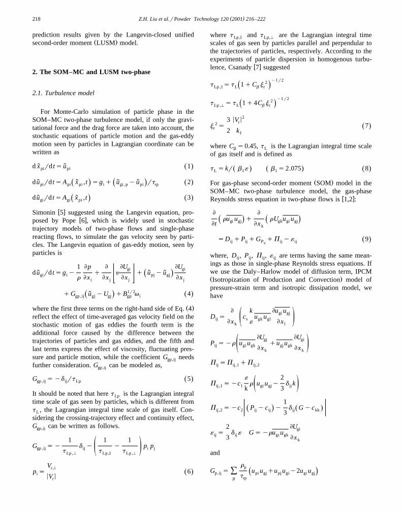
Fig. 1. Geometrical configuration of the chamber.

is the gas Reynolds stress productionrdestruction due toparticles drag force. The transport equation of dissipationrate of gas turbulent kinetic energy is:

E Er´ q rU ´Ž . Ž .gk

Et Ex k

E k E´ ´s c u u q c GqG yc r´Ž .´ gk gl ´1 p ´ 2ž /Ex ´ Ex kk l

10Ž .

where

rpG s u u yu uŽ .Ýp pi gi gi gi

trpp

For the Langevin-closed unified second-order momentŽ .model LUSM , beside the gas-phase equations, the fol-

lowing particle-phase equations are adoptedParticle Continuity

En En Up p pkq 11Ž .

Et Ex k

Particle Momentum

En U En U U np pi p pk pi pq sn g q U qV yUŽ .p i gi di pi

Et Ex tk rp

En up pk py 12Ž .

Ex k

Particle Reynolds Stress

En u u En U u up pi pj p pk pi pjq

Et Ex k

En u u u EU EUp pk pi pj pi pjsy yn u u q up pk pj pk pž /Ex Ex Exk k k

npq u u qu u y2u 13Ž .Ž .gi pj gj pi pi p

trp

Gas–Particle Fluctuation Velocity Correlation

En u u En U u up gi pj p pk gi pjq

Et Ex k

En u u u EU EUp pk gi pj pj gisy yn u u qu up pk gi gk pjž /Ex Ex Exk k k

EV ndi pyn u u y u u yu uŽ .p gk pj gi pj gi gj

Ex tk rp

qn G u 14Ž .p gp ,im gm p

Particle Drift Velocity

En V En U V En u u yu up di p pk di p pk gi gk giq sy yu ugk gi

Et Ex Exk k

EUgiyn V qn G 15Ž .p dk p gp ,ij d

Ex k

where

Eupi pu u u fyG ,pk pi pj p ,km

Em

Eugi pu u u fyG ,pk gi pj pg ,km

Em

5G s t u u q ,p ,ij rp pi pj pg ,i9

G s0.22t upg ,ij E gi p

3. Simulation of swirling gas–particle

3.1. Flows

The SOM–MC and LUSM models were used to simu-late swirling gas–particle flows with a swirl number of

w x0.47, measured by PDPA 15 . The geometrical configura-tion and sizes of the chamber are shown in Fig. 1. Thelength of the chamber is 950 mm. The particle phase isglass beads with mean diameter of 30 mm and material

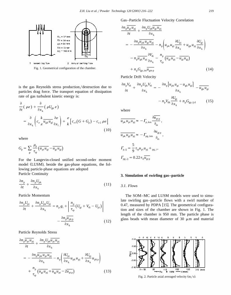
Ž .Fig. 2. Particle axial averaged velocity mrs .

( )Z.H. Liu et al.rPowder Technology 120 2001 216–222220

Ž .Fig. 3. Particle tangential averaged velocity mrs .

density of 2.15=103 kgrm3. The inlet flow parametersare central mass flow rate 9.9 grs annular mass flow rate38.5 grs and particle mass loading 0.034. A staggered-gridsystem with 32=20 grid nodes are adopted.

In specifying the boundary conditions of gas phase theinlet velocities and normal components of Reynolds stressesare given by experiments the shear stresses are given bythe eddy-viscosity assumption. The fully developed flowcondition is taken at the exit. The above-specified inlet andexit conditions are made by most of the numerical model-ers using second-order moment models. Although one cansimply assume a uniform inlet-velocity distribution andisotropic normal stresses at the inlet, in a pipe flow theinlet velocity is non-uniform and the normal stresses areanisotropic. The fully developed flow condition at the exitis an approximate one, which may cause the under-predict-ion of the recirculation zones since in fact within a cham-ber of LrDs5 the flow cannot reach fully developed.However, for an elliptical problem, we have to give theexit condition, which is difficult to be specified in ad-vance. At the walls, no-slip condition is used for gasvelocity and the gas Reynolds stress components as well asgas velocities are determined via production term, includ-ing the effect of wall functions for near-wall grid nodes. Atthe axis, the symmetrical condition is adopted. For bound-ary conditions of particle-phase at the inlet, the particlevelocities are assumed to have a Gaussian distribution,with averaged velocities and normal stresses equal to thosemeasured. The particle-wall collision is taken as elasticone with no energy loses. At the axis the symmetricalcondition is adopted.

The gas-phase equations in the SOM model and two-phase equations in the LUSM model are solved using an

w xextended version of SIMPLEC algorithm 16 . In theMonte-Carlo simulation of particle phase, the stochastic

Ž Ž . Ž . Ž .equations of particle-phase, Eqs. 1 , 2 , and 4 , aresolved using a second-order Runge–Kutta method. Five

Ž .Fig. 4. Particle axial fluctuation velocity mrs .

Ž .Fig. 5. Particle tangential fluctuation velocity mrs .

Ž .million nearly 10,000 in each cell computational particlesare distributed uniformly throughout the computationaldomain. Each particle has different values of its spatial

Ž . Ž .position X , velocity U and the gas velocity seen by itpŽ .U . These values of particles will evolve according tof,p

Ž . Ž . Ž .the stochastic equations, Eqs. 1 , 2 and 4 , which aresolved by integration with a certain time-step, until asteady-state solution is reached. The time-step is taken as0.2 ms. Particle calculation is conducted with five time-stepafter five-time gas-phase iterations. At each time-step, theparticle averaged velocities, particle Reynolds stresses andthe gas–particle fluctuation velocity correlations in eachcell are determined by an ensemble averaging procedure,according to the instantaneous behavior of marking parti-cles in that cell. Then, the particle source term is added tothe gas-phase equations and next iteration is started, untilthe summation of residual mass source of the gas flowfield is less than 0.001.

The computer codes SOM–MC and LUSM are writtenin standard FORTRAN-77 language. Running a case on anSGI-O2 workstation or a Pentium-II-300 PC computerneeds about 560 min for the SOM–MC code, and needsabout 56 min for the LUSM code.

4. Results and discussion

Because the case studied is dilute gas–particle flows,the effect of particle phase on the gas flow field isnegligible, the simulation results for the gas phase are notpresented here. Figs. 2–5 give the predicted result usingthe SOM–MC model and the LUSM model in comparison

w xwith the PDPA measurements 15 . It can be seen that bothtwo models can well predict the time-averaged particleaxial and tangential velocities in good agreement with the

Ž .Fig. 6. Gas and particle axial fluctuation velocities mrs, Exp. .

( )Z.H. Liu et al.rPowder Technology 120 2001 216–222 221

Ž .Fig. 7. Gas and particle tangential fluctuation velocities mrs, Exp. .

Ž .measurement results Figs. 2 and 3 , and there is onlyslight difference between these two models. However, theSOM–MC model gives the predicted particle axial aver-aged velocity and its fluctuation in better agreement withexperiments than the LUSM model in the near inlet region,at xs52 mm. The SOM–MC model can predict thereverse flow in that region, which cannot be predicted bythe LUSM model. Since there is no difference in theclosure methods between these two models, it can beconsidered that the difference is caused only by numericalmethods. The Monte-Carlo method or the Lagrangianmethod is free of numerical-diffusion. As for the particle

Ž .axial and tangential fluctuation velocities Figs. 4 and 5 ,they are significantly under-predicted, no matter whetherthe Eulerian–Lagrangian SOM–MC model or the Eule-rian–Eulerian LUSM model is used. The difference be-tween the two models is once again very small. Actually

w xall of the USM models developed in 17,18 with differentclosure methods other than the Langevin equation givealmost the same results as those obtained here. Figs. 6–9give the comparison of predicted gas and particle fluctua-tion velocities using the SOM–MC model with the experi-mental results. Clearly, the model predictions give theright tendency in the relationship between gas and particlefluctuation velocities. The predicted particle axial fluctua-tion velocity exceeds the gas one in the reverse-flow zone,as clearly seen in the section xs52 mm, and the pre-dicted particle tangential fluctuation velocity is smallerthan the gas one everywhere. This predicted tendency is inagreement with that observed in experiments.

The discrepancy between the predicted and measuredfluctuation velocities needs to be further analyzed. Up tonow, all of particle-phase turbulence models, includingEulerian and Lagrangian models, unified second-order mo-

Ž .Fig. 8. Gas and particle axial fluctuation velocities mrs, SOM–MC .

Ž .Fig. 9. Gas and particle tangential fluctuation velocities mrs, SOM–MC .

ment models with different closure methods, obviouslygive the same averaged flow field and all models underpre-

w xdict the two-phase fluctuation velocities. Fu 19 and Zhouw xand Xu 20 simulated strongly swirling single-phase flows

with a swirl number of ss0.53, using the second-ordermoment model, and found that the SOM model can wellpredict the single-phase turbulence. So, the discrepancymay be caused by the particle–wall and particle–particlecollision in the near-wall region of high particle concentra-tion, which should increase the particle turbulence. On theother hand, the gas-phase turbulence model in two-phaseflows needs to be revisited. The turbulence dissipation ofgas phase in case of two-phase flows should be determinednot only by the Kolmogorov mechanism, but also by theeffect of particles. Right now these problems are underinvestigation.

5. Conclusions

Ž .1 Both Eulerian–Lagrangian SOM–MC model andEulerian–Eulerian LUSM model closed by the sameLangevin equation, or USM models using other closuremethods different from Langevin equation, give almost thesame results in predicting swirling gas–particle flows.

Ž .2 The merits of the SOM–MC model is free ofnumerical diffusion, so it gives better prediction results inthe near-inlet region. The drawback of this model is that itneeds much more computation time than the LUSM modeland other USM models.

Ž .3 All of E–L and E–E models underpredict thetwo-phase Reynolds stresses or fluctuation velocities inswirling flows. To further improve these models, the parti-cle–particle collision in the near-wall region, the particle–wall interaction and the effect of particles on gas turbu-lence dissipation should be taken into account.

Acknowledgements

This study was sponsored by the Special funds for theMajor State Basic Research, PRC. The authors would liketo thank Dr. Chen T., who provided the basic USMcomputer code, and Prof. Chen Y.L., who provided thebasic Monte-Carlo computer code.

( )Z.H. Liu et al.rPowder Technology 120 2001 216–222222

References

w x1 L.X. Zhou, Theory and Numerical Modeling of Turbulent Gas–Par-ticle Flows and Combustion, Science Press, Beijing and CRC Press,Florida, 1993.

w x2 L.X. Zhou, C.M. Liao, T. Chen, A unified second-order momenttwo-phase turbulence model for simulating gas–particle flows,

Ž .ASME FED 185 1994 307–313.w x3 I.V. Derevich, L.I. Zaichik, The equation for the probability density

of the particle velocity and temperature in a turbulent flow simulatedŽ . Ž .by the Gauss Stochastic field, Prikl. Mat. Mekh 54 5 1990 767.

w x4 M.W. Reeks, On a kinetic equation for the transport of particles inŽ .turbulent flows, Phys. Fluids A 3 1991 446–456.

w x5 O. Simonin, Continuum modeling of dispersed turbulent two-phaseflows,VKI Lectures: Combustion in Two-phase Flows, Jan 29–Feb.2, 1996.

w x6 S.B. Pope, PDF methods for turbulent reactive flows, Prog. EnergyŽ .Combust. Sci. 11 1985 119–192.

w x7 G.T. Csanady, Turbulent diffusion of heavy particle in the atmo-Ž .sphere, J. Atmos. Sci. 20 1963 201–208.

w x8 L.X. Zhou, Y. Xu, A Second-order Moment Particle TurbulenceClosure Based on Lagrangian Analysis, ASME-FEDSM 2000, Paper11153, Boston, 2000.

w x9 L.P. Wang, D.E. Stock, Dispersion of heavy particles by turbulentŽ .motion, J. Atmos. Sci. 50 1993 1897–1913.

w x10 X.Y. Huang, D.E. Stock, Using the Monte-Carlo process to simulatetwo-dimensional heavy particle dispersion in a uniformly shearedturbulent flow, Numerical Methods in Multiphase Flows, ASME

Ž .FED 185 1994 243–249.w x11 V. Mehrotra, G.D. Silcox, P.J. Smith, Numerical simulation of

turbulent particle dispersion using a Monte Carlo approach, Proc. ofFEDSM’98, Washington, DC, 1998.

w x12 L.X. Zhou, Y. Li, A new statistical theory and a k-´-PDF model forsimulating turbulent gas–particle flows, Inter. Symp. on Math.

ŽModeling of Turb. Flows, Tokyo, 1995, pp. 399–404 Tsinghua.Science and Technology, v. 2, n. 2, 628–632, 1997 .

w x13 L.X. Zhou, C.G. Zheng, Z.H. Liu, The joint PDF transport equationof combusting particle phase in turbulent reacting gas–particle flows,ASME 8th Int. Symp. on Gas–Particle Flows, San Francisco, 1999.

w x14 J. Pozorski, J.P. Minier, On the Lagrangian turbulent dispersionmodels based on the Langevin equation, Int. J. Multiphase Flow 24Ž .1998 913–945.

w x15 M. Sommerfeld, H.H. Qiu, Detailed measurements in a swirlingparticulate two-phase flow by a phase-Doppler anemometer, Int. J.

Ž .Heat Fluid Flow 12 1991 15–32.w x16 S.V. Patankar, Numerical heat transfer and fluid flow, Hemisphere

Ž .1980 .w x17 L.X. Zhou, Y. Li, T. Chen, Comparison between different two-phase

turbulence models for simulating swirling gas–particle flows, Proc.ASME-FED 1998 Summer Meeting v. 245, Washington, DC, 1998.

w x18 Y. Yu, L.X. Zhou, C.G. Zheng, Z.H. Liu, Comparison betweentime-averaged and mass-weighed averaged unified second-order mo-ment two-phase turbulence models using different closures, to bepublished.

w x19 S. Fu, Modeling of the strongly swirling flows with second-momentŽ .closure, in: Z.S. Zhang, Y. Miyake Eds. , The Recent Develop-

Žments In Turbulence Research Proc. of SINO-JAPAN Workshop of.Turbulent Flows , Int. Academic Publishers, Beijing, 1994, pp.

22–41.w x20 L.X. Zhou, Y. Xu, Simulation of swirling gas–particle flows using

an improved second-order moment two-phase turbulence model, tobe published in Powder Technology.