a second order discontinuous galerkin fast sweeping method...

A Second Order Discontinuous Galerkin Fast Sweeping Method

for Eikonal Equations

Fengyan Li1, Chi-Wang Shu2, Yong-Tao Zhang3, and Hongkai Zhao4

ABSTRACT

In this paper, we construct a second order fast sweeping method with a discontinuous Galerkin

(DG) local solver for computing viscosity solutions of a class of static Hamilton-Jacobi equations,

namely the Eikonal equations. Our piecewise linear DG local solver is built on a DG method

developed recently [Y. Cheng and C.-W. Shu, A discontinuous Galerkin finite element method

for directly solving the Hamilton-Jacobi equations, Journal of Computational Physics, 223 (2007),

398-415] for the time-dependent Hamilton-Jacobi equations. The causality property of Eikonal

equations is incorporated into the design of this solver. The resulting local nonlinear system in the

Gauss-Seidel iterations is a simple quadratic system and can be solved explicitly. The compactness

of the DG method and the fast sweeping strategy lead to fast convergence of the new scheme for

Eikonal equations. Extensive numerical examples verify efficiency, convergence and second order

accuracy of the proposed method.

Key Words: fast sweeping methods, discontinuous Galerkin finite element methods, second

order accuracy, static Hamilton-Jacobi equations, Eikonal equations

1Department of Mathematical Sciences, Rensselaer Polytechnic Institute, Troy, NY 12180, USA. E-mail:

[email protected]. Research supported by NSF grant DMS-0652481.2Division of Applied Mathematics, Brown University, Providence, RI 02912, USA. E-mail: [email protected].

Research supported by NSF grant DMS-0510345.3Department of Mathematics, University of Notre Dame, Notre Dame, IN 46556-4618, USA. E-mail:

[email protected] of Mathematics, University of California, Irvine, CA 92697-3875, USA. E-mail: [email protected].

Research partially supported by NSF grant DMS-0513073, ONR grant N00014-02-1-0090 and DARPA grant N00014-

02-1-0603.

1

1 Introduction

In this paper, we develop a second order fast sweeping method for numerically solving an important

class of static Hamilton-Jacobi (H-J) equations, namely the Eikonal equations

|∇φ(x)| = f(x), x ∈ Ω\Γ, (1.1)

φ(x) = g(x), x ∈ Γ ⊂ Ω, (1.2)

where Ω belongs to R2 with Γ as its subset, e.g., the boundary, and 0 < c < f(x) < C < ∞

for some positive c, C and f(x) and g(x) are Lipschitz continuous. Such equations appear in

many applications, such as optimal control, differential games, level set method, image processing,

computer vision, and geometric optics.

Since the boundary value problems (1.1)-(1.2) are nonlinear first order partial differential equa-

tions, we may apply the classical method of characteristics to solve these equations in phase space;

namely, consider the gradient components as independent variables and solve ODE systems to fol-

low the propagation of characteristics. Although the characteristics may never intersect in phase

space, their projection into physical space may intersect so that the solution in physical space is

not uniquely defined at these intersections. By mimicking the entropy condition for hyperbolic

conservation laws to single out a physically relevant solution, Crandall and Lions [16] introduced

the concept of viscosity solutions for H-J equations so that a unique global weak solution can be

defined for such first order nonlinear equations. Moreover, monotone finite difference schemes are

developed to compute such viscosity solutions stably.

There are mainly two classes of numerical methods for solving static H-J equations. The first

class of numerical methods is based on reformulating the equations into suitable time-dependent

problems. Osher [32] provides a natural link between static and time-dependent H-J equations

by using the level-set idea and thus raising the problem one-dimensional higher. In the control

framework, a semi-Lagrangian scheme is obtained for H-J equations by discretizing in time the

dynamic programming principle [19, 20]. Another approach to obtaining a “time” dependent H-

J equation from the static H-J equation is using the so called paraxial formulation in which a

preferred spatial direction is assumed in the characteristic propagation [21, 17, 29, 36, 37]. High

order numerical schemes are well developed for the time dependent H-J equation on structured and

unstructured meshes [34, 25, 51, 24, 33, 7, 26, 31, 35, 1, 3, 4, 6, 8]; see a recent review on high

order numerical methods for time dependent H-J equations by Shu [46]. Due to the finite speed of

propagation and the CFL condition for the discrete time step size, the number of time steps has to

2

be of the same order as that for one of the spatial dimensions so that the solution converges in the

entire domain.

The other class of numerical methods for static H-J equations is to treat the problem as a

stationary boundary value problem: discretize the problem into a system of nonlinear equations

and design an efficient numerical algorithm to solve the system. Among such methods are the fast

marching method and the fast sweeping method. The fast marching method [48, 43, 22, 44, 45]

is based on the Dijkstra’s algorithm [18]. The solution is updated by following the causality in

a sequential way; i.e., the solution is updated pointwise in the order that the solution is strictly

increasing (decreasing); hence two essential ingredients are needed in the algorithm: an upwind

difference scheme and a heap-sort algorithm. The resulting complexity of the fast marching method

is of order O(N logN) for N grid points, where the logN factor comes from the heap-sort algorithm.

Recently, an O(N) implementation of the fast marching algorithm for solving Eikonal equations is

developed in [50]. The improvement is achieved by introducing the untidy priority queue, obtained

via a quantization of the priorities in the marching computation. However, the numerical solution

obtained by this algorithm is not an exact solution to the discrete system due to quantization. The

extra error introduced must be controlled to be at the same order as the numerical error of the

discretization scheme. It is shown in [40] that the complexity of this algorithm is O(fmax/fminN)

in order to achieve an accuracy that is independent of the variation of f(x). In the fast sweeping

method [5, 55, 47, 54, 27, 28, 53, 38, 39, 52], Gauss-Seidel iterations with alternating orderings is

combined with upwind finite differences. In contrast to the fast marching method, the fast sweeping

method follows the causality along characteristics in a parallel way; i.e., all characteristics are

divided into a finite number of groups according to their directions and each Gauss-Seidel iteration

with a specific sweeping ordering covers a group of characteristics simultaneously; no heap-sort is

needed. The fast sweeping method is optimal in the sense that a finite number of iterations is

needed [54], so that the complexity of the algorithm is O(N) for a total of N grid points, although

the constant in the complexity depends on the equation. The algorithm is extremely simple to

implement. Moreover, the iterative framework is more flexible for general equations and high order

methods.

The high order finite difference type fast sweeping method developed in [53] provides a quite

general framework, and it is easy to incorporate any order of accuracy and any type of numerical

Hamiltonian into the framework. Much faster convergence speed than that by the time-marching

approach can be achieved. Due to the wide stencil of the high order finite difference approximation

3

to the derivatives, some downwind information is used and the computational complexity of high

order finite difference type fast sweeping methods is slightly more than linear.

Discontinuous Galerkin (DG) methods, on the other hand, can achieve high order accuracy by

using very compact stencil. In this paper, we develop a second order fast sweeping method based

on a DG local solver for an important class of static H-J equations, namely the Eikonal equations.

A very fast convergence speed is observed in the numerical experiments.

The DG method is a class of finite element methods, using discontinuous piecewise polynomials

as approximations for solutions and test functions. The main difference between the DG method

and the finite difference or finite volume method is that the former stores and solves for a complete

polynomial in each cell, while the latter stores and solves for only one piece of information (the

point value for the finite difference scheme and the cell average for the finite volume scheme) in

each cell, and it must resort to a reconstruction or interpolation using a wide stencil of neighboring

cells in order to achieve higher order accuracy. The DG method was first designed as a method

for solving hyperbolic conservation laws containing only first order spatial derivatives, e.g. Reed

and Hill [42] for solving linear equations, and Cockburn et al. [12, 11, 10, 13] for solving nonlinear

equations. In recent years the DG method has also been extended to solve many other nonlinear

PDEs such as the convection diffusion equations [14], KdV type dispersive wave equations [49], etc.

Even though the approximation spaces of the DG method consist of discontinuous functions, the

DG method can also be used to approximate continuous and even smooth solutions like in elliptic

equations. The key point is that discontinuities at the cell boundary are automatically controlled

to be consistent with the approximation error inside the cell for a well designed DG method. We

refer to [15, 2] for more details about DG methods.

There are mainly two types of DG methods for solving H-J equations. One was originally

proposed in [24, 23] which is based on the observation that the gradient of the solution φ of the H-J

equations satisfies a hyperbolic system. The DG method combined with a least squares procedure,

is then applied to solve the system to get the gradient of φ. The missing constant in φ is further

recovered through the original equation. This method is later reinterpreted and simplified in [30] by

using the piecewise curl-free solution space in DG method. In another recent work on DG method

for H-J equation [9], the solution φ is solved directly. This method is more desirable in the sense

that the derived hyperbolic system for ∇φ in [24, 30] involves more unknown functions than the

original scalar H-J equation which is solved directly in [9]. Moreover the solutions of H-J equations

generally are smoother than those of the conservations laws.

4

Based on the DG discretization in [9], in this paper, we develop a second order fast sweeping

method for solving Eikonal equations by incorporating the causality property of these equations

into the DG local solver. The resulting local nonlinear system in the Gauss-Seidel iterations is a

simple quadratic system and can be solved explicitly. The compactness of the DG method and the

fast sweeping strategy lead to a very fast convergence of the new scheme for Eikonal equations. The

rest of the paper is organized as follows. The algorithm is developed in Section 2, and numerical

examples are given in Section 3 to demonstrate the accuracy and the fast convergence of the method.

Concluding remarks are given in Section 4.

2 Numerical Formulation

Let q = ∇xφ and H(q) = |q| − f(x), q ∈ R2, then the characteristic equations of the Eikonal

equation (1.1)-(1.2) are

x =∇qH =q

f(2.1)

q =∇xf (2.2)

φ =∇xφ · x = q · ∇qH = f(x) > 0 (2.3)

One can see that φ is increasing along the characteristics, which is an important component in the

design of the efficient methods for solving (1.1)-(1.2).

One of the key ingredients in designing a fast sweeping method is to design a local solver, which

expresses the value at the standing mesh point in terms of its neighboring values, and (1) it is

consistent with the causality of the PDE and is able to deal with possible discontinuities in the

derivatives, and (2) the resulting nonlinear equation can be solved efficiently during the Gauss-

Seidel iterations. The second order local solver developed in this paper is based on the second type

discontinuous Galerkin method [9] reviewed in the introduction. The main idea will be presented

for the cases with rectangular meshes.

We start with a partition of Ω = ∪1≤i≤I,1≤j≤JIij where Iij = Ii × Jj and Ii = [xi−1/2, xi+1/2],

Jj = [yj−1/2, yj+1/2]. The centers of Ii, Jj are denoted by xi = 12(xi−1/2+xi+1/2) and yj = 1

2(yj−1/2+

yj+1/2), and the lengths of Ii, Jj are denoted by ∆xi = xi+1/2 − xi−1/2 and ∆yj = yj+1/2 − yj−1/2.

In this paper, we take ∆xi = ∆yj = h for simplicity of the presentation. We further define the

piecewise linear approximation space as

V 1h = v : v|Iij

∈ P 1(Iij),∀i, j

5

where P 1(Iij) is the set of linear polynomials on Iij . Following the idea of the method developed

in [9], a numerical scheme for (1.1) can be formulated as follows: find φh ∈ V 1h , such that

∫

Iij

|∇φh|wh(x, y)dxdy + αr,ij

∫

Jj

[φh](xi+ 1

2

, y)wh(x−i+ 1

2

, y)dy + αl,ij

∫

Jj

[φh](xi− 1

2

, y)wh(x+i− 1

2

, y)dy

+ αt,ij

∫

Ii

[φh](x, yj+ 1

2

)wh(x, y−j+ 1

2

)dx+ αb,ij

∫

Ii

[φh](x, yj− 1

2

)wh(x, y+j− 1

2

)dx

=

∫

Iij

f(x, y)wh(x, y)dxdy, ∀ i, j, ∀ wh ∈ V 1h (2.4)

Let us now explain the notations in (2.4). For the piecewise smooth function φh ∈ V 1h , [φh] denotes

the jump of φh across the cell interface which is defined horizontally by [φh](xi+ 1

2

, ·) = φh(x+i+ 1

2

, ·)−φh(x−

i+ 1

2

, ·), ∀ i and vertically by [φh](·, yj+ 1

2

) = φh(·, y+j+ 1

2

) − φh(·, y−j+ 1

2

), ∀ j. Here φh(x+i+ 1

2

, y) =

φh|Ii+1,j(xi+ 1

2

, y), φh(x−i+ 1

2

, y) = φh|Iij(xi+ 1

2

, y) for y ∈ Jj , and φh(x, y+j+ 1

2

) = φh|Ii,j+1(x, yj+ 1

2

),

φh(x, y−j+ 1

2

) = φh|Iij(x, yj+ 1

2

) for x ∈ Ii. αr,ij, αl,ij , αt,ij , αb,ij are constants which only depend on

the numerical solutions in the neighboring cells of Iij , and they are one of the important components

of the local solver. By properly choosing these functions, we expect that the formulation (2.4) is not

only accurate and stable, but also enforces the causality of the Eikonal equation therefore making

it possible to design an efficient fast sweeping algorithm for solving (1.1)-(1.2).

The piecewise linear approximation φh|Iijcan be written as φh|Iij

= φij + uijXi + vijYj , where

φij , uij, vij are the unknowns, and Xi = x−xi

h , Yj =y−yj

h . Note that φij is the cell average of φh

over Iij.

With the consideration of the causality of the Eikonal equation (1.1)-(1.2), we choose the con-

stants αr,ij, αl,ij, αt,ij, αb,ij in the formulation (2.4) as following:

αl,ij =

max(0, ui−1,j/(hfi−1,j)) when φi−1,j ≤ φi+1,j ;0 when φi−1,j > φi+1,j ,

(2.5)

αr,ij =

0 when φi−1,j ≤ φi+1,j;min(0, ui+1,j/(hfi+1,j)) when φi−1,j > φi+1,j,

(2.6)

αb,ij =

max(0, vi,j−1/(hfi,j−1)) when φi,j−1 ≤ φi,j+1;0 when φi,j−1 > φi,j+1,

(2.7)

αt,ij =

0 when φi,j−1 ≤ φi,j+1;min(0, vi,j+1/(hfi,j+1)) when φi,j−1 > φi,j+1,

(2.8)

where fi,j = f(xi, yj). If we denote H1 = ∂H∂φx

and H2 = ∂H∂φy

, one would notice that the constants

αr,ij, αl,ij , αt,ij , αb,ij are approximations of H1(∇φh) and H2(∇φh) in the four neighboring cells

of Iij , with min and max operations to enforce the consistency of the causality. For instance

when φi−1,j ≤ φi+1,j and φi,j−1 ≤ φi,j+1, that is when the information is propagating from the

bottom-left to the top-right in the neighborhood of the cell Iij , we expect the causality consistency

6

that H1(∇φh)|Ii−1,j≈ ui−1,j/(hfi−1,j) > 0, H2(∇φh)|Ii,j−1

≈ vi,j−1/(hfi,j−1) > 0 for the current

numerical solution in neighboring cells Ii−1,j and Ii,j−1. So if this holds, αl,ij and αb,ij will be

non-zeros and the scheme (2.4) becomes∫

Iij

|∇φh|wh(x, y)dxdy + αl,ij

∫

Jj

[φh](xi− 1

2

, y)wh(x+i− 1

2

, y)dy + αb,ij

∫

Ii

[φh](x, yj− 1

2

)wh(x, y+j− 1

2

)dx

=

∫

Iij

f(x, y)wh(x, y)dxdy, ∀ i, j, ∀ wh ∈ V 1h (2.9)

In other words, the method reflects the fact that the solution is increasing along the characteristics.

Remark 2.1 The choices for αl,ij, αr,ij, αb,ij and αt,ij in this paper are different from those used

in [9]. For any given (i, j), these functions do not depend on φh|Iij, and this is crucial in order to

get a simple local solver for (2.4) which forms a building block of the fast convergence algorithm,

see Section 2.1 and Section 3. On the other hand, it is indicated in [9] (on page 400) that as long as

αl,ij is within O(h) perturbation of H1(∇φh(xi−1/2, yj)) (similar argument goes to αr,ij, αb,ij and

αt,ij), the accuracy developed in [9] is guaranteed by truncation error analysis and this is confirmed

by numerical tests. Our choice of αl,ij, αr,ij, αb,ij and αt,ij satisfies such conditions therefore will

maintain the accuracy results in [9].

If Iij ∩ (∂Ω\Γ) is not empty for some (i, j), we modify (2.5)-(2.8) in this cell to carry out the

outflow boundary condition. For instance in the cell Iij where xi+ 1

2

is aligned with the domain

boundary and Iij ∩ Γ is empty, we take αr,ij = 0. Similar adjustment is made to αl,ij, αt,ij , αb,ij .

For any given (i, j), by taking wh = 1, Xi, Yj on Iij and wh = 0 elsewhere, the DG formulation

(2.4) can be converted from the integral form to the following nonlinear algebraic system:

√

u2ij + v2

ij + γijφij + βijuij + λijvij = R1,ij (2.10)

12βij φij + ζijuij = R2,ij (2.11)

12λij φij + ηijvij = R3,ij (2.12)

where

βij = −1

2(αr,ij + αl,ij), λij = −1

2(αt,ij + αb,ij)

γij = αl,ij − αr,ij + αb,ij − αt,ij

ζij = −3αr,ij + 3αl,ij − αt,ij + αb,ij

ηij = −3αt,ij + 3αb,ij − αr,ij + αl,ij

7

and

R1,ij =1

h

∫

Iij

f(x, y)dxdy − αr,ij(φi+1,j −1

2ui+1,j) + αl,ij(φi−1,j +

1

2ui−1,j)

− αt,ij(φi,j+1 − 1

2vi,j+1) + αb,ij(φi,j−1 +

1

2vi,j−1)

R2,ij =12

h

∫

Iij

f(x, y)Xidxdy − 6αr,ij(φi+1,j −1

2ui+1,j) − 6αl,ij(φi−1,j +

1

2ui−1,j) − αt,ijui,j+1 + αb,ijui,j−1

R3,ij =12

h

∫

Iij

f(x, y)Yjdxdy − 6αt,ij(φi,j+1 − 1

2vi,j+1) − 6αb,ij(φi,j−1 +

1

2vi,j−1) − αr,ijvi+1,j + αl,ijvi−1,j

To solve the coupled nonlinear system (2.10)-(2.12) with 1 ≤ i ≤ I, 1 ≤ j ≤ J efficiently, we are

going to propose a fast sweeping method which uses block Gauss-Seidel iterations with alternating

directions of sweepings. Based on the basic steps of the fast sweeping methods in [47, 54], we first

need to define a local solver to compute φh in Iij based on the DG discretization (2.10)-(2.12),

provided that the solution in the remaining region is known.

2.1 DG local solver

Note that βij, λij , γij , ζij , ηij in (2.10)-(2.12) are functions of αr,ij, αl,ij, αt,ij, and αb,ij defined in

(2.5)-(2.8), which are independent of φh|Iij. In addition, R1,ij , R2,ij and R3,ij in (2.10)-(2.12) are

independent of φh|Iij. These indicate that the system of equations (2.10)-(2.12) provides a local

representation of (φij , uij , vij) in terms of the unknown solution φh in the neighboring cells and the

source data. Moreover, (2.10)-(2.12) is quadratic with respect to (φij , uij , vij).

Given (i, j), let φnewh |Iij

= φnewij + unew

ij Xi + vnewij Yj denote the candidate for the update of the

numerical solution φh in Iij and φh|Ikl= φkl + uklXi + vklYj denote the current numerical solution

in any (k, l)-th cell, then we compute φnewh according to the following formula

√

(unewij )2 + (vnew

ij )2 + γijφnewij + βiju

newij + λijv

newij = R1,ij, (2.13)

12βij φnewij + ζiju

newij = R2,ij, (2.14)

12λijφnewij + ηijv

newij = R3,ij. (2.15)

Note that βij, λij , γij , ζij , ηij , R1,ij , R2,ij , R3,ij do not depend on the numerical solution in Iij , hence

(2.13)-(2.15) defines a quadratic system for (φnewij , unew

ij , vnewij ) which can be solved explicitly. We

can also show that the parameters γij , ζij , ηij are either all zero or all positive. Since the system

(2.13)-(2.15) in principle can have none or two sets of solutions of (φnewij , unew

ij , vnewij ), we take

the following strategy to decide when to reject or to accept the candidates of (φnewij , unew

ij , vnewij )

computed from (2.13)-(2.15), based on the causality of the Eikonal equation:

8

1. When γij , ζij , ηij are all zero, we will not update the solution in this cell;

2. When γij , ζij , ηij are all positive, if we get from (2.13)-(2.15)

• two sets of real solutions (φnewij , unew

ij , vnewij ): then update φh|Iij

with φnewh |Iij

if the

following conditions are satisfied:

φnewij ≥ φi−1,j and unew

ij ≥ 0, if αl,ij > 0

φnewij ≥ φi+1,j and unew

ij ≤ 0, if αr,ij < 0

φnewij ≥ φi,j−1 and vnew

ij ≥ 0, if αb,ij > 0

φnewij ≥ φi,j+1 and vnew

ij ≤ 0, if αt,ij < 0

(2.16)

If both sets of the solutions satisfy the above conditions, choose the one with the smaller

value of φnewij ;

• two sets of complex solutions: we will not update the solution in this cell.

Remark 2.2 The strategy regarding accepting or rejecting the candidate solutions in (2.16) is to

ensure the consistency of the causality. For example, if we follow the discussion after the definition

of αl,ij to αt,ij in (2.5)-(2.8) when the information is propagating from the bottom-left to the top-

right in the neighborhood of the cell Iij, we expect αl,ij > 0 and αb,ij > 0, therefore we accept

the candidate solution (φnewij , unew

ij , vnewij ) which is consistent with the causality: φnew

ij ≥ φi−1,j,

φnewij ≥ φi,j−1 as well as unew

ij ≥ 0, vnewij ≥ 0. That is, along the characteristic the solution is

nondecreasing. Note that comparing average values in cells does not necessarily give the correct

information of the characteristics or monotonicity of the solution. That explains why oscillations

can occur (see Example 7 in Section 3) if the derivative criterion is not used, i.e., the average is

monotone even if the solution is not. However, the sign of derivatives become subtle near local

extrema or shocks. So in (2.16) we use both the cell average and the derivatives of the solution to

decide the acceptance or the rejection of a candidate for the solution update to ensure the causality

consistency.

2.2 Hybrid DG local solver

With the local solver defined in the previous section as the building block, the numerical experiments

show that the straightforward application of the fast sweeping method as in [47, 54] based on the

DG discretization (2.4) may not produce satisfactory results all the time. There are two issues

that we need to pay more attention. The first is the initial data. In general iterative methods for

9

nonlinear problems need a good initial guess for convergence, in particular when they are based on

high order discretizations. On the other hand, the fast sweeping method based on the first order

Godunov scheme has been shown monotone, convergent and efficient for any initial data that are

super-solution (or sub-solution) of the true viscosity solution [54]. So we use the first order scheme

to provide a good initial guess for our high order method just as in [53], see Section 2.3 for the

complete description.

The second issue is that we enforce a quite strong causality condition (2.16) when we update

the value in a cell using the local DG solver. Near shocks, where characteristics intersect, or near

points where φx or φy are close to zero, causality issue becomes more subtle. The local DG solver

may not be able to provide a solution satisfying (2.16). Hence in those cells where the second order

local DG solver can not provide a solution we switch back to a first order finite difference type

Godunov scheme. The hope is that more accurate information propagated through the DG solver

will be felt at all points.

However, those conditions in (2.16) will enforce propagation of information in the right direction

and this will significantly reduce the number of iterations of our final algorithm in Section 2.4. For

example, such conditions were not used in [53] and more iterations are needed in general.

One concern for hybridizing the two local solvers is a possible reduction of the accuracy. In

practice the first order local solver is only used rarely as explained above. This phenomenon is

observed in our numerical examples. Here we classify the convergence of our method into three

cases.

C1: The first order finite difference type local solver is never used;

C2: The first order finite difference type local solver is used before the iterations converge. By

the time the iterations converge, the first order local solver is not used.

C3: The first order finite difference type local solver is used in the whole process of the com-

putation. By the time the iterations converge, the first order local solver is used in certain

cells and the solution is not further updated if the iterations continue. The ratio between

the number of the cells in which the first order local solver is used and the number of the

total cells is decreasing when h decreases, and the numerical evidence shows that this ratio

is about O(h).

Remark 2.3 Numerical examples show that in the case C3 described above, the first order local

solver is used in O(h) percentage of the total number of cells which are in the neighborhood of the

10

shock location, i.e., where characteristics intersect, and hence it does not pollute solutions in other

region. Therefore the method still achieves second order accuracy in the L1 norm.

The hybrid local solver is defined as follows: given (i, j)

(1) When the DG local solver defined in the previous section provides an update in Iij, the update

is accepted;

(2) When the DG local solver defined in the previous section provides no update in Iij , the

following finite difference based local solver is used instead: let

a = min(φi−1,j, φi+1,j), b = min(φi,j−1, φi,j+1), fi,j = f(xi, yj),

we then update the solution in the cell Iij as the following:

• If |a− b| ≥ fi,jh, then

φnewi,j = min(a, b) + fi,jh

and

unewij = φnew

ij − φi−1,j, vnewij = 0, if a = min(a, b) = φi−1,j < φi+1,j

unewij = φi+1,j − φnew

ij , vnewij = 0, if a = min(a, b) = φi+1,j ≤ φi−1,j

unewij = 0, vnew

ij = φnewij − φi,j−1, if b = min(a, b) = φi,j−1 < φi,j+1

unewij = 0, vnew

ij = φi,j+1 − φnewij , if b = min(a, b) = φi,j+1 ≤ φi,j−1

• If |a− b| < fi,jh, then

φnewi,j =

a+ b+√

2f2i,jh

2 − (a− b)2

2

and

unewij =

φnewij − φi−1,j, if φi−1,j < φi+1,j

φi+1,j − φnewij , if φi−1,j ≥ φi+1,j

vnewij =

φnewij − φi,j−1, if φi,j−1 < φi,j+1

φi,j+1 − φnewij , if φi,j−1 ≥ φi,j+1

Remark 2.4 When the first order finite difference based local solver is used in this hybrid local

solver, the way to compute the update for φij is the same as that used in [54]; and the way to

compute the updates for uij and vij is based on how the derivatives φx and φy in the Eikonal

equation are approximated in the Godunov finite difference discretization as in [54].

11

2.3 Initial guess and boundary condition

In order to complete the fast sweeping algorithm based on the hybrid DG local solver defined above,

we also need to specify how to impose the boundary conditions and how to set up the initial guess

for the iteration.

To assign the boundary conditions, we pre-assign the solution in the boundary cells (certain

cells around Γ, which will be specified in Section 3 for each example), and the solution in these cells

will not be updated during the iterations. In the numerical experiments, the following approach is

taken: for any Iij which is identified as the boundary cell, φh|Iij∈ P 1(Iij) is the least squares fit of

the exact solution φ, satisfying

Jij(φh − φ) = minwh∈P 1(Iij)

Jij(wh − φ)

where

Jij(ψ) = (ψi− 1

2,j− 1

2

)2 + (ψi− 1

2,j+ 1

2

)2 + (ψi+ 1

2,j− 1

2

)2 + (ψi+ 1

2,j+ 1

2

)2,

and ψi− 1

2,j− 1

2

denotes ψ(xi− 1

2

, yj− 1

2

). One can easily derive the following explicit formula for com-

puting this least squares fit φh|Iij= φij + uijXi + vijYj from the exact solution φ:

φij =1

4(φi− 1

2,j− 1

2

+ φi− 1

2,j+ 1

2

+ φi+ 1

2,j− 1

2

+ φi+ 1

2,j+ 1

2

), (2.17)

uij =1

2(φi+ 1

2,j− 1

2

− φi− 1

2,j− 1

2

+ φi+ 1

2,j+ 1

2

− φi− 1

2,j+ 1

2

), (2.18)

vij =1

2(φi− 1

2,j+ 1

2

− φi− 1

2,j− 1

2

+ φi+ 1

2,j+ 1

2

− φi+ 1

2,j− 1

2

). (2.19)

This procedure provides second order accurate boundary conditions provided that φ is sufficiently

smooth.

Remark 2.5 In real implementation the exact solution is known only along some curves or at

some isolated points. One can use (a) interpolation or extrapolation, or (b) ray tracing method, or

(c) a first order approximation of the solution on a finer mesh, in a neighborhood of the boundary

Γ to provide the second order boundary condition approximation. Then the method developed here

can be used to compute the solution efficiently in the whole domain.

Once the boundary condition is prescribed in the boundary cells, the initial guess of the nu-

merical solution in the remaining region is given as follows: we compute the first order Godunov

finite difference based fast sweeping approximation φFD [47, 54] to φ with the unknowns defined

at (xi− 1

2

, yj− 1

2

) for all (i, j), then we take the least squares fit of φFD as the initial guess φh. That

12

is, φh is computed by replacing φ with φFD in (2.17)-(2.19). Note this initial guess is first order

accurate.

2.4 Algorithm

Now by combining the hybrid DG local solver, the boundary condition treatment and the initial

guess described in Section 2.1-2.3 with the block Gauss Seidel iteration with alternating sweeping

orderings, we can summarize the main algorithm for solving (1.1)-(1.2):

1. Initialization: in the cells around Γ, assign the least squares fit of the exact solution or ap-

proximation solution and the solution in these cells will not be updated in the iterations; in

the remaining region, initialize the solution by the least squares fit of the solution from the

first order finite difference scheme, see Section 2.3.

2. Update φh on Iij by block Gauss Seidel iteration with four alternating sweeping orderings:

(1) i = 1 : I; j = 1 : J(⇒) (2) i = I : 1; j = 1 : J(⇔)

(3) i = I : 1; j = J : 1(⇔) (4) i = 1 : I; j = J : 1(⇒)

Solve φh|newIij

by the hybrid DG local solver defined in Section 2.2.

3. Convergence: δ > 0 is a given small number. For any sweep, if we denote the solutions before

and after the sweep as φoldh and φnew

h , and if

||φnewh − φold

h ||L1(Ω) < δ, (2.20)

the algorithm converges and stops.

Remark 2.6 The Gauss Seidel iteration we use is block Gauss Seidel as each time the numerical

solution in Iij, which contains three unknowns, is considered for update.

Remark 2.7 We use L1 norm in determining the convergence of the algorithm in (2.20) since this

norm is commonly used in analyzing hyperbolic problems, and it is less affected by the degeneracy

in O(h) percentage of the total number of cells.

13

3 Numerical Examples

In this section, we demonstrate the performance of the algorithm defined in Section 2.4 through

some typical two dimensional examples, and δ in the stopping criteria is taken as 10−14. The

numerical errors in L1 norm, L2 norm and L∞ norm are presented. In order to make a fair

comparison among these errors, the following normalization is used:

||w||L1(Ωc) =

∫

Ωc|w(x, y)|dxdy

|Ωc|, ||w||L2(Ωc) =

(∫

Ωc|w(x, y)|2dxdy

|Ωc|

)1/2

,

where Ωc is the domain in which the errors are computed, and |Ωc| denotes the area of Ωc. We also

report which situation among C1, C2 and C3 described in Section 2.2 happens for each example.

In all tables, # stands for the number of sweeps needed for the convergence, and it does not include

the sweep in which the convergence is noticed. For those examples whose exact solutions are known,

boundary conditions are given by the least squares fit of the exact solutions as described in Section

2.3.

Example 1: Ω = [−1, 1]2, Γ = (0, 0) and f(x, y) = 1. The exact solution

φ(x, y) =√

x2 + y2

is the distance function from Γ, and all the characteristics start from the origin and propagate

outward along all directions. Note the origin Γ is a singularity.

We pre-assign the boundary conditions in a 0.2-length square box around Γ in which the solution

is not updated during iterations. This is the so-called wrapping technique [53, 39] which is used in

order to correctly measure the order of accuracy for the point source problem. The numerical errors

and convergence orders are computed in the domain without the 0.2-length box around Γ and the

results are reported in Table 3.1. The same table also includes the number of sweeps needed for the

convergence, and indicates which situation among C1, C2 and C3 described in Section 2.2 happens

in the computation. The results show that the finite difference based local solver is never used

through the whole computation (except when n = 20), and the proposed scheme is second order

accurate. Only four sweeps are needed for the convergence.

As a comparison, in Table 3.2 we include the results by the first order Godunov finite difference

based fast sweeping method [54]. One can see that our proposed algorithm provides more accurate

approximations. Since the second order local solver is more expensive than the first order local

solver in one cell, we further examine the efficiency of these two methods by studying the relation

14

Table 3.1: Example 1. Γ = (0, 0) and f(x, y) = 1. The boundary condition is pre-assigned in the0.2-length square box around Γ, and the errors are computed outside the box. n = 2/h.

n L1 error order L2 error order L∞ error order # type

20 5.08E-02 - 7.74E-02 - 2.74E-01 - 4 C240 4.28E-03 3.57 8.85E-03 3.13 5.02E-02 2.44 4 C180 4.14E-04 3.37 1.06E-03 3.07 9.28E-03 2.44 4 C1160 5.93E-05 2.80 1.56E-04 2.76 1.99E-03 2.22 4 C1320 1.04E-05 2.51 2.60E-05 2.59 4.62E-04 2.11 4 C1

between the number of the involved ×, /, and√

operations and the accuracy of the method. We

assume the dominating computational cost is in the iterations (including the iterations in order

to get the first order initial guess), therefore we choose not to count the operations related to

pre-processing and post-processing the data to simplify the comparison. Note that both methods

need the same number of sweeps for the iterations to converge in this example. In Figure 3.1 we

plot the operations per sweep versus the L1 errors in φ. The operations in initializing the proposed

algorithm using the first order method has also been taken into account. It shows that in order

to achieve a relatively low accuracy (lower than 10−2 in L1 error for this example), the first order

scheme needs fewer operations than the second order algorithm proposed here. But in order to

achieve a better accuracy (higher than 5 × 10−3 in L1 error for this example), the second order

algorithm needs fewer operations than the first order algorithm, and the higher the accuracy we

want to achieve, the more efficient our DG algorithm is compared to the fist order method. We

want to point out that the results in Table 3.1 and Table 3.2 are computed in different ways. If we

take the error in L1 norm as an example, the errors in Table 3.1 for the DG approximation φh by

the proposed algorithm are computed as follows:

||φ− φh||L1(Ω) =

I∑

i=1

J∑

j=1

∫

Iij

|φ(x, y) − φh(x, y)|dxdy

where∫

Iij|φ(x, y) − φh(x, y)|dxdy is further approximated by Gaussian quadrature which is exact

for polynomials of degree at most 5. For the numerical solution φh resulted from the Godunov finite

difference based fast sweeping method, we only know its values at the grid points (xi−1/2, yj−1/2),

therefore the errors in Table 3.2 are computed by

||φ− φh||L1(Ω) ≈I∑

i=1

J∑

j=1

|φ(xi−1/2, yj−1/2) − φh(xi−1/2, yj−1/2)|∆xi∆yj.

This note also applies to Example 4 and Example 6 when similar comparison is made.

15

Table 3.2: Example 1. Γ = (0, 0) and f(x, y) = 1. The boundary condition is pre-assigned in the0.2-length square box around Γ. The computation is by the first order Godunov finite differencefast sweeping method. n = 2/h.

n L1 error order L2 error order L∞ error order #

20 3.33E-02 - 3.86E-02 - 6.81E-02 - 440 1.86E-02 0.84 2.15E-02 0.85 3.79E-02 0.84 480 9.90E-03 0.91 1.14E-02 0.91 2.02E-02 0.91 4160 5.12E-03 0.95 5.89E-03 0.95 1.04E-02 0.96 4320 2.60E-03 0.98 2.99E-03 0.98 5.23E-03 0.99 4

Example 2: Ω = [−1, 1]2, Γ = (0, 0), and

f(x, y) =π

2

√

sin2(π

2x)

+ sin2(π

2y)

The exact solution is

φ(x, y) = − cos(π

2x)

− cos(π

2y)

Though the solution is smooth, f(0, 0) = 0 indicates that the equation is degenerate at the origin,

i.e., the propagating speed is infinity.

In the computation, the boundary condition is pre-assigned either in a fixed region around Γ

(0.2 × 0.2 square box) or in a fixed number of cells around Γ (4h × 4h square box). The results

collected in Table 3.3 show that four sweeps are needed for the convergence and the second order

convergence rate is achieved. The slightly lower convergence orders observed in the second part of

Table 3.3, when only a region of size O(h) is taken out near the source, is due to the degeneracy

of the Eikonal equation (f(0, 0) = 0 for this example) or the singularity of the solution at source

point. Any numerical scheme will create larger errors near the singularity and the error incurred

near the source point will propagate to and pollute the computation domain [54, 53, 39]. For this

example the finite difference type local solver is used before the iterations converge and it is never

used afterward, i.e. case 2 as discussed in Section 2.2.

Since our proposed algorithm is second order accurate and φh in each element is a polynomial

function, the piecewise defined gradient of φh naturally provides a first order approximation for the

gradient of the exact solution φ, see Table 3.4.

Example 3: Ω = [−1, 1]2, Γ is a circle with the center (0, 0) and the radius Rs = 0.5, and

f(x, y) = 1. The exact solution

φ(x, y) = |√

x2 + y2 −Rs|

16

103

104

105

106

107

10−5

10−4

10−3

10−2

10−1

Operations per sweep

L1 err

or

DG solver

FD solver

Figure 3.1: Example 1. Operations count, C, per sweep versus the L1 errors in φ. The operationsper sweep when the first order finite difference solver is used: C = C1 ∗ n2; the operations persweep when the second order DG solver is used (including obtaining the first order initial guess):C = (C1 +C2)∗n2. Here C1 = 6, C2 = 76 are the operations involved per element by the first orderfinite difference local solver and the DG local solver respectively. “” and “?” along the curvesare for different n with n = 20, 40, 80, 160, 320 from left to right. Operations including ∗, /, √ arecounted without + and −.

is the distance function from Γ.

The boundary condition is pre-assigned in the 2√

2h-distanced cells from Γ. The errors, conver-

gence orders and the number of sweeps needed for convergence are included in Table 3.5. For this

example, the boundary Γ is smooth and separates the interior and exterior regions. The origin (0, 0)

is the only singularity of the solution. The full second order convergence rate can been seen only

when the errors are measured away from the origin. Four sweeps are needed for the convergence.

The first order finite difference based local solver is used before the convergence is achieved when

n = 160, 320, and it is never used afterward.

Example 4: Ω = [−1, 1]2, and Γ consists of two circles with centers (0.5, 0.5), (−0.5,−0.5) and

the radius Rs = 0.3, and f(x, y) = 1. The exact solution is

φ(x, y) = min(|√

(x− 0.5)2 + (y − 0.5)2 −Rs|, |√

(x+ 0.5)2 + (y + 0.5)2 −Rs|)

which is the distance function from Γ.

For this example, the centers of two circles and (x,y): x+y=0, the equally distanced line from

17

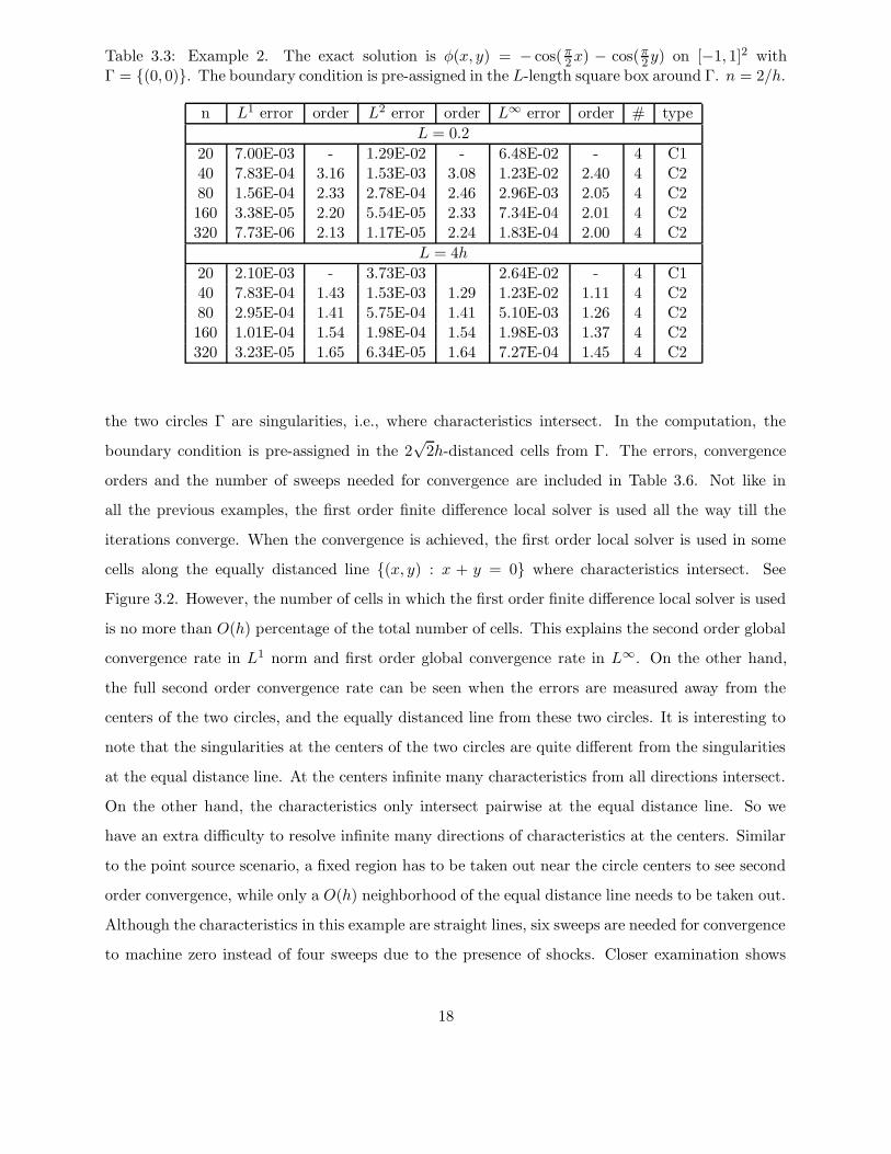
Table 3.3: Example 2. The exact solution is φ(x, y) = − cos( π2x) − cos(π

2 y) on [−1, 1]2 withΓ = (0, 0). The boundary condition is pre-assigned in the L-length square box around Γ. n = 2/h.


L = 0.2


L = 4h

20 2.10E-03 - 3.73E-03 2.64E-02 - 4 C140 7.83E-04 1.43 1.53E-03 1.29 1.23E-02 1.11 4 C280 2.95E-04 1.41 5.75E-04 1.41 5.10E-03 1.26 4 C2160 1.01E-04 1.54 1.98E-04 1.54 1.98E-03 1.37 4 C2320 3.23E-05 1.65 6.34E-05 1.64 7.27E-04 1.45 4 C2

the two circles Γ are singularities, i.e., where characteristics intersect. In the computation, the

boundary condition is pre-assigned in the 2√

2h-distanced cells from Γ. The errors, convergence

orders and the number of sweeps needed for convergence are included in Table 3.6. Not like in

all the previous examples, the first order finite difference local solver is used all the way till the

iterations converge. When the convergence is achieved, the first order local solver is used in some

cells along the equally distanced line (x, y) : x + y = 0 where characteristics intersect. See

Figure 3.2. However, the number of cells in which the first order finite difference local solver is used

is no more than O(h) percentage of the total number of cells. This explains the second order global

convergence rate in L1 norm and first order global convergence rate in L∞. On the other hand,

the full second order convergence rate can be seen when the errors are measured away from the

centers of the two circles, and the equally distanced line from these two circles. It is interesting to

note that the singularities at the centers of the two circles are quite different from the singularities

at the equal distance line. At the centers infinite many characteristics from all directions intersect.

On the other hand, the characteristics only intersect pairwise at the equal distance line. So we

have an extra difficulty to resolve infinite many directions of characteristics at the centers. Similar

to the point source scenario, a fixed region has to be taken out near the circle centers to see second

order convergence, while only a O(h) neighborhood of the equal distance line needs to be taken out.

Although the characteristics in this example are straight lines, six sweeps are needed for convergence

to machine zero instead of four sweeps due to the presence of shocks. Closer examination shows

18

Table 3.4: Example 2. Convergence of the gradient of φh to ∇φ. The exact solution is φ(x, y) =− cos(π

2x) − cos(π2 y) on [−1, 1]2 with Γ = (0, 0). The boundary condition is pre-assigned in the

L-length square box around Γ. n = 2/h.

n L1 error order L2 error order L∞ error order

L = 0.2

20 1.36E-01 - 1.47E-01 - 4.54E-01 -40 5.21E-02 1.38 5.42E-02 1.44 2.11E-01 1.1180 2.41E-02 1.11 2.40E-02 1.18 1.06E-01 0.99160 1.16E-02 1.05 1.12E-02 1.10 5.29E-02 1.00320 5.68E-03 1.03 5.38E-03 1.06 2.65E-02 1.00

L = 4h

20 1.02E-01 - 1.03E-01 3.36E-01 -40 5.21E-02 0.97 5.42E-02 0.92 2.11E-01 0.6780 2.59E-02 1.01 2.75E-02 0.98 1.27E-01 0.73160 1.27E-02 1.03 1.36E-02 1.02 7.41E-02 0.78320 6.19E-03 1.04 6.56E-03 1.05 4.24E-02 0.81

that by the end of the fourth sweep, the solution is settled everywhere except in a few cells near

the shock location. Such cells are among those which eventually involve the first order local solver

when the convergence is achieved, see Figure 3.2. Similar phenomenon occurs for the first order

monotone scheme although the accuracy has already been achieved after four iterations, i.e., the

modifications to balance information from different characteristics near shocks after four iterations

are really small compared to the approximation error of the discretization scheme. This is discussed

in [54].

Compared to the results in Table 3.7 using first order scheme [54], we see that the global L∞

error is comparable. This is due to the fact that the first order local solver is used in certain cells,

e.g., near the shocks. As shown by a constructed example in [54], at most first order accuracy can

be achieved in L∞ norm at the shock location. However, for the integral L1 or L2 norm we see

a higher order of convergence and much smaller error than the first order scheme even including

those singularities. This is due to the fact that the number of cells in which the first order local

solver is used is no more than O(h) percentage of the number of the total cells.

Example 5 (shape-from-shading): Ω = [−1, 1]2, Γ = ∂Ω. The solution of this example is the

shape function, which has the brightness I(x, y) = 1/√

1 + f(x, y)2 under vertical lighting. See [41]

for details. We consider the following two cases:

19

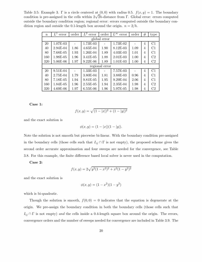
Table 3.5: Example 3. Γ is a circle centered at (0, 0) with radius 0.5. f(x, y) = 1. The boundarycondition is pre-assigned in the cells within 2

√2h-distance from Γ. Global error: errors computed

outside the boundary condition region; regional error: errors computed outside the boundary con-dition region and outside the 0.1-length box around the origin. n = 2/h.


global error


regional error


Case 1:

f(x, y) =√

(1 − |x|)2 + (1 − |y|)2

and the exact solution is

φ(x, y) = (1 − |x|)(1 − |y|).

Note the solution is not smooth but piecewise bi-linear. With the boundary condition pre-assigned

in the boundary cells (those cells such that Iij ∩ Γ is not empty), the proposed scheme gives the

second order accurate approximation and four sweeps are needed for the convergence, see Table

3.8. For this example, the finite difference based local solver is never used in the computation.

Case 2:

f(x, y) = 2√

y2(1 − x2)2 + x2(1 − y2)2

and the exact solution is

φ(x, y) = (1 − x2)(1 − y2)

which is bi-quadratic.

Though the solution is smooth, f(0, 0) = 0 indicates that the equation is degenerate at the

origin. We pre-assign the boundary condition in both the boundary cells (those cells such that

Iij ∩ Γ is not empty) and the cells inside a 0.4-length square box around the origin. The errors,

convergence orders and the number of sweeps needed for convergence are included in Table 3.9. The

20

−1 −0.8 −0.6 −0.4 −0.2 0 0.2 0.4 0.6 0.8 1−1

−0.8

−0.6

−0.4

−0.2

0

0.2

0.4

0.6

0.8

1

x

y

n=20

−1 −0.8 −0.6 −0.4 −0.2 0 0.2 0.4 0.6 0.8 1−1

−0.8

−0.6

−0.4

−0.2

0

0.2

0.4

0.6

0.8

1

x

y

n=40

−1 −0.8 −0.6 −0.4 −0.2 0 0.2 0.4 0.6 0.8 1−1

−0.8

−0.6

−0.4

−0.2

0

0.2

0.4

0.6

0.8

1

x

y

n=80

−1 −0.8 −0.6 −0.4 −0.2 0 0.2 0.4 0.6 0.8 1−1

−0.8

−0.6

−0.4

−0.2

0

0.2

0.4

0.6

0.8

1

x

y

n=160

Figure 3.2: Example 4. The location of those cells where the first order local solver is used by thetime the convergence is achieved.

results show that the method is second order accurate, and the convergence is achieved quickly. In

the computation, the finite difference type local solver is used before the convergence is achieved,

and it is never used afterward.

In Figure 3.3, we plot the numerical solutions φh on the 80× 80 mesh for both the smooth and

non-smooth examples.

Example 6 (shape-from-shading): Ω = [0, 1]2, Γ = ∂Ω ∪ ( 14 ,

14), (1

4 ,34), (3

4 ,14), (3

4 ,34 ), (1

2 ,12 ), and

f(x, y) = 2π

√

cos2(2πx) sin2(2πy) + sin2(2πx) cos2(2πy).

The solution for this problem is the shape function, which has the brightness I(x, y) = 1/√

1 + f(x, y)2

under vertical lighting. See [41] for details. On Γ, φ(x, y) = g(x, y) is given with the following two

choices:

Case 1:

g(x, y) =

0, (x, y) ∈ ∂Ω ∪ (1/2, 1/2)1, (x, y) ∈ (1/4, 1/4), (3/4, 3/4)

−1, (x, y) ∈ (1/4, 3/4), (3/4, 1/4)

21

Table 3.6: Example 4. Γ consists of two circles with centers (0.5, 0.5), (−0.5,−0.5) and the radiusRs = 0.3. f(x, y) = 1. The boundary condition is pre-assigned in the cells within 2

√2h-distance

from Γ. Global error: errors computed outside the boundary condition region; regional error:errors computed in the cells 2

√2h distance away from the equally distanced line from the circles,

0.1 distance away from the circle centers, and outside the boundary condition region. †= thepercentage of the cells in which the finite difference type local solver is used by the time theiterations converge. n = 2/h.

n L1 error order L2 error order L∞ error order # type †global error

20 2.75E-03 - 6.80E-03 - 7.20E-02 - 6 C3 1.000%40 6.59E-04 2.06 1.97E-03 1.79 3.66E-02 0.98 6 C3 1.250%80 1.63E-04 2.02 6.30E-04 1.64 1.84E-02 0.99 6 C3 0.438%160 4.08E-05 2.00 2.11E-04 1.58 9.25E-03 0.99 6 C3 0.250%320 1.03E-05 1.99 7.26E-05 1.54 4.63E-03 1.00 6 C3 0.137%

regional error

20 9.74E-04 - 1.14E-03 - 3.16E-03 - 6 C3 1.000%40 3.49E-04 1.48 4.74E-04 1.27 3.84E-03 - 6 C3 1.250%80 9.09E-05 1.94 1.24E-04 1.93 9.31E-04 2.04 6 C3 0.438%160 2.33E-05 1.96 3.23E-05 1.94 2.37E-04 1.97 6 C3 0.250%320 5.90E-06 1.98 8.29E-06 1.96 6.03E-05 1.97 6 C3 0.137%

The exact solution for this case is a smooth function:

φ(x, y) = sin(2πx) sin(2πy).

Case 2:

g(x, y) =

0, (x, y) ∈ ∂Ω1, (x, y) ∈ (1/4, 1/4), (1/4, 3/4), (3/4, 1/4), (3/4, 3/4)2, (x, y) ∈ (1/2, 1/2)

The exact solution for this case is

φ(x, y) =

1 + cos(2πx) cos(2πy), if |x+ y − 1| < 1/2, and |x− y| < 1/2| sin(2πx) sin(2πy)|, otherwise

which is non-smooth.

For these two cases, the boundary conditions are pre-assigned in the cells right next to the

domain boundary, and in the cells within a 0.1-length square box around each isolated point in Γ.

The results are reported in Table 3.10 and Table 3.11, and the numerical solutions on the 80 × 80

mesh are presented in Figure 3.4. For these examples, the first order finite difference local solver is

used all the way till the iterations converge. When the convergence is achieved, the number of cells

in which the first order finite difference local solver is still used is no more than O(h) percentage of

22

Table 3.7: Example 4. Γ consists of two circles with centers (0.5, 0.5), (−0.5,−0.5) and the radiusRs = 0.3. f(x, y) = 1. The boundary condition is pre-assigned in the cells within 2

√2h-distance

from Γ. The computation is by the first order Godunov finite difference fast sweeping method.n = 2/h.



Table 3.8: Example 5. Shape-from-shading, the non-smooth example. The boundary condition ispre-assigned in the boundary cells. n = 2/h.



the number of the total cells. This means, asymptotically, the local solver is second order accurate,

and this explains the second order convergence rates in L1 norm in Table 3.10 and Table 3.11. On

the other hand, the existence of a O(h)-size region in which the first order finite difference based

local solver is used explains the lower-than-second-order convergence rates in L2 and L∞ norms.

In both examples, the number of sweeps needed for the convergence is fairly small.

Similar to what we have seen in Example 4, although the first order local solver is used in certain

cells when the convergence is achieved, our essentially second order accurate algorithm produces

more accurate approximations than the first order Godunov finite difference fast sweeping method

[54], see Table 3.12.

Example 7: Finally in this section, we want to use one example to show that it is necessary to

check the signs of unewij and vnew

ij in the local solver in Section 2.1 and Section 2.2 in order to decide

which solution candidate should be accepted on Iij .

We consider the example with the exact solution φ(x, y) = sin( π2x) on Ω = [0, 1]2, Γ =

(x, y) | x = 0. The results computed with and without checking the sign of unewij and vnew

ij

23

−1

−0.5

0

0.5

1

−1

−0.5

0

0.5

10

0.2

0.4

0.6

0.8

1

xy

φ h

−1

−0.5

0

0.5

1

−1

−0.5

0

0.5

10

0.2

0.4

0.6

0.8

1

xy

φ h

Figure 3.3: Example 5. φh in Shape-from-shading. The left one is for case 1, the non-smoothexample and the right one is for case 2, the smooth example. n = 2/h = 80.

Table 3.9: Example 5. Shape-from-shading, the smooth example. The boundary condition is pre-assigned in both the boundary cells and the cells in the 0.4-length square box in the center of thedomain. n = 2/h.



are included in Figure 3.5 and Figure 3.6. One can see that without checking the sign of the deriva-

tive of φh (using either the hybrid local solver, or the pure DG local solver), the wrong candidate

will be picked up. The plots for 1D cut of the φij and uij/h with fixed y in Figure 3.6 show what

actually happens.

4 Concluding Remarks

We have developed a fast sweeping method based on a discontinuous Galerkin (DG) local solver for

computing viscosity solutions of a class of static Hamilton-Jacobi equations, namely the Eikonal

equations on rectangular grids. The compactness of the local DG solver matches well with the fast

sweeping strategy, a Gauss-Seidel type of iterated method, to provide both accuracy and efficiency,

which is demonstrated by extensive numerical tests. Extension to higher dimensions, higher order

DG solvers, and non-uniform/triangular meshes will be studied in the future. In three dimensional

case, the local solver is still very simple. We believe the advantage over first order scheme will be

24

Table 3.10: Example 6. Shape-from-shading, the smooth example. The boundary condition is pre-assigned in the cells right next to the domain boundary and in the 0.1-length square box aroundthe isolated points in Γ. †= the percentage of the cells in which the finite difference type localsolver is used by the time the iterations converge. n = 1/h.

n L1 error order L2 error order L∞ error order # type †20 1.08E-02 - 1.84E-02 - 1.20E-01 - 8 C3 3.000%40 1.91E-03 2.50 4.30E-03 2.10 5.38E-02 1.15 7 C3 1.750%80 4.47E-04 2.09 1.34E-03 1.68 2.67E-02 1.01 12 C3 1.250%160 1.09E-04 2.04 4.51E-04 1.57 1.32E-02 1.01 15 C3 0.547%320 2.71E-05 2.01 1.54E-04 1.55 6.60E-03 1.00 16 C3 0.270%

Table 3.11: Example 6. Shape-from-shading, the non-smooth example. The boundary conditionis pre-assigned in the cells right next to the domain boundary and in the 0.1-length square boxaround the isolated points in Γ. †= the percentage of the cells in which the finite difference typelocal solver is used by the time the iterations converge. n = 1/h.

n L1 error order L2 error order L∞ error order # type †20 9.40E-03 - 1.16E-02 - 4.94E-02 - 7 C3 2.000%40 2.70E-03 1.80 4.60E-03 1.33 5.13E-02 - 11 C3 2.000%80 6.83E-04 1.99 1.16E-03 1.99 1.41E-02 1.87 11 C3 0.188%160 1.87E-04 1.87 4.23E-04 1.46 4.67E-03 1.59 15 C3 0.094%320 5.19E-05 1.85 1.48E-04 1.51 2.07E-03 1.17 15 C3 0.039%

more significant in higher dimensions. In order to develop the higher order DG based fast sweeping

methods, one would need to first overcome the use of the first order solver in the DG local solver.

The success of the fast sweeping method on triangular meshes in [38] may assist us to design the

DG based fast sweeping methods for more general meshes.

References

[1] R. Abgrall, Numerical discretization of the first-order Hamilton-Jacobi equation on triangular

meshes, Communications on Pure and Applied Mathematics, 49 (1996), 1339–1373.

[2] D.N. Arnold, F. Brezzi, B. Cockburn, and L.D. Marini, Unified analysis of discontinuous

Galerkin methods for elliptic problems, SIAM Journal on Numerical Analysis, 39 (2001/02),

1749–1779.

[3] S. Augoula and R. Abgrall, High order numerical discretization for Hamilton-Jacobi equations

on triangular meshes, Journal of Scientific Computing, 15 (2000), 197–229.

25

Table 3.12: Example 6. Shape-from-shading, both smooth and non-smooth examples. The bound-ary condition is pre-assigned in the cells right next to the domain boundary and in the 0.1-lengthsquare box around the isolated points in Γ. The computation is by the first order Godunov finitedifference fast sweeping method. n = 1/h.


smooth example


non-smooth example


[4] T. Barth and J. Sethian, Numerical schemes for the Hamilton-Jacobi and level set equations

on triangulated domains, Journal of Computational Physics, 145 (1998), 1–40.

[5] M. Boue and P. Dupuis, Markov chain approximations for deterministic control problems with

affine dynamics and quadratic cost in the control, SIAM Journal on Numerical Analysis, 36

(1999), 667–695.

[6] S. Bryson and D. Levy, High-order central WENO schemes for multidimensional Hamilton-

Jacobi equations, SIAM Journal on Numerical Analysis, 41 (2003), 1339–1369.

[7] T. Cecil, J. Qian and S. Osher, Numerical methods for high dimensional Hamilton-Jacobi

equations using radial basis functions, Journal of Computational Physics, 196 (2004), 327–347.

[8] L.-T. Cheng and Y.-H. Tsai, Redistancing by flow of time dependent Eikonal equation, UCLA

CAM Report 07-16.

[9] Y. Cheng and C.-W. Shu, A discontinuous Galerkin finite element method for directly solving

the Hamilton-Jacobi equations. Journal of Computational Physics, 223 (2007), 398–415.

[10] B. Cockburn, S. Hou and C.-W. Shu, The Runge-Kutta local projection discontinuous Galerkin

finite element method for conservation laws IV: the multidimensional case, Mathematics of

Computation, 54 (1990), 545–581.

26

00.2

0.40.6

0.81

0

0.2

0.4

0.6

0.8

1−1

−0.5

0

0.5

1

xy

φ h

00.2

0.40.6

0.81

0

0.2

0.4

0.6

0.8

10

0.5

1

1.5

2

xy

φ h

Figure 3.4: Example 6. φh in Shape-from-shading. The left one is for the smooth solution and theright one is for the non-smooth one. n = 1/h = 80.

[11] B. Cockburn, S.-Y. Lin and C.-W. Shu, TVB Runge-Kutta local projection discontinuous

Galerkin finite element method for conservation laws III: one dimensional systems, Journal

of Computational Physics, 84 (1989), 90–113.

[12] B. Cockburn and C.-W. Shu, TVB Runge-Kutta local projection discontinuous Galerkin finite

element method for conservation laws II: general framework, Mathematics of Computation, 52

(1989), 411–435.

[13] B. Cockburn and C.-W. Shu, The Runge-Kutta discontinuous Galerkin method for conservation

laws V: multidimensional systems, Journal of Computational Physics, 141 (1998), 199–224.

[14] B. Cockburn and C.-W. Shu, The local discontinuous Galerkin method for time-dependent

convection-diffusion systems, SIAM Journal on Numerical Analysis, 35 (1998), 2440–2463.

[15] B. Cockburn and C.-W. Shu, Runge-Kutta discontinuous Galerkin methods for convection-

dominated problems, Journal of Scientific Computing, 16 (2001), 173–261.

[16] M.G. Crandall and P.L. Lions, Viscosity solutions of Hamilton-Jacobi equations, Transactions

of American Mathematical Society, 277 (1983), 1–42.

[17] J. Dellinger and W.W. Symes, Anisotropic finite-difference traveltimes using a Hamilton-Jacobi

solver, 67th Ann. Internat. Mtg., Soc. Expl. Geophys., Expanded Abstracts, 1997, 1786–1789.

[18] E. W. Dijkstra, A note on two problems in connection with graphs, Numerische Mathematik,

1 (1959), 269–271.

27

[19] M. Falcone and R. Ferretti, Discrete time high-order schemes for viscosity solutions of

Hamilton-Jacobi-Bellman equations, Numerische Mathematik, 67 (1994), 315–344.

[20] M. Falcone and R. Ferretti, Semi-Lagrangian schemes for Hamilton-Jacobi equations, discrete

representation formulae and Godunov methods, Journal of Computational Physics, 175 (2002),

559–575.

[21] S. Gray and W. May, Kirchhoff migration using Eikonal equation travel-times, Geophysics, 59

(1994), 810–817.

[22] J. Helmsen, E. Puckett, P. Colella and M. Dorr, Two new methods for simulating photolithog-

raphy development in 3D, Proceedings SPIE 2726 (1996), 253–261.

[23] C. Hu, O. Lepsky and C.-W. Shu, The effect of the least square procedure for discontinuous

Galerkin methods for Hamilton-Jacobi equations. Discontinuous Galerkin methods (Newport,

RI, 1999), Lecture Notes in Computational Science and Engineering, Springer, Berlin, 2000.

343–348.

[24] C. Hu and C.-W. Shu, A discontinuous Galerkin finite element method for Hamilton-Jacobi

equations, SIAM Journal on Scientific Computing, 20 (1999), 666–690.

[25] G.-S. Jiang and D. Peng, Weighted ENO schemes for Hamilton-Jacobi equations, SIAM Journal

on Scientific Computing, 21 (2000), 2126–2143.

[26] S. Jin and Z. Xin, Numerical passage from systems of conservation laws to Hamilton-Jacobi

equations and relaxation schemes, SIAM Journal on Numerical Analysis, 35 (1998), 2385–2404.

[27] C.Y. Kao, S. Osher and J. Qian, Lax-Friedrichs sweeping schemes for static Hamilton-Jacobi

equations, Journal of Computational Physics, 196 (2004), 367–391.

[28] C.Y. Kao, S. Osher and Y.H. Tsai, Fast sweeping method for static Hamilton-Jacobi equations,

SIAM Journal on Numerical Analysis, 42 (2005), 2612–2632.

[29] S. Kim and R. Cook, 3D traveltime computation using second-order ENO scheme, Geophysics,

64 (1999), 1867–1876.

[30] F. Li and C.-W. Shu, Reinterpretation and simplified implementation of a discontinuous

Galerkin method for Hamilton-Jacobi equations, Applied Mathematics Letters, 18 (2005),

1204–1209.

28

[31] C.-T. Lin and E. Tadmor, High-resolution non-oscillatory central schemes for approximate

Hamilton-Jacobi equations, SIAM Journal on Scientific Computing, 21 (2000), 2163–2186.

[32] S. Osher, A level set formulation for the solution of the Dirichlet problem for Hamilton-Jacobi

equations, SIAM Journal on Mathematical Analysis, 24 (1993), 1145–1152.

[33] S. Osher and J. Sethian, Fronts propagating with curvature dependent speed: algorithms based

on Hamilton-Jacobi formulations, Journal of Computational Physics, 79 (1988), 12–49.

[34] S. Osher and C.-W. Shu, High-order essentially nonoscillatory schemes for Hamilton-Jacobi

equations, SIAM Journal on Numerical Analysis, 28 (1991), 907–922.

[35] D. Peng, S. Osher, B. Merriman, H.-K. Zhao and M. Rang, A PDE-based fast local level set

method, Journal of Computational Physics, 155 (1999), 410–438.

[36] J. Qian and W.W. Symes, Paraxial Eikonal solvers for anisotropic quasi-P travel times, Journal

of Computational Physics, 174 (2001), 256–278.

[37] J. Qian and W.W. Symes, Finite-difference quasi-P traveltimes for anisotropic media, Geo-

physics, 67 (2002), 147–155.

[38] J. Qian, Y.-T. Zhang and H.-K. Zhao, Fast sweeping methods for Eikonal equations on trian-

gular meshes, SIAM Journal on Numerical Analysis, 45 (2007), 83–107.

[39] J. Qian, Y.-T. Zhang and H.-K. Zhao, A fast sweeping method for static convex Hamilton-

Jacobi equations, Journal of Scientific Computing, 31 (2007), 237–271.

[40] C. Rasch and T. Satzger, Remarks on the O(N) implementation of the fast marching method,

submitted.

[41] E. Rouy and A. Tourin, A viscosity solutions approach to shape-from-shading, SIAM Journal

on Numerical Analysis, 29 (1992), 867–884.

[42] W.H. Reed and T.R. Hill, Triangular mesh method for the neutron transport equation, Tech-

nical report LA-UR-73-479, Los Alamos Scientific Laboratory, Los Alamos, NM, 1973.

[43] J.A. Sethian, A fast marching level set method for monotonically advancing fronts, Proceedings

of the National Academy of Sciences of the United States of America, 93 (1996), 1591–1595.

29

[44] J.A. Sethian and A. Vladimirsky, Ordered upwind methods for static Hamilton-Jacobi equa-

tions, Proceedings of the National Academy of Sciences of the United States of America, 98

(2001), 11069–11074.

[45] J.A. Sethian and A. Vladimirsky, Ordered upwind methods for static Hamilton-Jacobi equa-

tions: theory and algorithms, SIAM Journal on Numerical Analysis, 41 (2003), 325–363.

[46] C.-W. Shu, High order numerical methods for time dependent Hamilton-Jacobi equations, IMS

Lecture Notes Series, Vol 11: Mathematics and Computation in Imaging Science and Infor-

mation Processing, World Scientific Publishing, Singapore, 2007, 47–91.

[47] Y.-H. R. Tsai, L.-T. Cheng, S. Osher and H.-K. Zhao, Fast sweeping algorithms for a class of

Hamilton-Jacobi equations, SIAM Journal on Numerical Analysis, 41 (2003), 673–694.

[48] J.N. Tsitsiklis, Efficient algorithms for globally optimal trajectories, IEEE Transactions on

Automatic Control, 40 (1995), 1528–1538.

[49] J. Yan and C.-W. Shu, A local discontinuous Galerkin method for KdV type equations, SIAM

Journal on Numerical Analysis, 40 (2002), 769–791.

[50] L. Yatziv, A. Bartesaghi and G. Sapiro, O(N) implementation of the fast marching algorithm,

Journal of Computational Physics, 212 (2006), 393–399.

[51] Y.-T. Zhang and C.-W. Shu, High order WENO schemes for Hamilton-Jacobi equations on

triangular meshes, SIAM Journal on Scientific Computing, 24 (2003), 1005–1030.

[52] Y.-T. Zhang, H.-K. Zhao and S. Chen, Fixed-point iterative sweeping methods for static

Hamilton-Jacobi equations, Methods and Applications of Analysis, 13 (2006), 299–320.

[53] Y.-T. Zhang, H.-K. Zhao and J. Qian, High order fast sweeping methods for static Hamilton-

Jacobi equations, Journal of Scientific Computing, 29 (2006), 25–56.

[54] H.-K. Zhao, A fast sweeping method for Eikonal equations. Mathematics of Computation, 74

(2005), 603–627.

[55] H. Zhao, S. Osher, B. Merriman and M. Kang, Implicit and non-parametric shape reconstruc-

tion from unorganized points using variational level set method, Computer Vision and Image

Understanding, 80 (2000), 295–319.

30

00.2

0.40.6

0.81

0

0.2

0.4

0.6

0.8

10

0.2

0.4

0.6

0.8

1

xy

φ h

00.2

0.40.6

0.81

0

0.2

0.4

0.6

0.8

10

0.5

1

1.5

2

xy

φ hx

00.2

0.40.6

0.81

0

0.2

0.4

0.6

0.8

10

0.2

0.4

0.6

0.8

1

xy

φ h

00.2

0.40.6

0.81

0

0.2

0.4

0.6

0.8

1−2

−1.5

−1

−0.5

0

0.5

1

1.5

2

xy

φ hx

00.2

0.40.6

0.81

0

0.2

0.4

0.6

0.8

10

0.2

0.4

0.6

0.8

1

xy

φ h

00.2

0.40.6

0.81

0

0.2

0.4

0.6

0.8

1−2

−1.5

−1

−0.5

0

0.5

1

1.5

2

xy

φ hx

Figure 3.5: Justification for the necessity of checking the signs of unewij and vnew

ij in the local solverin Section 2.1 and 2.2. The exact solution is φ(x, y) = sin( π

2x). φh is computed when the signs ofuij and vij are checked (top), when the signs are not checked (middle), and when the signs are notchecked and the pure DG local solver is used (bottom). Left: φij ; Right: uij/h. n = 1/h = 40.

31

0 0.1 0.2 0.3 0.4 0.5 0.6 0.7 0.8 0.9 10

0.1

0.2

0.3

0.4

0.5

0.6

0.7

0.8

0.9

1

x

φ h

with, hybrid

without

without, hybrid

0 0.1 0.2 0.3 0.4 0.5 0.6 0.7 0.8 0.9 1−2

−1.5

−1

−0.5

0

0.5

1

1.5

2

x

φ hx

with, hybrid

without

without, hybrid

Figure 3.6: Justification for the necessity of checking the signs of unewij and vnew

ij in the local solver

in Section 2.1 and 2.2. The exact solution is φ(x, y) = sin( π2x). The 1D cut of φij (left) and uij/h

(right). φh is computed when the signs of uij and vij are checked (with, hybrid), when the signs arenot checked (without, hybrid), and when the signs are not checked and the pure DG local solver isused (without). n = 1/h = 40.

32

a second order discontinuous galerkin fast sweeping method...

Documents