A S D F : Automated, Online Fingerpointingfor Hadoop1

Keith Bare, Michael P. Kasick, Soila Kavulya, Eugene Marinelli,Xinghao Pan, Jiaqi Tan,

Rajeev Gandhi, Priya Narasimhan

CMU-PDL-08-104

May 2008

Parallel Data LaboratoryCarnegie Mellon UniversityPittsburgh, PA 15213-3890

Abstract

Localizing performance problems (or fingerpointing) is essential for distributed systems such as Hadoop that support long-running,parallelized, data-intensive computations over a large cluster of nodes. Manual fingerpointing does not scale in such environmentsbecause of the number of nodes and the number of performance metrics to be analyzed on each node. ASDF is an automated, onlinefingerpointing framework that transparently extracts and parses different time-varying data sources (e.g., sysstat, Hadoop logs)on each node, and implements multiple techniques (e.g., log analysis, correlation, clustering) to analyze these data sources jointlyor in isolation. We demonstrate ASDF’s online fingerpointing for documented performance problems in Hadoop, under differentworkloads; our results indicate that ASDF incurs an average monitoring overhead of 0.38% of CPU time, and exhibits averageonline fingerpointing latencies of less than 1 minute with false-positive rates of less than 1%.

1ASDF stands for Automated System for Diagnosing FailuresAcknowledgements: The authors would like to acknowledge Julio Lopez for discussions on Hadoop, Kathleen Carley for her insights on

visualization, and Christos Faloutsos for discussions on data mining. This material is based on research sponsored in part by the National ScienceFoundation, via CAREER grant CCR-0238381 and grant CNS-0326453.

Keywords: problem diagnosis, hadoop

1 Introduction

Distributed systems are typically composed of communicating components that are spatially distributedacross nodes in the system. Performance problems in such systems can be hard to diagnose and to local-ize to a specific node or a set of nodes. There are many challenges in problem localization (i.e., tracingthe problem back to the original culprit node or nodes) and root-cause analysis (i.e., tracing the problemfurther to the underlying code-level fault or bug, e.g., memory leak, deadlock). First, performance prob-lems can originate at one node in the system and then start to manifest at other nodes as well, due to theinherent communication across components–this can make it hard to discover the original culprit node.Second, performance problems can change in their manifestation over time–what originally manifests as amemory-exhaustion problem can ultimately escalate to resemble a node crash, making it hard to discoverthe underlying root-cause of the problem. Obviously, the larger the system and the more complex anddistributed the interactions, the more difficult it is to diagnose the origin and root-cause of a problem.

Problem-diagnosis techniques tend to gather data about the system and/or the application to develop apriori templates of normal, problem-free system behavior; the techniques then detect performance problemsby looking for anomalies in runtime data, as compared to the templates. Typically, these analysis techniquesfor anomaly detection and diagnosis are run offline and post-process the data gathered from the system. Thedata used to develop the models and to perform the diagnosis can be collected in different ways.

A white-box diagnostic approach extracts application-level data directly and requires instrumentingthe application and possibly understanding the application’s internal structure or semantics. A black-boxdiagnostic approach aims to infer application behavior by extracting data transparently from the operatingsystem or network without needing to instrument the application or to understand its internal structure orsemantics. Obviously, it might not be scalable (in effort, time and cost) or even possible to employ a white-box approach in production environments that contain many third-party services, applications and users. Ablack-box approach also has its drawbacks–while such an approach can infer application behavior to someextent, it might not always be able to pinpoint the root cause of a performance problem. Typically, a black-box approach is more effective at problem localization, while a white-box strategy can be implemented toextract more information to ascertain the underlying root cause of a problem.

There are two distinct problems that we pursued. First, we sought to address support for problemlocalization (what we call fingerpointing) online, in an automated manner, even as the system under diag-nosis is running. Second, we sought to address the problem of automated fingerpointing for Hadoop [9],an open-source implementation of the MapReduce programming paradigm [6] that supports long-running,parallelized, data-intensive computations over a large cluster of nodes.

This paper describes ASDF, a flexible, online framework for fingerpointing that addresses the two prob-lems outlined above. ASDF has API support to plug in different time-varying data sources, and to plug invarious analysis modules to process this data. Both the data-collection and the data-analyses can proceedconcurrently, while the system under diagnosis is executing. The data sources can be gathered in either ablack-box or white-box manner, and can be diverse, coming from application logs, system-call traces, sys-tem logs, performance counters, etc. The analysis modules can be equally diverse, involving time-seriesanalysis, machine learning, etc.

We demonstrate how ASDF automatically fingerpoints some of the performance problems in Hadoopthat are documented in Apache’s JIRA issue tracker [8]. Manual fingerpointing does not scale in Hadoopenvironments because of the number of nodes and the number of performance metrics to be analyzed on eachnode. Our current implementation of ASDF for Hadoop automatically extracts time-varying black-box datasources (sysstat: sadc and pidstat) and specific white-box data sources (Hadoop logs) on every node in aHadoop cluster. ASDF then feeds these data sources into different analysis modules (that respectively performclustering, peer-comparison or Hadoop-log analysis), to identify the culprit node(s), in real time. A uniqueaspect of our Hadoop-centric fingerpointing is our ability to infer Hadoop states (as we chose to define them)

1

by parsing the logs that are natively auto-generated by Hadoop. We then leverage the information about thestates and the time-varying state-transition sequence to localize performance problems.

There is considerable related work in the area of both instrumentation/monitoring as well as in problem-diagnosis techniques, as described in Section 6. To the best of our knowledge, ASDF is the first automated,online problem-localization framework that is designed to be flexible in its architecture by supporting theplugging-in of data sources and analysis techniques. As far as we know, ASDF is also the first to demon-strate the online diagnosis of problems in Hadoop, without requiring modifications to Hadoop or to anyapplications that Hadoop supports. Specifically, for Hadoop, ASDF addresses the operational challengesof performing the analysis online, while dealing with multiple data-sources (black-box and white-box) ofvarying rates.

2 Problem Statement

The aim of ASDF is to assist system administrators in identifying the culprit node(s) when the system experi-ences a performance problem. The research questions center around whether ASDF can localize performanceproblems quickly, accurately and non-invasively. In addition, performing online fingerpointing in the con-text of Hadoop presents its own unique challenges. While we choose to demonstrate ASDF’s capabilitiesfor Hadoop in this paper, we emphasize that (with the appropriate combination of data sources and analysismodules) ASDF is generally applicable to problem localization in any distributed system.

2.1 Goals

We impose the following requirements for ASDF to meet its stated objectives.

Runtime data collection. ASDF should allow system administrators to leverage any available data source(black-box or white-box) in the system. No restrictions should be placed on the rate at which data can becollected from a specific data-source.

Runtime data analysis. ASDF should allow system administrators to leverage custom or off-the-shelf anal-ysis techniques. The data-analysis techniques should process the incoming, real-time data to determinewhether the system is experiencing a performance problem, and if so, to produce a list of possible culpritnode(s). No restrictions should be placed on the type of analysis technique that can be plugged in.

Performance. ASDF should produce low false-positive rates, in the face of a variety of workloads for thesystem under diagnosis, and more importantly, even in the face of workload changes at runtime1. The ASDFframework’s data-collection should impose minimal runtime overheads on the system under diagnosis. Inaddition, ASDF’s data-analysis should result in low fingerpointing latencies (where we define fingerpointinglatency as a measure of how quickly the framework identifies the culprit node(s) at runtime, once the problemis present in the system).

We impose the additional requirements below to make ASDF more practical to use and deploy.

Flexibility. ASDF should have the flexibility to attach or detach any data source (white-box or black-box) thatis available in the system, and similarly, the flexibility to incorporate any off-the-shelf or custom analysismodule.

Operation in production environments. ASDF should run transparently to, and not require any modifica-

1The issue of false positives due to workload changes arises because workload changes can often be mistaken for anomalousbehavior, if the system’s behavior is characterized in terms of performance data such as CPU usage, network traffic, response times,etc. Without additional semantic information about the application’s actual execution or behavior, it can be difficult for a black-boxapproach, or even a white-box one, to distinguish legitimate workload changes from anomalous behavior.

2

Data-collection modules

Analysis modules

Administrator

fpt-core

Configurationfile

Figure 1: Logical architecture of ASDF.

tions of, both the hosted applications and any middleware that they might use. ASDF should be deployablein production environments, where administrators might not have the luxury of instrumenting applicationsbut could instead leverage other (black-box) data. In cases where applications are already instrumented toproduce logs of white-box data (as in Hadoop’s case) even in production environments, ASDF should exploitsuch data sources.

Offline and online analyses. While our primary goal is to support online automated fingerpointing, ASDFshould support offline analyses (for those users wishing to post-process the gathered data), effectively turn-ing itself into a data-collection and data-logging engine in this scenario.

2.2 Non-Goals

It is important to delineate the research results in this paper from possible extensions of this work. In itscurrent incarnation, ASDF is intentionally not focused on:

• Root-cause analysis: ASDF currently aims for (coarse-grained) problem localization by identifyingthe culprit node(s). Clearly, this differs from (fine-grained) root-cause analysis, which would aim toidentify the underlying fault or bug, possibly even down to the offending line of code.

• Performance tuning: ASDF does not currently attempt to develop performance models of the systemunder diagnosis, although ASDF does collect the data that could enable this capability.

3 Approach & Implementation

The central idea behind the ASDF framework is the ability to incorporate any number of different data sourcesin a distributed system and the ability to use any number of analysis techniques to process these data sources.We encapsulate distinct data sources and analysis techniques into modules. Modules can have both inputsand outputs. Most data-collection modules will tend to have only outputs, and no inputs because theycollect/sample data and supply it to other modules. On the other hand, analysis modules are likely to haveboth inputs (the data they are to analyze) and outputs (the fingerpointing outcome).

As an example on the data-collection side, ASDF currently supports a sadc module to collect datathrough the sysstatpackage, which contains various utilities to monitor system performance and usage

3

activity. There can be multiple module instances to handle multiple data sources of the same type. On theanalysis side, an example of a currently implemented module is mavgvec, which computes arithmetic meanand variance of a vector input over a sliding window of samples from multiple given input data streams.

3.1 Architecture

The key ASDF component, called the fpt-core (the “fingerpointing core”), serves as a multiplexer andprovides a plug-in API for which modules can be easily developed and integrated into the system. fpt-coreuses a directed acyclic graph (DAG) to model the flow of data between modules. Figure 1 shows the high-level logical architecture with ASDF’s different architectural elements–the fpt-core, its configuration fileand its attached data-collection and analysis modules. fpt-core incorporates a scheduler that dispatchesevents to the various modules that are attached to it.

Effectively, a specific configuration of the fpt-core (as defined in its configuration file) representsa specific way of wiring the data-collection modules to the analysis modules to produce a specific onlinefingerpointing tool. This is advantageous relative to a monolithic data-collection and analysis frameworkbecause fpt-core can be easily reconfigured to serve different purposes, e.g., to target the online diagnosisof a specific set of problems, to incorporate a new set of data sources, to leverage a new analysis technique,or to serve purely as a data-collection framework for post-processing of the data.

As described below, ASDF already incorporates a number of data-collection and analysis modules thatwe have implemented for reuse in other applications and systems. We believe that some of these modules(e.g., the sadc module) will be useful in many systems. It is possible for an ASDF user to leverage or extendthese existing modules to create a version of ASDF to suit his/her system under diagnosis. In addition, ASDF’sflexibility allows users to develop, and plug in, custom data-collection or analysis modules, to generate acompletely new online fingerpointing tool. For instance, an ASDF user can reconfigure the fpt-core and itsmodules to produce different instantiations of ASDF, e.g., a black-box version, a white-box version, or evena hybrid version that leverages both black- and white-box data for fingerpointing.

Because ASDF is intended to be deployed to diagnose problems in distributed systems, ASDF needsa way to extract data remotely from the data-collection modules on the nodes in the system and then toroute that data to the analysis modules. In the current incarnation of ASDF, we simplify this by running thefpt-core and the analysis modules on a single dedicated machine (called the ASDF control-node), and weperform the remote data collection using ONC RPC with protocol stubs generated by rpcgen [17]. For eachdata-collection module, abc, there exists a corresponding abc_rpcd counterpart that runs on the remotenode to gather the data that forms that module’s output.

3.2 Plug-in API for Implementing Modules

The fpt-core’s plug-in API was designed to be simple, yet generic. The API is used to create a module,which, when instantiated, will become a vertex in the DAG mentioned above. All types of modules–data-collection or analysis–use the same plug-in API, simplifying the implementation of the fpt-core.

A module’s init() function is called once each time that an instance of the module is created. Thisis where a module can perform any necessary per-instance initialization. Typical actions performed in amodule’s init() function include:

• Allocating module-specific instance data

• Reading configuration values from the section for the module instance

• Verifying that the number and type of input connections are appropriate

• Creating output connections for the module instance

4

• Setting origin information for the output connections

• Adding hooks that allow for the fpt-core’s scheduling of that module instance’s execution

• Performing any other module-specific initialization that is necessary.

A module’s run() function is called when the fpt-core’s scheduler determines that a module instanceshould run. One of the arguments to this function describes the reason why the module instance was run.If a module instance has inputs, it should read any data available on the inputs, and perform any necessaryprocessing. If a module instance has outputs, it should perform any necessary processing, and then writedata to the outputs.

3.3 Implementation of fpt-core

An ASDF user, typically a system administrator, would specify instances of modules in the fpt-core’sconfiguration file, along with module-specific configuration parameters (e.g., sampling interval for the datasource, threshold value for an analysis module’s anomaly-detection algorithm) along with a list of datainputs for each module. The fpt-core then uses the information in this configuration file to construct aDAG, with module instances as the graph’s vertices, and the graph’s edges represent the data flow from amodule’s outputs to another module’s inputs. Effectively, the DAG captures the “wiring diagram” betweenthe modules of the fpt-core at runtime.

The fpt-core’s runtime consists of two main phases, initialization and execution. As mentionedabove, the fpt-core’s inialization phase is responsible for parsing the fpt-core’s configuration file andconstructing the DAG of module instances. The DAG construction is perhaps the most critical aspect of theASDF online fingerpointing framework since it captures how data sources are routed to analysis techniquesat runtime.

1. In the first step of the DAG construction, fpt-core assigns a vertex in the DAG to each moduleinstance represented in the fpt-core’s configuration file.

2. Next, fpt-core annotates each module instance with its number of unsatisfied inputs. Those moduleswith fully satisfied inputs (i.e., output-only modules that specify no inputs) are added to a module-initialization queue.

3. For each module instance on the module-initialization queue, a new thread is spawned and the mod-ule’s init() function is called. The init() function verifies the module’s inputs, the modules’s config-uration parameters, and specifies its outputs. A module’s outputs, which are dynamically created atinitialization time, are then used to satisfy other module instances’ inputs. Whenever a new outputcauses all of the inputs of some other module instance to be satisfied, that module instance is placedon the queue.

4. The previous step is repeated until all of the modules’ inputs are satisfied, all of the threads are created,and all of the module instances are initalized. This should result in a successfully constructed DAG.If this (desirable) outcome is not achieved, then, it is likely that the fpt-core’s configuration wasincorrectly specified or that the right data-collection or analysis modules were not available. If thisoccurs, the fpt-core (and consequently, the ASDF) terminates.

Once the DAG is successfully constructed, the fpt-core enters its execution phase where it frequentlycalls each of the module instances’ run() function.

As part of the initialization process, module instances may request to be scheduled perodically, in whichcase their run() functions are called by the fpt-core’s scheduler at a fixed frequency. This allows the class

5

[ibuffer]

id = buf1

input[input] =

onenn0.output0

size = 10

[ibuffer]

id = buf2

input[input] =

onenn0.output0

size = 10

[ibuffer]

id = buf3

input[input] =

onenn0.output0

size = 10

[analysis_bb]

id = analysis

threshold = 5

window = 15

slide = 5

input[l0] = @buf0

input[l1] = @buf1

input[l2] = @buf2

input[l3] = @buf3

input[l4] = @buf4

[print]

id = BlackBoxAlarm

input[a] = @anal

Figure 2: A snippet from the fpt-core configuration file that we used for Hadoop, along with the corre-sponding DAG.

of data-collection modules (that typically have no specified inputs) to perodically poll external data sourcesand import their data values into the fpt-core.

For module instances with specified inputs (such as data-analysis modules), fpt-core automaticallyexecutes their run() functions each time that a configurable number of their inputs are updated with new datavalues. This enables data-analysis modules to perform any analysis immediately when the necessary data isavailable.

3.4 Configuring the fpt-core

Configuration files for the fpt-core have two purposes: they define the DAG that is used to perform prob-lem diagnosis and they specify any parameters processing modules may use. The format is straightforward.

A module is instantiated by specifying its name in square brackets. Following the name, parametervalues are assigned. The resulting module instance’s id can be specified with an assignment of the form “id= instance-id”. To build the graph, all of a module instance’s inputs must be specified as paremeters. Thisis done with assignments of the form “input[inputname] = instance-id.outputname” or “input[inputname] =@instance-id”. The former connects a single output, while the latter connects all outputs of the specifiedmodule instance. All other assignments are provided to the module instance for its own interpretation. Asnippet from the fpt-core configuration file that we used in our experiments with Hadoop, along with thecorresponding fpt-core DAG, are displayed in Figure 2.

3.5 Data-Collection Modules

Given the plug-in API described in Section 3.2, ASDF can support the inclusion of multiple data sources.Currently, ASDF supports the following data-collection modules: sadc and hadoop_log. We describe thesadc module below and the hadoop_log module in Section 4.4 (in order to explain its operation in thecontext of Hadoop).

The sadc Module. The sysstat package [20] comprises utilities (one of which is sadc) to monitor systemperformance and usage activity. System-wide metrics, such as CPU usage, context-switch rate, paging ac-

6

tivity, I/O activity, file usage, network activity (for specific protocols), memory usage, etc., are traditionallylogged in the /proc pseudo-filesystem and collected by /proc-parsing tools such as sadc and pidstat fromthe sysstat package. ASDF uses a modified version of the sysstat code in the form of a library, libsadc,which is capable of collecting system-wide and per-process statistics in the form of C data structures.

The ASDF sadc data-collection module exposes these /proc black-box metrics as fpt-core outputsand makes them available to the fpt-core’s analysis modules. We use Open Network Computing RemoteProcedure Call (ONC RPC) rpcgen to generate the RPC stubs that facilitate the collection of remote statis-tics from a sadc_rpcd daemon that uses libsadc internally. Each node on which we aim to diagnoseproblems using sadc runs an instance of the sadc_rpcddaemon. In all, there are 64 node-level metrics, 18network-interface-specific metrics and 19 process-level metrics that can be gathered via the sadc module.Our black-box online fingerpointing strategy leverages the sadc module.

3.6 Analysis Modules

White-box and black-box data might reveal very different things about the system–white-box reveals application-level states and the application’s behavior, while black-box reveals the performance characteristics of theapplication on a specific machine. Although ASDF aims to operate in production environments, ASDF allowsits user to incorporate any and all (either black-box or white-box) data-sources that are already available inthe system. If a data-source can be encapsulated in the form of an fpt-core data-collection module, then,it can be made available to the fpt-core analysis modules. In this spirit, as we show later, ASDF supportsboth black-box and white-box fingerpointing for Hadoop.

We discuss some of the basic analysis modules that ASDF supports. Currently, the ASDF supports thefollowing analysis modules: knn, mavg, mavgvec, simple_correl_test and hadoop_log. We describesome of these implemented modules below and the hadoop_log module in Section 4.4 (in order to explainits operation in the context of Hadoop).The mavgvec module. The mavgvec module calculates arithmetic mean and variance of a moving windowof sample vectors. The sample vector size and window width are configurable, as is the number of samplesto slide the window before generating new outputs.The knn module. The knn (k-nearest neighbors) module is used to match sample points with centroidscorresponding to known system states. It takes as configuration parameters k, a list of centroids, and astandard deviation vector with each element of the vector corresponding to each input statistic. For eachinput sample s, a vector s′ is computed as

s′i =log(1+ si)

σi

and the Euclidean distance between s′ and each centroid is computed. The indices of the k nearest centroidsto s′ in the configuration are output.

3.7 Design & Implementation Choices

Throughout the development of ASDF, a number of design choices have been made to bound the complexityof the architecture, but which have resulted in some limitation on the means by which analysis may beperformed.1. Since ASDF uses a directed acyclic graph (DAG) to model the flow of data, data flows are inherentlyundirectional with no provision for cross-instance data feedback. Such feedback may be useful for certainmethods of analysis, for example, if one were to use the output of the black-box analysis to provide hints ofanomalous conditions to the white-box analysis, or vice-versa.

7

2. Although the fpt-core API does have some provisions for propagating alert conditions on inputs, orback-propagating enable/disable state changes on outputs, there is no explicit mechanism for cross-instancedata synchronization.3. Since fpt-core operates in the context of a single node, there is no builtin provision for starting RPCdaemons on remote nodes or synchronizing remote clocks. Thus, RPC daemons must be started eithermanually, or at boot time on all monitored nodes. In addition, clocks on all nodes must be sychronized atall times, as either time skews, or their abrupt correction thereof, may alter the interpretation of cross-nodetime series data.

We should also note that while the above requirements apply to ASDF as a whole, they don’t necessarilyapply equally to both the black-box and white-box data collection and analysis components. In general,the black-box instrumentation technique of polling for system metrics in /proc generally requires less cross-node coordination than the white-box technique. For example, since black-box system metrics are polled inrealtime, they are timestamped directly on the ASDF control node and passed immediately to the next analysismodule—thus, the wallclock time on other nodes is irrelevant to black-box analysis. In contrast, the white-box technique of parsing recently written log files requires clock synchronization across all monitored nodesso that written timestamps in the log files match events as they happen.

Additionally, the white-box technique faces an additional data synchronization issue that is not presentin the realtime black-box data collection. Internal buffering in Hadoop results in log data being written atslightly different times on different Hadoop nodes. Additionally, the hadoop-log-parser is unable to computeall statistics in real time, and occasionally needs to delay one or two iterations to resolve values for recent logentries. Since the data analysis must operate on data at the same time points, cross-instance sychronizationis needed within the hadoop_log module to ensure that data outputs for each node is updated with Hadooplog data from the same time point.

Since fpt-core has limited control flow, such data synchronization is implemented within the scopeof the hadoop_log module itself. Since each module instance shares the same address space, global times-tamps are maintained for the most recently seen and most recently outputted timestamps. The hadoop_logmodule waits for all nodes to reveal data with the same timestamp before updating its outputs, or, if one ormore nodes does not contain data for a particular timestamp, this data is dropped.

A more general point concerning online fingerpointing is that data collection may potentially be fasterthan data analysis. Since some heavyweight analysis algorithms may take many seconds to complete, mul-tiple data collection iterations are likely to occur during ths computation time. Normally, since the analysisalgorithms cannot absorb the incoming data flow in a timely fashion, many of these data points are likely tobe dropped. To handle this rate mismatch, a buffer module (ibuffer) has been written to collect individ-ual data points from a data collection module output, and present the data as an array of data points to ananalysis module, which can then process a larger data set more slowly.

4 Applying ASDF to Hadoop

One of our objectives is to show the ASDF framework in action for Hadoop, effectively demonstrating that wecan localize performance problems (that have been reported in Apache’s JIRA issue tracker [8]) using bothblack-box and white-box approaches, for a variety of workloads and even in the face of workload changes.This section provides a brief background of Hadoop, a description of the reported Hadoop problems that wepursued for fingerpointing, the ASDF data and analysis modules that are relevant to Hadoop, and concludeswith experimental results for fingerpointing problems in Hadoop.

8

Analysis modules Administrator

Configurationfile

JobTracker

NameNode

HadoopLog

TaskTracker

MapsReduces

DataNode

HadoopLog

fpt-core

. . . . . . .

Data-collection modules

sadc_rpcd

hadoop_log_rpcd

HadoopLog

MASTER SLAVES

Figure 3: Deploying ASDF and its modules for a Hadoop cluster. The fpt-core runs on the ASDF controlnode.

4.1 Hadoop

Hadoop [9] is an open-source implementation of Google’s MapReduce [6] framework. MapReduce easesthe task of writing parallel applications by partitioning large blocks of work into smaller chunks that can runin parallel on commodity clusters (effectively, this achieves high performance with brute-force, operatingunder the assumption that computation is cheap). The main abstractions in MapReduce are (i) Map tasksthat process the smaller chunks of the large dataset using key/value pairs to generate a set of intermediateresults, and (ii) Reduce functions that merge all intermediate values associated with the same intermediatekey.

Hadoop uses a master/slave architecture to implement the MapReduce programming paradigm. EachMapReduce job is coordinated by a single JobTracker that is responsible for scheduling tasks on slave nodesand for tracking the progress of these tasks in conjunction with slave TaskTrackers that run on each slavenode. Hadoop uses an implementation of the Google Filesystem [18] known as the Hadoop Distributed FileSystem (HDFS) for data storage. HDFS also uses a master/slave architecture that consists of a designatednode, the NameNode, to manage the file-system namespace and to regulate access to files by clients, alongwith multiple DataNodes to store the data.

Due to the large scale of the commodity clusters, Hadoop assumes that failures can be fairly commonand incorporates multiple fault-tolerance mechanisms, including heartbeats, re-execution of failed tasks anddata replication, to increase the system’s resilience to failures.

4.2 Problems of Interest

We sought to discover which types of problems were prevalent in Hadoop and examined a survey of 41resolved bugs in Apache’s JIRA issue tracker for Hadoop [8] over the 14-month period from October 1,2006 to December 1, 2007. We limited our investigations to bugs that affected either HDFS or MapReduce.

We also scanned the Hadoop users’ mailing list for similar information. However, due to the largevolume of postings to the mailing list, we sampled 40 postings over the 3-month period from September–November 2007.

Examining these 81 incidents, we classified the reported problems according to their manifestation,namely, into the following distinct categories:

9

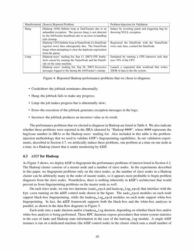
Manifestation [Source] Reported Problem Problem-Injection for Validation

Hang [Hadoop 1036] Infinite loop at TaskTracker due to anunhandled exception. The process hang is not detectedby the JobTracker heartbeats due to an error in handlingtask cleanup.

Induce by reverting patch and triggering bug bythrowing NULL exception.

[Hadoop 1255] Infinite loop at NameNode if a DataNoderegisters twice then subsequently dies. The NameNodehangs when attempting to clear the duplicate registrationfrom the queue.

Registered the DataNode with the NameNodetwice and, then, crashed the DataNode.

Limp [Hadoop users’ mailing list, Sep 13, 2007] CPU bottle-neck caused by running the NameNode and the DataN-ode on the same machine.

Emulated by running a CPU-intensive task thatuses 70% of the CPU.

[Hadoop users’ mailing list, Sep 26, 2007] Excessivemessages logged to file during the JobTracker’s startup.

Launch a sequential disk workload that writes20GB of data to the file system.

Figure 4: Reported Hadoop performance problems that we chose to diagnose.

• Crash/abort–the job/task terminates abnormally;

• Hang–the job/task fails to make any progress;

• Limp–the job makes progress but is abnormally slow;

• Error–the execution of the job/task generates exception messages in the logs;

• Incorrect–the job/task produces an incorrect value as its result.

The performance problems that we elected to diagnose in Hadoop are listed in Table 4. We also indicatewhether these problems were reported in the JIRA (denoted by “Hadoop ####”, where #### represents thebug/issue number in JIRA) or the Hadoop users’ mailing list. Also included in this table is the problem-injection methodology that we used to validate ASDF’s fingerpointing capabilities. In our validation experi-ments, described in Section 4.7, we artificially induce these problems, one problem at a time on one node ata time, in a Hadoop cluster that is under monitoring by ASDF.

4.3 ASDF for Hadoop

As Figure 3 shows, we deploy ASDF to fingerpoint the performance problems of interest listed in Section 4.2.The Hadoop cluster consists of a master node and a number of slave nodes. In the experiments describedin this paper, we fingerpoint problems only on the slave nodes, as the number of slave nodes in a Hadoopcluster can be arbitrarily many in the order of master nodes, so it appears most profitable to begin problemdiagnosis from the slave nodes. Nonetheless, there is nothing inherently in ASDF’s architecture that wouldprevent us from fingerpointing problems on the master node as well.

On each slave node, we run two daemons (sadc_rpcd and hadoop_log_rpcd) that interface with thefpt-core running on the ASDF control node shown in the figure. The sadc_rpcd modules on each nodesupport black-box fingerpointing, while the hadoop_log_rpcd modules on each node support white-boxfingerpointing. In fact, the ASDF framework supports both the black-box and the white-box analyses inparallel, as shown in the data-flow diagrams in Figure 5.

Each node runs a sadc daemon and/or a hadoop_log daemon, depending on whether black-box and/orwhite-box analysis is being performed. These RPC daemons expose procedures that return system statisticsin the case of sadc and Hadoop state information in the case of the hadoop_log module. A single ASDF

instance is run on a dedicated machine (the ASDF control node) in the cluster which runs a small number of

10

Figure 5: The DAG constructed by fpt-core to fingerpoint Hadoop.

11

ASDF modules for each machine, each of which makes requests to the RPC daemons of a particular slavenode.

We decided to collect state data from Hadoop’s logs instead of instrumenting Hadoop itself, in keepingwith our original goal of supporting problem diagnosis in production environments. This has the addedadvantage that we do not need to stay up-to-date with changes to the Hadoop source code and can confineourselves to the format of the Hadoop logs alone.

The hadoop_log parser provides on-demand, lazy parsing of the logs generated by each of the HadoopDataNode and TaskTracker instances to generate counts of event and state occurrences (as defined in Sec-tion 4.4). All information from prior log entries is summarized and stored in compact internal representa-tions for just sufficiently long durations to infer the states in Hadoop. We refer interested readers to [19]for further implementation details. The ASDF hadoop_log collection module exposes the log parser coun-ters as FPT outputs for analysis modules. Again, ONC RPC is used to collect remote statistics from ahadoop_log_rpcd daemon which provides an interface to the log parser library.

4.4 Hadoop: White-Box Log Analysis

We have devised a novel method to extract white-box metrics which characterize Hadoop’s high-level modesof execution (e.g. Map task, Reduce task taking place) from its textual application logs. Instead of text-mining logs to automatically identify features, we construct an a priori view of the relationship betweenHadoop’s mode of execution and its emitted log entries. This a priori view enabled us to produce structurednumerical data, in the form of a numerical vector, about Hadoop’s mode of execution.

Consider each thread of execution in Hadoop as being approximated by a deterministic finite automaton(DFA), with DFA states corresponding to the different modes of execution. Next, we define events to be theentrance and exit of states, from which we derive DFA transitions as a composition of one state-entrance andone state-exit event. Since Hadoop is multi-threaded, its aggregate high-level mode of execution comprisesmultiple DFAs representing the execution modes in simultaneously executing threads. This aggregate modeis represented by a vector of states for each time instance, showing the number of simultaneously executinginstances of each state. A full list of states that characterize the high-level behavior of Hadoop is in [19].

Each entry in a Hadoop log corresponds to one event–a state-entrance or state-exit event, or an “instant”event (a special case which denotes the immediate entrance to and subsequent exit from a state for short-lived processing, e.g. a block deletion in the Hadoop DataNode). Then, we parse the text entries of theHadoop logs to extract events. By maintaining a minimal amount of state across log entries, we then inferthe vector of states at each time instance by counting the number of entrance and exit events for each state(taking care to include counts of short-lived states, for which entrance and exit events, or instant events,occurred within the same time instance). Some important states for the TaskTracker are Map and Reducetasks, while some important states for the DataNode are those for the data-block reads and writes. Details ofthe log parser implementation and architecture are in [19]. We show, in Figure 6, a snippet of a TaskTrackerlog, and the interpretations that we place on the log entries in order to extract the corresponding Hadoopstates, as we have defined them.

We have currently implemented a log-parser library for the logs gathered from the DataNode and theTaskTracker. This library maintains state that has constant memory use in the order of the duration for whichit is run. In addition, we have implemented an RPC daemon that returns a time series of state vectors fromeach running Hadoop slave, and an ASDF module which harvests state vectors from RPC daemons for use indiagnosis.

To fingerpoint using the white-box metrics, we compute the mean of the samples for a white-boxmetric metric over the window for all the nodes (denoted by mean_metrici for node i) and use the meanvalues for peer comparison. One way to do the peer comparison is to compute the difference (calleddi f f _mean_metrici, j) of mean_metrici at node i with mean_metric j at the other nodes. A node i is classified

12

2008-04-15 14:23:15,324 INFO org.apache.hadoop.mapred.TaskTracker: LaunchTaskAction:

task_0001_m_000096_0

2008-04-15 14:23:16,375 INFO org.apache.hadoop.mapred.TaskTracker: LaunchTaskAction:

task_0001_r_000003_0

2008-04-15 14:23:26,755 INFO org.apache.hadoop.mapred.TaskRunner: task_0001_r_000003_0 Copying

task_0001_m_000128_0 output from pc73.emulab.net.

2008-04-15 14:23:31,595 INFO org.apache.hadoop.mapred.TaskRunner: task_0001_r_000003_0 done

copying task_0001_m_000128_0 output from pc73.emulab.net.

Time . . . MapTask ReduceTask . . . ReduceCopy_Remote . . .

2008-04-15 14:23:15 . . . 1 0 . . . 0 . . .2008-04-15 14:23:16 . . . 1 1 . . . 0 . . .

...2008-04-15 14:23:26 . . . 1 1 . . . 1 . . .2008-04-15 14:23:27 . . . 1 1 . . . 1 . . .

...2008-04-15 14:23:31 . . . 1 1 . . . 0 . . .

Figure 6: A snippet from a TaskTracker Hadoop log showing the log entries that trigger StateStartEventsand StateStopEvents for the ReduceCopyTask_Remote states, along with the log entries that trigger theStateStartEvent for the MapTask and ReduceTask states.

as anomalous if di f f _mean_metrici, j for j = 1,2, . . . ,N is greater than a threshold value for more than N2

nodes. This process can be repeated for all the nodes in the system leading to N2 comparison operations. Toreduce the number of comparisons, we use an alternate method: we compute the median of the mean_metrici

for i = 1,2, . . . ,N (i.e., across all the nodes in the system). Denote the median value median_mean_metric.Since more than N

2 nodes are fault-free the median_mean_metric will correctly represent the metric meanfor fault-free nodes. We then compare mean_metrici for each node i with median_mean_metric value andflag a node as anomalous if the difference is more than a threshold value. A node is fingerpointed duringa window if one or more of its white-box metrics show an anomaly. To determine the threshold values fora white-box metric we first compute the standard deviations of the metric for all the slave nodes over thewindow.

We chose the threshold value for all the metrics to be of the form max{1,k× sigmamedian} where kis a constant (for all the metrics) whose value is chosen to minimize the false positive rate over fault-freetraining data (as explained in Section 4.9). The intuition behind the choice of k×σmedian in the threshold isthat if the metric has a large standard deviation over the window then it is likely that the difference in themean value of the metric across the peers will be larger requiring a larger threshold value to reduce falsepositives and vice versa. The reason for choosing the threshold value to be of the form max1,k×σmedian isthat several white-box metrics tend to be constant in several nodes and vary by a small amount (typically 1)in one node. The fact that the white-box metric is a constant over the window for a node implies that thestandard deviation for that metric will be zero for that node. If several nodes have zero standard deviation,the median standard deviation will also turn out to be zero and will cause significant false positives for thenode on which the metric varies by as small as 1.

4.5 Hadoop: Black-Box Analysis

Our hypothesis for fingerpointing slave nodes in the Hadoop system is that we can use peer comparisonacross the slave nodes to localize the specific node with performance problems. The intuition behind thehypothesis is that on average, the slave nodes will be doing similar processing (map tasks or reduce tasks)

13

and as a result the black-box and white-box metrics would have similar behavior across the nodes in faultfree conditions. The black-box and white-box metrics of the slave nodes will behave similarly even if thereare changes in the workload since a workload change may cause more (or fewer) maps or reduces to belaunched on all the slave nodes. However, when there is a fault in one of the slave nodes, the black-box andwhite-box metrics of the faulty node will show significant departure from that of the other (non-faulty) slavenodes. We can therefore use peer comparison of averaged metrics to detect faulty nodes in the system. Ourhypothesis rests on the following two assumptions i) all the slave nodes are homogeneous and ii) more thanhalf of the nodes in the system are fault-free (otherwise, we may end up fingerpointing the non-faulty nodessince their behavior will differ from the faulty nodes).

Our analysis algorithm gathers black-box as well as white-box metrics from all the slave nodes. Wecollect samples of white-box and black-box metric samples from all the nodes over a window of sizewindowSize. For each node we collect one sample of each white-box and black-box metric per secondover the window. Consecutive windows over which the metrics are collected can overlap with each other byan amount equal to windowOverlap.

In our black-box fingerpointer, we first characterize the workload perceived at each node by using allthe black-box metrics from it. We classify the workload perceived at the node by considering the similarityof its metric vector to a pre-determined set of centroid vectors. Its closest centroid vector is then determinedusing the one Nearest Neighbor (1-NN) approach. The pre-determined set of centroid vectors are generatedby using offline k-Means clustering using fault-free training data consisting different workloads (the randomwriter and sort sample applications, and the Nutch web crawler).

Instead of using raw metric values to characterize workloads, we use the logarithm of every metric sam-ple (we used log(x + 1) for a metric value, x to ensure positive values for logarithms). We used logarithmsto reduce the dynamic range of metric samples since many black-box metrics have a large dynamic range.Furthermore, we scaled the resulting logarithmic metric samples by the standard deviation of the logarithmcomputed over the fault-free training data. We use these vectors of scaled logarithmic metric values (denotedby Xi for node i) for comparison against the pre-determined centroid vectors using the 1-NN approach. Theoutcome of the 1-NN is the assignment of a “state” to each Xi (the index of the centroid vector closest toXi).

For each state we determine the number of vectors Xi that were assigned to it over a window of sizewindowSize. This generates, for a node j, a vector (StateVectorj) whose dimensions are equal to the numberof centroids, and whose k-th component represents the number of times the centroid k was associated withXi for that node in the window. The StateVectorj for j = 1,2,3, . . . ,N are used for peer comparison todetect the anomalous nodes. This is done by first computing a component-wise median vector (denoted bymedianStateVector) and then comparing StateVectorj with medianStateVector. We use the L1 distanceof StateVectorj−medianStateVector for j = 1,2,3, . . . ,N and flag a node j as anomalous if the L1 distanceof StateVectorj−medianStateVector is greater than a pre-determined threshold.

4.6 Metrics

False-positive rate. A false positive occurs when ASDF wrongly fingerpoints a node as a culprit whenthere are no faults on that node. Because alarms demand attention, false alarms divert resources that couldotherwise be utilized for dealing with actual faults. We measured the false-positive rates of our analyses ondata traces where no problems were injected; we can be confident that any alarm raised by ASDF in thesetraces are false positives. By tuning the threshold values for each of our analysis modules, we were able toobserve different average false-positive rates on the problem-free traces.

Fingerpointing latency. An online fingerpointing framework should be able to quickly detect problems inthe system. The fingerpointing latency is the amount of time that elapses from the occurrence of a problemto the corresponding alarm identifying the culprit node. It would be relevant to measure the time interval

14

between the first manifestation of the problem and the raising of the corresponding alarm; however, doing soassumes the ability to tell when the fault first manifested. However, the detection of a fault’s manifestationis precisely the problem that we are attempting to solve. We instead measure the time interval between theinjection of the problem by us and the raising of the corresponding alarm.

4.7 Empirical Validation

We performed our experiments on Hadoop version 0.12.4 running on the amd64 version of Debian GNU/Linux4.0. We verified that the computational usage of ASDF would be constant and small compared to the that ofHadoop. We assumed that each node’s primary responsibility was to run Hadoop jobs. Each DataNode andTaskTracker instance ran on its own node. The NameNode and JobTracker instances also ran on their ownnode. We employed a dedicated ASDF control node to run the fpt-core.

Our experiments were conducted on a 38-node dedicated cluster. Each node consists of an AMDOpteron 1220 dual-core CPU with 4GB of memory, Gigabit Ethernet and a dedicated 320GB disk for HDFSstorage.

ASDF is not dependent on a particular hardware configuration, though the relative overhead of ourinstrumentation is dependent on the amount of memory and processing power available. Although ASDF

assumes the use of Linux and /proc, it is hardware-architecture-agnostic. For our white-box analysis, wemake reasonable assumptions about the format of the Hadoop logs, but our Hadoop-log parser was designedso that changes to the log format could be accounted for.

We ran 10 fault-free workloads on a 6-node Hadoop cluster for each of the following workloads

• RandomWriter (4 Maps, where each Map writes 25GB to HDFS)

• Sort (sorts 6GB of data per node from HDFS)

We selected the parameters for the workloads so that each job ran for about 50 minutes on our cluster.

4.8 Performance Impact of ASDF

There are two concerns when considering the performance impact of ASDF. The first is the impact of datacollection on the running Hadoop applications on the fingerpointee nodes, and the second is the cost of theanalysis on the ASDF control node.

For data collection, it is preferred that the RPC daemons have minimal CPU time, memory, and networkbandwidth overheads so as to minimally alter the runtime performance of the monitored system. In contrast,the cost of analysis on the ASDF control node is of a lesser concern since the fpt-core may run on adedicated or otherwise idle cycle server. However, the cost of this analysis is still important as it dictates thesize of the server needed, or alternatively for a given serrver, determines the number of monitored nodes towhich the fingerpointer may scale.

As depicted in Table 1, for our white-box analysis, the hadoop_log_rpcduses, on average, less than0.02% of CPU time on a single core on cluster nodes, and less than 2.4 MB of resident memory. For ourblack-box analysis, the sadc_rpcd uses less than 0.36% of CPU time, and less than 0.77 MB of residentmemory. Thus, the ASDF data collection has negligible impact on application performance.

For simultaneous black-box and white-box analysis, the fpt-coreprocess on the ASDF control nodeuses, on average, less than 0.81% of CPU time on a single core, and less than 5.1 MB of resident memory, tomonitor five nodes. Since the computation cost of the fingerpointing algorithms used in our analysis agentsscales linearly with the number of monitored nodes, we expect to scale to hundreds of monitored nodes byrunning fpt-core on a single cycle server.

The per-node network bandwidths for both the black-box (sadc) and the white-box (hadoop_log) data-collection are listed in Table 2. Establishing a TCP RPC client connection with each monitored Hadoop slave

15

Process % CPU Memory (MB)hadoop_log_rpcd 0.0245 2.36sadc_rpcd 0.3553 0.77fpt-core 0.8063 5.11

Table 1: CPU usage (% CPU time on a single core) and memory usage (RSS) for the data collectionprocesses and the combined black-box & white-box analysis process.

node incurs a static overhead of 6 kB per-node, and each iteration of data collection costs less than 2 kB/s.Thus, the network bandwith cost of monitoring a single node is negligible, and the aggregate bandwith is onthe order of 1 MB/s even when monitoring hundreds of nodes.

RPC Type Static Ovh. (kB) Per-iter BW (kB/s)sadc-udp 0.80 0.74sadc-tcp 1.98 1.22hl-dn-udp 0.87 0.19hl-dn-tcp 2.04 0.31hl-tt-udp 0.87 0.20hl-tt-tcp 2.04 0.32UDP Sum 2.55 1.13TCP Sum 6.06 1.85

Table 2: RPC bandwidth for both UDP and TCP transports for the three ASDF RPC types: sadc, hadoop_log-datanode, hadoop_log-tasktracker. Static overheads include per-node traffic to create/destroy connections,and the per-iteration bandwidth includes per-node traffic for each iteration (one second) of data collection.

4.9 Results

Black-box Offline Analysis. We conducted two sets of experiments. In the first set, we ran three differentHadoop jobs (and different workloads, RandomWriter and sort) without injecting any problems. Black-boxdata was collected by the ASDF for offline analysis. The windowSize parameter was set to 30 samples. Wevaried the threshold value from 0 to 60 for the problem-free traces to assess the false-positive rates, and thenused the threshold value that resulted in a low false-positive rate.

In the second set of experiments, we ran the RandomWriter and sort workloads, but unlike the firstset of experiments, we injected performance problems from Section 4.2 into the runs. Black-box data wasagain collected, and the black-box analysis module was used to fingerpointings problems. The windowSizeparameter was set to 30 samples, and we measured the false-positive rates for a threshold value of 25.

Figure 7 shows the false-positive rates for the different threshold levels. As the threshold is initiallyincreased from 0, false-positive rates drop rapidly. However, beyond a threshold of 20, any further increasesin threshold lead to little improvement in the false-positive rates.

Table 9 shows that our black-box analysis detects most of the problems injected on the RandomWriterand sort workloads, with the exception of the CPU-hog and disk-hog problems on the RandomWriter. Thisis because disk activity in all slave nodes dominate all other activity, so little difference is observed in theblack-box metrics of the peer slave nodes.White-box Offline Analysis. To validate our white-box analysis module, we ran similar sets of experimentsas those for the black-box analysis. We again chose a windowSize of 30 samples. We varied the value of kfrom 0 to 5 for the problem-free traces to assess the false-positive rates, and then used the value of k that

16

−10 0 10 20 30 40 50 60 700

10

20

30

40

50

60

70

80

90

100False Positive Rates of Black Box Analysis Module

Threshold

Fal

se p

ositi

ve r

ate

(%)

Random WriterSort

Figure 7: False-positive rates for black-box analysis.

0 0.5 1 1.5 2 2.5 3 3.5 4 4.5 50

0.05

0.1

0.15

0.2

0.25False Positive Rates of White Box Analysis Module

k

Fal

se p

ositi

ve r

ate

(%)

Random WriterSort

Figure 8: False-positive rates for white-box analysis.

resulted in a low false-positive rate.For the second set of experiments, we induced the performance problems listed in Section 4.2, and ran

the white-box analysis module offline on the data collected during the run. The same windowSize of 30samples was chosen, and k was set to 2.

Figure 8 shows the false-positive rates for the different values of k. False-positive rates are under 0.2%,and we observe little improvement when the value of k is increased beyond 2.

Table 9 shows that we were able to detect the Hadoop problem 1036. However, the resource hogsand Hadoop problem 1255 were not detected. Since Hadoop is unaware of activity outside of itself, thewhite-box analysis module is unable to detect the resource hogs. The culprit node in Hadoop problem 1255crashes, and thus, no further log events are produced, resulting in the white-box module being able to detectthe problem.White- and Black-box Online Analysis. In addition to the above two experiments, we also used our onlinefingerpointing framework with both black- and white-box metrics to successfully fingerpoint process-hangs(Hadoop problem 1036 running the RandomWriter workload) in one of the slave nodes.

The latency for fingerpointing the culprit node was less than 1 minute for the online version of our

17

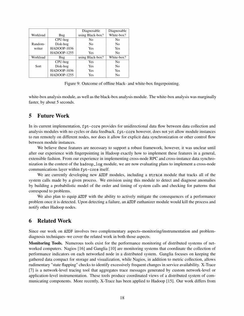
Diagnosable DiagnosableWorkload Bug using Black-box? White-box?

CPU-hog No NoRandom- Disk-hog No No

writer HADOOP-1036 Yes YesHADOOP-1255 Yes No

Workload Bug using Black-box? White-box?CPU-hog Yes No

Sort Disk-hog Yes NoHADOOP-1036 Yes YesHADOOP-1255 Yes No

Figure 9: Outcome of offline black- and white-box fingerpointing.

white-box analysis module, as well as the black-box analysis module. The white-box analysis was marginallyfaster, by about 5 seconds.

5 Future Work

In its current implementation, fpt-core provides for unidirectional data flow between data collection andanalysis modules with no cycles or data feedback. fpt-core however, does not yet allow module instancesto run remotely on different nodes, nor does it allow for explicit data synchronization or other control flowbetween module instances.

We believe these features are necessary to support a robust framework, however, it was unclear untilafter our experience with fingerpointing in Hadoop exactly how to implement these features in a general,extensible fashion. From our experience in implementing cross-node RPC and cross-instance data synchro-nization in the context of the hadoop_log module, we are now evaluating plans to implement a cross-nodecommunications layer within fpt-core itself.

We are currently developing new ASDF modules, including a strace module that tracks all of thesystem calls made by a given process. We envision using this module to detect and diagnose anomaliesby building a probabilistic model of the order and timing of system calls and checking for patterns thatcorrespond to problems.

We also plan to equip ASDF with the ability to actively mitigate the consequences of a performanceproblem once it is detected. Upon detecting a failure, an ASDF euthanizer module would kill the process andnotify other Hadoop nodes.

6 Related Work

Since our work on ASDF involves two complementary aspects–monitoring/instrumentation and problem-diagnosis techniques–we cover the related work in both those aspects.Monitoring Tools. Numerous tools exist for the performance monitoring of distributed systems of net-worked computers. Nagios [16] and Ganglia [10] are monitoring systems that coordinate the collection ofperformance indicators on each networked node in a distributed system. Ganglia focuses on keeping thegathered data compact for storage and visualization, while Nagios, in addition to metric collection, allowsrudimentary "state flapping" checks to identify excessively frequent changes in service availability. X-Trace[7] is a network-level tracing tool that aggregates trace messages generated by custom network-level orapplication-level instrumentation. These tools produce coordinated views of a distributed system of com-municating components. More recently, X-Trace has been applied to Hadoop [15]. Our work differs from

18

these tools by building an automated, online problem-diagnosis framework that can certainly leverage Gan-glia, Nagios and X-Trace output as its data sources, if these data sources are already available in productionenvironments.Application-Log Analysis. Splunk [12], a commercial log-analyzer, treats logs as searchable text indexesand generates views of system anomalies. Our use of application logs, specifically those of Hadoop, differsfrom Splunk by converting logs into numerical data sources that then become immediately comparable withother numerical system metrics.

Cohen et. al. [4] have also examined application logs, but they used feature selection over text-miningof logs to identify co-occurring error messages, and extracted unstructured data from application logs thatlimited the extent to which typical machine learning techniques could be used to synthesize the applicationviews from the application logs and system metrics.Problem-Diagnosis Techniques. Current problem-diagnosis work [1, 13] focuses mostly on collectingtraces of system metrics for offline processing, in order to determine the location and the root-cause ofproblems in distributed systems. While various approaches, such as Magpie [2] and Pinpoint [3], haveexplored the possibility of online implementations (and can arguably be implemented to run in an onlinemanner), they have not been used in an online fashion for live problem localization even as the systemunder diagnosis is executing. Our ASDF framework was intentionally designed for the automated onlinelocalization of problems in a distributed system; this required us to address not just the attendant analyticchallenges, but also the operational issues posed by the requirement of online problem-diagnosis. Cohenet al.’s [5] work continuously builds ensembles of models in an online fashion and attemtps to performdiagnosis online. Our work differs from that of Cohen et al. by building a pluggable architecture, intowhich arbitrary data sources can be fed to synthesize information across nodes. This enables us to utilizeinformation from multiple data sources simultaneously to present a unified system view as well as to supportautomated problem-diagnosis.

In addition, Pinpoint, Magpie, and Cohen et al.’s work rely on large numbers of requests to use aslabeled training data a priori for characterizing the system’s normal behavior via clustering. However,Hadoop has a workload of long-running jobs, with users initiating jobs at a low frequency, rendering thesetechniques unsuitable. Pip [14], which relies on detecting anomalous execution paths from many possibleones, will also have limited effectiveness at diagnosing problems in Hadoop. Execution paths in Hadoop aregenerally uninteresting for problem-diagnosis, as these paths are homogeneous within any given job, andoffer limited opportunities for clustering to infer other types of possible normal paths.

The idea of correlating system behavior across multiple layers of a system is not new. Hauswirth etal’s "vertical profiling" [11] aims to understand the behavior of object-oriented applications by correlatingmetrics collected at various abstraction levels in the system. Vertical profiling was used to diagnose per-formance problems in applications in a debugging context at development time, requiring access to sourcecode while our approach diagnoses performance problems in production systems without using applicationknowledge.

Triage [21] uses a check-point/reexecution framework to diagnose software failures on a single machinein a production environment. They leverage an ensemble of program analysis (white-box) techniques tolocalize the root-cause of problems. ASDF is designed to flexibly integrate both black-box and white-boxdata sources, providing the opportunity to diagnose problems both within the application, and due to externalfactors in the environment. Triage targeted single-host systems whereas ASDF targets distributed systems.

7 Conclusion

In this paper, we described our experience in designing and implementing the ASDF online problem-localizationframework. The architecture is intentionally designed for flexibility in adding or removing multiple, dif-

19

ferent data-sources and multiple, different data-analysis techniques. This flexibility allows us to attach anumber of data-sources for analysis, as needed, and then to detach any specific data-sources if they are nolonger needed.

We also applied this Hadoop, effectively demonstrating that we can localize performance problems (thathave been reported in Apache’s JIRA issue tracker [8]) using both black-box and white-box approaches, fora variety of workloads and even in the face of workload changes. We demonstrate that we can perform onlinefingerpointing in real time, that our framework incurs reasonable overheads and that our false-positive ratesare low.

References

[1] M. K. Aguilera, J. C. Mogul, J. L. Wiener, P. Reynolds, and A. Muthitacharoen. Performance de-bugging for distributed system of black boxes. In ACM Symposium on Operating Systems Principles,pages 74–89, Bolton Landing, NY, October 2003.

[2] P. Barham, A. Donnelly, R. Isaacs, and R. Mortier. Using Magpie for request extraction and workloadmodelling. In USENIX Symposium on Operating Systems Design and Implementation, pages 259–272,San Francisco, CA, December 2004.

[3] M. Y. Chen, E. Kiciman, E. Fratkin, A. Fox, and E. Brewer. Pinpoint: Problem determination in large,dynamic internet services. In IEEE Conference on Dependable Systems and Networks, June 2002.

[4] Ira Cohen. Machine learning for automated diagnosis of distributed systems performance. SF BayACM Data Mining SIG, August 2006.

[5] Ira Cohen, Steve Zhang, Moises Goldszmidt, Julie Symons, Terence Kelly, and Armando Fox. Cap-turing, indexing, clustering, and retrieving system history. pages 105–118. ACM.

[6] J. Dean and S. Ghemawat. MapReduce: Simplified data processing on large clusters. In USENIXSymposium on Operating Systems Design and Implementation, pages 137–150, San Francisco, CA,December 2004.

[7] Rodrigo Fonseca, George Porter, Randy H. Katz, Scott Shenker, and Ion Stoica. X-Trace: A pervasivenetwork tracing framework. In USENIX Symposium on Networked Systems Design and Implementa-tion, Cambridge, MA, April 2007.

[8] The Apache Software Foundation. Apache’s jira issue tracker, 2006. https://issues.apache.org/jira.

[9] The Apache Software Foundation. Hadoop, 2007. http://lucene.apache.org/hadoop.

[10] Ganglia. Ganglia monitoring system, 2007. http://ganglia.info.

[11] M. Hauswirth, A. Diwan, P. Sweeney, and M. Hind. Vertical profiling: Understanding the behav-ior of object-oriented applications. In ACM Conference on Object-Oriented Programming, Systems,Languages, and Applications, pages 251 – 269, Vancouver, BC, Canada, October 2004.

[12] Splunk Inc. Splunk: The it search company, 2005. http://www.splunk.com.

[13] E. Kiciman and A. Fox. Detecting application-level failures in component-based internet services.IEEE Transactions on Neural Networks: Special Issue on Adaptive Learning Systems in Communica-tion Networks, 16(5):1027– 1041, September 2005.

20

[14] E. Kiciman and A. Fox. Detecting application-level failures in component-based internet services. InUSENIX Symposium on Networked Systems Design and Implementation, pages 115– 128, San Jose,CA, May 2006.

[15] Andy Konwinski and Matei Zaharia. Finding the elephant in the data center: Tracing hadoop. Tech-nical Report Unpublished, University of California, Berkeley Electrical Engineering and ComputerScience, May 2008.

[16] Nagios Enterprises LLC. Nagios, 2008. http://www.nagios.org.

[17] Sun Microsystems. The rpcgen programming guide, 2008. http://docs.sun.com/app/docs/

doc/816-1435/rpcgenpguide-24243.

[18] H. Gobioff S. Ghemawat and S. Leung. The google file system. In ACM Symposium on OperatingSystems Principles, pages 29 – 43, Lake George, NY, October 2003.

[19] Jiaqi Tan. RAMS and BlackSheep: Inferring white-box application behavior using black-box tech-niques. Technical Report CMU-PDL-08-103, Carnegie Mellon University Parallel Data Laboratory,May 2008.

[20] BLFS Development Team. System utilities: Sysstat.

[21] Joseph Tucek, Shan Lu, Chengdu Huang, Spiros Xanthos, and Yuanyuan Zhou. Triage: diagnosingproduction run failures at the user’s site. In Symposium on Operating Systems Principles (SOSP),pages 131–144, Stevenson, WA, October 2007.

21