A Rudimentary Knowledge of

Multivariate Analysis

Nobuaki Obata

www.math.is.tohoku.ac.jp/~obata

November 18, 25, December 2, 2016

Contents of Lectures

P. G. Hoel: Introduction to Mathematical Statistics, Wileyor other similar books

Lecture 1. Random Vectors and Multi-Dimensional Distributions[Hoel] Chaps 2-3, 6

Lecture 2. Statistical Inference[Hoel] Chaps 4-5, 8

Lecture 3. Normal Linear Models [Hoel] Chaps 6-7

References

2

Further reading toward generalized linear models

Generalized Linear Models (GLM)1) tracing back to

J. Nelder and R. Wedderburn (1972)2) unifying various other statistical models,

i.e., t-test, 𝜒2-test, linear regression, logistic regression, Poisson regression.

3) based on Least Squares Method and Maximum Likelihood Estimation

[1] A. J. Dobson and A. G. Barnett: An Introduction to Generalized Linear Models,3rd Edition, CRC Press, 2008. [Japanese translation available for 2nd Edition]

[2] P. McCullagh and J. A. Nelder: generalized Linear Models, 2nd Edition,Chapman & Hall, 1989.

3

Lecture 1

Random Vectors and

Multi-Dimensional Distributions

1. Real data vs random variables

Collecting numerical data No 𝑥 𝑦

1 𝑥1 𝑦1

2 𝑥2 𝑦2

⋮ ⋮ ⋮

𝑛 𝑥𝑛 𝑦𝑛

No 𝑥

1 𝑥1

2 𝑥2

⋮ ⋮

𝑛 𝑥𝑛

1 dim. data 2 dim. data

We needmathematical

or statistical model𝑥

𝑋

1 dim. random variable

𝑋, 𝑌

2 dim. random vector

𝑥

𝑦

Population

2. Random variables and distributions

• range of values {𝑎1, 𝑎2, … , 𝑎𝑛, … }

• distribution by point masses

𝑃 𝑋 = 𝑎𝑛 = 𝑝𝑛, 𝑝𝑛≥ 0,

𝑛

𝑝𝑛 = 1

mean value

variance

𝜎2 = 𝜎𝑋2 = 𝐕 𝑋 = 𝐄 𝑋 − 𝑚 2 =

𝑛

𝑎𝑛 − 𝑚 2 𝑝𝑛

𝑚 = 𝑚𝑋 = 𝐄 𝑋 =

𝑛

𝑎𝑛 𝑝𝑛

= 𝐄 𝑋2 − 𝑚2 =

𝑛

𝑎𝑛2 𝑝𝑛 − 𝑚2

6

Discrete case

• range of values 𝐼 ⊂ 𝐑 = −∞,+∞

• distribution by density function

𝑃 𝑎 ≤ 𝑋 ≤ 𝑏 = 𝑎

𝑏

𝑓𝑋 𝑥 𝑑𝑥

mean value

𝑚 = 𝑚𝑋 = 𝐄 𝑋 = −∞

+∞

𝑥𝑓𝑋 𝑥 𝑑𝑥

variance

𝜎2 = 𝜎𝑋2 = 𝐕 𝑋 = 𝐄 𝑋 − 𝑚 2 =

−∞

+∞

𝑥 − 𝑚 2𝑓𝑋 𝑥 𝑑𝑥

= 𝐄 𝑋2 − 𝑚2 = −∞

+∞

𝑥2𝑓𝑋 𝑥 𝑑𝑥 − 𝑚2

𝑓𝑋 𝑥 ≥ 0, −∞

+∞

𝑓𝑋 𝑥 𝑑𝑥 = 1

7

Continuous case

3. Some probability distributions

Discrete distributions mean variance

binomial distribution 𝐵(𝑛,𝑝) 𝑛𝑝 𝑛𝑝 1 − 𝑝

Bernoulli distribution 𝐵(1,𝑝) 𝑝 𝑝 1 − 𝑝

geometric distribution with parameter 𝑝 1/𝑝 1/𝑝2

Poisson distribution with parameter 𝜆 Po(𝜆) 𝜆 𝜆

Continuous distributions mean variance

uniform distribution on [𝑎,𝑏] 𝑎 + 𝑏 /2 𝑏 − 𝑎 2/12

exponential distribution with parameter 𝜆 1/𝜆 1/𝜆2

normal (or Gaussian) distribution 𝑁(𝑚, 𝜎2) 𝑚 𝜎2

chi-square distribution 𝜒2 𝑛 𝑛 2𝑛

F-distribution 𝐹 𝑚, 𝑛 = 𝐹𝑛𝑚 𝑛/ 𝑛 − 2 2𝑛2 𝑚 + 𝑛 − 2

/𝑚 𝑛 − 2 2 𝑛 − 48

Binomial distribution

0

0.05

0.1

0.15

0.2

0.25

0.3

0 1 2 3 4 5 6 7 8 9 10

B(10,1/2)

0

0.05

0.1

0.15

0.2

0.25

0.3

1 2 3 4 5 6 7 8 9 10 11

Po(2.5)

𝑃 𝑋 = 𝑘 =𝑛𝑘

𝑝𝑘 1 − 𝑝 𝑛−𝑘

𝐵 𝑛, 𝑝 Po 𝜆

𝑃 𝑋 = 𝑘 =𝜆𝑘

𝑘!𝑒−𝜆, 𝑘 = 0,1,2,…

Poisson distribution

𝑘 = 0,1,2,… , 𝑛

9

Normal distribution 𝑁(𝑚, 𝜎2)

𝑋 ~ 𝑁(𝑚, 𝜎2) means that

𝑃 𝑎 ≤ 𝑋 ≤ 𝑏 = 𝑎

𝑏

𝑓 𝑥 𝑑𝑥

𝑓 𝑥 =1

2𝜋𝜎2exp −

𝑥 − 𝑚 2

2𝜎2

density function

𝑚 = 𝑚𝑋 = 𝐄 𝑋 = −∞

+∞

𝑥𝑓 𝑥 𝑑𝑥

𝜎2 = 𝜎𝑋𝑋 = 𝜎𝑋2 = 𝐕 𝑋 = 𝐄 𝑋 − 𝑚 2 =

−∞

+∞

𝑥 − 𝑚 2𝑓 𝑥 𝑑𝑥

mean value:

variance:10

11

Standard normal distribution 𝑁(0,1)

𝑓 𝑥 =1

2𝜋exp −

1

2𝑥2

𝜎2 = 1normal distribution with and 𝑚 = 0

𝑁(0,1) :

In general, the normalization of 𝑋 is defined by

𝑋 =𝑋 − 𝑚

𝜎where 𝑚 = 𝐄 𝑋 and 𝜎2= 𝐕[𝑋].

Then we have 𝐄 𝑋 = 0 and 𝐕 𝑋 = 1.

THEOREM

(1) If 𝑋 ~ 𝑁(𝑚, 𝜎2), then 𝑋 =𝑋−𝑚

𝜎~ 𝑁(0,1).

(2) If 𝑍 ~ 𝑁(0,1), then 𝑎𝑍 + 𝑏 ~ 𝑁(𝑏, 𝑎2 ).

12

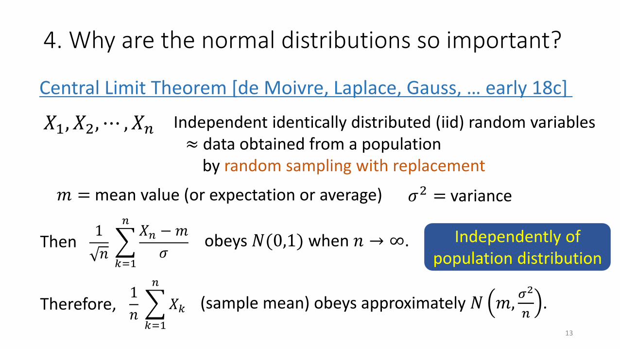
4. Why are the normal distributions so important?

13

Central Limit Theorem [de Moivre, Laplace, Gauss, … early 18c]

Independent identically distributed (iid) random variables≈ data obtained from a population

by random sampling with replacement

𝑋1, 𝑋2, ⋯ , 𝑋𝑛

𝑚 = mean value (or expectation or average) 𝜎2 = variance

1

𝑛

𝑘=1

𝑛𝑋𝑛 − 𝑚

𝜎obeys 𝑁(0,1) when 𝑛 → ∞.Then

Therefore, 1

𝑛

𝑘=1

𝑛

𝑋𝑘 (sample mean) obeys approximately 𝑁 𝑚,𝜎2

𝑛.

Independently of population distribution

5. Random vectors and joint probability distributions

Their probability distribution is described by the joint distribution.

(1) For discrete random variables: 𝑃 𝑋1 = 𝑎1, 𝑋2 = 𝑎2, ⋯ , 𝑋𝑛 = 𝑎𝑛

(2) For continuous random variables we use the joint density function:

𝑃 𝑋1 ≤ 𝑎1, 𝑋2 ≤ 𝑎2, ⋯ , 𝑋𝑛 ≤ 𝑎𝑛 = −∞

𝑎1

−∞

𝑎2

⋯ −∞

𝑎𝑛

𝑓 𝑥1, 𝑥2, ⋯ , 𝑥𝑛 𝑑𝑥1𝑑𝑥2 ⋯𝑑𝑥𝑛

a random vector

𝑿 =

𝑋1

𝑋2

⋮𝑋𝑛

or 𝑿 = 𝑋1 𝑋2 ⋯ 𝑋𝑛𝑇

14

a finite set of random variables

𝑋1, 𝑋2, ⋯ , 𝑋𝑛

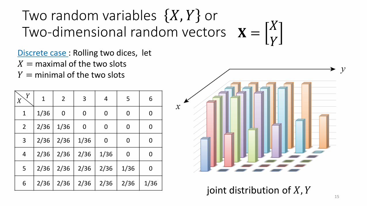
Two random variables 𝑋, 𝑌 or Two-dimensional random vectors 𝐗 =

𝑋𝑌

Discrete case : Rolling two dices, let𝑋 = maximal of the two slots𝑌 = minimal of the two slots

1 2 3 4 5 6

1 1/36 0 0 0 0 0

2 2/36 1/36 0 0 0 0

3 2/36 2/36 1/36 0 0 0

4 2/36 2/36 2/36 1/36 0 0

5 2/36 2/36 2/36 2/36 1/36 0

6 2/36 2/36 2/36 2/36 2/36 1/36

𝑋𝑌

joint distribution of 𝑋, 𝑌15

Two-dimensional joint density function

𝑓 𝑥, 𝑦 is a density function if

Continuous case: We use joint density function

𝑃 𝑋, 𝑌 ∈ 𝐷 = 𝐷

𝑓𝑋𝑌 𝑥, 𝑦 𝑑𝑥𝑑𝑦

𝑓 𝑥, 𝑦 ≥ 0

−∞

+∞

−∞

+∞

𝑓 𝑥, 𝑦 𝑑𝑥𝑑𝑦 = 1

(i)

(ii)

16

𝑏1 ⋯ 𝑏𝑗 ⋯ 𝑏𝑛 sum

𝑎1 𝑃 𝑋 = 𝑎1

⋮

𝑎𝑖 𝑝𝑖1 ⋯ 𝑝𝑖𝑗 ⋯ 𝑝𝑖𝑛 𝑃 𝑋 = 𝑎𝑖

⋮

𝑎𝑚 𝑃 𝑋 = 𝑎𝑚

sum 1

6. Marginal distribution and conditional distribution

𝑃 𝑋 = 𝑎𝑖 =

𝑗

𝑃 𝑋 = 𝑎𝑖 , 𝑌 = 𝑏𝑗

𝑃 𝑋 = 𝑎𝑖 | 𝑌 = 𝑏𝑗 =𝑃 𝑋 = 𝑎𝑖 , 𝑌 = 𝑏𝑗

𝑃 𝑌 = 𝑏𝑗

𝑋𝑌

Marginal distribution of 𝑋Marginal distribution of 𝑌

𝑓𝑋 𝑥 = −∞

+∞

𝑓𝑋𝑌 𝑥, 𝑦 𝑑𝑦

𝑓𝑋|𝑌 𝑥|𝑦 =𝑓𝑋𝑌 𝑥, 𝑦

𝑓𝑌(𝑦)

Discrete case

Continuous case

17

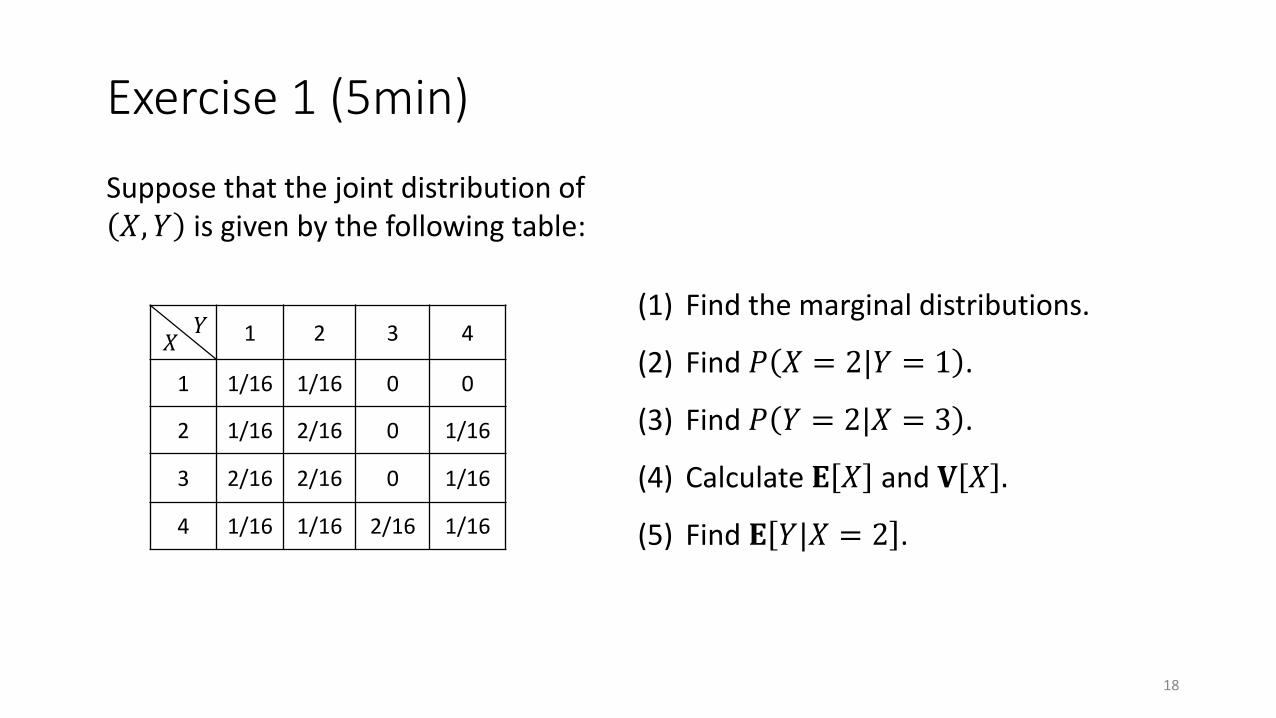
Exercise 1 (5min)

Suppose that the joint distribution of 𝑋, 𝑌 is given by the following table:

1 2 3 4

1 1/16 1/16 0 0

2 1/16 2/16 0 1/16

3 2/16 2/16 0 1/16

4 1/16 1/16 2/16 1/16

𝑋𝑌

(1) Find the marginal distributions.

(2) Find 𝑃 𝑋 = 2|𝑌 = 1 .

(3) Find 𝑃 𝑌 = 2|𝑋 = 3 .

(4) Calculate 𝐄 𝑋 and 𝐕 𝑋 .

(5) Find 𝐄 𝑌|𝑋 = 2 .

18

7. Covariance and correlation coefficient

Relation to the normalized random variables:

𝜌 𝑋, 𝑌 = 𝐄𝑋 − 𝐄 𝑋

𝑉 𝑋∙𝑌 − 𝐄 𝑌

𝑉 𝑌= 𝐸 𝑋 𝑌 = 𝐂𝐨𝐯 𝑋, 𝑌 = 𝜌 𝑋, 𝑌

𝜌 𝑋, 𝑌 =𝐂𝐨𝐯 𝑋, 𝑌

𝑉 𝑋 𝑉 𝑌=

𝜎𝑋𝑌

𝜎𝑋𝜎𝑌

𝐂𝐨𝐯 𝑋, 𝑌 = 𝐄 𝑋 − 𝐄 𝑋 𝑌 − 𝐄 𝑌

= 𝐄 𝑋𝑌 − 𝐄 𝑋 𝐄 𝑌

19

𝑚𝑋 = 𝐄 𝑋

Exercise 2 (10min)

Suppose that the joint distribution of 𝑋, 𝑌 is given by the following table:

1 2 3 4

1 1/16 1/16 0 0

2 1/16 2/16 0 1/16

3 2/16 2/16 0 1/16

4 1/16 1/16 2/16 1/16

𝑋𝑌 (1) Calculate 𝐂𝐨𝐯 𝑋, 𝑌 .

(2) Calculate ρ 𝑋, 𝑌 .

20

7. Independent random variables

A set of random variables 𝑋1, 𝑋2, ⋯ , 𝑋𝑛 is called independent if

If 𝑋1, 𝑋2, ⋯ , 𝑋𝑛 are discrete random variables, (*) is equivalent to

𝑃 𝑋1 = 𝑎1, 𝑋2 = 𝑎2, ⋯ , 𝑋𝑛 = 𝑎𝑛 =

𝑘=1

𝑛

𝑃 𝑋𝑘 = 𝑎𝑘

If 𝑋1, 𝑋2, ⋯ , 𝑋𝑛 are continuous random variables, (*) is equivalent to

𝑃 𝑋1 ≤ 𝑎1, 𝑋2 ≤ 𝑎2, ⋯ , 𝑋𝑛 ≤ 𝑎𝑛 =

𝑘=1

𝑛

𝑃 𝑋𝑘 ≤ 𝑎𝑘(*)

𝑓𝑋1,𝑋2,⋯,𝑋𝑛𝑥1, 𝑥2, ⋯ , 𝑥𝑛 =

𝑘=1

𝑛

𝑓𝑋𝑘𝑥𝑘

21

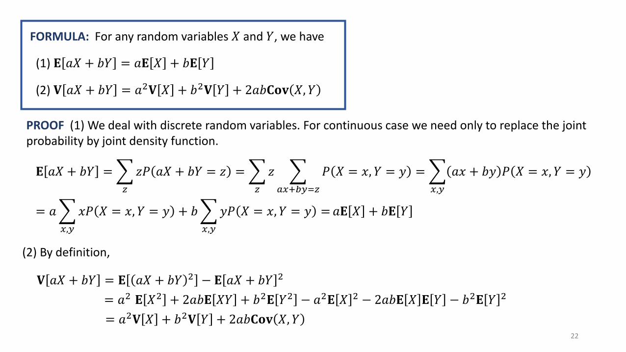
PROOF (1) We deal with discrete random variables. For continuous case we need only to replace the joint probability by joint density function.

𝐄 𝑎𝑋 + 𝑏𝑌 =

𝑧

𝑧𝑃 𝑎𝑋 + 𝑏𝑌 = 𝑧 =

𝑧

𝑧

𝑎𝑥+𝑏𝑦=𝑧

𝑃 𝑋 = 𝑥, 𝑌 = 𝑦 =

𝑥,𝑦

𝑎𝑥 + 𝑏𝑦 𝑃 𝑋 = 𝑥, 𝑌 = 𝑦

= 𝑎

𝑥,𝑦

𝑥𝑃 𝑋 = 𝑥, 𝑌 = 𝑦 + 𝑏

𝑥,𝑦

𝑦𝑃 𝑋 = 𝑥, 𝑌 = 𝑦 =𝑎𝐄 𝑋 + 𝑏𝐄 𝑌

(2) By definition,

𝐕 𝑎𝑋 + 𝑏𝑌 = 𝐄 𝑎𝑋 + 𝑏𝑌 2 − 𝐄 𝑎𝑋 + 𝑏𝑌 2

= 𝑎2 𝐄 𝑋2 + 2𝑎𝑏𝐄 𝑋𝑌 + 𝑏2𝐄 𝑌2 − 𝑎2𝐄 𝑋 2 − 2𝑎𝑏𝐄 𝑋 𝐄 𝑌 − 𝑏2𝐄 𝑌 2

= 𝑎2𝐕 𝑋 + 𝑏2𝐕 𝑌 + 2𝑎𝑏𝐂𝐨𝐯 𝑋, 𝑌

(2) 𝐕 𝑎𝑋 + 𝑏𝑌 = 𝑎2𝐕 𝑋 + 𝑏2𝐕 𝑌 + 2𝑎𝑏𝐂𝐨𝐯 𝑋, 𝑌

(1) 𝐄 𝑎𝑋 + 𝑏𝑌 = 𝑎𝐄 𝑋 + 𝑏𝐄 𝑌

FORMULA: For any random variables 𝑋 and 𝑌, we have

22

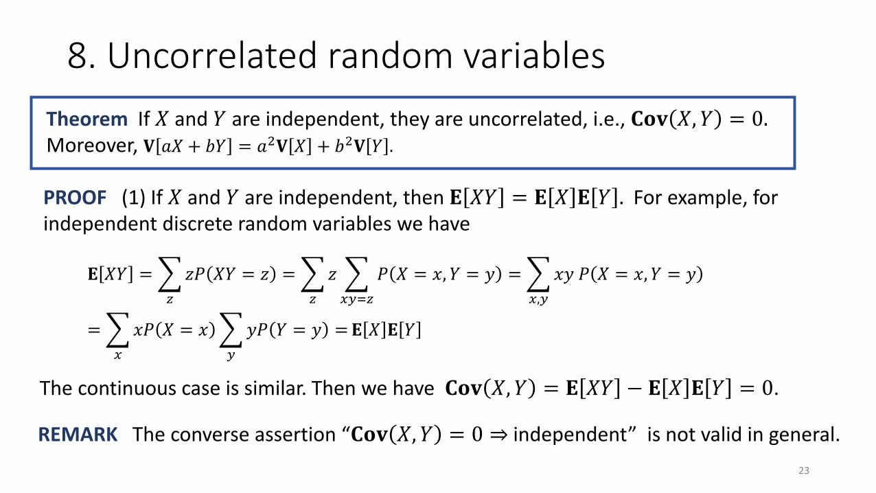
8. Uncorrelated random variables

Theorem If 𝑋 and 𝑌 are independent, they are uncorrelated, i.e., 𝐂𝐨𝐯 𝑋, 𝑌 = 0.Moreover, 𝐕 𝑎𝑋 + 𝑏𝑌 = 𝑎2𝐕 𝑋 + 𝑏2𝐕 𝑌 .

The continuous case is similar. Then we have 𝐂𝐨𝐯 𝑋, 𝑌 = 𝐄 𝑋𝑌 − 𝐄 𝑋 𝐄 𝑌 = 0.

PROOF (1) If 𝑋 and 𝑌 are independent, then 𝐄 𝑋𝑌 = 𝐄 𝑋 𝐄 𝑌 . For example, forindependent discrete random variables we have

23

REMARK The converse assertion “𝐂𝐨𝐯 𝑋, 𝑌 = 0 ⇒ independent” is not valid in general.

𝐄 𝑋𝑌 =

𝑧

𝑧𝑃 𝑋𝑌 = 𝑧 =

𝑧

𝑧

𝑥𝑦=𝑧

𝑃 𝑋 = 𝑥, 𝑌 = 𝑦 =

𝑥,𝑦

𝑥𝑦 𝑃 𝑋 = 𝑥, 𝑌 = 𝑦

=

𝑥

𝑥𝑃 𝑋 = 𝑥

𝑦

𝑦𝑃 𝑌 = 𝑦 =𝐄 𝑋 𝐄 𝑌

9. Two-dimensional normal distribution

𝑓 𝑥, 𝑦 = 𝐾 exp − 𝑎𝑥2 + 2𝑏𝑥𝑦 + 𝑐𝑦2 + 𝛼𝑥 + 𝛽𝑦 + 𝛾

𝑓 𝑥 =1

2𝜋𝜎2exp −

𝑥 − 𝑚 2

2𝜎2

The essential part of 𝑓 𝑥 is exp −𝑎𝑥2 , where the quadratic function ℎ 𝑥 = 𝑎𝑥2 is“positive.”

If ℎ 𝑥 = 𝑎𝑥2 + 2𝑏𝑥𝑦 + 𝑐𝑦2 is ``positive,” we have a density function of the form:

2-dimensional case

1-dimensional case

24

Quadratic forms in vector notation

𝑓 𝑥, 𝑦 = 𝑎𝑥2 + 2𝑏𝑥𝑦 + 𝑐𝑦2 = 𝒙, 𝐴𝒙

The canonical inner product is defined by

𝒙1, 𝒙2 =𝑥1

𝑦1,𝑥2

𝑦2= 𝑥1𝑥2 + 𝑦1𝑦2

𝑓 𝑥, 𝑦 = 𝑎𝑥2 + 2𝑏𝑥𝑦 + 𝑐𝑦2 where 𝑎, 𝑏, 𝑐 ≠ 0,0,0

Setting 𝒙 =𝑥𝑦 and 𝐴 =

𝑎 𝑏𝑏 𝑐

, we obtain

We then see easily that

𝑎𝑥2 + 2𝑏𝑥𝑦 + 𝑐𝑦2 =𝑥𝑦 ,

𝑎 𝑏𝑏 𝑐

𝑥𝑦

In general, given a symmetric matrix 𝐴 thequadratic form is defined by

𝑓 𝒙 = 𝒙, 𝐴𝒙

A quadratic form is called positive (or positive definite) if

𝒙, 𝐴𝒙 > 0 for all 𝒙 with 𝒙 ≠ 𝟎.In this case the matrix 𝐴 is called positivedefinite. This condition is equivalent to thatall the eigenvalues of matrix 𝐴 is positive.

25

Two-dimensional normal distribution 𝑁 𝒎, Σ

𝑚𝑥 = −∞

+∞

−∞

+∞

𝑥𝑓 𝑥, 𝑦 𝑑𝑥𝑑𝑦 = 𝑎

𝜎𝑥2 =

−∞

+∞

−∞

+∞

𝑥 − 𝑎 2𝑓 𝑥, 𝑦 𝑑𝑥𝑑𝑦 =𝜎11

𝜎𝑥𝑦 = −∞

+∞

−∞

+∞

𝑥 − 𝑎 𝑦 − 𝑏 𝑓 𝑥, 𝑦 𝑑𝑥𝑑𝑦 = 𝜎12 = 𝜎21

For a vector 𝒎 =𝑎𝑏

and a positive definite matrix Σ =𝜎11 𝜎12

𝜎21 𝜎22𝜎12 = 𝜎21 ,

becomes a density function (i.e., ). Moreover, by direct calculation we obtain −∞

+∞

−∞

+∞

𝑓 𝑥, 𝑦 𝑑𝑥𝑑𝑦 = 1

𝑚𝑦 = −∞

+∞

−∞

+∞

𝑦𝑓 𝑥, 𝑦 𝑑𝑥𝑑𝑦 = 𝑏

𝜎𝑦2 =

−∞

+∞

−∞

+∞

𝑦 − 𝑏 2𝑓 𝑥, 𝑦 𝑑𝑥𝑑𝑦 =𝜎22

Thus, 𝒎 is the mean vector and Σ is the variance-covariance matrix.

𝑓 𝑥, 𝑦 = 𝑓 𝒙 =1

2𝜋 2 Σexp −

1

2𝒙 − 𝒎 , Σ−1 𝒙 − 𝒎𝑁 𝒎, Σ : Σ = det Σ

26

PROOF. Recall first that

Then

𝑓 𝑥, 𝑦 =1

2𝜋 2 Σexp −

1

2𝒙 − 𝒎 , Σ−1 𝒙 − 𝒎

=1

2𝜋 2𝜎𝑥𝑥𝜎𝑦𝑦

exp −1

2𝜎𝑥𝑥

−1 𝑥 − 𝑚𝑋2 + 𝜎𝑦𝑦

−1 𝑦 − 𝑚 2

=1

2𝜋𝜎𝑥2exp −

𝑥 − 𝑚𝑋2

2𝜎𝑥2 ×

1

2𝜋𝜎𝑦2

exp −𝑦 − 𝑚𝑌

2

2𝜎𝑦2

= 𝑓𝑋 𝑥 𝑓𝑌 𝑦

𝒙 − 𝒎 , Σ−1 𝒙 − 𝒎

=𝑥 − 𝑚𝑋

𝑦 − 𝑚𝑌,𝜎𝑥𝑥

−1 0

0 𝜎𝑦𝑦−1

𝑥 − 𝑚𝑋

𝑦 − 𝑚𝑌

= 𝜎𝑥𝑥−1 𝑥 − 𝑚𝑋

2 + 𝜎𝑥𝑥−1 𝑥 − 𝑚𝑋

2

𝜎𝑥𝑥 = 𝜎𝑥2 , 𝜎𝑦𝑦= 𝜎𝑦

2,

𝜎𝑥𝑦 = 𝜎𝑦𝑥 = 𝐂𝐨𝐯 𝑋, 𝑌

Σ = 𝜎𝑥𝑥𝜎𝑦𝑦

Since the joint density function is factorized, 𝑋 and 𝑌 are independent.

Σ =𝜎𝑥𝑥 𝜎𝑥𝑦

𝜎𝑦𝑥 𝜎𝑦𝑦=

𝜎𝑥𝑥 00 𝜎𝑦𝑦

27

THEOREM: Assume that a random vector 𝑋, 𝑌 obeys 2-dimensional normal distribution 𝑁 𝒎, Σ . Then, 𝐂𝐨𝐯 𝑋, 𝑌 = 0 ⇔ 𝑋 and 𝑌 are independent.

27

During my lectures you will be given 10 Problems.

Choose 4 problems at your own taste and write up a short report.

Submission deadline: December 9 (Fri).

Manner of submission: (a) directly hand to Prof Obata

or (b) send in PDF by e-mail to obata@math.is.tohoku.ac.jp

or (c) hand to Prof Nakazawa during the lecture on December 9 (Fri).

Submission of reports for evaluation

28

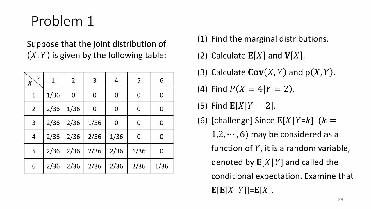
Problem 1

Suppose that the joint distribution of 𝑋, 𝑌 is given by the following table:

1 2 3 4 5 6

1 1/36 0 0 0 0 0

2 2/36 1/36 0 0 0 0

3 2/36 2/36 1/36 0 0 0

4 2/36 2/36 2/36 1/36 0 0

5 2/36 2/36 2/36 2/36 1/36 0

6 2/36 2/36 2/36 2/36 2/36 1/36

𝑋𝑌

(1) Find the marginal distributions.

(2) Calculate 𝐄 𝑋 and 𝐕 𝑋 .

(3) Calculate 𝐂𝐨𝐯 𝑋, 𝑌 and ρ 𝑋, 𝑌 .

(4) Find 𝑃 𝑋 = 4|𝑌 = 2 .

(5) Find 𝐄 𝑋|𝑌 = 2 .

(6) [challenge] Since 𝐄[𝑋|𝑌=𝑘] (𝑘 =

1,2,⋯ , 6) may be considered as a

function of 𝑌, it is a random variable,

denoted by 𝐄[𝑋|𝑌] and called the

conditional expectation. Examine that

𝐄[𝐄[𝑋|𝑌]]=𝐄[𝑋].29

Problem 2

Four cards are drawn from a deck (of 52 cards). Let 𝑋 be the number of acesand 𝑌 the number of kings that show.

(1) Show the joint distribution of 𝑋, 𝑌 , and marginal distributions of 𝑋 and 𝑌.

(2) Find the mean values 𝐄 𝑋 and 𝐄 𝑌 .

(3) Find the variances 𝐕 𝑋 and 𝐕 𝑌 .

(4) Find the covariance 𝐂𝐨𝐯 𝑋, 𝑌 and correlation coefficient 𝜌 𝑋, 𝑌 .

30

Problem 3

Let 𝑋~𝑁 𝑚1, 𝜎12 and 𝑌~𝑁 𝑚2, 𝜎2

2 , and assume that 𝑋 and 𝑌are independent.

(1) Write down the joint density function 𝑓𝑋𝑌 𝑥, 𝑦 .

(2) Find the conditional density function 𝑓𝑌|𝑋 𝑦|𝑥 .

(3) Calculate 𝐄 𝑌|𝑋 = 𝑥

Let 𝑋, 𝑌 be a random vector obeying 2-dimensional normal distribution 𝑁 𝒎, Σ .

Assume that

(1) Write explicitly the joint density function 𝑓𝑋𝑌 𝑥, 𝑦 .

(2) Find the conditional density function 𝑓𝑌|𝑋 𝑦|𝑥 .

Problem 4

𝐄 𝑋 = 2, 𝐄 𝑌 = 3, 𝐕 𝑋 = 1, 𝐕 𝑌 = 2, 𝜚 𝑋, 𝑌 =1

2

32

Solution to Exercise 1

1 2 3 4

1 1/16 1/16 0 0 2/16

2 1/16 2/16 0 1/16 4/16

3 2/16 2/16 0 1/16 5/16

4 1/16 1/16 2/16 1/16 5/16

5/16 6/16 2/16 3/16 1

𝑋𝑌

33𝑃 𝑋 = 2|𝑌 = 1 =

𝑃 𝑋 = 2, 𝑌 = 1

𝑃 𝑌 = 1=

1/16

5/16=

1

5

𝑃 𝑌 = 2|𝑋 = 3 =𝑃 𝑌 = 2, 𝑋 = 3

𝑃 𝑋 = 3=

2/16

5/16=

2

5

𝐄 𝑋 = 12

16+ 2

4

16+ 3

5

16+ 4

5

16=

45

16

𝐄 𝑋2 = 122

16+ 22

4

16+ 32

5

16+ 42

5

16=

143

16

(2)

(3)

(4)

𝐕 𝑋 = 𝐄 𝑋2 − 𝐄 𝑋 2 =143

16−

45

16

2

=263

256

𝐄 𝑌|𝑋 = 2 = 11

4+ 2

2

4+ 4

1

4=

9

4(5)

Solution to Exercise 2

34

1 2 3 4

1 1/16 1/16 0 0 2/16

2 1/16 2/16 0 1/16 4/16

3 2/16 2/16 0 1/16 5/16

4 1/16 1/16 2/16 1/16 5/16

5/16 6/16 2/16 3/16 1

𝑋𝑌

𝐄 𝑌 = 15

16+ 2

6

16+ 3

2

16+ 4

3

16=

35

16

𝐄 𝑌2 = 125

16+ 22

6

16+ 32

2

16+ 42

3

16=

95

16

𝐕 𝑌 = 𝐄 𝑌2 − 𝐄 𝑌 2 =95

16−

35

16

2

=295

256

𝐄 𝑋𝑌 = 1 ∙ 11

16+ 1 ∙ 2

1

16+ 1 ∙ 3 ∙ 0 + ⋯ =

103

16

𝐂𝐨𝐯 𝑋, 𝑌 = 𝐄 𝑋𝑌 − 𝐄 𝑋 𝐄 𝑌

ρ 𝑋, 𝑌 =𝐂𝐨𝐯 𝑋, 𝑌

𝑉 𝑋 𝑉 𝑌=

73

263 ∙ 295= 0.26

=103

16−

45

16

35

16=

73

256