The Pennsylvania State University

The Graduate School

John and Willie Leone Family Department of Energy and Mineral Engineering

A ROBUST LINEAR-PRESSURE ANALOG FOR THE

ANALYSIS OF NATURAL GAS TRANSPORTATION NETWORKS

A Thesis in

Energy and Mineral Engineering

by

Chew Yeong Leong

© 2012 Chew Yeong Leong

Submitted in Partial Fulfillment

of the Requirements

for the Degree of

Master of Science

May 2012

ii

The thesis of Chew Yeong Leong was reviewed and approved* by the following:

Luis F. Ayala H.

Associate Professor of Petroleum and Natural Gas Engineering

Thesis Advisor

Michael Adewumi

Vice Provost for Global Programs

Professor of Petroleum and Natural Gas Engineering

R. Larry Grayson

Professor of Energy and Mineral Engineering;

George H., Jr., and Anne B. Deike Chair in Mining Engineering;

Graduate Program Officer of Energy and Mineral Engineering;

Undergraduate Program Officer of Mining Engineering

*Signatures are on file in the Graduate School

iii

ABSTRACT

Reliable analysis of transportation networks is crucial for design and planning purposes.

A pipeline network system could range from a simple to very sophisticated and complex

arrangement: from a single pipe transporting fluid from a place to another or elaborated

as an interconnected set of fluid networks for intra-state or international transportation.

As the complexity of the network system grows, the solution for the network model

complicates further. For a natural gas network system, the resulting set of fluid flow

governing equations is highly non-linear. In such situations, the customary method

employed for the solution of a set of non-linear equations is the multivariable Newton-

Raphson method despite its potentially negative drawbacks. Newton-Raphson solution

protocols demand a good initialization (i.e., a good initial “guess” of the actual solution)

for satisfactory performance because convergence is only guaranteed to occur within a

potentially narrow neighborhood around the solution vector. This prerequisite can

become fairly restrictive for the solution of large gas network systems, where estimations

of “good” initial gas load and nodal values across the domain can defy intuition. In

addition, some Newton-Raphson formulations require pre-defining flow loops within a

network system prior to attempting a solution, which proves to be a challenging task in an

extensive network. An alternate, simple yet elegant method to address the

aforementioned problems is proposed. The proposed solution methodology retains most

advantages of the Newton-nodal method while removing the need for initial guesses and

eliminating the need for expensive Jacobian formulations and associated derivative

calculations. The resulting linear-pressure analog model is robust, reliable and its

iv

execution and convergence is independent of user-defined initial guesses for nodal

pressures and flow rates. This allows the simulation study of a steady-state gas network

system to be efficiently and straight-forwardly conducted.

v

Table of Contents

LIST OF FIGURES ............................................................................................................ vii

LIST OF TABLES ................................................................................................................ x

LIST OF SYMBOLS ........................................................................................................... xi

ACKNOWLEDGEMENTS ................................................................................................ xv

CHAPTER 1 INTRODUCTION .......................................................................................... 1

CHAPTER 2 LITERATURE REVIEW ............................................................................... 6

CHAPTER 3 NETWORK MODEL ANALYSIS .............................................................. 11

3.1 Pipe Flow Network Equation .................................................................................... 12

3.1.1 Derivation of Pipe Flow Equation for Single-Phase Flow ................................. 13

3.2 Compressor Network Equation ................................................................................. 16

3.2.1 Derivation of Compressor Equation for Single-Phase Flow .............................. 17

3.3 Wellhead Network Equation ..................................................................................... 20

3.4 Newton-Based Gas Network Model ......................................................................... 21

3.4.1 Nodal-loop or q-formulation .............................................................................. 21

3.4.2 Loop or ∆q-formulation ...................................................................................... 23

3.4.3 Nodal or p-formulation ....................................................................................... 24

CHAPTER 4 THE LINEAR PRESSURE ANALOG MODEL ........................................ 26

4.1 Linear Analog Model ................................................................................................ 26

4.1.1 Extension to Networks with Inclined-Pipes ....................................................... 34

4.1.2 Extension to Networks with Compressors .......................................................... 36

4.1.3 Extension to Networks with Wellheads .............................................................. 37

CHAPTER 5 RESULTS AND DISCUSSIONS................................................................. 41

5.1 Case Study 1: Horizontal Pipe Network System ....................................................... 41

5.2 Case Study 2: Inclined Pipe Network System ........................................................... 48

5.3 Case Study 3: Network System with Compression ................................................... 55

5.4 Case Study 4: Network System with Wellheads ....................................................... 62

5.5 Case Study 5: Mexico Valley Field Case .................................................................. 70

CHAPTER 6 CONCLUDING REMARKS........................................................................ 81

vi

BIBLIOGRAPHY ............................................................................................................... 84

APPENDIX ......................................................................................................................... 87

A1 – Input Data for Case Study ...................................................................................... 87

A2 – Linear-Analog Algorithm ....................................................................................... 93

vii

LIST OF FIGURES

Figure 1.1 A pipeline network schematic

Figure 4.1 Derivation of Linear-Pressure Analog Conductivity

Figure 4.2 Analog-pipe conductivity transform (Tij) as a function of pipe pressure

ratio (rij)

Figure 4.3 Flow Chart for Linear-Analog Implementation

Figure 4.4 Analog-well conductivity transform (Tw) as a function of well pressure

ratio (rw) (Pshut = 100 psia)

Figure 5.1.1 Analog-pipe conductivity transform improvement ratio (Tk+1/Tk) vs. no. of

iterations (k) – Case Study 1

Figure 5.1.2 Pressure ratio (rij) vs. no. of iterations (k) – Case Study 1

Figure 5.1.3 Analog-pipe conductivity transform (Tij) vs. pressure ratio (rij) – Case

Study 1

Figure 5.1.4 Nodal pressures (pi) vs. no. of iterations (k) – Case Study 1

Figure 5.1.5 Pipe flow rate (qGij) vs. no. of iterations (k) – Case Study 1

Figure 5.1.6 Fully-converged natural gas network distribution scenario – Case Study 1

Figure 5.2 Node Elevations for Case Study 2

Figure 5.2.1 Analog pipe conductivity transform improvement ratio (Tk+1/Tk) vs. no. of

iterations (k) – Case Study 2

Figure 5.2.2 Pressure ratio (rij) vs. no. of iterations (k) – Case Study 2

Figure 5.2.3 Analog conductivity transform (Tij) vs. pressure ratio (rij) – Case Study 2

Figure 5.2.4 Nodal pressures (pi) vs. no. of iterations (k) – Case Study 2

Figure 5.2.5 Pipe flow rate (qGij) vs. no. of iterations (k) – Case Study 2

viii

Figure 5.2.6 Fully-converged natural gas network distribution – Case Study 2

Figure 5.3 Network Topology of Case Study 3

Figure 5.3.1 Analog pipe conductivity transform improvement ratio (Tk+1/Tk) vs. no. of

iterations (k) – Case Study 3

Figure 5.3.2 Pressure ratio (rij) vs. no. of iterations (k) – Case Study 3

Figure 5.3.3 Analog conductivity transform (Tij) vs. pressure ratio (rij) – Case Study 3

Figure 5.3.4 Nodal pressures (pi) vs. no. of iterations (k) – Case Study 3

Figure 5.3.5: Pipe flow rate (qGij) vs. no. of iterations (k) – Case Study 3

Figure 5.3.6: Fully-converged natural gas network distribution – Case Study 3

Figure 5.4 Network Topology of Case Study 4

Figure 5.4.1 Analog pipe conductivity transform improvement ratio (Tk+1/Tk) vs. no. of

iterations (k) – Case Study 4

Figure 5.4.2 Pressure ratio (rij) vs. no. of iterations (k) – Case Study 4

Figure 5.4.3 Analog conductivity transform (Tij) vs. pressure ratio (rij) – Case Study 4

Figure 5.4.4 Nodal pressures (pi) vs. no. of iterations (k) – Case Study 4

Figure 5.4.5 Pipe flow rate (qGij) vs. no. of iterations (k) – Case Study 4

Figure 5.4.6 Fully-converged natural gas network distribution – Case Study 4

Figure 5.5 Network Topology of Mexico Valley

Figure 5.5.1 Analog pipe conductivity transform improvement ratio (Tk+1/Tk) vs. no. of

iterations (k) – Case Study 5

Figure 5.5.1 Pressure ratio (rij) vs. no. of iterations (k) – Case Study 5

Figure 5.5.2 Analog conductivity transform (Tij) vs. pressure ratio (rij) – Case Study 5

Figure 5.5.4 Nodal pressures (pi) vs. no. of iterations (k) – Case Study 5

ix

Figure 5.5.5 Pipe flow rate (qGij) vs. no. of iterations (k) – Case Study 5

Figure 5.5.6 Analog conductivity transform improvement ratio (Tk+1/Tk) vs. no. of

iterations (k) – Case Study 5

Figure 5.5.7 Pressure ratio (rij) vs. no. of iterations (k) – Case Study 5

Figure 5.5.8 Analog conductivity transform (Tij) vs. pressure ratio (rij) – Case Study 5

Figure 5.5.9 Nodal pressures (pi) vs. no. of iterations (k) – Case Study 5

Figure 5.5.10 Pipe flow rate (qGij) vs. no. of iterations (k) – Case Study 5

x

LIST OF TABLES

Table 3.1 Summary of specialized equations for gas flow (adapted from Ayala,

2012)

Table 4.1 Summary of Linear-Pressure Analog Constitutive Equations for Pipes

Table 5.5.1 Pipe Network Properties for Case Study 5

Table 5.5.2 Nodal Network Properties for Case Study 5

Table 6.1 Summary of Linear-Pressure Analog Method vs. Newton-Raphson Nodal

Method

xi

LIST OF SYMBOLS

Nomenclature

A pipe cross sectional area [ L2 ]

B number of pipe branches in a pipe network [ - ]

Cij pipe conductivity for the generalized gas flow equation [ L4 m

-1 t ]

CR reservoir rock and fluid properties conductivity [ L4 m

-1 t ]

Cw well conductivity [ L4 m

-1 t ]

D fluid demand at a node in a pipe network [ L3 t

-1 ]

d pipe internal diameter [ L ]

e pipe roughness [ L ]

fF Fanning friction factor [ - ]

FD AGA drag factors [ - ]

g acceleration of gravity [ L t-2

]

gc mass/force unit conversion constant [ m L F-1

t-2

where F = m L t-2

]

( 32.174 lbm ft lbf-1

s-2

in Imperial units; 1 Kg m N-1

s-2

in SI )

H elevation with respect to datum [ L ]

HP horsepower [ HP ]

K network characteristic matrix

k iteration number

kc compressor constant

L pipe length [ L ]

Le pipe equivalent length [ L ]

xii

Lij linear-analog pipe conductivity [ L4 m

-1 t ]

LP number of independent loops in a pipe network [ - ]

MW molecular mass [ m n-1

]

M mass flow rate [ m t-1

]

m diameter exponent [ - ]

N number of nodes in a pipe network [ - ]

n flow exponent [ - ]

np polytropic exponent [ - ]

nst number of compression stages [ - ]

Oi summation of off-diagonal entries in the i-th row for the linear analog

method [ L4 m

-1 t ]

p pressure [ m L-1

t-2

or F L-2

where F = m L t-2

]

P network pressure vector

qGij gas flow rate at standard conditions for pipe (i,j) [ L3 t

-1 ]

R universal gas constant [ m L2 T

-1 t

-2 n

-1 ] ( 10.7315 psia-ft

3 lbmol

-1 R

-1 in

English units or 8.314 m3 Pa K

-1 gmol

-1 ]

Re Reynolds Number [ - ]

r pressure ratio for the linear-pressure analog method [ - ]

rc compression ratio [ - ]

rw well pressure compression ratio [-]

S network supply/consumption vector

SG fluid specific gravity [ - ]

xiii

s, sij pipe elevation parameter [ - ]

T absolute temperature [ T ]

Tij analog conductivity transform [ - ]

Tw analog well conductivity transform [ (m L-1

t-2

)2n-1

]

v fluid velocity [ L t-1

]

V volume [ L3 ]

x pipe axial axis [ L ]

Z fluid compressibility factor [ - ]

z pipe elevation axis; or axial component [ L ]

Greek

compressor adiabatic (isentropic) efficiency

ρ density [lb/ft3]

∆ delta

elevation-dependent integration term in the energy balance [ L t-2

]

fluid density [ m L-3

]

fluid dynamic viscosity [ m L-1

t-1

]

gas density dependency on pressure [ t2

L-2

]

ratio of the circumference of a circle to its diameter = 3.14159265… [ - ]

γ ratio of specific heats of gas

unit-dependent constants for the gas friction factor equations;

G unit-dependent constant for the generalized gas flow equation [ T t2 L

-2 ]

rate-dependent integration term in the energy balance [ m2 L

-5 t

-2 ]

xiv

ω positive integer multiplier (1,2,3…)

tolerance factor

Subscripts

a acceleration

av average

c compressor

e elevation

f friction

G gas

i pipe entrance

j pipe exit

p polytropic

R reservoir

shut shut-in

sc standard conditions (60 F or 520 R and 14.696 psi in English units; 288.71

K and 101.325 KPa in SI)

w, wh well

xv

ACKNOWLEDGEMENTS

First of all, I would like to express my deepest gratitude to my thesis advisor, Dr.

Luis F. Ayala H.. His words of wisdom and expectations on me have always been my

strongest fuel for passion and determination to succeed. Without his encouragement,

guidance and support, I would never be able to accomplish what I have accomplished

today.

I would not be where I am today without the love and caring from my family and

friends from Malaysia. To my Dad, Ee Kuan who has always been the one behind my

back, giving me the support and opportunity to learn and grow in a congenial

environment. To my Mum, Yok June for her endless love, endowing me with blessings

and kindness.

I like to take this opportunity to extend my sincere appreciation for Dr. Larry

Grayson and Dr. Michael Adewumi for their interest in serving as committee members. I

am also indebted to the Dr. Zuleima Karpyn, Dr. Turgay Ertekin, Dr. Li Li, Dr. John

Yilin Wang and Dr. Russell Johns for their invaluable knowledge and supervision on my

learning experience and professional development in Pennsylvania State University.

Special thanks are given to Muhamad Hadi Zakaria who has been inspirational to

me during our friendship in Pennsylvania State University. I also wish to thank my

childhood friend, Andrew Leong for being with me during my ups and downs.

1

CHAPTER 1

INTRODUCTION

Gas transportation and distribution networks around the world involve a remarkable set

of highly integrated pipe networks which operate over a wide range of pressures. The

ever-increasing demand for gas makes it vital to adapt and expand these systems while at

the same time ensuring safe delivery and cost-effective engineering. Model simulation

and system analysis play a major role in planning and design stages as they enable

engineers to optimize the pipeline networks and decide on the location of non-pipe

elements such as compressors (Mohitpour et al., 2007; Menon, 2005). The aim of a static

simulation is to estimate the values of pressures at the nodes and flow rates in the pipes

(Ayala, 2012; Larock et al., 2000; Kumar, 1987; Osiadacz, 1987).

Most practical situations in fluid transportation involve systems of pipelines that are

interconnected forming a network. Natural gas network simulation entails the definition

of the mathematical model governing the flow of gas through a transportation and

distribution system (Ayala, 2012; Larock et al., 2000; Kumar, 1987; Osiadacz, 1987).

Typical networks can be made up of highly integrated pipes in series, pipes in parallel,

branching pipes, and looped pipes. Pipeline systems that form an interconnected net or

network are composed of two basic elements: nodes and node-connecting elements.

Node-connecting elements can include pipe legs, compressor or pumping stations, valves,

pressure and flow regulators, among other components. Nodes are the points where two

2

pipe legs or any other connecting elements intercept or where there is an injection or

offtake of fluid. Figure 1.1 depicts a typical pipeline network schematic, where nodal,

supply, and demand locations are highlighted and the type of node-connecting elements

is restricted to pipelines.

Figure 1.1: A pipeline network schematic

A steady-state network problem can be formulated in a number of ways, but in general, it

consists of a system made up of “N” nodes, “B” pipe branches or bridges (edges or arcs),

3

and “LP” pipe loops as depicted in Figure 1.1. It is not uncommon for network systems

to have at least one closed-pipe circuit or pipe loop. The presence of pipe loops increases

the reliability of delivery of the transported fluid because certain network nodes can be

reached simultaneously by more than one pipe. For the gas network in Figure 1.1, N=9,

B=12, LP=4. Network theory shows that these three quantities are mathematically related

through the expression: B = (N-1) + LP, where LP represents the number of independent

loops that can be defined in a network graph with N nodes and B branches. In network

problems, all physical features of the network are assumed to be known and the analysis

consists of determining the resulting flow though each pipe and the associated nodal

pressures. This can be accomplished on the basis of known network topology and

connectivity information, fluid properties, and pipe characteristics combined with mass

and energy conservation statements, as shown in the next sections. This assumes

knowledge of the constitutive equation for each node-connecting element—i.e., prior

knowledge of the mathematical relationship between flow across the element and its

nodal pressures.

A complete natural gas network system usually comprises compressors, wells and several

other surface components besides pipelines. A compressor station is one of the most

important elements in a natural gas pipeline system. Compressor stations are needed to

transport gas in a pipeline. Compressor stations supply the energy to pump gas from

production fields to overcome frictional losses in transmission pipelines (Ikoku, 1984).

In a long distance pipeline, pipeline pressure by itself is not sufficient to transport the gas

4

from one location to another. Hence, compressors are installed on the gas pipeline to

transport gas from one location to another by providing the additional pressure. For

network simulation with a compressor, several important variables associated with the

compressor are the flow through the compressor, inlet and outlet pressure, and

compression ratio (Osiadacz, 1987). Compression ratio is a cardinal parameter in

determining horsepower required to compress a certain volume of gas and also the

discharge temperature of gas exiting the compressor. Optimum locations and pressures at

which compressor stations operate could then be identified and analyzed through a

simulation study. Modeling and understanding the behavior of a network system is not a

matter of studying the performance of a single constituent component; but rather one

must undertake a comprehensive study of the consequences of the interconnectivity of

every component of the system. Traditionally, a gas network system is solved by

simplifying the network system with assumptions. In the advent of advanced computer

technology, complex designs and heavy computational simulations are no longer time

and cost consuming, thus many assumptions are relaxed as numerical simulation proves

to be more accessible and sensitivity analysis could be incorporated easily.

Hence, the simultaneous solution of the resulting set of highly non-linear equations

enables natural gas network simulation to predict the behavior of highly integrated

networks for a number of possible operating conditions. These predictions are routinely

used to make design and operational decisions that impact a network system, which take

5

into account the consequences of interconnectivity and interdependence among all

elements within the system.

6

CHAPTER 2

LITERATURE REVIEW

Fluid pipeline network modeling and development have been traditionally conducted in

the area of civil, chemical and mechanical engineering. Throughout the course of history,

many empirical approaches had been formulated in order to attempt to capture the

different parameters that are believed to be governing the gas flow (Johnson and Berwald,

1935). Most of the equations were formulated based on experimental data and matching

field data from operational gas pipeline systems. For example, the Weymouth equation

was developed by Thomas R. Weymouth in the 1910s while he was matching

compressed air test data flowing through small diameter pipes (Weymouth, 1912).

Several decades later, Panhandle-A equation was developed with the intention of

proposing flow equations suitable for larger-diameter pipes, since the Weymouth

equation overestimated pressure losses for these systems. The “modified” Panhandle-A

equation, or Panhandle-B, was then published in 1952 when more empirical data were

obtained from the other Panhandle pipelines (Boyd, 1983). Weymouth, Panhandle-A and

Panhandle-B equations are popular due to its nature of simplicity and also non-iterative

properties. The American Gas Association (AGA) then proposed the AGA equation in

the 1960s based on the general gas equation, with a simplified version of Colebrook’s

friction factor. Ultimately what differs in these equations are the governing friction factor.

They could all be expressed in a generalized equation with their own respective friction

factor as presented in Table 3.1 in Chapter 3.

7

As the need for efficiently utilizing natural gas operations grows, tools capable of

handling the resulting problems are also needed. According to Crafton (1976), a steady-

state gas pipeline network analysis is a useful design and planning tool as it allows supply

and demand optimization, allocation or proration evaluation and compressor optimization.

It is, however, vital that the numerical solution procedure of the simulation tool meet two

crucial criteria: assurance of rapid solution convergence, uniqueness, thus economical

solution costs and also flexibility in handling a wide variety of piping, loop and

compressor configurations encountered in gathering and transmission networks.

In a simulation of a natural gas pipeline system, an accurate representation of all

components in the pipeline system model is required. In order to minimize the pipeline

fuel consumption to maximum extent possible, optimization requires detailed compressor

information for each of the individual compressor components (Murphy, 1989). A

network problem is eventually expressed in terms of a set of highly non-linear equations

for each component in the natural gas network system. It must be solved simultaneously

in terms of the desired target unknowns: the q- or nodal-loop formulation has “B”

simultaneous equations and the target unknowns are pipe flow rates; the p- or nodal

formulation has “N-1” simultaneous equations and solves for nodal pressures; or the ∆q-

or loop formulation has “LP” simultaneous equations and solves for loop flows (Ayala,

2012). As the size of network grows, the more complex the resulting system of equations

becomes. Throughout the years, a number of protocols for the simplified solution of

network equations have been proposed, most notably, the Hardy-Cross method (Cross,

8

1932) and the Linear Theory method (Wood and Carl, 1972). The Hardy-Cross method,

was originally proposed for the analysis of frames in structural engineering by moment

distribution, and became widely popular for the analysis of fluid networks because it

implemented an iterative scheme readily suitable for hand calculations that circumvented

the significant labor of solving the simultaneous set of equations. The Linear Theory

method also became a popular approach to approximately linearize the non-linear subset

of loop equations within the nodal-loop formulation, but it is also known to suffer from

convergence problems.

Osiadacz (1987) then classifies steady-state gas network mathematical methods into

Newton-nodal, Newton-loop and Netwon-loop-node, depending on whether they are

solving p-, ∆q-, or q- equations, respectively. This classification further emphasizes the

widespread use of Newton-Raphson as the method of choice in gas network analysis.

Osiadacz (1987) and Li, An and Gedra (2003) discuss the advantages and disadvantages

of these three Newton-based methods. The Newton-nodal method is said to be the most

straightforward to formulate, creating Jacobian matrixes of large sparsity, but plagued

with very poor convergence characteristics due to the well-known initial value problem

(i.e., convergence is highly sensitive to starting values) inherent to all locally-convergent

Newton-Raphson protocols. Newton-nodal is typically not recommended unless the user

has extensive knowledge of the network system and is able to provide very reasonable

initial guesses for every nodal pressure. The Newton-loop formulation is based on the

application of Kirchoff’s second law, which requires the definition of all loops and

9

knowledge of the spanning tree of the gas network. In this method, a loop flow correction

is calculated and applied to all edge flows inside the given loop. The Newton-Raphson

procedure is used to drive pressure drops around the loop to zero. This method has better

convergence characteristics and is less sensitive to initial guesses. Its major problem is

the need for definition of loops, non-unique loops, resulting in a much less sparse

Jacobian matrix with sparsity dependent on loop choice. This leads to a more complex

solution to formulate than the Newton-nodal method, especially when elements other

than pipes are found in the system. In the Newton loop-node method, both loop and nodal

equations are used to form a hybrid method of the above two in terms of advantages and

disadvantages. All Newton-based methods are still however, prone to lack of

convergence and sensitivity to initial guesses, with the nodal formulation being the most

susceptible of all. Heavy-reliance on good initial guesses is the staple of every existing

method for solving gas network equations—and not only for Newton-based methods but

also for the far less-efficient Hardy-Cross and the Linear Theory methods.

Nowadays, the application of the multivariate Newton-Raphson method is rather the

norm applied in the simultaneous solution of the large systems of non-linear network

equations. However, the most significant limitation of Newton-Raphson methods is their

unfortunate tendency of hopelessly diverging when not initialized sufficiently close to the

actual solution (i.e., their “local convergence” property). To alleviate this problem, the

quadratic local convergence of Newton-Raphson is typically coupled with a globally

convergent strategy that can better guarantee progress and convergence towards the

10

solution (see, for example, Press et al., 2007). However, even for globally-convergent

methods, convergence towards a solution is not guaranteed if the initial starting point is

too far away from a physically feasible solution. A successful Newton-Raphson

implementation thus remains highly dependent on a proper selection of initialization

conditions for the problem. In this study, a methodology that remediates this significant

shortcoming for gas network modeling is proposed and analyzed.

11

CHAPTER 3

NETWORK MODEL ANALYSIS

For the purpose of this study, three major components will be identified in a gas network

system and analyzed with the proposed methodology: pipeline, compressor and

wellheads. Each component in a gas network system could be expressed in a

mathematical equation with parameters governed by their respective properties.

In developing the model for single-phase steady-state gas flow in pipeline networks,

several assumptions are taken based on engineering judgments or industry’s standards

(Nagoo, 2003). In the present analysis, it is assumed that:

1) The gas is dry and is considered as a continuum for which basic laws of

continuum mechanics still apply.

2) Gas flow is one-dimensional, single-phase and steady-state.

3) Pipelines do not deform regardless of maximum pressure in the pipes.

4) The minimum pressure in a pipe is always above the vapor pressure of gas, hence

no liquids are formed.

5) Average gas compressibility and average temperature are assumed to be

everywhere in network.

6) Gas is considered to be a Newtonian fluid and polarity effects are negligible.

7) Acceleration effects are negligible.

12

3.1 Pipe Flow Network Equation

A pipeline is essentially a node-connecting element which connects 2 points together.

The interest of the study is the pipeline throughput (flow rate) which depends upon the

gas properties, pipe diameter and length, initial gas pressure and temperature, and

pressure drop due to friction (Menon, 2005). The following assumptions are used during

the development of the generalized gas flow equation in a pipeline for this study:

1) Single-phase one-dimensional flow

2) Steady-state flow along pipe length segment

3) Isothermal flow

4) Constant average gas compressibility

5) Kinetic change along the pipe length segment is negligible

6) Flowing velocity is accurately characterized by apparent bulk average velocity

7) Friction factor is constant along the pipe length segment

The fundamental difference among the specialized formulas for the flow through pipes is

how friction factors are evaluated. The most comprehensive approach for the calculation

of frictional losses in single-phase compressible fluid flow in pipelines is the application

of the General Gas equation where its friction factor is calculated based of Moody’s

Chart. Section 3.1.1 shows the derivation of the constitutive equation for gas pipe flow

from fundamental principles. For the case of single-phase flow of gases in pipes, these

constitutive equations are well-known and are presented in Table 3.1 below.

13

3.1.1 Derivation of Pipe Flow Equation for Single-Phase Flow

Total pressure losses in pipelines can be calculated as the sum of the contributions of

friction losses (i.e., irreversibilities), elevation changes (potential energy differences), and

acceleration changes (i.e, kinetic energy differences) as stated below:

T f e a

dp dp dp dp

dx dx dx dx

(3.1)

Equation (3.1) is a restatement of the first law of thermodynamics or modified

Bernoulli’s equation. Each of the energy terms in this overall energy balance is calculated

as follows:

dg

vf

dx

dp

cf

22

(3.2)

dx

dz

g

g

dx

dp

celev

(3.3)

dx

dv

g

v

dx

dp

cacc

(3.4)

In pipeline flow, the contribution of the kinetic energy term to the overall energy balance

is considered insignificant compared to the typical magnitudes of friction losses and

potential energy changes. Thus, by integrating this expression from pipe inlet (x=0, p=p1)

to outlet (x=L, p=p2) and considering M vA with 4/2dA , one obtains:

LLp

p

dzdxdp

0

2

0

2

1

(3.5)

14

where )/()32( 522 dgfm c and ( / )( / )cg g H L . For the flow of liquids and

nearly incompressible fluids, density integrals can be readily resolved and volumetric

flow can be shown to be dependent on the difference of linear end pressures. However,

for the isothermal flow of gases, the fluid density dependency with pressure ( p )

introduces a stronger dependency of flow rate on pressure to yield:

)1(

2

22

21

ss e

pep (3.6)

where )/()( avavairg RTZMW and Ls 2 . Equation (3.6) states the well-known

fact that the driving force for gas flow through pipelines is the difference of the squared

pressures. Therefore, for inclined pipes, the design equation gas flow in pipelines

(evaluated at standard conditions, sc GscW q with )/()( scairgscsc TRMWp )

becomes:

2 2 0.5( )ijs

Gij ij i jq C p e p (3.7)

where “Cij” is the pipe conductivity,

0.52 2.5

0.5 0.5 0.5

/

64 ( )

c sc scij

air g av av e

g R T p dC

MW T Z f L

, which

captures the dependency of friction factor, pipe geometry, and fluid properties on the

flow capacity of the pipe. In Table 3.1, pipe efficiency, fe is introduced in the pipe

conductivity term as a tuning parameter for calibration purposes to account for any

discrepancies in results (Schroeder, 2011). For horizontal flow ( 0 s ;

1/)1( se ), this equation becomes:

15

2 2 0.5( )Gij ij i jq C p p (3.8)

with Le = L. Depending on the type of friction factor correlation used to evaluate pipe

conductivity, Equations (3.7) and (3.8) above can be recast into the different traditional

forms of gas pipe flow equations available in the literature such as the equations of

Weymouth, Panhandle-A, Panhandle-B, AGA, IGT, and Spitzglass, among others (Ayala,

2012; Mohitpour et al., 2007; Menon, 2005; Kumar, 1987; Osiadacz, 1987).

Table 3.1: Summary of specialized equations for gas flow (adapted from Ayala, 2012)

Generalized Gas Flow Equation: 2 2 0.5( )s

Gij ij i jq C p e p

2.5

0.5

. 1with: ( )

G f scij

sc F eG av av

e T dC

p f LSG T Z

Gas Flow Equation

Friction Factor Expression

General Gas Equation Moody chart or Colebrook Equation

FF f

de

f Re

02.5

7.3

/log0.4

110

Weymouth 3/1df WF

Panhandle-A

(Original Panhandle) 0.1461

PAF

Gsc G

fq SG

d

Panhandle-B

(Modified Panhandle) 0.03922

PBF

Gsc G

fq SG

d

AGA

(partially turbulent)

41.1

Relog4

110

FD

F

fF

f

AGA

(fully turbulent)

e

d

Ff

7.3

10log0.41

16

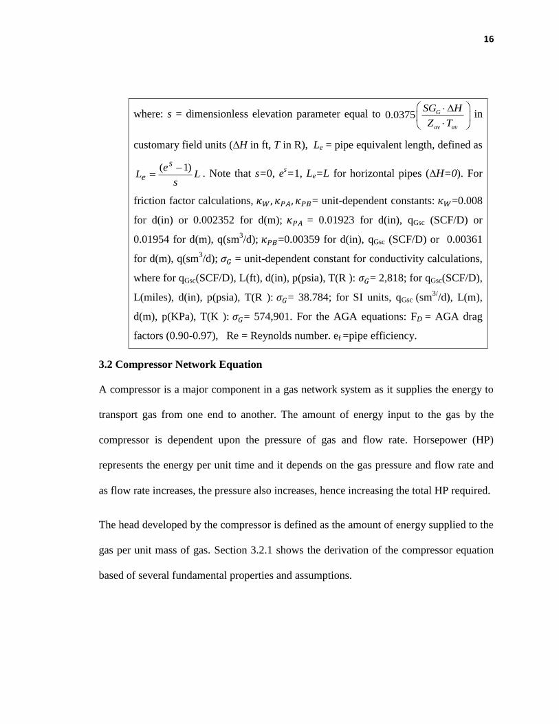
where: s = dimensionless elevation parameter equal to 0.0375 G

av av

SG H

Z T

in

customary field units (∆H in ft, T in R), Le = pipe equivalent length, defined as

Ls

eL

s

e)1(

. Note that s=0, es=1, Le=L for horizontal pipes (∆H=0). For

friction factor calculations, = unit-dependent constants: =0.008

for d(in) or 0.002352 for d(m); = 0.01923 for d(in), qGsc (SCF/D) or

0.01954 for d(m), q(sm3/d); =0.00359 for d(in), qGsc (SCF/D) or 0.00361

for d(m), q(sm3/d); = unit-dependent constant for conductivity calculations,

where for qGsc(SCF/D), L(ft), d(in), p(psia), T(R ): = 2,818; for qGsc(SCF/D),

L(miles), d(in), p(psia), T(R ): = 38.784; for SI units, qGsc (sm3/

/d), L(m),

d(m), p(KPa), T(K ): = 574,901. For the AGA equations: FD = AGA drag

factors (0.90-0.97), Re = Reynolds number. ef =pipe efficiency.

3.2 Compressor Network Equation

A compressor is a major component in a gas network system as it supplies the energy to

transport gas from one end to another. The amount of energy input to the gas by the

compressor is dependent upon the pressure of gas and flow rate. Horsepower (HP)

represents the energy per unit time and it depends on the gas pressure and flow rate and

as flow rate increases, the pressure also increases, hence increasing the total HP required.

The head developed by the compressor is defined as the amount of energy supplied to the

gas per unit mass of gas. Section 3.2.1 shows the derivation of the compressor equation

based of several fundamental properties and assumptions.

17

3.2.1 Derivation of Compressor Equation for Single-Phase Flow

There are different processes by how gas is compressed and they are categorized as

isothermal, adiabatic (isentropic) and polytropic compression. Isothermal compression is

a process where the gas pressure and volume are compressed as such that there will be no

changes in temperature. Hence, the least amount of work done is through isothermal

compression with comparison to other types of gas compression. However, this process is

only of theoretical interest since it is virtually impossible to maintain temperature

constant while compression is taking place (Menon, 2005).

On the other hand, adiabatic compression is essentially a process defined by zero heat

transfer occurring between any molecules in contact with the gas. Isotropic is referred as

when an adiabatic process is frictionless. Polytropic compression is intrinsically similar

to adiabatic compression, except that there is no need for zero heat transfer in the process.

The relationship between pressure and volume for both an adiabatic and a polytropic

process is as follows:

pnPV C (3.9)

and

1 1 2 2p pn n

PV PV (3.10)

where: P = pressure, V= volume, C= constant

np = polytropic exponent (polytropic process). Note that np= γ = ratio of specific

heats of gas if the process is adiabatic (isentropic).

18

Hence, work done by compression could then be calculated by integrating the expression

(3.10):

2

1

p

pW dp (3.11)

where: W = work done by compression. Taking the integral of expression (3.11) then

yields, for a polytropic process:

1

( ) 11

p

p

n

np j

i i

p i

n pW p v

n p

(3.12)

Since energy could be defined as work done by a force, the power required to run the

compressor station could then be expressed in the context of gas flow rate and discharge

pressure of compression station:

HP = M W (3.13)

Substituting M =ρsc qsc and expression (3.12) into expression (3.13), the equation written

in terms of Power is as below:

1

( ) 11

p

p

ij

n

np j

sc g i i

p i

n pHP q p v

n p

(3.14)

where: HP = Power,

M = Mass Flow Rate,

sc = Density at standard conditions

19

ijgq = Gas Flow Rate

Using real gas law, pV ZRT can be substituted in the expression (3.14) to account for

average compressibility factor effects.

Considering units conversion for oilfield units standard, a rather common form of the

formula for multistage compression, which assumes intercooling and equal compression

ratios across all stages, is:

1

10.0857 ( ) ( ) 1

1

p

p st

ij

n

n nst p j

G i av

p i

n n pHP q T Z

n p

(3.15)

where:

HP = compressor horsepower, HP

np = polytropic coefficient or ratio of specific heats (if adiabatic), dimensionless

nst = number of compression stages,

= suction temperature of gas, R

= gas flow rate, MMSCFD

= entry suction pressure of gas, psia

= final discharge pressure of gas, psia

= average gas compressibility, dimensionless

= compressor adiabatic (isentropic) or polytropic efficiency, decimal value (0.75-0.85)

20

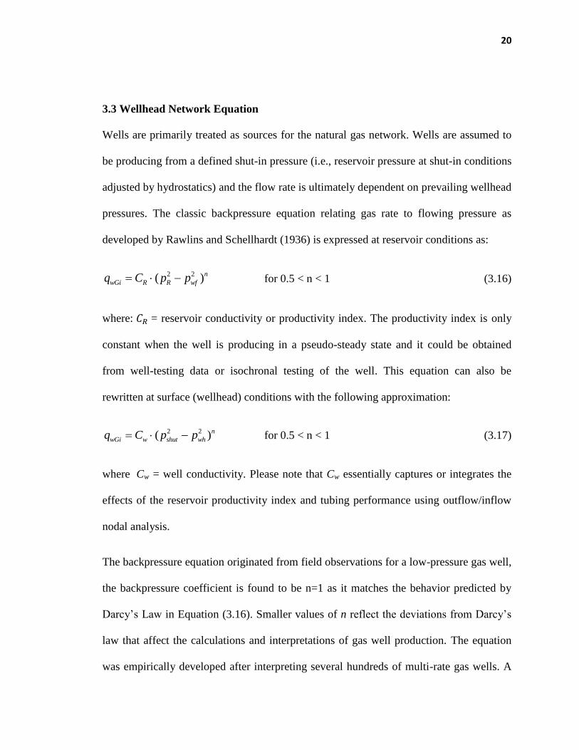
3.3 Wellhead Network Equation

Wells are primarily treated as sources for the natural gas network. Wells are assumed to

be producing from a defined shut-in pressure (i.e., reservoir pressure at shut-in conditions

adjusted by hydrostatics) and the flow rate is ultimately dependent on prevailing wellhead

pressures. The classic backpressure equation relating gas rate to flowing pressure as

developed by Rawlins and Schellhardt (1936) is expressed at reservoir conditions as:

2 2( )n

wGi R R wfq C p p

for 0.5 < n < 1 (3.16)

where: = reservoir conductivity or productivity index. The productivity index is only

constant when the well is producing in a pseudo-steady state and it could be obtained

from well-testing data or isochronal testing of the well. This equation can also be

rewritten at surface (wellhead) conditions with the following approximation:

2 2( )n

wGi w shut whq C p p for 0.5 < n < 1 (3.17)

where Cw = well conductivity. Please note that Cw essentially captures or integrates the

effects of the reservoir productivity index and tubing performance using outflow/inflow

nodal analysis.

The backpressure equation originated from field observations for a low-pressure gas well,

the backpressure coefficient is found to be n=1 as it matches the behavior predicted by

Darcy’s Law in Equation (3.16). Smaller values of n reflect the deviations from Darcy’s

law that affect the calculations and interpretations of gas well production. The equation

was empirically developed after interpreting several hundreds of multi-rate gas wells. A

21

linear trend was actually scrutinized on the log-log plot of rate versus delta pressure-

squared (Golan and Whitson, 1991). It was observed that the pressure squared actually

accounts for the fluid properties that are highly dependent on pressure such as the gas

viscosity and compressibility factor.

3.4 Newton-Based Gas Network Model

Gas network analysis entails the calculations of flow capacity of each pipeline segment

(B-segments) and pressure at each pipe junction (N-nodes) in a network. This can be

accomplished either by making pipe flows the primary unknowns of the problem (i.e., the

q-formulation, or nodal-loop formulation, consisting of “B” unknowns) or by making

nodal pressures the primary unknowns (i.e., the p-formulation, or nodal formulation with

“N-1” unknowns). In looped networks, a ∆q-formulation or loop formulation, where loop

flow corrections become the primary unknowns in the problem, is also possible. In all

cases, in order to achieve mathematical closure, the number of available equations must

match the number of unknowns in the formulation.

3.4.1 Nodal-loop or q-formulation

In a nodal-loop formulation, network governing equations are articulated via the

application of mass conservation principles applied to each node and energy conservation

principles applied to each loop in the system in order to solve for all “B” unknowns (i.e.,

individual pipe flow rates). The approach is known as the “nodal-loop” formulation

because of the source of the equations being used, but also as a “q-formulation” because

22

of the type of the unknowns being solved for. Mass conservation written at each node

requires that the algebraic sum of flows entering and leaving the node must be equal to

zero. In other words,

0 DSqq out

Gij

in

Gij written for each node and flows converging to it (3.18)

“N” equations of mass conservation of this type can be written at each nodal junction in

the system. Equation (3.18) is recognized as the 1st law of Kirchhoff of circuits, in direct

analogy to the analysis of flow of electricity in electrical networks. “S” and “D” represent

any external supply or demand (sink/source) specified at the node. For gas networks, this

equation is actually a mass conservation statement even though it is explicitly written in

terms of volumetric rates evaluated at standard conditions. Equation (3.18) provides “N-

1” admissible equations because only “N-1” nodal equations are linearly independent. In

this nodal-loop formulation, “LP” additional equations are also needed to exactly balance

the number of unknowns “B” [ since (N-1) + LP = B ] and achieve mathematical closure

in the formulation. These equations are formulated by applying the 2nd

law of Kirchhoff

to every independent loop. In any closed loop, the algebraic sum of all pressure drops

must equal zero. This is true of any closed path in a network, since the value of pressure

at any point of the network must be the same regardless of the closed path followed to

reach the point. The signs of the pressure drops are taken with respect to a consistent

sense of rotation around the loop, and the loop equation is written as:

2 2( ) 0loop

i j

ij

p p

written for each pipe within any given loop (3.19)

23

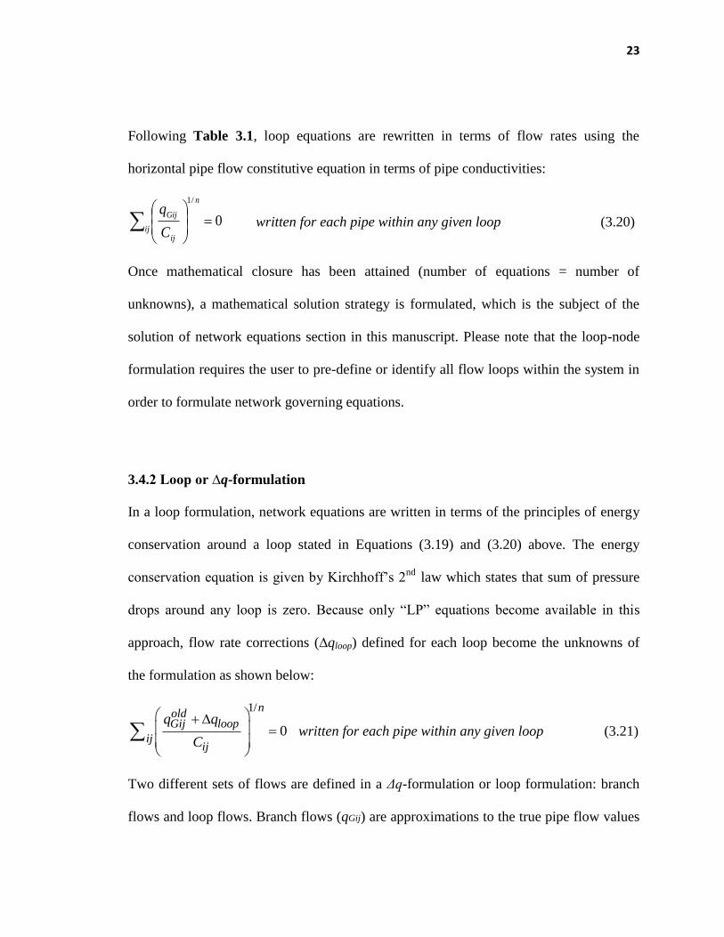
Following Table 3.1, loop equations are rewritten in terms of flow rates using the

horizontal pipe flow constitutive equation in terms of pipe conductivities:

0

/1

ij

n

ij

Gij

C

q written for each pipe within any given loop (3.20)

Once mathematical closure has been attained (number of equations = number of

unknowns), a mathematical solution strategy is formulated, which is the subject of the

solution of network equations section in this manuscript. Please note that the loop-node

formulation requires the user to pre-define or identify all flow loops within the system in

order to formulate network governing equations.

3.4.2 Loop or ∆q-formulation

In a loop formulation, network equations are written in terms of the principles of energy

conservation around a loop stated in Equations (3.19) and (3.20) above. The energy

conservation equation is given by Kirchhoff’s 2nd

law which states that sum of pressure

drops around any loop is zero. Because only “LP” equations become available in this

approach, flow rate corrections (∆qloop) defined for each loop become the unknowns of

the formulation as shown below:

1/

0

noldGij loop

ijij

q q

C

written for each pipe within any given loop (3.21)

Two different sets of flows are defined in a Δq-formulation or loop formulation: branch

flows and loop flows. Branch flows (qGij) are approximations to the true pipe flow values

24

and loop flows (Δqloop) are introduced to correct prevailing branch flows in order to yield

the actual values. Initial values for both branch flow and loop flows are required for the

iterative procedure. When Equation (3.21) is satisfied for all loops, convergence has been

attained. This formulation also requires the user to identify all flow loops within the

network system prior to formulating associated governing equations. Since a number of

permutations of independent loops are possible for any given large network, this

formulation further requires optimization strategies for the optimal set of loops that

would be used during the solution strategy.

3.4.3 Nodal or p-formulation

In a nodal formulation, network equations are written on the basis of the principle of

nodal mass conservation (continuity) alone. This yields “N-1” linearly independent

equations that can be used to solve for “N-1” unknowns (i.e., nodal pressures) since one

nodal pressure is assumed to be specified within the system. In this formulation, nodal

mass conservation statements in Equation (3.18) are rewritten in terms of nodal pressures

using the pipe flow constitutive equations in Table 3.1, which yields for horizontal flow:

0)( 22 ij

n

jiij DSppC (3.22)

In Equation (3.22), fluid flowing into the node is assumed positive and fluid leaving the

node is given a negative sign. External supplies and demands (sink/sources) specified at

the node are also considered. The p-formulation or nodal method does not require the

identification or optimization of loops and the application of the 2nd

law of Kirchhoff is

circumvented. However in a p-formulation, the resulting set of governing equations is

25

more complex and more non-linear than the ones found in the loop- and nodal-loop

counterparts since pressures are expressed in squared difference. In addition, the method

is well-known to suffer from poor convergence characteristics or severe sensitivity to

initialization conditions when Newton-Raphson protocols are implemented to achieve a

solution (Ayala, 2012; Larock et al., 2000, Osiadacz, 1987).

With that, this study shows that the highly non-linear nodal equations in Equation (3.22)

can be readily transformed into linear equations to circumvent this problem. As a result,

the poor convergence characteristics of the p-formulation are eliminated, convergence is

made independent of user-defined initial guesses for nodal pressures and flow rates, and

the needs of calculating expensive Jacobian formulations and associated derivatives are

also removed. Concurrently, the analog method which will be discussed below retains the

advantages of the p-formulation in terms of not requiring loop identification protocols.

26

CHAPTER 4

THE LINEAR PRESSURE ANALOG MODEL

4.1 Linear Analog Model

Regardless of the type formulation used, all Newton-based methods are prone to lack of

convergence and sensitivity to initial guesses, with the nodal formulation being the most

susceptible of all. Presumption of appropriate initial guesses is the key for solving gas

network equations for every existing method. In order to circumvent network solution

convergence problems of currently available methods and their potentially costly

implementation, this study proposes the implementation of a linear-pressure analog

model for the solution of the highly non-linear equations in natural gas transportation

networks. The method consists of defining an alternate, analog system of pipes that obey

a much simpler pipe constitutive equation, i.e., a linear-pressure analog flow equation,

which is written for horizontal pipes as follows:

)( jiijGij ppLq (4.1)

where Lij is the value of the linear pressure analog conductivity. Note that Equation (4.1)

uses the flow-pressure drop dependency prescribed by the Hagen-Poiseuille’s law for

liquid flow in laminar conditions. Consequently, the proposed analog seeks to map the

highly non-linear gas flow network problem into the much more tractable liquid network

problem for laminar flow conditions. When gas pipe flows are written in terms of such a

linear pressure analog, nodal mass balances used in p-formulations (Equation 3.22)

27

collapse to a much simpler (and more importantly, linear) set of algebraic equations

shown in Equation (4.2):

( ) 0ij i jL p p S D (4.2)

which can be simultaneously solved for all nodal pressures in the network using any

standard method of solution of linear algebraic equations—as opposed to its non-linear

counterpart of Equation (3.22).

Linear-pressure analog conductivities are straightforwardly calculated as a function of

actual pipe conductivities according to the following transformation rule:

ijijij CTL (4.3)

where Lij is the conductivity of the linear-pressure analog pipe which conforms to the

linear equation in (4.1), and Cij is the actual pipe conductivity conforming to the

generalized flow equation definition in Table 3.1 that for horizontal pipes becomes:

n

jiijGij ppCq )( 22 (4.4)

In Equation (4.4), n is equal to 0.50 as prescribed by the generalized gas flow equation.

It is straightforwardly demonstrated that the variable Tij in Equation (4.3), i.e., the analog-

pipe conductivity transform, is given by the expression:

1

21

ij

ijr

T

(4.5)

This analog-pipe transform is a dimensionless quantity that enforces the flow-rate

equivalency of Equations (4.1) and (4.4) for the pipe of interest. The dimensionless

28

analog-pipe transform turns out to be solely dependent on rij, i.e., the pressure ratio

between the pipe end pressures as shown in Equation (4.6):

j

iij

p

pr (4.6)

where i=upstream node and j=downstream node as defined in Equations (4.1) and (4.4).

The derivation of linear-pressure analog conductivity is shown in Figure 4.1 below.

( ) (

)

( ) (

)

( )( )

( )(

)

(

)

(

)

√

√

Figure 4.1: Derivation of Linear-Pressure Analog Conductivity

29

Because pressure ratios are always higher than one (pi > pj for fluid to flow, given that

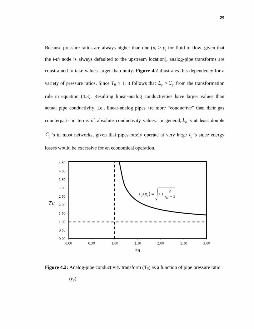
the i-th node is always defaulted to the upstream location), analog-pipe transforms are

constrained to take values larger than unity. Figure 4.2 illustrates this dependency for a

variety of pressure ratios. Since Tij > 1, it follows that ijij CL from the transformation

rule in equation (4.3). Resulting linear-analog conductivities have larger values than

actual pipe conductivity, i.e., linear-analog pipes are more “conductive” than their gas

counterparts in terms of absolute conductivity values. In general, ijL ’s at least double

ijC ’s in most networks, given that pipes rarely operate at very large ijr ’s since energy

losses would be excessive for an economical operation.

Figure 4.2: Analog-pipe conductivity transform (Tij) as a function of pipe pressure ratio

(rij)

30

Once the linear-analog transform has been applied, all unknown nodal pressures in the

network can be calculated by solving the resulting linear set of algebraic equations. Since

actual pressure ratios (rij) are not known in advance, the linear analog method starts its

first iteration with the condition ijij CL . Note that no initial guesses for nodal pressure

values or pipe flow rates are needed. However, once a first set of estimated nodal

pressures become available during the first iteration, interim pressure ratios ( 'ijr ), pipe

conductivities, and pipe flow rates can be calculated. In this first iteration, resulting

pressure drops would become significantly overestimated because pipe analogs are forced

to be less conductive than they should since ijij CL instead of ijij CL . Interim

pressure ratios ( 'ijr ) thus start at significantly overstated values during the first iteration

and, upon successive substitutions and after a few inexpensive iterations, they steadily

adjust to actual rij. When this occurs, the non-linear network problem has been fully

solved. Convergence is attained when any further nodal pressure update would become

inconsequential within a prescribed tolerance (e.g. ).

Because pressure drops are always overestimated in the first analog iterations, upstream

pressures will be underestimated if downstream pressures are specified. This may force

upstream pressure to take negative values early during the iterative procedure. For these

cases, a direct application of Equation (4.6) would violate the analog principle that

requires all pipe pressure ratios to be positive and higher than 1. Therefore, if negative

downstream pressure is calculated, Value of pressure ratio calculations is defaulted to a

31

minimum value (equal to atmospheric pressure) and upstream pressure is displaced

accordingly using the calculated pipe pressure drop. In other words,

| ( ) | 14.7

14.7

i j

ij

p pr

(4.7)

Please note that this type of adjustment can be avoided altogether if instead of initializing

the analog method with the condition ijij CL (first iteration), one uses a multiple of the

pipe conductivity (such as 2ij ijL C or 3ij ijL C ) for initialization. Such initialization

makes the linear analog more conductive from the onset, thus avoiding unnecessarily

large pressure loss estimations during the first iteration.

It can be shown that the proposed analog method has a remarkably stable performance.

This is due in part because its iterations do not necessitate user-prescribed guesses and

each individual iteration solves a feasible liquid-flow scenario with a unique solution.

This is to be compared to the potentially unconstrained behavior of Newton-Raphson

protocols, which demand the use of good initializations (i.e., initial “guesses” sufficiently

close to the actual solution) for convergence to be possible. The proposed approach is

also fundamentally different from the Linear Theory method (Wood and Carl, 1972) in

the sense that it always relies on exact solutions to well-behaved linear-analog liquid

fluid flow problems for each of its iterations. The Linear Theory Method, instead, relies

on solving approximate sets of linearized equations, which do not necessarily correspond

32

to physically-constrained systems and thus is susceptible to spurious numerical

oscillations.

Note that the value of ijC in the transformation in Equation (4.3) remains constant

during the iteration process for all flow equations where friction factor (and thus pipe

conductivity as per its definition in Table 3.1) are defined to be independent of flow rate.

This is the case, for example, of the Weymouth and the AGA fully-turbulent friction

factor equations in Table 3.1. For all other flow-rate-dependent friction factor equations,

in order to preserve initial-guess-free nature of the solution process, the ijC estimation is

defaulted to that of flow-rate independent flow equation such as Weymouth. For all

subsequent iterations, ijC becomes simultaneously updated based on the most current

flow rate information using the friction factor expression of choice from Table 3.1. The

proposed workflow for the implementation of the linear-analog methodology is displayed

in Figure 4.3.

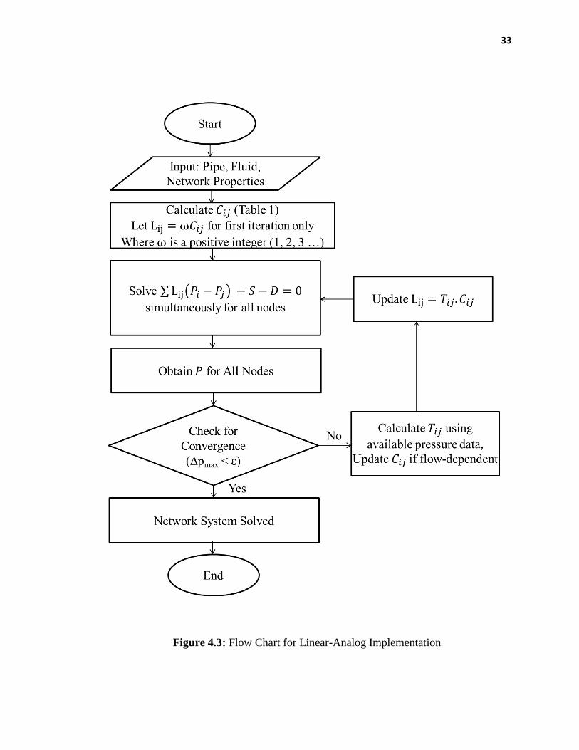
33

Figure 4.3: Flow Chart for Linear-Analog Implementation

34

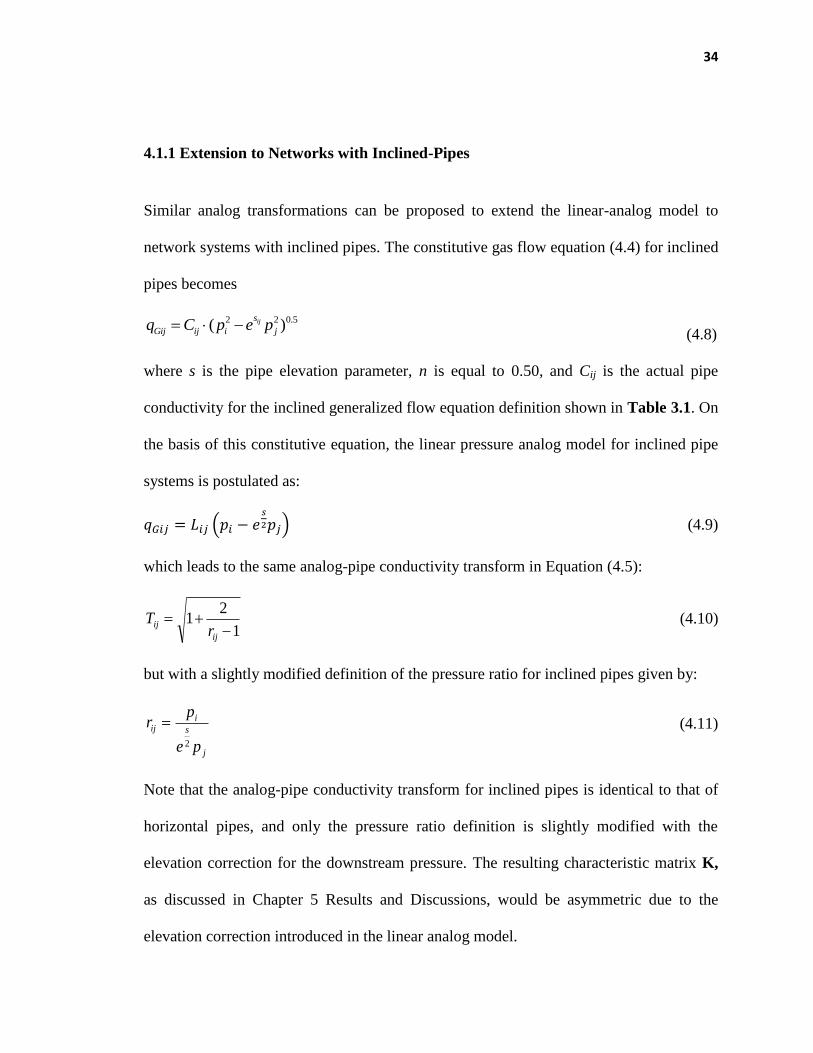
4.1.1 Extension to Networks with Inclined-Pipes

Similar analog transformations can be proposed to extend the linear-analog model to

network systems with inclined pipes. The constitutive gas flow equation (4.4) for inclined

pipes becomes

2 2 0.5( )ijs

Gij ij i jq C p e p (4.8)

where s is the pipe elevation parameter, n is equal to 0.50, and Cij is the actual pipe

conductivity for the inclined generalized flow equation definition shown in Table 3.1. On

the basis of this constitutive equation, the linear pressure analog model for inclined pipe

systems is postulated as:

(

) (4.9)

which leads to the same analog-pipe conductivity transform in Equation (4.5):

1

21

ij

ijr

T

(4.10)

but with a slightly modified definition of the pressure ratio for inclined pipes given by:

j

s

iij

pe

pr

2

(4.11)

Note that the analog-pipe conductivity transform for inclined pipes is identical to that of

horizontal pipes, and only the pressure ratio definition is slightly modified with the

elevation correction for the downstream pressure. The resulting characteristic matrix K,

as discussed in Chapter 5 Results and Discussions, would be asymmetric due to the

elevation correction introduced in the linear analog model.

35

However, it is also possible to redefine the linear-analog transform for inclined pipes in

order to preserve the symmetry of the characteristic matrix K, whenever desired, if the

application of efficient Cholesky algorithms is deemed of importance. Characteristic

matrix symmetry can be preserved by implementing the analog constitutive equation in

Equation (4.1) for inclined pipes, reproduced below:

)( jiijGij ppLq (4.12)

which would lead to a different analog-pipe conductivity transform than the one used

thus far:

√

( ) (4.13)

and which uses the same conventional pressure ratio definition:

(4.14)

This alternative approach would lead to linear algebraic equations with a symmetric

characteristic matrix. All proposed analog methods are summarized in the Table 4.1

below.

Table 4.1: Summary of Linear-Pressure Analog Constitutive Equations ( )

Network Type Linear-Pressure Analog

Constitutive Equation

Analog Conductivity Transform, Tij

Horizontal Pipes

(for a symmetric

characteristic matrix)

( ) √

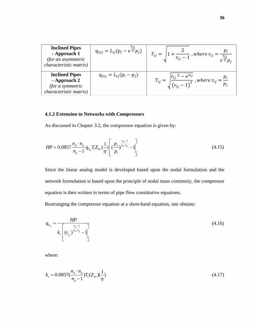
36

4.1.2 Extension to Networks with Compressors

As discussed in Chapter 3.2, the compressor equation is given by:

1

10.0857 ( ) ( ) 1

1

p

st p

ij

n

n nst p j

G i av

p i

n n pHP q T Z

n p

(4.15)

Since the linear analog model is developed based upon the nodal formulation and the

network formulation is based upon the principle of nodal mass continuity, the compressor

equation is then written in terms of pipe flow constitutive equations.

Rearranging the compressor equation at a short-hand equation, one obtains:

1

( ) 1

ij p

st p

ij

G n

n n

c c

HPq

k r

(4.16)

where:

10.0857( ) ( )( )

1

st p

c i av

p

n nk T Z

n

(4.17)

Inclined Pipes

- Approach 1

(for an asymmetric

characteristic matrix)

√

Inclined Pipes

- Approach 2

(for a symmetric

characteristic matrix)

√

( )

37

The total compressor ratio for a compression station is calculated as the ratio of its final

compressor discharge pressure to its entry suction pressure:

ij

j

c

i

pr

p (4.18)

In order to construct linear sets of equations from coupling compressors, the compression

ratio is assumed to be the target variable that needs to be specified by the user. For such

scenarios,

.  ij c jG iCq HP (4.19)

where the compressor constant is given as:

1

1

1p

st pn n

cij n

c cij

C

k r

[MMSCD/HP] (4.20)

The compressor equation is then incorporated into the gas network system by predefining

the compressor desired total compression ratio, which results in the determination of the

horsepower required for the compressor to be solved for as an unknown within the

system of equations.

4.1.3 Extension to Networks with Wellheads

The wellhead equation at surface (wellhead) conditions can be written as:

2 2.( )  i

n

wG w shut whpCq p for 0.5 < n < 1 (4.21)

38

This constitutive relationship retains a form identical to that of the pipeline gas flow

equation and hence a similar analog transformation could be applied to linearize the

wellhead equation. The backpressure equation is similar to the way the generalized pipe

equation is expressed, while the coefficients n and vary for different reservoir and

tubing properties for the backpressure equation.

The linear analog equation for any wellhead in the network system is then given by:

( )wGi w shut whq L p p (4.22)

Linear-pressure analog conductivities for a wellhead are again computed as a function of

actual well conductivities according to the following transformation rule:

w w wL T C (4.23)

where Lw is the wellhead conductivity in the linear-pressure analog model which

conforms to the linear equation in (4.22), and Cw is the actual well conductivity

conforming to the wellhead equation (4.21). The analog-well conductivity transform Tw

in Equation (4.23) now becomes a function of the well flow exponent (which ranges from

0.5 to 1) and the well shut-in pressure, as shown below:

1 2 11 1(1 ) (1 )n n n

w shut

w w

T pr r

(4.24)

where the wellhead pressure ratio, wr is given by the ratio of shut-in pressure, shutp to

wellhead pressure, whp .

shutw

wh

pr

p (4.25)

39

Since rw is not available until the next iteration, wL is to be approximated by the

following expression during the first iteration:

2 1n

w shut wL p C (4.26)

Please note that 2 1n

shutp

is the constant that appears in the wTterm and hence it should be

introduced in the first iteration to ensure a reasonable conductivity approximation in the

first iteration.

Figure 4.4 depicts the dependency of the analog-well conductivity transform for a range

of flow exponents. Since Tw > 1, it follows that ijij CL from the transformation rule in

equation (4.23). Similarly, resulting linear-analog conductivities have larger values than

actual well conductivity, i.e., linear-analog wells are more “conductive” or “productive”

than their gas counterparts in terms of the absolute values of their conductivity. In Figure

4.4, Pshut was assumed to be 100 psia for illustration purposes.

40

Figure 4.4 Analog-well conductivity transform (Tw) as a function of well pressure

ratio (rw) (for Pshut = 100 psia)

Similar to the discussion for pipes, there may be occasions where wellhead pressures can

be estimated to be negative during the first iterations. This is due to the fact that early

analogs tend to overestimate actual pressure drops in the system. For these cases, since

pressure ratios must always be positive and higher than one, the following expression is

used when wellhead pressure is deemed to be negative by early iterations:

14.7

shutw

pr

(4.27)

1

10

100

1000

1 1.5 2 2.5 3 3.5

Tw

rw

n=1

n=0.9

n=0.8

n=0.7

n=0.6

n=0.5

41

CHAPTER 5

RESULTS AND DISCUSSIONS

5.1 Case Study 1: Horizontal Pipe Network System

For this case study, the horizontal network system depicted on Figure 1.1 is analyzed

using the generalized gas flow equation coupled with AGA-fully turbulent friction factor

calculations. An average flowing temperature of 75 ºF and an average compressibility

factor of 0.90 are assumed for the entire system for illustration purposes; however, the

methodology would remain unchanged if each pipe were to be considered to operate at

different average temperatures and if compressibility factors were calculated in terms of

standard natural gas correlations. Those variables would only affect the update of actual

pipe conductivities Cij described in the solution protocol of Figure 4.3. The network

handles a gas with a specific gravity of 0.69 and all pipes are assumed to be carbon steel

(e = 0.0018 in), horizontal, 30-miles long and NPS 4 Sch 40, except for pipes (1,2), (2,3),

(1,4) and (4,7) which are NPS 6 Sch 40. The pressure specification is given at node 9 and

it is set at 130 psia. Based on the implementation of the solution protocol in Figure 4.3,

the gas network under study generates the following linear system of algebraic equations

in terms of nodal pressures:

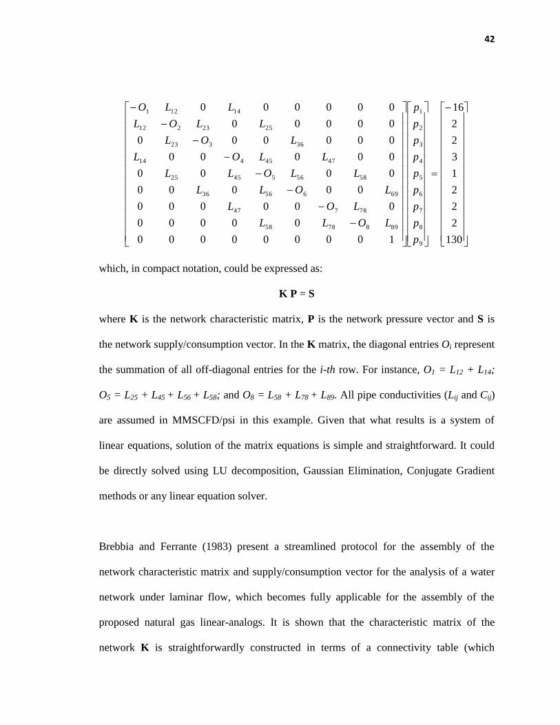
42

130

2

2

2

1

3

2

2

16

100000000

00000

000000

00000

0000

00000

000000

00000

000000

9

8

7

6

5

4

3

2

1

8987858

78747

6965636

585654525

4745414

36323

2523212

14121

p

p

p

p

p

p

p

p

p

LOLL

LOL

LOLL

LLOLL

LLOL

LOL

LLOL

LLO

which, in compact notation, could be expressed as:

K P = S

where K is the network characteristic matrix, P is the network pressure vector and S is

the network supply/consumption vector. In the K matrix, the diagonal entries Oi represent

the summation of all off-diagonal entries for the i-th row. For instance, O1 = L12 + L14;

O5 = L25 + L45 + L56 + L58; and O8 = L58 + L78 + L89. All pipe conductivities (Lij and Cij)

are assumed in MMSCFD/psi in this example. Given that what results is a system of

linear equations, solution of the matrix equations is simple and straightforward. It could

be directly solved using LU decomposition, Gaussian Elimination, Conjugate Gradient

methods or any linear equation solver.

Brebbia and Ferrante (1983) present a streamlined protocol for the assembly of the

network characteristic matrix and supply/consumption vector for the analysis of a water

network under laminar flow, which becomes fully applicable for the assembly of the

proposed natural gas linear-analogs. It is shown that the characteristic matrix of the

network K is straightforwardly constructed in terms of a connectivity table (which

43

matches each pipe branch with its upstream and downstream nodes) available from input

data. This assembly protocol streamlines the identification of the location of each pipe

conductivity contribution within the characteristic matrix as a function of the information

in the connectivity table. The assembly protocol also honors the presence of boundary

conditions, such as pressure and supply/demand specifications. It is recognized that the

matrix K is a banded matrix, which is a property that can be used to save storage space

during computations. The half-bandwidth of this matrix is a function of the maximum

difference in the numbers of any two nodes connected to each other; in particular, the half

bandwidth is equal to that maximum difference plus one because of the presence of the

diagonal. From Figure 1.1, this maximum difference is equal to 3, corresponding to the

difference between the node numbers of pipes (5,8) or (1,4) for instance. This yields a

half-bandwidth of 4 which is evident in the matrix above. A properly numbered large

network system can be made to have small half-bandwidths, thus making large storage

savings possible.

By moving all known pressure-node matrix entries (L69 and L89) to the consumption

vector, the characteristic matrix can also become fully symmetric, i.e., K = KT. This

property can not only be used to save additional storage space (i.e., only the upper or

lower portion of the matrix needs to be stored) but also to implement efficient linear

equation solvers that fully exploit this property. A system of linear equations with a

positive-definite and symmetric matrix can be efficiently and inexpensively solved using

Cholesky decomposition, which can be shown to be roughly twice as efficient as LU

44

decomposition for solving systems of linear equations (Press et al., 2007). Matrix K is

positive-definite because it is symmetric and diagonally-dominant with positive diagonal

entries. Note that positive diagonal entries are obtained by multiplying all matrix and

right-hand-side vector entries by -1 for all equations other than the dummy constant-

pressure specification.

The inexpensive, steady convergence nature of the proposed protocol is depicted in

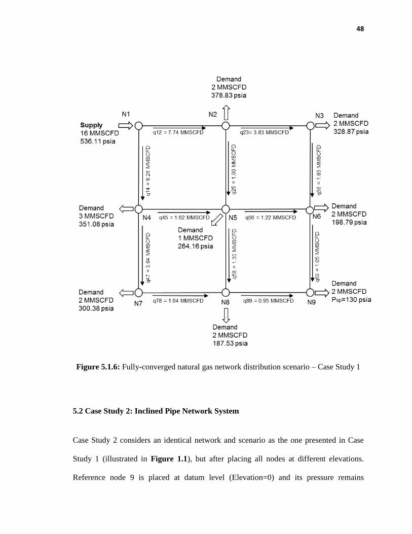
Figures 5.1.1 to 5.1.5 for the iterative solution of the case under study. The final

converged solution is provided in Figure 5.1.6, which fully satisfies the original set of

highly non-linear gas network equations. Note, again, that no user-provided guesses of

pressure or flow rate are needed at any point of the protocol and that just a few

inexpensive iterations are needed for the protocol to reach the immediate neighborhood

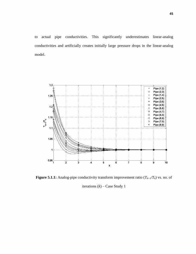
of the actual solution. Figure 5.1.1 demonstrates that the values of analog-pipe

conductivity transform ratios steadily converge to their true values as the number of

iterations increases. This can be further visualized in Figure 5.1.2, where it becomes

evident that pipe pressure ratios progressively stabilize as the number of iteration

increases. The relationship between the analog-pipe conductivity transforms and pressure

ratios (originally illustrated in Figure 4.3) is continuously honored during the process as

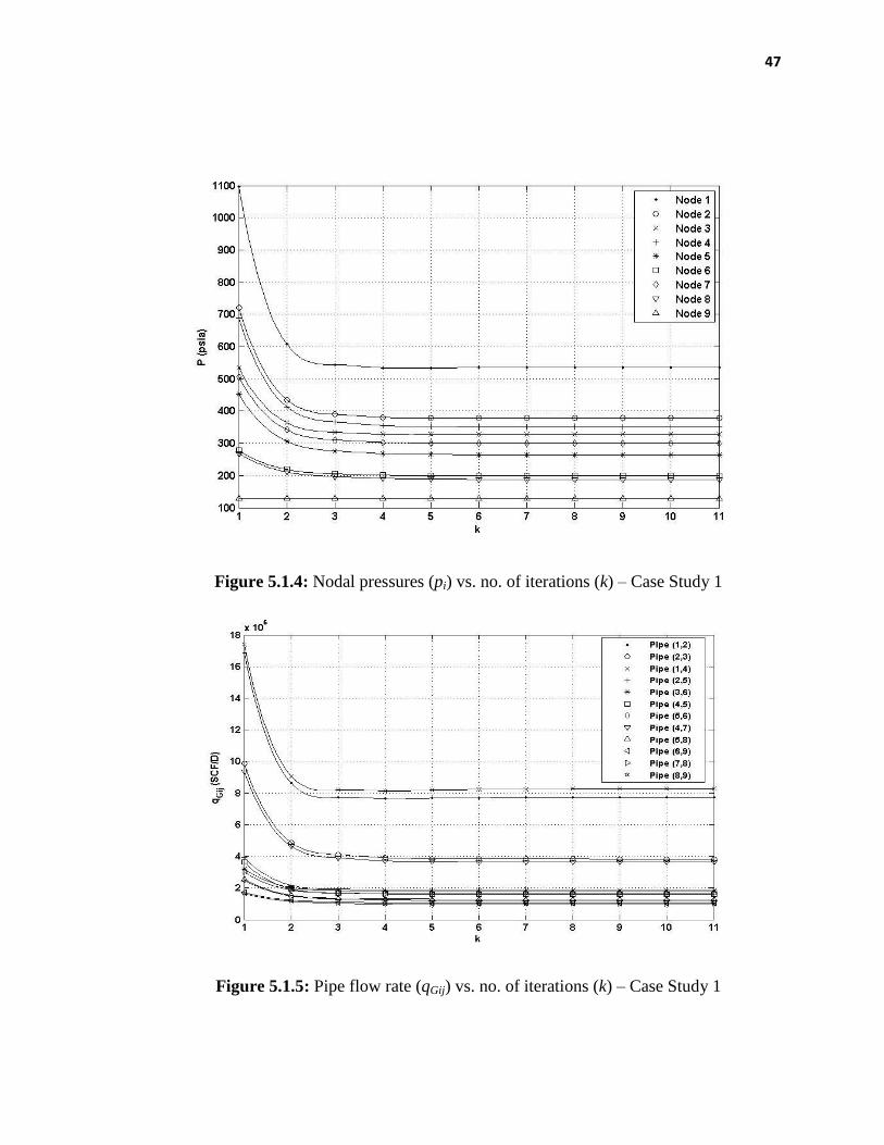
demonstrated by Figure 5.1.3. As a result, nodal pressures and flow rates steadily

approach their true values as the protocol progresses, as shown in Figure 5.1.4 and

Figure 5.1.5, respectively. These figures demonstrate that nodal pressures and flow rates

are initially overestimated because linear analog conductivities were initially made equal

45

to actual pipe conductivities. This significantly underestimates linear-analog

conductivities and artificially creates initially large pressure drops in the linear-analog

model.

Figure 5.1.1: Analog-pipe conductivity transform improvement ratio (Tk+1/Tk) vs. no. of

iterations (k) – Case Study 1

46

Figure 5.1.2: Pressure ratio (rij) vs. no. of iterations (k) – Case Study 1

Figure 5.1.3: Analog-pipe conductivity transform (Tij) vs. pressure ratio (rij) – Case

Study 1

47

Figure 5.1.4: Nodal pressures (pi) vs. no. of iterations (k) – Case Study 1

Figure 5.1.5: Pipe flow rate (qGij) vs. no. of iterations (k) – Case Study 1

48

Figure 5.1.6: Fully-converged natural gas network distribution scenario – Case Study 1

5.2 Case Study 2: Inclined Pipe Network System

Case Study 2 considers an identical network and scenario as the one presented in Case

Study 1 (illustrated in Figure 1.1), but after placing all nodes at different elevations.

Reference node 9 is placed at datum level (Elevation=0) and its pressure remains

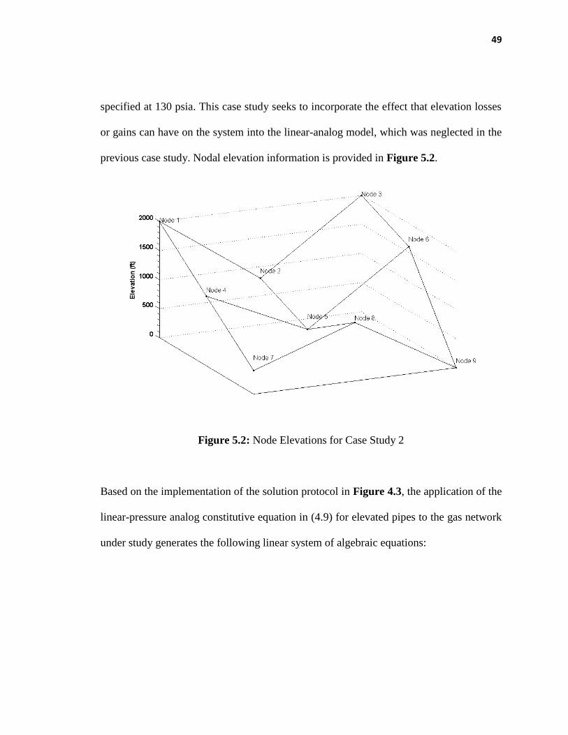
49

specified at 130 psia. This case study seeks to incorporate the effect that elevation losses

or gains can have on the system into the linear-analog model, which was neglected in the

previous case study. Nodal elevation information is provided in Figure 5.2.

Figure 5.2: Node Elevations for Case Study 2

Based on the implementation of the solution protocol in Figure 4.3, the application of the

linear-pressure analog constitutive equation in (4.9) for elevated pipes to the gas network

under study generates the following linear system of algebraic equations:

50

130

2

2

2

1

3

2

2

16

100000000

00000

000000

00000

0000

00000

000000

00000

000000

9

8

7

6

5

4

3

2

1

89

2/

87858

78

2/

747

69

2/

65636

58

2/

56

2/

54525

47

2/

45

2/

414

36

2/

323

25

2/

23

2/

212

14

2/

12

2/

1

89

78

69

5856

4745

36

2523

1412

p

p

p

p

p

p

p

p

p

LeOLL

LeOL

LeOLL

LeLeOLL

LeLeOL

LeOL

LeLeOL

LeLeO

s

s

s

ss

ss

s

ss

ss

which, in compact notation, is expressed as:

K P = S

In the new K characteristic matrix, the upper right portion of the matrix contains all the

“esij/2

” elevation corrections applicable to downstram nodes and the lower left portion of

the matrix contains conductivity information for the upstream nodes. Diagonal entries Oi

are no longer just the summation of all off-diagonal entries, given that elevation terms

must be taken into account for all cases where node “i” is found in the downstream

position. For instance, O1 = L12 + L14; but O5 = L25 es25/2

+ L45 es45/2

+ L56 + L58; and O8

= L58 es58/2

+ L78 es78/2

+ L89. All pipes conductivities (Lij and Cij) remain in MMSCFD/psi

in this example. The resulting characteristic matrix K remains banded but no longer

symmetric; therefore, the implementation of a Cholesky decomposition is no longer

possible. The resulting system of linear equations is then directly solved using any other

standard linear equation solver such as LU decomposition, Gaussian Elimination, or

Conjugate Gradient methods. Figure 5.2.1 to 5.2.5 present the results of such iterative

solution protocol which follows the workflow of Figure 4.3. Final converged values or

the actual network solution are displayed in Figure 5.2.6. As previously shown, analog

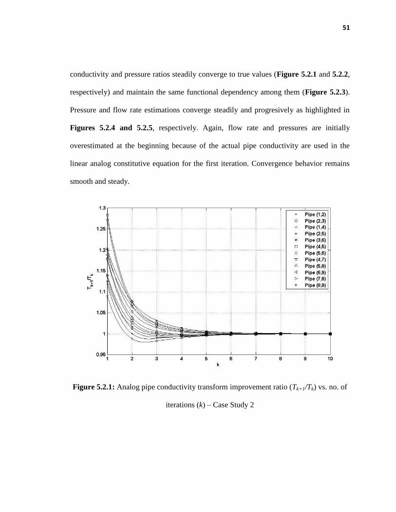
51

conductivity and pressure ratios steadily converge to true values (Figure 5.2.1 and 5.2.2,

respectively) and maintain the same functional dependency among them (Figure 5.2.3).

Pressure and flow rate estimations converge steadily and progresively as highlighted in

Figures 5.2.4 and 5.2.5, respectively. Again, flow rate and pressures are initially

overestimated at the beginning because of the actual pipe conductivity are used in the

linear analog constitutive equation for the first iteration. Convergence behavior remains

smooth and steady.

Figure 5.2.1: Analog pipe conductivity transform improvement ratio (Tk+1/Tk) vs. no. of

iterations (k) – Case Study 2

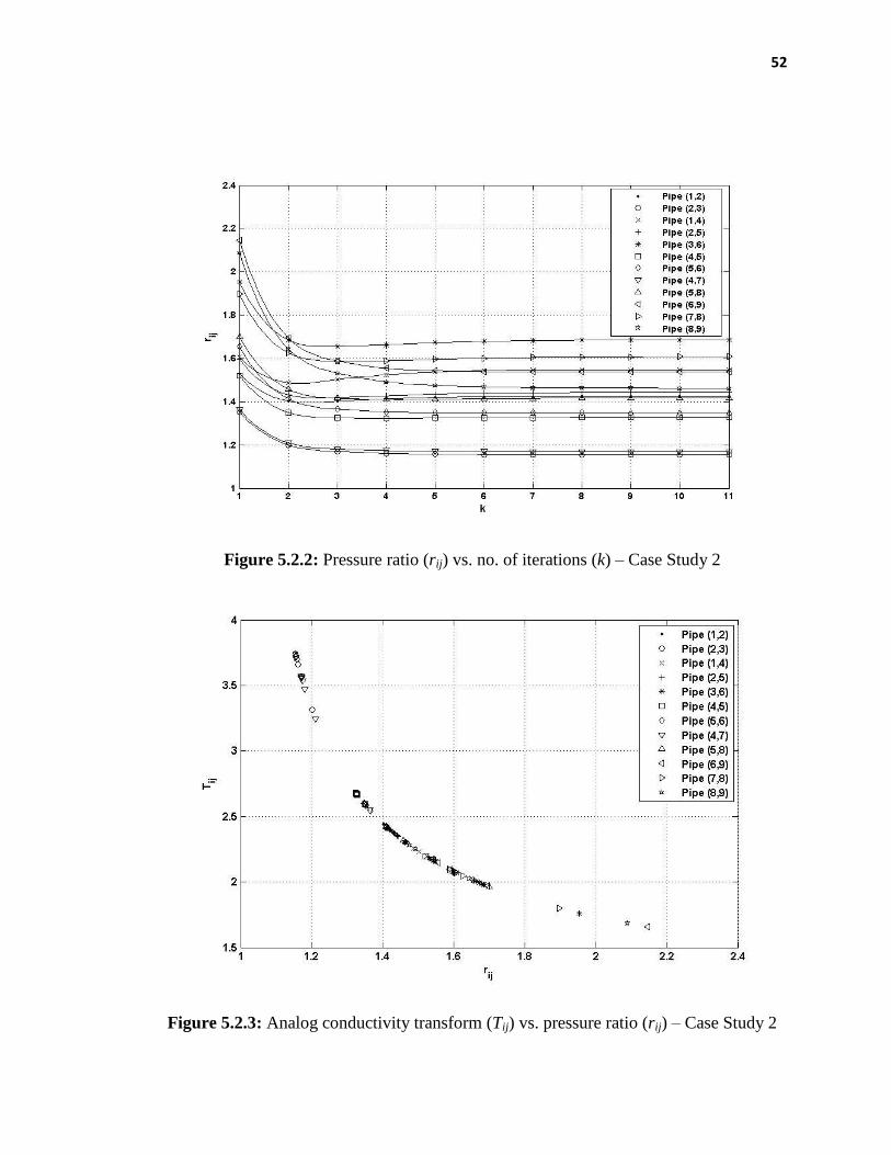
52

Figure 5.2.2: Pressure ratio (rij) vs. no. of iterations (k) – Case Study 2

Figure 5.2.3: Analog conductivity transform (Tij) vs. pressure ratio (rij) – Case Study 2

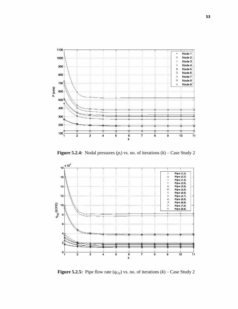
53

Figure 5.2.4: Nodal pressures (pi) vs. no. of iterations (k) – Case Study 2

Figure 5.2.5: Pipe flow rate (qGij) vs. no. of iterations (k) – Case Study 2

54

Figure 5.2.6: Fully-converged natural gas network distribution – Case Study 2

55

5.3 Case Study 3: Network System with Compression

Figure 5.3: Network Topology of Case Study 3

Case Study 3 models an identical network with the elevated-mode scenario as the one

presented in Case Study 2, but with an additional network component – a compressor. A

compressor is located in between node 5 and node 6 and pipe (4,5) and pipe (6,7) are

both 15 miles in length. The compressor is located at an elevation of 400 ft with respect

to the datum at node 11. Suction temperature and average gas compressibility of gas at

compressor are assumed to be 75 ºF and 0.9, respectively, with a polytropic exponent of

1.4 and a compressor efficiency of 0.9. The compressor is operating at a target

56

compression ratio of 2.50 with a single stage (nst=1). Node 11 is again specified at a

pressure of 130 psia. This case study attempts to incorporate a compressor system into

the linear-analog model, which was neglected in both the previous case studies. Similarly,

based upon the implementation of the solution protocol in Figure 4.3, the application of

the linear-pressure analog constitutive equations for elevated pipes in (4.9) coupled with

a compressor equation in (4.19) to the gas network under study generates the following

linear system of algebraic equations:

12 14

23 27

38

45 49

67

78 710

/2 /2

1 12 14

/2 /2

12 2 23 27

/2

23 3 38

/2 /2

14 4 45 49

45 5 56

/2

56 67 6 67

/2 /2

27 56 67 7 78 710

0 0 0 0 0 0 0 0

0 0 0 0 0 0 0

0 0 0 0 0 0 0 0

0 0 0 0 0 0 0

0 0 0 0 0 0 0 0

0 0 0 0 0 0 0 0

0 0 0 0 0 0

0 0

s s

s s

s

s s

C

s

s s

O e L e L

L O e L e L

L O e L

L O e L e L

L O C

r L O e L

L r L O e L e L

811

910

1011

1

2

3

4

5

7

/2838 78 8 811

/2949 9 910

/210710 910 10 1011

11

16

2

2

3

0

0

1

20 0 0 0 0

20 0 0 0 0 0 0 0

20 0 0 0 0 0 0

130 0 0 0 0 0 0 0 0 0 1

s

s

s

p

p

p

p

p

HP

p

pL L O e L

pL O e L

pL L O e L

p

0

which, in compact notation, is expressed as:

K P = S

In this particular case, the system of equations is constructed based upon the topology of

the compressor. Note that the P network pressure vector is slightly different from the two

previous case studies as the horsepower (HP) is represented here in node 6. The pressure

of the downstream node of the compressor is substituted as the unknown since the

pressure at node 6 is a function of the compression ratio given by 656

5

c

Pr

P . Hence the

pressure at node 6 is expressed as the pressure of node 5 by equating 6 56 5.cP r P . The

57

network consumption/supply vector S is similar except that there are no consumption and

supply at node 5 and 6. Characteristic matrix diagonal entries Oi are no longer just the

summation of all off-diagonal entries where compressors are defined, for example, as it is

at node 5 and node 6 in this case. Thus, O5 = 45 /2

45.s

e L ; and O6 = -CC56 are obtained

according to the compressor location. In the upper right matrix, compressor constant, -

CC56, is set to replace the pipe conductivity connecting node 5 and node 6 since it is

connected by a compressor. In the lower left matrix where compressors are located, the

pressures at node 6 is replaced with 6 56 5.cP r P . A negative sign is introduced at K65 and

K56 because flow is leaving from the node 6. All pipes conductivities (Lij) remain in

MMSCFD/psi and the compressor constant (CCij) is in MMSCFD/HP in this example.

The resulting characteristic matrix K remains banded but no longer symmetric; therefore

the implementation of a Cholesky decomposition is no longer possible as it was for the

previous case study 2. Therefore, the resulting system of linear equations could then be

directly solved using any other standard linear equation solver such as LU decomposition,

Gaussian Elimination, or Conjugate Gradient methods. Figure 5.3.1 to 5.3.5 again

present the results of such iterative solution protocol which follows the workflow of

Figure 4.3. Final converged values or the actual network solution is displayed in Figure

5.3.6. The compressor horsepower is computed to be 149.60 HP. As previously shown,

analog conductivity and pressure ratios steadily converge to true values (Figure 5.3.1 and

5.3.2, respectively) and maintain the same functional dependency among them (Figure

5.3.3). Pressure and flow rate estimations converge steadily and progressively as

highlighted in Figures 5.3.4 and 5.3.5, respectively. Again, flow rates and pressures are

58

initially overestimated at the beginning because of the actual pipe conductivity is used in

the linear-analog constitutive equation for the first iteration. Convergence behavior

remains smooth and steady.

Figure 5.3.1: Analog conductivity transform improvement ratio (Tk+1/Tk) vs. no. of

iterations (k) – Case Study 3

59

Figure 5.3.2: Pressure ratio (rij) vs. no. of iterations (k) – Case Study 3

Figure 5.3.3: Analog conductivity transform (Tij) vs. pressure ratio (rij)

– Case Study 3

60

Figure 5.3.4: Nodal pressures (pi) vs. no. of iterations (k) – Case Study 3

Figure 5.3.5: Pipe flow rate (qGij) vs. no. of iterations (k) – Case Study 3

61

Figure 5.3.6: Fully-converged natural gas network distribution – Case Study 3

62

5.4 Case Study 4: Network System with Wellheads

Figure 5.4: Network Topology of Case Study 4

Case Study 4 illustrates an identical network with the elevation scenario as presented in

Case Study 2 and 3, but comprises additional network components – a compressor and

wellheads. A compressor is again located between node 5 and node 6 and pipe (4,5) and

pipe (6,7) are both 15 miles in length. Properties of gas flowing through the compressor

are the same as for Case Study 2 and 3. The compressor is again operating at a given

compression ratio of 2.5 with a single compression stage, with all other compression

63

parameters maintained the same. This case study ventures to encompass a compressor

and wellheads system into the linear-analog model with a specified pressure of 130 psia

at node 11. Demands are slightly higher at nodes 3, 7 and 8 compared to the previous

cases to accommodate for the additional supply from the new wells. Demand at node 11

is set to be dependent on the specified pressure since the total supplies are a function of

the wellhead pressures. Well 1 and Well 9 are assumed to have well conductivities Cw1 of

2.0 MSCFD/psi1.3

, Cw9 of 2.0 MMSCFD psi1.2

and both of the wells are operating at a

shut-in pressure of 1000 psia. The flow exponents are assumed to be 0.65 for the well at

node 1 and 0.60 for the well at node 9. Utilizing the solution protocol in Figure 4.3, the

application of the linear-pressure analog constitutive equation in (4.9) coupled with the

compressor equation (4.19) and the wellheads equation in (4.22) to the gas network under

study generates the following linear system of algebraic equations:

12 14

23 27

38

45 49

67

78 710

/2 /2

1 12 14

/2 /2

12 2 23 27

/2

23 3 38

/2 /2

14 4 45 49

45 5 56

/2

56 67 6 67

/2 /2

27 56 67 7 78 710

0 0 0 0 0 0 0 0

0 0 0 0 0 0 0

0 0 0 0 0 0 0 0

0 0 0 0 0 0 0

0 0 0 0 0 0 0 0

0 0 0 0 0 0 0 0

0 0 0 0 0 0

0 0

s s

s s

s

s s

C

s

s s

O e L e L

L O e L e L

L O e L

L O e L e L

L O C

r L O e L

L r L O e L e L

811

910

1011

1 1

2

3

4

5

7

/2838 78 8 811

/2949 9 910

/210710 910 10 1011

11

.

2

2

3

0

0 0 0 0 0

0 0 0 0 0 0 0 0

0 0 0 0 0 0 0

0 0 0 0 0 0 0 0 0 0 1

shut w

s

s

s

p P L

p

p

p

p

HP

p

pL L O e L

pL O e L

pL L O e L

p

9

0

1

2

.

2

130

shut wP L

which, in compact notation, is expressed as:

K P = S

64

The system of equations is formulated based upon the topology of both the compressor

and wellheads locations. Note that the P network pressure vector has the horsepower (HP)

represented here in node 6. Similarly, the pressure of the downstream node of the

compressor is substituted as the unknown since the pressure at node 6 is a function of the

compression ratio given by 656

5

pr

p . Hence pressure at node 6 is expressed as the

pressure of node 5 by equating 6 56 5.p r p . For the network consumption/supply vector S,

besides that there are no consumption and supply at node 5 and 6, node 1 and node 9 are

essentially producing as a function of the wells shut-in pressure since it is given by –

.wi shutL p . Characteristic matrix diagonal entries Oi are not just the summation of all off-

diagonal entries for where compressors are defined (For example, it is at node 5 and node

6 in this case). Thus, O5 = L45; and O6 = -CC56 are obtained. In the upper right matrix, the

compressor constant -CC56 is set to replace the pipe conductivity connecting node 5 and

node 6 since it is connected by the compressor. In the lower left matrix where

compressors are located, pressures at node 6 is replaced with 6 56 5.P r P . A negative sign

is introduced at K65 and K56 because flow is leaving from the node 6. For the nodes with

wells, changes are done on the vector S where the known shut-in pressures pshut are

moved to the residual vectors while the Lw are incorporated in the diagonal entries in

characteristic matrix K. For instance, O1 = L12+L14+Lw1 and O9 = L49+L910+Lw9. All pipe

conductivities (Lw, Lij) remain in MMSCFD/psi2n

and the compressor constant (CCij) is in

MMSCFD/HP in this example. Likewise, the resulting characteristic matrix K remains

banded but no longer symmetric; therefore, the implementation of Cholesky

65

decomposition is no longer possible as it was for the previous case studies. Therefore, the

resulting system of linear equations could then be directly solved using any other

standard linear equation solver such as LU decomposition, Gaussian Elimination, or

Conjugate Gradient methods. Figure 5.4.1 to 5.4.5 establishes the results of such

iterative solution protocol which follows the workflow of Figure 4.3. Final converged

values or the actual network solution is displayed in Figure 5.4.6. The compressor is

determined to be operating at a horsepower of 201.81 HP and Well 1 and Well 9 are

producing at 13.07 MMSCFD and 6.16 MMSCFD, respectively. Note that the flow rates

for pipe (4,9) and pipe (7,10) are actually flowing the opposite direction from the initial

flow direction. This could be seen in the initial underestimated pressure ratios in Figure

5.4.2. As previously shown, analog conductivity and pressure ratios steadily converge to

true values (Figure 5.4.1 and 5.4.2, respectively) and maintain the same functional

dependency among them (Figure 5.4.3). Pressure and flow rate estimations converge

steadily and progresively as highlighted in Figures 5.4.4 and 5.4.5, respectively.

Convergence behavior remains smooth and steady.

66

Figure 5.4.3: Analog conductivity transform improvement ratio (Tk+1/Tk) vs. no. of

iterations (k) – Case Study 4

Figure 5.4.4: Pressure ratio (rij) vs. no. of iterations (k) – Case Study 4

67

Figure 5.4.5: Analog conductivity transform (Tij) vs. pressure ratio (rij) – Case

Study 4

Figure 5.4.4: Nodal pressures (pi) vs. no. of iterations (k) – Case Study 4

68

Figure 5.6.5: Pipe flow rate (qGij) vs. no. of iterations (k) – Case Study 4

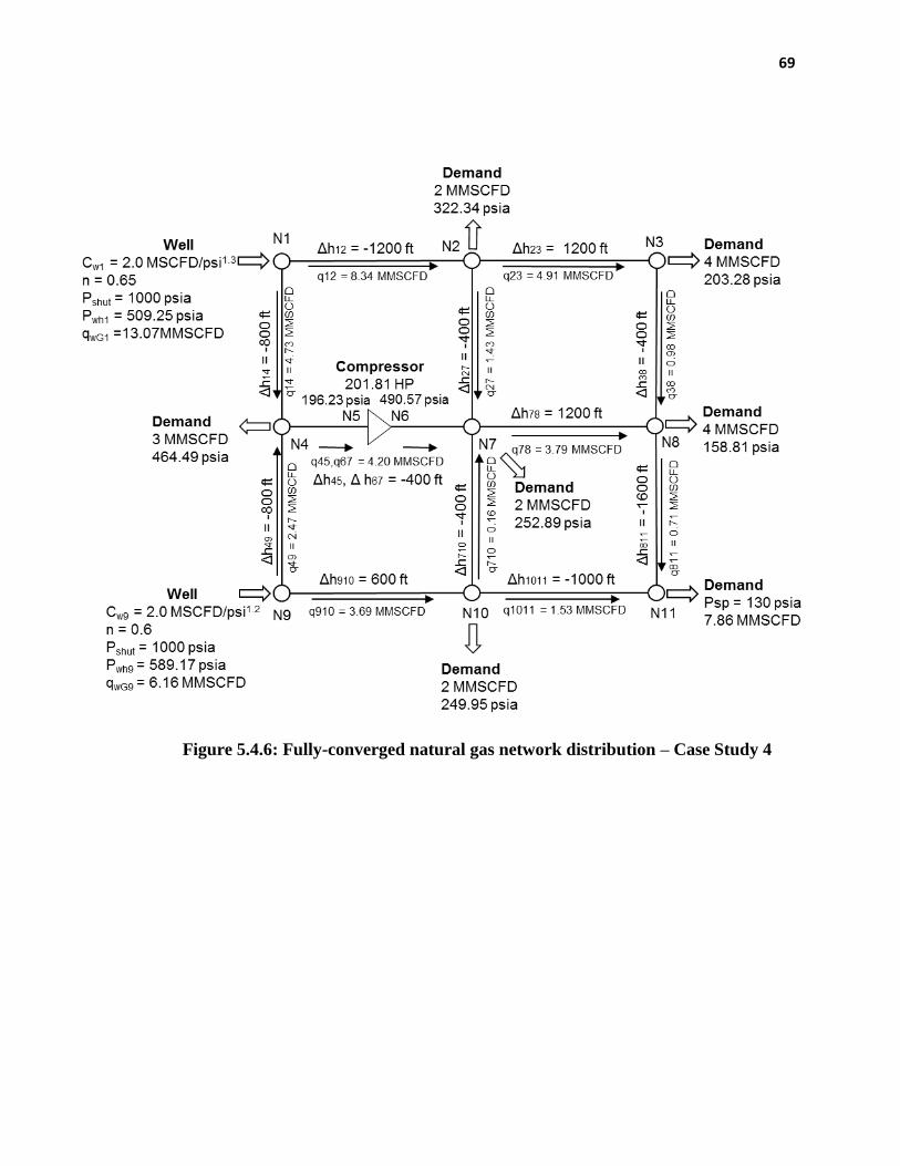
69

Figure 5.4.6: Fully-converged natural gas network distribution – Case Study 4

70

5.5 Case Study 5: Mexico Valley Field Case

Figure 5.5 Network Topology of Mexico Valley

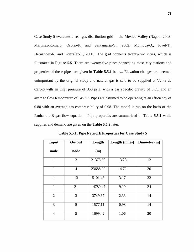
71

Case Study 5 evaluates a real gas distribution grid in the Mexico Valley (Nagoo, 2003;

Martinez-Romero, Osorio-P, and Santamaria-V., 2002; Montoya-O., Jovel-T.,

Hernandez-R, and Gonzalez-R, 2000). The grid connects twenty-two cities, which is

illustrated in Figure 5.5. There are twenty-five pipes connecting these city stations and

properties of these pipes are given in Table 5.5.1 below. Elevation changes are deemed

unimportant by the original study and natural gas is said to be supplied at Venta de

Carpio with an inlet pressure of 350 psia, with a gas specific gravity of 0.65, and an

average flow temperature of 345 ºR. Pipes are assumed to be operating at an efficiency of

0.80 with an average gas compressibility of 0.98. The model is run on the basis of the

Panhandle-B gas flow equation. Pipe properties are summarized in Table 5.5.1 while

supplies and demand are given on the Table 5.5.2 later.

Table 5.5.1: Pipe Network Properties for Case Study 5

Input

node

Output

node

Length

(m)

Length (miles) Diameter (in)

1 2 21375.50 13.28 12

1 4 23688.90 14.72 20

1 13 5101.48 3.17 22

1 21 14789.47 9.19 24

2 3 3749.67 2.33 14

3 5 1577.11 0.98 14

4 5 1699.42 1.06 20

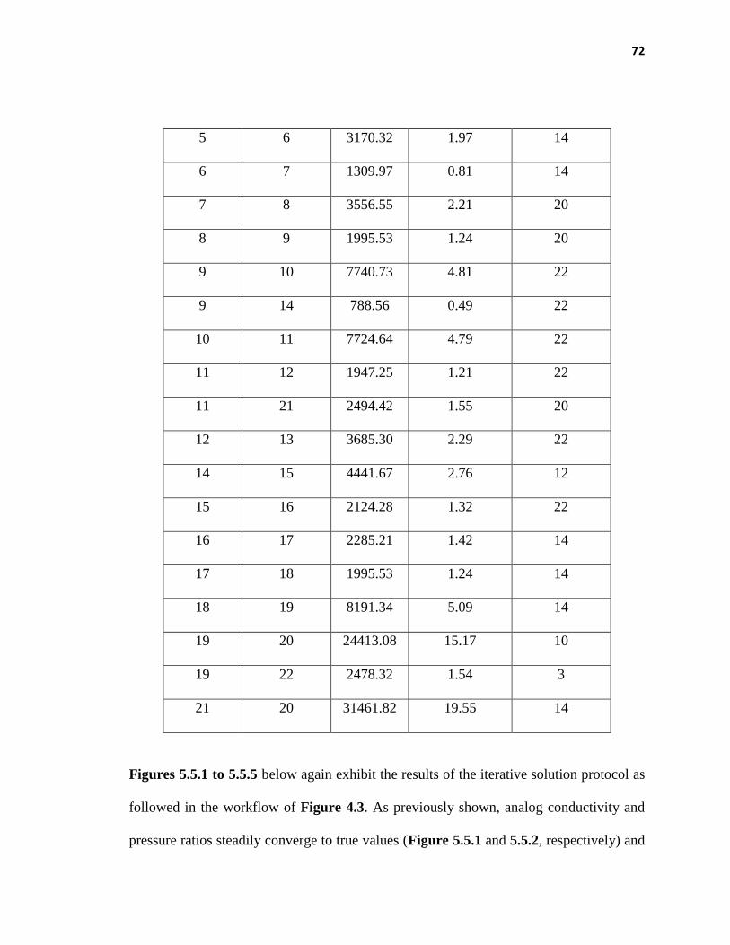
72

5 6 3170.32 1.97 14

6 7 1309.97 0.81 14

7 8 3556.55 2.21 20

8 9 1995.53 1.24 20

9 10 7740.73 4.81 22

9 14 788.56 0.49 22

10 11 7724.64 4.79 22

11 12 1947.25 1.21 22

11 21 2494.42 1.55 20

12 13 3685.30 2.29 22

14 15 4441.67 2.76 12

15 16 2124.28 1.32 22

16 17 2285.21 1.42 14

17 18 1995.53 1.24 14

18 19 8191.34 5.09 14

19 20 24413.08 15.17 10

19 22 2478.32 1.54 3

21 20 31461.82 19.55 14

Figures 5.5.1 to 5.5.5 below again exhibit the results of the iterative solution protocol as

followed in the workflow of Figure 4.3. As previously shown, analog conductivity and

pressure ratios steadily converge to true values (Figure 5.5.1 and 5.5.2, respectively) and

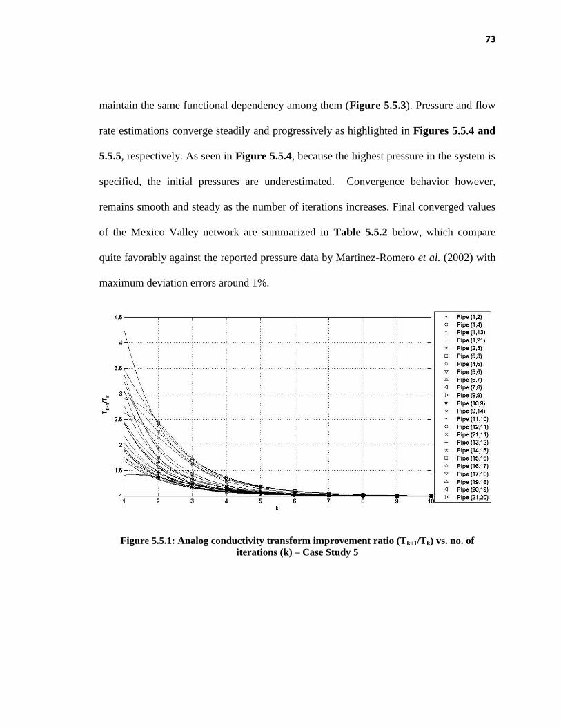
73

maintain the same functional dependency among them (Figure 5.5.3). Pressure and flow

rate estimations converge steadily and progressively as highlighted in Figures 5.5.4 and

5.5.5, respectively. As seen in Figure 5.5.4, because the highest pressure in the system is

specified, the initial pressures are underestimated. Convergence behavior however,

remains smooth and steady as the number of iterations increases. Final converged values

of the Mexico Valley network are summarized in Table 5.5.2 below, which compare

quite favorably against the reported pressure data by Martinez-Romero et al. (2002) with

maximum deviation errors around 1%.

Figure 5.5.1: Analog conductivity transform improvement ratio (Tk+1/Tk) vs. no. of

iterations (k) – Case Study 5

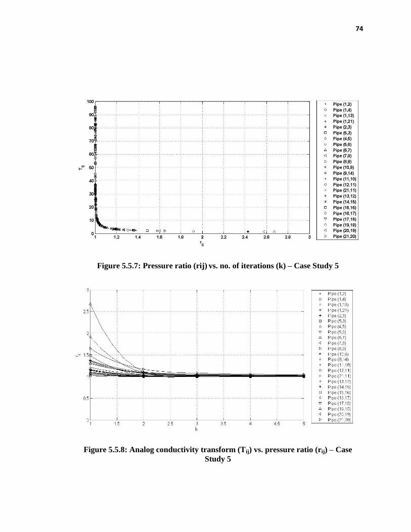
74

Figure 5.5.7: Pressure ratio (rij) vs. no. of iterations (k) – Case Study 5

Figure 5.5.8: Analog conductivity transform (Tij) vs. pressure ratio (rij) – Case

Study 5

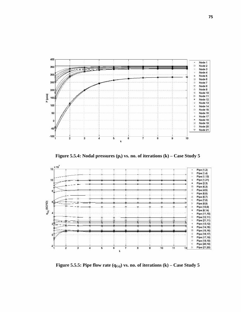
75

Figure 5.5.4: Nodal pressures (pi) vs. no. of iterations (k) – Case Study 5

Figure 5.5.5: Pipe flow rate (qGij) vs. no. of iterations (k) – Case Study 5

76

Table 5.5.2: Nodal Network Predictions for Case Study 5

City Node Supply (-) /

Demand (+)

(MMSCFD)

Pressure

reported by

Martinez-

Romero et al.

(psia)

Calculated

Pressure using

Linear Analog

Model (psia)

Deviation

Error (%)

Venta de

Carpio

1 -258.58 356.94 356.94 0.00%

Tultitlán 2 11.79 345.77 346.33 0.16%

Lechería 3 14.04 345.77 346.24 0.14%

Yets 4 0.00 346.49 347.00 0.15%

Barrientos 5 0.00 345.77 346.31 0.16%

Anahuac 6 18.96 340.26 340.42 0.05%

Romana 7 15.79 339.39 339.48 0.03%

Comunidad 8 9.58 339.24 339.37 0.04%

Río de los 9 0.00 339.24 339.36 0.03%

San Juanico 10 17.46 344.32 344.36 0.01%

Cerro Gordo 11 13.92 351.28 351.28 0.00%

Tulpetlac 12 6.29 351.86 351.88 0.01%

Sosa

Texcoco

13 27.75 353.31 353.27 -0.01%

Vallejo 14 16.92 338.66 338.80 0.04%

18 de Marzo 15 55.63 289.49 286.58 -1.01%

Camarones 16 9.17 289.35 286.45 -1.00%

Anahuac 78 17 10.33 288.77 285.86 -1.01%

Anahuac 80 18 14.46 288.63 285.77 -0.99%

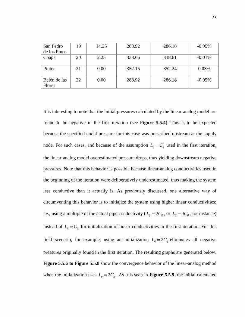
77

San Pedro

de los Pinos

19 14.25 288.92 286.18 -0.95%

Coapa 20 2.25 338.66 338.61 -0.01%

Pinter 21 0.00 352.15 352.24 0.03%

Belén de las

Flores

22 0.00 288.92 286.18 -0.95%

It is interesting to note that the initial pressures calculated by the linear-analog model are

found to be negative in the first iteration (see Figure 5.5.4). This is to be expected

because the specified nodal pressure for this case was prescribed upstream at the supply

node. For such cases, and because of the assumption ij ijL C used in the first iteration,

the linear-analog model overestimated pressure drops, thus yielding downstream negative

pressures. Note that this behavior is possible because linear-analog conductivities used in

the beginning of the iteration were deliberatively underestimated, thus making the system

less conductive than it actually is. As previously discussed, one alternative way of

circumventing this behavior is to initialize the system using higher linear conductivities;

i.e., using a multiple of the actual pipe conductivity ( 2ij ijL C , or 3ij ijL C , for instance)

instead of ij ijL C for initialization of linear conductivities in the first iteration. For this

field scenario, for example, using an initialization 2ij ijL C eliminates all negative

pressures originally found in the first iteration. The resulting graphs are generated below.

Figure 5.5.6 to Figure 5.5.8 show the convergence behavior of the linear-analog method

when the initialization uses 2ij ijL C . As it is seen in Figure 5.5.9, the initial calculated

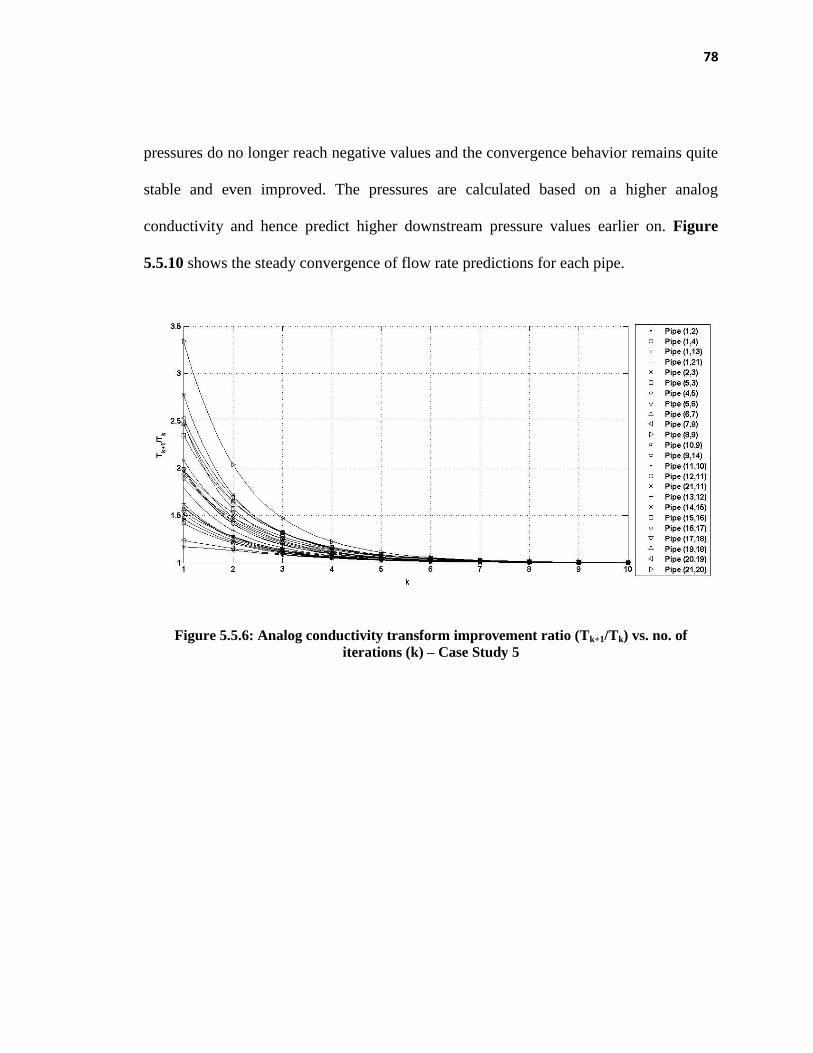
78

pressures do no longer reach negative values and the convergence behavior remains quite

stable and even improved. The pressures are calculated based on a higher analog

conductivity and hence predict higher downstream pressure values earlier on. Figure

5.5.10 shows the steady convergence of flow rate predictions for each pipe.

Figure 5.5.6: Analog conductivity transform improvement ratio (Tk+1/Tk) vs. no. of

iterations (k) – Case Study 5

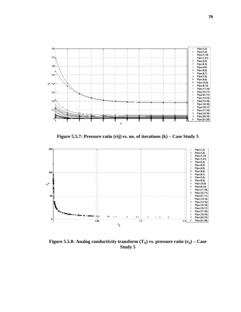
79

Figure 5.5.7: Pressure ratio (rij) vs. no. of iterations (k) – Case Study 5

Figure 5.5.8: Analog conductivity transform (Tij) vs. pressure ratio (rij) – Case

Study 5

80

Figure 5.5.9: Nodal pressures (pi) vs. no. of iterations (k) – Case Study 5

Figure 5.5.10: Pipe flow rate (qGij) vs. no. of iterations (k) – Case Study 5

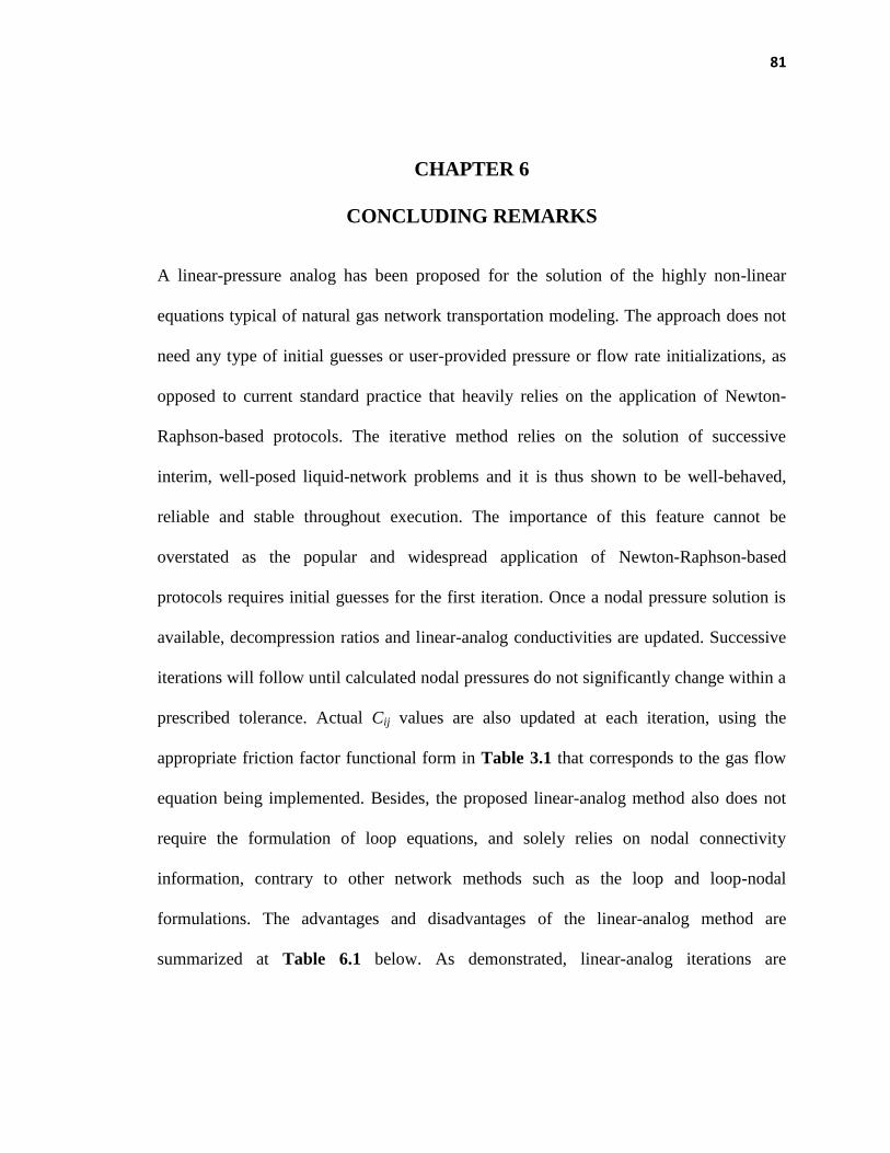
81

CHAPTER 6

CONCLUDING REMARKS

A linear-pressure analog has been proposed for the solution of the highly non-linear

equations typical of natural gas network transportation modeling. The approach does not

need any type of initial guesses or user-provided pressure or flow rate initializations, as

opposed to current standard practice that heavily relies on the application of Newton-

Raphson-based protocols. The iterative method relies on the solution of successive

interim, well-posed liquid-network problems and it is thus shown to be well-behaved,

reliable and stable throughout execution. The importance of this feature cannot be

overstated as the popular and widespread application of Newton-Raphson-based

protocols requires initial guesses for the first iteration. Once a nodal pressure solution is

available, decompression ratios and linear-analog conductivities are updated. Successive

iterations will follow until calculated nodal pressures do not significantly change within a

prescribed tolerance. Actual Cij values are also updated at each iteration, using the

appropriate friction factor functional form in Table 3.1 that corresponds to the gas flow

equation being implemented. Besides, the proposed linear-analog method also does not

require the formulation of loop equations, and solely relies on nodal connectivity

information, contrary to other network methods such as the loop and loop-nodal

formulations. The advantages and disadvantages of the linear-analog method are

summarized at Table 6.1 below. As demonstrated, linear-analog iterations are

82

inexpensive in both implementation and execution when compared to Newton-Raphson

iterations because they do not rely on Jacobian or derivative calculations.

Essentially, the linear-analog method presented is able to solve gas load flow problems

for any fluid system without the need for heavy computational power. The method

successfully preserves all the advantages of the Newton-nodal method while truncating

the need for initial guesses and, at the same time, it also eliminates the needs for Jacobian

formulations and calculation of derivatives. However, a potential drawback of the

proposed method is that its convergence is non-quadratic and more analog iterations may

be required for final convergence once the iterative solution gets close to the actual

solution. For iterative solutions that are close to the actual solution, Newton-Raphson

protocols could become more efficient once initialized using linear-analog-generated

initial values. A hybrid approach can be devised where the linear-analog method is first

implemented to inexpensively and reliably advance the network solution up to a point

where the quadratic convergence of the nodal Newton-Raphson protocol can be fully

taken advantage of without diverging hopelessly.

Subsequently, a wider range of pipeline network system analyses could then be executed

with ease. One of the most important applications of pipe network analysis, such as the

one applied to the system in Figure 1.1, is its ability to carry out network-wide sensitivity

analysis. Sensitivity analysis is used to prioritize what changes in network components

are the most important for the improvement of overall network performance. This can be

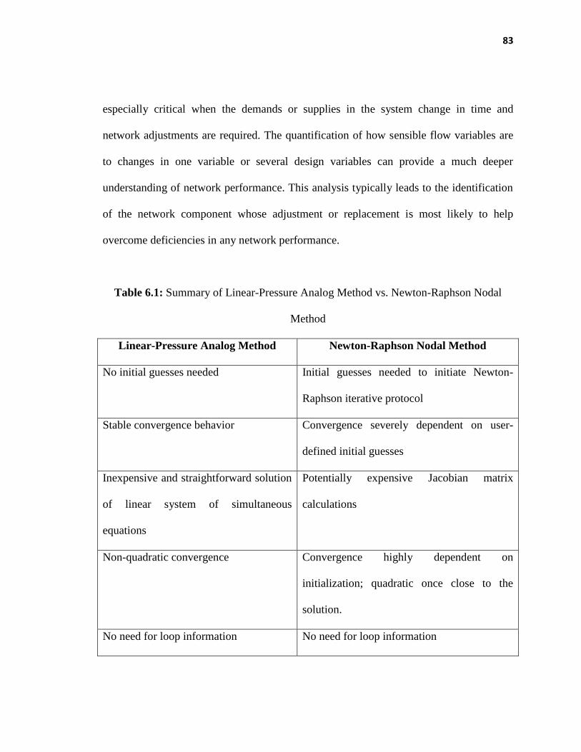
83

especially critical when the demands or supplies in the system change in time and

network adjustments are required. The quantification of how sensible flow variables are

to changes in one variable or several design variables can provide a much deeper

understanding of network performance. This analysis typically leads to the identification

of the network component whose adjustment or replacement is most likely to help

overcome deficiencies in any network performance.

Table 6.1: Summary of Linear-Pressure Analog Method vs. Newton-Raphson Nodal

Method

Linear-Pressure Analog Method Newton-Raphson Nodal Method

No initial guesses needed Initial guesses needed to initiate Newton-

Raphson iterative protocol

Stable convergence behavior Convergence severely dependent on user-

defined initial guesses

Inexpensive and straightforward solution

of linear system of simultaneous

equations

Potentially expensive Jacobian matrix

calculations

Non-quadratic convergence Convergence highly dependent on

initialization; quadratic once close to the

solution.

No need for loop information No need for loop information

84

BIBLIOGRAPHY

Ayala, L. F. (2012). Chapter 21: Transportation of Crude Oil, Natural Gas, and Petroleum

Products. ASTM Handbook of Petroleum and Natural Gas Refining and

Processing. ASTM International.

Boyd, O. W. (1983). Petroleum Fluid Systems. Norman: Campbell Petroleum Series.

Brebbia, C. A., and Ferrante, A. J. (1983). Computational Hydraulics. Butterworth-

Heinemann Ltd.

Crafton, J. W. (1976, October 3-6). An Iterative Solution for the Gas Pipeline Network

Problem. SPE 6032. Dallas, Texas, United States of America: Society of

Petroleum Engineers Journal.

Cross, H. (1932). Analysis of Continuous Frames by Distributing Fixed-End Moments.

Transactions of ASCE, v 96, n 1793, 1-10.

Dranchuk, P. M., and Abou-Kassem, J. H. (1975). Calculation of Z Factors For Natural

Gases Using Equations of State. Journal of Canadian Petroleum Technology, 34-

36.

Golan, M., and Whitson, C. H. (1991). Well Performance. Englewood Cliffs: Prentice

Hall.

Ikoku, C. U. (1984). Natural Gas Production Engineering. New York: John Wiley and

Sons.

Johnson, T. W., and Berwald, W. B. (1935). Flow of Natural Gas Through High-

Pressure Transmission Lines. U.S. Department of the Interior Bureau of Mines.

Larock, B. E., Jeppson, R. W., and Watters, G. Z. (1999). Hydraulics of Pipeline Systems.

CRC Press.

Li, Q., An, S., and Gedra, T. W. (2003). Solving Natural Gas Loadflow Problems Using

Electric Loadflow Techniques. Stillwater.

Mageid, H. A., Hago, A. W., and Magid, I. A. (1991). Analysis of Pipe Networks by the

Finite Element Method. Water International, Vol. 16, Iss. 2.

85

Martinez-Romero, N., Osorio-P, O., and Santamaria-V., I. (2002). Natural Gas Network

Optimization and Sensibility Analysis. SPE Paper 74384. Society of Petroleum

Engineers.

Menon, E. (2005). Gas Pipeline Hydraulics. Boca Raton: CRC Press Taylor and Francis

Group.

Mohitpour, M., Golshan, H., and Murray, A. (2007). Pipeline Design and Construction.

New York: ASME Press.

Montoya-O., S. J., Jovel-T., W. A., Hernandez-R, J. A., and Gonzalez-R, C. (2000).

Genetic Algorithms Applied to the Optimum Design of Gas Transmission

Networks. SPE 59030. Society of Petroleum Engineers.

Murphy, H. G. (1989, October 19-20). Compressor Performance Modeling to Improve

Efficiency and the Quality of The Optimization Decisions. PSIG. El Paso, Texas,

United States of America: Pipeline Simulation Interest Group.

Nagoo, A. S. (2003, August). Analysis of Steady and Quasi-Steady Gas Flows in

Complex Pipe Network Topology. PA, United States of America: The

Pennsylvania State University Graduate School.

Osiadacz, A. J. (1987). Simulation And Analysis of Gas Networks. Houston: Gulf

Publishing Company.

Press, W. H., Teukolsky, S. A., Vetterling, W. T., and Flannery, B. P. (2002). Numerical

Recipes in C++: The Art of Scientific Computing Second Edition. New York:

Cambridge University Press.

Rawlins, E. L., and Schellhardt, M. A. (1936). Back-Pressure Data on Natural Gas Wells

and Their Application to Production Practices. U.S. Bureau of Mines Monograph

7.

Schroeder, D. W. (2011, August 16). A Tutorial on Pipe Flow Equations. Carlisle,

Pennsylvania: Stoner Associates, Inc.

Sutton, R. P. (1985). Compressibility Factors for High-Molecular-Weight Reservoir

Gases. SPE 14265. Las Vegas, Nevada, USA: SPE.

Weymouth, T. R. (1912). Problems in Natural Gas Engineering. Transactions of ASME v.

34, 185-206.

86

Wood, D., and Carl, O.A , Hydraulic Network Analysis Using Linear Theory, Journal of

the Hydraulics Division, ASCE, vol. 98, No. 7, July, pp. 1157-1170, 1972.

Zhou, J., and Adewumi, M. A. (1998, November 9-11). Gas Pipeline Network Analysis

Using an Analytical Steady-State Flow Equation. SPE 51044. Pittsburgh, PA,

United States of America: Society of Petroleum Engineers.

87

APPENDIX

The model in this thesis was developed using two separate programs. The input data will

be read and manipulated on an Excel Spreadsheet. Users will have to have Microsoft

Excel installed on their computer platforms. On the other hand, the algorithm for the

model is done in MATLAB by MathWorks. The Appendix will explain the algorithm

behind the codes and how users could implement that for each case study presented here.

A1 – Input Data for Case Study

Solution Method [1, 2] is where users select 1 for solving the system with Linear Analog

Method or 2 for solving with Newton-Raphson procedure.

Pipe Equation [1, 2, 3, 4, 5] is where users select 1 for Generalized Flow Equation, 2 for

Weymouth friction Factor, 3 for Pandhandle-A, 4 for Panhandle-B and 5 for Fully

Turbulent AGA.

The program requires the users to input the gas properties where:

Average Temperature [Value] is where users input the average gas temperature in

Rankine.

Solution Method 1

Pipe Equation 5

Gas Properties

Average Temperature (R) 535

Specific Gravity 0.69

Compressibility Factor 0.9

GasNet v1.0

by Chew Y. Leong

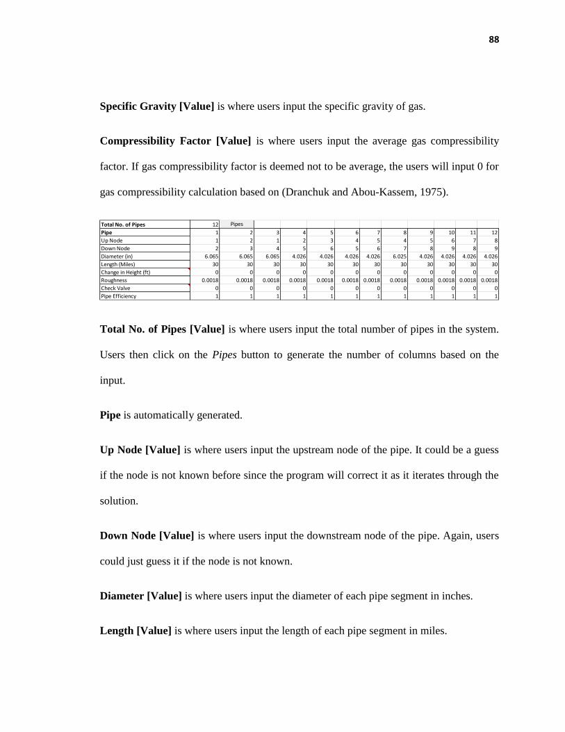
88

Specific Gravity [Value] is where users input the specific gravity of gas.

Compressibility Factor [Value] is where users input the average gas compressibility

factor. If gas compressibility factor is deemed not to be average, the users will input 0 for

gas compressibility calculation based on (Dranchuk and Abou-Kassem, 1975).

Total No. of Pipes [Value] is where users input the total number of pipes in the system.

Users then click on the Pipes button to generate the number of columns based on the

input.

Pipe is automatically generated.

Up Node [Value] is where users input the upstream node of the pipe. It could be a guess

if the node is not known before since the program will correct it as it iterates through the

solution.

Down Node [Value] is where users input the downstream node of the pipe. Again, users

could just guess it if the node is not known.

Diameter [Value] is where users input the diameter of each pipe segment in inches.

Length [Value] is where users input the length of each pipe segment in miles.

Total No. of Pipes 12

Pipe 1 2 3 4 5 6 7 8 9 10 11 12

Up Node 1 2 1 2 3 4 5 4 5 6 7 8

Down Node 2 3 4 5 6 5 6 7 8 9 8 9

Diameter (in) 6.065 6.065 6.065 4.026 4.026 4.026 4.026 6.025 4.026 4.026 4.026 4.026

Length (Miles) 30 30 30 30 30 30 30 30 30 30 30 30

Change in Height (ft) 0 0 0 0 0 0 0 0 0 0 0 0

Roughness 0.0018 0.0018 0.0018 0.0018 0.0018 0.0018 0.0018 0.0018 0.0018 0.0018 0.0018 0.0018

Check Valve 0 0 0 0 0 0 0 0 0 0 0 0

Pipe Efficiency 1 1 1 1 1 1 1 1 1 1 1 1

Pipes

89

Change in Height [Value] is where users input the elevation in term of feets for each

pipe segment measured from the base datum.

Roughness [Value] is where users input the roughness factor of the pipe segment.

Check Valve [1, 0] is where users select 1 if check valve is installed on pipe to avoid

backflow and 0 if there is no check valve installed.

Pipe Efficiency [Value] is where the users input the efficiency of the pipe for calibration

purposes.

Total No. of Nodes [Value] is where users input the total number of nodes in the system.

Users then press Nodes button to generate the specified number of nodes.

Node is automatically generated.

Supply [-] / Demand [+] [Value] is where users input the supply and demand of each

node in terms of MMSCFD.

Initial Pressure Guess is only applicable when users select Newton-Raphson procedure

for solving the system.

Total No. of Nodes 9

Node 1 2 3 4 5 6 7 8 9

Supply [-] /Demand [+] (MMSCFD) -16 2 2 3 1 2 2 2 2

Initial Pressure Guess

Nodes

Total No. of Specified Nodes 1

Node with Specified Pressure 9

Specified Pressure (Psia) 130

Sp. Nodes

90

Total No. of Specified Nodes [Value] is where users input the total number of specified

nodes in the system. Users then click on Sp. Nodes button to generate the columns

according to the total number.

Node with Specified Pressure [Value] is where users input the location of the specified

nodes. Caution: users want to make sure that whenever possible the node with lowest

pressure should be specified to avoid overestimating the lowest pressure. Users should

also specify exit nodes when there are wells since the total demand of the system is

unknown.

Total No. of Wellheads [Value] is where users input the total number of wellheads of

the system. Users should then click Wells button to generate the columns needed for data

input.

Node as Wells [Value] is where users input the location of the well according to the

nodes.

Well Conductivity [Value] is where users input the data for Cw for each well in units of

(MMSCFD/psia)

Shut-In Pressure [Value] is where users input the data for the shut-in pressure of the

well in terms of Psia.

Total No. of Wellheads 0

Node as Wells

Well Conductivity (MMSCFD/psia)

Shut-In Pressure (Psia)

Flow Exponent

Wells

91

Flow Exponent [0.5-1] is where users input the data for the flow exponent of the

particular well.

Total No. of Compressors [Value] is where users input the data for the total number of

compressors in the system. Users then click on Compressors button to generate the

number of columns according to the total number.

Compressors are automatically generated.

Up Node [Value] is where users input the upstream node of the compressor.

Down Node [Value] is where users input the downstream node of the compressor.

Specific Heats of Gas [Value] is where users input the specific heats of gas or polytropic

exponent in polytropic process.

Adiabatic Efficiency [Value] is where users input the value of the efficiency of the

compressor.

Suction Temperature [Value] is where users input the value of the suction temperature

for the gas in Rankine.

Total No. of Compressors 0

Compressors

Up Node

Down Node

Specific Heats of Gas [γ]

Adiabatic Efficiency

Suction Temperature (R)

Compressor Ratio Specified

Horsepower Specified (HP)

Compressors

92

Compressor Ratio Specified [Value] is where users input the value of compression ratio

for the compressor. It is only applicable if the users are selecting Linear-Analog method

as the model.

Horsepower Specified [Value] is where users input the value of horsepower of the

compressor in terms of HP. It is only applicable if the users are selecting Newton-

Raphson method for the solution model.

93

A2 – Linear-Analog Algorithm

The implementation of the linear-analog method relies fundamentally on the way users

define their system since network could be expressed in incidence matrix. The code

snippets below show how the matrix could be formed. The program below is written in

MATLAB coding language.

In order to form the characteristic matrix K, the upper and lower matrixes are first formed

with the codes above. It then checks if compressor is included in the system and

compressors constants are included in the characteristic matrix K.

%Initializing matrix

matrix=zeros(nodes_no);

residual=zeros(nodes_no,1); %Forming upper and lower matrix

for ii=1:pipes_no

matrix(up_node(ii),dn_node(ii))=C(ii);

matrix(dn_node(ii),up_node(ii))=C(ii);

if abs(s(ii))>0

matrix(up_node(ii),dn_node(ii))=exp(s(ii)/2)*matrix(up_node(ii),dn_node(ii));

end

end

%Including Compressors

if comp_no~=0

for ii=1:comp_no

matrix(comp_upnode(ii),comp_dnnode(ii))=-Cc(ii);

for jj=1:pipes_no

if up_node(jj)==comp_dnnode(ii)

matrix(comp_dnnode(ii),comp_upnode(ii))=-compratio(ii)*C(jj);

matrix(dn_node(jj),up_node(jj))=0;

matrix(dn_node(jj),comp_upnode(ii))=compratio(ii)*C(jj);

end

end

end

end

94

The diagonal entries, Oi and the residual vector or the network consumption/demand

vector, P are then formulated according to the algorithm listed above.

%Forming Diagonal Entries

%Forming Residual Vector

column=1; %Including Pipes

for row=1:nodes_no

for loop=1:pipes_no

if up_node(loop)==row

matrix(row,column)=-C(loop)+matrix(row,column);

end

if abs(s(loop))>0 andand dn_node(loop)==row

matrix(row,column)=-exp(s(loop)/2)*(C(loop))+matrix(row,column);

elseif dn_node(loop)==row

matrix(row,column)=-C(loop)+matrix(row,column);

end

end

residual(row)=supply_demand(row)*10^6+residual(row); %Including Wells

if wells_no~=0

for loop=1:wells_no

if row==wells(loop)

matrix(row,column)=-wellc(loop)+matrix(row,column);

residual(wells(loop))=-wellc(loop)*Pshut(loop)+residual(wells(loop));

end

end

end

%Including Compressors

if comp_no~=0

for cloop=1:comp_no

if comp_dnnode(cloop)==row

matrix(row,column)=Cc(cloop);

end

end

end

95

Nodes with specified pressures are then substituted in the network consumption/demand

vector, P and if there is compressor, the pressure is updated with the compression ratio

and calculated upstream node pressure.

%Including Specified Nodes

for i=1:spnodes_no

if row==nsp(i)

matrix(row,:)=0;

matrix(row,column)=1;

end

end

column=column+1;

end

%Including Specified Nodes in Residual

for i=1:spnodes_no

residual(nsp(i))=sp_pressure(i);

end

%Shutting Node to prevent backflow if check valve is installed

for i=1:nodes_no

if off(i)==1

residual(i)=pressure(dn_node(i));

matrix(i,i)=1;

end

end

%Calculating New Pressures

pressure_old=pressure;

pressure=matrix\residual; %Calculate HP

if comp_no~=0

for i=1:comp_no

HP(i)=pressure(comp_dnnode(i));

pressure(comp_dnnode(i))=compratio(i)*pressure(comp_upnode(i));

end

end