a review of methods for constrained eigenvalue...
TRANSCRIPT

A Review of Methods for ConstrainedEigenvalue Problems
J.G.M. Kerstens
Technical University Eindhoven, PO Box 513, 5600 AB Eindhoven, The Netherlands
Numerous studies are concerned with vibrations or buckling of constrained systems realising that
complex systems can be analysed when starting from unconstrained or known problems.
Over the years various constrained eigenvalue formulations have been published and put into
practical use. The most important ones are the Lagrangian multiplier method (modal synthesis
method or component modes synthesis method), the receptance method and the modal constraint
method. In this paper the similarities and merits of the various methods are discussed.
It is striking that so far the similarities of the various constrained eigenvalue expressions have not
been reported nor has the similarity of the eigenvalue expressions of these methods with
Weinstein’s determinant for intermediate problems of the first type been noticed.
The eigenvalue formulations of the Lagrangian multiplier method and that of the receptance
appear to be similar to Weinstein’s determinant for intermediate problems of the first type. The
modal constraint method is based on an extension of Weinstein’s method for intermediate
problems of the first type and offers some significant advantages, i.e. the resulting eigenvalue
formulation of the modal constraint method has a standard form in contrast with that of the other
mentioned methods in that they have the known and unknown eigenvalues in the denominator of
the eigenvalue formulations. Further, zero modal displacements, persistent and multiple
eigenvalues do require special attention using these methods whereas this is not the case for the
modal constraint method.
Based on the similarities of the various constrained eigenvalue expressions a number of
interesting conclusions are drawn.
Keywords: vibration, buckling, constraints, component mode synthesis, modal synthesis method,
receptance method, modal constraint method.
1 Introduction
There are a number of methods that deal with the problem of constrained vibrations, i.e. the
vibrations of constrained linear mechanical systems.
The eigenvalue equations of these methods, notably the receptance method [5] and the
Lagrangian multiplier method [6] do not allow persistent eigenvalues readily to be calculated,
i.e. eigenvalues common to both the unconstrained and the constrained problem to be
computed. This rule and the resulting eigenvalue equations of these methods do not allow the
109HERON, Vol. 50, No 2 (2005)
use of standard numerical eigenvalue solvers. Here root finding procedures like the bi-section
methods have to be applied. However persistent and multiple eigenvalues cannot be calculated
using these methods. Some possible approaches to tackle these problems will be discussed.
Furthermore, the eigenfunctions, i.e. the Lagrangian multipliers or receptances of these
eigenvalue formulations do not directly allow constrained mode shapes to be evaluated.
Notwithstanding these observations, the Lagrangian method [11-17] and the receptance method
[18-23] are widely used without realising that both methods appear to be in essence similar.
The modal constraint method has been developed starting from Weinstein’s determinant of the
first type and does not suffer from the abovementioned drawbacks [7-10].
There is a need to discuss the similarities, differences, merits and demerits of the various
methods for constrained eigenvalue problems.
In section 2 the basics of the Lagrangian method will be presented resulting in an constrained
eigenvalue expression. The drawbacks of this method will be summarised. Also the
boundedness of eigenvalues is discussed.
Thereafter in section 3 the receptance method will be discussed. The constrained eigenvalue
expression is similar to the one for the Lagrangian multiplier method altough both methods
depart from entirely different approaches.
Then, in section 4 Weinstein’s method of intermediate problems of the first type will be treated.
It will be shown that the Lagrangian multiplier method and the receptance method that deal
with constrained vibrating problems are in fact similar to Weinstein’s method of the first type,
i.e. their eigenvalue formulations have similar formulations. Weinstein’s method is firmly based
on the principles of differential operators and presents a stepping stone in the proof of the
observed boundedness of constrained eigenvalues.
Weinstein’s theory is based on arbitrary constraint functions. In section 5 a particular choice for
these constraint functions will be given that relates to physical constraint conditions such as
point supports.
Thereafter, in section 6 the modal constraint method based on a differential operator basis will
be presented which allow persistent eigenvalues and also mode shapes to be established. Here
it will be demonstrated how Lagrangian multipliers can be expanded into known quantities,
which is the essence of the modal constraint method.
In section 7 the modal constraint method is treated in terms of energy functionals. It appears
that the Lagrangian multipliers can be identified as the inner product of the constrained
operator and the constraint functions.
In section 8 the similarities, differences, merits and demerits of constrained eigenvalue
problems are summarised.
110

2 The Lagrangian Multiplier Method
2.1 Introduction
The treatment of the Lagrangian multiplier method by Dowell [6] has been inspired by the
early work of Budianski and Hu [4]. The latter author treat buckling problems for constrained
structures using Lagrangian multipliers. He also realised that this method can also be applied
to free vibration problems.
The free vibrations of an arbitrary structure in terms of component modes are determined by
the use of normal modes of an unconstrained structure.
This is achieved by enforcing continuity conditions using Lagrangian multipliers. Dowell
regards the method as a constrained Rayleigh-Ritz method with constraint or continuity
conditions.
It is well known that the Rayleigh-Ritz method provides upper bounds for the eigenvalues.
From the results published it can be concluded that the Lagrangian multiplier method also
referred to in the literature as component mode synthesis method or modal synthesis method
provides upper bounds for a fixed number of constraints and lower bounds for a fixed number
of component modes.
2.2 Presentation of the method
In order to derive the Lagrangian equations of motion first the potential and the kinetic energy
expressions are given. For sufficiently small values of the generalised velocities the kinetic
energy may be approximated by
(1)
where M ij
is the generalised mass coefficient and
(2)
If the generalised coordinates qiare also small the potential energy can be approximated by
(3)
where K ij
is the generalised stiffness coefficient.
Dowell assumes k constraint conditions in the following form
U q q Ki j ijj
n
i
n
===∑∑1
2 11
tii=
∂∂
T q q Mi jj
n
i
n
ij===∑∑1
2 11
� �
�qi
111
(4)
The Lagrangian of the system is then
(5)
where θr
is the Lagrangian multiplier associated with the constraint conditions.
The Lagrangian equations of motion are
(6)
(7)
Expressions (1) and (3) can be simplified if qiare normal coordinates of the unconstrained
system. In this case
(8)
(9)
where δiis the Kronecker delta and ω
i2 are the eigenfrequencies of the unconstrained structure.
With these results the i th equation of motion for the constrained structure becomes
(10)
Let the constrained structure vibrate with a frequency ω , the general coordinates qiand the
Lagrangian multiplier θs
in equation (5) are harmonic functions with frequency ω .
Consequently the amplitude coefficients qican be expressed in terms of the Lagrangian
multipliers θs
by means of equation (5) as follows
M q q ai i i i s sis
k
( )�� + − ==∑ω θ2
1
0
M M i j nij i ij= =δ , , ,..,1
K M i j nij i i ij= =ω δ2 1, , ,..,
∂∂
= =L
r krθ
0 1 2, , ,..,
ddt
Lq
Lq
i ni i
∂∂
−∂∂
= =�
0 1 2, , ,..,
L T U fr rr
k
= − +=∑θ
1
f q a r kr j rjj
n
≡ = ==∑ 0 1 2
1
, , ,...,
112

(11)
Substitution of the above equation into constraint condition (4) gives
(12)
The eigenvalue expression can be written as follows
(13)
Once the eigenvalues of the above equation are known the eigenvectors, i.e. the Lagrangian
multipliers θs
, can be determined.
Substitution of these eigenvectors and associated eigenvalues into equation (4) gives the
generalised qiassociated with the eigenvalues of the constrained problem.
Finally, the mode shapes viof the constrained structure can be determined as follows
(14)
where ujare the mode shapes of the unconstrained or unconstrained structure.
For adding supports to the unconstrained structure then coefficients ari
can be determined as
follows.
Suppose the structure is required to have k point supports, then for a two-dimensional problem
(15)
Comparing the above result with that of equation (4) gives the following identity
Note that the above method can also be applied when several unconstrained structures are
coupled.
a u x yrj j r r≡ ( , )
v x y u x y q r kr r j r r jj
n
( , ) ( , ) , , ,..,= ==∑
1
1 2
v u qi j jj
n
==∑
1
det{( )
}a a
Msi ri
i ii
n
ω ω2 21
0−
==∑
Da a
Mrssi r ri
i ii
n
=−
==∑ θ
ω ω( )2 21
0
qa
Mii
s si
i is
k
=−
==∑ θ
ω ω( ), , ,
2 21
1 2
113

In matrix form equation (13) can be written as follows
or
(16)
2.3 Discussion
The eigenvalue formulation of the Lagrangian multiplier method will present a difficulty when
there is a number of eigenvalues, which are common to both the unconstrained and constrained
problem, i.e. persistent eigenvalues.
As briefly touched on by Dowell [6], the associated elements have to be removed, such as the
associated zero displacements (or rotations) and the persistent eigenvalues.
To solve the eigenvalue equation (16) a dedicated numerical solution procedure is required such
as the root finding procedures like the bi-section methods. However, persistent eigenvalues
stille pose a problem. One way of locating these eigenvalues is to plot the values of the
determinant of equation (16). In cases where infinite values are obtained may point in the
direction of existing persistent eigenvalues. Even when this is successful multiple eigenvalues
cannot be found. Nowhere in the referenced literature these problems have been sufficiently
addressed. Once the eigevalues are established eigenvectors consisting of Lagrangian
multipliers can be obtained. Thereafter, the eigenvectors have to be transferred into
displacement eigenvectors to plot mode shapes and/or to perform dynamic analyses.
Standard numerical eigenvalue solution procedures are only suitable for the following types of
eigenvalue formulations with symmetric matrices
Au - λu = 0
Au - λBu = 0
Another important point that is not mentioned in the vast literature about the component mode
synthesis method is the fact that the column vectors in matrix CT need to be linear independent,
otherwise poor results may be obtained.
CM I
C 01
diag diag
T
( )λθ
−
⎡
⎣⎢⎢
⎤
⎦⎥⎥
=λ
a a
a a
Mn
k kn
11 1
1
1 1
10 0
0 0
0 0
.. . .
.
( )
.
⎡
⎣
⎢⎢⎢
⎤
⎦
⎥⎥⎥
−λ λ
11
11 1
1
M
a a
a a
n n
n
k kn
( )
.. . .
.λ λ−
⎡
⎣
⎢⎢⎢⎢⎢⎢
⎤
⎦
⎥⎥⎥⎥⎥⎥
⎡⎡
⎣
⎢⎢⎢
⎤
⎦
⎥⎥⎥
⎧
⎨⎪
⎩⎪
⎫
⎬⎪
⎭⎪
= ⎨
T
k
θ
θ
1
.
114

Also when constraining points are selected too close to each other the matrix CT may become ill
conditioned.
Note that unlike the modal constraint method (section 6) the columns are not required to be
orthonormal. However an orthonormalisation procedure, like the Gram-Schmidt
orthonormalisation procedure, may point in the direction of ill condition of the constraint
matrix CT .
Finally, it should be noted that the Lagrangian multipliers represent the forces (or moments) of
constraint acting at the point to achieve zero displacements (or rotations). The elements in
equation (16) can be regarded as influence coefficients. It is well known that the Rayleigh-Ritz
method provides upper bounds for the eigenvalues.
From the results obtained it can be concluded that the Lagrangian multiplier method also
referred to in the literature as component mode synthesis method or modal synthesis method
provides upper bounds for a fixed number of constraints and lower bounds for a fixed number
of component modes.
3 The Receptance Method
3.1 Introduction
The method of receptances was developed around 1960 by Bishop and Johnson [5]. This
method enables calculation of the free vibrational characteristics of a combined system from the
characteristics of the component systems.
Wilken and Soedel [23] applied the method to a cylindrical shell with stiffening rings.
The receptance method consists of an evaluation of the responses of the component systems to
forces which vary sinusoidally in time and which are applied at the locations where the
systems are connected.
These responses, due to a set of sinusoidal forces with amplitudes equal to unity, are the so-
called receptances of the component systems. A characteristic feature of the receptance method
is that each component system is treated as a separate vibrating system subjected to the forces
induced by the other component systems.
3.2 Presentation of the receptance method
When sinusoidally varying forces of frequency ω are applied to two linear undamped systems
A and B then
115
(17)
All quantities are functions of the frequency ω . It is assumed that the displacements and forces
of both systems are defined in one global coordinate system. When the two systems are joined
and no external forces are applied to the two systems then
(18)
For the equations (17) and (18) the eigenvalue equation for the combined system is
or
(19)
The values of ω and fA
which are the solutions of above equation are respectively the natural
frequency and the interaction forces mode shapes of the combined system.
The displacement mode shapes can be obtained from equation (17) with ω and fA
as input.
When the system A is only constrained at k points the eigenvalue expression results from
or
(20)
A typical expression for the receptance is
(21)
where based on the notations of the previous section the following identities hold
αφ φ
ω ωrsi r i s
i ii
n x x
M=
−=∑ ( ) ( )
( )2 21
det{ }ααA = 0
x 0 fA A A= = αα
det{ }αα ααA B+ = 0
[ ]αα ααA B A+ =f 0
x x
f fA B
A B
== −
x f
x fA A A
B B B
==
αααα
116

3.3 Discussions
A comparison between the Lagrangian multiplier method and the receptance method leads to
the conclusion that both methods result in identical constrained eigenvalue equations.
Also the so-called influence coefficients in the previous section are receptances as presented
here. The interaction forces are simply the Lagrangian multipliers of the previous section.
From the results obtained it can be concluded that also the receptance method provides upper
bounds for a fixed number of constraints and lower bounds for a fixed number of component
modes.
See section 2.3 for a discussion about the numerical challenges to extract eigenvaleus and mode
shapes when using this method.
4 Weinstein’s Determinant of the first type
4.1 Introduction
In the years 1935-1937 Weinstein [3] introduced a method for obtaining lower bounds of
eigenvalues that is generally called the method of intermediate problems of the first type. Later,
other types of intermediate problems were developed, of which the second type is the most
important one.
The scheme of the intermediate problems is as follows.
Given an eigenvalue problem with operator associated with certain boundary conditions, the
first step is to find a base problem, namely an eigenvalue problem for which the eigenvalues
and eigenfunctions are known. The eigenvalues must be less or equal to the corresponding
eigenvalues of the desired problem.
Then a sequence of intermediate problems can be set up that will link the base problem
(unconstrained problem) to the desired problem (constrained problem) in such a way that the
computed eigenvalues are between those of the base problem and the desired problem.
4.2 Weinstein’s method in its original form (principles)
In this section the Weinstein approach will be briefly given in the form that was applied to a
plate buckling problem [3]. The desired problem consists of a clamped rectangular plate
governed by the following differential equation
Au - λu = ∇2u - λu (22)
φφ
i r ri
i s si
x a
x a
( )
( )
≡≡
117
at boundary C (23)
It is well known that the eigenvalues of Au = λu can also be formulated as the extrema of a
variational problem. It will be demonstrated that, for a variational problem where further
conditions are added, upper bounds for eigenvalues are obtained. This can be achieved by
requiring the function u to lie in a Rayleigh-Ritz manifold of admissible functions.
To find lower bounds, the conditions must be weakened. There is one way of performing this,
namely by constituting a suitable base problem so that each of the eigenvalues is a lower bound
for the corresponding eigenvalues of the desired problem. An infinite sequence of intermediate
problems must be set up to link the base problem eigenvalues to the eigenvalues of the desired
problem as has been already mentioned.
For the clamped plate Weinstein selected a simply supported plate as the base problem for
which exact eigenelements are known.
The limiting case, i.e. the clamped plate, is achieved by applying boundary conditions in the
form of rotational constraints.
4.3 Formulation of the desired problem
Assume that the eigenvalue equation of the desired problem (the given problem) is given by
A(1)u(1) = λu(1) (24)
Operator A(1) has a domain D(1) of the functions u(1) with region R(1) and boundary C(1) .
The eigenvalues are denoted by C(1) and the associated eigenfunctions by ui(1).
When the boundary conditions formed by C(1) are complicated, it could be a difficult task to
find admissible functions.
Suppose, e.g., that eigenvalues for a free-free plate supported also at arbitrarily located points,
are required. To find admissible functions that will vanish at these arbitrary locations is a nearly
impossible task.
Instead of this approach, the method of intermediate problems is applied. In this case a suitable
base problem must be defined, i.e. free-free rectangular plate for which approximate
eigenvalues and eigenfunctions are known.
4.4 Formulation of the base problem
As already indicated in the previous section the desired problem could be solved by using a
different conveniently related problem. In other words, a conveniently shaped region R and
boundary C are selected, assuming that the region R(1) and boundary C(1) are contained in R .
Also an operator A is selected with a domain D for which it is assumed that D(1) is contained, as
a subspace, in D . The domain D consists of functions u defined on R and satisfying C .
uun
=∂∂
= 0
118

It is assumed that the following eigenvalue equation for the base problem is known
Au = λu (25)
The eigenvalues are denoted by λiand the eigenfunctions by u
i, which form a complete
orthonormal set in D .
Hence, every element u in D can be expanded as
(26)
Before the base problem and the desired problem are related the following assumptions have to
be made.
Basic assumptions
1. It is assumed that the functions u(1) lying in space D(1) with region R(1) are defined on the
entire region R, which contains the region R(1) . In other words the eigenfunctions of the
base problem must be capable of describing the eigenfunctions of the desired problem.
This is a very important notion, which also applies to the Lagrangian method and the
receptance method. This has not always been made explicit in literature about these
methods.
2. The functions u(1) in D(1) which are solutions of the desired problem A(1)u(1) = λ(1)u(1) are
restrictions to some set of functions in D with region R to region R(1) . Assume that the
function u in D is required to vanish at k locations. As already shown previously, the
above constraint conditions can be stated as (u,pr)=0 for r=1,2,...,k where p
rare the
constraint functions. These conditions restrict the function u to lie in D(1) .
3. The self-adjoint, positive-definite operator A(1) with domain D(1) is the restriction of the
self-adjoint, positive-definite operator A with domain D to functions in domain D(1). This
restriction is established by the projection operator and is associated with the constraint
functions pr.
4.5 Relation of the desired problem to the base problem
From the basic assumption 1 in the previous section it follows that the functions u(1) in D(1) can
be extended to D by the addition of new functions v in order to form a complete orthonormal
set of functions in D.
Let DΘD(1) represent the infinite dimensional orthogonal complement space to D(1).
Every function u in D can then be uniquely expressed as
u u u u q ui i i ii
n
i
n
= ===∑∑( , )
11
119

u = u(1) + v (27)
where u(1) is in D(1) and v in DΘD(1).
As has already been shown in the preceeding sections it is convenient to introduce a set of
linear independent (orthonormal) constraint functions pr, which span the space DΘD(1).
Also it has been suggested in the previous section that a function in space D be projected onto
the subspace D(1) with the aid of the following projection operator
u(1) = u - Pu (28)
where
(29)
The functions A(1)u(1) can be identified as projections of the functions Au onto the subspace D(1)
orthogonal to DΘD(1) and therefore applying the projection operator to Au gives
A(1)u(1) = Au - PAu (30)
In the earlier section it is also shown that A(1) = QA which constitutes the relation between the
desired operator A(1) and the base operator .
Now with this result the eigenvalue equation for the desired problem can be written as
Au - PAu = λu -λPu (31)
The constraint condition requires u to be orthogonal to the constraint functions Pr
and hence Pu
= 0 , so that the final eigenvalue equation for the desired problem becomes
Au - PAu = λu (32)
4.6 Formulation of a finite sequence of intermediate problems
As already mentioned earlier the infinite dimensional subspace DΘD(1) must be approximated
by successively k intermediate subspaces.
Let Mk
denote the finite dimensional subspace of DΘD(1) spanned by k constraint functions pr
and denote by Dk(1) the infinite dimensional subspace DΘM
kthat approximates the subspace
D(1).
Pu u p p
Pu v
r rr
k
=
==∑( , )
1
120

The following sequence of subspaces can then be set up with the following property
D1(1) ⊃ D
2(1) ⊃ ...... ⊃ D
k(1) ⊃ ...... ⊃ D(1)
(33)
Gould [2] proved that this sequence of subspaces Dk(1) converges for k – ∝ to subspace D(1).
Also the projection of D onto Dk(1) must be truncated
(34)
Therefore the eigenvalue equation for the k th intermediate problem is as follows
Au - PkAu = λu (35)
with eigenvalues and associated eigenfunctions of the k th
intermediate problem.
It can be proved that the eigenvalues converge with increasing k to
respectively since the sequence of subspaces Dk(1) converges to D(1) .
In the next section the Weinstein determinant of the first type will be established for arbitrary
constraint functions.
4.7 The Weinstein determinant and non-persistent eigenvalues
Based on equation (34) the following expression can be written
The desired eigenvalue equation (35) can be written as follows
(36)
where
The scalars αr
are not given scalars but depend on the unknown function u . To establish the
magnitude of αr
, the inner products with ps
are formed, resulting in the following equations
( , ) , , ,....,u p s ks = =0 1 2
Au u p p pk k− = + + +λ α α α1 1 2 2 ....
P Au Au p p p pk r r k kr
k
= = + +=∑( , ) ...α α1 1
1
λ λ11
21( ) ( ), ,.....λ λk k,
( ),
( ), ,....11
21
u uk k,( )
,( ), ,.....1
12
1λ λk k,( )
,( ) .....1
12
1≤ ≤
P u u p pk r rr
k
==∑( , )
1
121
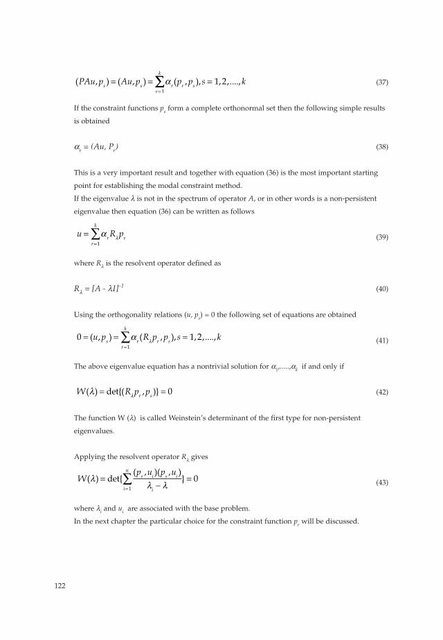
(37)
If the constraint functions ps
form a complete orthonormal set then the following simple results
is obtained
αr
= (Au, Pr) (38)
This is a very important result and together with equation (36) is the most important starting
point for establishing the modal constraint method.
If the eigenvalue λ is not in the spectrum of operator A, or in other words is a non-persistent
eigenvalue then equation (36) can be written as follows
(39)
where Rλ is the resolvent operator defined as
Rλ = [A - λI]-1(40)
Using the orthogonality relations (u, ps) = 0 the following set of equations are obtained
(41)
The above eigenvalue equation has a nontrivial solution for α1,.....,α
kif and only if
(42)
The function W (λ) is called Weinstein’s determinant of the first type for non-persistent
eigenvalues.
Applying the resolvent operator Rλ gives
(43)
where λiand u
iare associated with the base problem.
In the next chapter the particular choice for the constraint function pr
will be discussed.
Wp u p ur i s i
ii
n
( ) det{( , )( , )
}λλ λ
=−
==∑ 0
1
W R p pr s( ) det{( , )}λ λ= = 0
0 1 21
= = ==∑( , ) ( , ), , ,....,u p R p p s ks r r sr
k
α λ
u R pr rr
k
==∑α λ
1
( , ) ( , ) ( , ), , ,....,PAu p Au p p p s ks s r r sr
k
= = ==
α 1 21
∑∑
122

5 The particular choice of constraint functions
5.1 Introductory remarks
In this chapter the particular choice of the constraint functions will be discussed. As already
mentioned these constraint functions are related to the type of constraint. There are three main
types of constraint that can be used, i.e. point supports, line supports and area supports. In this
paper only point supports will be discussed.
A line or area support can be approximated by k point supports that constitute k constraint
functions ps
and therefore a sequence of k intermediate problems.
When expressions for the constraint functions are found for point supports it is possible to
write Weinstein’s equation (43) into an eigenvalue equation for non-persistent eigenvalues for
the desired problem having k points.
After this result this eigenvalue problem is transformed into an eigenvalue equation that will
allow persistent (common to both base and desired problem) eigenvalues, i.e. the modal
constraint method, see section 6.
5.2 Particular choice of constraint functions for adding point supports to the base problem
In practical calculations the complement region R - R(1) and the boundary C(1) may have
complicated shapes and must, therefore, be decomposed into a series of constituents. These
components generate a theoretically infinite chain of constraints of the type given in equation
(44), which must be approximated by a finite number k of these constraints. Therefore, also k
constraint functions ps
exist. The successive application of these k approximating constraint
relations generates what is previously called the k th intermediate problem. In this section, a
particular choice for the constraint functions p1,p
2,...,p
kwill be established, which corresponds to
k constraint conditions.
These constraint or continuity conditions constrain the function u on the region R - R(1) with the
inclusion of boundary C(1), if necessary.
As already discussed these constraints will take the form of an expression between the
generalised coordinates qi
(44)
Taylor expansion about equilibrium, neglecting higher order terms (only small vibrations),
gives the following linear function
(45)
or
h q q qhq
qni
ii
n
( , ,...., ) |1 2 01
0=∂∂
==∑
h q q qn( , ,...., )1 2 0=
123

(46)
If there are k distinct constraint conditions or linear independent constraint relations then k
equations like equation (46) can be set up
(47)
Note that the desired problem has in this case ( n - k ) degrees of freedom and therefore k
eigenvalues equal to zero.
A one-to-one correspondence of equations (47) with constraint functions ps
will be established
using orthogonality condition (u, ps ) = 0 . Because each constraint function p
sis in the space D,
which is spanned by the eigenfunctions ui , the following expansion can be defined
(48)
where bsi
are the expansion coefficients.
Taking the scalar product (u, ps
) = 0 with equation (26) in mind then yields
(49)
Now the one-to-one correspondence between equation (47) and (49) can be observed. Equation
(48) can then be written as
(50)
The finite point set constraint decomposition consists of representing the constraint conditions
for the region R - R(1) and/or boundary C(1) by a finite number of points.
Assume for sake of simplicity a two-dimensional problem where the finite points are located at
coordinates xs, y
s . The function u is required to vanish at each of these points
(51)
If the above equation is compared with equation (49) then the one-to-one correspondence leads
to the following identity
(52)
u x y ci s s si( , ) ≡
u x y u x y q s ks s i s s ii
n
( , ) ( , ) , , ,....,= ==∑ 1 2
1
p c us si ii
n
==∑
1
( , )u p b qs si ii
n
= ==∑ 0
1
p b u s ks si ii
n
= ==∑ , , ,....,1 2
1
h q q q c q l kl n li ii
n
( , ,...., ) , , ,...,1 21
0 1 2= = ==∑
h q q q c qn i ii
n
( , ,...., )1 21
0= ==∑
124
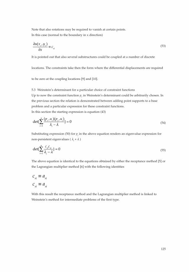
Note that also rotations may be required to vanish at certain points.
In this case (normal to the boundary in x direction)
(53)
It is pointed out that also several substructures could be coupled at a number of discrete
locations. The constraints take then the form where the differential displacements are required
to be zero at the coupling locations [9] and [10].
5.3 Weinstein’s determinant for a particular choice of constraint functions
Up to now the constraint function pr
in Weinstein’s determinant could be arbitrarily chosen. In
the previous section the relation is demonstrated between adding point supports to a base
problem and a particular expression for these constraint functions.
In this section the starting expression is equation (43)
(54)
Substituting expression (50) for pjin the above equation renders an eigenvalue expression for
non-persistent eigenvalues ( λi≠ λ )
(55)
The above equation is identical to the equations obtained by either the receptance method [5] or
the Lagrangian multiplier method [6] with the following identities
With this result the receptance method and the Lagrangian multiplier method is linked to
Weinstein’s method for intermediate problems of the first type.
c a
c ari ri
si si
≡≡
det{ }c cri si
ii
n
λ λ−=
=∑ 0
1
det{( , )( , )
}p u p ur i s i
ii
n
λ λ−=
=∑
1
0
∂∂
≡u x y
xcs s
si
( , )
125
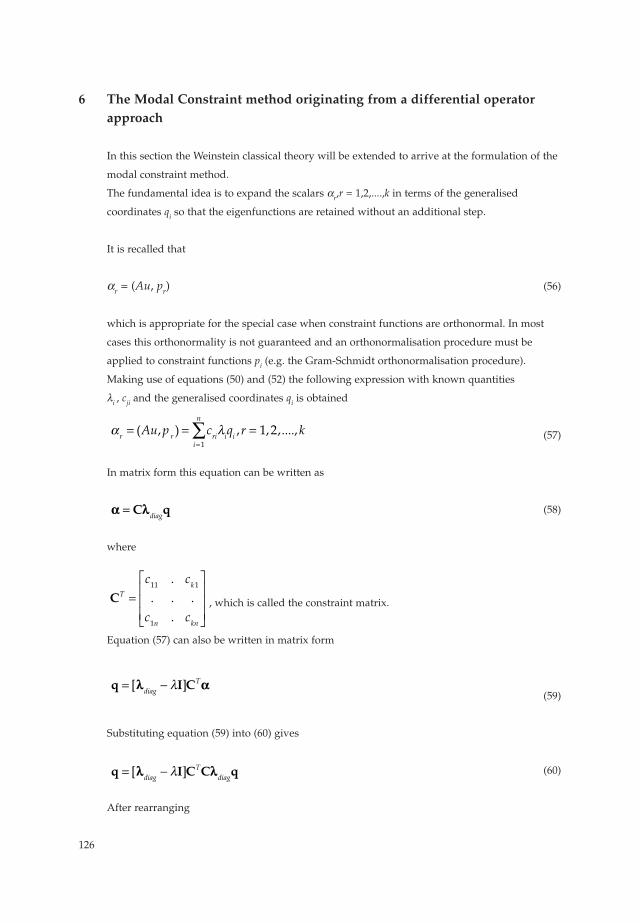
6 The Modal Constraint method originating from a differential operator
approach
In this section the Weinstein classical theory will be extended to arrive at the formulation of the
modal constraint method.
The fundamental idea is to expand the scalars αr,r = 1,2,....,k in terms of the generalised
coordinates qiso that the eigenfunctions are retained without an additional step.
It is recalled that
αr
= (Au, pr) (56)
which is appropriate for the special case when constraint functions are orthonormal. In most
cases this orthonormality is not guaranteed and an orthonormalisation procedure must be
applied to constraint functions pi(e.g. the Gram-Schmidt orthonormalisation procedure).
Making use of equations (50) and (52) the following expression with known quantities
λi , c
jiand the generalised coordinates q
iis obtained
(57)
In matrix form this equation can be written as
(58)
where
, which is called the constraint matrix.
Equation (57) can also be written in matrix form
(59)
Substituting equation (59) into (60) gives
(60)
After rearranging
q I C C q= −[ ]λλ λλdiagT
diagλ
q I C= −[ ]λλ ααdiagTλ
CTk
n kn
c c
c c=
⎡
⎣
⎢⎢⎢
⎤
⎦
⎥⎥⎥
11 1
1
.. . .
.
αα λλ= C qdiag
α λr r rii
n
i iAu p c q r k= = ==∑( , ) , , ,....,
1
1 2
126

(61)
Note that the left hand expression in the above matrix eigenvalue expression is asymmetric.
To arrive at symmetric matrices, equation (61) is again rearranged [6]
(62)
The above expression allows also persistent eigenvalues and multiple eigenvalues to be
evaluated with standard numerical eigenvalue methods.
Note that the constraint matrix CT needs to be orthonormalised row by row, which is due to the
requirement that the constraint functions pimust be orthonormal. This can be achieved by
applying the Gram-Schmidt orthonormalisation procedure. The short notation of equation (62)
takes the form of with two symmetric matrices. This eigenvalue expression
can be solved by standard numerical eigenvalue extraction procedures.
7 The modal constraint method in terms of energy: Lagrangian multipliers
Following the development given in [7] the energy functional for the constrained problem is
(63)
where L is the differential operator, and A is the domain of the problem.
The constraint energy that has to be subtracted from the energy of the unconstrained problem is
(64)
where α jare the Lagrangian multipliers.
A one-to-one correspondence between equations (57) and (64) leads to the conclusion that the
constraint forces to enforce the constraint are similar to
(65)
where (see equation (50))
(66)p c ur ri ii
n
==∑
1
αr rAu p= ( , )
W c qr r ri ii
n
==∑α
1
�uut
=∂∂
E Lu udA u u dA WA A
rr
k
= + −∫ ∫ ∑=
12
12 1
( ) ( , )ρ � �
[ ]A B q 0− =λ
[[ ] ] ;I C C q 0 q q− − = = −Tdiag diagλλλ λλ 1
[[ ] ]I C C I q 0− − =Tdiagλλ λ
127

Taking the first variation of equation (63) leads, after some elaboration, to the same eigenvalue
equation for the constrained problem as equation (62).
8 Practical example: four point supported square plate
In this section a specific example will be given where persistent eigenvalues will appear. It will
be shown that this will not pose any problems to extract these eigenvalues contrary to the
methods, which have similar expressions as equation (55).
The example consists of a four pointed supported square plate with three supports located at
the corners of the plate and one located at 0.15 of its diagonal length, see Figure 1.
Figure 1. Vibrating square plate: unconstrained problem and constrained problem
First let us introduce the formulation of the unconstrained problem, i.e. a completely free
vibrating square plate.
In [8] expressions for the unconstrained problem are given. It is also shown there how to
establish eigenvalues and eigenvectors based on beam functions of a completely free vibrating
rectangular plate. See Figure 2.
Note that also the three rigid body modes have to be added to the set of elastic mode shapes,
denoted by ψi ; i = 1,.., n .
Figure 2. Unconstrained problem: completely free vibrating plate: first three elastic mode shapes
The eigenvalue equation for the constrained problem, i.e. where point supports are added is
given below
Unconstrained problem Constrained problem
128

(67)
The elements of the orthonormalised constraint matrix CT are: cri
= ψi(ξ
r , η
r ) where there are
k constraint relations being the four point supports (ξ r , η
r ), r = 1,...,4 and i is the number of
modes.
The following results are obtained.
Table 1. Eigenvalues of the four point supported rectangular plate: .
First second third
Unconstrained problem 13.373 19.496 23.784
Constrained problem 8.596 15.646 19.496*)
*) persistent eigenvalue, i.e. common to both the unconstrained problem and the constrained
problem
This can be understood by examining the mode shapes of the constrained problem, see Figure 3.
Figure 3. Constrained problem: first three mode shapes: persistent eigenvalue.
The second mode shape of the unconstrained problem is equal to the third mode shape of the
constrained problem because all point supports are located at the nodal lines of the second
mode shape. The requirement of zero displacements is here already satisfied and therefore this
mode shape and its associated eigenvalue will be retained, i.e. persistent.
Using Weinstein’s determinant, Lagrangian multiplier method or receptance method will
present a problem because the persistent eigenvalue will make the dominator of expression (55)
zero and the value of the determinant infinitely large. When this is anticipated the considered
eigenvalues should be removed from the range of constrained eigenvalues. This is not always a
straightforward affair.
ω ρa D2 /
[[ ] ]I C C q 0− − =−Tdiagλλλ 1
129

9 Conclusions
The Lagrangian multiplier method and the receptance method have similar constrained
eigenvalue expressions to Weinstein’s determinant for intermediate problems of the first type.
These methods do not allow persistent eigenvalues to be present, i.e. those eigenvalues that are
common to both the unconstrained problem and the constrained problem.
To solve the resulting eigenvalue equations dedicated numerical solution procedures are
required such as the root finding procedures like the bi-section methods. However, persistent
eigenvalues stille pose a problem. One way of locating these eigenvalues is to plot the values of
the determinant of the eigenvalue equations. In cases where infinite values are obtained may
point in the direction of existing persistent eigenvalues. Even when this is successful multiple
eigenvalues cannot be found. These problems have not been sufficiently addressed in the
referenced literature. Once the eigevalues are established eigenvectors consisting of
Lagarangian multipliers can be obtained. Thereafter, the eigenvectors have to be transferred
into displacement eigenvectors to plot made shapes and/or to perform dynamic analyses.
In addition it should be noted that the Lagrangian multipliers represent the forces (or moments)
of constraint acting at the point to achieve zero displacements (or rotations).
The elements in the resulting eigenvalue equations can be regarded as influence coefficients. It
is well known that the Rayleigh-Ritz method provides upper bounds for the eigenvalues.
From the results obtained it can be concluded that the Lagrangian multiplier method also
referred in the literature component mode synthesis method or modal synthesis method
provides upper bounds for a fixed number of constraints and lower bounds for a fixed number
of component modes.
Comparing the Lagrangian multiplier method and the receptance method reveals that influence
coefficients have similar expressions as the receptances.
Weinstein’s method for intermediate problems of the first type allow the development of the
modal constraint method by realising that the Lagrangian multipliers can be expended into
known quantities, i.e. they are inner products of the unconstrained operator with constraint
functions, which in turn are related to the physical constraints.
The resulting constrained eigenvalue expression can be solved with standard numerical
eigenvalue routines. Also zero modal displacements (or rotations) do not pose a problem.
In the literature about Lagrangian multiplier methods and receptance methods no special
attention is paid to precautions needed to avoid an ill-conditioned state of the constraints
matrices. This can be diagnosed by applying the Gram-Schmidt orthonormalisation procedure,
130

which is a requirement for the modal constraint method. In other words, no remarks can be
found in the vast literature about the component mode synthesis method that the column
vectors in matrix need to be linearly independent, otherwise poor results may be obtained.
Also when constraining points are selected too close to each other the matrix may become ill
conditioned.
The results obtained by various authors show that increasing the number of constraints for a
fixed number of terms will result in lower bounds for the constrained eigenvalues whereas
increasing the number of terms for a fixed number of constraints will result in upper bounds as
is well-known for applying the classical Rayleigh-Ritz method. This hypothesis can be proved
to be true but in view of the available space it will be an issue for a separate paper.
It is pointed out that coupling unconstrained subsystems may also be treated by the methods
displayed. These problems merely require the differential modal displacements of the two
subsystems to be zero.
Finally, it is mentioned that also buckling of constrained linear mechanical systems can be
treated with the modal constraint method as buckling of structures can be seen as an
eigenvalue problem.
References
1. Courant-Hilbert, Methods of mathematical physics, Vol. 1, Interscience Publishers Inc.,NY,
1st Ed.
2. Gould, S.H., Variational methods of eigenvalue problems: An introduction to the
Weinstein method of intermediate problems, University of Toronto Press, 2nd Ed., 1966
3. Weinstein, A., Etude des spectres des equations aux derivees partielles de la theorie des
plaques elastiques, Memoires des sciences mathematique, fasc. 88, Gauthier-Villars, Paris
1937.
4. Budianski, Hu, The Lagrangian multiplier method for finding upper and lower limits to
critical stresses of clamped plates, NASA Special Publication, Report No. 848, 1946.
5. Bishop, R.E.D., Johnson, D.C., The mechanics of vibration, Cambridge University Press,
1960.
6. Dowell, E.H., Free vibration of linear structures with arbitrary support conditions, ASME
Journal of Applied Mechanics, 1971, Vol.38.
7. Kerstens, J.G.M., On the free vibrations of constrained linear mechanical systems, PhD
Thesis, University of Twente, The Netherlands, 1983.
8. Kerstens, J.G.M., Vibration of a rectangular plate at an arbitrary number of points, Journal
of Sound and Vibration, 1979, Vol.65.
131
9. Kerstens, J.G.M., Vibration of complex structures: the modal constraint method, Journal of
Sound and Vibration, 1981, Vol.76.
10. Kerstens, J.G.M., Vibration of constrained discrete systems: the modal constraint method,
Journal of Sound and Vibration, 1982, Vol.83.
11. Hurty, W.C., 1960, “Vibration of a Structural System by Component Mode Synthesis”,
J.Eng.Mech.Div., ASCE ,86, pp. 51-69.
12. Hurty, W.C., 1965, “Dynamic Analysis of Structural System Using Component
Modes”AIAA J., 3, pp. 678-685.
13. Craig, Jr.,R.R. and Brampton, M.C.C., 1968, “Coupling of Substructures for Dynamic
Analysis”, AIAA J., 6, pp. 131-1319.
14. Hou, S.N., 1969, “Review of Modal Synthesis Techniques and A New Approach”, The
Shock and Vibration Bulletin, 40, pp. 25-39.
15. Goldman, R.L., 1969, “Vibration Analysis by Dynamic Partioning”, AIAA J., 7, pp. 1152-
1154.
16. Dowell, E.H., 1972, “Free Vibration of an Arbitrary Structure in Terms of Component
Modes”, ASME J. Appl. Mech., 39, pp.727-732.
17. Rubin, S., 1975, “Improved Component-Mode Representation For Structural Dynamic
Analysis”, AIAA J., 13, pp. 995-1006.
18. Inamura, T., Suzuki H., and Sata T., 1994, “An Improved Method of Dynamic Coupling in
Structural Analysis and Its Application”, ASME J. Dyn. Syst. Meas. Control, 106, pp. 82-89.
19. Shankar, K., Keane, A.J., 1995,”Energy flow predictions in a structure of rigidly joined
beams using the receptance theory”, Journal of Sound and Vibration, 185, pp 867-890.
20. Moshref-Torbati, M., Keane, A.J., Elliot S.J., Brennan, M.J., Rogers, E. 2000, “The
integration of advanced active and passive structural vibration control”, Proceeding of
VETOMAC-I, India.
21. Wilkin, I.D., Soedel, W., 1976, “The receptance method applied to ring-stiffened cylindrical
shells: analysis of modal characteristics”, Journal of Sound and Vibration, 44, pp 563-576.
22. Azimi, S., Hamilton, J.F., Soedel, W., 1984, “The receptance method applied to the free
vibration of continuous rectangular plates”, Journal of Sound and Vibration, 93, pp 9-29.
23. Azimi, S., 1988, “Free vibration of circular plates with elastic edges support using the
receptance method”, Journal of Sound and Vibration, 120, pp 19-35.
132