a review and comparison of methods for detecting …d-scholarship.pitt.edu/7948/1/seo.pdf · a...
TRANSCRIPT

A Review and Comparison of Methods for Detecting Outliers in Univariate Data Sets
University of Pittsburgh
2006
Submitted to the Graduate Faculty of
Graduate School of Public Health in partial fulfillment
of the requirements for the degree of
Master of Science
by
Songwon Seo
BS, Kyunghee University, 2002

ii
UNIVERSITY OF PITTSBURGH
Graduate School of Public Health
This thesis was presented
by
Songwon Seo
It was defended on
April 26, 2006
and approved by:
Laura Cassidy, Ph D Assistant Professor
Department of Biostatistics Graduate School of Public Health
University of Pittsburgh
Ravi K. Sharma, Ph D Assistant Professor
Department of Behavioral and Community Health Sciences Graduate School of Public Health
University of Pittsburgh
Thesis Director: Gary M. Marsh, Ph D Professor
Department of Biostatistics Graduate School of Public Health
University of Pittsburgh

Gary M. Marsh, Ph D
Most real-world data sets contain outliers that have unusually large or small values when
compared with others in the data set. Outliers may cause a negative effect on data analyses, such
as ANOVA and regression, based on distribution assumptions, or may provide useful
information about data when we look into an unusual response to a given study. Thus, outlier
detection is an important part of data analysis in the above two cases. Several outlier labeling
methods have been developed. Some methods are sensitive to extreme values, like the SD
method, and others are resistant to extreme values, like Tukey’s method. Although these
methods are quite powerful with large normal data, it may be problematic to apply them to non-
normal data or small sample sizes without knowledge of their characteristics in these
circumstances. This is because each labeling method has different measures to detect outliers,
and expected outlier percentages change differently according to the sample size or distribution
type of the data.
Many kinds of data regarding public health are often skewed, usually to the right, and
lognormal distributions can often be applied to such skewed data, for instance, surgical
procedure times, blood pressure, and assessment of toxic compounds in environmental analysis.
This paper reviews and compares several common and less common outlier labeling methods
and presents information that shows how the percent of outliers changes in each method
according to the skewness and sample size of lognormal distributions through simulations and
application to real data sets. These results may help establish guidelines for the choice of outlier
detection methods in skewed data, which are often seen in the public health field.
iii
A Review and Comparison of Methods for Detecting Outliers in Univariate Data Sets
Songwon Seo, M.S.
University of Pittsburgh, 2006

iv
TABLE OF CONTENTS
1.0 INTRODUCTION ................................................................................................................ 1
1.1 BACKGROUND .......................................................................................................... 1
1.2 OUTLIER DETECTION METHOD ......................................................................... 3
2.0 STATEMENT OF PROBLEM ........................................................................................... 5
3.0 OUTLIER LABELING METHOD .................................................................................... 9
3.1 STANDARD DEVIATION (SD) METHOD ............................................................. 9
3.2 Z-SCORE.................................................................................................................... 10
3.3 THE MODIFIED Z-SCORE..................................................................................... 11
3.4 TUKEY’S METHOD (BOXPLOT) ......................................................................... 13
3.5 ADJUSTED BOXPLOT ............................................................................................ 14
3.6 MADE METHOD ....................................................................................................... 17
3.7 MEDIAN RULE......................................................................................................... 17
4.0 SIMULATION STUDY AND RESULTS FOR THE FIVE SELECTED LABELING
METHODS .................................................................................................................................. 19
5.0 APPLICATION .................................................................................................................. 32
6.0 RECOMMENDATIONS ................................................................................................... 36
7.0 DISCUSSION AND CONCLUSIONS.............................................................................. 38
APPENDIX A.............................................................................................................................. 40
THE EXPECTATION, STANDARD DEVIATION AND SKEWNESS OF A
LOGNORMAL DISTRIBUTION……………………………………………………………….40
APPENDIX B .............................................................................................................................. 42
MAXIMUM Z SCORE………………………………………………………………….42
APPENDIX C.............................................................................................................................. 44
CLASSICAL AND MEDCOUPLE (MC) SKEWNESS………………………………..44

v
APPENDIX D.............................................................................................................................. 47
BREAKDOWN POINT………………………………………………………………….47
APPENDIX E .............................................................................................................................. 48
PROGRAM CODE FOR OUTLIER LABELING METHODS………………………...48
BIBLIOGRAPHY....................................................................................................................... 51

vi
LIST OF TABLES
Table 1: Basic Statistic of a Simple Data Set ................................................................................. 2
Table 2: Basic Statistic After Changing 7 into 77 in the Simple Data Set ..................................... 2
Table 3: Computation and Masking Problem of the Z-Score ....................................................... 11
Table 4: Computation of Modified Z-Score and its Comparison with the Z-Score ..................... 12
Table 5: The Average Percentage of Left Outliers, Right Outliers and the Average Total Percent
of Outliers for the Lognormal Distributions with the Same Mean and Different Variances
(mean=0, variance=0.22, 0.42, 0.62, 0.82, 1.02) and the Standard Normal Distribution with
Different Sample Sizes. ................................................................................................................ 27
Table 6: Interval, Left, Right, and Total Number of Outliers According to the Five Outlier
Methods......................................................................................................................................... 34

vii
LIST OF FIGURES
Figure 1: Probability density function for a normal distribution according to the standard
deviation.......................................................................................................................................... 5
Figure 2: Theoretical Change of Outliers’ Percentage According to the Skewness of the
Lognormal Distributions in the SD Method and Tukey’s Method................................................ 7
Figure 3: Density Plot and Dotplot of the Lognormal Distribution (sample size=50) with Mean=1
and SD=1, and its Logarithm, Y=log(x). ........................................................................................ 8
Figure 4: Boxplot for the Example Data Set................................................................................. 13
Figure 5: Boxplot and Dotplot. (Note: No outlier shown in the boxplot).................................... 14
Figure 6: Change of theIintervals of Two Different Boxplot Methods ........................................ 16
Figure 7: Stnadard Normal Distribution and Lognormal Distributions........................................ 20
Figure 8: Change in the Outlier Percentages According to the Skewness of the Data................. 22
Figure 9: Change in the Total Percentages of Outliers According to the Sample Size ................ 25
Figure 10: Histogram and Basic Statistics of Case 1-Case 4........................................................ 32
Figure 11: Flowchart of Outlier Labeling Methods...................................................................... 37
Figure 12: Change of the Two Types of Skewness Coefficients According to the Sample Size
and Data Distribution. (Note: This results came from the previous simulation. All the values
are in Table 5 ) .............................................................................................................................. 46

1
1.0 INTRODUCTION
This chapter consists of two sections: the Background and Outlier Detection Method. In the
Background, basic ideas of an outlier are discussed such as definitions, features, and reasons to
detect outliers. In the Outlier Detection Method section, characteristics of the two kinds of
outlier detection methods are described briefly: formal and informal tests.
1.1 BACKGROUND
Observed variables often contain outliers that have unusually large or small values when
compared with others in a data set. Some data sets may come from homogeneous groups; others
from heterogeneous groups that have different characteristics regarding a specific variable, such
as height data not stratified by gender. Outliers can be caused by incorrect measurements,
including data entry errors, or by coming from a different population than the rest of the data. If
the measurement is correct, it represents a rare event. Two aspects of an outlier can be
considered.
The first aspect to note is that outliers cause a negative effect on data analysis. Osbome
and Overbay (2004) briefly categorized the deleterious effects of outliers on statistical analyses: 1) Outliers generally serve to increase error variance and reduce the power of statistical tests.
2) If non-randomly distributed, they can decrease normality (and in multivariate analyses, violate
assumptions of sphericity and multivariate normality), altering the odds of making both Type I and Type
II errors.
3) They can seriously bias or influence estimates that may be of substantive interest. The following example simply shows how one outlier can highly distort the mean,
variance, and 95% confidence interval for the mean. Let’s suppose there is a simple data set
composed of data points 1, 2, 3, 4, 5, 6, 7 and its basic statistics are as shown in Table 1. Now,

2
let’s replace data point 7 with 77. As shown in Table 2, the mean and variance of the data are
much larger than that of the original data set due to one unusual data value, 77. The 95%
confidence interval for the mean is also much broader because of the large variance. It may
cause potential problems when data analysis that is sensitive to a mean or variance is conducted.
Table 1: Basic Statistic of a Simple Data Set
Mean Median Variance 95 % Confidence Interval for the mean
4 4 4.67 [2.00 to 6.00]
Table 2: Basic Statistic After Changing 7 into 77 in the Simple Data Set
Mean Median Variance 95 % Confidence Interval for the mean
14 4 774.67 [-11.74 to 39.74]
The second aspect of outliers is that they can provide useful information about data when
we look into an unusual response to a given study. They could be the extreme values sitting
apart from the majority of the data regardless of distribution assumptions. The following two
cases are good examples of outlier analysis in terms of the second aspect of an outlier: 1) to
identify medical practitioners who under- or over-utilize specific procedures or medical
equipment, such as an x-ray instrument; 2) to identify Primary Care Physicians (PCPs) with
inordinately high Member Dissatisfaction Rates (MDRs) (MDRs = the number of member
complaints / PCP practice size) compared to other PCPs.23
In summary, there are two reasons for detecting outliers. The first reason is to find
outliers which influence assumptions of a statistical test, for example, outliers violating the
normal distribution assumption in an ANOVA test, and deal with them properly in order to
improve statistical analysis. This could be considered as a preliminary step for data analysis.
The second reason is to use the outliers themselves for the purpose of obtaining certain critical
information about the data as was shown in the above examples.

3
1.2 OUTLIER DETECTION METHOD
There are two kinds of outlier detection methods: formal tests and informal tests. Formal and
informal tests are usually called tests of discordancy and outlier labeling methods, respectively.
Most formal tests need test statistics for hypothesis testing. They are usually based on
assuming some well-behaving distribution, and test if the target extreme value is an outlier of the
distribution, i.e., weather or not it deviates from the assumed distribution. Some tests are for a
single outlier and others for multiple outliers. Selection of these tests mainly depends on
numbers and type of target outliers, and type of data distribution.1 Many various tests according
to the choice of distributions are discussed in Barnett and Lewis (1994) and Iglewicz and
Hoaglin (1993). Iglewicz and Hoaglin (1993) reviewed and compared five selected formal tests
which are applicable to the normal distribution, such as the Generalized ESD, Kurtosis statistics,
Shapiro-Wilk, the Boxplot rule, and the Dixon test, through simulations.
Even though formal tests are quite powerful under well-behaving statistical assumptions
such as a distribution assumption, most distributions of real-world data may be unknown or may
not follow specific distributions such as the normal, gamma, or exponential. Another limitation
is that they are susceptible to masking or swamping problems. Acuna and Rodriguez (2004)
define these problems as follows: Masking effect: It is said that one outlier masks a second outlier if the second outlier can be considered as
an outlier only by itself, but not in the presence of the first outlier. Thus, after the deletion of the first
outlier the second instance is emerged as an outlier.
Swamping effect: It is said that one outlier swamps a second observation if the latter can be considered as
an outlier only under the presence of the first one. In other words, after the deletion of the first outlier the
second observation becomes a non-outlying observation.
Many studies regarding these problems have been conducted by Barnett and Lewis (1994),
Iglewicz and Hoaglin (1993), Davies and Gather (1993), and Bendre and Kale (1987).
On the other hand, most outlier labeling methods, informal tests, generate an interval or
criterion for outlier detection instead of hypothesis testing, and any observations beyond the
interval or criterion is considered as an outlier. Various location and scale parameters are mostly
employed in each labeling method to define a reasonable interval or criterion for outlier detection.
There are two reasons for using an outlier labeling method. One is to find possible outliers as a
screening device before conducting a formal test. The other is to find the extreme values away

4
from the majority of the data regardless of the distribution. While the formal tests usually
require test statistics based on the distribution assumptions and a hypothesis to determine if the
target extreme value is a true outlier of the distribution, most outlier labeling methods present the
interval using the location and scale parameters of the data. Although the labeling method is
usually simple to use, some observations outside the interval may turn out to be falsely identified
outliers after a formal test when the outliers are defined as only observations that deviate from
the assuming distribution. However, if the purpose of the outlier detection is not a preliminary
step to find the extreme values violating the distribution assumptions of the main statistical
analyses such as the t-test, ANOVA, and regression, but mainly to find the extreme values away
from the majority of the data regardless of the distribution, the outlier labeling methods may be
applicable. In addition, for a large data set that is statistically problematic, e.g., when it is
difficult to identify the distribution of the data or transform it into a proper distribution such as
the normal distribution, labeling methods can be used to detect outliers.
This paper focuses on outlier labeling methods. Chapter 2 presents the possible problems
when labeling methods are applied to skewed data. In Chapter 3, seven outlier labeling methods
are outlined. In Chapter 4, the average percentages of outliers in the standard normal and log
normal distributions with the same mean and different variances is computed to compare the
outlier percentage of the selected five outlier labeling methods according to the degree of the
skewness and different sample sizes. In Chapter 5, the five selected methods are applied to real
data sets.

5
2.0 STATEMENT OF PROBLEM
Outlier-labeling methods such as the Standard Deviation (SD) and the boxplot are commonly
used and are easy to use. These methods are quite reasonable when the data distribution is
symmetric and mound-shaped such as the normal distribution. Figure 1 shows that about 68%,
95%, and 99.7% of the data from a normal distribution are within 1, 2, and 3 standard deviations
of the mean, respectively. If data follows a normal distribution, this helps to estimate the
likelihood of having extreme values in the data3, so that the observation two or three standard
deviations away from the mean may be considered as an outlier in the data.
Figure 1: Probability density function for a normal distribution according to the standard deviation.
The boxplot which was developed by Tukey (1977) is another very helpful method since
it makes no distributional assumptions nor does it depend on a mean or standard deviation.19
The lower quartile (q1) is the 25th percentile, and the upper quartile (q3) is the 75th percentile of
the data. The inter-quartile range (IQR) is defined as the interval between q1 and q3.

6
Tukey (1997) defined q1-(1.5*iqr) and q3+(1.5*iqr) as “inner fences”, q1-(3*iqr) and
q3+(3*iqr) as “outer fences”, the observations between an inner fence and its nearby outer fence
as “outside”, and anything beyond outer fences as “far out”.31 High (2000) renamed the
“outside” potential outliers and the “far out” problematic outliers.19 The “outside” and “far out”
observations can also be called possible outliers and probable outliers, respectively. This method
is quite effective, especially when working with large continuous data sets that are not highly
skewed.19
Although Tukey’s method is quite effective when working with large data sets that are
fairly normally distributed, many distributions of real-world data do not follow a normal
distribution. They are often highly skewed, usually to the right, and in such cases the
distributions are frequently closer to a lognormal distribution than a normal one.21 The
lognormal distribution can often be applied to such data in a variety of forms, for instance,
personal income, blood pressure, and assessment of toxic compounds in environmental analysis.
In order to illustrate how the theoretical percentage of outliers changes according to the skewness
of the data in the SD method (Mean ± 2 SD, Mean ± 3 SD) and Tukey’s method, lognormal
distributions with the same mean (0) but different standard deviations (0.2, 0.4, 0.6, 0.8, 1.0, 1.2)
are used for the data sets with different degrees of skewness, and the standard normal distribution
is used for the data set whose skewness is zero. The computation of the mean, standard
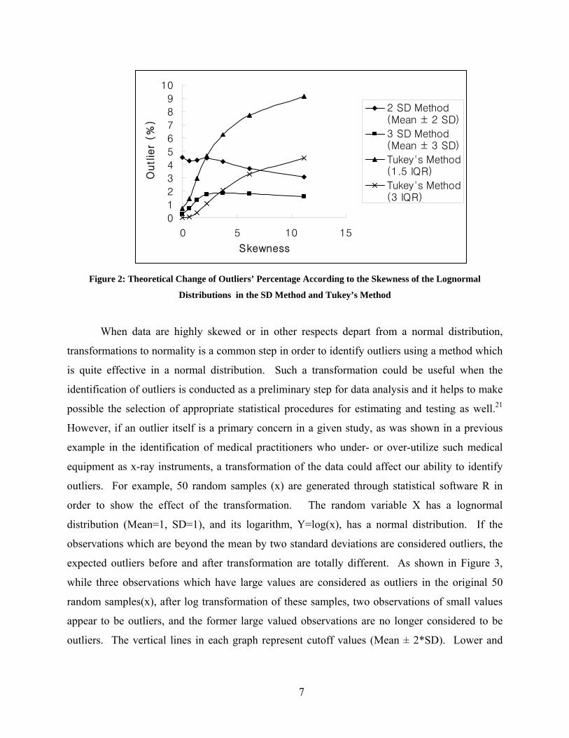
deviation, and skewness in a lognormal distribution is in Appendix A. According to Figure 2,
the two methods show a different pattern, e.g., the outlier percentage of Tukey’s method
increases, unlike the SD method. It shows that the results of outlier detection may change
depending on the outlier detection methods or the distribution of the data.
7
0
12
345
67
89
10
0 5 10 15
Skewness
Outlie
r (%
)
2 SD Method(Mean ± 2 SD)
3 SD Method(Mean ± 3 SD)
Tukey's Method(1.5 IQR)
Tukey's Method(3 IQR)
Figure 2: Theoretical Change of Outliers’ Percentage According to the Skewness of the Lognormal
Distributions in the SD Method and Tukey’s Method
When data are highly skewed or in other respects depart from a normal distribution,
transformations to normality is a common step in order to identify outliers using a method which
is quite effective in a normal distribution. Such a transformation could be useful when the
identification of outliers is conducted as a preliminary step for data analysis and it helps to make
possible the selection of appropriate statistical procedures for estimating and testing as well.21
However, if an outlier itself is a primary concern in a given study, as was shown in a previous
example in the identification of medical practitioners who under- or over-utilize such medical
equipment as x-ray instruments, a transformation of the data could affect our ability to identify
outliers. For example, 50 random samples (x) are generated through statistical software R in
order to show the effect of the transformation. The random variable X has a lognormal
distribution (Mean=1, SD=1), and its logarithm, Y=log(x), has a normal distribution. If the
observations which are beyond the mean by two standard deviations are considered outliers, the
expected outliers before and after transformation are totally different. As shown in Figure 3,
while three observations which have large values are considered as outliers in the original 50
random samples(x), after log transformation of these samples, two observations of small values
appear to be outliers, and the former large valued observations are no longer considered to be
outliers. The vertical lines in each graph represent cutoff values (Mean ± 2*SD). Lower and
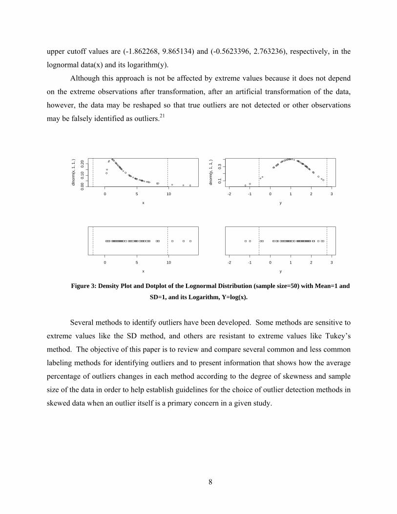
8
upper cutoff values are (-1.862268, 9.865134) and (-0.5623396, 2.763236), respectively, in the
lognormal data(x) and its logarithm(y).
Although this approach is not be affected by extreme values because it does not depend
on the extreme observations after transformation, after an artificial transformation of the data,
however, the data may be reshaped so that true outliers are not detected or other observations
may be falsely identified as outliers.21
0 5 10
0.00
0.10
0.20
x
dlno
rm(x
, 1, 1
, )
0 5 10
x
-2 -1 0 1 2 3
0.1
0.3
y
dnor
m(y
, 1, 1
, )
-2 -1 0 1 2 3
y Figure 3: Density Plot and Dotplot of the Lognormal Distribution (sample size=50) with Mean=1 and
SD=1, and its Logarithm, Y=log(x).
Several methods to identify outliers have been developed. Some methods are sensitive to
extreme values like the SD method, and others are resistant to extreme values like Tukey’s
method. The objective of this paper is to review and compare several common and less common
labeling methods for identifying outliers and to present information that shows how the average
percentage of outliers changes in each method according to the degree of skewness and sample
size of the data in order to help establish guidelines for the choice of outlier detection methods in
skewed data when an outlier itself is a primary concern in a given study.

9
3.0 OUTLIER LABELING METHOD
This chapter reviews seven outlier labeling methods and gives examples of simple numerical
computations for each test.
3.1 STANDARD DEVIATION (SD) METHOD
The simple classical approach to screen outliers is to use the SD (Standard Deviation) method. It
is defined as
2 SD Method: x ± 2 SD
3 SD Method: x ± 3 SD, where the mean is the sample mean and SD is the sample
standard deviation.
The observations outside these intervals may be considered as outliers. According to the
Chebyshev inequality, if a random variable X with mean μ and variance σ2 exists, then for any k
> 0,
1 ] |[| 2kkXP ≤≥− σμ
0 , 1 - 1 ] |[| 2 >≥<− kk
kXP σμ
the inequality [1-(1/k)2] enables us to determine what proportion of our data will be within k
standard deviations of the mean3. For example, at least 75%, 89%, and 94% of the data are
within 2, 3, and 4 standard deviations of the mean, respectively. These results may help us
determine the likelihood of having extreme values in the data3. Although Chebychev's therom is
true for any data from any distribution, it is limited in that it only gives the smallest proportion of
observations within k standard deviations of the mean22. In the case of when the distribution of a

10
random variable is known, a more exact proportion of observations centering around the mean
can be computed. For instance, if certain data follow a normal distribution, approximately 68%,
95%, and 99.7% of the data are within 1, 2, and 3 standard deviations of the mean, respectively;
thus, the observations beyond two or three SD above and below the mean of the observations
may be considered as outliers in the data.
The example data set, X, for a simple example of this method is as follows:
3.2, 3.4, 3.7, 3.7, 3.8, 3.9, 4, 4, 4.1, 4.2, 4.7, 4.8, 14, 15.
For the data set, x = 5.46, SD=3.86, and the intervals of the 2 SD and 3 SD methods are (-2.25,
13.18) and (-6.11, 17.04), respectively. Thus, 14 and 15 are beyond the interval of the 2 SD
method and there are no outliers in the 3 SD method.
3.2 Z-SCORE
Another method that can be used to screen data for outliers is the Z-Score, using the mean and
standard deviation.
sdxx
Z ii
−= , where Xi ~ N (µ, σ2), and sd is the standard deviation of data.
The basic idea of this rule is that if X follows a normal distribution, N (µ, σ2), then Z
follows a standard normal distribution, N (0, 1), and Z-scores that exceed 3 in absolute value are
generally considered as outliers. This method is simple and it is the same formula as the 3 SD
method when the criterion of an outlier is an absolute value of a Z-score of at least 3. It presents
a reasonable criterion for identification of the outlier when data follow the normal distribution.
According to Shiffler (1988), a possible maximum Z-score is dependent on sample size, and it is
computed as nn /)1( − . The proof is given in Appendix B. Since no z-score exceeds 3 in a
sample size less than or equal to 10, the z-score method is not very good for outlier labeling,
particularly in small data sets21. Another limitation of this rule is that the standard deviation can
be inflated by a few or even a single observation having an extreme value. Thus it can cause a
masking problem, i.e., the less extreme outliers go undetected because of the most extreme
outlier(s), and vice versa. When masking occurs, the outliers may be neighbors. Table 3 shows
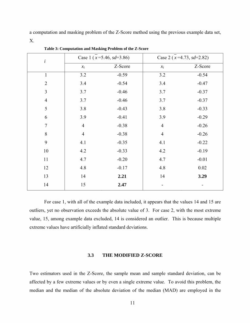
11
a computation and masking problem of the Z-Score method using the previous example data set,
X. Table 3: Computation and Masking Problem of the Z-Score
Case 1 ( x =5.46, sd=3.86) Case 2 ( x =4.73, sd=2.82) i
xi Z-Score xi Z-Score
1
2
3
4
5
6
7
8
9
10
11
12
13
14
3.2
3.4
3.7
3.7
3.8
3.9
4
4
4.1
4.2
4.7
4.8
14
15
-0.59
-0.54
-0.46
-0.46
-0.43
-0.41
-0.38
-0.38
-0.35
-0.33
-0.20
-0.17
2.21
2.47
3.2
3.4
3.7
3.7
3.8
3.9
4
4
4.1
4.2
4.7
4.8
14
-
-0.54
-0.47
-0.37
-0.37
-0.33
-0.29
-0.26
-0.26
-0.22
-0.19
-0.01
0.02
3.29
-
For case 1, with all of the example data included, it appears that the values 14 and 15 are
outliers, yet no observation exceeds the absolute value of 3. For case 2, with the most extreme
value, 15, among example data excluded, 14 is considered an outlier. This is because multiple
extreme values have artificially inflated standard deviations.
3.3 THE MODIFIED Z-SCORE
Two estimators used in the Z-Score, the sample mean and sample standard deviation, can be
affected by a few extreme values or by even a single extreme value. To avoid this problem, the
median and the median of the absolute deviation of the median (MAD) are employed in the

12
modified Z-Score instead of the mean and standard deviation of the sample, respectively
(Iglewicz and Hoaglin, 1993).
|}~{| xxmedianMAD i −= , where x~ is the sample median.
The modified Z-Score ( iM ) is computed as
MADxxM i
i)~(6745.0 −
= , where E( MAD )=0.675 σ for large normal data.
Iglewicz and Hoaglin (1993) suggested that observations are labeled outliers
when| iM |>3.5 through the simulation based on pseudo-normal observations for sample sizes of
10, 20, and 40.21 The iM score is effective for normal data in the same way as the Z-score.
Table 4: Computation of Modified Z-Score and its Comparison with the Z-Score
i xi Z-Score modified Z-Score
1
2
3
4
5
6
7
8
9
10
11
12
13
14
3.2
3.4
3.7
3.7
3.8
3.9
4
4
4.1
4.2
4.7
4.8
14
15
-0.59
-0.54
-0.46
-0.46
-0.43
-0.41
-0.38
-0.38
-0.35
-0.33
-0.20
-0.17
2.21
2.47
-1.80
-1.35
-0.67
-0.67
-0.45
-0.22
0
0
0.22
0.45
1.57
1.80
22.48
24.73
Table 4 shows the computation of the modified Z-Score and its comparison with the Z-
Score of the previous example data set. While no observation is detected as an outlier in the Z-
Score, two extreme values, 14 and 15, are detected as outliers at the same time in the modified Z-
Score since this method is less susceptible to the extreme values.
13
3.4 TUKEY’S METHOD (BOXPLOT)
Tukey’s (1977) method, constructing a boxplot, is a well-known simple graphical tool to display
information about continuous univariate data, such as the median, lower quartile, upper quartile,
lower extreme, and upper extreme of a data set. It is less sensitive to extreme values of the data
than the previous methods using the sample mean and standard variance because it uses quartiles
which are resistant to extreme values. The rules of the method are as follows:
1. The IQR (Inter Quartile Range) is the distance between the lower (Q1) and upper (Q3)
quartiles.
2. Inner fences are located at a distance 1.5 IQR below Q1 and above Q3 [Q1-1.5 IQR,
Q3+1.5IQR].
3. Outer fences are located at a distance 3 IQR below Q1 and above Q3 [Q1-3 IQR, Q3+3 IQR].
4. A value between the inner and outer fences is a possible outlier. An extreme value beyond the
outer fences is a probable outlier. There is no statistical basis for the reason that Tukey uses 1.5
and 3 regarding the IQR to make inner and outer fences.
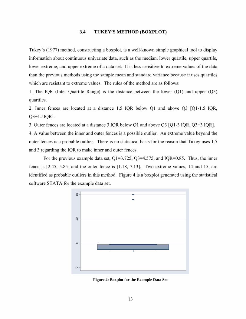
For the previous example data set, Q1=3.725, Q3=4.575, and IQR=0.85. Thus, the inner
fence is [2.45, 5.85] and the outer fence is [1.18, 7.13]. Two extreme values, 14 and 15, are
identified as probable outliers in this method. Figure 4 is a boxplot generated using the statistical
software STATA for the example data set.
05
1015
Figure 4: Boxplot for the Example Data Set
14
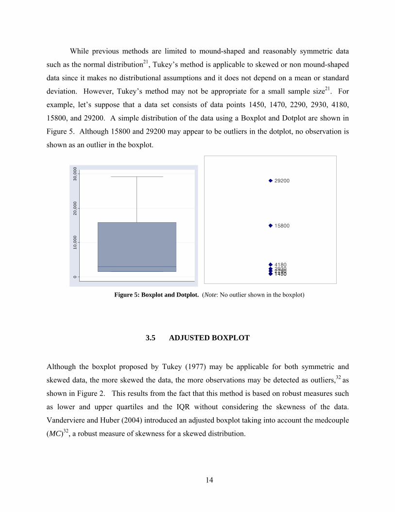
While previous methods are limited to mound-shaped and reasonably symmetric data
such as the normal distribution21, Tukey’s method is applicable to skewed or non mound-shaped
data since it makes no distributional assumptions and it does not depend on a mean or standard
deviation. However, Tukey’s method may not be appropriate for a small sample size21. For
example, let’s suppose that a data set consists of data points 1450, 1470, 2290, 2930, 4180,
15800, and 29200. A simple distribution of the data using a Boxplot and Dotplot are shown in
Figure 5. Although 15800 and 29200 may appear to be outliers in the dotplot, no observation is
shown as an outlier in the boxplot.
010
,000
20,0
0030
,000
14501470229029304180
15800
29200
Figure 5: Boxplot and Dotplot. (Note: No outlier shown in the boxplot)
3.5 ADJUSTED BOXPLOT
Although the boxplot proposed by Tukey (1977) may be applicable for both symmetric and
skewed data, the more skewed the data, the more observations may be detected as outliers,32 as
shown in Figure 2. This results from the fact that this method is based on robust measures such
as lower and upper quartiles and the IQR without considering the skewness of the data.
Vanderviere and Huber (2004) introduced an adjusted boxplot taking into account the medcouple
(MC)32, a robust measure of skewness for a skewed distribution.

15
When Xn={ nxxx ,...,, 21 } is a data set independently sampled from a continuous
univariate distribution and it is sorted such as nxxx ≤≤≤ ...21 , the MC of the data is defined as
ij
ikkjn xx
xmedmedxmedxxMC
−
−−−=
)()(),...,( 1 ,where kmed is the median of Xn, and i
and j have to satisfy ix ≤ kmed ≤ jx , and ix ≠ jx . The interval of the adjusted boxplot is as
follows (G. Bray et al. (2005)):
[L, U] = [Q1-1.5 * exp (-3.5MC) * IQR, Q3+1.5 * exp (4MC) * IQR] if MC ≥ 0
= [Q1-1.5 * exp (-4MC) * IQR, Q3+1.5 * exp (3.5MC) * IQR] if MC ≤ 0,
where L is the lower fence, and U is the upper fence of the interval. The observations which fall
outside the interval are considered outliers.
The value of the MC ranges between -1 and 1. If MC=0, the data is symmetric and the
adjusted boxplot becomes Tukey’s box plot. If MC>0, the data has a right skewed distribution,
whereas if MC<0, the data has a left skewed distribution.32 A simple example for computation of
MC and a brief comparison of classical and MC skewness are in Appendix C.
For the previous example data set, Q1=3.725, Q3=4.575, IQR=0.85, and MC=0.43. Thus,
the interval of the adjusted boxplot is [3.44, 11.62]. Two extreme values, 14 and 15, and the two
smallest values, 3.2 and 3.4, are identified as outliers in this method. Figure 6 shows the change
of the intervals of two boxplot methods, Tukey’s method and the adjusted boxplot, for the
example data set. The vertical dotted lines are the lower and upper bound of the interval of each
method. Although the example data set is artificial and is not large enough to explain their
difference, we can see a general trend that the interval of the adjusted boxplot, especially the
upper fence, moves to the side of the skewed tail, compared to Tukey’s method.

16
5 10 15
Inner fences of Tukey Method (Q1-1.5*IQR, Q3+1.5*IQR)
5 10 15
Outer fences of Tukey Method (Q1-3*IQR, Q3+3IQR)
5 10 15
Single fence of adjusted box plot (Q1-1.5 * exp (-3.5MC) * IQR, Q3+1.5 * exp (4MC) * IQR)
Figure 6: Change of theIintervals of Two Different Boxplot Methods
(Tukey’s Method vs. the Adjusted Boxplot)
Vanderviere and Huber (2004) computed the average percentage of outliers beyond the
lower and upper fence of two types of boxplots, the adjusted Boxplot and Tukey’s Boxplot, for
several distributions and different sample sizes. In the simulation, less observations, especially
in the right tail, are classified as outliers compared to Tukey’s method when the data are skewed
to the right.32 In the case of a mildly right-skewed distribution, the lower fence of the interval
may move to the right and more observations in the left side will be classified as outliers
compared to Tukey’s method. This difference mainly comes from a decrease in the lower fence
and an increase in the upper fence from Q1 and Q3, repectively.32
17
3.6 MADE METHOD
The MADe method, using the median and the Median Absolute Deviation (MAD), is one of the
basic robust methods which are largely unaffected by the presence of extreme values of the data
set.11 This approach is similar to the SD method. However, the median and MADe are
employed in this method instead of the mean and standard deviation. The MADe method is
defined as follows;
2 MADe Method: Median ± 2 MADe
3 MADe Method: Median ± 3 MADe,
where MADe=1.483×MAD for large normal data.
MAD is an estimator of the spread in a data, similar to the standard deviation11, but has
an approximately 50% breakdown point like the median21. The notion of breakdown point is
delineated in Appendix D.
MAD= median (|xi – median(x)| i=1,2,…,n)
When the MAD value is scaled by a factor of 1.483, it is similar to the standard deviation
in a normal distribution. This scaled MAD value is the MADe.
For the example data set, the median=4, MAD=0.3, and MADe=0.44. Thus, the intervals
of the 2 MADe and 3 MADe methods are [3.11, 4.89] and [2.67, 5.33], respectively.
Since this approach uses two robust estimators having a high breakdown point, i.e., it is
not unduly affected by extreme values even though a few observations make the distribution of
the data skewed, the interval is seldom inflated, unlike the SD method.
3.7 MEDIAN RULE
The median is a robust estimator of location having an approximately 50% breakdown point. It
is the value that falls exactly in the center of the data when the data are arranged in order.
18
That is, if x1, x2, …, xn is a random sample sorted by order of magnitude, then the median
is defined as:
Median, x~ = xm when n is odd
x~ = (xm+xm+1)/2 when n is even, where m=round up (n/2)
For a skewed distribution like income data, the median is often used in describing the
average of the data. The median and mean have the same value in a symmetrical distribution.
Carling (1998) introduces the median rule for identification of outliers through studying
the relationship between target outlier percentage and Generalized Lambda Distributions (GLDs).
GLDs with different parameters are used for various moderately skewed distributions12. The
median substitutes for the quartiles of Tukey’s method, and a different scale of the IQR is
employed in this method. It is more resistant and its target outlier percentage is less affected by
sample size than Tukey’s method in the non-Gaussian case12. The scale of IQR can be adjusted
depending on which target outlier percentage and GLD are selected. In my paper, 2.3 is chosen
as the scale of IQR; when the scale is applied to normal distribution, the outlier percentage turns
out to be between Tukey’s method of 1.5 IQR and that of 3 IQR, i.e., 0.2 %.
It is defined as:
[C1, C2]=Q2± 2.3 IQR, where Q2 is the sample median.
For the example data set, Q2=4, and IQR=0.85. Thus, the interval of this method is [2.05,
5.96].

19
4.0 SIMULATION STUDY AND RESULTS FOR THE FIVE SELECTED LABELING
METHODS
Most intervals or criteria to identify possible outliers in outlier labeling methods are effective
under the normal distribution. For example, in the case of a well-known labeling method such as
the 2 SD and 3 SD methods and the Boxplot (1.5 IQR), the expected percentages of observations
outside the interval are 5%, 0.3%, and 0.7%, respectively, under large normal samples.
Although these methods are quite powerful with large normal data, it may be problematic to
apply them to non-normal data or small sample sizes without information about their
characteristics in these circumstances. This is because each labeling method has different
measures to detect outliers, and expected outlier percentages change differently according to the
sample size or distribution type of the data.
The purpose of this simulation is to present the expected percentage of the observations
outside of the interval of several labeling methods according to the sample size and the degree of
the skewness of the data using the lognormal distribution with the same mean and different
variances. Through this simulation, we can know not only the possible outlier percentage of
several labeling methods but also which method is more robust according to the above two
factors, skewness and sample size. The simulation proceeds as follows:
Five labeling methods are selected: the SD Method, the MADe Method, Tukey’s Method
(Boxplot), Adjusted Boxplot, and the Median Rule. The Z-Score and modified Z-Score are not
considered because their criteria to define an outlier are based on the normal distribution.
Average outlier percentages of five labeling methods in the standard normal (0,1) and
lognormal distributions with the same mean and different variances (mean=0, variance=0.22, 0.42,
0.62, 0.82, 12) are computed. For each distribution, 1000 replications of sample sizes 20 and 50,
300 replications of the sample size 100, and 100 replications of the sample sizes 300 and 500 are
considered. To illustrate the shape of each distribution, i.e., the degree of skewness of the data,
20
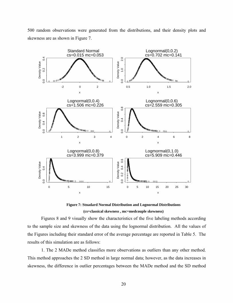
500 random observations were generated from the distributions, and their density plots and
skewness are as shown in Figure 7.
x
Den
sity
Val
ue
-2 0 2
0.0
0.2
0.4
Standard Normal cs=0.015 mc=0.053
x
Den
sity
Val
ue
0.5 1.0 1.5 2.0
0.0
1.0
2.0
Lognormal(0,0.2) cs=0.702 mc=0.141
x
Den
sity
Val
ue
1 2 3 4
0.0
0.4
0.8
Lognormal(0,0.4) cs=1.506 mc=0.226
x
Den
sity
Val
ue
0 2 4 6 8
0.0
0.4
0.8
Lognormal(0,0.6) cs=2.559 mc=0.305
x
Den
sity
Val
ue
0 5 10 15
0.0
0.4
Lognormal(0,0.8) cs=3.999 mc=0.379
x
Den
sity
Val
ue
0 5 10 15 20 25 30
0.0
0.2
0.4
0.6
Logmormal(0,1.0) cs=5.909 mc=0.446
Figure 7: Stnadard Normal Distribution and Lognormal Distributions
(cs=classical skewness , mc=medcouple skewness)
Figures 8 and 9 visually show the characteristics of the five labeling methods according
to the sample size and skewness of the data using the lognormal distribution. All the values of
the Figures including their standard error of the average percentage are reported in Table 5. The
results of this simulation are as follows:
1. The 2 MADe method classifies more observations as outliers than any other method.
This method approaches the 2 SD method in large normal data; however, as the data increases in
skewness, the difference in outlier percentages between the MADe method and the SD method

21
becomes larger since the location and scale measures such as the median and MADe become the
same as the mean and standard variance of the SD method when data follows a normal
distribution with a large sample size. The MADe, Tukey’s method, and the Median rule increase
in the total average percentages of outliers the more skewed the data, while the SD method and
adjusted boxplot seldom change over different sample sizes.
2. The Median rule classifies less observations than Tukey’s 1.5 IQR method and more
observations than Tukey’s 3 IQR method.
3. The decrease range of the total outlier percentage of the adjusted boxplot is larger than
other methods as the sample size increases.
4. Most methods except the adjusted boxplot show similar patterns in the average outlier
percentages on the left side of the distribution. They decrease in left outlier percentage rapidly,
especially in 2 MADe and 2 SD methods, the more skewed the data; however, the adjusted
boxplot decreases slowly in sample sizes over 300. Different patterns of the adjusted boxplot,
e.g., increase in left outlier percentage in small sample sizes, may be due to the following:
• The left fence of the interval may move to the right side because of the MC skewness
and a few observations may be distributed outside the left fence by chance.
• Although the number of the observations is small, the ratio in a small sample size could
large. This may affect an increase in the average of the percentage of outliers on the left of the
distribution.
• The adjusted boxplot may still detect observations on the left side of the distribution in
right skewed data, especially mildly skewed data; however, the average percentages are quiet
low.
5. The MADe, Tukey’s method, and the Median rule increase in the percentage of
outliers on the right side of the distribution as the skewness of the data increases while the SD
method and adjusted boxplot seldom change in each sample size (the SD method increases
slightly and plateaus). The right fence of the intervals of both methods, the SD method and
adjusted boxplot, move to the right side of the distribution as the skewness of the data increases.
Since the adjusted boxplot takes into account the skewness of the data, its right fence of the
interval moves more to the side of the skewed tail, here the right side of the distribution, as the
skewness increases. On the other hand, the interval of the SD method is just inflated because of
the extreme values.

22
Sample size 20
Sample size 50
Figure 8: Change in the Outlier Percentages According to the Skewness of the Data

23
Sample100
Sample size 300
Figure 8 (continued)

24
Sample size 500
Figure 8 (continued)

25
Figure 9: Change in the Total Percentages of Outliers According to the Sample Size
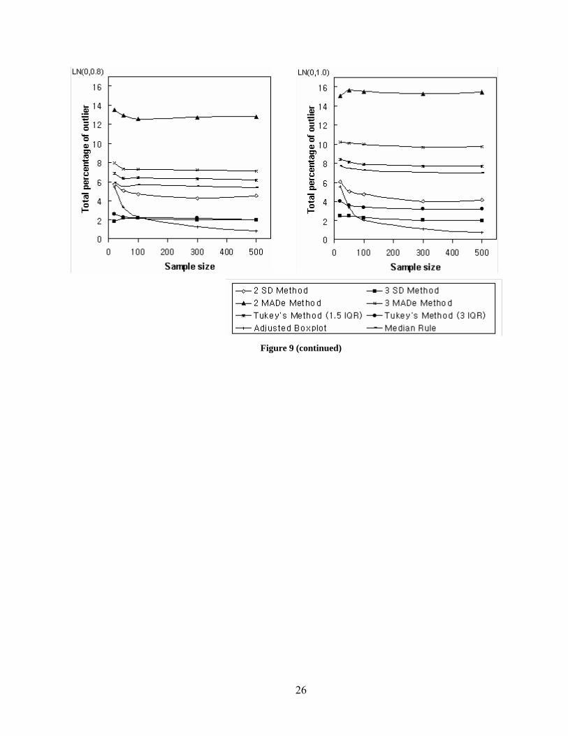
26
Figure 9 (continued)

27
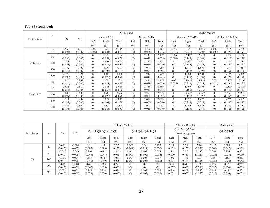
Table 5: The Average Percentage of Left Outliers, Right Outliers and the Average Total Percent of Outliers for the Lognormal Distributions with the
Same Mean and Different Variances (mean=0, variance=0.22, 0.42, 0.62, 0.82, 1.02) and the Standard Normal Distribution with Different Sample Sizes.
SD Method MADe Method Mean ± 2 SD Mean ± 3 SD Median ± 2 MADe Median ± 3 MADe
Distribution n
CS MC Left (%)
Right (%)
Total (%)
Left (%)
Right (%)
Total (%)
Left (%)
Right (%)
Total (%)
Left (%)
Right (%)
Total (%)
20 0.006 (0.015)
-0.004 (0.007)
1.865 (0.080)
1.87 (0.083)
3.735 (0.101)
0.03 (0.012)
0.025 (0.011)
0.055 (0.016)
3.35 (0.150)
3.53 (0.156)
6.88 (0.241)
0.685 (0.066)
0.77 (0.073)
1.455 (0.109)
50 -0.017 (0.010)
-0.009 (0.005)
2.176 (0.053)
2.09 (0.052)
4.266 (0.063)
0.086 (0.013)
0.076 (0.012)
0.162 (0.017)
2.948 (0.095)
2.676 (0.088)
5.624 (0.141)
0.366 (0.032)
0.296 (0.027)
0.662 (0.045)
100 -0.006 (0.013)
0.001 (0.006)
2.26 (0.066)
2.19 (0.060)
4.45 (0.079)
0.093 (0.017)
0.113 (0.020)
0.207 (0.026)
2.637 (0.115)
2.573 (0.109)
5.21 (0.184)
0.233 (0.032)
0.253 (0.036)
0.487 (0.055)
300 0.006 (0.015)
0.0004 (0.006)
2.267 (0.073)
2.307 (0.060)
4.573 (0.086)
0.117 (0.019)
0.14 (0.021)
0.257 (0.026)
2.347 (0.121)
2.31 (0.099)
4.657 (0.173)
0.167 (0.029)
0.18 (0.028)
0.347 (0.042)
SN
500 -0.008 (0.010)
0.004 (0.005)
2.266 (0.051)
2.17 (0.047)
4.436 (0.059)
0.13 (0.016)
0.138 (0.017)
0.268 (0.025)
2.2 (0.078)
2.17 (0.080)
4.37 (0.133)
0.146 (0.019)
0.148 (0.019)
0.294 (0.029)
20 0.436 (0.016)
0.084 (0.007)
0.555 (0.050)
3.195 (0.092)
3.75 (0.095)
0 (0)
0.2 (0.031)
0.2 (0.031)
1.615 (0.110)
5.67 (0.183)
7.285 (0.227)
0.195 (0.034)
1.765 (0.108)
1.96 (0.119)
50 0.527 (0.012)
0.086 (0.005)
0.71 (0.037)
3.434 (0.055)
4.144 (0.059)
0 (0)
0.508 (0.028)
0.508 (0.028)
1.16 (0.060)
5.092 (0.114)
6.252 (0.141)
0.03 (0.008)
1.334 (0.057)
1.364 (0.059)
100 0.574 (0.018)
0.079 (0.006)
0.723 (0.052)
3.57 (0.073)
4.293 (0.076)
0.003 (0.003)
0.623 (0.038)
0.627 (0.038)
0.93 (0.077)
4.96 (0.139)
5.89 (0.168)
0.017 (0.009)
1.113 (0.065)
1.13 (0.067)
300 0.604 (0.020)
0.093 (0.006)
0.676 (0.044)
3.49 (0.071)
4.167 (0.081)
0 (0)
0.657 (0.035)
0.657 (0.035)
0.737 (0.060)
4.947 (0.160)
5.683 (0.185)
0 (0)
1.09 (0.068)
1.09 (0.068)
LN (0, 0.2)
500 0.609 (0.015)
0.094 (0.004)
0.594 (0.035)
3.602 (0.064)
4.196 (0.065)
0 (0)
0.71 (0.029)
0.71 (0.029)
0.524 (0.040)
4.73 (0.116)
5.254 (0.132)
0 (0)
1.024 (0.051)
1.024 (0.051)
20 0.864 (0.020)
0.161 (0.007)
0.095 (0.022)
4.385 (0.090)
4.48 (0.090)
0 (0)
0.715 (0.055)
0.715 (0.055)
0.795 (0.091)
8.15 (0.197)
8.945 (0.225)
0.07 (0.030)
3.51 (0.141)
3.58 (0.144)
50 1.062 (0.017)
0.170 (0.005)
0.04 (0.009)
4.522 (0.055)
4.562 (0.054)
0 (0)
1.132 (0.037)
1.132 (0.037)
0.234 (0.025)
7.816 (0.127)
8.05 (0.133)
0.002 (0.002)
3.068 (0.084)
3.07 (0.085)
100 1.143 (0.027)
0.181 (0.007)
0.02 (0.008)
4.46 (0.073)
4.48 (0.073)
0 (0)
1.157 (0.044)
1.157 (0.044)
0.107 (0.023)
7.743 (0.168)
7.85 (0.173)
0 (0)
2.763 (0.110)
2.763 (0.110)
300 1.251 (0.033)
0.167 (0.006)
0.007 (0.005)
4.297 (0.065)
4.303 (0.066)
0 (0)
1.247 (0.046)
1.247 (0.046)
0.033 (0.014)
7.3 (0.158)
7.333 (0.163)
0 (0)
2.467 (0.094)
2.467 (0.094)
LN (0, 0.4)
500 1.303 (0.025)
0.170 (0.005)
0.002 (0.002)
4.244 (0.056)
4.246 (0.057)
0 (0)
1.296 (0.032)
1.296 (0.032)
0.014 (0.005)
7.518 (0.149)
7.532 (0.151)
0 (0)
2.684 (0.074)
2.684 (0.074)
20 1.212 (0.024)
0.219 (0.007)
0 (0)
5.035 (0.084)
5.035 (0.084)
0 (0)
1.3 (0.069)
1.3 (0.069)
0.24 (0.042)
9.965 (0.216)
10.205(0.224)
0.005 (0.005)
5.150 (0.164)
5.155 (0.165)
50 1.623 (0.024)
0.250 (0.005)
0 (0)
4.868 (0.056)
4.868 (0.056)
0 (0)
1.74 (0.038)
1.74 (0.038)
0.034 (0.011)
10.39 (0.140)
10.424(0.140)
0 (0)
5.008 (0.105)
5.008 (0.105)
100 1.774 (0.039)
0.251 (0.006)
0 (0)
4.793 (0.074)
4.793 (0.074)
0 (0)
1.777 (0.050)
1.777 (0.050)
0.01 (0.01)
10.047 (0.170)
10.057(0.171)
0 (0)
4.963 (0.133)
4.963 (0.133)
300 2.120 (0.063)
0.254 (0.007)
0 (0)
4.413 (0.086)
4.413 (0.086)
0 (0)
1.817 (0.051)
1.817 (0.051)
0 (0)
10.23 (0.178)
10.23 (0.178)
0 (0)
4.877 (0.146)
4.877 (0.146)
LN (0, 0.6)
500 2.199 (0.064)
0.255 (0.005)
0 (0)
4.368 (0.068)
4.368 (0.068)
0 (0)
1.68 (0.047)
1.68 (0.047)
0 (0)
10.124 (0.145)
10.124(0.145)
0 (0)
4.724 (0.106)
4.724 (0.106)
28
Table 5 (continued)
SD Method MADe Method Mean ± 2 SD Mean ± 3 SD Median ± 2 MADe Median ± 3 MADe
Distribution n
CS MC Left (%)
Right (%)
Total (%)
Left (%)
Right (%)
Total (%)
Left (%)
Right (%)
Total (%)
Left (%)
Right (%)
Total (%)
20 1.560 (0.024)
0.31 (0.007)
0.005 (0.005)
5.71 (0.081)
5.715 (0.081)
0 (0)
1.86 (0.076)
1.86 (0.076)
0.095 (0.031)
13.4 (0.218)
13.495(0.224)
0.005 (0.005)
7.915 (0.191)
7.92 (0.191)
50 2.126 (0.030)
0.315 (0.005)
0 (0)
5.05 (0.058)
5.05 (0.058)
0 (0)
2.132 (0.038)
2.132 (0.038)
0.006 (0.004)
12.932 (0.143)
12.938(0.144)
0 (0)
7.33 (0.120)
7.33 (0.120)
100 2.548 (0.058)
0.314 (0.007)
0 (0)
4.693 (0.084)
4.693 (0.084)
0 (0)
2.177 (0.049)
2.177 (0.049)
0 (0)
12.577 (0.183)
12.577(0.183)
0 (0)
7.283 (0.151)
7.283 (0.151)
300 3.179 (0.152)
0.327 (0.007)
0 (0)
4.25 (0.103)
4.25 (0.103)
0 (0)
1.967 (0.053)
1.967 (0.053)
0 (0)
12.75 (0.193)
12.75 (0.193)
0 (0)
7.217 (0.160)
7.217 (0.160)
LN (0, 0.8)
500 2.928 (0.096)
0.324 (0.005)
0 (0)
4.48 (0.076)
4.48 (0.076)
0 (0)
1.942 (0.041)
1.942 (0.041)
0 (0)
12.84 (0.132)
12.84 (0.132)
0 (0)
7.09 (0.120)
7.09 (0.120)
20 1.876 (0.026)
0.353 (0.007)
0 (0)
6.03 (0.078)
6.03 (0.078)
0 (0)
2.455 (0.079)
2.455 (0.079)
0.05 (0.025)
15.065 (0.217)
15.115(0.218)
0.02 (0.016)
10.175 (0.195)
10.195(0.195)
50 2.626 (0.034)
0.384 (0.005)
0 (0)
5.048 (0.060)
5.048 (0.060)
0 (0)
2.486 (0.037)
2.486 (0.037)
0 (0)
15.65 (0.152)
15.65 (0.152)
0 (0)
10.124 (0.133)
10.124(0.133)
100 3.086 (0.079)
0.400 (0.006)
0 (0)
4.76 (0.096)
4.76 (0.096)
0 (0)
2.273 (0.051)
2.273 (0.051)
0 (0)
15.527 (0.190)
15.527(0.190)
0 (0)
9.963 (0.165)
9.963 (0.165)
300 4.113 (0.183)
0.399 (0.007)
0 (0)
4.027 (0.108)
4.027 (0.108)
0 (0)
2.013 (0.060)
2.013 (0.060)
0 (0)
15.26 (0.211)
15.26 (0.211)
0 (0)
9.67 (0.187)
9.67 (0.187)
LN (0, 1.0)
500 4.052 (0.155)
0.394 (0.005)
0 (0)
4.15 (0.085)
4.15 (0.085)
0 (0)
1.992 (0.046)
1.992 (0.046)
0 (0)
15.43 (0.137)
15.43 (0.137)
0 (0)
9.732 (0.126)
9.732 (0.126)
Tukey’s Method Adjusted Boxplot Median Rule
Q1-1.5 IQR / Q3+1.5 IQR Q1-3 IQR / Q3+3 IQR Q1-1.5exp(-3.5mc)/
Q3+1.5exp(4mc) Q2 ±2.3 IQR
Distribution n CS MC Left (%)
Right (%)
Total (%)
Left (%)
Right (%)
Total (%)
Left (%)
Right (%)
Total (%)
Left (%)
Right (%)
Total (%)
20 0.006 (0.015)
-0.004 (0.007)
1.1 (0.083)
1.17 (0.089)
2.27 (0.137)
0.065 (0.019)
0.04 (0.014)
0.105 (0.026)
2.39 (0.135)
2.75 (0.153)
5.14 (0.178)
0.615 (0.061)
0.685 (0.067)
1.3 (0.102)
50 -0.017 (0.010)
-0.009 (0.005)
0.704 (0.043)
0.66 (0.041)
1.364 (0.065)
0.006 (0.003)
0.002 (0.002)
0.008 (0.004)
1.462 (0.090)
2.07 (0.110)
3.532 (0.121)
0.292 (0.028)
0.236 (0.024)
0.528 (0.039)
100 -0.006 (0.013)
0.001 (0.006)
0.537 (0.049)
0.51 (0.049)
1.047 (0.078)
0.003 (0.003)
0.003 (0.003)
0.007 (0.005)
1.05 (0.101)
1.18 (0.107)
2.23 (0.125)
0.18 (0.026)
0.183 (0.028)
0.363 (0.042)
300 0.006 (0.015)
0.0004 (0.006)
0.42 (0.045)
0.363 (0.038)
0.783 (0.061)
0 (0)
0 (0)
0 (0)
0.59 (0.077)
0.647 (0.093)
1.237 (0.098)
0.127 (0.025)
0.13 (0.024)
0.257 (0.035)
SN
500 -0.008 (0.010)
0.004 (0.005)
0.342 (0.029)
0.354 (0.030)
0.696 (0.047)
0 (0)
0.002 (0.002)
0.002 (0.002)
0.564 (0.071)
0.468 (0.057)
0.892 (1.172)
0.112 (0.016)
0.11 (0.016)
0.222 (0.023)

29
Table 5 (continued)
Tukey’s Method Adjusted Boxplot Median Rule
Q1-1.5 IQR / Q3+1.5 IQR Q1-3 IQR / Q3+3 IQR Q1-1.5exp(-3.5mc)/
Q3+1.5exp(4mc) Q2 ±2.3 IQR
Distribution n CS MC Left (%)
Right (%)
Total (%)
Left (%)
Right (%)
Total (%)
Left (%)
Right (%)
Total (%)
Left (%)
Right (%)
Total (%)
20 0.436 (0.016)
0.084 (0.007)
0.415 (0.052)
2.29 (0.113)
2.705 (0.137)
0 (0)
0.21 (0.033)
0.21 (0.033)
2.725 (0.146)
2.395 (0.143)
5.12 (0.177)
0.19 (0.035)
1.575 (0.098)
1.765 (0.111)
50 0.527 (0.012)
0.086 (0.005)
0.146 (0.020)
1.806 (0.067)
1.952 (0.075)
0 (0)
0.108 (0.015)
0.108 (0.015)
1.864 (0.103)
1.548 (0.091)
3.412 (0.118)
0.028 (0.008)
1.114 (0.052)
1.142 (0.054)
100 0.574 (0.018)
0.079 (0.006)
0.063 (0.012)
1.6 (0.076)
1.663 (0.078)
0 (0)
0.063 (0.015)
0.063 (0.015)
0.95 (0.101)
1.1 (0.103)
2.05 (0.125)
0.003 (0.003)
0.913 (0.055)
0.917 (0.055)
300 0.604 (0.020)
0.093 (0.006)
0.02 (0.009)
1.587 (0.086)
1.607 (0.086)
0 (0)
0.077 (0.016)
0.077 (0.016)
0.82 (0.103)
0.543 (0.068)
1.363 (0.097)
0 (0)
0.94 (0.064)
0.94 (0.064)
LN (0. 0.2)
500 0.609 (0.015)
0.094 (0.004)
0.012 (0.006)
1.512 (0.060)
1.524 (0.060)
0 (0)
0.036 (0.009)
0.036 (0.009)
0.472 (0.070)
0.356 (0.039)
0.828 (0.066)
0 (0)
0.838 (0.044)
0.838 (0.044)
20 0.864 (0.020)
0.161 (0.007)
0.145 (0.033)
3.805 (0.131)
3.95 (0.139)
0 (0)
0.755 (0.063)
0.755 (0.063)
2.785 (0.153)
2.16 (0.130)
4.945 (0.175)
0.025 (0.011)
2.87 (0.120)
2.895 (0.121)
50 1.062 (0.017)
0.170 (0.005)
0.01 (0.004)
3.496 (0.088)
3.506 (0.088)
0 (0)
0.506 (0.034)
0.506 (0.034)
2.038 (0.110)
1.504 (0.087)
3.542 (0.119)
0 (0)
2.538 (0.076)
2.538 (0.076)
100 1.143 (0.027)
0.181 (0.007)
0 (0)
3.03 (0.105)
3.03 (0.105)
0 (0)
0.373 (0.038)
0.373 (0.038)
1.437 (0.143)
0.717 (0.071)
2.153 (0.143)
0 (0)
2.143 (0.092)
2.143 (0.092)
300 1.251 (0.033)
0.167 (0.006)
0 (0)
2.903 (0.095)
2.903 (0.095)
0 (0)
0.363 (0.040)
0.363 (0.040)
0.587 (0.098)
0.553 (0.061)
1.14 (0.098)
0 (0)
2.047 (0.083)
2.047 (0.083)
LN (0, 0.4)
500 1.303 (0.025)
0.170 (0.005)
0 (0)
3.078 (0.077)
3.078 (0.077)
0 (0)
0.41 (0.030)
0.41 (0.030)
0.402 (0.059)
0.514 (0.048)
0.916 (0.065)
0 (0)
2.254 (0.067)
2.254 (0.067)
20 1.212 (0.024)
0.219 (0.007)
0.01 (0.007)
5.005 (0.151)
5.015 (0.152)
0 (0)
1.48 (0.086)
1.48 (0.086)
3.075 (0.169)
1.94 (0.117)
5.015 (0.181)
0 (0)
4.145 (0.139)
4.145 (0.139)
50 1.623 (0.024)
0.250 (0.005)
0 (0)
4.82 (0.095)
4.82 (0.095)
0 (0)
1.27 (0.050)
1.27 (0.050)
2.178 (0.123)
1.154 (0.069)
3.332 (0.125)
0 (0)
4.098 (0.087)
4.098 (0.087)
100 1.774 (0.039)
0.251 (0.006)
0 (0)
4.873 (0.128)
4.873 (0.128)
0 (0)
1.15 (0.069)
1.15 (0.069)
1.397 (0.134)
0.767 (0.077)
2.163 (0.136)
0 (0)
3.897 (0.119)
3.897 (0.119)
300 2.120 (0.063)
0.254 (0.007)
0 (0)
4.81 (0.132)
4.81 (0.132)
0 (0)
1.193 (0.061)
1.193 (0.061)
0.633 (0.128)
0.593 (0.066)
1.227 (0.132)
0 (0)
3.97 (0.119)
3.97 (0.119)
LN (0, 0.6)
500 2.199 (0.064)
0.255 (0.005)
0 (0)
4.59 (0.093)
4.59 (0.093)
0 (0)
1.07 (0.048)
1.07 (0.048)
0.52 (0.074)
0.496 (0.058)
1.016 (0.078)
0 (0)
3.702 (0.082)
3.702 (0.082)
20 1.560 (0.024)
0.31 (0.007)
0.01 (0.01)
6.815 (0.162)
6.825 (0.163)
0 (0)
2.595 (0.113)
2.595 (0.113)
3.46 (0.177)
1.955 (0.122)
5.415 (0.191)
0 (0)
5.91 (0.157)
5.91 (0.157)
50 2.126 (0.030)
0.315 (0.005)
0 (0)
6.366 (0.102)
6.366 (0.102)
0 (0)
2.28 (0.068)
2.28 (0.068)
2.134 (0.122)
1.218 (0.074)
3.352 (0.127)
0 (0)
5.484 (0.098)
5.484 (0.098)
100 2.548 (0.058)
0.314 (0.007)
0 (0)
6.397 (0.131)
6.397 (0.131)
0 (0)
2..227 (0.084)
2..227 (0.084)
1.28 (0.147)
0.99 (0.093)
2.27 (0.158)
0 (0)
5.65 (0.128)
5.65 (0.128)
300 3.179 (0.152)
0.327 (0.007)
0 (0)
6.267 (0.137)
6.267 (0.137)
0 (0)
2.153 (0.075)
2.153 (0.075)
0.59 (0.125)
0.64 (0.062)
1.23 (0.119)
0 (0)
5.553 (0.134)
5.553 (0.134)
LN (0, 0.8)
500 2.928 (0.096)
0.324 (0.005)
0 (0)
6.166 (0.113)
6.166 (0.113)
0 (0)
1.974 (0.068)
1.974 (0.068)
0.242 (0.056)
0.532 (0.052)
0.774 (0.063)
0 (0)
5.388 (0.103)
5.388 (0.103)

30
Table 5 (continued)
Tukey’s Method Adjusted Boxplot Median Rule
Q1-1.5 IQR / Q3+1.5 IQR Q1-3 IQR / Q3+3 IQR Q1-1.5exp(-3.5mc)/
Q3+1.5exp(4mc) Q2 ±2.3 IQR
Distribution n CS MC Left (%)
Right (%)
Total (%)
Left (%)
Right (%)
Total (%)
Left (%)
Right (%)
Total (%)
Left (%)
Right (%)
Total (%)
20 1.876 (0.026)
0.353 (0.007)
0 (0)
8.37 (0.166)
8.37 (0.166)
0 (0)
4.005 (0.133)
4.005 (0.133)
3.185 (0.179)
2.385 (0.134)
5.57 (0.197)
0 (0)
7.695 (0.163)
7.695 (0.163)
50 2.626 (0.034)
0.384 (0.005)
0 (0)
8.126 (0.110)
8.126 (0.110)
0 (0)
3.596 (0.083)
3.596 (0.083)
1.968 (0.121)
1.412 (0.076)
3.38 (0.127)
0 (0)
7.464 (0.107)
7.464 (0.107)
100 3.086 (0.079)
0.400 (0.006)
0 (0)
7.887 (0.144)
7.887 (0.144)
0 (0)
3.357 (0.120)
3.357 (0.120)
1.2 (0.135)
0.847 (0.074)
2.047 (0.138)
0 (0)
7.263 (0.143)
7.263 (0.143)
300 4.113 (0.183)
0.399 (0.007)
0 (0)
7.723 (0.158)
7.723 (0.158)
0 (0)
3.23 (0.101)
3.23 (0.101)
0.423 (0.114)
0.687 (0.062)
1.11 (0.116)
0 (0)
7.04 (0.148)
7.04 (0.148)
LN (0, 1.0)
500 4.052 (0.155)
0.394 (0.005)
0 (0)
7.682 (0.120)
7.682 (0.120)
0 (0)
3.186 (0.075)
3.186 (0.075)
0.134 (0.042)
0.616 (0.052)
0.75 (0.058)
0 (0)
6.986 (0.116)
6.986 (0.116)
(standard error of the average percentage of outliers)

32
01.
0e-0
42.
0e-0
43.
0e-0
44.
0e-0
4D
ensi
ty
0 2000 4000 6000 8000case 1
5.0 APPLICATION
In this chapter the five selected outlier labeling methods are applied to three real data sets and
one modified data set of one of the three real data sets. These real data sets are provided by
Gateway Health Plan, a managed care alternative to the Department of Public Welfare’s Medical
Assistance Program in Pennsylvania. These data sets are part of Primary Care Provider (PCP)’s
basic information which is needed to identify providers (PCPs) associated with Member
Dissatisfaction Rates (MDRs = the number of member complaints/PCP practice size) that are
unusually high compared with other PCPs of similar sized practices23. Case 1 (data set 1) is
“visit per 1000 office med”, and its distribution is not very different from the normal distribution.
Case 2 (data set 2) is “Scripts per 1000 Rx”, and its distribution is mildly skewed to the right.
Case 3 (data set 3) is “Svcs per 1000 early child im”, and its distribution is highly skewed to the
right because of one observation which has an extremely large value. Case 4 (data set 4) is the
data set which is modified from the data set 3 by means of excluding the most extreme value
from the data set 3 to see the possible effect of the one extreme outlier over the outlier labeling
methods. Figure 10 shows the basic statistics and distribution of each data set (Case 1-Case 4).
Min: 30.08000 1st Qu.: 3003.230 Mean: 3854.081 Median: 3783.320 3rd Qu.: 4754.180 Max: 8405.530 Total N: 209 Variance: 1991758 Std Dev.: 1411.297 SE Mean: 97.621 LCL Mean: 3661.627 UCL Mean: 4046.535 Skewness: 0.2597 Kurtosis: 0.2793 Medcouple skewness: 0.064
Figure 10: Histogram and Basic Statistics of Case 1-Case 4

33
Min: 3065.420 1st Qu.: 17700.58 Mean: 24574.59 Median: 22428.26 3rd Qu.: 29387.86 Max: 85018.02 Total N: 209.0000 Variance: 132580400 Std Dev.: 11514.35 SE Mean: 796.4646 LCL Mean: 23004.41 UCL Mean: 26144.77 Skewness: 1.9122 Kurtosis: 6.8409 Medcouple skewness: 0.187
Min: 681.82 1st Qu.: 4171.395 Mean: 6153.383 Median: 5395.580 3rd Qu.: 7016.580 Max: 72000 Total N: 127 Variance: 39593430 Std Dev.: 6292.331 SE Mean: 558.354 LCL Mean: 5048.417 UCL Mean: 7258.349 Skewness: 9.252583 Kurtosis: 96.8279 Medcouple skewness: 0.121
Min: 681.820 1st Qu.: 4165.698 Mean: 5630.791 Median: 5370.060 3rd Qu.: 6985.942 Max: 16000 Total N: 126 Variance: 4948672 Std Dev.: 2224.561 SE Mean: 198.1796 LCL Mean: 5238.569 UCL Mean: 6023.013 Skewness: 1.008251 Kurtosis: 3.036602 Medcouple skewness: 0.119
Figure 10 (continued)
01.
0e-0
52.
0e-0
53.
0e-0
54.
0e-0
55.
0e-0
5D
ensi
ty
0 20000 40000 60000 80000case 2
05.
0e-0
51.
0e-0
41.
5e-0
42.
0e-0
4D
ensi
ty
0 20000 40000 60000 80000case 3
05.
0e-0
51.
0e-0
41.
5e-0
42.
0e-0
4D
ensi
ty
0 5000 10000 15000case 4
34
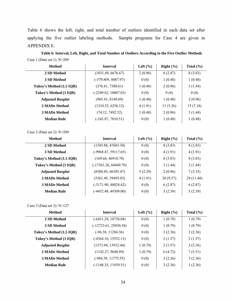
Table 6 shows the left, right, and total number of outliers identified in each data set after
applying the five outlier labeling methods. Sample programs for Case 4 are given in
APPENDIX E. Table 6: Interval, Left, Right, and Total Number of Outliers According to the Five Outlier Methods
Case 1 (Data set 1): N=209
Method Interval Left (%) Right (%) Total (%)
2 SD Method (1031.49, 6676.67) 2 (0.96) 6 (2.87) 8 (3.83)
3 SD Method (-379.809, 8087.97) 0 (0) 1 (0.48) 1 (0.48)
Tukey’s Method (1.5 IQR) (376.81, 7380.61) 1 (0.48) 2 (0.96) 3 (1.44)
Tukey’s Method (3 IQR) (-2249.62, 10007.03) 0 (0) 0 (0) 0 (0)
Adjusted Boxplot (905.41, 8149.69) 1 (0.48) 1 (0.48) 2 (0.96)
2 MADe Method (1310.52, 6256.12) 4 (1.91) 11 (5.26) 15 (7.18)
3 MADe Method (74.12, 7492.52) 1 (0.48) 2 (0.96) 3 (1.44)
Median Rule (-243.87, 7810.51) 0 (0) 1 (0.48) 1 (0.48)
Case 2 (Data set 2): N=209
Method Interval Left (%) Right (%) Total (%)
2 SD Method (1545.88, 47603.30) 0 (0) 8 (3.83) 8 (3.83)
3 SD Method (-9968.47, 59117.65) 0 (0) 4 (1.91) 4 (1.91)
Tukey’s Method (1.5 IQR) (169.66, 46918.78) 0 (0) 8 (3.83) 8 (3.83)
Tukey’s Method (3 IQR) (-17361.26, 64449.70) 0 (0) 3 (1.44) 3 (1.44)
Adjusted Boxplot (8580.85, 66385.47) 5 (2.39) 2 (0.96) 7 (3.35)
2 MADe Method (5361.49, 39495.03) 4 (1.91) 20 (9.57) 24 (11.48)
3 MADe Method (-3171.90, 48028.42) 0 (0) 6 (2.87) 6 (2.87)
Median Rule (-4452.48, 49309.00) 0 (0) 5 (2.39) 5 (2.39)
Case 3 (Data set 3): N=127
Method Interval Left (%) Right (%) Total (%)
2 SD Method (-6431.28, 18738.04) 0 (0) 1 (0.79) 1 (0.79)
3 SD Method (-12723.61, 25030.38) 0 (0) 1 (0.79) 1 (0.79)
Tukey’s Method (1.5 IQR) (-96.38, 11284.36) 0 (0) 3 (2.36) 3 (2.36)
Tukey’s Method (3 IQR) (-4364.16, 15552.13) 0 (0) 2 (1.57) 2 (1.57)
Adjusted Boxplot (1373.94, 13932.44) 1 (0.79) 2 (1.57) 3 (2.36)
2 MADe Method (1142.27, 9648.89) 1 (0.79) 6 (4.72) 7 (5.51)
3 MADe Method (-984.39, 11775.55) 0 (0) 3 (2.36) 3 (2.36)
Median Rule (-1148.35, 11939.51) 0 (0) 3 (2.36) 3 (2.36)

35
Table 6 (continued)
Case 4 (Data set 4): N=126
Method Interval Left (%) Right (%) Total (%)
2 SD Method (1181.67, 10079.91) 1 (0.79) 4 (3.17) 5 (3.97)
3 SD Method (-1042.89, 12304.47) 0 (0) 1 (0.79) 1 (0.79)
Tukey’s Method (1.5 IQR) (-64.67, 11216.31) 0 (0) 2 (1.59) 2 (1.59)
Tukey’s Method (3 IQR) (-4295.04, 15446.68) 0 (0) 1 (0.79) 1 (0.79)
Adjusted Boxplot (1375.92, 13793.89) 1 (0.79) 1 (0.79) 2 (1.59)
2 MADe Method (1139.14, 9600.99) 1 (0.79) 5 (3.97) 6 (4.76)
3 MADe Method (-976.33, 11716.45) 0 (0) 2 (1.59) 2 (1.59)
Median Rule (-1116.50, 11856.62) 0 (0) 2 (1.59) 2 (1.59)
Overall, the results of the applications show similar patterns to those in the simulation
study. First, when data are skewed, the difference of the average percentage of outliers between
the 2 SD method and the 2 MADe method increases. Second, the 2 MADe method classifies
more observations as outliers than any other method does. Third, in the mildly right skewed data
set, Case 2, in which the adjusted boxplot is utilized, the number of the left outliers is larger than
that of the right outliers. Finally, the interval of the Median rule is between Tukey’s method
with 1.5 IQR and Tukey’s method with 3 IQR.
As was shown in the results of Case 3 and Case 4, such methods with robust measures as
the MADe method, Tukey’s method, the Median rule, and the Adjusted Boxplot are less affected
by the extreme value than the SD method, and the interval of the SD method becomes much
narrower after the single extreme value is excluded form data set 3 than other methods. With
regard to the 2 SD method, while one observation is found in Case 3, five observations are
detected as outliers in Case 4. That is, when there is a large gap between extreme values and the
rest of values as shown in the data set 3, such outlier labeling methods with mean and standard
deviation as the SD method and Z-Score may not detect the possible outliers which other
methods could detect. In the case of the two skewness measures, i.e., classical and medcouple
skewness, classical skewness, unlike medcouple skewness, is highly affected by even a few
extreme values. The classical skewness in data set 3 was 9.25, but it decreased to 1.008 in data
set 4 with the most extreme value—which was included in the data set 3—excluded, whereas the
medcouple skewness decreased only a little.
36
6.0 RECOMMENDATIONS
Figure 11 shows a decision making flowchart at to which outlier labeling method can be used in
different data situations. First, it is necessary to understand the data characteristics (explore data
step). When a data set consists of such subgroups as sex and income, it may be necessary to
check if its research variables have different characteristics according to the subgroups. For
example, in the case of detecting outliers in the adult height variable, it may be necessary to
adjust for sex since the distribution of height can vary by sex. In such a case, an appropriate
approach may be to stratify by sex. All the labeling methods in this paper can be applicable if a
data set has a normal distribution without a possible masking problem or large gap between the
majority of the data and extreme values. If the data set has a normal distribution with a possible
masking problem or large gap between the majority of the data and extreme values, the Z-score
and SD method may be inappropriate to use since these methods are highly sensitive to extreme
values. The methods for the data whose distribution is symmetric but not normal, e.g., a
biomodal distribution, are beyond the purview of this study. Tukey’s method, the MADe
method, the Median rule, and the Adjusted Boxplot may be appropriate when a data set is
skewed, such as in a lognormal distribution; however, among these four methods, the Adjusted
Boxplot especially takes into account the skewness of the data32.

37
Modified Z-Score Z-Score Not applicable Adjusted Boxplot Tukey’s Method
Tukey’s Method Modified Z-Score MADe Method
MADe Method SD Method Median Rule
Median Rule Tukey’s Method
Adjusted Boxplot MADe Method
Median Rule
Adjusted Boxplot
Figure 11: Flowchart of Outlier Labeling Methods
SymmetricDistribution
Masking Problem /
Large Gap
Yes No
Normal Distribution
Yes No
Consideration for skewness
Yes No
Masking Problem/
Large Gap
Yes No
Start
Explore data
38
7.0 DISCUSSION AND CONCLUSIONS
As shown in the simulation study, each method has different measures to detect outliers and
shows different behaviors according to the skewness and sample size of the data. The SD
methods use less robust measures, such as the mean and standard deviation, which are highly
affected by extreme values. Thus, their intervals have a tendency to be inflated as the data
increases in skewness, and consequently the average percentages of outliers change less than
other types of methods such as the MADe, Tukey’s method and the Median rule. Three methods
such as the MADe, Tukey’s method and the Median rule show similar patterns in skewed data
since they employ robust measures to build their intervals. The total average percentages of
outliers for these methods increase when data are skewed. Although the basic idea of the
adjusted boxplot is similar to Tukey’s method, it is different in that the adjusted boxplot has
skewness measure to take into consideration. Thus, the total average percentage of outliers for
the adjusted boxplot seldom changes, even decreases very slightly, when data are skewed. In
addition, the range of the percentages declines more rapidly than other methods as the sample
size increases. The total average percentage of outliers for the method, consequently, becomes
smaller than other methods as data becomes skewed and the sample size gets large.
The simulation results reported in Table 5 may not be an exact index of the outlier
percentage for each method according to the skewness and the sample size of the data as the real-
world data may not follow the same distributions employed in the simulation study as was shown
in Chapter 5. However, understanding the general features which the methods show would be
helpful in choosing the outlier labeling methods in normal or skewed data.
There can be a gap between the majority and a small fraction of the data in a skewed data
set. In general, when the observations located in the small fraction apart from the majority of the
data are considered target outliers, the likelihood of defining them as outliers can increase as the
distance of the gap increases. However, if the gap is not large enough, detecting outliers may

39
have different results depending on the methods. In such a case, it may be hard to generalize
how large the gap in each method should be in order to identify the observations in the small
fraction as outliers since data are diversely distributed. Another method to detect outliers is the
formal test based on specific distribution assumptions. This test defines the target outliers first,
and then examines whether or not the outliers are true. Some formal tests may define all of the
observations in the small fraction as outliers, whereas others may define only some of the last
observations in the tail of data distribution as outliers. Selection of formal tests mainly depends
on the number and the type of target outliers and the type of data distribution.1 In the future,
formal tests in various distributions will be reviewed, compared, and discussed.

40
APPENDIX A
THE EXPECTATION, STANDARD DEVIATION AND SKEWNESS OF A
LOGNORMAL DISTRIBUTION
Let X denote a random variable having a lognormal distribution, and then its natural
logarithm, )log(XY = , has a normal distribution. Aitchison and Brown (1957) note that when
Y has mean value μ=)(YE , and variance 2)( σ=YVar , the expected value and standard
deviation of the original variable X are as follows:
)2
exp()(2σμ +=XE
)2exp()22exp()( 22 σμσμ +−+=XSTDEV
It is usually denoted by ),(~ 2σμLOGNX , i.e., ),(~ 2σμLOGNX if and only if
),(~)log( 2σμNXY = . The skewness of X can be denoted as follows:
1)exp(]2)[exp()( 22 −+= σσXSKEW
Simple example:
If X is a lognormal random variable with parameters μ and σ , its natural logarithm,
)log(XY = , follows N( μ , 2σ ) . When μ =0 and σ =1 forY , the corresponding mean, standard
deviation, and skewness of X can be determined from the following:
649.1)5.00exp()2
exp()(2
=+=+=σμXE

41
161.2)1exp()2exp()2exp()22exp()( 22 =−=+−+= σμσμXSTDEV
185.61)1exp(]2)1[exp(1)exp(]2)[exp()( 22 =−+=−+= σσXSKEW
We may compute the theoretical cutoff value of the SD method using this information. For
example, when a certain variable, X , follows )1,0(LOGN , the theoretical lower and upper cutoff
value of the 2 SD method in the variable are 1.649 ± 2*2.161.

42
APPENDIX B
MAXIMUM Z SCORES
Shiffler (1988) showed that the maximum Z-Score depends on sample size n . Let x1, x2 ,…,xn-
1,xn be an ordered random sample of size n from a population with unknown mean and variance,
and let 1−nx be zero. The sample variance of the sample is presented as follows:
1
)(1
2
2
−
−=∑=
n
xxS
n
ini
n
=11
)(1
1
222
1 1
22
−
−+=
−
− ∑∑ ∑−
== =
n
nxxx
n
nxxn
inni
n
i
n
iii
=nx
n
xn
n
ii 2
1
1
2
1+
−
∑−
=
= nx
n
xx
nn n
n
ini 2
1
1
21
2
)(
12
+−
−⋅
−− ∑
−
=−
= nx
Snn n
n
22
112
+⋅−−
−
Now, the Z-Score of the sample is maximized when nS is minimized. Here, when 21−nS is zero,
nS has the smallest value. That is, the maximum Z-Score can be presented as follows:
n
nn
n
n
Snxx
Sxx
Z)()(
max−
=−
=
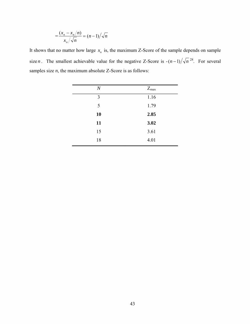
43
= nnnx
nxx
n
nn )1()(
−=−
It shows that no matter how large nx is, the maximum Z-Score of the sample depends on sample
size n . The smallest achievable value for the negative Z-Score is - nn )1( − 28. For several
samples size n, the maximum absolute Z-Score is as follows:
N Zmax
3 1.16
5 1.79
10 2.85
11 3.02
15
18
3.61
4.01
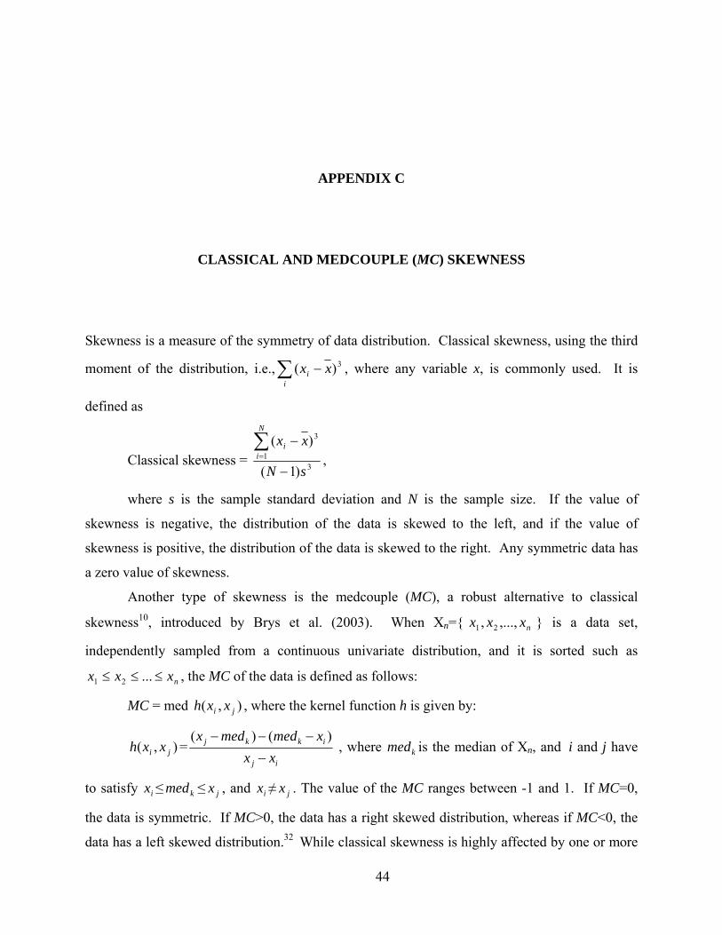
44
APPENDIX C
CLASSICAL AND MEDCOUPLE (MC) SKEWNESS
Skewness is a measure of the symmetry of data distribution. Classical skewness, using the third
moment of the distribution, i.e., 3)( xxi
i −∑ , where any variable x, is commonly used. It is
defined as
Classical skewness = 3
3
1
)1(
)(
sN
xxN
ii
−
−∑= ,
where s is the sample standard deviation and N is the sample size. If the value of
skewness is negative, the distribution of the data is skewed to the left, and if the value of
skewness is positive, the distribution of the data is skewed to the right. Any symmetric data has
a zero value of skewness.
Another type of skewness is the medcouple (MC), a robust alternative to classical
skewness10, introduced by Brys et al. (2003). When Xn={ nxxx ,...,, 21 } is a data set,
independently sampled from a continuous univariate distribution, and it is sorted such as
nxxx ≤≤≤ ...21 , the MC of the data is defined as follows:
MC = med ),( ji xxh , where the kernel function h is given by:
),( ji xxh =ij
ikkj
xxxmedmedx
−
−−− )()( , where kmed is the median of Xn, and i and j have
to satisfy ix ≤ kmed ≤ jx , and ix ≠ jx . The value of the MC ranges between -1 and 1. If MC=0,
the data is symmetric. If MC>0, the data has a right skewed distribution, whereas if MC<0, the
data has a left skewed distribution.32 While classical skewness is highly affected by one or more
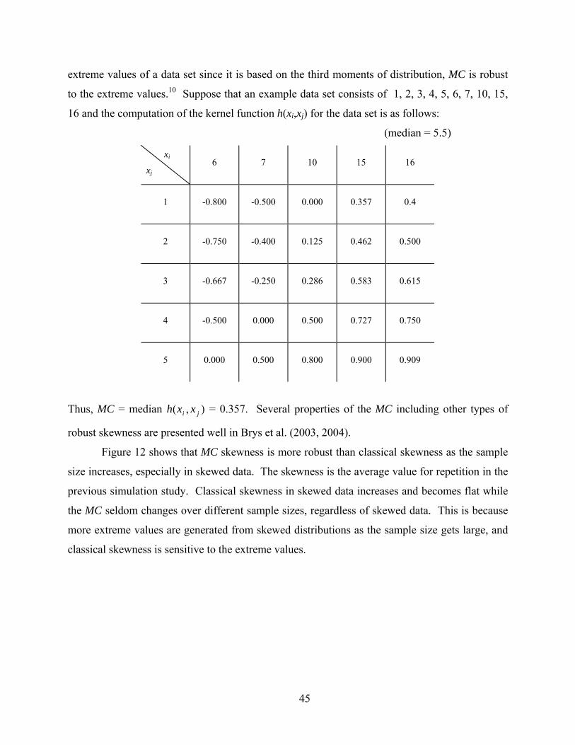
45
extreme values of a data set since it is based on the third moments of distribution, MC is robust
to the extreme values.10 Suppose that an example data set consists of 1, 2, 3, 4, 5, 6, 7, 10, 15,
16 and the computation of the kernel function h(xi,xj) for the data set is as follows:
(median = 5.5)
xi
xj 6 7 10 15 16
1 -0.800 -0.500 0.000 0.357 0.4
2 -0.750 -0.400 0.125 0.462 0.500
3 -0.667 -0.250 0.286 0.583 0.615
4 -0.500 0.000 0.500 0.727 0.750
5 0.000 0.500 0.800 0.900 0.909
Thus, MC = median ),( ji xxh = 0.357. Several properties of the MC including other types of
robust skewness are presented well in Brys et al. (2003, 2004).
Figure 12 shows that MC skewness is more robust than classical skewness as the sample
size increases, especially in skewed data. The skewness is the average value for repetition in the
previous simulation study. Classical skewness in skewed data increases and becomes flat while
the MC seldom changes over different sample sizes, regardless of skewed data. This is because
more extreme values are generated from skewed distributions as the sample size gets large, and
classical skewness is sensitive to the extreme values.

46
-0.5
0
0.5
1
1.5
2
2.5
3
3.5
4
4.5
0 200 400 600
sample size
cla
ssic
al skew
ness
SN
LN (0, 0.2)
LN (0, 0.4)
LN (0, 0.6)
LN (0, 0.8)
LN (0, 1.0)
-0.05
0
0.05
0.1
0.15
0.2
0.25
0.3
0.35
0.4
0.45
0 200 400 600
sample size
medcouple
skew
nes
SN
LN (0, 0.2)
LN (0, 0.4)
LN (0, 0.6)
LN (0, 0.8)
LN (0, 1.0)
Figure 12: Change of the Two Types of Skewness Coefficients According to the Sample Size and Data
Distribution. (Note: This results came from the previous simulation. All the values are in Table 5 )

47
APPENDIX D
BREAKDOWN POINT
The notion of breakdown point was introduced by Hodges (1967) and Hampel (1968, 1971). It
is a robustness measure of an estimator such as the mean and median or a related procedure
using the estimators. The breakdown point of an estimator generally can be defined as the largest
percentage of the data that can be changed into arbitrary values without distorting the estimator21.
For example, if even one observation of a univariate data set is moved to infinity, the estimators
of the data set such as the mean and variance go to infinity. Thus, the breakdown point of these
estimators is zero. In contrast, the breakdown point of the median is approximately 50% and it
varies slightly according whether the sample size n is odd or even. The exact breakdown point
of the median is 50(1-1/n) % and 50(1-2/n) % for odd sample size n and even sample size n,
respectively21. Therefore, if the breakdown point of an estimator is high, the estimator is robust.
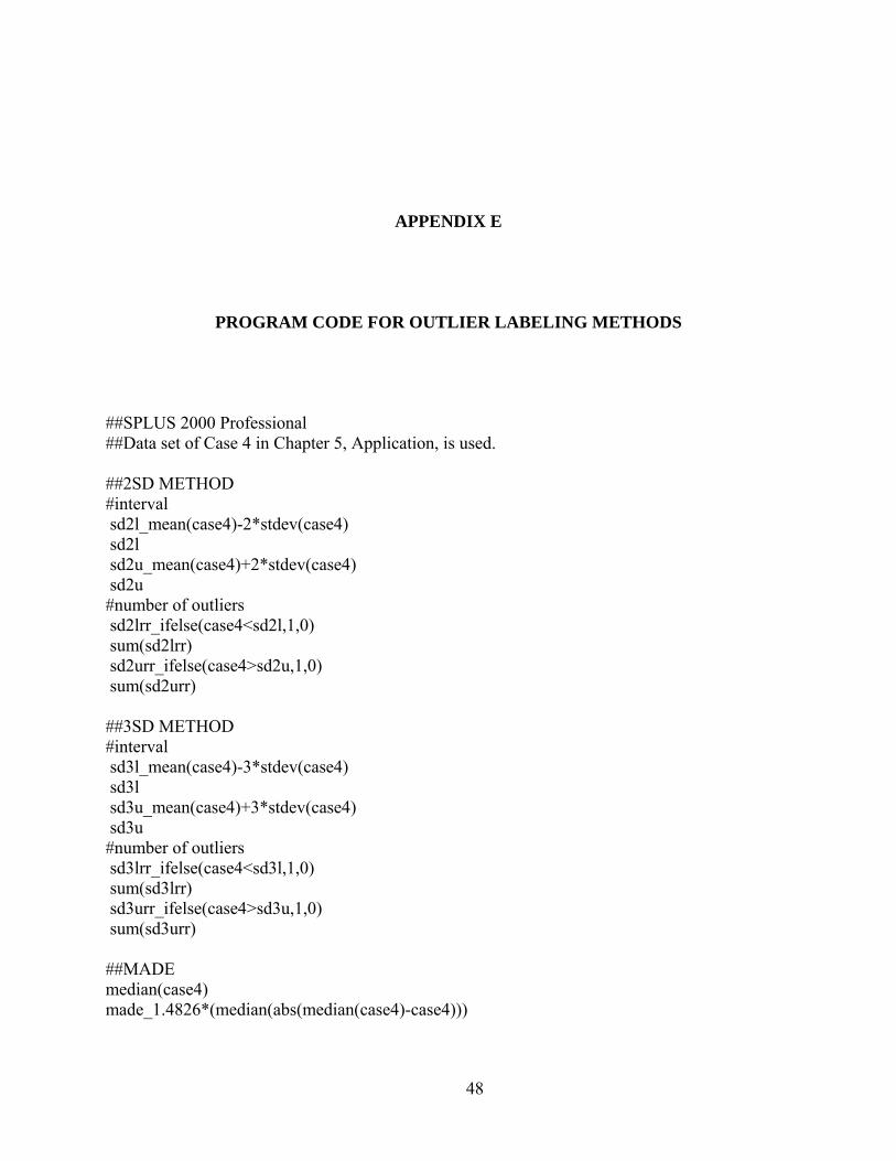
48
APPENDIX E
PROGRAM CODE FOR OUTLIER LABELING METHODS
##SPLUS 2000 Professional ##Data set of Case 4 in Chapter 5, Application, is used. ##2SD METHOD #interval sd2l_mean(case4)-2*stdev(case4) sd2l sd2u_mean(case4)+2*stdev(case4) sd2u #number of outliers sd2lrr_ifelse(case4<sd2l,1,0) sum(sd2lrr) sd2urr_ifelse(case4>sd2u,1,0) sum(sd2urr) ##3SD METHOD #interval sd3l_mean(case4)-3*stdev(case4) sd3l sd3u_mean(case4)+3*stdev(case4) sd3u #number of outliers sd3lrr_ifelse(case4<sd3l,1,0) sum(sd3lrr) sd3urr_ifelse(case4>sd3u,1,0) sum(sd3urr) ##MADE median(case4) made_1.4826*(median(abs(median(case4)-case4)))
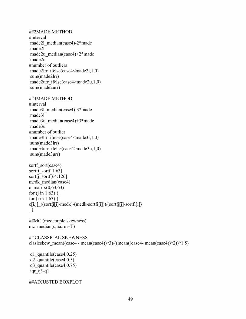
49
##2MADE METHOD #interval made2l_median(case4)-2*made made2l made2u_median(case4)+2*made made2u #number of outliers made2lrr_ifelse(case4<made2l,1,0) sum(made2lrr) made2urr_ifelse(case4>made2u,1,0) sum(made2urr) ##3MADE METHOD #interval made3l_median(case4)-3*made made3l made3u_median(case4)+3*made made3u #number of outlier made3lrr_ifelse(case4<made3l,1,0) sum(made3lrr) made3urr_ifelse(case4>made3u,1,0) sum(made3urr) sortf_sort(case4) sortfi_sortf[1:63] sortfj_sortf[64:126] medk_median(case4) c_matrix(0,63,63) for (j in 1:63) { for (i in 1:63) { c[i,j]_((sortfj[j]-medk)-(medk-sortfi[i]))/(sortfj[j]-sortfi[i]) }} ##MC (medcouple skewness) mc_median(c,na.rm=T) ## CLASSICAL SKEWNESS clasicskew_mean((case4 - mean(case4))^3)/((mean((case4- mean(case4))^2))^1.5) q1_quantile(case4,0.25) q2_quantile(case4,0.5) q3_quantile(case4,0.75) iqr_q3-q1 ##ADJUSTED BOXPLOT

50
#interval adjl_q1-1.5*exp(-3.5*mc)*iqr adjl adju_q3+1.5*exp(4*mc)*iqr adju #number of outliers adjlrr_ifelse(case4<adjl,1,0) sum(adjlrr) adjurr_ifelse(case4>adju,1,0) sum(adjurr) ## TUKEY’S METHOD #inner fence tukey1.5l_q1-1.5*iqr tukey1.5l tukey1.5u_q3+1.5*iqr tukey1.5u #outer fence tukey3l_q1-3*iqr tukey3l tukey3u_q3+3*iqr tukey3u #number of outliers (inner fence) tukey1.5lrr_ifelse(case4<tukey1.5l,1,0) sum(tukey1.5lrr) tukey1.5urr_ifelse(case4>tukey1.5u,1,0) sum(tukey1.5urr) #number of outliers (outer fence) tukey3lrr_ifelse(case4<tukey3l,1,0) sum(tukey3lrr) tukey3urr_ifelse(case4>tukey3u,1,0) sum(tukey3urr) ##MEDIAN RULE #interval medianl_q2-2.3*iqr medianl medianu_q2+2.3*iqr medianu #number of outliers medianlrr_ifelse(case4<medianl,1,0) sum(medianlrr) medianurr_ifelse(case4>medianu,1,0) sum(medianurr)

51
BIBLIOGRAPHY
1. Acuna, E., Rodriguez, C. A Meta analysis study of outlier detection methods in classification. Technical paper, Department of Mathematics, University of Puerto Rico at Mayaguez, 2004
2. Aitchison, J., J.A.C. Brown. The Lognormal distribution. Cambridge University Press, Cambridge, 1957
3. Bain, L., Engelhardt, M. Introduction to probability and mathematical statistics. 2nd ed., Duxbury, 1992
4. Barnett, V., Lewis, T. Outliers in statistical data. 3rd ed, Wiley, 1994
5. Bendre, SM., Kale, BK. Masking effect on test for outliers in normal sample. Biometrika, Vol. 74, No. 4 (Dec., 1987), 891-896
6. Ben-Gal, I. Outlier detection. Data Mining and Knowledge Discovery Handbook: A Complete Guide for Practitioners and Researchers, Kluwer Academic Publishers 2005.
7. Brandt, R. Comparing classical and resistant outlier rules. Journal of the American Statistical Association, Vol. 85, No. 412 (Dec., 1990), 1083-1090
8. Brys, G., Hubert, M., Rousseeuw, P.J. A robustification of independent component analysis. Journal of Chemometrics 2005
9. Brys, G., Hubert, M., Struyf, A. A Comparison of some new measures of skewness. Developments in Robust Statistics, ICORS 2001, eds. R. Dutter, P. Filzmoser, U. Gather and P.J. Rousseeuw, Springer-Verlag: Heidelberg, pp. 98-113:2003
10. Brys, G., Hubert, M., Struyf, A. A robust measure of skewness. Journal of Computational and Graphical Statistics 2004; 13: 996-1017
11. Burke, S. Missing values, outliers, robust statistics & non-parametric methods. LC.GC Europe Online Supplement, statistics and data analysis, 19-24
12. Carling, K. Resistant outlier rules and the non-Gaussian case. Computational statistics and data analysis, vol 33, 2000, pp 249-258.
52
13. Clark, J. Determining outliers. Hollins University, 2004, available at http://www1.hollins.edu/faculty/clarkjm/Stat140/Outliers.htm
14. Davies, L., Gather, U. The identification of multiple outliers. Journal of the American Statistical Association, Vol. 88, No. 423 (Sep., 1993), 782-792.
15. Hampel, FR. A general qualitative definition of robustness. Annals of Mathematical Statistics, 42, 1887-1896.
16. Hampel, FR. Contributions to the theory of robust estimation. Ph.D. Thesis, Dept. Statistics, Univ. California, Berkeley. 1968
17. Hartwig, F., Dearing, B.E. Exploratory data analysis. Newberry Park, CA: Sage Publications, Inc.;1979
18. Harvey, M. Prism statistics guide, version 4.0, 2003
19. High, R. Dealing with outliers: How to maintain your data’s integrity. University of Oregon, 2000, available at http://cc.uoregon.edu/spring2000/outliers.html
20. Hoaglin, D., Tukey, JW. Performance of some resistant rules for outlier labeling. Journal of the American Statistical Association, Vol. 81, No. 396 (Dec., 1986), 991-999
21. Iglewicz, B., Hoaglin, D. How to detect and handle outliers. ASQC Quality Press, 1993.
22. Lethen, J. Chebychev and empirical rules. Texas A&M University, 1996, available at http://stat.tamu.edu/stat30x/notes/node33.html
23. Marsh, GM. Standard protocol for outlier analysis of dissatisfaction Rate, Technical Report, University of Pittsburgh, 2002.
24. Meyer, RK., Krueger, D. A minitab guide to statistics. 2nd ed., Prentice Hall, 2001.
25. Olsson, U. Confidence interval for the mean of a lognormal distribution. Journal of Statistics Education, Vol. 13, No 1 (2005)
26. Osborne, JW., Overbay, A. The power of outliers (and why researchers should always check for them). Practical Assessment, Research & Evaluation, 9(6). 2004
27. Rosner, B. Fundamentals of biostatistics. 4th ed., Pacific Grove (CA), Duxbury, 1992.
28. Schiffler RE. Maximum Z Score and outliers. The American Statistician, Vol. 42, No.1 (Feb., 1988), 79-80
29. Siegel, A. Statistics and data analysis: An Introduction, Wiley, New York, 1988
30. Stephenson, D. Environmental statistics for climate researcher. University of reading, U.K., 2004

53
31. Tukey, JW. Exploratory data analysis. Addison-Wesely, 1977
32. Vanderviere, E., Huber, M. An adjusted boxplot for skewed distributions. Compstat 2004 graphics.
33. Zhou, X., Gao, S. Confidence intervals for the lognormal mean. Statistics in medicine, Vol. 16, 783-790, 1997