1

2

أهــــــداء

إلى الشموع التي ذابت في كبرياء لتنير كل خطوة في دربنا

لتذلل كل عائق أمامنا فكانوا رسالً للعلم واألخالق

شكراً لكم جميعاً اعضاء هيئة تدريس قسم الجيولوجيا جامعة اسيوط عامة واخص

د/ مصطفي ثابت والي روحح المغفور له باذن اهللا د/ ابوضيف عبدالعال بخيت

خالص حبي وتقديري حسين عبد الحفيظ مدبولي رابعه جيوفيزياء

3

Contents

1. Introduction …………………………………………………………..……….4-5

2. Geology of study area and surrounding parts……………….…………......6 -13

2.1 . Stratigraphic Framework……………………………………….….…6

2.2 . Structural Framework……………………………………….….…7-13

3 Electric investigation (DC Resistivity Method)……………………….…. 14-43

3.1 Resistivity Basics……………………………………………………14-18

3.2 Resistivity Surveys and Geology…………………………………..18-22

3.3 Resistivity Equipment and Field Procedures……………………..23-35

3.4 field work……………………………………………………………….36

3.5 Interpretation of Resistivity Measurements………………………37-41

3.5.1 RES2DINV ver. 3.59 Software………………………………….. 37-40

4 Summary and Conclusion………………………………...………....……..…..42

5 References………………………………………………………………..………43

4

1.Introduction

The study area is located at Wadi El-Nakheil, about 15 km to the west of Quseir

district, it lies between Latitudes 26° 5'30.42" and 26° 9'0.18"N and Longitudes 34° 11'

24"and 34° 8'26.93"E(Fig. 1). The study area represents one of the most promising areas

for land reclamation and future projects depending on groundwater for land irrigation and

human use. Therefore, this area was chosen by FAO as a part of a huge international

agricultural project. This project aims to use the vast desert areas for constructing new

villages for graduated youth. This area is characterized by vast plain close to Quseir

district and located close to the Qift-Quseir Desert Road. The major problem considered

in this area is the lack of sufficient and safe water supply.

Different geological and geophysical studies were carried out in the area and its

surrounding parts such as; Youssef (1957); Akkad &Dardir (1960); Ghanem et al.

(1970); Said (1990); Khalil &McClay (2002); A.Salemet al. (2005) andW.Sauck,

M.Sultan&A.Wagdy (2007); and many others.

The aim of the present study is to investigate the subsurface geological and

hydrogeological conditions. This includes;

1- Recognizing the different sedimentary layers as possible in this area.

2- Detecting the groundwater potentiality.

3- Identifying the structural characteristics of subsurface sequences.

5

Fig. 1: Location map for the study area

6

3. Geology of study area and surrounding parts

3.1 . Stratigraphic Framework

The stratigraphy of the northwestern margin of the Red Sea consists of

Precambrian crystalline basement (meta-volcanics, meta-sediments and granitoid

intrusives; Akaad and Noweir, 1980; Said, 1990) together with Mesozoic-Cenozoic

pre-rift sediments and Late Oligocene-Miocene to Recent syn-rift sediments (Fig. 2).

The basement contains strong fabrics (faults, fractures, shear zones and dykes)

oriented WNW, NNW, NS and ENE (Fig. 2). The basement is uncomfortably overlain

by a 500-700m thick section of pre-rift strata that ranges in age from the Late

Cretaceous to the Middle Eocene (Fig. 2). The lower part of the pre-rift section is the

130m massive, thick-bedded, siliciclastic Nubia Formation. This is overlain by a 220-

370m thick sequence of interbedded shales, sandstones and limestones of the Quseir,

Duwi, Dakhla and Esna Formations (Fig. 2; Youssef, 1957; Abd El-Razik, 1967;

Issawi et al., 1969). The uppermost pre-rift strata consist of 130-200m of competent,

thick-bedded limestones and cherty limestones of the Lower to Middle Eocene Thebes

Formation (Fig. 2).

The Late Oligocene to Recent syn-rift strata unconformably overlie the Thebes

Formation and vary in thickness from less than 100 m onshore to as much as 5 km in

offshore basins (Heath et al., 1998). The lowermost syn-rift strata are dominantly

coarse-grained clastics (Nakheil and Ranga Formations; Fig. 2). These clastics are

overlain by reef limestones, clastics and evaporites (Um Mahara, Sayateen and Abu

Dabbab Formations; Fig. 2). Late Miocene carbonates and reefs and Pliocene to

Recent syn-rift clastics overlie the evaporites in the coastal outcrops (Figs. 2 and 3;

Montenant et al., 1998; Plaziat et al., 1998).

7

3.2 . Structural Framework

The structure of the northwestern margin of the Red Sea is dominated by two

large, linked normal fault systems, the border fault system and the coastal fault system

(Fig. 2a), and includes part of the Duwi accommodation zone. This accommodation

zone appears to have been localized by the Precambrian Hamrawin shear zone

(Moustafa, 1997; Younes and McClay, 2001; Fig. 2a). In the northern part of the map

(Fig. 2), the major faults dip to the northeast. South of the prominent Precambrian

Hamrawin shear zone (Fig.3a), the fault polarities change and the fault dip is mainly to

the southwest (Fig. 2b). The coastal fault system dominantly trends NW and delineates

the main exposures of the syn-rift strata along the Red Sea coast (Fig. 2a). Here the

Anz fault segment (AF in Fig. 2a) dips NE but to the south, acrros the accommodation

zone, the Zug el Bahar fault segment dips SW (ZF in Fig. 2a). Minimum throws on the

coastal fault system vary from 0.5 to 2 km (based on topographic offset of the

basement and pre-rift strata).

The Border fault system is more complex. North and west of Hamrawin shear

zone it consists of the NE-dipping Kallahin fault (KF in Fig. 2a). South of the

Hamrawin shear zone the Border fault system dips to the SW and is strongly

segmented with two dominant faults; the Nakheil fault (NF in Fig. 2a) and the

Hamadat fault (HF in Fig. 2a). Both of these faults exhibit three major strike

directions, WNW, NW and N (Fig. 2a), and typically display a zig-zag pattern. The

hanging-wall structure of the border fault system is characterized by several large,

doubly-plunging, asymmetric hanging-wall synclines, the largest of which, the Gabal

Duwi structure, is over 40 km long (Fig. 2a). The hanging-wall of the Hamadat fault

also displays three prominent, but smaller, doubly-plunging synclines (Fig. 2a). In the

immediate hanging-wall of the Border fault system, the beds dip steeply sub-parallel to

the fault (Fig. 2b). Rare isolated outcrops of Late Oligocene syn-rift Nakheil sediments

are found in the core of the Duwi structure (Fig. 2a and 3b). In the map (Fig. 2a), the

estimated stratigraphic throw along the Border fault system varies from 1.5 to 3.5 km

(based on topographic offset against basement and offsets of the pre-rift strata).

8

Cross-sections through the Duwi and Hamadat areas show that the Border fault

system bounds a series of WNW- and NW-trending half grabens whose average width

is 8 km and average bed dip is 15° towards the northeast (Fig. 2b). The half grabens

are cut by smaller displacement faults into 1-3 km wide, domino-style fault blocks.

These smaller faults dip 55-65° and have stratigraphic throws that range from tens to a

few hundreds of meters (Fig.3b).

The Duwi map area is dominated by the massive outcrops of the Eocene Thebes

limestone that form parts of the large complex, asymmetric syncline systems of the

hanging wall of the Nakheil fault system (Fig.4). The footwall of the Nakheil fault

system consists dominantly of Precambrian basement (including the Hamrawin

granite; Fig.4a) except in the southern sections where gentle, moderately east-dipping

Nubia sandstones occur in the footwall (Fig. 4b).

Although the overall strike of the Nakheil fault system is NW, in detail the fault

system is strongly segmented with NW-, WNW- and NS-striking sections (Fig. 4a).

These dip 58-66° SW and have minimum stratigraphic offsets of 1.5-2.3 km. There are

two distinct relay ramps (using the terminology of Larsen, 1988; Peacock and

Sanderson, 1991; Peacock et al., 2000) that link what appear to be originally separate

segments of the Nakheil fault system (Fig.4a). There are four distinct, offset, NW-

trending, hanging-wall synclines in the Duwi area (Fig.4a). The northernmost, SE-

plunging syncline is outlined by the massive outcrops of Thebes limestones and occurs

in the hanging wall of the NE-dipping Kallahin fault, in the zone of transfer between it

and the SW-dipping Nakheil fault system (Fig. 4a).

The main northern Nakheil syncline is some 23 km long and has a curvilinear

axial-surface trace, merging with the Kallahin syncline at its northwestern end (Fig.

4a).

9

Its southern termination is a complex of en echelon normal faults where the

syncline plunges gently to the north. The axial trace of the northern syncline has two

bends localized by the Hamrawin granite and the relay ramp R1 (Fig. 4a). The doubly-

plunging, central and southern Nakheil hanging-wall synclines are associated with

separate NW- and N-trending Nakheil fault segments (Fig. 4a).

The central and southern synclines are offset through a NS-trending fault that cuts

across Wadi El Nakheil (Fig. 4a). The Nakheil synclines are noticeably asymmetric

with gently (12-19°) E- and NE-dipping limbs and steep (30-60°) W-SW-dipping limbs

(Fig. 4b). The E-NE-dipping limbs decrease in dip to only 7-9°further westwards away

from the influence of the Nakheil fault. The panels of W-SW-dipping strata vary from

0.5 to 2km in width. The width of the steep limb adjacent to the fault decreases with

depth and appears to be absent at the top of the Precambrian basement and Nubia

sandstones. Where the faults cut through basement and the massive to thick-bedded

Nubia sandstones, footwall and hanging-wall deformation is localized to a few meters

either side of the fault and no significant footwall or hanging wall folding is found.

The NE-SW-oriented cross-sections show that the structural relief of the northern and

central synclines is about 2 km and the wavelength is 5-6 km.

10

Fig. 2a: Simplified geologic map of Gabal Duwi-Gabal Hamadat area, northwestern Red Sea. KF, NF

and HF indicate the Kallahin, Nakheil and Hamadat fault segments of the Border fault system,

respectively, and AF and ZF indicate the Anz and Zug El Bahar fault segments of the coastal fault

system. (From Khalil and McClay, 2002)

Fig. 2b: Regional cross-sections across the Gabal Duwi-Gabal Hamadat area (location are shown in

(a)). (From Khalil and McClay, 2002)

11

Fig. 2: Summary stratigraphy of the northwestern Red Sea rift system. Data from Said

(1990), Purser and Bosence (1998), and Khalil &McClay (2002).

12

13

Fig.4b: Structural cross-sections across Gabal Duwi area (locations are shown in

(a)).(From Khalil and McClay, 2002)

14

3. Electric investigation (DC Resistivity Method) 3.1 Resistivity Basics 3.2 Resistivity Surveys and Geology 3.3 Resistivity Equipment and Field Procedures 3.4 field work 3.5 Interpretation of Resistivity Measurements

3.1 Resistivity Basics

Current flow and Ohm’s law

V=IR

Resistivity vs. Resistance

15

Resistivity of Earth Materials

16

Current Densities and Equipotential

A First Estimate of Resistivity

17

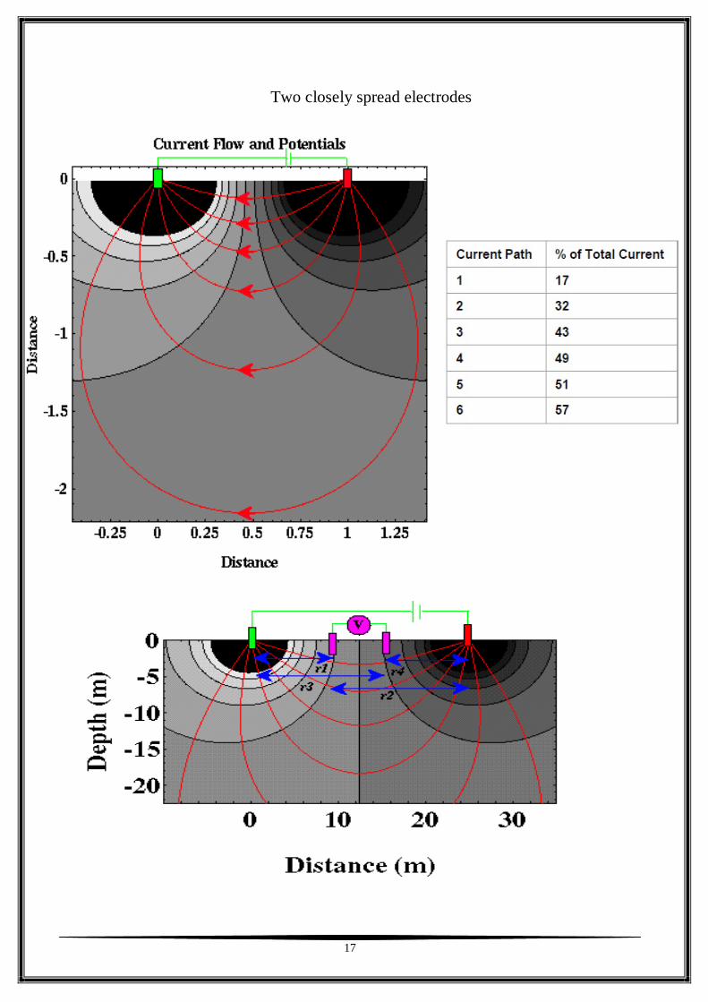
Two closely spread electrodes

A practical way of measuring resistivity

18

A practical way of measuring resistivity

3.2Resistivity Survey and Geology

Sources of Noise Depth of Current Penetration vs. Current Electrode Spacing Current Flow in Layered Media Variation in Apparent Resistivity: Layered vs. Homogeneous Media

19

Sources of Noise

1-Electrode polarization a -Use nonpolarizing electrodes b -Use a slowly varying AC current 2-Telluric currents 3-Presence of nearby conductors 4-Low resistivity at the near surface 5-Near-electrode geology and topography

6-Current induction in measurement cables.

Depth of current penetration vs. current electrode spacing

Current flow in two layer media

20

Current distribution

Variation in Apparent Resistivity: Layered vs. Homogeneous Media

21

Current flow in layered media-Case 1

22

Current flow in layered media-Case 2

23

3.3 Resistivity Equipment and Field Procedure Equipment Survey Types Overview a- Soundings b- Profiles c- Tomography Choice of Best Array

Equipment DC Resistivity Equipment Current source Ammeter Voltmeter Electrodes Cables

Survey Types Overview Resistivity Soundings

To look for variations in resistivity with depth Resistivity Profiles

To detect lateral variations in resistivity Resistivity Tomography 2-D resistivity tomogram

Resistivity Soundings-

Pole-Pole Array

Pole-Pole sounding data is plotted as apparent resistivity vs. a

24

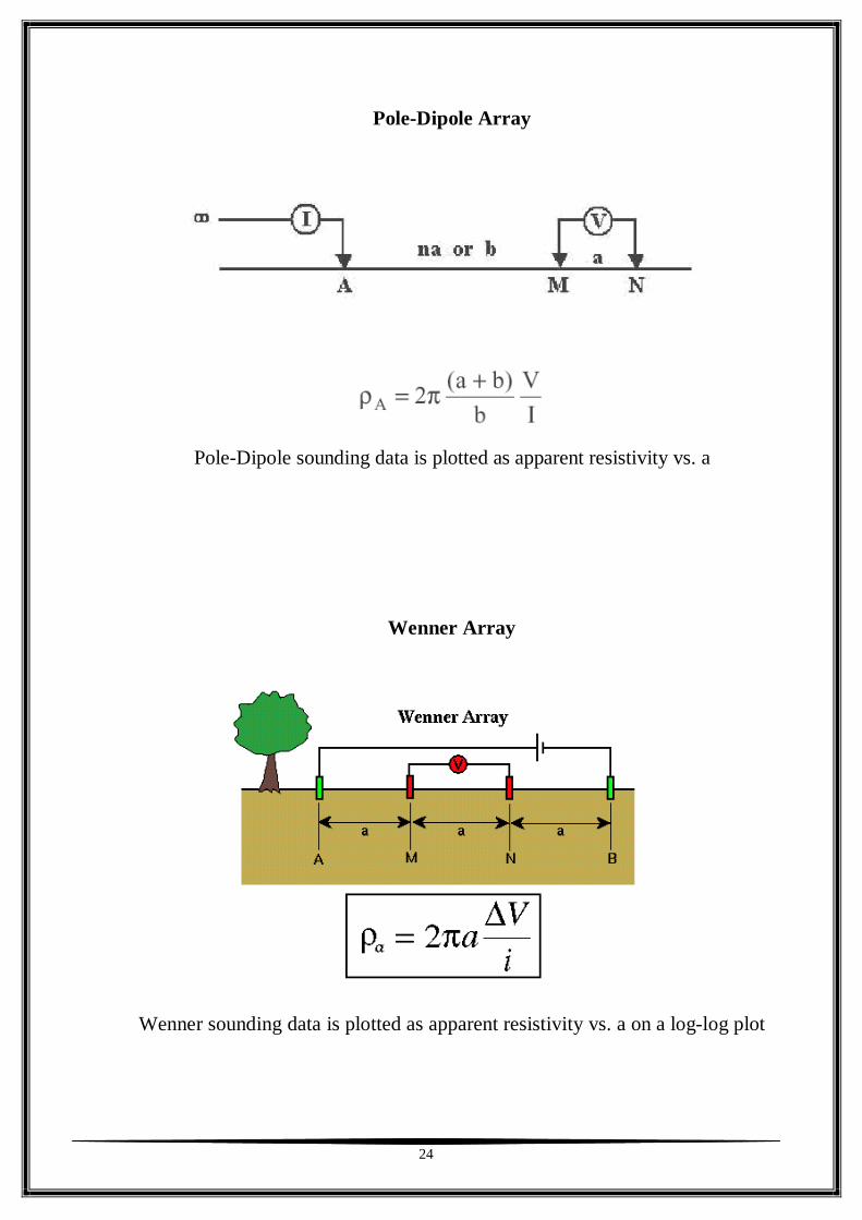
Pole-Dipole Array

Pole-Dipole sounding data is plotted as apparent resistivity vs. a

Wenner Array

Wenner sounding data is plotted as apparent resistivity vs. a on a log-log plot

25

Schlumberger Array

Schlumberger sounding data is plotted as apparent resistivity vs. s (AB/2) on a log-log plot

]Dipole-Dipole Array

Dipole-Dipole sounding data is plotted as apparent resistivity vs. s (AB/2) on a log-log plot

26

Electrode Spacings and Apparent Resistivity Plots

Resistivity Profiles

27

Resistivity Tomography

28

Pseudosection

CHOICE OF THE “BEST” ARRAY

Depends on: 1) type of structure to be mapped 2) sensitivity of the resistivity meter 3) background noise level

Things to be considered: 1) depth of investigation 2) sensitivity of the array to vertical and horizontal structures 3) horizontal data coverage

4) signal strength

29

Schlumberger Array

PARAMETERS CONTROLLING THE DEPTH OF INVESTIGATION On a theoretical point of view, the depth of investigation of a measurement depends on the length of the transmitting line AB and on the separation between the transmitting AB line and the receiving MN line. Various types of electrode combinations can be used (Schlumberger, Wenner, dipole, pole, gradient arrays, …), each of them featuring various benefits and limitations in terms of vertical penetration, lateral resolutions, field set-up, but all following the same general rules: the larger the length AB, the deeper the penetration of the current the farther the M, N receiving electrodes from the A, B transmitting electrodes,

the more representative the potential measured on the surface of the ground, of the resistivity of deep layers.

The arrays can be used on a sounding procedure where the depth of investigation is increased at each new reading for a given midpoint, or in a profiling procedure where the spacings between the electrodes is kept constant for all readings, the midpoint of the array being moved of an elementary distance at each new reading. In the profiling

30

procedure, the depth of investigation of the readings is determined by the spacings between the electrodes. On a practical point of view, the depth on investigation also depends on the measurability of the VMN potential which can be expressed as VMN = rho x IAB / K. For large investigation depths, the electrodes have to be far away from each other, the K coefficient has thus an important value, and the VMN signal becomes small, possibly difficult to measure. Several factors facilitate a good measurement at large investigation depths: a high ground resistivity “rho”: a 1000 ohm.m ground (hard rock) produces a

VMN signal ten times greater than a 100 ohm.m ground (sedimentary rock) and a hundred times greater than a 10 ohm.m ground (clayey formation). The resistivity parameter, linked to the nature of the rocks, is of course out of the control of the operator

a high intensity of the current IAB = VAB / RAB, which means:

• a low ground resistance RAB: if the surface layer is a dry sand (which has a very high resistivity), the ground resistance of the A and B electrodes are higher than if it is a clayey soil (which has a very low resistivity). However, it is possible to decrease a ground resistance RAB by using several long stakes at each A and B transmitting points, poured with salt water for instance, which decreases the resistivity of the ground located near to these transmitting points, thus the ground resistance RAB.

• and/or a high output voltage VAB,obtained with a powerful equipment. The resistivity systems are usually characterized by a maximum current, a maximum voltage and a maximum power, one of these three parameters determining the intensity of the current which can really be transmitted into the ground, in relation with the value of the ground resistance RAB.

a highly sensitive meter, with filtering capability including stacking / averaging process for noise rejection (Self Potential, drift of SP, power lines fields, other industrial or natural electromagnetic interferences,…), which makes it possible to measure a low VMN amplitude in an as-short-as-possible acquisition time.

31

In case of a two layer sounding, when the second layer is more resistive than the first one, its presence is observed in the apparent resistivity curve for a length of line AB/2 longer than when the second layer is more conductive. In the figure, XR is longer than XC, for the same relative variation of the apparent resistivity curve

32

DEPTH OF INVESTIGATION OF VERTICAL ELECTRICAL SOUNDING (VES)

In the VES technique, the ground is supposed to be composed of horizontal layers. It is a common rule of thumb to say that the depth of investigation is of the order of 0.1 to 0.3 times the AB length: a 1km AB line leads to a depth of 100 to 300m, depending on the type of layering (for instance, aconductive basement can be seen with a shorter AB line than a resistive one; however, the signal is normally lower in the first case than in the second one). In a traditional Sclumberger or Wenner electrical sounding, the transmitting A and B electrodes are successively moved away from each other at each new reading to increase the depth of investigation. The operator fully controls the AB and MN lengths, as the four electrodes and their wires are independent. As the time necessary to move from one position to the next one becomes longer and longer for deep investigations, it is reasonable in these soundings to spend a significant time to stack the signal so as to improve the quality of the reading or to make this reading possible.

33

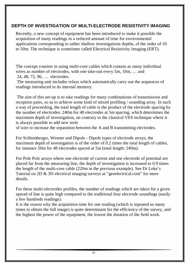
DEPTH OF INVESTIGATION OF MULTI-ELECTRODE RESISTIVITY IMAGING

Recently, a new concept of equipment has been introduced to make it possible the acquisition of many readings in a reduced amount of time for environmental applications corresponding to rather shallow investigations depths, of the order of 10 to 50m. The technique is sometimes called Electrical Resistivity Imaging (ERT).

The concept consists in using multi-core cables which contain as many individual wires as number of electrodes, with one take-out every 5m, 10m, … and 24, 48, 72, 96, … electrodes. The measuring unit includes relays which automatically carry out the sequences of readings introduced in its internal memory. The aim of this set-up is to take readings for many combinations of transmission and reception pairs, so as to achieve some kind of mixed profiling / sounding array. In such a way of proceeding, the total length of cable is the product of the electrode spacing by the number of electrodes: 240m for 48 electrodes at 5m spacing, which determines the maximum depth of investigation, on contrary to the classical VES technique where it is always possible to add new reels of wire to increase the separation between the A and B transmitting electrodes. For Schlumberger, Wenner and Dipole - Dipole types of electrode arrays, the maximum depth of investigation is of the order of 0.2 times the total length of cables, for instance 50m for 48 electrodes spaced at 5m (total length: 240m). For Pole Pole arrays where one electrode of current and one electrode of potential are placed far from the measuring line, the depth of investigation is increased to 0.9 times the length of the multi-core cable (220m in the previous example). See Dr Loke’s Tutorial on 2D & 3D electrical imaging surveys at “geoelectrical.com” for more details. For these multi-electrodes profiles, the number of readings which are taken for a given spread of line is quite high compared to the traditional four electrode soundings (easily a few hundreds readings). It is the reason why the acquisition time for one reading (which is repeated so many times to obtain the full image) is quite determinant for the efficiency of the survey, and the highest the power of the equipment, the lowest the duration of the field work.

34

DEPTH OF INVESTIGATION OF MULTI-ELECTRODE RESISTIVITY IMAGING WITH ROLL ALONG EXTENSIONS

The maximum depths here above mentioned are obtained when the electrodes located at the extremity of the line are addressed. This corresponds to one only point which is the middle point of the array. When the line to prospect is longer than the length of the multi-core cable, a roll along procedure is usually used where the first segment of the multi-core cable is moved to the extremity of the cable to enable further readings. For instance, if a 48 electrode 240m long initial line consists in two segments of 120m with 24 electrodes spaced at 5m for each segment, the minimum displacement consists in one segment of 120m. This makes that the continuity of the image will be only ensured for half the maximum depth of the array as reported in the previous paragraph (see figure 3 for visual understanding).

35

36

3.4. Field Work

In this study, resistivity measurements along one profiles as five spreads (A-C , B-D , C-E , D-F and E-G ) were carried out during Red Sea student field trip

(From 5April to 14April, 2013)

AB APPARENT RESISTIVITY

AB APPARENT RESISTIVITY

AB APPARENT RESISTIVITY

AB APPARENT RESISTIVITY

AB APPARENT RESISTIVITY

3 246.80 3 1306.24 3 248.69 3 614.81 3 63.24 4 228.44 4 932.58 4 373.27 4 687.66 4 70.77 6 181.34 6 582.47 6 385.20 6 1107.24 6 43.96 8 163.20 8 648.85 8 375.86 8 1864.45 8 418.39 6 171.44 6 658.14 6 374.29 6 1007.31 6 256.22 8 153.08 8 555.78 8 383.16 8 1224.60 8 916.10

10 164.66 10 403.93 10 423.90 10 1755.89 10 972.14 14 261.50 14 378.31 14 822.93 14 3564.53 14 471.00 18 395.64 18 1701.88 18 1111.56 18 624.23 18 1161.80 24 718.43 24 28.06 24 162.77 24 797.01 24 1329.10 18 109.65 18 14.32 18 13.00 18 134.52 18 64.06 24 149.78 24 279.07 24 301.68 24 289.67 24 74.18 30 245.30 30 42.96 30 435.20 30 895.28 30 146.95 40 439.94 40 34.79 40 941.27 40 240.43 40 306.94 30 22.61 30 142.56 30 503.66 30 571.48 30 106.76 40 32.38 40 244.92 40 1083.30 40 259.05 40 176.63 60 35.72 60 153.86 60 2148.55 60 3577.25 60 467.08 80 34.62 80 296.73 80 3808.04 80 107.32 80 642.92 60 34.29 60 212.88 60 642.92 60 1338.69 60 542.91 80 31.80 80 2480.22 80 1205.66 80 53.26 80 2149.00

100 33.76 100 645.63 100 1675.27 100 221.54 100 3764.07 140 67.25 140 1403.88 140 4791.69 140 462.36 140 1597.23 180 55.95 180 2350.10 180 8141.42 180 1748.59 180 18339.19 240 49757.57 240 4196.42 240 13163.77 240 1810.96 240 11989.78 180 1281.12 180 82.90 180 76.11 180 527.52 180 174.08 240 2543.40 240 190.76 240 25080.75 240 105.98 240 441.56 300 3617.28 300 1073.88 300 59232.96 300 1073.88 300 678.24 400 6179.62 400 2148.55 400 154695.24 400 6179.62 400 1278.90

37

3.5 Interpretation

3.5.1 RES2DINV ver. 3.59 Software

3.5.1.1 Introduction

RES2DINV is acomputer program that will automatically determine a two dimensional (2-D) resistivity model for the subsurface for the data obtained from electrical imaging surveys (Griffiths and Barker 1993). Since it is a Windows based program, all Windows compatible graphics cards and printers are automatically supported. It has been tested with video screen modes of up to 1600 by 1200 pixels and 16 million colours.

The 2-D model used by the inversion program, which consists of a number of rectangular blocks, is shown in Figure. The arrangement of the blocks is loosely tied to the distribution of the data points in the pseudosection. The distribution and size of the blocks is automatically generated by the program using the distribution of the data points as a rough guide. The depth of the bottom row of blocks is set to be approximately equal to the equivalent depth of investigation (Edwards 1977) of the data points with the largest electrode spacing. The survey is usually carried out with a system where the electrodes are arranged along a line with a constant spacing between adjacent electrodes. However, the program can also handle data sets with a non-uniform electrode spacing. A forward modelling subroutine is used to calculate the apparent resistivity values, and a non-linear least-squares optimisation technique is used for the inversion routine (deGroot-Hedlin and Constable 1990, Loke and Barker 1996a). The program supports both the finite-difference and finite-element forward modelling techniques. This program can be used for surveys using the Wenner, pole-pole, dipole-dipole, pole-dipole, Wenner-Schlumberger and equatorial dipole-dipole (rectangular) arrays. In addition to these common arrays, the program even supports non-conventional arrays with an almost unlimited number of possible electrode configurations! You can process pseudosections with up to 16000 electrodes and 21000 data points at a single time on a computer with 1 GB RAM. The largest electrode spacing can be up to 36 times the smallest spacing used in a single data set. The program data limits will be extended in the future as larger field data sets are encountered. Besides normal surveys carried out with the electrodes on the ground surface, the program also supports underwater and cross-borehole surveys!

38

Figure 6.Sequence of measurements to build up a pseudosection using a

computer controlled multi-electrode survey setup.

Figure 7. Arrangement of the blocks used in a model together with the data points in the pseudosection.

39

3.5.1.2 Theory

The inversion routine used by the program is based on the smoothnes- constrained least-squares method (deGroot-Hedlin and Constable 1990, Sasaki 1992). The smoothness-constrained least-squares method is based on the following equation JTJ + uF)d = JTg (1) Where F = fxfxT + fz fz T fx = horizontal flatness filter fz = vertical flatness filter J = matrix of partial derivatives u = damping factor d = model perturbation vector g = discrepancy vector One advantage of this method is that the damping factor and flatness filters can be adjusted to suit different types of data. A detailed description of the different variations of the smoothness-constrained least-squares method can be found in the free tutorial notes by Loke (2001). The program supports a new implementation of the least-squares method based on a quasi-Newton optimization technique (Loke and Barker 1996a). This technique is significantly faster than the conventional least-squares method for large data sets and requires less memory. You can also use the conventional Gauss-Newton method in this program. It is much than the quasi-Newton method, but in areas with large resistivity contrasts of greater than 10:1, it gives slightly better results. A third option in this program is to use the Gauss-Newton method for the first 2 or 3 iterations, after which the quasi-Newton method is used. In many cases, this provides the best compromise (Loke and Dahlin 2002). Due to improvements in the program code and PCs it is recommended that the option to use the Gauss-Newton method should be the default method, particularly for the final interpretation model, as for most data sets, the data inversion take only minutes on modern PC systems. The 2-D model used by this program divides the subsurface into a number of rectangular blocks (Figure 2). The purpose of this program is to determine the resistivity of the rectangular blocks that will produce an apparent resistivity pseudosection that agrees with the actual measurements. For the Wenner and Schlumberger arrays, the thickness of the first layer of blocks is set at 0.5 times the electrode spacing. For the pole-pole, dipole-dipole and pole-dipole arrays, the thickness is set to about 0.9, 0.3 and 0.6 times the electrode spacing respectively. The thickness of each subsequent deeper layer is normally increased by 10% (or 25%). The depths of the layers can also be changed manually by the user.

40

The optimization method basically tries to reduce the difference between the calculated and measured apparent resistivity values by adjusting the resistivity of the model blocks. A measure of this difference is given by the root-meansquared (RMS) error. However the model with the lowest possible RMS error can sometimes show large and unrealistic variations in the model resistivity values and might not always be the "best" model from a geological perspective. In general the most prudent approach is to choose the model at the iteration after which the RMS error does not change significantly. This usually occurs between the 3rd and 5th iterations. More information about the inversion method can be found in the free “Tutorial Notes” on electrical imaging (Tutorial : 2-D and 3-D electrical imaging surveys) that is available on the www.geoelectrical.com web site.

Fig (8) : example of 2D inversion cross section

41

(a)

Ohm.m

(b)

m/sec

Fig.(a) : The resulted 2D Resistivity profile at Wadi El-Nakheil

Fig.(b) : Corresponding 2D seismic Profile

0 7000

14000

21000

28000

35000

42

4 Summary and Conclusion

The study area is located west to Quseir district in the central Eastern Desert. It

lies between Latitudes 26° 5'30.42"and 26° 9'0.18"Nand Longitudes 34° 11' 24"and

34° 8'26.93"E. The study area represents one of the most promising areas for land

reclamation and future projects depending on groundwater for land irrigation and

human use. Therefore, this area was chosen by FAO as a part of a huge international

agricultural project. This project aims to use the vast desert areas for constructing new

villages for graduated youth.

Analysis of the obtained electric sections represented in the resistivity model,

structural models and the geoseismic cross-sections indicate that,

subsurface sections seem to have strong anisotropic medium in both vertical and

lateral directions.

Some lateral lithological variation is also noted along the distance 160m, where

the basement is adjacent to dipping underlying strata. This variation is indicated

as lateral change in the resistivity.

Also, there is a lateral variation where a lenticular body is adjacent to the beds.

The dipping underlying layers have SW dipping direction.,and with helping of

the nearest borehole in the area

The expected water-bearing formation is found at a depth ranges from about 30

to 65 m. The thickness of this layer ranges from 20-55 m/s. This layer has SW

dipping direction.

There is an angular disconformity between upper horizontal layers and the lower

dipping strata.

Also, a disconformity is noted between the surface Quaternary deposits and the

oligocene horizontal layer.

43

The area constitutes a wide flat area surrounded by numerous hills and terraces

of different elevations and the plain is covered by the Quaternary sediments.

44

4 – References

1) Zohdy, A. A. R., Eaton, G. P and Mabey, D.R. (1974) :Application of surface

geophysic, United States Government Office, Washington,

2) RES2DINV ver. 3.54 (2004), “Rapid 2-D Resistivity & IP inversion using the least-squares method”, GEOTOMO SOFTWARE Malaysia

3) S.M. Khalil , K.R. McClay,(2002), “Extensional fault-related folding, northwestern Red Sea” , Journal of Structural Geology 24 (2002) 743-762

4) A.Abd Elmaksoud, M. Elbhery (2013), “Studying The Upper Part Of The Subsurface Geologic Section In Wadi El-Nakeil, Eastern Desert , Egypt ”, 4th geophysics , Faculty of Science , Geology Department , Assiut University