a renewed analysis of cheating in contests: theory and
TRANSCRIPT

HAL Id: halshs-01059600https://halshs.archives-ouvertes.fr/halshs-01059600v2
Preprint submitted on 3 Sep 2015
HAL is a multi-disciplinary open accessarchive for the deposit and dissemination of sci-entific research documents, whether they are pub-lished or not. The documents may come fromteaching and research institutions in France orabroad, or from public or private research centers.
L’archive ouverte pluridisciplinaire HAL, estdestinée au dépôt et à la diffusion de documentsscientifiques de niveau recherche, publiés ou non,émanant des établissements d’enseignement et derecherche français ou étrangers, des laboratoirespublics ou privés.
A Renewed Analysis of Cheating in Contests: Theoryand Evidence from Recovery Doping
Sebastian Bervoets, Bruno Decreuse, Mathieu Faure
To cite this version:Sebastian Bervoets, Bruno Decreuse, Mathieu Faure. A Renewed Analysis of Cheating in Contests:Theory and Evidence from Recovery Doping. 2015. �halshs-01059600v2�

Working Papers / Documents de travail
WP 2014 - Nr 41
A Renewed Analysis of Cheating in Contests: Theory and Evidence from Recovery Doping
Sebastian BervoetsBruno Decreuse
Mathieu Faure

A renewed analysis of cheating in contests: theory
and evidence from recovery doping ∗
Sebastian Bervoets† Bruno Decreuse† Mathieu Faure†
June 2015
Abstract
In rank-order tournaments, players have incentives to cheat in order to
increase their probability of winning the prize. Usually, cheating is seen as
a technology that allows individuals to illegally increase their best potential
performances. This paper argues that cheating can alternatively be seen as a
technology that ensures that the best performances are reached more often. We
call this technology recovery doping and show that it yields new insights on the
effects of cheating: recovery doping lowers performance uncertainty, thereby
changing the outcome of the contest in favour of the best players. We develop
this theory in a game with player heterogeneity and performance uncertainty
and then study the results of the cross-country skiing World Cup between 1987
and 2006. In line with our theoretical predictions, race-specific rankings were
remarkably stable during the 1990s, subsequently becoming more volatile. This
pattern reflects the rise and fall of synthetic EPO and the emergence of blood
testing and profiling.
Keywords: Game theory; Recovery doping; Rank correlation
∗We thank Gerard Dine as well as the many people we interacted with on this project andseminar participants in Aix-Marseille University and Linnaeus University. We also thank LaurenceBouvard for her excellent research assistance.†Aix-Marseille University (Aix-Marseille School of Economics), CNRS and EHESS. Centre de
la Vieille Charite, 2 rue de la Charite, 13002 Marseille, France. The authors thank the FrenchNational Research Agency (ANR) for their support through the program ANR 13 JSH1 0009 01,as well as the Fondation Aix-Marseille Unversity and its program ”Sport, sante et developpementdurable”.
1

Individuals or institutions engaged in contest-like situations have incentive to use
illegal methods to increase their payments. Hedging funds compete for savings and
may practice fraudulent accounting to appear better than they are. Scientists may
voluntarily alter their datasets to enhance their results. And professional athletes
may take performance-enhancing drugs (PED) to outperform their opponents.
Cheating can take various forms. Usually, it is seen as a technology that allows
individuals to perform at super-natural levels, by illegally increasing their best po-
tential performances. Throughout the paper we refer to this effect as the standard
effect and because our main example will be sports, we call this cheating technol-
ogy doping. Here, we take a different angle, arguing that cheating can be seen as
a technology that ensures that the best performances are reached more often. To
pursue the analogy with sports, we call this particular technology recovery doping
and its effect the recovery effect.
Modeling the standard effect leads to the classical prisoner’s dilemma, where
competitors are forced into doping by a dominant strategy argument, but where all
competitors suffer due to the potential for cheating. They are trapped into a bad
equilibrium. Accounting for the recovery effect renews the analysis of cheating in
contests. While less talented agents suffer from the existence of cheating possibilities,
the most talented agents actually benefit from it. As they become more likely to
compete at their best level, they outperform the others more often. Recovery doping
therefore lowers contest uncertainty in favor of top agents. This has implications
for agents’ strategies, reward inequality and anti-cheating policies.
Though our model extends to different markets, we use high-level endurance
sports as our illustrating example, for several reasons. Top athletes are rational
players with the clear objective of maximizing their payoffs, in a game with rules that
are known by all. Also, doping in sports is well documented: the World anti-doping
Agency (WADA) holds a list of forbidden products and methods, and countless
cases provide evidence that athletes use these illegal technologies.
Section 1 details the difference between the standard effect of cheating and the
recovery effect, reviewing the effects of the PEDs listed by the World Anti-Doping
Code1. As expected, PEDs develop strength, power, fighting spirit, far above an
1We thank Gerard Dine, hematologist and expert for the French Anti-Doping Agency, for hisvaluable explanations.
2
athlete’s physiological limits. However, we also point out the much less emphasized
recovery effect: when using PEDs, fatigue from effort occurs later, athletes are able
to repeat efforts with fewer resting days, they can follow more intensive training
programs and injury risk is reduced. Our interpretation of this recovery effect is
that athletes perform at their best level more often than without PEDs. The main
lesson of Section 1 is that almost all PEDs provide the recovery effect, although
with an intensity that varies across products and methods. However, given the
ubiquity of the recovery effect, a proper analysis of doping must account for it. At
the end of the paper we briefly discuss cheating technologies used in finance and in
the academic world, explaining how these technologies produce the recovery effect.
Section 2 presents a two-player game where players are heterogeneous and per-
formances are subject to uncertainty. Each player is in one of two states, good or
bad. Doping is continuous, comes at constant marginal cost, and increases both the
players’ maximum performance (the standard effect) and the probability of being
in the good state (the recovery effect).
We start by arguing that the standard effect of doping is not what drives the
strategic interactions between players. To do this, we provide a general analysis of
the model when only the standard effect exists and show that: doping decreases the
chances of the favorite player (the top dog) winning the game; and all players prefer
a world where doping is impossible, as their respective payoffs are currently lower
than in a world without doping.
We then analyze the model including the recovery effect and obtain radically
different predictions. Doping efforts are strategic complements for the top dog,
whereas they are strategic substitutes for the other player, the underdog. The top
dog enjoys greater returns from doping than the underdog. Intuitively, the top dog
wins whenever he achieves his best performance, whereas, in the same situation, the
underdog only wins when the top dog is in a bad state. As a consequence, our model
predicts that the top dog will be the player who dopes more. It also predicts that
the underdog is worse off when doping exists; however, now the top dog benefits
from the existence of doping, faring better than in a world without doping.
We use the model to explore the impacts of the rise and fall of a doping tech-
nology, identifying them with a decrease and an increase in the cost of doping.
When the technology first appears, the top dog’s doping incentive unambiguously
increases, whereas the underdog’s may decrease by strategic substitutability. As
a consequence, the probability of the best player winning the contest increases. In
3

other words, we should expect to witness fewer surprise outcomes of contests. When
the cost of doping increases due to anti-doping policies, this levels the playing field,
thereby hurting the top dog. Thus the model predicts a decreasing relationship
between the regularity with which the best players win and the cost of doping. We
can use this to identify doping and distinguish it from alternative legal technologies.
Importantly, the main predictions of our theory still hold when there is an arbitrary
number of players.
We then turn to the empirical test of the theory in Section 3. The sport chosen
is cross-country skiing (CCS), and the doping technology is synthetic EPO. CCS is
an endurance sport particularly exposed to recovery doping. There have been two
major doping scandals, one in the 2001 Lahti World Championship and the other
in the 2002 Salt Lake City Olympics. Blood profiles from the late 1980s to the
mid-2000s show blood manipulation. Mean Hemoglobin concentration rises during
the 1990s, peaks at the end of the 1990s, and subsequently declines. This pattern
reflects the introduction of synthetic EPO in the late 1980s, the introduction of
blood testing during the 1996-1997 season and blood profiling in 2002.
We use data from the CCS World Cup, a yearly competition based on 10 to
25 races. We show that race-specific rankings were very strongly correlated to the
final ranking during the EPO years. Such correlations are higher than before the
introduction of EPO and rise again in the 2000s with a spike in 2002, which we
relate to the uncertainty of the anti-doping context and the 2002 Olympics scandal.
These findings are robust to various considerations like the introduction of sprint
races in the mid-1990s, or the presence of two potential genetic freaks in the 1990s.
The overall message is that the rise and fall of EPO appears closely linked to the
change in performance uncertainty.
Before concluding, we discuss how our analysis extends to contexts other than
sports. Our point is that the possibility of increasing, by illegal means, the regular-
ity of one’s performance instead of the absolute level of that performance provides
the best competitors with a stronger incentive to cheat. We believe this constitutes
a new way of considering cheating technologies.
Literature
Our assumption here that high-level or professional athletes are rational agents
who behave strategically finds strong support in the literature on sports economics.
4

One literature strand tests athletes’ rationality in a non-strategic framework.
Bhaskar (2009) uses cricket players’ decisions on whether to bat first or field first
in order to assess the consistency of their decisions. Klaasen and Magnus (2009)
study the optimal strategy for serving in tennis, based on the speed of the first and
second serves. Both papers find that top athletes behave as predicted by the theory.
Because rational agents are not immune to stress, Apesteguia and Palacio-Huerta
(2010) focus on soccer and show that the team kicking penalties in second position
has less chance of winning the game, because of the pressure they are under.
A second strand of papers examines athletes’ strategic interactions in sports com-
petitions. Malueg and Yates (2010) show that professional tennis players strategi-
cally adjust their efforts during a best-of-three contest, as theory predicts. Chiappori
et al. (2002) develop a game-theoretic model of penalty kicks in soccer, analyzing
on which side the kicker should shoot and on which side the goalkeeper should dive.
They find that professional players behave according to the predictions. Walker
and Wooders (2001) argue that professional tennis players play mixed strategies
when choosing whether to serve on the opponent’s forehand or backhand, as theory
suggests they should.
There are already a number of theoretical papers applying game theory to the
analysis of doping behaviors. A sporting competition is usually seen as a typical case
of the prisoner’s dilemma. All athletes would be better off without doping. However,
doping is a dominant strategy and everyone dopes in the only Nash equilibrium.
This framework rationalizes the fact that doping is very widespread, and provides
additional legitimacy to anti-doping policies as Pareto-improving devices2 (see, e.g.,
Bird and Wagner, 1997, Berentsen, 2002, Berentsen and Lengwiler, 2004, Krakel,
2007, for an overview of models, and Eber and Thepot, 1999, Berentsen et al., 2008,
Curry and Mongrain, 2009, for policy implications).
The reason why the prisoner’s dilemma usually arises is because doping efforts
are strategic complements. In our approach doping efforts are strategic complements
for the top dog, but strategic substitutes for the underdog. This explains why the
most talented agents prefer a world where doping is possible, and why performance
uncertainty increases with the cost of doping.
Our paper also relates to the tournament literature. Following Lazear and Rosen
2Papers differ in modeling strategies, and do not always feature the prisoner’s dilemma. How-ever, they all predict that anti-doping policies are Pareto-improving. In particular, the best playeralways prefers a world where doping is impossible.
5

(1981), this literature studies market situations where payoffs explicitly depend on
relative performances. This naturally applies to sporting contests, but also to labor
markets where it is easier to rank workers than measure their individual perfor-
mances. A number of papers point out that equilibrium efforts reflect individual
skills and player heterogeneity through differential access to top positions and re-
lated economic incentives (see, e.g., Rosen, 1986, for theoretical arguments, Glisdorf
and Sukhatme, 2008, and Sunde, 2009, for applications to tennis).
Our main theoretical contribution with respect to this literature is to propose an
explicit scenario that governs the pattern of strategic complementarity and substi-
tutability across player types. This scenario is appropriate for doping efforts, allow-
ing us to characterize the fundamental relationship between relative performance
uncertainty and cost of doping. In our empirical study, we refer to the tournament
literature when we discuss the potential role played by the two superstars of the
1990s. These players might be responsible for the ranking stability observed during
their career, and this might be an alternative explanation to what we claim to be
a consequence of recovery doping. However, if this alternative explanation were
true, removing them from the dataset would lead to a steep decline in race-specific
ranking correlations in the 1990s. Yet, we find that correlations remain very high
when we remove these players from the dataset.
1 Performance-enhancing drugs and their effects
PEDs have a long history in sports. This section documents the two effects of doping
agents and methods discussed in the introduction: the standard effect that increases
the maximum performance of an athlete, and the recovery effect that allows athletes
to perform more often at their best level.
To illustrate, consider a professional cyclist climbing a mountain. The mean
ascent speed is a random draw on some interval [a, b]. PEDs shift the upper bound
b to the right - the standard effect - AND they assign more weight around the upper
bound - the recovery effect.
The standard effect is well documented. It comes from the fact that PEDs
improve basic skills like strength or endurance. The recovery effect, however, is
never mentioned as a key factor in understanding doping behavior. It comes from
the fact that PEDs also improve recovery, reduce injury risk and duration, reduce
tiredness, allow for longer training periods etc. All of these effects reduce the odds
6
of having a bad day and facilitate the repetition of excellent performances.
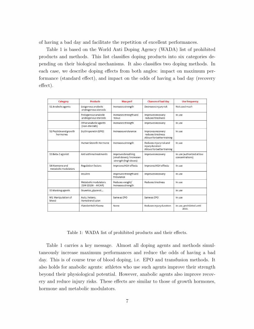
Table 1 is based on the World Anti Doping Agency (WADA) list of prohibited
products and methods. This list classifies doping products into six categories de-
pending on their biological mechanisms. It also classifies two doping methods. In
each case, we describe doping effects from both angles: impact on maximum per-
formance (standard effect), and impact on the odds of having a bad day (recovery
effect).
Table 1: WADA list of prohibited products and their effects.
Table 1 carries a key message. Almost all doping agents and methods simul-
taneously increase maximum performances and reduce the odds of having a bad
day. This is of course true of blood doping, i.e. EPO and transfusion methods. It
also holds for anabolic agents: athletes who use such agents improve their strength
beyond their physiological potential. However, anabolic agents also improve recov-
ery and reduce injury risks. These effects are similar to those of growth hormones,
hormone and metabolic modulators.
7

The recovery effect is usually neglected, as the case of Platelet Rich Plasma
(PRP) illustrates. PRP treatment involves extracting some of the athlete’s blood
and enriching it with platelets, a source of human growth factors. The blood is then
reinjected into the athlete’s body, and this blood manipulation helps the athlete
recover faster from a muscle injury. Up to 2010, the side effects of such treatment
on athletes’ performances were unknown and WADA consequently banned the use of
PRP. However, since 2010 medical studies have shown that PRP has no effect on the
maximum potential performance of an athlete, leading WADA to authorize its use.
The fact that PRP can also be used to decrease risk of injury and injury duration was
not taken into account. But it is unambiguous that reducing risk of injury amounts
to reducing the athlete’s chances of having a bad day. WADA’s position on PRP
shows how institutions focus mainly on how drugs affect maximum performance,
underestimating regularity of performance as a potential target for drug users. We
argue herein that this common view of doping is misleading.
2 Recovery doping: theory
There are two players who compete for a price, the value of which is normalized to 1.
Each player i is characterized by a pair of possible performance levels (ai, ai), with
ai < ai. When in a good state, player i achieves the performance level ai. When in
a bad state he only achieves ai.
Doping is a continuous variable with values between 0 (no doping) and 1 (max-
imal doping). It comes at marginal cost c, and player i exerting doping effort di
has two effects: (i) it increases the higher performance level ai by a quantity a(di),
where a(.) is a non-decreasing function (we denote by ai(di) the quantity ai+a(di));
(ii) it enhances the probability of being in a good state by a quantity h(di): without
doping, each player’s probability of being in a good state is 1/2. With doping, player
i has a probability of 1/2 + h(di) of being in a good state. The function h satisfies
the following assumption:
Hypothesis 2.1 h is a continuous function on [0, 1], C2 on ]0, 1] such that:
(i) h is strictly increasing on [0, 1], h(0) = 0, h(1) = 1/2
(ii) we have h′(1) = 0 and limd→0+ h′(d) = +∞.
8

(iii) h is strictly concave on ]0, 1] and h′′(1) < 0.
Let ai be the performance level realized by player i. Note that Player i wins 1
whenever ai > a−i (where −i denotes the opponent of player i). In case ai = a−i,
the players share the price and obtain 1/2. Player i’s expected payoff is
Ui(di, d−i) = Pr(ai > a−i) +1
2Pr(ai = a−i)− c.di, (1)
where Pr denotes the probability distribution induced by the action profile (di, d−i).
2.1 The standard framework
The purpose of this sub-section is to analyze the standard case where doping only
affects the level of the player’s best performance. The uninterested reader can skip
this part and go directly to the next sub-section. For the moment, let us assume
that there is no recovery effect, i.e. h ≡ 0. Thus doping only increases the maximum
performance of each player. Several models can be examined, from the simplest to
the most elaborate:
(a) homogeneous players (a1 = a2 and a1 = a2) and two doping levels, di ∈ {0, 1}
(b) homogeneous players (a1 = a2 and a1 = a2) and finite doping levels, di ∈{0, d1, . . . , dk}
(c) heterogeneous players (a1 > a2 and a1 > a2) and finite doping levels
(d) heterogeneous players and continuous doping levels di ∈ [0, 1].
We informally discuss all these models here, but Appendix A formalizes and
analyzes each of them. In all these models, the Nash equilibrium, whether in pure
or in mixed strategies, is unique: players do not dope when the doping cost is too
high; both players choose a positive doping level with positive probability otherwise.
This allows us to analyze welfare: we call welfare of player i his payoff at equilibrium
U∗i .
All the models have significantly distinct features. In (a) the resulting 2 × 2
game is a classical prisoner dilemma and the unique Nash equilibrium is in pure
strategies where players dope. In (b) the game exhibits the same characteristics, the
equilibrium is unique and symmetric, and the equilibrium doping level decreases
9

when the cost of doping increases. This model is in line with standard views on
doping. Berentsen (2002) shows that considering heterogeneity in players’ type
introduces drastic changes in the analysis. This is confirmed by model (c), where
the only equilibrium is in mixed strategies, probabilities of doping are asymmetric,
and the marginal cost of doping has asymmetric effects on the different players:
as the cost increases, doping effort decreases for the top dog while it increases for
the underdog. Finally, and more in line with our general model, when doping is a
continuous variable as in (d), the unique Nash equilibrium is in mixed strategies and
decreases for both players (in the sense of first-order stochastic dominance) when
the cost of doping increases.
However, all these models have in common the following crucial features:
Proposition 1 (Heuristics on the standard framework) For the models de-
scribed above:
• Relative to a world without doping, welfare is lower for the underdog (U∗2 ≤U2(0, 0)) and strictly lower for the top dog (U∗1 < U1(0, 0))
• The top dog’s winning probability is lower than in a world without doping.
All proofs are in the Appendix. The standard framework predicts that all ath-
letes fare better when the cost of doping is so high that none would ever dope.
Furthermore, doping increases competition uncertainty. Both features are no longer
true once the recovery effect is taken into account.
2.2 The recovery effect
With doping, the probabilities are changed as follows:
Pr(ai = ai(di)) =1
2+ h(di)
Pr(ai = ai) =1
2− h(di)
Assume, without loss of generality, that a2 < a1 < a2 < a1. The payoff for player 1
is: 12
+ h(d1) + (12− h(d1))(
12− h(d2))− c.d1 if a1(d1) > a2(d2)
12(12
+ h(d1))(12
+ h(d2)) + (12− h(d2))− c.d1 if a1(d1) = a2(d2)
12− h(d2)− c.d1 if a1(d1) < a2(d2)
10

Consider for instance the first equation. If player 1’s maximum performance,
after doping, is higher than that of player 2, then player 1 will win whenever he
realizes his best performance (this happens with probability 1/2 + h(d1)), and will
win when he performs badly (with probability 1/2−h(d1)) only if his opponent also
performs badly (with probability 1/2− h(d2)). Interpretation is similar for the two
other cases.
We show that only two things can happen: first, there can be no equilibrium
to the game when players are very similar to one another in terms of maximum
performance without doping. In that case, because the game is a winner-takes-all
game, there is an arms race to reap all the benefits. As player 2 increases his doping
level, player 1 increases his, until the point where it becomes too costly for player 2
to increase his doping level any more. He then goes back to a no-doping strategy,
and as a consequence player 1 also goes back to the no-doping strategy. The arms
race starts all over again.
Second, if there is an equilibrium (or several equilibria), it is also an equilibrium
of the game in which function a ≡ 0, i.e. a game in which we consider that doping
has no effect on the maximum performance of players.
Lemma 1 Any equilibrium (d∗1, d∗2) of the doping game must be such that a1(d
∗1) >
a2(d∗2).
This lemma implies that if an equilibrium exists, the best player without doping
will still be the best with doping. This allows us to state the following:
Proposition 2 Any Nash equilibrium (d∗1, d∗2) of the doping game is also an equi-
librium of the game with a ≡ 0.
Once the recovery effect is introduced, it alone determines the characteristics
of the equilibrium of the game, regardless of the existence of the standard effect.
Increased maximum performance only determines whether there is an equilibrium or
not. Therefore, focusing on the standard effect leads to partial (no equilibrium) or
non-valid conclusions (when there is an equilibrium). We now turn to the interesting
case: analyzing the game with a ≡ 0 for all d and examining the effects of h(.) on
athletes’ behavior.
11

2.3 Main results
We assume that a ≡ 0 and h satisfies Hypothesis 2.1. For player 1, strategic
interaction arises because he only loses when he is in the bad state and player 2 is
in the good state. If player 2 dopes more, his probability of being in the good state
rises. This in turn raises player 1’s marginal return from doping. Things are very
different for player 2. He loses whenever player 1 is in the good state. Thus doping
efforts are wasted when player 1 makes sufficiently strong efforts.
Given the zero-sum game nature of athletic contests, players’ doping always
reduces the welfare of their opponents. However, it also affects the marginal re-
turn from their opponents’ actions. Call Bri the best response map of player i:
Bri(d−i) := ArgmaxdiUi(di, d−i). A Nash equilibrium is a fixed point of the map
Br := (Br1, Br2).
Proposition 3 (Properties of doping efforts at equilibrium) For any doping
cost c > 0, we have that
(i) Player 1’s best response function increases with player 2’s doping effort, whereas
player 2’s best-response function decreases with player 1’s doping effort. As a
consequence, there is a unique Nash equilibrium d∗ = (d∗1, d∗2).
(ii) The top dog dopes more, i.e. 1 > d∗1 ≥ d∗2 > 0.
Part (i).— The doping effort d2 acts as a strategic complement for player 1,
while d1 acts as a substitute for player 2. The complementarity effect is in line
with the prisoner’s dilemma analysis. The substitution effect is one central piece of
the model because it makes it different from a prisoner’s dilemma and induces the
interesting properties below.
Part (ii).— The top dog is sure to win when he achieves the highest performance
level, which is not true for the underdog. Consequently, the return from doping is
greater for the top dog. This conclusion departs from the standard view on doping.
Proposition 4 (Welfare at equilibrium) We have the following
(i) The underdog fares better in a world without doping: U2(d∗1, d∗2) < U2(0, 0);
(ii) However, when c is not too large, U1(d∗1, d∗2) > U1(0, 0).
12

Doping carries a negative externality, generally at a cost to players. However, if
the cost is not too high (i.e. the authorities are not very repressive), the top dog
benefits greatly from doping. He achieves her best performance more frequently,
and therefore is more likely to win than without doping.
The fact that the best player’s utility is greater with doping than without, added
to the observation that d∗1 > d∗2, explains why it is difficult to fight against doping
and enhance the popularity of a sport at the same time. There might be collusion
between organizers (federations) and the best players, who need one another for
their respective objectives.
Proposition 4 also explains why the best players do not want to fight against
doping. They dope more than the others, and they are actually happy to do their
job in an environment where doping is possible. In contrast, the underdog is hurt
by the doping system: his chances of winning go down and there are doping costs
to pay.
Proposition 5 (Doping effort variations with respect to cost) We have the
following
(i) limc→0+ d∗1 = 1 and limc→0+ d
∗2 = 0;
(ii) The top dog’s doping effort decreases with the cost of doping, that is d(d∗1)/dc <
0;
(iii) The underdog’s doping increases with the cost of doping for low costs, that is
d(d∗2)/dc > 0 for c low enough.
Part (i).— When the cost of doping becomes very low, there are two effects.
First, because doping becomes more attractive, both athletes wish to dope more.
Second, the top dog becomes almost unbeatable because he dopes a lot, so by the
substitution effect, doping becomes less attractive for the underdog. At the limit,
the second effect overrides the first effect.
This result runs counter the argument whereby free access to doping would
lead to a level playing field, because everyone would dope and the results of the
competition would not be affected. Our result suggests the reverse, i.e. the best
athletes might dope at maximum level, whereas the others would not even try.
Competition results would be highly predictable, and absolute performances would
be very heterogeneous.
13

Parts (ii) and (iii).— The cost of doping has an ambiguous impact on the un-
derdog’s equilibrium doping effort. However, we know that his doping effort is
increasing for low costs. This is due to the strategic substituability discussed above:
as the top dog dopes less, the return from doping increases for the underdog.
In the same vein, one can show that targeted tests involve strong redistribution
effects between players. Targeting the best player reduces his doping investment.
Because of strategic substitutability, this also increases the doping investment of
the lower-ranking player, who now has a chance of winning. Thus, overall doping
is ambiguously affected and competitions become more uncertain. Targeting the
underdog decreases doping for both athletes, now due to strategic complementarity.
The underdog is less threatening, which allows the top dog to reduce doping.
2.4 Extension to n players
Our benchmark model with two players contains the main messages. Because we
wish to test our predictions on data, we must account for the fact that competitions
in professional sports take place between more than two players, and check whether
our main predictions still hold. Assume that there are n players, with a1 > a2 >
... > an > a1 > a2 > ... > an. The prize structure is defined through positive real
numbers yn = 0 ≤ yn−1 ≤ ... ≤ y2 ≤ y1 = 1. We assume that the prize structure
satisfies the following convexity condition: for any 1 < j < n,
yj ≤1
2(yj−1 + yj+1)
Proposition 6 We have the following:
(i) As in the two-player case, there always exists a Nash equilibrium. However,
when n ≥ 3, uniqueness does not generally hold
(ii) Any Nash equilibrium d∗ is such that d∗1 > d∗2 > ... > d∗n
(iii) For c small enough, at any Nash equilibrium d∗, U1(d∗) > U1(0) and Un(d∗) <
Un(0).
(iv) Assume k prizes are equal to 0 and the first prize with positive value is yn−k.
Then, given ε > 0, there exists c0 such that, for any c < c0 and any equilibrium
d∗, we have d∗i > 1−ε for all i = 1, ..., n−k and d∗j < ε for all j = n−k+1, ..., n.
14
Part (i) guarantees the existence of a Nash equilibrium, but shows that multi-
plicity can arise from the model. This is due to the fact that the doping effort of any
player is a strategic complement of the doping effort of worse players and a strategic
substitute of the doping effort of better players. This cannot arise in the two-player
case, where the top dog only has a worse player against him, whereas the underdog
only competes against a better player. Multiplicity shows that our model is rich
enough to describe complex phenomena, however points (ii) to (iv) show this does
not create a problem as long as the cost of doping is low, which is the assumption
we make in the next section.
Part (ii), (iii) and (iv) confirm the predictions of the two-player model: better
players dope more than worse players, and they benefit from doping (at least the
best player does; usually, however, there will be a group of top players who will
benefit from doping), while worse players suffer from it. Also, better players tend
to dope at maximum, while the worse players tend to abandon doping when the
cost is low. This is explained by the following: player 1, by doping at maximum,
secures the first position and the highest prize. As a direct consequence, the others
behave as if the first player and the first prize did not exist. For them, the game is
now a competition with n− 1 players and n− 1 prizes. Player 2 is the best player
of this competition, and he secures the highest prize (y2) by doping at maximum.
This goes on as long as there is a positive prize to win, but once all these prizes are
distributed to the best players, the rest no longer have any incentive to dope.
3 Recovery doping: evidence
The last of the predictions delivered by our model is empirically testable: when the
cost of doping tends to zero, performance uncertainty should go to zero and rankings
should be almost deterministic, while an increase in the cost of doping should imply
an increase in performance uncertainty and rankings should be more noisy. This is
what we test in this section.
We provide evidence from a particular sport, cross-country skiing (CCS), and
a particular doping technology, synthetic EPO. CCS is chosen for the following
reasons: though some of the races are short and involve anaerobic skills, CCS is an
endurance sport and therefore particularly exposed to recovery doping. Moreover,
there have been a number of doping scandals, and medical studies provide evidence
of blood manipulation in the 1990s and 2000s. Finally, point attribution is based
15

on individual ranking in the different races. The tournament structure is obvious,
and top athletes have clear incentive to compete at their best level in each race.
We focus on the CCS World Cup, a yearly competition based on 10 to 25 races.
We examine the yearly race-specific rankings between 1987 and 2006 and show
that, in line with our theory, rankings were relatively noisy before EPO was intro-
duced, then became almost deterministic in the 1990s when the use of EPO was
widespread, becoming noisier again after measures against EPO were introduced.
We also document an increase in noisiness in the late 1990s-early 2000s, right after
the introduction of upper limits on hemoglobin concentration ([Hb]).
3.1 Data and methodology
The CCS World Cup is organized by the Federation Internationale de Ski (FIS).
Skiers receive points based on their ranking and the final ranking is obtained by
adding the points collected in each race. We use FIS data on individual rankings in
different races and compute for every year how race-specific rankings are correlated
with the final ranking. More specifically, we calculate Spearman’s rank correlation
between every race of a given year and the final ranking that year. For each race
in the sample we obtain a race-specific correlation, and we average all race-specific
correlations for a given year to compute the yearly correlation. Then we match
changes in yearly correlation with changes in anti-doping environment, by controlling
for potential biases due to changes in the sport itself.
Figure 1 presents the changes in the anti-doping environment, as well as major
events related to the CCS World Cup. Data are not available before 1987 and the
sport was organized differently after 2006 with the creation of super races lasting
several days like the Tour de Ski. These changes preclude any yearly comparison,
so we restrict our attention to the period 1987-2006.
As in cycling, EPO was made available to CCS athletes in the late 1980s. No
tests existed. Given the huge effects on endurance athletes’ performances, EPO was
widely used in the 1990s. Videman et al (2000) document the change in blood profiles
observed for CCS athletes, from 1987 to 1999. The profiles show a large increase in
mean [Hb] from 1989 to 1996. In the 1996-1997 season, an upper bound was imposed
on [Hb], and the threshold became tighter the following season. Correspondingly,
Videman et al (ibid) show a decline in max [Hb]. However, mean [Hb] continued to
increase until 1999.
16

Figure 1: Chronology of changes in CCS events and in the doping environment.
17

Between 1997 and 2001, the anti-doping environment was characterized by un-
certainty. A urine EPO test had been around for years, but it was not efficient. A
test for a plasma expander and EPO-masking agent, hydroxyethyl starch or HES,
became available in 2001, but athletes were not aware of this. At the 2001 Lahti
World Championships, several top skiers in the Finnish team tested positive. In
2002, a test for Darbepoetin Alfa led to the disqualification of Larisa Lazutina and
Olga Danilova of Russia and Johann Muhlegg of Spain from their final races in the
Winter Olympic Games. Blood profiling was introduced in 2002, together with out-
of-competition tests. After that, doping became much more costly. Morkeberg et al
(2009) examine CCS athletes’ blood profiles between 2001 and 2007 and report an
overall decline in [Hb] compared with the 1990s. However, more recent years saw a
change in blood manipulations, i.e. skiers seem to be turning back to transfusions
instead of EPO injection.
There is also evidence of the extent of blood manipulation being heavily cor-
related with performance. Stray-Gundersen et al (2003) analyze blood samples
collected at the 2001 World Championships. They show that “of the skiers tested
and finishing within the top 50 places in the competitions, 17% had ”highly ab-
normal” hematologic profiles, 19% had ”abnormal” values, and 64% were normal.
Fifty percent of medal winners and 33% of those finishing from 4th to 10th place
had highly abnormal hematologic profiles. In contrast, only 3% of skiers finishing
from 41st to 50th place had highly abnormal values.”
Our interpretation of the facts is that doping costs dramatically and uniformly
decreased in the late 1980s-early 1990s, remaining low up to 1997. From 1997 to
2002, it became more hazardous to use EPO and the cost of doping increased. The
uncertainty about EPO and EPO-masking agent detection led a number of athletes
to under-estimate the cost of doping in the early 2000s, leading to the doping scan-
dals of the 2001 World Championships and 2002 Olympics. After 2002, the cost of
doping dramatically increased with certainty.
The FIS rules underwent two major changes over the sample period. Up to
1991, only the top 15 skiers received points in a given race; the dataset reports
their rankings, but not the rankings of those finishing after the 15th position. After
1991, the top 30 skiers received points, and the dataset records the rankings of all
participants. To harmonize years, we only consider the top 15 skiers in each race.
This also allows us to focus on top-level skiers and escape the high volatility in
18

Figure 2: Number of distance and sprint races over time, 1987-2006
rankings generated by including poorly-ranked athletes. Thus, in what follows we
will focus either on the top 15 skiers or on the top 10 skiers.
The second change was brought about by the introduction of sprint races in 1996.
These races are shorter and thus involve different types of skills. The rankings in
such races are by nature less correlated to the final ranking. Figure 2 depicts the
evolution in the number of distance and sprint races. This may create a potential
bias, as 1996 is also the first year where an upper limit on [Hb] was imposed. To
account for that change, we replicate all our correlation computations considering
only distance races. We then reconstruct a hypothetical final ranking where only
points from distance races are counted and we compare race-specific rankings to
that modified final ranking. Removing sprint races from the sample leaves between
10 and 17 races each year, with an average of 13.
Finally, the composition of the group of athletes competing changes from one
race to the other. Skiers do not participate in all races, and self-selection leads to
changes in the proportion of the top 10 or top 15 skiers competing in each race. If
the self-selection pattern varies over time, a resulting potential bias could affect the
yearly volatility of race-specific rankings. To avoid such a bias, we therefore only
19

Figure 3: Test statistics as a function of the minimum number of top-15 skiers, 1987-2006
include races where a sufficiently large number of top skiers participate.
To interpret the yearly correlations, we compute p-values of the nullity test.
While statistical tests exist for the Spearman correlation, they do not exist for
averages of Spearman correlations, so we constructed, by numerical simulations,
the distribution of such averages. The following corresponding p-values are to be
interpreted as the probability that the ranks obtained by top level athletes are
random.
3.2 Results
We start with FIS top 15 skiers and consider all races, including sprint races. The
number of races varies from one year to the next, and the number of top 15 skiers
varies from one race to the next. We only consider races in which at least N (from
4 to 7) of the top 15 skiers participated. A lower N would mean too much variation
across years in the number of top skiers considered, while a higher N would severely
limit the number of races considered per year. Figure 3 displays the value of the
test statistics for every year of the sample. The higher the value, the higher the
correlation between race-specific rankings and yearly final rankings. Figure 4 reports
the corresponding p-values of the null assumption whereby there is no correlation
between the individual race-specific rankings and the overall ranking.
The four curves send the same message: the patterns of the test statistics and of
20

Figure 4: P-values of the zero-correlation test as a function of the minimum number oftop-15 skiers, 1987-2006
the p-values are consistent with the doping pattern previously outlined. The p-values
are relatively high in the early stages of the sample, plummet in 1989 and remain
very close to 0 during the 1990s, in particular in the mid-1990s. Note also that the
change in rules on point attribution does not appear to affect the different curves.
The sudden increase in 2000 and subsequent decline in 2001 and 2002 coincide with
the uncertainty in the anti-doping environment and the 2001 World Championship
and 2002 Olympics doping scandals. The increase after 2002 coincides with the
introduction of blood profiling.
To take account of the introduction of sprint races in the second half of the
1990s, we now report similar computations based on distance races alone and the
associated yearly distance rankings. Being in the top 15 distance skiers does not
carry the same weight as being in the top 15 skiers, sprint races included. The
less well-ranked skiers may not worry much about their final ranking and could
therefore liable to dope. To avoid this bias, Figure 5 focuses on a smaller group of
top athletes, those in the top 10 distance skiers, and confirms the general pattern
shown by Figure 4. Race-specific rankings are more correlated to the final ranking
in the 1990s than in any other period.
3.3 Robustness
The hierarchy among top skiers was remarkably stable during the 1990s, a period of
EPO availability. The fact that p-values decrease with the appearance of EPO and
21

Figure 5: P-values of the zero-correlation test as a function of the minimum number oftop-10 skiers, distance races only, 1987-2006
increase with the introduction of blood tests supports our theory. We now discuss
four potential weaknesses of our approach.
First, the pool of athletes changes over time. In particular, the entry of new skiers
and the exit of older ones may affect pool composition. Irrespective of doping, the
new athletes may perform more or less consistently than the others. This could
affect the relevance of our computations, especially if the timing of such changes
coincides with the overall doping pattern explained above.
The entry of new athletes is unlikely to play a key role, because they do not aim
for the top positions. The proportion of newcomers in the top 15 of the final ranking
was about 6.5% in 1988 and 1989, and zero in the rest of the sample. Similarly, the
proportion of newcomers in the top 10 was zero for the whole sample.
The exit of older skiers is negligible between 1987 and 2006 except for 1998 and
1999, when four of the top ten skiers exited the rankings. Two out of these four
skiers belonged to the top 3, one exiting in 1998 and the other in 1999. These two
athletes were actually big stars, with a very long career and top positions in the
CCS World Cup throughout the 1990s. The emergence of such skiers is a direct
implication of our theory. According to our model, a fall in the cost of doping, such
as experienced in the late 1980s, favors the best athletes. They choose a higher level
of doping and as a consequence the underdogs lower theirs. The probability of top
dog wining a competition increases greatly, consistent with what is observed here.
However, there is an alternative explanation. These athletes could be genetic freaks
who naturally achieve excellent performances. Because these genetic freaks might
22

Figure 6: Test statistics as a function of the minimum number of top-10 skiers, withoutexiters, distance races only, 1988-2006
have contributed to the stability of rankings in the 1990s, we need a robustness check
for our empirical analysis. How can we distinguish between the impact of stars and
a general decline in the cost of doping? The tournament literature that we discuss
in Section 1.1 has already examined the impact of stars on other players’ efforts.
It argues that the presence of such stars is detrimental to the others’ performances
through effort reduction. Thus, if ranking stability in the 1990s was only due to
such stars, then the other players’ rankings should have been very volatile.
To test this argument, we remove the four top 10 skiers who retired in 1998
and 1999 from the dataset. We then reconstruct the hypothetical rankings of each
race as well as the yearly rankings. Finally we carry out the same computations as
before. Figure 6 shows that removing the superstars from the dataset does not alter
our conclusions. Namely, rankings become remarkably stable in the early 1990s,
and correlations fall in 2000 and remain low in the 2000s. This implies that the
remarkable stability of rankings in the 1990s is not due to the presence of the two
superstars.
The second issue with the change of group composition is that our test statistics
compare different skiers across different races. To address this issue, for each year
we follow several specific competitors and see what happens each time they compete
with each other. We consider two groups: a top group composed of the best athletes
in the final distance ranking, and a lower-ranking group. We then form pairs of
athletes by picking one skier from each group. We form as many pairs as possible
and count how many times the competitor from the top group ranks better than
23

Figure 7: Probability of athletes from the top group ranking better than athletes from theweaker group in a given race, 1987-2006
the competitor from the weaker group.
Figure 7 provides our results for three different athletes grouping. In the first
one, we only consider athletes in the top 10. The top group is composed of the top
3, whereas the weaker group is composed of athletes ranked between 5 and 10. We
choose to avoid the number 4 so as to ensure a gap between the two groups. In the
second grouping, we oppose athletes in the top 4 to athletes ranked between 10 and
20. The third grouping opposes the top 5 to athletes ranked between 15 and 50.
The three curves confirm the general pattern previously identified. The proba-
bility of athletes from the top group winning is higher in the 1990s than in the rest
of the sample, there is a sharp decline in the late 1990s-2000, immediately followed
by a spike in 2002, and a steadier decline thereafter.
Third, changes in the organization of the sport design might have altered ath-
letes’ training methods. The emergence of sprint races might have induced athletes
to stop specializing. When first introduced, sprint races represented a tiny share
of all races, and top athletes did not need to perform well in them. In the 2000s,
however, they represented a third of races on average. Rational athletes seeking
points for the final ranking now needed to train for both sprint and distance races.
Top athletes being more all-round, they might have suffered as a result of less con-
sistent results in distance races. On the contrary, a glance at the most successful
race winners in the 2000s shows clear specialization3. Petter Northug from Norway
3See the Wikipedia page http://en.wikipedia.org/wiki/FIS Cross-Country World Cup
24

is actually the only skier who managed to win a significant number of races in both
the sprint and the distance categories. One such athlete is not enough to impact
our results.
Fourth, the overall distance ranking is based on race-specific results. If the
number of distance races changes over time, then the correlation between race-
specific rankings and the overall ranking changes accordingly. As Figure 2 shows,
the number of distance races increases over time. However, the increase occurred
between 1989 and 1996, the period when race-specific rankings became less volatile.
Thus the bias, if any, tends to weaken the pattern discussed here.
3.4 Discussion
Our arguments apply to any contest with player heterogeneity. Once there is a
cheating technology that increases the probability of being in a good state, our
conclusions hold: the best players have more incentives to use the technology, and
as a consequence the gap between best players and weaker players widens.
Cycling.—Contrary to CCS, cycling is a team sport where tactical skills are im-
portant. Moreover, individual ranking in each stage of a multi-stage event is not
relevant: what matters is the final time gap between athletes and their direct oppo-
nents. Candelon and Dupuy (2014) looked at within-team performance inequality
in the Tour de France (TdF). They measured riders’ skills by their speed during the
prologue – an individual short-distance time trial. They show that the final average
speed gap between the leader and each of his teammates increases over time, control-
ling for skill differential. They argue that this reflects the increasing concentration
of TdF monetary rewards on the winner. Our theory provides a complementary in-
terpretation. During the same years, EPO was very popular. Leaders had stronger
incentive to dope than their teammates. They became able to maintain the same
performance level throughout the TdF. When the results of the different stages were
combined, the average speed gap between leaders and teammates increased.
Finance.—Mutual funds compete for capital. Investors allocate their money
across funds according to the past performances of each fund. The managers’ pay is
indexed on their funds’ performance, so managers can be seen as athletes competing
for the highest return. However, managers differ in skills. The ability to provide
a lower volatility at a given mean is an attractive feature of a fund. Fraudulent
accounting is one cheating technology that allows managers to reduce the volatility
25
of their performances: temporary losses can be hidden, thereby smoothing the return
trajectory of the fund. However, it is illegal because of the risk of bankruptcy.
Fraudulent accounting is of greater benefit to the best managers, who can count on
their superior ability to deliver better returns at some future date, so as to restore
the genuine profitability of the fund.
Academic world.—Scientists compete to publish in the most prestigious journals.
Although better researchers have smarter ideas there is some uncertainty about
whether an idea will be confirmed or rejected by proper empirical analysis. In other
words, there is uncertainty about whether an idea is in a good or bad state. There
is a random component here: the history of science is full of beautiful ideas with
no empirical support. Here again, there is a cheating method that increases the
probability of the idea being in a good state: modifying the data to achieve a better
fit with theory. The return on such unethical behavior is actually larger for the best
researchers because they have better ideas, and empirical validation of these good
ideas makes very strong papers.
4 Conclusion
This paper studies the incentive to cheat in contest-like situations. It focuses on
recovery doping, a generic term characterizing cheating technologies that tend to
concentrate performances towards the best individual-specific outcomes. Recovery
doping has heterogenous effects across agents. We argue that the introduction of
such a technology benefits the most talented agents. They become more likely to
win, and performance inequality rises. We develop these arguments in a two-player
zero-sum game with player heterogeneity and performance uncertainty. Cheating
efforts are complementary for the stronger contender, and substitutable for the
weaker one. We then examine a specific contest, the cross-country skiing World
Cup, and a specific cheating technology, synthetic EPO. Race-specific rankings were
more correlated to the final ranking in the EPO era, the 1990s, than in the 2000s.
Thus results were more consistent across races when the cost of doping was low,
becoming more volatile as the cost of doping increased.
26

References
Apesteguia, J., Palacios-Huerta, I., 2010. Psychological Pressure in Competi-
tive Environments: Evidence from a Randomized Natural Experiment. American
Economic Review 100, 2548-2564.
Bhaskar, V., 2009. Rational Adversaries? Evidence from Randomized Trials in
One Day Cricket. Economic Journal 119, 1-23.
Berentsen, A., 2002. The Economics of Doping. European Journal of Political
Economy 18, 109-127.
Berentsen, A., Lengwiler, Y., 2004. Fraudulent Accounting and Other Doping
Games. Journal of Institutional and Theoretical Economics 160, 402-415.
Berentsen, A., Bruegger, E., Loertscher, S., 2008. On Cheating, Doping and
Whistleblowing. European Journal of Political Economy 24, 415-436.
Bird and Wagner, 1997. Sport as a Common Property Resource: A solution to
the dilemmas of doping. Journal of Conflict Resolution 41, 749-766.
Candelon, B., Dupuy, A., 2014. Hierarchical organization and performance in-
equality: evidence from professional cycling. International Economic Review (forth-
coming)
Chiappori, P.-A., Levitt, S., Groseclose, T., 2002. Testing Mixed-strategy Equi-
libria when Players are Heterogeneous: The Case of Penalty Kicks in Soccer. Amer-
ican Economic Review 92, 1138-1151.
Curry, P.A., Mongrain, S., 2009. Deterrence in Rank-Order Tournaments. Re-
view of Law and Economics 5, 723-740.
Eber, N., Thepot, J., 1999. Doping in Sport and Competition Design. Recherches
Economiques de Louvain 65, 435-446.
Glisdorf, K, Sukhatme, V., 2008. Tournament Incentives and Match Outcomes
in Women’s Professional Tennis. Applied Economics 40, 2405-2412.
Klaassen, F.J.G.M., Magnus, J.R., 2009. The Efficiency of Top Agents: An
Analysis through Service Strategy in Tennis. Journal of Econometrics 148, 72-85.
Krakel, M., 2007. Doping and cheating in contest-like situations. European
Journal of Political Economy 23, 988-1006.
Lazear, P.E., Rosen, S., 1981. Rank-Order Tournaments as Optimum Labor
Contracts. Journal of Political Economy 89, 841-864.
Malueg, D.A., Yates, A.J., 2010. Testing Contest Theory: Evidence from Best-
27
of-Three Tennis Matches. Review of Economics and Statistics 92, 689-692.
Morkeberg, J., Saltin, B., Belhage, B., Damsgaard, R., 2009. Blood profiles in
elite cross-country skiers: a 6-year follow-up. Scandinavian Journal of Medicine and
Science in Sports 19, 198-205
Rosen, S., 1986. Prizes and Incentives in Elimination Tournaments. Ameri-
can Economic Review 76, 701-15. Stray-Gundersen, J., Videman, T., Penttila, I.,
Lereim, I., 2003. Abnormal hematologic profiles in elite cross-country skiers: blood
doping or not? Clinical Journal of Sport Medicine 13, 132-137
Sunde, U., 2009. Heterogeneity and Performance in Tournaments: a Test for
Incentive Effects Using Professional Tennis Data. Applied Economics 41, 3199-3208.
Videman, T., Lereim, I., Hemmingsson, P., Turner, M.S., Rousseau-Bianchi,
M.P., Jenoure, P., Raas, E., Schonhuber, H., Rusko, H., Stray-Gundersen, J., 2000.
Changes in hemoglobin values in elite cross-country skiers from 1987-1999. Scandi-
navian Journal of Medicine and Science in Sports. 2000 10, 98-102
Walker, M., Wooders, J., 2001. Minimax Play at Wimbledon. American Eco-
nomic Review 91, 1521-1538.
28

Appendix A - For Online Publication
The standard framework (Section 2.1)
Proposition 1 follows from Propositions 7, 8 and 9 presented below.
• Models (a) and (b)
Two identical players face a binary choice d = 0 or d = 1. The game is summarized
by the following payoff matrix
0 1
0 12, 12
38, 58− c
1 58− c, 3
812− c, 1
2− c
Payoffs in the diagonal cells are obvious. When one player dopes and the other
does not, the doped player wins whenever he performs well (with prob. 12), and he
gets half the prize when both he and his opponent are in a bad state (with prob.12× 1
2). He also bears the cost of doping. This is a a typical prisoner’s dilemma
situation.
Proposition 7 (Homogeneous players)
(i) This game has a unique equilibrium: (0, 0) if c > 1/8 and (1, 1) if c < 1/8
(ii) If both players dope, the winning probabilities are the same as those without
doping
(iii) Ui(1, 1) < Ui(0, 0)
Notice that this easily extends when several doping levels are allowed, i.e. d ∈{0, d1, ..., dk}. Whatever the value of c, there is always a unique and symmetric
equilibrium. Further, any symmetric doping strategy can be an equilibrium for an
appropriate value of c. As the cost increases, the equilibrium level of doping de-
creases. When players use the same doping strategy, the winning probabilities are
unchanged. As a consequence for both players, Ui(d∗, d∗) < Ui(0, 0) for every equi-
librium d∗ > 0.
• Model (c)
29

Two heterogeneous players face discrete doping possibilities. We assume a1 > a2
and a1 > a2, and a(1) > a1− a2. With player 1 standing for the top dog and player
2 for the underdog, the payment matrix is:
0 d
0 34, 14
12, 12− c
d 34− c, 1
434− c, 1
4− c
Proposition 8 (Player heterogeneity) Let a1 > a2, a1 > a2, and a(1) > a1−a2.We have
(i) If c > 1/4, then the only pure-strategy equilibrium is d∗1 = d∗2 = 0;
(ii) If c ≤ 1/4, then there is a unique mixed-strategy equilibrium (γ∗1 , γ∗2), where
γi ∈ [0, 1] stands for the probability that player i plays the doping strategy. It
is such that
– γ∗1 = 1− 4c and γ∗2 = 4c;
– U1(γ∗1 , γ
∗2) = 3/4− c < U1(0, 0) = 3/4 and U2(γ
∗1 , γ
∗2) = 1/4 = U2(0, 0).
By elimination of strictly dominant strategies, (0, 0) is the unique pure-strategy
equilibrium if and only if c > 1/4. Otherwise, there is no pure-strategy equilibrium.
The argument is simple: the underdog may choose to fill the natural performance
gap by using PEDs. If this is profitable for him, then the other player will choose
to dope as a response to the increase in his opponent’s maximum performance. An
arms race then takes place until the disadvantaged player stops doping, because the
quantity of PEDs required has become too high. The best player will respond by
quitting doping too, and as they return to the (0, 0) situation, the arms race starts
all over again.
• Model (d)
Doping is a continuous variable and players are heterogeneous.
Proposition 9 (Continuous doping efforts) Assume that a(d) = d and call δ :=
a1 − a2. Then
(i) If 4cδ ≥ 1, (0, 0) is the only Nash equilibrium and the equilibrium payoff is
(3/4, 1/4);
30

(ii) if 4cδ < 1 there is a unique mixed Nash equilibrium (µ∗1, µ∗2), where the proba-
bility distributions µ∗1 and µ∗2 are given by
µ∗1(0) = 4cδ, µ∗1(]0, d1]) = 4cd1, ∀d1 ∈]0,1
4c− δ];
µ∗2(0) = 4cδ, µ∗2(]δ, d2]) = 4c(d2 − δ), ∀d2 ∈]δ,1
4c].4
and the equilibrium payoff is (1/2 + cδ, 1/4).
The unique pure strategy equilibrium occurs when either the cost is too high
or when the differences in maximum performance levels are too great. In all other
cases, there is no pure strategy equilibrium, for the same reasons as above (arms
race)5. However, there is a unique mixed strategy equilibrium, in which the top dog
has a lower payoff than in a world without doping.
Proof. Point (i) is obvious. We focus on proving (ii). We call Supp(µ) the support
of µ, i.e.
Supp(µ) := {d ∈ R+ : µ(]d− ε, d+ ε[) > 0 ∀ε > 0}
Recall that Supp(µ) is the smallest closed set F such that µ(F ) = 1.
Lemma 2 Let d ≥ 0. Then
d ∈ Supp(µ∗1)⇐⇒ d+ δ ∈ Supp(µ∗2).
Proof. Pick d /∈ Supp(µ∗1) and ε > 0 such that µ∗1(]d− ε, d+ ε[) = 0. Then we claim
that µ∗2(]d+ δ − ε/2, d+ δ + ε/2[) = 0. If this was not the case, then player 2 could
deviate profitably by transferring the weight that µ∗2 puts on ]d+δ− ε/2, d+δ+ ε/2[
onto {d+ δ − ε}. Thus
d /∈ Supp(µ∗1)⇒ d+ δ /∈ Supp(µ∗2).4In other words, µ∗1 and µ∗2 are the sum of a dirac distribution in 0 and a uniform distribution.5The threshold difference in maximum performances, when player 1 is better than player 2, is
given by a((4c)−1). Indeed, the highest possible doping level for player 2 is d such that 5/8− cd >3/8 so d < (4c)−1. When a1(0)−a2(0) > a((4c)−1) then (0, 0) is the unique equilibrium, otherwisethere is no equilibrium.
31

A reverse argument in the previous step gives
d+ δ /∈ Supp(µ∗2)⇒ d /∈ Supp(µ∗1). �
Lemma 3 We have
µ∗1(d1) > 0⇒ d1 = 0; µ∗2(d2) > 0⇒ d2 = 0.
Proof. First we show the following:
Let d1 be such that µ∗1(d1) > 0. Then
∃ε > 0 : ]d1 + δ − ε, d1 + δ[⊂ (Supp(µ∗2))c.
Similarly, let d2 > δ be such that µ∗2(d2) > 0. Then
∃ε > 0 : ]d2 − δ − ε, d2 − δ[⊂ (Supp(µ∗1))c.
Assume that µ∗1(d1) > 0 and, for any ε > 0, there exists d(ε) ∈ ]d1 + δ − ε, d1 +
δ[∩ Supp(µ∗2). Since µ∗1(d1) > 0 there exists ε small enough so that deviating from
d1 + δ − ε to d1 + δ guarantees a strictly higher6 payoff to player 2. The second
statement can be shown with similar arguments.
Now, assume that d1 > 0 is such that µ∗1(d1) > 0. Then, there exists ε > 0 such
that µ∗2(]d1 + δ − ε, d1 + δ[) = 0. Consequently, player 1 can deviate profitably by
transferring the weight that µ∗1 puts on d1 to d1 − ε/2.
For player 2, the same argument states that, for any d2 > δ, we have µ∗2(d2) = 0.
Clearly, we have µ∗2(]0, δ[) = 0. Consequently we just need to prove that µ∗2(δ) = 0.
Assume that µ∗2(δ) > 0. If µ∗1(0) > 0 then player 2 can obtain a strictly better
payoff by transferring the weight on δ to δ + ε. If µ∗1(0) = 0 then player 2 can
deviate profitably by transferring the weight on δ to 0. �
Lemma 4 We have Supp(µ∗1) = [0, b1] and µ∗1(0) > 0. Also we have Supp(µ∗2) =
{0} ∪ [δ, b1 + δ].
Proof. First, we show that if [a1, b1] is the smallest closed interval that contains
Supp(µ∗1), then [a1, b1] = Supp(µ∗1). Similarly, if [a2, b2] is the smallest closed interval
that contains Supp(µ∗2) \ {0}, then [a2, b2] = Supp(µ∗2) \ {0}.6deviating from d(ε) to d1 + δ costs her (at most) εc, but she increases her payoff by a positive
quantity, which is independent of ε.
32

Since Supp(µ∗1) is closed, we have a1, b1 ∈ Supp(µ∗1). Assume that there exists
c1 ∈]a1, b1[ such that c1 /∈ Supp(µ∗1). Then c1+δ /∈ Supp(µ∗2). Now call c1 := inf{d >c1 : d ∈ Supp(µ∗1)}, (resp. c1 := sup{d < c1 : d ∈ Supp(µ∗1)}. By a basic property
of a Nash equilibrium, player 1 must be indifferent between c1 and c1, against µ∗2.
However, by lemma 2, we have µ∗2(]c1 + δ, c1 + δ[) = 0. Hence player 1 has a strictly
higher payoff when he plays c1 than when he plays c1, a contradiction. Exactly the
same argument proves the assertion concerning player 2.
We also know, by lemma 2, that a2 = a1 + δ and b2 = b1 + δ.
Now, assume that µ∗1(a1) = 0. Then we have U2(µ∗1, 0) > U2(µ
∗1, a1 + δ), and
a1+δ ∈ Supp(µ∗2), which is a contradiction to the fact that µ∗ is a Nash equilibrium.
Consequently, a1 = 0 and µ∗1(a1) > 0.7 This proves that Supp(µ∗1) = [0, b1] and
µ∗1(0) > 0. Also we have Supp(µ∗2) = {0} ∪ [δ, b1 + δ]. �
We are now ready to prove the proposition. First, notice that, since U1(0, µ∗2) =
U1(b1, µ∗2), we have
3
4µ∗2(0) +
1
2(1− µ∗2(0)) = 3/4− cb1;
Hence 14(1− µ∗2(0)) = cb1
On the other hand, limε→0+ U2(µ∗1, δ + ε) = U2(µ
∗1, b1 + δ)8, i.e.
−cδ +1
2µ∗1(0) +
1
4(1− µ∗1(0)) = −c(b1 + δ) +
1
2,
which gives cb1 = 14(1−µ∗1(0)). As a consequence, we have µ∗2(0) = µ∗1(0) > 0. Since
U2(µ∗1, 0) = 1
4, we necessarily have −c(δ + b1) + 1/2 = 1/4, i.e. b1 = 1
4c− δ and
µ∗1(0) = µ∗2(0) = 4cδ.
To see why the distributions µ∗1 and µ∗2 are uniform respectively on ]0, b1] and
[δ, b1 + δ], note that, for player 2, we must have U2(µ∗1, 0) = U2(µ
∗1, d2) for any
d2 ∈]δ, b1 + δ]. Hence1
4=
1
4+
1
4µ∗1([0, d2 − δ])− cd2,
which means that µ∗1(]0, d2−δ]) = 4c(d2−δ), for any d2 ∈]δ, b1+δ] and µ∗1 is uniform
on ]0, b1]. Analogously, µ∗2 is uniform on [δ, b1 + δ].
7Recall that 0 is the only point µ∗1 can put a positive weight on.8Note that here we need to take the limit because the payoff function of player 2 is discontinuous
in δ when player 1 plays µ∗1.
33

It is clear that no deviation is profitable for any player as, by construction of µ∗,
we have
U1(d1, µ∗2) = cδ +
1
2, ∀d1 ∈ [0, b1]; U1(d1, µ
∗2) =
3
4− cd1 <
1
2+ cδ, ∀d1 > b1.
Also
U2(µ∗1, d2) =
1
4, ∀d2 ∈ {0}∪ ]δ, d1 + δ]; U2(µ
∗1, d2) = 1/2− cd2 < 1/4, ∀d2 > b1 + δ.
The proof is complete. �
34

Appendix B - Results of the general model
Proof of Lemma 1. Assume (d∗1, d∗2) is a Nash equilibrium such that a1(d
∗1) =
a2(d∗2). Then
limε→0+
U1(d∗1 + ε, d2) > U1(d
∗1, d2),
a contradiction.
Next, if (d∗1, d∗2) is a Nash equilibrium such that a1(d
∗1) < a2(d
∗2) then necessarily
d∗1 = 0. Indeed,
U1(d∗1, d∗2) =
1
2− h(d∗2)− c.d∗1
which can only be sustained as an equilibrium if d∗1 = 0 This implies d∗2 = Argmax U2(0, ·)where
U2(0, d2) =1
2+ h(d2)− c.d2
so that d∗2 = (h′)−1(c). Furthermore d∗2 is such that a2(d∗2) > a1(0), i.e. d∗2 >
a−1(a1 − a2).Also
U2(0, d∗2) > U2(0, 0)
so that 12
+ h(d∗2) > c.d∗2 + 14
We want to show that this cannot be an equilibrium. Assume player 2 chooses
d∗2 and player 1 chooses d∗2 as well. Then a1(d∗2) > a2(d
∗2) and
U1(d∗2, d∗2)− U1(0, d
∗2) =
(1
2+ h(d∗2)
)(1
2+ h(d∗2)
)− c.d∗2
Using 14
+ h(d∗2) > c.d∗2 we have
U1(d∗2, d∗2)− U1(0, d
∗2) >
(1
2+ h(d∗2)
)(1
2+ h(d∗2)
)−(
1
4+ h(d∗2)
)= (h(d∗2))
2 > 0
�
Proof of Proposition 2. Call Vi the payoff functions in the game with a(·) 6= 0
and Ui the payoffs in the game with a(·) = 0. Player 1 is better off in the game with
a(·) = 0: U1(d1, d2) ≥ V1(d1, d2) and conversely for player 2: U2(d1, d2) ≤ V2(d1, d2).
Moreover, if a1(d1) > a2(d2) then Ui(d1, d2) = Vi(d1, d2).
Let d∗ = (d∗1, d∗2) be a Nash equilibrium in the game with a(·) 6= 0. By lemma 1,
35

a1(d∗1) > a2(d
∗2) hence Ui(d
∗1, d∗2) = Vi(d
∗1, d∗2). Consequently, for any d2,
U2(d∗1, d∗2) = V2(d
∗1, d∗2) ≥ V2(d
∗1, d2) ≥ U2(d
∗1, d2),
which means that d∗2 is a best response of player 2 against d∗1 in the game with
a(·) = 0.
On the other hand, d∗1 is a best response of player 1 against d∗2 in the game with
a(·) 6= 0. Let d1 := Br1(d∗2), the best response of player 1 against d∗2 in the game
with a(·) = 0. We have d1 > d∗2 (best responses of player 1 are always greater than
best responses of player 2; see the proof of point (ii) of Proposition 3 in the next
section). Thus
V1(d1, d∗2) = U1(d1, d
∗2) ≥ U1(d
∗1, d∗2) = V1(d
∗1, d∗2) ≥ V1(d1, d
∗2).
This implies U1(d1, d∗2) = U1(d
∗1, d∗2), and the proof is complete. �
Proof of Proposition 3. The payoff functions are given by
U1(d1, d2) = −cd1 +
(1
2+ h(d1)
)+
(1
2− h(d1)
)(1
2− h(d2)
)and
U2(d1, d2) = −cd2 +
(1
2− h(d1)
)(1
2+ h(d2)
)The map h′ is strictly decreasing from (0, 1] to [0,+∞). Hence the inverse
function (h′)−1 is well defined and strictly decreasing from [0,+∞) to (0, 1].
The best-response function of each player results from the first-order condition:
Br1(d2) = (h′)−1(
c
1/2 + h(d2)
),
and
Br2(d1) = (h′)−1(
c
1/2− h(d1)
).
(i) Existence follows from Brouwer Theorem and the fact that Br := (Br1, Br2)
is continuous and maps [0, 1]2 to itself. Uniqueness follows from the fact that Br1
is increasing in d2 and Br2 is decreasing in d1, since (h′)−1 is decreasing.
36

(ii) For any d1, d2,
h′−1(
c
(1/2 + h(d2))
)≥ h′−1
(c
(1/2− h(d1))
),
which means that Br1(d2) ≥ Br2(d1), ∀d1, d2. In particular, d∗1 ≥ d∗2. �
Proof of Proposition 4. Point (i) is a trivial consequence of
U2(d∗1, d∗2) ≤
1
4− cd∗2 = U2(0, 0)− cd∗2.
Next,
∆1(c) := U1(d∗1, d∗2)− U1(0, 0) = −cd∗1 +
1
2(h(d∗1)− h(d∗2)) + h(d∗1)h(d∗2)
Because limc→0+ d∗1 = 1 and limc→0+ d
∗2 = 0 (see Proposition 5). Hence,
limc→0
∆1(c) = 1/4 > 0,
which proves (ii). �
Proof of Proposition 5. Notice that, for any c > 0, (d∗1, d∗2) is the unique so-
lution of the system {h′(d1)(1/2 + h(d2))− c = 0
h′(d2)(1/2− h(d1))− c = 0
where in fact (d∗1, d∗2) ≡ (d∗1(c), d
∗2(c)).
(i) The first limit is a straightforward consequence of the form of the best response
maps. For the second limit, we have, for any c > 0,
h′(d∗2) =c
1/2− h(d∗1)
By concavity of h, we have
1
2− h(d∗1) ≤ h′(d∗1) (1− d∗1) =
c(1− d∗1))1/2 + h(d∗2)
≤ 2c(1− d∗1).
37

Thus we obtain
h′(d∗2) ≥1
2(1− d∗1)→c→0+ +∞,
which implies that
limc→0+
d∗2 = 0.
(ii) and (iii): Using the implicit function theorem, for c > 0,
d(d∗1)
dc=
1
J
(h′′(d∗2)
(1
2− h(d∗1)
)− h′(d∗1)h′(d∗2)
),
andd(d∗2)
dc=
1
J
(h′′(d∗1)
(1
2+ h(d∗2)
)+ h′(d∗1)h
′(d∗2)
),
where J is positive:
J = h′′(d∗1)h′′(d∗2)
(1
2− h(d∗1)
)(1
2+ h(d∗2)
)+ (h′(d∗2)h
′(d∗1))2.
The numerator in thed(d∗1)
dcis negative, which proves (ii).
As for d∗2, we can write its derivative as follows:
d(d∗2)(c)
dc=
1
D
(h′′(d∗1)
(1
2− h(d∗1)
)+ (h′(d∗1))
2
),
where D is positive:
D = h′′(d∗1)h′′(d∗2)
(1
2− h(d∗1)
)2
+ (h′(d∗1))3h′(d∗2).
We study the sign of the numerator, as c→ 0+:
h′(d) ∼d→1 h′(1)− h′′(1)(1− d) = −h′′(1)(1− d);
Moreover,
1
2− h(d) ∼d→1 −h′(1)(1− d)− h′′(1)
2(1− d)2 = −h
′′(1)
2(1− d)2
38

Hence
h′′(d)
(1
2− h(d)
)+h′(d)2 ∼d→1 −
h′′(1)2
2(1−d)2+(−h′′(1)(1−d))2 =
h′′(1)2
2(1−d)2.
This proves that there exists some b > 0 such that
d(d∗2)
dc> 0,
for c ∈ (0, b).�
Proof of Proposition 6. If i < j, we denote by N(i, j) the random variable
equal to the number of players among players {i, ..., j} who are in a bad state. Then,
conditioning respectively on the events ”player i is in a good state” and ”player i is
in a bad state”, the payoff of player i can be written as
Ui(d1, ..., dn) =
(1
2+ h(di)
) i−1∑k=0
yi−kP[N(1, i− 1) = k]
+
(1
2− h(di)
) n−i∑l=0
yn−lP[N(i+ 1, n) = l]− cdi
The first order conditions are, for player i,
h′(di)
(i−1∑k=0
yi−kP[N(1, i− 1) = k]−n−i∑l=0
yn−lP[N(i+ 1, n) = l]
)= c,
which we denote by
αi(d)h′(di) = c.
In the sequel, we will often omit the entry d in αi, if there is no ambiguity.
Proof of (i). Let n = 3 and y := y2 < 1/2. We show the following: given c > 0 and
y ∈]0, 1/2[ there exists a function h satisfying assumption 2.1 and 0 < d3 < d3 <
d2 < d2 < d1 < d1 such that
αi(d)h′(di) = αi(d)h′(di) = c ∀i = 1, ..., 3.
39

This implies that d and d are two distinct Nash equilibria.
Let ε > 0. Pick h1, h2, h3 such that 1/4 + ε > h1 > h2 > h3 > 1/4− ε and define
h3 = h3 + ε, h2 = h2− ε2, h1 = h1 + ε3 It is straightforward to check that for ε small
enough we have
a) 1 > h1 > h1 > h2 > h2 > h3 > h3 > 0,
b) (h2 + h3)/2− (1− 2y)h2h3 > (h2 + h3)/2− (1− 2y)h2h3
c) (h1 + h2)/2− (1− 2y)h1h2 < (h1 + h2)/2− (1− 2y)h1h2
Define
α1 = 3/4 + y/2 + (h2 + h3)/2− (1− 2y)h2h3,
α2 = 1/2 + y/2− (1− y)h1 + yh3, α3 = 1/4 + y/2− (h1 + h2)/2 + (1− 2y)h1h2
and the αi analogously.
Clearly 0 < α3 < α3 < α2 < α2 < α1 < α1 < 1. Let d1 > d1 > d2 > d2 > d3 >
d3 > 0 be chosen such that
α3(h3 − h3)
c< d3 − d3 < α3
(h3 − h3)c
α3(h2 − h3)
c< d2 − d3 < α2
(h2 − h3)c
α2(h2 − h2)
c< d2 − d2 < α2
(h2 − h2)c
α2(h1 − h2)
c< d1 − d2 < α1
(h1 − h2)c
α1(h1 − h1)
c< d1 − d1 < α1
(h1 − h1)c
It is always possible and, if ε was picked small enough at the start of the proof, it
can be constructed so that d1 < 1. We now construct our function h. First let h be
such that, for i = 1, ..., 3,
h(di) = hi, h′(di) = c/αi; h(di) = hi, h
′(di) = c/αi,
40

The set of inequalities above implies that h can be extended as a twice differentiable
function, strictly increasing and strictly concave, which means that it satisfies as-
sumption 2.1. �
Proof of (ii). We show the following: Let n > i ≥ 1 and d = (d1, ..., dn) ∈ [0, 1]n.
Then we necessarily have αi(d) > αi+1(d). As an immediate consequence, if d∗ is a
Nash equilibrium then we have d∗1 > d∗2 > ... > d∗n. Note that, conditioning on the
events ”player i is in a good/bad state”, we have
i∑k=0
yi−k+1P[N(1, i) = k] =
(1
2+ h(di)
) i−1∑k=0
yi−k+1P[N(1, i− 1) = k]
+
(1
2− h(di)
) i−1∑k=0
yi−kP[N(1, i− 1) = k]
As a consequence
i−1∑k=0
yi−kP[N(1, i− 1) = k]−i∑
k=0
yi−k+1P[N(1, i) = k]
=
(1
2+ h(di)
) i−1∑k=0
(yi−k − yi−k+1)P[N(1, i− 1) = k]
Analogously, conditioning on the events ”player i+1 is in a good/bad state”, we have
n−i∑l=0
yn−lP[N(i+ 1, n) = l] =
(1
2+ h(di+1)
) n−i−1∑l=0
yn−lP[N(i+ 2, n) = l]
+
(1
2− h(di+1)
) n−i−1∑l=0
yn−l−1P[N(i+ 2, n) = l]
which implies
n−i∑l=0
yn−lP[N(i+ 1, n) = l]−n−i−1∑l=0
yn−lP[N(i+ 2, n) = l]
=
(1
2− h(di+1)
) n−i+1∑l=0
(yn−l−1 − yn−l)P[N(i+ 2, n) = l]
41

Finally, we obtain
αi − αi+1 =
(1
2+ h(di)
) i−1∑k=0
(yi−k − yi−k+1)P[N(1, i− 1) = k] (2)
−(
1
2− h(di+1)
) n−i−1∑l=0
(yn−l−1 − yn−l)P[N(i+ 2, n) = l] (3)
Notice that∑i−1
k=0 P[N(1, i− 1) = k] =∑n−i+1
l=0 P[N(i+ 2, n) = l] = 1. Moreover, by
convexity of the family (yk)k we have
yi−k − yi−k+1 ≥ yn−l−1 − yn−1 ∀ 0 ≤ k ≤ i− 1,∀ 0 ≤ l ≤ n− i− 1,
with equality only for l = n− i− 1 and k = 0. The sum in (2) is a convex combina-
tion of terms of the form yi−k−yi−k+1 multiplied by a real number greater than 1/2,
whereas the sum in (3) is a convex combination of terms of the form yn−l−1 − yn−lmultiplied by a real number smaller than 1/2. Hence we obtain that αi − αi+1 > 0.
�
Proof of (iii). When c is close to 0, d∗1 is close to 1 (see the proof of (iv) below),
thus the payoff of player 1 is close to y1 = 1. When doping does not exist, his payoff
is a convex combination of all prizes y1 to yn, which is trivially smaller than y1.
Conversely for player n. �
Proof of (iv). Assume first that only yn = 0. For i < n it is sufficient to prove
that αi is bounded from below by a positive constant that does not depend on d.
For i < n, we have P[N(i+ 1, n) = n− i] < 1/2. Hence
αi > yi −(
1
2yi+1 +
1
2yi
)=
1
2(yi − yi+1) > 0
42

Now we turn to i = n. We have
αn =n−1∑k=0
yn−kP(N(1, n− 1) = k)
≤n−1∑k=1
P(N(1, n− 1) = k) = 1− P(N(1, n− 1) = 0)
≤ 1−n−1∏i=1
(1− (1/2− h(di)))
≤n−1∑i=1
(1/2− h(di))
≤n−1∑i=1
h′(di)(1− di)
≤n−1∑i=1
c(1− di)αi
We proved that, for any Nash equilibrium (d∗1, d∗2, ..., d
∗n) we have
h′(di) <2c
yi − yi+1
, ∀i = 1, ..., n− 1; h′(dn) ≥ αn−1∑n−1i=1 1− d∗i
This concludes the proof when yn−1 > yn.
Now, assume that yn−1 = yn = 0. For player n − 1, it is as if player n was
not there: if player n − 1 is in a good state, he will beat player n regardless of his
performance; if player n − 1 is in a bad state, he will get 0 whatever happens. As
a result, player n − 1 acts as if he was competing in a race with n − 2 opponents.
Because he is the worst player, d∗n−1 → 0 as the cost goes to zero. This reasoning
trivially generalizes. �
43