1

A remote-sensing based assessment of ecosystem services for Palawan, the Philippines

Lex Jansen

MSc Thesis in Environmental Sciences

April, 2017

Supervised by: prof.dr. Lars Hein Course code: ESA-80435

Environmental Systems Analysis

2

A remote-sensing based assessment of ecosystem services for Palawan, the Philippines

Lex Jansen

MSc Thesis in Environmental Sciences

April, 2017 Supervisor(s): Examiners: 1) prof. dr. Lars Hein (ESA) 1) prof. dr. Lars Hein (ESA) 2) Boris Kooij (SarVision) 1) prof. dr. Rik Leemans (ESA) Disclaimer: This report is produced by a student of Wageningen University as part of his/her MSc programme. It is not an official publication of Wageningen University and Research and the content herein does not represent any formal position or representation by Wageningen University and Research. Copyright © 2016 All rights reserved. No part of this publication may be reproduced or distributed in any form or by any means, without the prior consent of the Environmental Systems Analysis group of Wageningen University and Research.

3

Abstract

The concept of ecosystem services, which are the benefits provided by ecosystems to

humans, has been developed and popularized in recent decades. Human activities currently

increasingly stress ecosystems and its services. The ecosystem services approach holds the

potential for environmental scientists and policy-makers to collaborate to contribute to the

sustainably develop an area. Ecosystem services research thus far has been extensive, but

findings remain case-specific. This thesis aims to apply the ecosystem services approach for

Palawan, the Philippines, by processing and analysing remotely sensed data. First, several

ecosystem services were selected based on their relevance, feasibility to observe from

remotely sensed data and their inclusion in previous research for Palawan. Ecosystem

services related to carbon dynamics, erosion prevention, agricultural potential and nature

tourism are included. Second, to accurately study these services, land-use maps were

produced for Palawan for 2010 and 2016, using Landsat-5 and Sentinel-2 imagery. In

addition, an SRTM Digital Elevation Model (DEM) was acquired, and processed for errors.

Third, ecosystem services were derived by combining this remotely sensed data with

literature review. Findings of the 2016 land-use maps show that: (i) agriculture and fishponds

dominate southern Palawan; (ii) agriculture in northern Palawan remains limited due to

mountainous geography; (iii) mangrove forest is found throughout all of Palawan, and (iv)

closed tropical forest is mainly found in mountainous inland areas. When the land-use maps

from 2010 and 2016 are compared, the following trends emerge: (i) Vegetation cover

(including wooded grassland) has decreased. This conversion of wooded grassland into

annual agriculture occurs in northern Palawan; (ii) Tropical forest cover (excluding wooded

grassland) has decreased as well. This forest is converted into open forest and wooded

grassland; (iii) approximately 24,000 ha. of open forest has changed into closed forest; (iv)

overall, a substantial amount of annual agriculture has been converted into perennial

agriculture. My findings that relate to ecosystem services show that: (i) carbon storage has

increased by 7.8 million tons C, to a total of 129.1 million tons C. This increase is likely

attributed to an increase in closed forest cover and a slight overall decrease in agricultural

land. (ii) Annual carbon sequestration is reduced by 0.1 million tons C, to a total of 4.6

million tons C; (iii) erosion risk as a result of agricultural expansion is especially apparent in

northern Palawan; (iv) options to expand agriculture have largely been exhausted for

southern Palawan, but not yet for northern Palawan, and (v) due to a good preservation of

pristine ecosystems, municipalities in northern Palawan have high potential for nature

tourism.

Keywords: Ecosystem services, Remote Sensing, GIS, geospatial analysis, land-use,

Palawan, Philippines.

4

Table of content

1 Introduction………………………………………………………………………………………………………………….5

1.1 Background……………………………………………………………………………………………………5

1.2 Research aim…………………..…………………………………………………………………………….8

1.3 Research objectives…………………………………………………………………………………….…8

2 Research Context………………………………………………………………………………………………………..10

2.1 Study area……………………………………………………………………………………………………10

2.2 Ecosystem services………………………………………………………………………………………11

2.3 Remote sensing……………………………………………………………………………………………13

3 Methodology and Tools………………………………………………………………………………………………15

3.1 Overview………………………………………………………………………………………………………15

3.2 Data collection through Remote Sensing……………………………………………………..15

3.3 Data processing……………………………………………………………………………………………19

3.4 Land-use mapping (Landsat-5 & Sentinel-2)…………………………………………………22

3.5 Digital Elevation Model (SRTM)…………………………………………………………………...27

3.6 Analysis of ecosystem services………………………………………………………………..…..28

3.7 Land products (MODIS)…………………………………………………………………................33

3.8 Land-use accuracy assessment…………………………………………………………………….33

4 Results…………………………………………………………………………………………………………………………..35

4.1 Land-use: 2010 and 2016…………………………………………………………………………..…35

4.2 Ecosystem services assessment: 2010 and 2016 ………………………………………….39

4.3 Land products: 2000-2014……………………………………………………………………………46

4.4 Land-use accuracy assessment ……………………………………………………………………47

5 Discussion……………………………………………………………………………………………………………….…….48

6 Conclusion & Future Research……………………………………………………………………………............53

7 Bibliography…………………………………………………………………………………………………………………..55

5

1 INTRODUCTION

1.1 Background

In a period of just a few decades, humanity finds itself at a complex trade-off between some

of its most important activities as recent environment trends raise questions about the

extent to which today’s people are living at the expense of future generations (Daily, 1997;

Ervin et al., 2012; Costanza et al., 2014). Human activity nowadays affects most of the

terrestrial biosphere, either directly through processes such as overharvesting and pollution,

or indirectly through for example global emissions (Kerr et al., 2003). In addition, it is an

increasingly more important factor that brings forward degradation of ecosystems (Foley et

al., 2007; Costanza et al., 2014; MA, 2005; Dobson et al., 2006). While environmental change

has been an acknowledged issue worldwide for a long time, traditionally nature-

conservation policies have focussed primarily on the preservation of biodiversity, ranging

from the gene, to the ecosystem level (Brooks et al., 2006). In more recent times, interest

among scholars has been sparked concerning the goods and services from ecological and

economic services that benefit people (Naidoo et al., 2008). For instance policy-makers

evidently recognize that nature-based solutions (e.g. carbon sequestration due to

reforestation) may very well be more cost-effective than technical solutions (Ervin et al.,

2012). Although an increasing amount of information is being collected on the ecological

value of services provided by natural ecosystems, this information still appears scattered

throughout scientific literature and official reports (de Groot et al., 2002). In addition, this

information often is classified differently by authors, diminishing the opportunities to

conduct comparative analysis (de Groot et al., 2002). In past decades however, a strong

surge in the quantification and valuation of ecosystem services has been witnessed (de

Groot et al., 2002). Following half a century of growing awareness, a bridging concept with

natural sciences, and policy-related social sciences emerged as ‘ecosystem services’ (Braat et

al., 2012).

References to the concept of ecosystem services trace back to the mid-1960s (King et al,

1966; Helliwell, 1969). In the 1970s, researchers started to unify functions of ecosystems

that were deemed beneficial to society under the ecosystem services framework. In

following years, the scientific research on this topic expanded, with an increasing number of

studies each year (Pearce, 1993; Daily, 1997). However, the ecosystem services approach

became particularly popular during the 1990s (Costanza et al. 1992) when it was identified

as an effective method of tackling certain global environmental issues (WCED, 1987). Over

the years, the ecosystem services approach became particularly popular in the developing

world, where effective management of ecosystems can result in much-needed economic

revenue (Fisher et al., 2009). By nature, the ecosystem services approach is a very multi-

disciplinary one; the steps involved in turning initial data collection into effective policy

implementation require a high degree of collaboration between scientists and the public

6

(Fisher et al., 2009). While data collection often is concerned with information science, the

approach also draws from economic theories, social research and policy sciences (Fisher et

al., 2009). Over the years, the exact definition of ecosystem services has remained fluid,

changing between scholars on a regular basis. The definition of ecosystem services used in

this thesis is as follows:

‘’Ecosystem services are the contributions of ecosystems to human well-being’’ (TEEB

Foundations, 2010; MA, 2005)

The significance of research within the domain of ecosystem services is emphasized by the

publication of the Millenium Ecosystem Assessment (MA), ‘’a monumental work involving

the work of 1300 scientists’’ (Fisher et al. 2009). The MA report states that by estimating and

accounting for the economic value of ecosystem services, benefits and social costs that

otherwise would have remained hidden, can be revealed. This makes local, national and

international policy-making more feasible (MA, 2005). Furthermore, an elaborated

understanding of these services is essential in combatting the environmental decline (MA,

2005). The MA report (2005) distinguished a total of 24 different ecosystem services,

grouped together in four different categories: provisioning, regulating, supporting and

cultural ecosystem services. (MA, 2005). What makes this framework unique is that it does

not only elaborate on physical products that are directly harvestable from ecosystems (e.g.

timber, rice) but also processes that are intangible yet crucial to securing human well-being

(e.g. carbon sequestration and tourism). Main indicators to analyse these services are

identified by de Groot et al. (2010): (i) state indicators showing services provided by an

ecosystem and numeric data that describes the provisioning amount of these services; and

(ii) performance indicators that assess the maximum sustainable yield for these ecosystem

services. Based on such indicators, a key finding of the MA publication (2005) was that at a

global level, 15 out of 24 ecosystem services are currently in decline. This is expected to have

a long lasting detrimental effect on human welfare (Fisher et al. 2009).

The usefulness and importance of analysing ecosystems in a quantitative and structured way

are acknowledged by Naidoo et al. (2008), who argue for the importance of quantifying the

services provided by ecosystems in a spatial context. However, estimations regarding

ecosystem services remain crude at best in many regions of the world (Naidoo et al., 2006).

To move forward, there is a need for case-specific exploratory assessments in a temporal

dimension (Hein et al., 2006), that can be used to elucidate not only on the geographical

distribution of ecosystem services, but also the developing trends (Naidoo et al., 2006).

Although scientists have been attempting to improve their understanding of the natural

environment, field-based studies alone often aren’t effective at dealing with the large

volumes of data associated with it (Kerr et al., 2003). A variety of ecological applications also

require data from broad spatial extents that can’t be collected through field-based methods

(Kerr et al., 2003). An efficient way of establishing some crucial ecosystem services is the

land-use, which describes the application of an area. Examples of such applications include

7

agriculture, human residence and forestation. Human domination of the biosphere has led

to accelerating changes in land-use changes worldwide, particularly in the developing world

where industrialization and growing population lead to great environmental stresses (Weng,

2001). This human influence on the biosphere subsequently leads to changes in the

composition, structure and functions of ecosystems so that their capability to deliver

services will erode (Vitousek et al., 1997; Kreuter et al., 2001). Land-use is commonly

described in a geospatial context, visualized on maps. These maps are considered to be a

powerful tool; due to ability of monitoring large datasets, and the relative easiness for

interpretation by people reading reports.

However, traditional methods are usually time-consuming, costly and inefficient for

producing such land-use maps. Instead, for these cases the scientific community has

embraced the use of Geo-information systems (GIS)(Bateman et al., 1999; Jensen, 1996). GIS

technology provides a strong foundation for the storage, processing and analysis of digital

data. Particularly, the field of Remote Sensing, which includes satellite and aerial imagery

data, has made remarkable developments in recent years, and has increasingly become

acknowledged as a highly-effective tool in data-poor regions. Remote Sensing provides cost-

effective, multi-temporal and easy-to-obtain data, and turns them into products that can be

easily visualized and communicated to the public (Weng, 2001). Remote sensing

furthermore generates an unique array of environmental measurements, unobtainable

through field-based methods. Although measurement errors in remote sensing usually are

substantial, through a series of steps data can be processed and corrected to produce results

that often can be readily integrated with other field-based data (Kerr et al., 2003). Even

though such steps are often costly and time-demanding, they still regularly prove to be a

more effective method than field-based practices. Being established several decades ago,

the technology involved with Remote Sensing has been developing remarkably in recent

years, due to many technological advances. For instance, improvements in hardware

technology has ensured data can be collected at a much higher spatial resolution, making it

possible to map smaller features such as roads, ditches and individual crops. Improvements

in software have allowed users of this data to also carry out more complex analysis as well as

making such analysis more accessible and easy to use. The use of Remote Sensing systems is

popular not only for current data, but also for the detection of environmental change, as

many suppliers of satellite data provide this data on online platforms in a multi-temporal

dimension. In either case, given the uncertainty pertaining the accuracy, validation of

measurement results remains an important step in remote sensing practices.

The approach of using land-use data for analysing ecosystem services however is difficult.

Analysis of ecosystem services ideally takes place at a regional scale as this is the scale at

which the effect of their services become most noticeable (Kreuter et al., 2001). However,

the large volume of data involved with analysis at this scale means that this analysis will be

relatively time-consuming. In addition, accurately detecting land-use over a large area is

particularly difficult, as the consistency of the results across the entire study area very much

8

depends on factors such as the dates from which satellite imagery originate from, regional

differences in soil that affect land-use signatures, etc. To warrant a high degree of

consistency across an entire area, it’s best if imagery originate from a similar period of data;

preferably from the same date. High-resolution imagery such as QuickBird, IKONOS and

WorldView (<1m resolution) allow for a very detailed analysis of a study area. However, the

limited swath width of these satellites means that the extent of an image is small, and

therefore a large number of images may have to be collected to cover a project area. In

addition, in land-use change often there is no need to map features at a very high detail.

Instead, to preserve quality through the use of imagery from similar dates, satellites such as

Landsat, MODIS and Sentinel are most commonly used in land-use monitoring. Although the

lower spatial resolution (typically >10 meters) means smaller features often get ignored,

they provide very efficient datasets for monitoring larger ones.

1.2 Research Aim

Many academics, particularly in recent years, conducted assessments of ecosystem services

or ecosystem accounting. These studies often either encompass a local, case-specific analysis

that cannot be generalized to other areas, or assess services globally, but in doing so fail to

address services that are important in a local context. For this reason, studies that elaborate

on the ecosystem services in case-specific contexts are continuously needed (MA, 2005).

Since little research is done to assess ecosystem services for the island of Palawan, this

thesis aims to contribute to this. My research will focus to apply GIS and Remote Sensing to

produce lan-use maps, and to derive is likely crucial to local decision0makers, and helps

Palawan’s future conservation planning and sustainable development.

1.3 Research objectives

In order to achieve the research aim, the overarching objective of this thesis is as follow:

To identify and assess the ecosystem services in Palawan with a spatial and temporal

dimension by using remote sensing approaches

To accomplish this objective, specifying several other objectives is necessary. Currently, the

amount of scientific literature on ecosystem services on Palawan is very limited. Therefore,

the first step necessary to take is to provide an ecosystem services map for Palawan. An

effective way to do so in such a data-poor region, is to use remote sensing data which is

readily available and can be used to assess the entire area in a short amount of time and

gives the user the ability to make an assessment in a multi-temporal context. In this case, to

make comparisons with previous findings possible (i.e. the 2014 study on southern Palawan)

a similar aggregation approach must be used. Ayanu et al. (2012) identified two possible

ways to quantify ecosystem services using remotely sensed data: (1) The remotely sensed

radiation signal can serve as an input for statistical regression and radiative transfer models,

and (2) a land-use classification map can be constructed, with land-use types being linked to

9

ecosystem services. As the first method is mostly oriented towards physical processes, it is

to study most of the relevant ecosystem services on Palawan. Therefore, creating a land-use

map is a more appropriate method. The first objective of this thesis is:

(1) To create land-use maps for 2010 and 2016 using remotely sensed data that

provide spatial information on the most important land-use types in a temporal

dimension.

Based on spectral signatures, several operations can be executed to distinguish different

land-use types. For example, vegetation indices, land classification and spectroscopy are

methods that may be part of a spatial analysis of Palawan. Because the island’s main land-

use types include agriculture and forestation (TWG, 2015), the selected remote sensing

method should be geared towards visualizing types on a land-use map. With the use of the

appropriate land-use map, geospatial data can be combined with other data to produce

ecosystem-services maps. This constitutes the second objective of this thesis:

(2) To transform findings from the land-use map into ecosystem services, and quantify

these services.

Classifications of remotely sensed data, such as in land-use maps, rarely is accurate. This is

caused by limited spatial resolutions and atmospheric distortion on-site. To show how

reliable the results produced in this thesis are, the mapping accuracy Is assessed using high-

resolution Google Earth data as a visual reference. All land-use classes from the land-use

map will be assessed, and findings will be displayed in a confusion matrix. This defines the

final objective of this thesis.

(3) ‘’To validate the land-use and ecosystem services maps on the basis of high-

resolution Google Earth data.’’

In the following chapters, steps are made to accomplish the objectives. First, the context of

this research (e.g. Study area, remote sensing methods and ecosystem services approaches)

are outlined. Following up on this, the approach of producing land-use maps, and analysing

ecosystem services from them, are reflected upon. The results for this are shown in the next

chapter, after which the thesis is finalized with a discussion, conclusion and future research

section.

10

2 RESEARCH CONTEXT

2.1 Study Area

This thesis studies the island of Palawan, Philippines (10.00N, 118.50E), which is also a

province situated in the south-west of the Philippines. The surface area of province amounts

to 14,650 km2 and it encompasses more than 1,700 islands. This study focusses solely on the

main island of the province, Palawan Island, where human activity is most prominent (Figure

1). This proportional but narrow island features a mountain range stretching from the south

to the north of the island, with Mount Mantalingajan as the peak at 2,085m. In southern

Palawan, flat areas featuring agriculture and human settlements dominate the coastal

scenery, while northern Palawan shows a more mountainous geography. The Palawan

province consists of 23 municipalities, of which 13 are located on the Palawan Island, as well

as the capital Puerto Princesa, which is a self-governing city.

Figure 1: Study area of Palawan, Philippines

Demography

According to census data, the population of Palawan amounted to approximately 1,1 million

in 2015, with the capital Puerto Princesa featuring a population of 255,000. Due to booming

immigration in the province, Palawan has accumulated strong cultural influences from

several parts of the world, including China, India, the Middle East and other parts of the

Philippines. As an added result, Palawan also reports the highest annual population growth

out of all Filipino provinces (+3.98%/year). Roman Catholicism is the dominant religion on

the island, but many other religions can be found present as well.

11

Economy

The economy in southern Palawan is largely shaped by agricultural, mining activities and

tourism. Historically, forestry also composed an important part of the local economy,

however due to several policy implementations in recent decades logging activities have

largely been outlawed. Main agricultural products include palay, corn and coconut. Main

mining products include nickel, copper, manganese and chromite. Agriculture can be found

in abundance in southern Palawan. Due to the mountainous terrain, northern Palawan

however is less suited for this. Instead, with places such as El Nido, and the world-famous

Sabang underwater caverns, these part of Palawan attracts a high number of tourists during

the dry season which runs from November until April.

2.2 Ecosystem Services

In 2015, the southern Palawan Technical Working Group (TWG), which consisted of national

experts from the Department of Environmental & Natural Resources (DENR) and the

Palawan Council for Sustainable Development (PCSD), conducted an ecosystem accounting

assessment for southern Palawan. In this assessment, several ecosystem services were

quantified for southern Palawan. Based on their report and studies such as Verburg et al.

(2006), Eder (2006) and Phalan et al. (2016), the main ecosystem services on Palawan Island

were identified. These related to carbon dynamics, agriculture, pollution, mining, fish

production and tourism. When including studies from other world regions (Sumarga et al.,

2014; Law et al., 2015; Schröter et al., 2014; Remme et al., 2015; Estoque et al., 2012), an

even larger array of ecosystem services can be identified that may be of interest on Palawan.

However, time encompassing all of these services in this thesis is impossible. Instead, a

selection is made through a Multi-Criteria Analysis (MCA). An MCA is a popular tool in

environmental impact assessments (Janssen, 2001) and is often used to compare various

alternatives when one common denominator to rank them with does not exist. In this case,

for each of the three criteria ecosystem services are graded from 1 to 5, in which 1 makes it

the least desirable, and 5 the most desirable to include. All three criteria are given an equal

weighing. The scores are then added up, leading to a total score ranging from 5 to 15.

Ecosystem services that score higher are considered to be more appropriate to include in the

research. The following criteria were used for this:

Relevance – An almost infinite number of ecosystem services can be identified when looking

at similar studies elsewhere in the world. However, using the (limited) data available on

Palawan, such as from the 2015 TWG report, it is estimated to what degree the inclusion of

an ecosystem service in this research would be relevant. If this relevance for a service is

unknown, a score of 1 is given.

12

Feasibility – Many ecosystem services require on-site research, or additional data that isn’t

obtainable through remote sensing only. Therefore, for each service it is assessed how well it

could be analysed through optical remote sensing and a Digital Elevation Model.

Previous Research - The 2015 TWG report already analysed several ecosystem services in

southern Palawan. To enable cross-comparisons with findings of that report, ecosystem

services that were analysed before are preferred.

Table 1: a Multi-Criteria Analysis for inclusion of ecosystem services in this research

Ecosystem service Relevance Feasibility Previous Research MCA Score

Carbon Dynamics

Carbon Storage 5 5 5 15

Carbon Sequestration 5 4 5 14

Raw Materials

Hunting 1 2 1 4

Mining 3 3 1 7

Freshwater 3 2 1 6

Medicines 1 2 1 4

Regulating Services

Erosion Prevention 4 5 1 9

Pest Control 2 2 1 5

Pollination 2 3 1 6

Landslide control 5 5 1 11

Flood Control 3 3 1 7

Water regime regulation 3 3 1 7

Water purification 4 2 3 9

Waste regulation 1 1 1 3

Storm protection 2 3 1 6

Biodiversity

Species Habitat 4 2 1 7

Patch connectivity 3 4 1 8

Reforestation potential 3 3 1 7

Agriculture

Soil fertility 2 3 1 6

Irrigation 2 3 1 6

Food production 5 5 5 15

Perennial crop production 5 3 5 13

Agricultural suitability 5 5 1 11

Tourism

Trekking 1 2 1 4

Nature Tourism 4 3 1 8

Based on the MCA scores of each ecosystem service, a selection was made for the services

that were preferred to the included in the research. To avoid inclusion of too many

13

ecosystem services that would require too much time to analyse, seven services were

chosen for inclusion (Table 2).

Table 2: ecosystem services included in this research

Carbon Dynamics

Carbon storage

Carbon Sequestration

Regulating Services

Soil erosion prevention

Agriculture

Food production

Perennial crop production

Agricultural suitability

Tourism

Nature Tourism

2.3 Remote Sensing

Given the data-poor characteristics of Palawan and the need for a remote study, applying

satellite remote sensing methods is an especially useful tool to achieve the aim of my

research. Satellite remote sensing is widely used for the estimation of biophysical

parameters of the surface environment (Kerr et al., 2003). Before reflected radiation reaches

a satellite, there are two ‘noise’ effects from the environment that affect it: (i) the surface of

the Earth, which will contain biophysical information that is of interest to the study; and (ii)

the atmosphere (e.g. cloud cover) that may interact with the signal from the Earth’s surface,

or even block it out completely reducing data consistency (Kerr et al. 2003). To deal with

this, several methods to exist to produce accurate results nonetheless.

In this thesis, optical remote sensing is used to produce two land-use maps (2010 and 2016).

Optical remote sensing is a type of remote sensing that relies on wavelengths associated

with the visible light and infrared spectrum. This form of data is preferred as it is regarded as

a very efficient method of distinguishing the general land-use classes that will be used in this

thesis. A great variety of (optical) satellite data however exists. With varying spatial,

temporal and radiometric resolutions, these different satellite data each have their specific

applications. In addition, some satellites are private-owned and therefore the produced data

will have to be paid for. In this thesis, only satellite data that are freely available were

considered.

In 2014, the Philippines National Mapping and Resource Information Authority (NAMRIA)

produced land-use maps for southern Palawan for 2010 and 2014. The findings show that

southern Palawan consists primarily of forests, wooded grasslands and annual and perennial

agriculture, as shown in Table 3.

14

Table 3: land account assessment of the TWG (2015).

Land account Land cover 2010 (ha) Land cover 2014 (ha)

Annual cropland 48,000 50,000

Plantations 114,000 116,000

Closed forest 28,000 33,000

Open forest and

grasslands

334,000 323,000

Mangrove forest 17,000 17,000

Considering the preference for higher-resolution data with a radiometric resolution that

would be suited for distinguishing these classes, Sentinel-2 was identified as the best data

source from which the 2016 land-use map can be derived. As Sentinel-2 was only launched

in July 2015 however, it is unable to provide data for the 2010 land-use map. Instead, for the

2010 land-use map Landsat-5 data will be used. For both land-use maps, the same land-use

classes will be identified so that a trend analysis can be conducted.

Table 4: Main characteristics of the satellites from which the land-use maps will be derived

Sensor Spatial resolution Temporal resolution Since

Landsat-5 30m 16 days 1984

Sentinel-2 10m 10 days 2015

The following chapter elaborates which steps were taken to produce land-use maps from

the original Landsat and Sentinel satellite data. As these steps are largely the same for both

satellite data, the descriptions and examples will be largely focussed on the more recent,

2016 Sentinel-2 data.

15

3 METHODOLOGY AND TOOLS

3.1 Overview

For the land-use mapping of Palawan for 2010 and 2016, ERDAS IMAGINE 9.1 is used for the

software. This software is specifically made for the analysis of remotely sensed data, and

comes with a vast supply of operations. The main operations used in this research include

supervised and unsupervised land classification, clump & sieve, filters and the ERDAS spatial

modeller. For the assessment of ecosystem services, as well as producing the corresponding

maps, ArcGIS 10.3 is used.

Satellite images of Sentinel-2 are used for the 2016 land-use mapping, obtained from the

Amazon Web Services (AWS) as 110x100km tiles. The Sentinel-2 images originate from 2010

and 2016, and are at a 10m spatial resolution. Out of the original 13 bands, 6 bands were

preserved as a means of data reduction, keeping the purpose of the study in mind so that

doing this will not undermine the goals. As Sentinel-2 only was launched by the European

Space Agency (ESA) in 2015, for the 2010 land-use mapping Landsat-5 imagery is used

instead, at a 30m spatial resolution. The same bands as Sentinel-2 were preserved for the

Landsat-5 data, to maintain consistency as much as possible between the results. Finally, for

the land products, MODIS data was acquired for every year, from 2000 to 2015. This data

comes either at a 250 or 500m spatial resolution and is used as a way to provide further

context to the other findings of the research. Every analytical step and interpretation will be

further described for each relevant subject below.

3.2 Data collection through Remote Sensing

Datasets for both Sentinel-2 and Landsat-5are available at an interval of respectively 10 and

16 days, meaning that for one year, around 25-35 datasets will be available. To select the

most suited datasets for use in this research, two factors were kept In mind:

(1) Image quality: An important factor to take into account when selecting satellite

images is cloud cover, which can render parts of the landscape completely invisible,

either directly or indirectly through cloud shadow. Strictly speaking, there are no

rules regarding cloud cover for which the quality of an image is acceptable or not.

However ideally, agricultural areas that are often small in size (in comparison with

forests) and difficult to extrapolate through filtering should remain visible. Therefore,

in this thesis imagery with low overall cloud cover, particularly in agricultural and

residential areas, will be preferred. In the case there are no cloud-free images for a

certain scene, several images will be collected, and combined to attempt to

eliminate the effect of cloud cover. Although this may come at the expense of quality

of classifications (due to different reflectance values between days) this ultimately

leads to the highest overall quality of the land-use maps.

16

(2) Growing season: in order to ensure that annual agriculture can be captured on an

image, it is necessary to find periods in the year during which these crops are

considering to be in their growing season (Lobell et al., 2013). If not, these areas

most likely will show up simply as barren sites. The main crop types and their annual

growing pattern were identified for Palawan, according to the International Rice

Research Institute (IRRI) and the Philippine Department of Agriculture (DA – PhilRice).

Although there is no one set standard for agricultural practices on Palawan, in

PhilRice found some general and common patterns. Table 5 shows the results of

these findings. Satellite imagery from months that have all crop types at their

growing season peak, will have preference for the land-use map. If no suitable

images can be found for these months, data from other months will be used.

Table 5: Growing season of major crops in the Philippine, and suitability during image

acquisition (Y/N) dates to detect them.

Crop Jan Feb Mar Apr May Jun Jul Aug Sep Oct Nov Dec

Rice Y Y N N N N N Y Y N N Y

Corn Y Y Y/N Y Y Y Y Y/N N Y Y Y

Perennial Y Y Y Y Y Y Y Y Y Y Y Y

Taking the two points into account, table 6 and 7 show the datasets that were acquired for

Landsat-5 and Sentinel-2. To reduce the effect of cloud cover on image quality, the study

area was divided in four (Landsat-5) and seven (Sentinel-2) tiles, for which imagery was

separately collected. Cloud-free imagery from December to February was favoured, and

used as a dominant input. Supplementary imagery was collected from other months of the

year, to replace areas that weren’t visible in the dominant images.

Table 6: Satellite imagery for the 2010 land-use classification (Landsat-5). The dominant is

the primary image used for land-use classifications. However, pixels that are eliminated (e.g.

due to cloud or shadow cover) will be replaced with data from supplementary imagery.

Geographical area Dominant image1 Supplementary images

1 Bataraza, Brooke’s Point,

Rizal, Sofronio Españiola,

Quezon, Narra

19 February, 2010 None

2 Aborlan, Puerto Princesa

City

1 December, 2009 19 February, 2010

3 Roxas, San Vicenze,

Dumaran, Taytay

20 June, 2010 12 February, 2010

4 El Nido 12 February, 2010 None

17

Table 7: Satellite imagery for the 2016 land-use classification (Sentinel-2)

Geographical area Dominant image Supplementary images

1 Bataraza 12 January, 2016 None

2 Brooke’s Point 21 May, 2016 None

3 Rizal 12 January, 2016 None

4 Quezon, Sofronio Española,

Narra

12 January, 2016 None

5 Puerto Princesa City,

Aborland

12 January, 2016 None

6 Roxas, San Vicenze,

Dumaran

8 February, 2016 9 March and 18 May, 2016

7 Taytay, El Nido 11 February, 2016 8 February and 21 May, 2016

Figure 2: Layout of the Landsat-5 and Sentinel-2 tiles for Palawan.

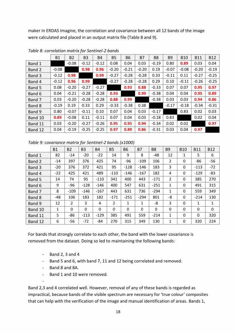
As images are collected for a very large geographical area, without data management file

sizes and computation times will become very significant. For this reason, a Principal

Component Analysis (PCA) is conducted to determine which bands can be left out of the

images. In the PCA, a correlation and covariance matrix is created for one of the images.

With this matrix, correlations between each band can be investigated. If two or more bands

have a very strong correlation (>0.85, Kwarteng et al. 1989), the assumption is that there is

no added benefit of having both bands in an image, and therefore it will suffice to only

include the band with the smallest variance. For the PCA, image number 4 of the Sentinel-2

data was selected, as it features a wide variety of relevant land-use classes. With the Model

18

maker in ERDAS Imagine, the correlation and covariance between all 12 bands of the image

were calculated and placed in an output matrix file (Table 8 and 9).

Table 8: correlation matrix for Sentinel-2 bands

B1 B2 B3 B4 B5 B6 B7 B8 B9 B10 B11 B12

Band 1 -0.08 -0.12 -0.12 0.08 0.04 0.03 -0.19 0.80 0.89 0.03 0.04

Band 2 -0.08 0.98 0.96 -0.20 -0.21 -0.20 0.19 -0.07 -0.08 -0.20 -0.19

Band 3 -0.12 0.98 0.99 -0.27 -0.28 -0.28 0.33 -0.11 0.11 -0.27 -0.25

Band 4 -0.12 0.96 0.99 -0.27 -0.28 -0.28 0.29 0.10 -0.11 -0.26 -0.25

Band 5 0.08 -0.20 -0.27 -0.27 0.93 0.88 -0.33 0.07 0.07 0.95 0.97

Band 6 0.04 -0.21 -0.28 -0.28 0.93 0.99 -0.38 0.04 0.04 0.95 0.89

Band 7 0.03 -0.20 -0.28 -0.28 0.88 0.99 -0.38 0.03 0.03 0.94 0.86

Band 8 -0.19 0.19 0.33 0.29 -0.33 -0.38 0.38 -0.17 -0.18 -0.34 -0.31

Band 9 0.80 -0.07 -0.11 0.10 0.07 0.04 0.03 -0.17 0.83 0.02 0.03

Band 10 0.89 -0.08 0.11 -0.11 0.07 0.04 0.03 -0.18 0.83 0.02 0.04

Band 11 0.03 -0.20 -0.27 -0.26 0.95 0.95 0.94 -0.34 0.02 0.02 0.97

Band 12 0.04 -0.19 -0.25 -0.25 0.97 0.89 0.86 -0.31 0.03 0.04 0.97

Table 9: covariance matrix for Sentinel-2 bands (x1000)

B1 B2 B3 B4 B5 B6 B7 B8 B9 B10 B11 B12

Band 1 82 -14 -20 -22 14 9 8 -48 12 1 5 6

Band 2 -14 397 376 425 74 -96 -109 106 2 0 -86 -56

Band 3 -20 376 372 421 95 -128 -146 183 3 0 -113 -72

Band 4 -22 425 421 489 -110 -146 -167 182 4 0 -129 -83

Band 5 14 74 95 -110 341 400 443 -171 2 0 385 270

Band 6 9 -96 -128 -146 400 547 631 -251 1 0 491 315

Band 7 8 -109 -146 -167 443 631 736 -294 1 0 559 349

Band 8 -48 106 183 182 -171 -251 -294 801 -8 0 -214 130

Band 9 12 2 3 4 2 1 1 -8 3 0 1 1

Band 10 1 0 0 0 0 0 0 0 0 0 0 0

Band 11 5 -86 -113 -129 385 491 559 -214 1 0 0 320

Band 12 6 -56 -72 -84 270 315 349 130 1 0 320 224

For bands that strongly correlate to each other, the band with the lower covariance is

removed from the dataset. Doing so led to maintaining the following bands:

- Band 2, 3 and 4

- Band 5 and 6, with band 7, 11 and 12 being correlated and removed.

- Band 8 and 8A.

- Band 1 and 10 were removed.

-

Band 2,3 and 4 correlated well. However, removal of any of these bands is regarded as

impractical, because bands of the visible spectrum are necessary for ‘true colour’ composites

that can help with the verification of the image and manual identification of areas. Bands 1,

19

9 and 10 were not found to be correlating to the other bands, but were removed regardless

as they hold information on respectively aerosols, water vapour and cirrus clouds which

aren’t relevant for this research.

3.3 Data processing

The Landsat-5 data was already present as a Level-2 product. Imagery contained all relevant

bands with the geometric projection for Palawan (WGS 84 North 50). As a result, limited

data pre-processing steps had to be taken. However, the Amazon Web Service from which

Sentinel-2 data was derived, only supplied data at the Level-1C product level. This data

provided a separate image for each band at the band-specific spatial resolution, with no

geometric projection. To deal with this, bands with a spatial resolution other than 10m (i.e.

the 20m resolution of band 7 and 8a) were converted to a 10m spatial resolution by using a

first order polynomial. For the resampling technique, Nearest Neighbour was used. With all

bands at the same spatial resolution, they were stacked together to compose one image,

and this image was geo-referenced to WGS 84 North 50.

Atmospheric and Bad line Correction

Cloud cover is a very common occurrence in optical satellite imagery, and for the case of

Palawan this was no exception. There are two ways in which atmospheric distortion is

present in optical remote sensing data (Iqbal, 2011): (1) Molecular absorption, and (2)

Scattering effects. Molecular absorption typically contributes very little to atmospheric

distortion (Iqbal, 2011). However, scattering effects does result in a significant altering of

satellite data, making it impossible to accurately map affected areas. These scattering effects

can be divided into three subgroups: (1) Rayleigh Scattering, which results from the scatter-

effect of air (primarily O2 and N2) molecules. (2) Mie Scattering, which is caused by bigger

particles that are present aerosols. (3) Non-selective Scattering, which is the result of

scattering by very large particles (e.g. rain and smoke) and is of minor importance on a clear

day (Iqbal, 2011).

For the dominant imagery from table 6 and 7, a cloud mask file was created to eliminate

pixels affected by atmospheric distortion. To detect such pixels, the following model

functions was used in the ERDAS Spatial Modeller, based on Miettinen et al. (2010):

Equation 1 (Landsat-5): EITHER 0 IF (($n1_bataraza(1)>150) AND ($n1_bataraza(2) >150)

AND ($n1_bataraza(3) >150)) OR 1 OTHERWISE

Equation 2 (Sentinel-2): EITHER 0 IF (($n1_bataraza(1)>2000) AND ($n1_bataraza(2) >2000)

AND ($n1_bataraza(3) >2000)) OR 1 OTHERWISE

20

Pixels that show very high reflectance for all three visible spectrum bands, which in practice

was only shown to correlate with cloud covered areas, will be assigned a value of 0. All other

pixels will be assigned a value of 1. By using the Mask function in ERDAS, pixels with a value

of 0 were then removed from the original image.

Figure 3: The masking of pixels with atmospheric distortion, for the Bataraza area, Palawan

Figure 3 shows this process for the southern tip of Palawan island. Although very small

pockets of atmospherically distorted pixels remain, the vast majority were eliminated. Even

though Sentinel-2 utilizes bands (1 and 10) for the detection of aerosols and cloud cover,

tests with them were found to be less successful than the cloud masking method with the

visible spectrum bands. A possible explanation for this is that while these Sentinel-2 bands

are most suited for detection of cirrus clouds, atmospheric distortion for Palawan was also

caused by other cloud types.

However, although the visible spectrum cloud masking is effective for eliminating cloud

cover areas, it doesn’t deal with areas affected by cloud shadow. Instead, for this purpose an

unsupervised classification was run for all dominant images. In an unsupervised

classification, pixels with a similar spectral pattern are clustered together in classes through

a statistical approach (Ozesmi et al., 2002). Although the scientific world doesn’t provide a

set standard of the number classes in which pixels are divided, studies such as MacLeod et

al. (1998), Kempka et al. (1992) and Bouvet et al., (2003) use several hundreds of classes for

what is called as ‘’extensive cluster busting’’ to separate pixels (Jensen et al., 1987). Palawan

stretches over a vast area, and features a wide variety of land-use types. In order to

accurately map areas distorted by cloud shadow, an unsupervised classification was run with

500 classes, through 6 iterations, a maximum deviation of 0.75 and a maximum convergence

of 0.950. After running the analysis, classes corresponding to cloud shadow were grouped

together, and turned into a mask to further remove atmospheric distortion from the

dominant imagery. Finally, in a few cases bad lines were present on the edge of the satellite

image. These bad lines usually were only a few pixels wide, but nonetheless were manually

removed, and supplemented with valid data.

21

Supplementary imagery

After masking out all cloud cover and cloud shadow pixels from the dominant imagery, they

were merged together with supplementary imagery of the same area, but from a different

date using the Mosaic tool in ERDAS Imagine. Valid pixels in the dominant images were

retained, however the removed pixels were filled up with the data from the supplementary

imagery. Figure 4 shows the result of this for the Roxas, Dumaran, Taytay and San Vicenze

municipalities. Although after merging the images some invalid (black) pixels still remained,

the number of such pixels was significantly reduced and allowed for a more accurate land-

use classification in the affected areas. Image merging was conducted only for dominant

imagery that had significant clouded areas that would affect the land-use classification

result. For instance, although figure 4 shows cloud cover in the Bataraza municipality, these

clouds are concentrated over the more mountainous areas where all land-use most likely

consists of forest vegetation.

Figure 4: Mosaic process results of two images. The left image is the dominant image; the

right image is the dominant image supplemented with the data of another image.

Final map composition

After map compositions are made for all Landsat and Sentinel-tiles, the images are joined

together with the Mosaic tool. By adding a coordinate system and coordinates (for Sentinel-

2) the tiles will perfectly fit together, creating a single image for all of the island. Figure 5

shows the final map results for Landsat-5 and Sentinel-2. Note that colour mismatches

throughout the image are caused by a difference in acquisition dates of imagery, which

however won’t affect land-use classification results.

22

Figure 5: Map compositions of Palawan for 2010 (Landsat-5) and 2016 (Sentinel-2)

3.4 Land-use mapping

To maintain consistency with previous research, as well as retaining the option for cross-

comparisons, the same land-use classes that NAMRIA used for their 2010 and 2014 land-use

mapping, the following classes were mapped in this research:

Definitions: The descriptions below are taken directly from the Forest Resources Assessment

(2005), set up by the Food and Agriculture Organization (FAO) of the United Nations. These

definitions have been used as a guiding line for previous land classifications of Palawan.

Closed and Open forest - Formations where trees in the various storeys and the

undergrowth cover a high proportion(>40 percent) of the ground and do not have a

continuous dense grass layer. They are either managed or unmanaged forests in advanced

state of succession and may have been logged-over one or more times, having kept their

characteristics of forest stands, possibly with modified structure and composition.

Mangrove forest - Forested wetland growing along tidal mudflats and along shallow water

coastal areas extending inland along rivers, streams and their tributaries where the water is

generally brackish and composed mainly of Rhizopora, Bruguiera, Ceriops, Avicenia,

Aegiceras, and Nipa species having more than 40 percent crown cover.

Marshland - Natural land area usually dominated by grass-like plants such as cat tails and

sedges which are rooted in bottom sediments but emerge above the surface of the water. It

contains emergence vegetation and usually develop in zones progressing from terrestrial

habitat to open water.

23

Wooded Grassland - Area predominantly vegetated with grasses, such as Imperata,

Themeda, Saccharum; and where thetrees cover 5 to 10 percent of the area and their height

may reach 5 meters at maturity.

Shrubs - Refer to vegetation types where the dominant woody elements are shrubs i.e.

woody perennial plants, generally of more than 0.5 meter and less than 5 meters in height

on maturity and without a definite crown. The growth habit can be erect, spreading or

prostrate. The height limits for trees and shrubs should be interpreted with flexibility,

particularly the minimum tree and maximum shrub height, which may vary between 5 and 7

meters approximately.

Annual crop land - Land cultivated with crops with a growing cycle under one year, which must be newly sown or planted for further production after harvesting.

Perennial crop land - Land cultivated with long term crops that do not have to be replanted for several years after each harvest; harvesting components are not timber but fruits, latex and other products that don’t significantly harm the growth of the planted trees or shrubs; orchards, vineyards and palm plantations, coffee, tea, sisal, banana, abaca, etc. are included in this category.

Built-up area - Compose of areas of intensive use with much of the land covered by

structures. It includes cities, towns, villages, strip developments along highways,

transportation, power, and communication facilities, and areas occupied by mills, shopping

centres, industrial and commercial complexes, and institutions that may, in some instances,

be isolated from urban areas. The built-up class was further distinguished between roads

and cities for ecosystem services calculations.

Inland water - Area occupied by major rivers, lakes and reservoirs.

Fishpond - Body of water surrounded by land mainly intended for commercial raising of fish

Barren - Land not covered by (semi) natural or artificial cover. This includes among others,

sand dunes, river wash and rocky or stony areas.

Attempts were made to further classify perennial agriculture. Signature collection for

Palawan is difficult due to a lack of ground truth data, and therefore signatures from other

areas of the Philippines were collected. These signatures contained information on a total of

15 perennial classes, including some that are important for Palawan, such as palm oil and

coconut. However, the signatures proved to be too spectrally similar for optical remote

sensing data, and as such land-use classifications with them resulted in a highly fragmented

land-use map that was impossible to interpret. Even after grouping perennial classes that

showed some spectral similarities, such as in figure 6, classifications still remained

impossible. Through comparisons with high-resolution imagery from Google Earth, it was

24

clear almost all sites were getting wrongfully classified, or mixed up with forest vegetation.

Instead, for this research only one perennial class was used.

Further attempts were also made at distinguishing irrigated and rainfed annual agriculture.

This was done through observing the NDVI of both annual growing seasons, as outlined by

Xiao et al. (2005). 250m spatial resolution MODIS-data was retrieved, and for a 16-day

period the NDVI was observed. If significant NDVI differences were present between the two

growing seasons, the agriculture was assumed to be rainfed, as NDVI differences would

emerge as a result of less precipitation in the drier season. The accuracy for this however

remains difficult to analyse.

Figure 6: Spectral profile of three categories of perennial cropland

A first way to separate some of the classes was done through calculating a Normalized

Difference Vegetation Index (NDVI), using the following formula:

Equation 3: (NIR – RED) / (RED + VIS)

NDVI values (ranging from -1 to 1) correlates strongly with vegetation density and

‘greenness’ of a pixel, with higher values being linked to more vegetation. This allows to

easily separate classes such as forests and wooded grasslands, from classes like annual

agriculture, barren sites and roads. In this research, pixels with an NDVI value higher than

0.700 were assumed to be highly likely to contain forest vegetation, and therefore were

separated from pixels with an NDVI of 0.699 and below.

After separating all pixels into two classes, a supervised classification was run for the entire

island. Signatures were collected for each land-use class, from various points on the island. A

minimum signature pixel count of 1000 pixels was used per class, although most signatures

had a considerably higher count. Figure 10 shows examples of signatures that were collected

for each class. Open and Closed forest were initially grouped together, as supervised

classification results proved unsatisfactory in attempts to distinguish them.

25

Figure 10: Example of signatures for each land-use class

Closed/Open forest

Mangrove Forest

Marshland

Wooded Grassland

Shrubs

Fishpond

Inland water

Barren

Built-up

Annual agriculture1

Perennial agriculture

1: In the case of annual crop land, the spectral profile may differ a lot depending on the age

of the crops. Therefore, for this land-use class several sub-classes were initially identified, and

later grouped together again.

26

An issue presented itself with the classification of perennial cropland. Because optically,

matured perennial cropland is so spectrally similar to forests, misclassifications occurred for

many pixels. However, although known perennial crop fields were shown to be classified as a

mixture of perennial and forest, the amount of pixels that were classified as perennial were

much higher than for forest areas. To remove loose forest pixels in perennial fields, the

following formulas were used:

Equation 4: FOCAL DENSITY ( $n1_perennialsupra , $n3_Custom_Float , USE_VALUE 2 ,

APPLY_AT_VALUE 2 )

Followed by:

Equation 5: CONDITIONAL { ($n5_perennialdensity >= 25) 0 , ( $n5_perennialdensity< 25)

1 }

With these formulas, first the density of perennial pixels around a single forest pixel in a

10x10 pixel grid is calculated. If at least 25% of the surrounding pixels are perennial pixels,

the forest pixel would also be classified as one. If this is not the case, nothing will happen.

The end result of this approach is that areas that pixels that were most likely misclassified

inside perennial fields, would be converted to perennial instead.

Table 11 shows the ID roster that was used for the land-use maps. Empty slots were

reserved for different types of perennial crops (14 and 15), but remained unused. After

producing the land-use maps, the Clump tool was used to combine areas of pixels with the

same land-use. Using the Sieve tool, the value of areas smaller than 1 hectare was changed

to the output of a 7x7 Majority function, to remove the ‘’pepper and grain’’ effect of the

images. The resulting image was manually adjusted in some areas (e.g. mangrove forests

being allocated in mountainous areas, due to low reflectance as a result of shadow effects) .

The initial land-use maps had a merged closed and open forest class. The options to separate

this class was investigated through the use of several formulas from literature. Examples of

these formula include:

Equation 6: Advanced Vegetation Index (AVI): (B4 +1) (256 – B3) (B4 – B3)1/3

Equation 7: Shadow Index (SI): Sqrt((256 – B2) (256-B3))

Equation 8: IRECI: (B7-B4)/(B5/B6)

Equation 9: S2REP: B5 + 35 * (((B7 + B4)/2) – B5)/(B6 – B5)

Accurately classifying open and closed forests proved to be very difficult, partly due to the

shadow effect in mountainous areas, and partly due to the lack of satellite data from below

27

the top canopy. Based on results produced with all four formula, S2REP showed the most

consistent patterns and therefore was preferred.

Table 11: ID table of the land-use classes

ID Class

0 Unclassified

1 Water

2 Barren

3 Built-up

4 Fishpond

5 Shrubs

6 Wooded Grassland

7 Open Forest

8 Closed Forest

9 Marshland

10 Mangrove Forest

11 Irrigated Agriculture

12 Rainfed Agriculture

13 Perennial Agriculture

14

15

16 City

3.5 Digital Elevation Model (SRTM)

In order to analyse some of the ecosystem services on Palawan, other factors besides land-

use come into play. One of such factors is the elevation and the slope angle of an area. A

Digital Elevation Model (DEM) can provide such data. For Palawan, the accuracy of different

DEMs, present at a 1 and 3-arcsecond spatial resolution, supplied by ASTER and SRTM3 was

assessed.

Although the ASTER DEM is present in the higher spatial resolution of 1-arcsecond , very

significant errors were present, particularly in vegetated hillside areas. An assumption for

this is that the treeline pattern is too rigid, leading to relief in canopy being mistaken for

actual elevation changes. The SRT3 DEM, at a 3-arcsecond spatial resolution, proved to be

much more accurate and was therefore used in this thesis. For this original elevation data of

this DEM, a first-order derivative was used to derive a slope angle map, which was used later

in this research for the assessment of some ecosystem services.

28

Figure 7: Slope angle maps of ASTER and SRTM-3, derived from a Digital Elevation Model

(both of the same area)

3.6 Analysis of Ecosystem services

This sections outlines the exact steps that are taken to analyse each of the ecosystem

services from table 2.

Carbon Storage and Sequestration

Although directly measuring carbon stock on the basis of remote sensing is not uncommon,

it usually has to be supplemented with additional data for a very accurate analysis. For

instance, studies such as Saatchi et al. (2011), Gomez et al. (2008) and Goetz et al. (2009)

combine optical, microwave and Lidar imagery with field data in order to obtain site-specific

values on carbon stock. This kind of an approach is not possible to achieve for many reasons.

Therefore, instead carbon stock measurements from studies in comparable areas are used,

and combined with the land-use classes from Landsat-5 and Sentinel-2 to approximate the

carbon storage on Palawan.

Table 12: Carbon storage of ecosystem units on Palawan

Ecosystem unit Carbon stock (tons C/ha)

References

Closed forest 184 Davis et al. (1995), Gibbs et al. (2007), Lasco et al. (2003), Ojha et al. (2009), Germer et al. (2007), Liu et al. (2008) Open forest 130

Mangrove forest 1,083 Dung et al. (2016), Donato et al. (2011), Murdiyarso et al. (2015), Kaufmann et al. (2011)

Wooded grassland 32 Liu et al. (2008), Murdiyarso et al. (2015)

Shrubland 15 Adame et al. (2013)

Marshland 723 Xu et al. (2013),Singh et al. (2012), Waddington et al. (1998)

Perennial cropland 32 Sumarga et al. (2014), Xie et al. (2001)

Annual cropland 0 Fang et al. (2007), Li (2002)

29

Table 13: Carbon sequestration of ecosystem units on Palawan

Ecosystem unit Carbon sequestration

(tons C/ha/year)

References

Closed forest 5.4 Brown et al. (1984), Lugo et al. (1992), Birdsey et al. (2006), Andreae et al. (2002), Kendall et al. (2005), Malhi et al.

(1998), Dixon et al. (1994), Mizoguchi et al. (2012), Komiyama et al. (2007)

Open forest 4.5

Mangrove forest 8.5 Zha et al. (2010), Komiyama et al. (2007), Alongi (2014), Bouillon et al. (2008)

Wooded grassland 3.5 Potter et al. (2011), Scott et al. (2014)

Shrubland 3.1 Lal (2004), Scott et al. (2014), Clark et al. (2004),Gilmanov et al. (1996)

Marshland 0.9 Hirano et al. (2007), Hopkinson et al. (2013), Frolking et al. (1998), Waddington et al. (1998)

Annual Agriculture 3.5 Kroodsma et al. (2006), Ceschia et al. (2010), Pan et al. (2004), Zheng et al. (2008), Lu et al. (2013), Shang et al.

(2011), Song et al. (2005)

Perennial cropland 2.5 Sumarga et al. (2014), Germer er al. (2007), Basri et al. (2015), Bhattacharyya et al. (2014)

Soil Erosion prevention

Soil erosion is a major environmental threat to the sustainability and productivity of

agricultural systems (Pimentel et al., 2004). Soil erosion is especially present in steep sloped

areas with a limited amount of vegetation, in which the nutritious top part of this soil is

washed away by precipitation or land and mud slides (Pimentel et al., 2004). Several

methods for assessing the soil erosion in an area exist. The most popular method for this is

the USLE formula, which relies a large number of input data (e.g. soil composition, slope

lengths) to produce an accurate estimation. Unfortunately, this input data is largely

unavailable for Palawan, and therefore the USLE formula can’t be carried out. Instead, based

on this formula, a more simple approach was designed for this research.

Two types of relevant input data exist for Palawan; land-use maps produced by optical

remote sensing analysis, and a slope map derived from the SRTM DEM. For both of these

data, values were grouped into four classes. For the slope steepness, this was done as

follow:

Class A: 0 to 5% slope steepness

Class B: 5 to 15% slope steepness

Class C: 16 to 30% slope steepness

Class D: 31% and higher slope steepness

Next, based on the land-use map, there were also four classes derived based on vegetation

density:

30

Class 1: Very high vegetation – Closed, open and mangrove forest

Class 2: High vegetation – Wooded grassland, marshland

Class 3: Medium vegetation – Shrubs, perennial cropland

Class 4: Low/no vegetation – Annual agriculture, built-up, barren, fishponds

Based on the slope steepness and vegetation class a pixel belongs to, it will be allocated to

one of five groups that show the risk of erosion in that pixel. This methodology is in

accordance with , in Gobena (2003):

Table 14: Soil erosion risk assessment on the basis of slope steepness, and vegetation density

Soil erosion risk Class combination

Very Low A1, A2, B1

Low soil B2, A3, C1, D1

Moderate A4, B3, C2, D2

High C3, B4

Extreme C4,D3, D4

Agricultural Suitability

To assess where agriculture may potentially expand to on Palawan in the future, and

agricultural suitability map is produced. This map is produced on the basis of slope

steepness and proximity to a road network. In 2013, a presidential order was issued in the

Philippines prohibiting the cutting and harvesting of timber in natural forests. This also

applies if the purpose of it is establish agricultural fields. For this reason, in this research it is

assumed that only pixels belonging to the shrubs and wooded grassland classes is at risk of

land conversion.

For the slope steepness, and road proximity factors, three groups relating to the suitability

for agricultural expansion were created. This data was combined to derive one, overarching

suitability map. For the slope steepness this was as follow:

No suitability: 31% and higher slope steepness

Low suitability: 21 to 30% slope steepness

Moderate suitability: 11 to 20% slope steepness

High suitability: 10% and lower slope steepness

For the road proximity, it was assumed that areas far out of reach of a road network (more

than 6km. away) were too inaccessible for farmers to be at a reasonable risk for land

conversion. Usually, for a road to be mapped correctly in Sentinel-2, it had to be at least 5

meters wide. This means very small roads, or ones well covered below forest canopy, may

not have been included.

31

No suitability: 6.1km away and further

Low suitability: 4.1km to 6.0km away

Moderate suitability: 2.1km to 4.0km away

High suitability: 2.0km away and closer

Based on the slope steepness and road proximity class a pixel belongs to, it will be allocated

to one of five groups that show the suitability of agricultural expansion in that pixel.

Table 15: Agricultural suitability assessment on the basis of slope steepness, and proximity to

roads

Overall Suitability Conditions

Very Low L/L

Low L/M, M/L

Moderate M/M, L/H, H/L

High M/H, H/M

Very High H/H

Nature Tourism

To model the nature tourism factor, several factors are taken into account. These include

land-use type, slope steepness, road proximity, city proximity, elevation and proximity to

water. For each factor, a score was given based on how favourable it would be to support

nature tourism. This approach is in agreement with studies such as Dung et al. (2007) and

Pareta (2013). Table 15 shows the exact criteria, and corresponding scores. For the land-use

data, it was assumed more ‘authentic’ areas such as mangrove or closed forests, were more

favoured. For cities and roads, it was assumed that areas located too far away from them

would either be inaccessible, or too time-consuming too visit for a tourist. Multi-ring buffers

were created for these features in ArcGIS 10.3. For the slope steepness, it was assumed a

slope that is too steep isn’t traversable. Finally, for the elevation and hydrology input data,

special scenery (i.e. high-elevated point, or an inland lake) were regarded as special features

that will capture the attention of a tourist. However, these were ‘bonus’ points a pixel could

score, as not meeting these criteria will not result in the pixel being classified as unsuitable

for nature tourism.

Although nature tourism encompasses more than tourists visiting forested areas (e.g. the

world-famous Sabang underwater caverns) the limitations linked to only relying on remote

sensing data have to be taken into account.

32

Table 16: Nature tourism suitability map

Input Data Data Description Score

Land-use Shrubs/Wooded Grassland 1

Open Forest 5

Mangrove/Closed Forest 10

Other Unsuitable

Major Cities Distance < 500m. 1

Distance >500m. but <5km. 5

Distance >5km. but <10km. 3

Distance >10km. but <15km. 1

Distance >15km. Unsuitable

Roads Distance <200m. 1

Distance >200m. but <500m. 5

Distance >500m. but <1km. 3

Distance >1km. but <3km. 1

Distance >3km. Unsuitable

Slope Slope <5° 5

Slope >5° but <10° 3

Slope >10° but <15° 1

Slope >15° Unsuitable

Elevation Elevation <250m. 1

Elevation >250m. but <500m. 3

Elevation >500m. but <750m. 5

Elevation >750m. 7

Hydrology Distance to water <200m. 5

Distance to water >200m. but <500m. 3

Distance to water >500m. 1

By adding up the scores for each input data, an overall nature tourism suitability score is

derived. Depending on the value, this will result in a pixel being assigned to one of the six

suitability classes in table 17. Even though the maximum suitability score is 37, in practice

pixel values came nowhere near this number. Instead, a scoring system was applied that

resulted in a relatively even histogram distribution.

Table 17: Nature tourism suitability ranking

Suitability Overall Score

Not suitable 0

Very low 1-9

Low 10-12

Moderate 13-14

High 15-17

Very high 18+

In principle, all areas with a value of 1 or higher, would be suited for nature tourism as they

met the minimum conditions four different criteria. However, it is assumed that tourists will

33

always favour the best quality in terms of nature experience, making pixels with a higher

overall score especially likely to be linked to nature tourism.

3.7 Land product (MODIS)

As a means of supplementing additional data regarding the vegetation on Palawan, as well

as strengthening my thesis’ final conclusions, two land products were analysed using MODIS

satellite data: GPP and NPP. In both cases, data was collected over a 16-day period for the

first two weeks of January each year, from 2000 to 2014. The values found from these maps

were visually represented on a map and summed up and added in a graph in order to see

ongoing trends. As MODIS has a temporal resolution of 1-2 days, this means that for a 16-

day period several images were compared, with only valid pixel (i.e. no cloud cover) being

selected to compose one final image for that year. In some cases however, invalid pixels still

remain due to persistent cloud cover. If this is the case, these pixels will be removed through

the ERDAS Spatial Modeller.

Using the MOD-17A2 and MOD-17A3 bands, data on the GPP and NPP of Palawan at a 250m

spatial resolution was collected. The GPP and NPP in this case can be seen as important

indicators for the condition of the natural ecosystems, providing a proxy on biomass content

and carbon sequestration. The total GPP and NPP for Palawan will be calculated and

compared for each year. Due to weather patterns (e.g. precipitation) in some years the GPP

and/or NPP may be higher. In order to visually show environmental degradation, values from

2008-2014 and 2000-2007 will be averaged. These two maps will then be compared, and

pixels that show a significant decrease in NPP (more than 10%) will be marked on the map.

It was also attempted to map the Vegetation Continuous Fields (VCF) , using MOD-44B data.

The VCF can provide information on the forest cover, that could be useful for more

accurately mapping some of the natural ecosystems on Palawan. However, analysis of the

data showed that a very considerable number of pixels showed invalid (i.e. value 0) results.

Even after combining data from several years together, large portions of the forested areas

on Palawan remained impossible to analyse. As such, it was decided not to include VCF data

in this thesis.

3.8 Land-use accuracy assessment

Due to limitations in the spatial and radiometric resolutions of the optical satellite data used

to produce the land-use maps, misclassifications may occur. Without analysing the degree to

which this has happened (i.e. what percentage of pixels were classified correctly) it will

remain unknown to what extent the land-use maps actually are accurate and useful. For this

reason, an accuracy assessment will be carried out. Due to time constraints, this assessment

34

will only be carried out for the 2016 land-use map that was produced by using Sentinel-2

data.

For each land-use class on the map, 40 randomly distributed points will be selected in areas

that have high-resolution data available. For each of these points, the coordinates will be

linked to ‘true colour’ satellite data from Google Earth. As 2016 data through Google Earth is

limited, in some cases data from 2013-2015 was selected. Through visually interpreting

these coordinates, it will be determined whether or not the land-use map was accurate. As

visually distinguishing shrubs and wooded grasslands, and open and closed forest, remain

very difficult, these classes will be unified for the accuracy assessment. This will result in the

collection of a total of 320points for Palawan Island.

The results of this assessment will be displayed in a confusion matrix, displayed as table 18.

For each class, the user’s and producer’s accuracy will be measured. In this case, user’s

accuracy refers to fraction of correctly classified pixels with regards to all pixels classified as

this class in the land-use map. The producer’s accuracy is the fraction of correctly classified

pixels with regard to all pixels of that ground truth class. The overall accuracy of the map is

determined by dividing the total number of correctly classified pixels, by the total number of

test pixels.

Table 18: Confusion matrix used for accuracy assessment of the 2016 land-use map

Classified data BA BU FI WG FO MA AA PA Total User’s accuracy

Barren (BA)

Built-up (BU)

Fishpond (FI)

Wooded Grassland (WG)

Open/Closed Forest (FO)

Mangrove forest (MA)

Annual agriculture (AA)

Perennial agriculture (PA)

Producer’s accuracy

Overall accuracy:

35

4 Results

4.1 Land-use: 2010 and 2016

Figure 8: Land cover map of Palawan in 2010

36

Figure 9: Land cover map of Palawan in 2016

37

Table 19: Global Land-use Statistics for Palawan

Land cover Land-use 2010 (ha) Land-use 2016 (ha) Trend

Annual crop 157,830 127,686 -30,144

Perennial crop 74,835 99,254

Fishpond 854 1,945

Wooded Grassland1 271,546 254,394 -17,152

Open Forest 515,954 482,835 -33,119

Closed Forest 87,323 112,087 +24,764

Mangrove2 25,036 31,750 +6,714

1: For 2016, this also includes Shrubs

2: For 2016, this also includes Marshland

Table 20: 2010 Land-use per municipality (ha)

Municipality Agriculture Perennial Fishpond Wooded Grassland

Open Forest

Closed Forest

Mangrove

Aborlan 14,705 6,852 5 11,995 27,541 8,920 1,202

Bataraza 16,908 10,955 63 8,827 3,890 349 6,726

Brooke’s Point 9,967 7,660 10 13,462 18,407 2,305 3

Dumaran 5,781 839 0 11,503 22,321 3,632 920

El Nido 7,928 4,115 0 6,606 34,112 281 789

Narra 27,924 4,459 130 9,207 23,302 2,389 641

Puerto Princesa City 8,517 5,839 0 46,519 113,759 23,293 4,020

Quezon 13,007 10,290 369 37,030 51,267 14,370 1,788

Rizal 10,119 7,584 86 50,210 46,205 3,640 4,218

Roxas 4,173 3,370 0 25,636 43,395 8,009 1,694

San Vicente 5,006 868 0 6,647 56,191 12,891 0

Sofronio Española 14,857 8,625 435 23,446 16,997 2,206 1,442

Taytay 18,510 3,244 0 19,980 58,151 4,766 1,578

Table 21: 2016 Land-use per municipality (ha)

Municipality Agriculture Perennial Fishpond Wooded Grassland

Open Forest

Closed Forest

Mangrove

Aborlan 7,358 4,832 3 17,978 26,743 7,873 1,655

Bataraza 7,999 14,356 47 8,085 6,570 206 6,415

Brooke’s Point 4,932 11,450 6 12,977 19,165 5,110 44

Dumaran 8,092 1,062 0 8,954 19,493 836 1,885

El Nido 7,382 2,486 2 15,300 18,950 5,367 1,881

Narra 20,087 6,707 265 15,314 22,475 2,074 973

Puerto Princesa City 9,740 6,124 391 39,951 104,387 33,047 5,668

Quezon 5,557 11,014 646 32,413 49,661 20,634 2,714

Rizal 8,471 10,971 79 39,562 48,843 9,579 3,191

Roxas 7,514 4,501 17 20,399 51,443 8,350 1,684

San Vicente 6,660 1,447 0 5,342 53,778 11,581 723

Sofronio Española 9,336 20,524 482 17,723 14,647 4,888 981

Taytay 24,416 3,066 4 19,760 45,667 1,906 3,905

38

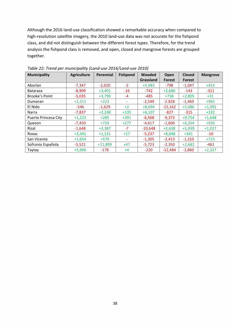
Although the 2016 land-use classification showed a remarkable accuracy when compared to

high-resolution satellite imagery, the 2010 land-use data was not accurate for the fishpond

class, and did not distinguish between the different forest types. Therefore, for the trend

analysis the fishpond class is removed, and open, closed and mangrove forests are grouped

together.

Table 22: Trend per municipality (Land-use 2016/Land-use 2010)

Municipality Agriculture Perennial Fishpond Wooded Grassland

Open Forest

Closed Forest

Mangrove

Aborlan -7,347 -2,020 -2 +5,983 -798 -1,047 +453

Bataraza -8,909 +3,401 -16 -742 +2,680 -143 -311

Brooke’s Point -5,035 +3,790 -4 -485 +758 +2,805 +31

Dumaran +2,311 +223 - -2,549 -2.828 -1,469 +965

El Nido -546 -1,629 +2 +8,694 -15,162 +5,086 +1,092

Narra -7,837 +2,248 +135 +6,107 -827 -315 +332

Puerto Princesa City +1,223 +285 +391 -6,568 -9,372 +9,754 +1,648

Quezon -7,450 +724 +277 -4,617 -1,606 +6,264 +926

Rizal -1,648 +3,387 -7 -10,648 +2,638 +5,939 +1,027

Roxas +3,341 +1,131 +17 -5,237 +8,048 +341 -10

San Vicente +1,654 +579 - -1,305 -2,413 -1,310 +723

Sofronio Española -5,521 +11,899 +47 -5,723 -2,350 +2,682 -461

Taytay +5,906 -178 +4 -220 -12,484 -2,860 +2,327

39

4.2 Ecosystem services assessment: 2010 and 2016 Carbon Storage

Figure 10: Carbon storage in 2010 and 2016, in tons C/ha

Table 23: carbon storage per land-use class

Land cover 2010 Carbon stock (millions tons C)

2016 Carbon stock (millions tons C)

Trend (millions tons C)

Perennial crop 2.39 3.18 +0.79

Wooded Grassland 8.69 8.14 -0.55

Open Forest 67.07 62.77 -4.30

Closed Forest 16.07 20.62 +4.55

Mangrove 27.11 34.39 +7.28

Total 121.33 129.10 +7.77

Table 24: Carbon storage per municipality

Municipality 2010 Carbon stocks 2016 Carbon stocks Trend

Aborlan 7.12 7.44 +0.32

Bataraza 8.49 8.56 +0.07

Brooke’s Point 3.50 4.26 +0.76

Dumaran 4.96 5.05 +0.09

El Nido 5.68 6.06 +0.38

Narra 4.60 5.06 +0.46

Puerto Princesa City 25.10 27.26 +2.16

Quezon 10.83 14.58 +3.75

Rizal 13.09 13.19 +0.10

Roxas 9.89 10.84 +0.95

San Vicente 9.92 10.12 +0.20

Sofronio Española 5.20 5.09 -0.11

Taytay 10.89 11.25 +0.36

40

Carbon Sequestration

Figure 11: Carbon sequestration in 2010 and 2016

Table 25: carbon sequestration per land-use class

Table 26: carbon sequestration per municipality

Land cover 2010 Carbon sequestration (millions tons C/year)

2016 Carbon sequestration (millions tons C/year)

Trend (millions tons C/year)

Annual crop 0.55 0.45 -0.10

Perennial crop 0.19 0.25 +0.06

Wooded Grassland 0.95 0.89 -0.06

Open Forest 2.32 2.17 -0.15

Closed Forest 0.47 0.60 +0.13

Mangrove 0.21 0.27 +0.06

Total 4.69 4.62 -0.07

Municipality 2010 Carbon sequestration

2016 Carbon sequestration

Trend

Aborlan 0.29 0.28 -0.01

Bataraza 0.19 0.18 -0.01

Brooke’s Point 0.20 0.21 +0.01

Dumaran 0.19 0.17 -0.02

El Nido 0.22 0.22 0

Narra 0.26 0.26 0

Puerto Princesa City 0.88 0.89 +0.01

Quezon 0.52 0.52 0

Rizal 0.49 0.49 0

Roxas 0.37 0.40 +0.03

San Vicente 0.37 0.36 -0.01

Sofronio Española 0.26 0.25 -0.01

Taytay 0.44 0.41 -0.03

41

Food production

Figure 12: Food production in 2010 and 2016

Table 27: Food production per municipality

Municipality 2010 Food production (ha)

2016 Food production (ha)

Trend (ha)

Aborlan 14,705 7,358 -7,447

Bataraza 16,908 7,999 -8,909

Brooke’s Point 9,967 4,932 -5,035

Dumaran 5,781 8,092 +2,311

El Nido 7,928 7,382 -546

Narra 27,924 20,087 -7,837

Puerto Princesa City 8,517 9,740 +1,223

Quezon 13,007 5,557 -7,450

Rizal 10,119 8,471 -1,648

Roxas 4,173 7,514 +3,371

San Vicente 5,006 6,660 +1,654

Sofronio Española 14,857 9,336 -5,521

Taytay 18,510 24,416 +5,906

Total 157,830 127,686 -20,144

42

Perennial production

Figure 13: Perennial production in 2010 and2016

Table 28: Perennial production per municipality

Municipality 2010 Perennial production (ha)

2016 Perennial production (ha)

Trend

Aborlan 6,852 4,832 -2,020

Bataraza 10,955 14,356 +3,401

Brooke’s Point 7,660 11,450 +3,790

Dumaran 839 1,062 +223

El Nido 4,115 2,486 -1,629

Narra 4,459 6,707 +2,248

Puerto Princesa City 5,839 6,124 +385

Quezon 10,290 11,014 +724

Rizal 7,584 10,971 +3,387

Roxas 3,370 4,501 +1,131

San Vicente 868 1,447 +579

Sofronio Española 8,625 20,524 +11,899

Taytay 3,244 3,066 -178

Total 74,835 99,254 +24,419

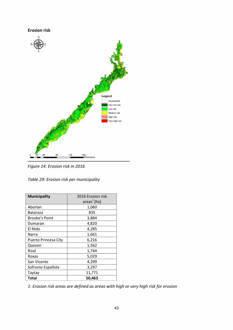
43

Erosion risk

Figure 14: Erosion risk in 2016

Table 29: Erosion risk per municipality

1: Erosion risk areas are defined as areas with high or very high risk for erosion

Municipality 2016 Erosion risk areas1 (ha)

Aborlan 1,060

Bataraza 835

Brooke’s Point 3,884

Dumaran 4,820

El Nido 4,285

Narra 1,661

Puerto Princesa City 6,216

Quezon 1,562

Rizal 1,744

Roxas 5,029

San Vicente 4,299

Sofronio Española 3,297

Taytay 11,771

Total 50,463

44

Agricultural potential

Figure 15: Agricultural potential in 2016

Table 30: Agricultural potential per municipality

Municipality 2016 Agricultural potential

areas1 (ha)

Aborlan 14,419

Bataraza 5,811

Brooke’s Point 2,092

Dumaran 6,986

El Nido 12,699

Narra 8,705

Puerto Princesa City 28,184

Quezon 22,601

Rizal 32,757

Roxas 15,415

San Vicente 4,695

Sofronio Española 11,663

Taytay 16,261

Total 182,288

1: Agricultural potential areas are defined as areas with high or very high potential for

agriculture

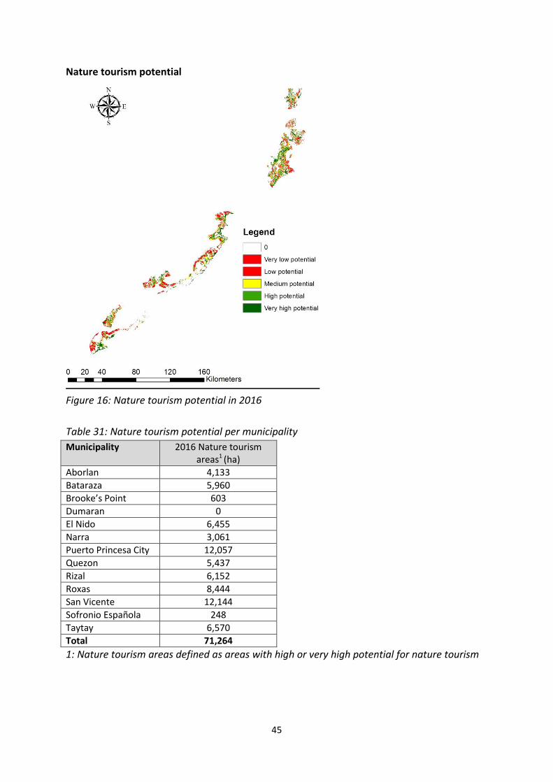
45

Nature tourism potential

Figure 16: Nature tourism potential in 2016

Table 31: Nature tourism potential per municipality

Municipality 2016 Nature tourism areas1 (ha)

Aborlan 4,133

Bataraza 5,960

Brooke’s Point 603

Dumaran 0

El Nido 6,455

Narra 3,061

Puerto Princesa City 12,057

Quezon 5,437

Rizal 6,152

Roxas 8,444

San Vicente 12,144

Sofronio Española 248

Taytay 6,570

Total 71,264

1: Nature tourism areas defined as areas with high or very high potential for nature tourism

46

4.3 Land products: 2000-2014

GPP and NPP

Table 32: The annual GPP and NPP in Palawan, as a total amount, and per m2.

Year Total GPP (Tg C)1 Mean GPP (g/C/m2) Total NPP (Tg C) Mean NPP (g/C/m2)

2000 42,3 2,890 16,0 1,090

2001 40,3 2,754 14,1 963

2002 43,7 2,981 17,1 1,165

2003 42,8 2,922 16,6 1,131

2004 44,2 3,021 17,7 1,205

2005 42,5 2,899 16,7 1,140

2006 45,1 3,078 18,3 1,247

2007 42,9 2,926 16,8 1,144

2008 43,5 2,970 17,1 1,164

2009 39,6 2,705 13,8 945

2010 42,7 2,918 16,6 1,135

2011 37,4 2,554 12,7 868

2012 38,4 2,619 12,7 869

2013 37,6 2,569 12,6 863

2014 38,9 2,656 13,7 932

1: Based on a surface area of 14,649.73 km2 for Palawan (Philippines National Statistics

Coordination Board, 2014).

Figure 16: Change in NPP for the period 2009-2014, compared to the period 2000-2008.Red

pixels show significant NPP reductions of 10% or more.

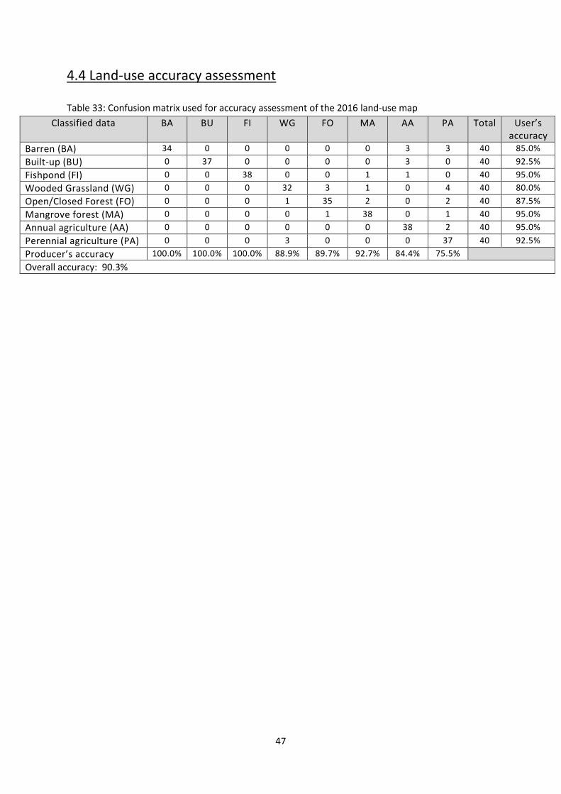
47

4.4 Land-use accuracy assessment

Table 33: Confusion matrix used for accuracy assessment of the 2016 land-use map

Classified data BA BU FI WG FO MA AA PA Total User’s accuracy

Barren (BA) 34 0 0 0 0 0 3 3 40 85.0%

Built-up (BU) 0 37 0 0 0 0 3 0 40 92.5%

Fishpond (FI) 0 0 38 0 0 1 1 0 40 95.0%

Wooded Grassland (WG) 0 0 0 32 3 1 0 4 40 80.0%

Open/Closed Forest (FO) 0 0 0 1 35 2 0 2 40 87.5%

Mangrove forest (MA) 0 0 0 0 1 38 0 1 40 95.0%

Annual agriculture (AA) 0 0 0 0 0 0 38 2 40 95.0%

Perennial agriculture (PA) 0 0 0 3 0 0 0 37 40 92.5%

Producer’s accuracy 100.0% 100.0% 100.0% 88.9% 89.7% 92.7% 84.4% 75.5%

Overall accuracy: 90.3%

48

5 DISCUSSION

Producing the land-use maps proved to be complicated and time-consuming. The 2016 land-

use map (based on Sentinel-2 data) was made first, and initial comparisons with areas that

had high-resolution data available through Google Earth showed that the accuracy appeared

to be satisfactory and consistent. However, even after applying a minimal mapping unit of

one hectare to the map, the result still showed a highly fragmented landscape. The areas

subject most to this were mountainous regions in which shadow effects caused forests to be

classified as mangrove, and in general for the wooded grassland class as the exact

boundaries of what is, and isn’t considered to be a wooded grassland are not clear-cut. As a

result, a lot of time was spent on manually rectifying the results of the land-use maps. While

this was done with the aid of high-resolution imagery, in some areas such data wasn’t

available in which case the original satellite image had to be manually interpreted.

After the production of the 2016 land-use map, the 2010 land-use map was created based

on Landsat-5 data. The same classes were chosen for this map to enable comparisons

between both land-use maps. Issues relating to the 2016 land-use map were also present

here. Additionally however, vast cloud-covered areas remained present in the Roxas and San

Vicenze municipalities, complicating an accurate classification even more. No other data

from 2010 (or late 2009/early 2011) was available for these areas, and imagery from outside

this timeframe wouldn’t be fitting for a 2010 land-use map. As a result, classifications for the

Roxas and San Vicenze municipalities have slight under- or overestimations, particularly for

the annual agriculture, wooded grassland and open forest classes. The accuracy assessment

conducted for the 2016 land-use map shows that the perennial agriculture is also very

slightly underestimated for Palawan; although most classes showed both a high user’s and

producer’s accuracy, a significant number of non-perennial pixels were classified as one. The

reason for this is twofold: first, for newly-planted perennial cropland the crops/trees are so

small, that they may not show up at all on a 10m spatial resolution imagery. As a result, such

a pixel most likely will be classified either as barren or agriculture. Second, because many

perennial crops continue to grow for many years, and spaces at which they’re planted from

one another differ between fields, the spectral signature of a perennial crop field is highly

variable. It was attempted to tackle this issue by adding several initial perennial classes.

Despite these issues that make mapping of some classes difficult, the accuracy assessment

still showed a remarkable high accuracy for many of the classes.

Interpretation of the 2016 land-use map reveals that human activities can be observed

through all of Palawan, in the form of agricultural practices, degrees of deforestation and

built-up areas. southern Palawan has a longstanding history of agricultural activity (TWG,

2015), and this is still very much evident. While annual agriculture (e.g. palay and corn)

remains the dominant form of agriculture in this region, perennial agriculture (e.g. palm oil,

coconut, coffee) is shown to be especially popular in Brooke’s Point, Sofronio Española and

areas of Rizal. The reasons for this spatial concentration of perennial activity however

49

remains unknown and would require further (social) research. For northern Palawan, annual

agriculture is found in abundance in the inland mountainous areas, with perennial

agriculture focussed near the coastlines. Wooded Grasslands throughout all of Palawan

appear near agricultural activities and is shown to often function as a transition area

between agriculture and dense forest vegetation. Although most of the forest vegetation on

Palawan is present as an open forest, more pristine, closed forests can be found particularly

in mountainous areas. Mangrove forests are located all throughout the island, but are found

to be especially common in the South (i.e. Bataraza, Rizal), near Puerto Princesa, and further

up North in Taytay. Fishponds, albeit constituting only a very small portion of the surface

area of Palawan, are particularly present in Quezon, Narra, Puerto Princesa City and Sofronio

Española. When comparing these findings with results of the 2010 land-use classification

map, the following interesting patterns emerged:

(1) Throughout all of the island, overall vegetation cover has been decreasing since

2010. When grouping vegetation classes such as wooded grassland, open forest

and closed forest together, their cover has decreased by 25,504 ha.,

approximating to around 3.0% of the initial cover in 2010. The main land

conversion consisted of agricultural land. The most alarming changes for this

occurred in northern Palawan where a high amount wooded grassland in

mountainous inland areas was converted into annual agriculture. For southern

Palawan, changes were more subtle, with existing agricultural fields further

expanding inwards at the cost of wooded grassland.

(2) In southern Palawan, particularly in Brooke’s Point, Sofronio Española, Rizal and

Narra, annual agriculture decreased drastically. The vast majority of these land

conversions resulted in an increase in perennial agriculture. In a few cases, such

as north-east Narra, patches of annual agriculture also were reforested into

wooded grassland. This pattern of land-use conversion wasn’t observable in

northern Palawan.

(3) When grouping the open and closed forest classes together, their total cover

reduced by 8,355 ha. The vast majority of these conversions led to a conversion

to wooded grassland. This is particularly in Roxas, Narra, Sofronio Española and

Quezon. When comparing the open and closed forest classes with each other,

approximately 24,000 ha. of open forest changed into closed forest. It is not sure

what this change can be attributed too, although it could be a result of yearlong

efforts towards sustainable management of ecosystems that paid off. However,

it should be noted that the S2REP forest density mapping approach used in this

research had limited accuracy due to the very influential effect of shadow as a

result of the mountainous geography.

50

(4) Increases in mangrove forests and fishponds were also observed. However, due

to limited mapping accuracy in northern Palawan in 2010, it is highly likely that

the surface area for these two classes in 2010 was significantly underestimated.

Based on these findings, the land-use maps are evidence of the continuation of a decrease

in environmental quality on Palawan (as previously argued by TWG, 2015), and thereby

further emphasize the need for additional efforts for the sustainable management of

ecosystems. In future years, it’s expected conversions from annual to perennial agriculture

continue to happen as international demands for these products remain high. Further

environmental degradation is especially expected in northern Palawan through land

conversions into annual agriculture.

Research on the ecosystem services on Palawan brought forward several key findings. Food

production likely has increased for the northern provinces of Roxas, Dumaran, San Vicente,

Taytay and Puerto Princesa. However, due to significant land conversions in southern

Palawan, overall food production still was found to have decreased by 20,144 ha. For

perennial production, an overall increase of 24,419 ha. was found. This increase occurred for

virtually all municipalities of Palawan, indicating that while conversion of annual agriculture

is common on Palawan, conversion of perennial agriculture is not. This seems plausible, as

perennial cropland usually is cultivated for 20 to 30 years, making it financially unfavourable

to convert recently-planted perennial cropland.

Research on the carbon dynamics found a slight increase of 7.77 million tons C for the

carbon stocks, despite an overall vegetation cover decrease for Palawan. This increase in

carbon stocks can be primarily attributed to the conversion of open into closed forests, but

also the increase in mangrove forests that most likely was caused by a limited accuracy of

the 2010 land-use map. When it is assumed that the surface area mangrove forests

remained constant in recent years, this would mean the carbon stocks only increased by

0.49 million tons C. Carbon stocks were found to increase throughout all of Palawan, but

with the Quezon municipality in particular. This change was brought forward as a result of a

combined decrease of annual and perennial agriculture, and an increase in closed forest

cover. For carbon sequestration, it’s estimated that land-use conversions led to a decrease

of 0.07 million tons C uptake per year, with no major changes in any of the municipalities.

The cause for the slight downward trend in carbon sequestration can be linked to the

conversion of wooded grassland to annual and perennial agriculture.

Analysis on the erosion risk on Palawan showed harmful effects of the ongoing agricultural

expansion. Areas with considerable (i.e. high and very high) erosion risk were quantified in

hectares. Due to the mountainous geography, most of these high-risk areas are located in

northern Palawan. While all of Palawan had 50,463 ha. of areas at significant risk, the

municipalities north of Puerto Princesa City contributed significantly to this with 30,204 ha.

51

These findings emphasize needs for particular sustainable management strategies in

agricultural systems in northern Palawan, to avoid long-term detrimental effects from the

agricultural expansion.

Through the analysis of agricultural potential, while suitable areas have largely been

exhausted already in municipalities with a high degree of agriculture (e.g. Bataraza, Brooke’s

Point, Sofronio Española and Narra) many opportunities clearly remained in Rizal, Aborlan,

Puerto Princesa City, and in northern Palawan. These favourable areas particularly present

themselves as wooded grassland vegetation in low-sloped areas.

From the nature tourism assessment, southern Palawan clearly holds little nature tourism

potential, primarily because most of the accessible, low-sloped areas already have been

converted to annual and perennial agriculture, and fishponds. Meanwhile, the more pristine

ecosystems in northern Palawan led to much high values for this potential. Particularly San

Vicenze, Taytay and El Nido received high scores due to the abundance and relative good

accessibility of tropical and mangrove forests. However, quantifying the potential of nature

tourism proved to be fairly complicated as some factors that influence tourism remained

unaccounted for. For instance, while parameters were used relating to the proximity to the

nearest city, Palawan’s most popular tourist attraction, the Sabang underwater caverns, is

located at a 1.5h drive away from the nearest city. Findings from the nature tourism

ecosystem service map therefore should only be seen as a first indication of this potential,

that requires further investigation to be mapped more accurately.

Some of the small fluctuations in the GPP and NPP data can be attributed to high prevalence

of cloud cover, while extremes often are the result of weather anomalies. Despite this

however, a consistent pattern showing a general decrease in GPP and NPP on Palawan can

be observed from the data. When comparing this data with the land-use maps, likely

explanations include both natural, and human-induced causes. For human-induced causes, a

likely explanation for the decrease in GPP and NPP is the expansion of perennial cropland.

For cropland such as palm oil fields, it has been shown to be a common practice to remove

parts of the wooded grassland vegetation to expand the agricultural land. Research has

shown that perennial cropland have consistently lower GPP and NPP values than natural

vegetation. For annual agriculture that has been converted back into wooded grassland, not

enough time may have passed for the ecosystem to recover and achieve normal GPP and

NPP values. Proof of natural causes contributing to this decrease as well are evident from

general GPP and NPP decreases in pristine forest ecosystems, amounting to 10 to 20%.

These findings show that even ecosystems untouched by human activities, still are taking up

considerably less carbon nowadays, than before. While no case-specific study goes into

detail on this trend, a general consensus in scientific studies for this is that events such as

changing rainfall patterns, more prominent droughts as well as ageing forests may play a

52

role in this. To better understand the exact causes for this trend on Palawan, research with a

different focus can contribute to it.

In a general context, a challenge of remotely sensed studies is the difficulty with accurately

quantifying and analysing ecosystem services. Some ecosystem services call for the inclusion

of very case-specific field data, such as measurements in the carbon dynamics, precipitation,

soil moisture levels, or tourism statistics. This thesis largely bypassed these issues by only

selecting ecosystem services that can reasonably be analysed through remote sensing, and

by obtaining as much information as possible through literature review. The main limitation

of the land-use maps relate to the limitations of optical remote sensing data. The Sentinel-2

and Landsat-5 satellite imagery only provide reflectance values for the visible and infrared

light spectrum. While this is satisfactory in analysing general land-use classes, such as

agriculture and forest vegetation, further distinction between for example the perennial

crop types remained impossible. A way to improve this in further research would be to

include Synthetic Aperture Radar (SAR) data. A limitation of the 2010 land-use map

presented itself in the significant atmospheric distortions in northern Palawan. While correct

data was still largely salvageable, underestimations of mangrove forests and fishponds

occurred. A final minor limitation was brought forward by the need of combining satellite

imagery from many different months; for instance, for the 2016 land-use map some data

from April and May had to be imported to make classification for the entire island possible.

However, this could’ve resulted in small under- or overestimations for the land-use classes.

53

6 CONCLUSION AND FUTURE RESEARCH

Palawan is a province and island in the Philippines, with a strong representation of natural

ecosystems, including many tropical and mangrove forests that constitute critical ecological

features. At the same time, human activities have started to become visible on Palawan in

recent decades, through the expansion of annual cropland such as palay and corn, and

perennial cropland such as palm oil and coconut farms. As geographical data on the

ecosystems on Palawan remains limited, the aim of this research was to produce this data by

means of analysing remotely sensed data. The objective of the research was threefold: (i) to

produce land-use maps for 2010 and 2016 for Palawan on the basis of Landsat-5 and

Sentinel-2 data, and analyse findings from these maps; (ii) studying ecosystem services on

Palawan, by combining the produced land-use maps with a Digital Elevation Model, and (iii)

to provide an accuracy assessment for the 2016 land-use map. Land-use maps for 2010 and

2016 were obtained through a series of operations in ERDAS IMAGINE, including a

supervised classification and the use of vegetation indices for further distinguishing.

The main findings from the 2016 land-use map shows that: (i) agriculture and fishponds

dominate coastal areas in southern Palawan, and for the south-eastern municipalities in

particular; (ii) agriculture in northern Palawan overall remains limited due to the

mountainous geography, but is nonetheless abundant in areas suitable for it, such as

mountain valleys; (iii) mangrove forests can be found throughout all of Palawan, and (iv)

especially in more mountainous areas, areas of closed tropical forests can be found.

Comparisons with this map were drawn with the 2010 land-use map, showing four trends of

interest: (i) Vegetation cover (including wooded grassland) has decreased on Palawan by

25,504 ha. The main cause for this is the conversion of wooded grassland into annual

agriculture in northern Palawan; (ii) Tropical forest cover (excluding wooded grassland) has

decreased by 8,355 ha. The main cause of this is conversion of open forest into wooded

grassland in the municipalities of Roxas, Narra, Sofronio Española and Quezon; (iii)

approximately 24,000 ha. of open forest has changed into closed forest; (iv) overall, a land

conversion from annual agriculture into perennial agriculture has occurred, constituting a

total area of approximately 25,000 ha. This conversion is especially noticeable in the

southern municipalities of Brooke’s Point, Sofronio Española, Narra and Rizal. Results of the

accuracy assessment argue that perennial cropland remains difficult to accurately map on

the basis of 10m spatial resolution Sentinel-2 imagery. As a result, the surface area of

perennial cropland is expected to be slightly underestimated in this thesis.

Analysis on several ecosystem services on Palawan produced the following five findings: (i)

carbon storage has increased by 7.77 million tons C, to a total of 129.10 million tons C. This

increase can attributed to an increase in closed forest cover, as well as a slight overall

decrease in agriculture. (ii) carbon sequestration reduced by 0.07 million tons C per year, to

a total of 4.61 million tons C per year; (iii) erosion risk as a result of agricultural expansion is

especially apparent in northern Palawan, with 30,204 ha. being classified as a high-risk

54

area.; (iv) options for agricultural expansion has largely been exhausted for most southern

municipalities. However, considerable areas with potential for agriculture remain in Rizal,

Aborlan, Puerto Princesa City and the northern municipalities; and (v) due to a good

preservation of pristine ecosystems, northern Palawan with in particular San Vicenze, Taytay

and El Nido, show high potential for nature tourism.

Findings from this research emphasize the need for sustainable ecosystem management on

Palawan. Findings on the land-use and ecosystem services can assist local organizations and

policy-makers. However, this thesis doesn’t encompass any locally obtained data. For most

data on ecosystem services, findings from existing literature in comparable study areas were

obtained. As a result, produced values and statistics for Palawan should be seen as

approximations. Future research could therefore focus more on the collection of such case-

specific data. This thesis furthermore suggests for the use of radar remote sensing, such as

Synthetic Aperture Radar (SAR), to more accurately map perennial cropland as well as

mapping the different perennial crop types. Other remote sensing methods can be used to

more accurately map the density of forest vegetation on Palawan, which was found to be

difficult and in some cases unreliable through optical remote sensing. However, given the

context of the research of relying on a limited supply of data, this thesis shows interesting

results that can contribute to the scientific discussion.

55

7 BIBLIOGRAPHY

1. Adame, M. F., Kauffman, J. B., Medina, I., Gamboa, J. N., Torres, O., Caamal, J. P., ... & Herrera-Silveira, J. A. (2013). Carbon stocks of tropical coastal wetlands within the karstic landscape of the Mexican Caribbean. PLoS One, 8(2), e56569.

2. Alongi, D. M. (2014). Carbon cycling and storage in mangrove forests. Annual review of marine science, 6, 195-219.

3. Andreae, M. O., Artaxo, P., Brandao, C., Carswell, F. E., Ciccioli, P., Da Costa, A. L., ... & Kabat, P. (2002). Biogeochemical cycling of carbon, water, energy, trace gases, and aerosols in Amazonia: The LBA‐EUSTACH experiments. Journal of Geophysical Research: Atmospheres, 107(D20).

4. Assessment, M. E. (2005). Millennium ecosystem assessment. Ecosystems and Human Well-Being: Biodiversity Synthesis, Published by World Resources Institute, Washington, DC.

5. Ayanu, Y. Z., Conrad, C., Nauss, T., Wegmann, M., & Koellner, T. (2012). Quantifying and mapping ecosystem services supplies and demands: a review of remote sensing applications. Environmental science & technology, 46(16), 8529-8541.

6. Basri, H., Ali, S. A., & Kasuri, A. R. (2015, November). How to restore the Tropical Peat Swamp Forest in Aceh Province, Indonesia. In Proceedings of The Annual International Conference, Syiah Kuala University-Life Sciences & Engineering Chapter (Vol. 5, No. 2).

7. Bateman, I. J., Mace, G. M., Fezzi, C., Atkinson, G., & Turner, K. (2011). Economic analysis for ecosystem service assessments. Environmental and Resource Economics, 48(2), 177-218.

8. Bhattacharyya, T., Chandran, P., Ray, S. K., Mandal, C., Tiwary, P., Pal, D. K., ... & Sahrawat, K. L. (2014). Processes determining the sequestration and maintenance of carbon in soils: a synthesis of research from tropical India. Soil Horizons, 55(4).

9. Birdsey, R., Pregitzer, K., & Lucier, A. (2006). Forest carbon management in the United States. Journal of environmental quality, 35(4), 1461-1469.

10. Bouvet, G., Ferraris, J., & Andréfouët, S. (2003). Evaluation of large-scale unsupervised classification of New Caledonia reef ecosystems using Landsat 7 ETM+ imagery. Oceanologica Acta, 26(3), 281-290.

11. Braat, L. C., & de Groot, R. (2012). The ecosystem services agenda: bridging the worlds of natural science and economics, conservation and development, and public and private policy. Ecosystem Services, 1(1), 4-15.

12. Brooks, T. M., Mittermeier, R. A., da Fonseca, G. A., Gerlach, J., Hoffmann, M., Lamoreux, J. F., ... & Rodrigues, A. S. (2006). Global biodiversity conservation priorities. science, 313(5783), 58-61.

13. Brown, S., & Lugo, A. E. (1984). Biomass of tropical forests: a new estimate based on forest volumes. Science, 223, 1290-1294.

14. Bouillon, S., Borges, A. V., Castañeda‐Moya, E., Diele, K., Dittmar, T., Duke, N. C., ... & Rivera‐Monroy, V. H. (2008). Mangrove production and carbon sinks: a revision of global budget estimates. Global Biogeochemical Cycles, 22(2).

15. Ceschia, E., Béziat, P., Dejoux, J. F., Aubinet, M., Bernhofer, C., Bodson, B., ... & Elbers, J. A. (2010). Management effects on net ecosystem carbon and GHG budgets at European crop sites. Agriculture, ecosystems & environment, 139(3), 363-383.

56

16. Clark, K. L., Gholz, H. L., & Castro, M. S. (2004). Carbon dynamics along a chronosequence of slash pine plantations in north Florida. Ecological Applications, 14(4), 1154-1171.

17. Costanza, R., de Groot, R., Sutton, P., van der Ploeg, S., Anderson, S. J., Kubiszewski,

I., ... & Turner, R. K. (2014). Changes in the global value of ecosystem services. Global

Environmental Change, 26, 152-158.

18. Daily, G. C., Matson, P. A., & Vitousek, P. M. (1997). Ecosystem services supplied by

soil. Nature’s services: societal dependence on natural ecosystems, 113-132.

19. Davis, F. W., & Michaelsen, J. (1995). Sensitivity of fire regime in chaparral ecosystems to climate change. In Global change and Mediterranean-type ecosystems (pp. 435-456). Springer New York.

20. De Groot, R. S., Wilson, M. A., & Boumans, R. M. (2002). A typology for the classification, description and valuation of ecosystem functions, goods and services. Ecological economics, 41(3), 393-408.

21. De Groot, R. S., Alkemade, R., Braat, L., Hein, L., & Willemen, L. (2010). Challenges in integrating the concept of ecosystem services and values in landscape planning, management and decision making. Ecological complexity, 7(3), 260-272.

22. Dixon, R. K., Winjum, J. K., Andrasko, K. J., Lee, J. J., & Schroeder, P. E. (1994).

Integrated land-use syste

23. Dobson, A., Lodge, D., Alder, J., Cumming, G. S., Keymer, J., McGlade, J., ... & Wall, D. (2006). Habitat loss, trophic collapse, and the decline of ecosystem services. Ecology, 87(8), 1915-1924.

24. Donato, D. C., Kauffman, J. B., Murdiyarso, D., Kurnianto, S., Stidham, M., & Kanninen, M. (2011). Mangroves among the most carbon-rich forests in the tropics. Nature Geoscience, 4(5), 293-297.

25. Dung, I. D., & Mohan, D. R. (2016). Analysis of Tourist Satisfaction with Tourism Products in Andaman and Nicobar Islands. St Theresa Journal of Humanities and Social Sciences, 2(1).

26. Ervin, D. E., Brown, D., Chang, H., Dujon, V., Granek, E. F., Shandas, V., & Yeakley, J. A. (2012). Growing cities depend on ecosystem services. Solutions: For a Sustainable and Desirable Future.

27. Estoque, R. C., & Murayama, Y. (2012). Examining the potential impact of land-use/cover changes on the ecosystem services of Baguio city, the Philippines: a scenario-based analysis. Applied Geography, 35(1), 316-326.

28. Fisher, B., Turner, R. K., & Morling, P. (2009). Defining and classifying ecosystem services for decision making. Ecological economics, 68(3), 643-653.

29. Foley, J. A., Asner, G. P., Costa, M. H., Coe, M. T., DeFries, R., Gibbs, H. K., ... & Snyder, P. (2007). Amazonia revealed: forest degradation and loss of ecosystem goods and services in the Amazon Basin. Frontiers in Ecology and the Environment, 5(1), 25-32.

30. Forest Resource Assessment (FAO) (2005) Progress towards sustainable forest management. Accessed 11 December 2016. Retrieved from: http://www.fao.org/docrep/008/a0400e/a0400e00.htm

31. Frolking, S., Talbot, J., & Subin, Z. M. (2014). Exploring the relationship between peatland net carbon balance and apparent carbon accumulation rate at century to millennial time scales. The Holocene, 24(9), 1167-1173.

57

32. Germer, J., & Sauerborn, J. (2008). Estimation of the impact of oil palm plantation establishment on greenhouse gas balance. Environment, Development and Sustainability, 10(6), 697-716.

33. Gibbs, H. K., Brown, S., Niles, J. O., & Foley, J. A. (2007). Monitoring and estimating tropical forest carbon stocks: making REDD a reality. Environmental Research Letters, 2(4), 045023.

34. Gilmanov, T. G., Coughenour, M. B., Ojima, D. S., Scurlock, J. M. O., Scholes, R. J., Hall, D. O., ... & Kinyamario, J. I. (1996). Global grassland ecosystem modelling: development and test of ecosystem models for grassland systems.

35. Gobena, Y. J. (2003). Soil Erosion Assessment Using Remotely Sensed Data and Ancillary Data in the Desert Of Tabernas, southeast Spain. ITC. Netherlands.

36. Goetz, S. J., Baccini, A., Laporte, N. T., Johns, T., Walker, W., Kellndorfer, J., ... & Sun, M. (2009). Mapping and monitoring carbon stocks with satellite observations: a comparison of methods. Carbon balance and management, 4(1), 2.

37. Gomez, C., Rossel, R. A. V., & McBratney, A. B. (2008). Soil organic carbon prediction by hyperspectral remote sensing and field vis-NIR spectroscopy: An Australian case study. Geoderma, 146(3), 403-411.

38. Hein, L., Van Koppen, K., De Groot, R. S., & Van Ierland, E. C. (2006). Spatial scales, stakeholders and the valuation of ecosystem services. Ecological economics, 57(2), 209-228.

39. Helliwell, D. R. (1969). Valuation of wildlife resources. Regional studies, 3(1), 41-47. 40. Hirano, T., Segah, H., Harada, T., Limin, S., June, T., Hirata, R., & Osaki, M. (2007).

Carbon dioxide balance of a tropical peat swamp forest in Kalimantan, Indonesia. Global Change Biology, 13(2), 412-425.

41. Hopkinson, C., Chasmer, L., Colville, D., Fournier, R. A., Hall, R. J., Luther, J. E., ... & St-Onge, B. (2013). Moving toward consistent ALS monitoring of forest attributes across Canada. Photogrammetric Engineering & Remote Sensing, 79(2), 159-173.

42. Iqbal, F. (2011). Detection of salt affected soil in rice-wheat area using satellite image. African Journal of Agricultural Research, 6(21), 4973-4982

43. IRRI and PhilRice (n.d.) Cropping Calendar. Accessed 28 November 2017. Retrieved from: http://philfsis.psa.gov.ph/index.php/id/24/prov/1753

44. Jensen, J. R., & Lulla, K. (1987). Introductory digital image processing: a remote sensing perspective.

45. Jensen, M. E., Bourgeron, P., Everett, R., & Goodman, I. (1996). ECOSYSTEM MANAGEMENT: A LANDSCAPE ECOLOGY PERSPECTWE1.

46. Kauffman, J. B., Heider, C., Cole, T. G., Dwire, K. A., & Donato, D. C. (2011). Ecosystem carbon stocks of Micronesian mangrove forests. Wetlands, 31(2), 343-352.

47. Kempka, R. G., Kollasch, R. P., & Koeln, G. T. (1992). Ducks Unlimited: Using GIS to preserve the Pacific Flyway’s wetland resource. GIS World, 5, 46-52.

48. Kendall, M. S., & Miller, T. (2008). The influence of thematic and spatial resolution on maps of a coral reef ecosystem. Marine Geodesy, 31(2), 75-102.

49. Kerr, J. T., & Ostrovsky, M. (2003). From space to species: ecological applications for remote sensing. Trends in Ecology & Evolution, 18(6), 299-305.

50. King, A. R., & Brownell, J. A. (1966). The curriculum and the disciplines of knowledge (p. 86). New York: Wiley.

58

51. Kreuter, U. P., Harris, H. G., Matlock, M. D., & Lacey, R. E. (2001). Change in ecosystem service values in the San Antonio area, Texas. Ecological economics, 39(3), 333-346.

52. Kroodsma, D. A., & Field, C. B. (2006). Carbon sequestration in California agriculture, 1980–2000. Ecological Applications, 16(5), 1975-1985.

53. Kwarteng, P. S., & Chavez, A. Y. (1989). Extracting spectral contrast in Landsat Thematic Mapper image data using selective principal component analysis. Photogramm. Eng. Remote Sens, 55, 339-348.

54. Lal, R. (2004). Soil carbon sequestration impacts on global climate change and food security. science, 304(5677), 1623-1627.

55. Lasco, R. D., & Pulhin, F. B. (2003). Philippine forest ecosystems and climate change: carbon stocks, rate of sequestration and the Kyoto Protocol. Annals of Tropical Research, 25(2), 37-51.

56. Law, E. A., Bryan, B. A., Meijaard, E., Mallawaarachchi, T., Struebig, M., & Wilson, K. A. (2015). Ecosystem services from a degraded peatland of Central Kalimantan: implications for policy, planning, and management. Ecological Applications, 25(1), 70-87.

57. Liu, J., Li, S., Ouyang, Z., Tam, C., & Chen, X. (2008). Ecological and socioeconomic effects of China's policies for ecosystem services. Proceedings of the National academy of Sciences, 105(28), 9477-9482.

58. Liao, C., Luo, Y., Jiang, L., Zhou, X., Wu, X., Fang, C., ... & Li, B. (2007). Invasion of Spartina alterniflora enhanced ecosystem carbon and nitrogen stocks in the Yangtze Estuary, China. Ecosystems, 10(8), 1351-1361.

59. Lobell, D. B. (2013). The use of satellite data for crop yield gap analysis. Field Crops Research, 143, 56-64.

60. Lugo, A. E., & Brown, S. (1992). Tropical forests as sinks of atmospheric carbon. Forest Ecology and Management, 54(1-4), 239-255.

61. Lu, M., Zhou, X., Yang, Q., Li, H., Luo, Y., Fang, C., ... & Li, B. (2013). Responses of ecosystem carbon cycle to experimental warming: a meta‐analysis. Ecology, 94(3), 726-738.

62. Macleod, R. D., & Congalton, R. G. (1998). A quantitative comparison of change-detection algorithms for monitoring eelgrass from remotely sensed data. Photogrammetric engineering and remote sensing, 64(3), 207-216.

63. Malhi, Y., Nobre, A. D., Grace, J., Kruijt, B., Pereira, M. G., Culf, A., & Scott, S. (1998). Carbon dioxide transfer over a Central Amazonian rain forest. Journal of Geophysical Research: Atmospheres, 103(D24), 31593-31612.

64. Miettinen, J., Shi, C., Tan, W. J., & Liew, S. C. (2012). 2010 land cover map of insular Southeast Asia in 250-m spatial resolution. Remote Sensing Letters, 3(1), 11-20.

65. Mizoguchi, Y., Ohtani, Y., Takanashi, S., Iwata, H., Yasuda, Y., & Nakai, Y. (2012). Seasonal and interannual variation in net ecosystem production of an evergreen needleleaf forest in Japan. Journal of forest research, 17(3), 283-295.

66. Murdiyarso, D., Purbopuspito, J., Kauffman, J. B., Warren, M. W., Sasmito, S. D., Donato, D. C., ... & Kurnianto, S. (2015). The potential of Indonesian mangrove forests for global climate change mitigation. Nature Climate Change, 5(12), 1089-1092.

59

67. Naidoo, R., Balmford, A., Costanza, R., Fisher, B., Green, R. E., Lehner, B., ... & Ricketts, T. H. (2008). Global mapping of ecosystem services and conservation priorities. Proceedings of the National Academy of Sciences, 105(28), 9495-9500.

68. Ojha, V. P. (2009). Carbon emissions reduction strategies and poverty alleviation in India. Environment and Development Economics, 14(03), 323-348.

69. Ozesmi, S. L., & Bauer, M. E. (2002). Satellite remote sensing of wetlands. Wetlands ecology and management, 10(5), 381-402.

70. Pan, G., Li, L., Wu, L., & Zhang, X. (2004). Storage and sequestration potential of topsoil organic carbon in China's paddy soils. Global Change Biology, 10(1), 79-92.

71. Pareta, K. (2013). Assessment of Carbon Stocks in Shifting Cultivation Lands: A Case Study of Nagaland State of India. In Esri International user conference (pp. 2-20).

72. Pearce, D. W., & Atkinson, G. D. (1993). Capital theory and the measurement of sustainable development: an indicator of “weak” sustainability. Ecological economics, 8(2), 103-108.

73. Pimentel, D., Berger, B., Filiberto, D., Newton, M., Wolfe, B., Karabinakis, E., ... & Nandagopal, S. (2004). Water resources: agricultural and environmental issues. BioScience, 54(10), 909-918.

74. Potter, C., Klooster, S., Hiatt, C., Genovese, V., & Castilla-Rubio, J. C. (2011). Changes in the carbon cycle of Amazon ecosystems during the 2010 drought. Environmental Research Letters, 6(3), 034024.

75. Phalan, B., Green, R. E., Dicks, L. V., Dotta, G., Feniuk, C., Lamb, A., ... & Balmford, A. (2016). How can higher-yield farming help to spare nature?. Science, 351(6272), 450-451.

76. Remme, R. P., Edens, B., Schröter, M., & Hein, L. (2015). Monetary accounting of ecosystem services: A test case for Limburg province, the Netherlands. Ecological Economics, 112, 116-128.

77. Saatchi, S., Marlier, M., Chazdon, R. L., Clark, D. B., & Russell, A. E. (2011). Impact of spatial variability of tropical forest structure on radar estimation of aboveground biomass. Remote Sensing of Environment, 115(11), 2836-2849.

78. Schröter, M., Barton, D. N., Remme, R. P., & Hein, L. (2014). Accounting for capacity and flow of ecosystem services: A conceptual model and a case study for Telemark, Norway. Ecological Indicators, 36, 539-551.

79. Scott, R. L., Huxman, T. E., Barron‐Gafford, G. A., Darrel Jenerette, G., Young, J. M., & Hamerlynck, E. P. (2014). When vegetation change alters ecosystem water availability. Global change biology, 20(7), 2198-2210.

80. Shang, Q., Yang, X., Gao, C., Wu, P., Liu, J., Xu, Y., ... & Guo, S. (2011). Net annual global warming potential and greenhouse gas intensity in Chinese double rice‐cropping systems: a 3‐year field measurement in long‐term fertilizer experiments. Global Change Biology, 17(6), 2196-2210.

81. Singh, H., Kumar, M., Joshi, M., & Chisanga, K. (2012). Soil Carbon Stock and its Role in Carbon Sequestration. GLIMPSES OF FORESTRY RESEARCH IN THE INDIAN HIMALAYAN REGION, 89.

82. Song, G., Li, L., Pan, G., & Zhang, Q. (2005). Topsoil organic carbon storage of China and its loss by cultivation. Biogeochemistry, 74(1), 47-62.

83. Southern Palawan Technical Working Group (TWG) (2015) Pilot Ecosystem Account for Southern Palawan.

60

84. Sumarga, E., & Hein, L. (2014). Mapping ecosystem services for land-use planning, the case of Central Kalimantan. Environmental management, 54(1), 84-97.

85. The Economics of Ecosystems & Biodiversity (TEEB)(2010) Ecological and Economic Foundations. Accessed 14 August 2016. Retrieved from: http://www.teebweb.org/our-publications/teeb-study-reports/ecological-and-economic-foundations/

86. Verburg, P. H. (2006). Simulating feedbacks in land-use and land cover change models. Landscape Ecology, 21(8), 1171-1183.

87. Vitousek, P. M., Mooney, H. A., Lubchenco, J., & Melillo, J. M. (1997). Human domination of Earth's ecosystems. Science, 277(5325), 494-499.

88. Waddington, J. M., Griffis, T. J., & Rouse, W. R. (1998). Northern Canadian wetlands: net ecosystem CO2 exchange and climatic change. Climatic change, 40(2), 267-275.

89. WCED (1987) Report of the World Commission on Environment and Development: Our Common Future. Accessed 17 November, 2016. Retrieved from: http://www.un-documents.net/wced-ocf.htm

90. Weng, Q. (2001). A remote sensing? GIS evaluation of urban expansion and its impact on surface temperature in the Zhujiang Delta, China. International journal of remote sensing, 22(10), 1999-2014.

91. Xie, G., & Steinberger, Y. (2001). Temporal patterns of C and N under shrub canopy in a loessial soil desert ecosystem. Soil Biology and Biochemistry, 33(10), 1371-1379.

92. Xu, X., Thornton, P. E., & Post, W. M. (2013). A global analysis of soil microbial biomass carbon, nitrogen and phosphorus in terrestrial ecosystems. Global Ecology and Biogeography, 22(6), 737-749.

93. Zha, T., Barr, A. G., van der Kamp, G., Black, T. A., McCaughey, J. H., & Flanagan, L. B. (2010). Interannual variation of evapotranspiration from forest and grassland ecosystems in western Canada in relation to drought. Agricultural and Forest Meteorology, 150(11), 1476-1484.Barr

94. Zheng, X., Xie, B., Liu, C., Zhou, Z., Yao, Z., Wang, Y., ... & Butterbach‐Bahl, K. (2008). Quantifying net ecosystem carbon dioxide exchange of a short‐plant cropland with intermittent chamber measurements. Global Biogeochemical Cycles, 22(3).