IMRN International Mathematics Research Notices1996, No. 1

A Relationship between Poincare-Type Inequalities and

Representation Formulas in Spaces of Homogeneous Type

Bruno Franchi, Guozhen Lu, and Richard L. Wheeden

The purpose of this note is to study the relationship between the validity of L1 versions

of Poincare’s inequality and the existence of representation formulas for functions as

(fractional) integral transforms of first-order vector fields.

The simplest example of a representation formula of the type we have in mind is

the following familiar inequality for a smooth, real-valued function f(x) defined on a ball

B in N-dimensional Euclidean space RN:

|f(x)− fB| ≤ C∫B

|∇f(y)||x− y|N−1

dy, x ∈ B,

where ∇f denotes the gradient of f, fB is the average |B|−1∫Bf(y)dy, |B| is the Lebesgue

measure of B, and C is a constant which is independent of f, x, B.

We are primarily interested in showing that various analogues of the formula

above for more general systems of first-order vector fields Xf = (X1f, . . . , Xmf) are simple

corollaries of (and, in fact, often equivalent to) appropriate L1 Poincare inequalities of

the form

1

ν(B)

∫B

|f− fB,ν|dν ≤ Cr(B)1

µ(B)

∫B

|Xf|dµ. (1)

Here ν and µ are measures, B is a ball of radius r(B) with respect to a metric that is

naturally associated with the vector fields, and fB,ν = ν(B)−1∫Bf dν.

Recently, representation formulas inRN were derived for Hormander vector fields

in [FLW] (see also [L1]) as well as for some nonsmooth vector fields of Grushin type in

[FGW]. In the case of Hormander vector fields, if ρ(x, y) denotes the associated metric (see

[FP], [NSW], [San]) and B(x, r) denotes the metric ball with center x and radius r, then we

Received 30 August 1995. Revision received 22 September 1995.Communicated by Carlos Kenig.

2 Franchi, Lu, and Wheeden

have the representation formula (derived in [FLW])

|f(x)− fB| ≤ C∫τB

|Xf(y)| ρ(x, y)

|B(x, ρ(x, y))| dy (2)

for x ∈ B and τ > 1, where τB is the ball concentric with B of radius τr(B).

If a representation formula like (2) holds, then we can repeat our arguments in

[FLW] to obtain two-weight Lp, Lq Sobolev-Poincare inequalities. As is shown in [FLW,

Section 4], these inequalities lead to relative isoperimetric estimates for Hormander vec-

tor fields, or even for nonsmooth vector fields as in [FL], [F], [FGW].

The proof of (2) in [FLW] consists of an elaborate argument relying directly on the

lifting procedure introduced by Rothschild and Stein [RS], whereas it will follow from

our main result that (2) is equivalent to the Poincare estimate (1) when both ν and µ are

chosen to be Lebesgue measure. Since this form of (1) is known to be true (the argument

given in Jerison [J] for the L2 version of Poincare’s inequality for Hormander vector fields

and Lebesgue measure also works for the L1 version), we thus obtain a proof of (2) that

is shorter than the one given in [FLW].

As we shall see, the equivalence between estimates like (1) and (2) holds in a very

general context and can be applied to different situations. This fact stresses once more

the central role played by Poincare’s inequality in many problems. The simple technique

we will use to show that Poincare’s inequality leads to a representation formula is based

on some modifications in an argument due to Lotkowski and the third author [LW]. The

method works in any homogeneous space in the sense of Coifman and Weiss [CW], i.e.,

in any quasimetric space equipped with a doubling measure. Moreover, the method does

not require the presence of a derivation operator Xf on the right-hand side of either (1) or

the representation formula: any function can be used, as we will see in Remark 1 below.

After this paper was submitted for publication, the authors received a preprint

of the note [CDG2] containing another proof of the representation formula (2), relying

on Jerison’s Poincare inequality, on the notion of “subelliptic mollifiers” introduced in

[CDG1], and on the estimates for the fundamental solution and its derivatives for sums-

of-squares operators proved in [NSW] and [San]. Our present results do not require any

differential structure or vector field context, and so also do not require estimates for the

fundamental solutions of differential operators.

For a homogeneous space (S, ρ,m), ρ denotes a quasimetric with quasimetric con-

stant K; i.e., for all x, y, z ∈ S,

ρ(x, y) ≤ K [ρ(x, z)+ ρ(z, y)],

and m is a doubling measure; i.e., there is a constant c such that

m(B(x, 2r)) ≤ cm(B(x, r)), x ∈ S, r > 0,

Poincare-Type Inequalities and Representation Formulas 3

where, by definition, B(x, r) = {y ∈ S : ρ(x, y) < r}, and m(B(x, r)) denotes the m-measure of

B(x, r). As usual,we refer to B(x, r) as the ball with center x and radius r, and if B is a ball,

we write xB for its center, r(B) for its radius, and cB for the ball of radius cr(B) having the

same center as B.

We now state and prove our main result, showing when Poincare’s inequality

implies a representation formula. The reverse implication, namely, results showing when

representation formulas lead to L1 Poincare estimates, can be easily derived by using

Fubini’s theorem. We briefly discuss this in Theorem 2 below; see also the remarks at

the end of Section 3 of [FLW]. Finally, some examples of applications of the theorems are

listed at the end of the paper. In these examples, ρ(x, y) is actually a metric, and so Kmay

be taken to be 1.

Let us state now our main result.

Theorem 1. Let ν, µ be doubling measures on a homogeneous space (S, ρ,m). Let B0 be

a ball, τ > 1, ε > 0, and assume for all balls B ⊂ τKB0 (K is the quasimetric constant) that

1

ν(B)

∫B

|f− fB,ν|dν ≤ Cr(B)1

µ(B)

∫B

|Xf|dµ, (1.a)

where f is a given function on τKB0, and that for all balls B, B with B ⊂ B ⊂ τKB0,

r(B)µ(B)

≤ C(r(B)

r(B)

)εr(B)

µ(B), (1.b)

or equivalently,

µ(B) ≥ c(r(B)

r(B)

)1+εµ(B).

Then, for ν–almost every x ∈ B0,

|f(x)− fB0,ν| ≤ C∫τKB0

|Xf(y)| ρ(x, y)

µ(B(x, ρ(x, y)))dµ(y) (1.c)

with fB0,ν = ν(B0)−1∫B0f dν.

On the right sides of (1.a) and (1.c), we have used the vector field notation Xf,

but any function will do; see the first remark which follows the proof for slightly more

general forms of Theorem 1.

4 Franchi, Lu, and Wheeden

Proof. By hypothesis, for fixed τ > 1 and all balls B ⊂ τKB0,

1

ν(B)

∫B

|f− fB|dν ≤ C r(B)

µ(B)

∫B

|Xf|dµ,

where for simplicity we have written fB for fB,ν. Let x ∈ B0. There is a constant η > 0

independent of x and B0 such that B(x, ηr(B0)) ⊂ τKB0: in fact, it is enough to choose η

such that 1+ η < τ, since if y ∈ B(x, ηr(B0)), then

ρ(xB0 , y) ≤ K (ρ(xB0 , x)+ ρ(x, y))

≤ K (r(B0)+ ηr(B0)) = K(1+ η)r(B0)

< Kτr(B0).

Denote B(x, ηr(B0)) = B1. Then r = r(B1) = ηr(B0). Now

|f(x)− fB0 | ≤ |f(x)− fB1 | + |fB1 − fB0 |. (3)

For the second term on the right of (3), we have

|fB1 − fB0 | ≤ |fB1 − fτKB0 | + |fB0 − fτKB0 |

≤ 1ν(B1)

∫B1

|f(y)− fτKB0 |dν(y)+ 1ν(B0)

∫B0

|f(y)− fτKB0 |dν(y)

≤(

1

ν(B1)+ 1

ν(B0)

) ∫τKB0

|f(y)− fτKB0 |dν(y)

since B1, B0 ⊂ τKB0

≤ C

ν(τKB0)

∫τKB0

|f− fτKB0 |dν

since ν is doubling and r(B1), r(B0) ≈ r(τKB0)

≤ C r(τKB0)

µ(τKB0)

∫τKB0

|Xf|dµ by hypothesis (1.a)

≤ C∫τKB0

|Xf(y)| ρ(x, y)µ(B(x, ρ(x, y)))

dµ(y)

as desired, since if y ∈ τKB0, then ρ(x, y) < 2Kr(τKB0) ≈ r(B0), and then we can apply (1.b),

with B = τKB0 and B = B(x, (τ − 1)ρ(x, y)/2K2τ) (the fact that B ⊂ τKB0 follows by using

the “triangle” inequality as before), together with the doubling of µ to get

r(τKB0)

µ(τKB0)≤ C

(ρ(x, y)

r(B0)

)ερ(x, y)

µ(B(x, ρ(x, y)))≤ C ρ(x, y)

µ(B(x, ρ(x, y))).

Poincare-Type Inequalities and Representation Formulas 5

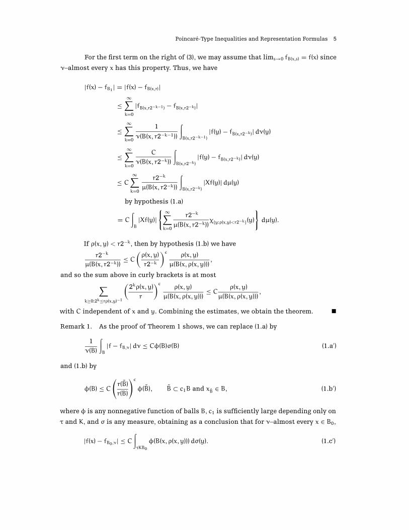
For the first term on the right of (3), we may assume that lims→0 fB(x,s) = f(x) since

ν–almost every x has this property. Thus, we have

|f(x)− fB1 | = |f(x)− fB(x,r)|

≤∞∑k=0

|fB(x,r2−k−1) − fB(x,r2−k)|

≤∞∑k=0

1

ν(B(x, r2−k−1))

∫B(x,r2−k−1)

|f(y)− fB(x,r2−k)|dν(y)

≤∞∑k=0

C

ν(B(x, r2−k))

∫B(x,r2−k)

|f(y)− fB(x,r2−k)|dν(y)

≤ C∞∑k=0

r2−k

µ(B(x, r2−k))

∫B(x,r2−k)

|Xf(y)|dµ(y)

by hypothesis (1.a)

= C∫B

|Xf(y)|{ ∞∑k=0

r2−k

µ(B(x, r2−k))χ{y:ρ(x,y)<r2−k}(y)

}dµ(y).

If ρ(x, y) < r2−k, then by hypothesis (1.b) we have

r2−k

µ(B(x, r2−k))≤ C

(ρ(x, y)

r2−k

)ερ(x, y)

µ(B(x, ρ(x, y))),

and so the sum above in curly brackets is at most∑k≥0:2k≤rρ(x,y)−1

(2kρ(x, y)

r

)ερ(x, y)

µ(B(x, ρ(x, y)))≤ C ρ(x, y)

µ(B(x, ρ(x, y))),

with C independent of x and y. Combining the estimates, we obtain the theorem.

Remark 1. As the proof of Theorem 1 shows, we can replace (1.a) by

1

ν(B)

∫B

|f− fB,ν|dν ≤ Cφ(B)σ(B) (1.a′)

and (1.b) by

φ(B) ≤ C(r(B)

r(B)

)εφ(B), B ⊂ c1B and xB ∈ B, (1.b′)

where φ is any nonnegative function of balls B, c1 is sufficiently large depending only on

τ and K, and σ is any measure, obtaining as a conclusion that for ν–almost every x ∈ B0,

|f(x)− fB0,ν| ≤ C∫τKB0

φ(B(x, ρ(x, y)))dσ(y). (1.c′)

6 Franchi, Lu, and Wheeden

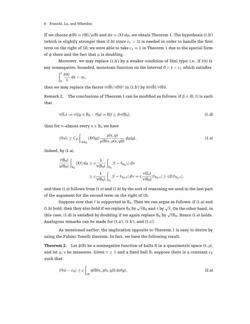
If we choose φ(B) = r(B)/µ(B) and dσ = |Xf|dµ,we obtain Theorem 1. The hypothesis (1.b′)

(which is slightly stronger than (1.b) since c1 > 1) is needed in order to handle the first

term on the right of (3); we were able to take c1 = 1 in Theorem 1 due to the special form

of φ there and the fact that µ is doubling.

Moreover, we may replace (1.b′) by a weaker condition of Dini type; i.e., if δ(t) is

any nonnegative, bounded, monotone function on the interval 0 < t < c1 which satisfies∫1

0

δ(t)tdt <∞,

then we may replace the factor (r(B)/r(B))ε in (1.b′) by δ(r(B)/r(B)).

Remark 2. The conclusions of Theorem 1 can be modified as follows: if β ∈ (0, 1) is such

that

ν(Ef) := ν({y ∈ B0 : f(y) = 0}) ≥ βν(B0), (1.d)

then for ν–almost every x ∈ B0 we have

|f(x)| ≤ Cβ∫τKB0

|Xf(y)| ρ(x, y)

µ(B(x, ρ(x, y)))dµ(y). (1.e)

Indeed, by (1.a),

r(B0)

µ(B0)

∫B0

|Xf|dµ ≥ c 1ν(B0)

∫B0

|f− fB0,ν|dν

≥ c 1ν(B0)

∫Ef

|f− fB0,ν|dν = cν(Ef)

ν(B0)|fB0,ν| ≥ cβ|fB0,ν|,

and then (1.e) follows from (1.c) and (1.b) by the sort of reasoning we used in the last part

of the argument for the second term on the right of (3).

Suppose now that f is supported in B0. Then we can argue as follows: if (1.a) and

(1.b) hold, then they also hold if we replace B0 by√τB0 and τ by

√τ. On the other hand, in

this case, (1.d) is satisfied by doubling if we again replace B0 by√τB0. Hence (1.e) holds.

Analogous remarks can be made for (1.a′), (1.b′), and (1.c′).

As mentioned earlier, the implication opposite to Theorem 1 is easy to derive by

using the Fubini-Tonelli theorem. In fact, we have the following result.

Theorem 2. Let φ(B) be a nonnegative function of balls B in a quasimetric space (S, ρ),

and let µ, ν be measures. Given τ ≥ 1 and a fixed ball B, suppose there is a constant cB

such that

|f(x)− cB| ≤ c∫τB

φ(B(x, ρ(x, y)))dσ(y), (2.a)

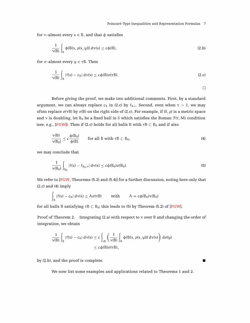
Poincare-Type Inequalities and Representation Formulas 7

for ν–almost every x ∈ B, and that φ satisfies

1

ν(B)

∫B

φ(B(x, ρ(x, y)))dν(x) ≤ cφ(B), (2.b)

for σ–almost every y ∈ τB. Then

1

ν(B)

∫B

|f(x)− cB|dν(x) ≤ cφ(B)σ(τB). (2.c)

Before giving the proof, we make two additional comments. First, by a standard

argument, we can always replace cB in (2.c) by fB,ν. Second, even when τ > 1, we may

often replace σ(τB) by σ(B) on the right side of (2.c). For example, if (S, ρ) is a metric space

and ν is doubling, let B0 be a fixed ball in S which satisfies the Boman F(τ,M) condition

(see, e.g., [FGW]). Then if (2.c) holds for all balls B with τB ⊂ B0 and if also

ν(B)

ν(B0)≤ cφ(B0)

φ(B)for all B with τB ⊂ B0, (4)

we may conclude that

1

ν(B0)

∫B0

|f(x)− fB0,ν|dν(x) ≤ cφ(B0)σ(B0). (5)

We refer to [FGW, Theorems (5.2) and (5.4)] for a further discussion, noting here only that

(2.c) and (4) imply∫B

|f(x)− cB|dν(x) ≤ Aσ(τB) with A = cφ(B0)ν(B0)

for all balls B satisfying τB ⊂ B0; this leads to (5) by Theorem (5.2) of [FGW].

Proof of Theorem 2. Integrating (2.a) with respect to ν over B and changing the order of

integration, we obtain

1ν(B)

∫B

|f(x)− cB|dν(x) ≤ c∫τB

(1

ν(B)

∫B

φ(B(x, ρ(x, y)))dν(x))dσ(y)

≤ cφ(B)σ(τB),

by (2.b), and the proof is complete.

We now list some examples and applications related to Theorems 1 and 2.

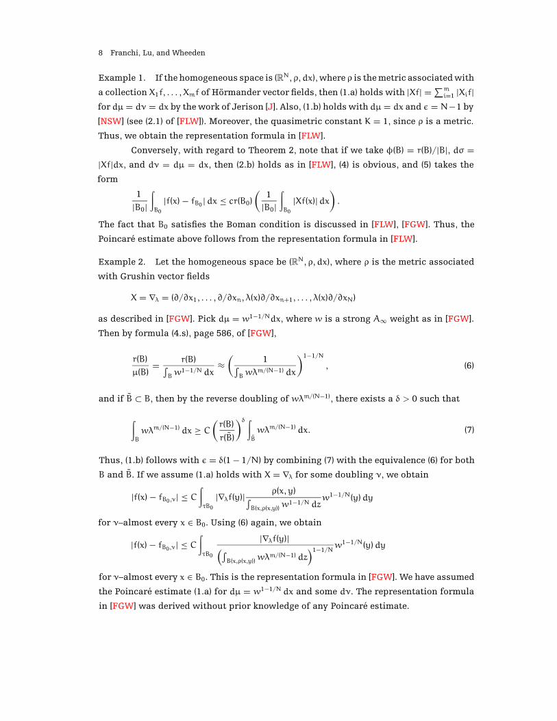
8 Franchi, Lu, and Wheeden

Example 1. If the homogeneous space is (RN, ρ, dx),where ρ is the metric associated with

a collection X1f, . . . , Xmf of Hormander vector fields, then (1.a) holds with |Xf| =∑mi=1 |Xif|

for dµ = dν = dx by the work of Jerison [J]. Also, (1.b) holds with dµ = dx and ε = N−1 by

[NSW] (see (2.1) of [FLW]). Moreover, the quasimetric constant K = 1, since ρ is a metric.

Thus, we obtain the representation formula in [FLW].

Conversely, with regard to Theorem 2, note that if we take φ(B) = r(B)/|B|, dσ =|Xf|dx, and dν = dµ = dx, then (2.b) holds as in [FLW], (4) is obvious, and (5) takes the

form

1

|B0|∫B0

|f(x)− fB0 |dx ≤ cr(B0)(

1|B0|∫B0

|Xf(x)|dx).

The fact that B0 satisfies the Boman condition is discussed in [FLW], [FGW]. Thus, the

Poincare estimate above follows from the representation formula in [FLW].

Example 2. Let the homogeneous space be (RN, ρ, dx), where ρ is the metric associated

with Grushin vector fields

X = ∇λ = (∂/∂x1, . . . , ∂/∂xn, λ(x)∂/∂xn+1, . . . , λ(x)∂/∂xN)

as described in [FGW]. Pick dµ = w1−1/Ndx, where w is a strong A∞ weight as in [FGW].

Then by formula (4.s), page 586, of [FGW],

r(B)

µ(B)= r(B)∫

Bw1−1/N dx

≈(

1∫Bwλm/(N−1) dx

)1−1/N

, (6)

and if B ⊂ B, then by the reverse doubling of wλm/(N−1), there exists a δ > 0 such that

∫B

wλm/(N−1) dx ≥ C(r(B)

r(B)

)δ ∫B

wλm/(N−1) dx. (7)

Thus, (1.b) follows with ε = δ(1− 1/N) by combining (7) with the equivalence (6) for both

B and B. If we assume (1.a) holds with X = ∇λ for some doubling ν, we obtain

|f(x)− fB0,ν| ≤ C∫τB0

|∇λf(y)| ρ(x, y)∫B(x,ρ(x,y))w

1−1/N dzw1−1/N(y)dy

for ν–almost every x ∈ B0. Using (6) again, we obtain

|f(x)− fB0,ν| ≤ C∫τB0

|∇λf(y)|(∫B(x,ρ(x,y))wλ

m/(N−1) dz)1−1/N

w1−1/N(y)dy

for ν–almost every x ∈ B0. This is the representation formula in [FGW]. We have assumed

the Poincare estimate (1.a) for dµ = w1−1/N dx and some dν. The representation formula

in [FGW] was derived without prior knowledge of any Poincare estimate.

Poincare-Type Inequalities and Representation Formulas 9

Conversely, we will show by using Theorem 2 that the representation formula

above implies (1.a) withdµ = w1−1/Ndx anddν chosen to be eitherw1−1/Ndx orwλm/(N−1)dx.

In fact, first let

dµ = w1−1/Ndx, φ(B) = r(B)

µ(B), and dσ = |∇λf|dµ.

Then, by (6), the representation formula in [FGW] for a ball B is the same as (2.a). We

will now show that (2.b) and (4) hold if dν is either dµ or wλm/(N−1)dx. The estimate (4)

is obvious if dν = dµ, while if dν = wλm/(N−1)dx, then by using (6), we see that (4) is

equivalent to

ν(B)ν(B0)

≤ c ν(B)1−1/N

ν(B0)1−1/N, B ⊂ B0,

which is obvious since ν(B) ≤ ν(B0) if B ⊂ B0.

It remains to show (2.b) for either choice of ν. Since µ is a doubling measure, we

have

φ(B(x, ρ(x, y))) ≈ φ(B(y, ρ(x, y)))

and ∫B

φ(B(x, ρ(x, y)))dν(x) ≈∫B

φ(B(y, ρ(x, y)))dν(x).

Since y ∈ τB, by enlarging the domain B of integration proportionally, we may assume

that y is the center of B. The last integral is then at most

∞∑k=0

∫{x:ρ(x,y)≈2−kr(B)}

φ(B(y, ρ(x, y)))dν(x) ≤ c∞∑k=0

φ(2−kB)ν(2−kB).

If ν = µ, this sum is

c

∞∑k=0

r(B)2−k = cr(B) = cφ(B)ν(B),

which proves (2.b). If dν = wλm/(N−1)dx, then φ(B) ≈ ν(B)1/N−1 by (6), and the sum above

is at most

c

∞∑k=0

ν(2−kB)1/N ≤ c∞∑k=0

(2−kεν(B)

)1/Nfor some ε > 0 by reverse doubling of ν, which is equal to

cν(B)1/N = cν(B)1/N−1ν(B) ≤ cφ(B)ν(B).

This proves (2.b) in every case. Finally, since balls satisfy the Boman condition by Theo-

rem 5.4 of [FGW], the representation formula in [FGW] then implies (1.a) for either choice

of ν, with dµ = w1−1/Ndx.

10 Franchi, Lu, and Wheeden

Example 3. In the general setting, if we assume that r(B)/µ(B) ≈ η(B)−α for some α > 0

and some measure η that satisfies a reverse doubling condition, then (1.b) is clearly

satisfied, and so (1.a) implies by Theorem 1 that

|f(x)− fB0,ν| ≤ C∫τKB0

|Xf(y)| ρ(x, y)

µ(B(x, ρ(x, y)))dµ(y)

for ν–almost every x ∈ B0. This example includes the class of nonsmooth vector fields

considered in [FL] and [F1] by picking dµ = dx, since we know there is a compensation

couple, i.e., a doubling measure ηdx and s > 1 such that

r(B)

|B| ≈ η(B)−1/s.

In fact, by [FW], we may choose s = N/(N− 1) and dη = (Πλj)1/(N−1)dx, where Xj = λj(x)∂j,

j = 1, . . . , N, are assumed to satisfy the conditions in [F1]. Arguing as in Example 2

with φ(B) = r(B)/|B|, dσ = (∑ |Xjf|)dx, and dµ = dx, we obtain by Theorem 2 that the

representation formula in [F2] implies (1) with dµ = dx and dν taken to be either dx or

dη. We omit the details.

Example 4. Let G be a connected Lie group endowed with its left-invariant Haar mea-

sure µ. For the sake of simplicity, let us suppose thatG is unimodular, and let {X1, . . . , Xm}be a family of left-invariant vector fields on G which generate its Lie algebra. Then we

can define a natural left-invariant metric ρ on G (see [VSC] for precise definitions) so that

there exists a positive integer d such that, for any ρ-ball B(x, r),we have that µ(B(x, r)) ≈ rdas r→ 0. If, in addition, G has polynomial growth at infinity, then there exists a nonneg-

ative integer D such that µ(B(x, r)) ≈ rD as r→∞. Thus, if we assume that min{d,D} > 1,

then (1.b) holds with ε = min{d,D} − 1 for all balls B0 ⊂ G, so that the hypotheses

of Theorem 1 are satisfied, since the Poincare inequality (1.a) with ν = µ holds by [V]

and [MS]. (The doubling property of the measure of balls follows in a straightforward

way from the existence of d and D.) Thus, a representation formula in G follows for all

balls B0.

Analogous arguments can be carried out for the balls of M = G \H, where H is a

closed subgroup of G: see again [MS, Example 4], and the literature quoted therein. For

further information on these subjects, see [VSC].

Example 5. As is well known, representation formulas like (1.c) and (1.c′), when used

in conjunction with known facts about operators of potential type, lead to two-weight

Lp, Lq Poincare inequalities, 1 ≤ p ≤ q <∞, where the Lp norm appears on the right side

of the inequality and the Lq norm on the left. We shall not explicitly recall any results of

Poincare-Type Inequalities and Representation Formulas 11

this kind here, but refer to [SW], [FGW], [FLW], [L1], [L2] and the references listed in these

papers for precise statements. In particular, it then follows from Theorem 1, by using

the representation formula, that (1.a) and (1.b) also lead to such weighted Lp, Lq Poincare

estimates.

After Saloff-Coste’s paper [Sal], many results in the same spirit (see also, e.g.,

[MS], [BM], and [HK]) have been proved in different settings, stating (roughly speaking)

that if an L1, L1 Poincare inequality like (1.a) holds with µ = ν, together with a doubling

property of the measure, then (1.a) can be improved by replacing the L1-norm on the

left side by an Lq-norm for some q > 1 depending on the doubling order. As long as the

value of q is the best possible, Poincare inequalities with p = 1 contain deep geometric

information since they imply suitable relative isoperimetric inequalities (see [FLW]). Now,

if (1.a) and (1.b) hold, then the weighted Lp, Lq Poincare inequalities which we obtain by

using the representation formula extend some of the results in the papers listed above.

The results in these papers are obtained without using a representation formula. They

include analogues when the initial Poincare hypothesis is an Lp, Lp estimate for some

p > 1, rather than just when p = 1. Many such analogues, including two-weight versions,

can also be obtained by using representation formulas which are similar to (1.c), but

which are instead based on an initial Lp, Lp Poincare hypothesis. In fact, analogues of

Theorems 1 and 2 for this situation will be discussed in a sequel to this paper.

Example 6. In [Ha], the author defines a class of first-order Sobolev spaces on a generic

metric space (S, ρ) endowed with a Borel measure µ as follows: if 1 < p ≤ ∞, then

W1,p(S, ρ, µ) denotes the set of all f ∈ Lp(S, µ) for which there exist E ⊂ S, µ(E) = 0, and

g ∈ Lp(S, µ) such that

|f(x)− f(y)| ≤ ρ(x, y)(g(x)+ g(y)

)(8)

for all x, y ∈ S\E. Sobolev spaces associated with a family of Hormander vector fields are

examples of such spaces, as well as weighted Sobolev spaces associated with a weight

function belonging to Muckenhoupt’s Ap classes. Now, it follows from our Theorem 1

that, if µ is a doubling measure such that (1.b) holds, then the pointwise condition (8) is

a corollary of the weaker integral condition

∫B

|f(y)− fB|dµ(y) ≤ Cr∫B

|g(y)|dµ(y) (9)

for all ρ-balls B = B(x, r), where g ∈ Lp(S, µ) is a given function depending on f but

independent of B. Indeed, by Theorem 1, (9) implies that for µ–almost every y ∈ B,

12 Franchi, Lu, and Wheeden

we have

|f(y)− fB,µ| ≤ C∫τB

|g(z)| ρ(y, z)

µ(B(y, ρ(y, z)))dµ(z) ≤ C

∫(τ+1)B(y,r)

|g(z)| ρ(y, z)

µ(B(y, ρ(y, z)))dµ(z)

≤0∑

k=−∞

∫2k−1(τ+1)r≤ρ(z,y)<2k(τ+1)r

|g(z)| ρ(y, z)

µ(B(y, ρ(y, z)))dµ(z)

≤ Cr0∑

k=−∞2k∫B(y,2k(τ+1)r)

|g(z)|dµ(z)

≤ CrMg(y),

whereMg denotes the Hardy-Littlewood maximal function of g with respect to the mea-

sure µ,which belongs to Lp(S, µ) if p > 1. Thus, if x, y ∈ S,we can apply the above estimate

to the ball B = B(x, 2ρ(x, y)), and we get

|f(x)− f(y)| ≤ |f(x)− fB,µ| + |f(y)− fB,µ|

≤ Cρ(x, y) {Mg(x)+Mg(y)} ,

and then (8) holds. Thus, since (8) implies (9) [Ha, Lemma 2], (9) provides us with an

alternative definition of Sobolev spaces associated with a metric.

More generally,we can easily modify the argument above to show that (9) implies

|f(x)− f(y)| ≤ C ρ(x, y)µ(B(x, ρ(x, y)))1−α

{Mαg(x)+Mαg(y)} (10)

for any α satisfying 1 − 1/d < α ≤ 1, where d is the doubling order of µ (i.e., where

µ(B(y, r)) ≤ c(r/s)dµ(B(y, s)) if s < r) and Mαg is the fractional maximal function of g

defined by

Mαg(x) = supr>0

1

µ(B(x, r))α

∫B(x,r)|g(z)|dµ(z).

Acknowledgments

The first author was partially supported by MURST, Italy (40% and 60%), and GNAFA of CNR, Italy.

The second and third authors were partially supported by NSF grants DMS93-15963 and 95-00799.

References

[BM] M. Biroli and U. Mosco, Proceedings of the Conference Potential Theory and Partial Differ-

ential Operators with Nonnegative Characteristic Form, Parma, February 1994, Kluwer,

Amsterdam, to appear.

Poincare-Type Inequalities and Representation Formulas 13

[CDG1] L. Capogna, D. Danielli, and N. Garofalo, Subelliptic mollifiers and a characterization of

Rellich and Poincare domains, Rend. Sem. Mat. Univ. Politec. Torino 54 (1993), 361–386.

[CDG2] , Subelliptic mollifiers and a basic pointwise estimate of Poincare type, preprint,

1995.

[CW] R. R. Coifman and G. Weiss, Analyse harmonique non-commutative sur certains espaces

homogenes, Lecture Notes in Math. 242, Springer-Verlag, Berlin, 1971.

[FP] C. Fefferman and D. H. Phong, “Subelliptic eigenvalue problems” in Conference on Har-

monic Analysis in Honor of Antoni Zygmond, ed. by W. Beckner et al., Wadsworth,

Belmont, Calif., 1981, 590–606.

[F1] B. Franchi, Weighted Sobolev-Poincare inequalities and pointwise estimates for a class

of degenerate elliptic equations, Trans. Amer. Math. Soc. 327 (1991), 125–158.

[F2] , Inegalites de Sobolev pour des champs de vecteurs lipschitziens, C. R. Acad. Sci.

Paris Ser. I Math. 311 (1990), 329–332.

[FGW] B. Franchi, C. Gutierrez, and R. L. Wheeden, Weighted Sobolev-Poincare inequalities for

Grushin type operators, Comm. Partial Differential Equations 19 (1994), 523–604.

[FL] B. Franchi and E. Lanconelli,Holder regularity theorem for a class of linear nonuniformly

elliptic operators with measurable coefficients, Ann. Scuola Norm. Sup. Pisa Cl. Sci. (4) 10

(1983), 523–541.

[FLW] B. Franchi, G. Lu, and R. L. Wheeden, Representation formulas and weighted Poincare

inequalities for Hormander vector fields, Ann. Inst. Fourier (Grenoble) 45 (1995), 577–604.

[FW] B. Franchi and R. L. Wheeden, Compensation couples and isoperimetric estimates for

vector fields, preprint, 1995.

[Ha] P. Hajlasz, Sobolev spaces on an arbitrary metric space, Potential Anal., to appear.

[HK] P. Hajlasz and P. Koskela, Sobolev meets Poincare, C. R. Acad. Sci. Paris Ser. I Math. 320

(1995), 1211–1215.

[H] L. Hormander, Hypoelliptic second order differential equations, Acta Math. 119 (1967),

147–171.

[J] D. Jerison, The Poincare inequality for vector fields satisfying Hormander’s condition,

Duke Math. J. 53 (1986), 503–523.

[LW] E. P. Lotkowski and R. L. Wheeden, The equivalence of various Lipschitz conditions on

the weighted mean oscillation of a function, Proc. Amer. Math. Soc. 61 (1976), 323–328.

[L1] G. Lu, Weighted Poincare and Sobolev inequalities for vector fields satisfying Horman-

der’s condition and applications, Rev. Mat. Iberoamericana 8 (1992), 367–439.

[L2] , The sharp Poincare inequality for free vector fields: an endpoint result, Rev. Mat.

Iberoamericana 10 (1994), 453–466.

[MS] P. Maheux and L. Saloff-Coste, Analyse sur les boules d’un operateur sous-elliptique, to

appear in Math. Ann.

[NSW] A. Nagel, E. M. Stein, and S. Wainger, Balls and metrics defined by vector fields I: basic

properties, Acta Math. 155 (1985), 103–147.

[RS] L. P. Rothschild and E. M. Stein, Hypoelliptic differential operators and nilpotent groups,

Acta Math. 137 (1976), 247–320.

[Sal] L. Saloff-Coste, A note on Poincare, Sobolev and Harnack inequalities, Internat. Math.

14 Franchi, Lu, and Wheeden

Res. Notices 1992, 27–38.

[San] A. Sanchez-Calle, Fundamental solutions and geometry of the sums of squares of vector

fields, Invent. Math. 78 (1984), 143–160.

[SW] E. Sawyer and R. L. Wheeden,Weighted inequalities for fractional integrals on Euclidean

and homogeneous spaces, Amer. J. Math. 114 (1992), 813–874.

[V] N. Varopoulos, Fonctions harmoniques sur les groupes de Lie, C. R. Acad. Sci. Paris Ser. I

Math. 304 (1987), 519–521.

[VSC] N. Varopoulos, L. Saloff-Coste, and T. Coulhon, Analysis and Geometry on Groups, Cam-

bridge Univ. Press, Cambridge, 1992.

Franchi: Dipartimento di Matematica, Universita di Bologna, Piazza di Porta S. Donato, 5, I40127,

Bologna, Italy; franchib@dm.unibo.it

Lu: Department of Mathematics, Wright State University, Dayton, Ohio 45435, USA;

gzlu@euler.math.wright.edu

Wheeden: Department of Mathematics, Rutgers University, New Brunswick, New Jersey 08903,

USA; wheeden@math.rutgers.edu