Analisi Numerica: Metodi e Software Matematico

Progetto cofinanziato dal MURST - 1998–2000

A Random Generator for Large–ScaleLinearly Constrained QuadraticProgramming Test Problems

C. Durazzi V. Ruggiero

Dipartimento di MatematicaUniversita di Ferrara

L. Zanni

Dipartimento di MatematicaUniversita di Modena e Reggio Emilia

Monografia n. 6

Ferrara 2000

Monografie del Programma di Ricerca Scientifica 1998–2000“Analisi Numerica: Metodi e Software Matematico”

cofinanziato dal Ministero per l’Universita ela Ricerca Scientifica e Tecnologica nell’anno 1997.

Monographs of the 1998–2000 Scientific Research Program“Numerical Analysis: Methods and Mathematical Software”supported in 1997 by the Italian Ministry for the University

and the Scientific and Technological Research.

http://www.unife.it/AnNum97

Abstract

In this paper we describe a random generator for large and sparse quadratic programmingproblems that frequently arise in different areas of applied science. This generator is anuseful tool in testing algorithms on QP problems with different features, since it allowsus to vary many parameters which characterize the problems.The procedure used to generate a QP problem as well as some details for its implemen-tation are explained.Finally, we report an analysis of the numerical results, obtained by the routine E04NFKof the NAG library on the test problems produced by the generator.

C. Durazzi V. Ruggiero

Dipartimento di Matematica, Universita di Ferrara, Via Machiavelli 35, Ferrara, Italy.E-mail: {dzc,rgv}@dns.unife.it.L. Zanni

Dipartimento di Matematica, Universita di Modena e Reggio Emilia, Via Campi 213/b, 41100Modena, Italy. E-mail: zanniluca@unimo.it.

a random generator for quadratic programming test problems

Contents

Contents i

1 Introduction 1

2 A procedure for randomly generating a QP problem 3

3 Implementation of the test problem generator 7

4 Numerical evaluation of the routine E04NKF 11

Bibliography 15

a random generator for quadratic programming test problems

Chapter 1

Introduction

In many areas of science and technology it is required to solve the following linearlyconstrained quadratic programming (QP) problem

minimize f(x) = 12xT Gx + qT x

subject to Cx = d, Ax ≥ b,(1.1)

where G is a symmetric matrix of order n, C is an me×n matrix of full row rank (me ≤ n)and A is an mi × n matrix.At the moment, attention is greatly focused on large QP problems where G, C and Amay be sparse matrices, without a particular structure. These large problems are basicto many applications of data analysis, such as image restoration [1], pattern recognitionbased upon support vector machine technique [3] and constrained bivariate interpolation[5]. Furthermore, large QP problems arise as subproblems of the class of symmetriccost approximation methods [13] for large–scale nonlinear programming or variationalinequality problems when the auxiliary function is a convex quadratic function or thegradient map of a convex quadratic function. See, for example, the sequential quadraticprogramming method or, for the variational inequalities, the linear approximation meth-ods [12] and the descent methods based upon projective gap functions [14].In order to make clear the “effectiveness” of the solvers proposed in literature for largeQP problems, it is necessary to evaluate the numerical behaviour of these methods byan extensive experimentation on vaste sets of test problems with different features.Well–known collections of QP problems of the form (1.1) are contained in CUTE [2](http://www.cse.clrc.ac.uk/Activity/CUTE) and in the repository at the URLhttp://www.doc.ic.ac.uk/∼im/#DATA [9] (see also the following URL for a list of test-cases in optimization: http://plato.la.asu.edu/topics/testcases.html).The aim of this work is to describe a generator for random, large and sparse quadraticprograms. This generator enables us to prefix the most part of the parameters thatcharacterize a problem and, above all, it permits to specify the distribution of the singularvalues of the matrices of the constraints and the spectrum of the hessian and the reducedhessian of the objective function. Thus we can generate poorly or well–conditionedproblems of arbitrary size, number of constraints and level of sparsity. Varying in aconvenient way the parameters which the test problems depend on, we can reflect thefeatures of the quadratic programs arising in many practical applications.In Chapter 2, we describe the technique for randomly generating QP problems withassigned features. In Chapter 3, we report the way of storing the sparse matrices of theQP problem and some details of the implementation of the generator. In Chapter 4, weconsider a set of test problems produced by this generator and we show some numerical

2 Introduction

results obtained by solving the test problems with the routine E04NKF of the NAGlibrary [11].

a random generator for quadratic programming test problems

Chapter 2

A procedure for randomlygenerating a QP problem

We assume that the following data are given:

• the sparsity of the n×n matrix G (spars(G)) and of the m×n matrix B (spars(B)),

where B =(

CA

)denotes the constraint matrix (m = mi + me); furthermore we

set f =(

db

);

• the rank r(G), the spectral condition number K(G) and the maximum and theminimum nonzero eigenvalues, denoted by φmax(G) and φmin(G), of the Hessianmatrix G of (1.1); for convex QP problems, the maximum eigenvalue of G is ob-tained by φmax(G) = K(G)φmin(G);

• the spectral condition number K(B) and the minimum nonzero singular valueσmin(B) of the matrix B; the rank of B is chosen equal to min(m,n) and themaximum singular value of B is σmax(B) = K(B)σmin(B);

• a solution x∗ of (1.1), with entries xi randomly generated from an uniform distri-bution in (−1, 1);

• the number ma of the inequality constraints that are active in x∗; we denote bynac the value ma + me, so that nac ≥ me;

• an m-vector(

µ∗

λ∗

)of the multipliers associated to x∗, with null elements for the

entries corresponding to the inactive inequality constraints in x∗, µ∗i = 10−zi·ndeg

for the indices corresponding to the equality constraints and λ∗i = 10−zi·ndeg for

the indices corresponding to the active inequality constraints; here zi is randomlygenerated in (0, 1) and ndeg is an integer parameter which specifies the level ofdegeneracy;

• the rank r(ZT GZ) and the spectral condition number K(ZT GZ) of the reducedHessian ZT GZ, where Z is chosen as an orthogonal basis of the null space of thematrix given by the equality constraints and the inequality constraints active inx∗.

4 A procedure for randomly generating a QP problem

The matrix G of (1.1) is generated by its spectral decomposition

G = V DV T = V

(D1 00 D2

)V T(2.1)

where D is a diagonal matrix with maximum and minimum nonzero eigenvalues φmax(G)and φmin(G) respectively, and r(G)−2 diagonal entries randomly generated in (φmin(G),φmax(G)); in particular, the diagonal submatrix D2 of order n−nac has r(ZT GZ) positivediagonal entries chosen so that the condition number of D2 is K(ZT GZ).The matrix V is an orthogonal matrix obtained as product of a number of random Givensrotations Rij such that the matrix G is filled until the prefixed level of sparsity is attained.A random Givens rotation Rij is obtained by randomly generating two different positiveintegers i and j in the interval [1, n]. Then we randomly generate a real number α in the

interval [−1, 1] and we set α = rj,j = ri,i = cos(θ); consequently, ri,j = −rj,i =√

1 − r2i,i.

Now, we partition the matrix V in(

V1 V2

), where V1 and V2 represent the first nac

and the last n − nac columns of V respectively.

In order to generate the matrix of constraints B, we construct the m×n matrix(

BB

),

where B is the nac × n matrix of the equality constraints and the active inequalityconstraints in x∗, and B is the (m − nac) × n matrix composed by the remaining rows

of B. We write(

BB

)as follows:

B =(

BB

)=

(U1 00 U2

)(S1 00 S2

)(V T

1

V T2

)=

(U1S1V

T1

U2S2VT2

)(2.2)

where S1 is a diagonal matrix of order nac with prefixed condition number K(B) and nacpositive diagonal entries included in [σmin(B), σmax(B)]; S2 is an (m− nac)× (n− nac)matrix with min(m,n)−nac positive diagonal entries randomly generated and such that

the condition number of(

BB

)is still K(B). The rank of

(BB

)is min(m,n).

The matrices U1 and U2 are orthogonal matrices of order nac and m − nac respectively,generated as product of random Givens rotations, so that we achieve the prefixed level

of sparsity for B in the matrix(

BB

).

From (2.2) we deduce that V2 represents an orthonormal basis for the null space of B:

BV2 = U1S1VT1 V2 = 0

Thus, if we put Z = V2, from the following relation

V T2 GV2 = V T

2 ( V1 V2 )(

D1 00 D2

) (V T

1

V T2

)

= V T2 (V1D1V

T1 + V2D2V

T2 )V2 = D2

we have that the reduced Hessian has rank r(ZT GZ) and condition number K(ZT GZ),as prefixed.Then, we put

f =(

BB

)x∗ −

(0ε

)

A procedure for randomly generating a QP problem 5

where ε is a vector with positive random elements.Finally, we obtain the n-vector q of the objective function in (1.1) from the Kuhn Tuckerconditions:

q = −Gx∗ + AT λ∗ + CT µ∗.

6 A procedure for randomly generating a QP problem

a random generator for quadratic programming test problems

Chapter 3

Implementation of the testproblem generator

A random test problem generator for large–scale sparse linearly constrained convex QPproblems, based on the technique described in the previous Chapter, is written in Fortran77.The source program, contained in the file test98.f, is available at the following URL:http://www.unife.it/AnNum97/index2.htm.An exhaustive documentation, about the input data that the user has to supply andabout the output files produced by the program, is reported in the comments of thesource file. At the same URL, it is possible to get a file containing an example of theinput data (inputtest98) and a file showing the messages produced by the program(outputtest98).In the following, we explain some details of the implementation of the test problemgenerator.The nonzero eigenvalues of G and the nonzero singular values of B can be randomlygenerated in a convenient interval, according to a log–uniform distribution or an uniformdistribution or they can be equally spaced between the extrema of the interval in ques-tion. If the input variable indg (or indb for the matrix B) is equal to 0, a log–uniformdistribution for randomly generating the eigenvalues of G (or the singular values of B) isused; if indg = 1 (indb = 1, respectively) an uniform distribution is used; otherwise, theeigenvalues of G (or the singular values of B) are equally spaced between the smallestand the largest eigenvalues (or singular values). For the matrices G and B, the userhas to supply condg = log10(K(G)), condb = log10(K(B)), condzgz = log10(ZT GZ)(≤ condg) and condba = log10(B) (≤ condb). Furthermore, the following data have tobe introduced:

• for the matrix G, the minimum positive eigenvalue glmin and the rank ngrango (Gis a positive semidefinite matrix); the maximum eigenvalue of G is 10condg · glmin;

• for the matrix ZT GZ, the minimum positive eigenvalue zgzlmin (≥ glmin) andthe rank nzgzrango (≤ ngrango − nac); the maximum eigenvalue of ZT GZ is10condzgz · zgzlmin;

• the minimum nonzero singular value blmin of the matrix B; the rank of B ismin(m,n);

• the minimum nonzero singular value balmin (≥ blmin) of the matrix B; the rankof B is nac.

8 Implementation of the test problem generator

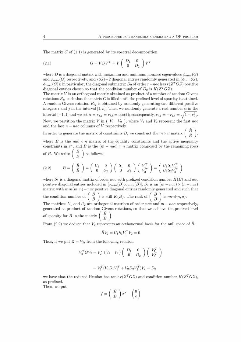
Figure 3.1: Matrix G with a band structure (n = 2000, spars(G)=99.8%).

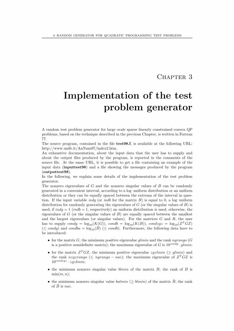
Figure 3.2: Matrix B with a band structure (m = 1000, spars(B)=99.8%).

Furthermore, the user has to supply the level of sparsity of G and B. We can alsogenerate band matrices with a prefixed bandwidth (see Figures 1–2).Finally, we describe the technique used for storing the sparse matrices G and B. Eachmatrix is stored in compressed form [8]. If we denote by kmax the largest number ofnonzero elements per row of a generic sparse nr×nc matrix A, the storage of A is madein two nr × kmax matrices AS and IAS as follows:

AS(i, 1) = A(i, i) IAS(i, 1) = i

AS(i, j) = A(i, k) and IAS(i, j) = k if A(i, k) �= 0

An nr vector KAS contains, in the i–th element, the number of nonzero entries of thei-th row of A. For example, when the matrix G is defined as

G =

3 0 2

0 4 12 1 4

(3.1)

the compressed form is given by

GS =

3 2

4 14 2 1

, KGS =

2

23

and IGS =

1 3

2 33 1 2

(3.2)

The program test98.f produces two unformatted files, containing the information aboutthe objective function and the constraints respectively. The nonzero elements of theupper triangular part of the matrix G are stored in a set of consecutive records of thefirst file, following a row wise ordering; each record contains the row index, the columnindex and the value of four nonzero elements of G. For example, the matrix G of (3.1)–(3.2) is stored in the first file as:

1 1 3 1 3 2 2 2 4 2 3 1 first record3 3 4 second record.

Implementation of the test problem generator 9

Figure 3.3: Matrix G without structure (n = 2000, spars(G)=99.9%).

Figure 3.4: Matrix B without structure (m = 1000, spars(B)=99.9%).

All the nonzero entries of the matrix B are stored in a set of consecutive records of thesecond file with the same format used for G in the first file.

10 Implementation of the test problem generator

a random generator for quadratic programming test problems

Chapter 4

Numerical evaluation of theroutine E04NKF

In this Chapter we report the numerical results obtained by the routine E04NKF of theNAG library [11] on a set of test problems generated by the technique described in theprevious Chapters. All the experiments are carried out on a Digital Alpha 500/333 Mhzworkstation, using the double precision (macheps= 2.22 · 10−16) and a Fortran program,named test nag.f, available at the URL: http://www.unife.it/AnNum97/index2.htm.This program reads the two unformatted files produced by test98.f and rearranges thedata according to the format required by E04NKF; then, this routine is called and itsresults are written in the file nag.dat.The routine E04NKF is designed to solve large–scale linear and quadratic problems withthe following constraints:

l ≤{

xFx

}≤ u

where F is a sparse m × n matrix. In the experiments reported in this Chapter, weconsider convex quadratic problems of the form (1.1), where simple box constraints arenot present and we have only general constraints (F = B). In this case, the user has toprovide a subroutine that computes the matrix–vector product Gx for any given vectorx.The routine E04NKF is based on an active–set method. This is an iterative procedurewith two phases: a feasibility phase, in which the sum of infeasibilities is minimized tofind a feasible point [4, p. 166] and an optimality phase in which f(x) is minimized byconstructing a sequence of iterations that lies within the feasible region; each iterationrequires to solve a QP problem with equality constraints only [4, p. 240]. E04NKF isbased on SQOPT, which is part of the SNOPT package [6], that in turn utilizes routinesfrom the MINOS package [10]. It uses stable numerical methods throughout and includesa reliable basis package for maintaining sparse LU factors of a convenient submatrix ofthe constraint matrix [7].In the following Tables, time denotes the elapsed time in seconds to execute E04NKF,using default setting for all the optional parameters of the routine. The values erx anderf denote the relative errors of the computed minimum point ‖x∗ − x‖2/‖x∗‖2 and ofthe minimum value of the objective function |f(x∗) − f(x)|/|f(x∗)| respectively. Herex is the approximate solution obtained by E04NKF and x∗ is the prefixed solution ofthe test problem. When rank(G) < n, the minimum point is not necessarily unique anderx is not meaningful. In all the test problems the eigenvalues of the matrix G or thesingular values of matrix B are uniformly distributed.

12 Numerical evaluation of the routine E04NKF

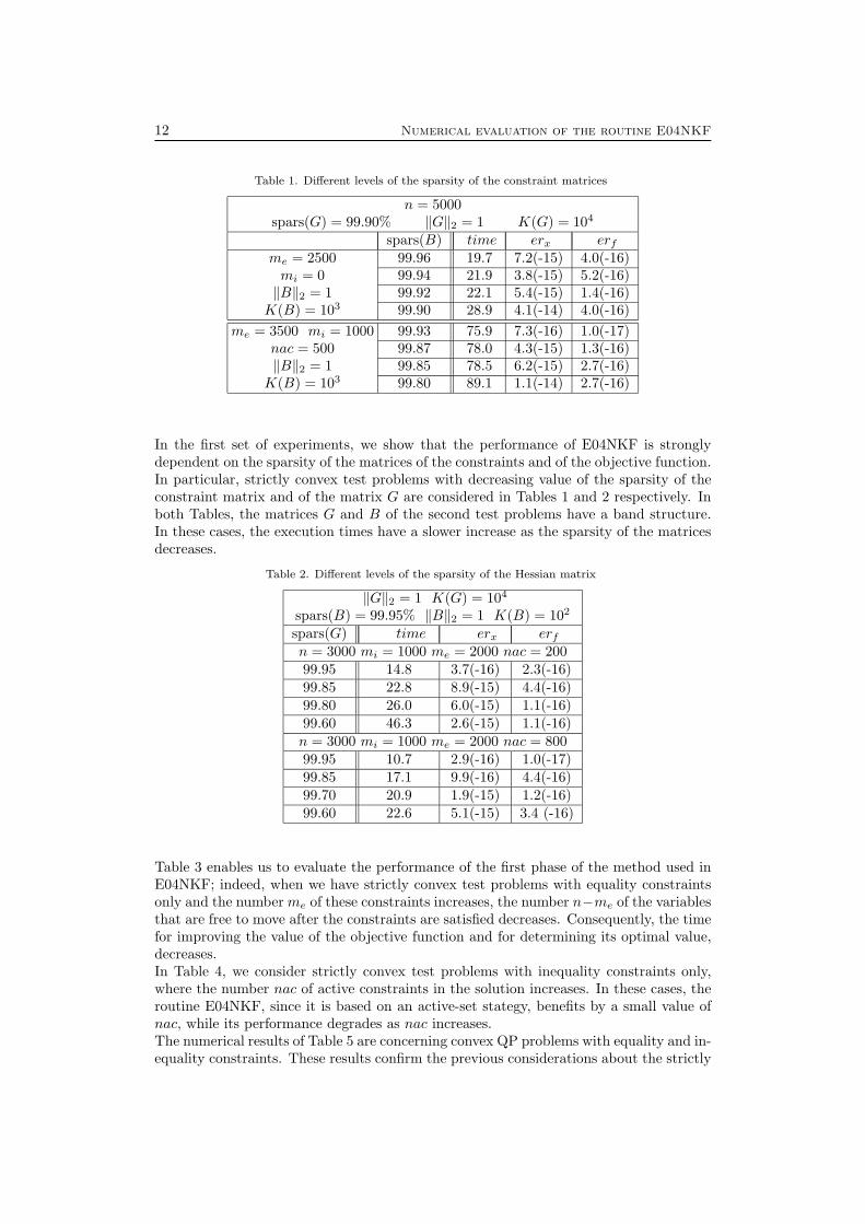
Table 1. Different levels of the sparsity of the constraint matrices

n = 5000spars(G) = 99.90% ‖G‖2 = 1 K(G) = 104

spars(B) time erx erf

me = 2500 99.96 19.7 7.2(-15) 4.0(-16)mi = 0 99.94 21.9 3.8(-15) 5.2(-16)

‖B‖2 = 1 99.92 22.1 5.4(-15) 1.4(-16)K(B) = 103 99.90 28.9 4.1(-14) 4.0(-16)

me = 3500 mi = 1000 99.93 75.9 7.3(-16) 1.0(-17)nac = 500 99.87 78.0 4.3(-15) 1.3(-16)‖B‖2 = 1 99.85 78.5 6.2(-15) 2.7(-16)

K(B) = 103 99.80 89.1 1.1(-14) 2.7(-16)

In the first set of experiments, we show that the performance of E04NKF is stronglydependent on the sparsity of the matrices of the constraints and of the objective function.In particular, strictly convex test problems with decreasing value of the sparsity of theconstraint matrix and of the matrix G are considered in Tables 1 and 2 respectively. Inboth Tables, the matrices G and B of the second test problems have a band structure.In these cases, the execution times have a slower increase as the sparsity of the matricesdecreases.

Table 2. Different levels of the sparsity of the Hessian matrix

‖G‖2 = 1 K(G) = 104

spars(B) = 99.95% ‖B‖2 = 1 K(B) = 102

spars(G) time erx erf

n = 3000 mi = 1000 me = 2000 nac = 20099.95 14.8 3.7(-16) 2.3(-16)99.85 22.8 8.9(-15) 4.4(-16)99.80 26.0 6.0(-15) 1.1(-16)99.60 46.3 2.6(-15) 1.1(-16)n = 3000 mi = 1000 me = 2000 nac = 80099.95 10.7 2.9(-16) 1.0(-17)99.85 17.1 9.9(-16) 4.4(-16)99.70 20.9 1.9(-15) 1.2(-16)99.60 22.6 5.1(-15) 3.4 (-16)

Table 3 enables us to evaluate the performance of the first phase of the method used inE04NKF; indeed, when we have strictly convex test problems with equality constraintsonly and the number me of these constraints increases, the number n−me of the variablesthat are free to move after the constraints are satisfied decreases. Consequently, the timefor improving the value of the objective function and for determining its optimal value,decreases.In Table 4, we consider strictly convex test problems with inequality constraints only,where the number nac of active constraints in the solution increases. In these cases, theroutine E04NKF, since it is based on an active-set stategy, benefits by a small value ofnac, while its performance degrades as nac increases.The numerical results of Table 5 are concerning convex QP problems with equality and in-equality constraints. These results confirm the previous considerations about the strictly

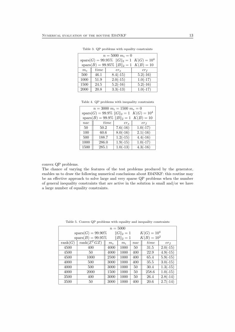
Numerical evaluation of the routine E04NKF 13

Table 3. QP problems with equality constraints

n = 5000 mi = 0spars(G) = 99.95% ‖G‖2 = 1 K(G) = 104

spars(B) = 99.95% ‖B‖2 = 1 K(B) = 10me time erx erf

500 46.1 8.4(-15) 5.2(-16)1000 51.9 2.0(-15) 1.0(-17)1500 24.5 5.2(-16) 5.2(-16)2000 20.8 3.3(-13) 1.0(-17)

Table 4. QP problems with inequality constraints

n = 3000 mi = 1500 me = 0spars(G) = 99.9% ‖G‖2 = 1 K(G) = 104

spars(B) = 99.9% ‖B‖2 = 1 K(B) = 10nac time erx erf

50 50.2 7.6(-16) 1.0(-17)100 60.6 8.0(-16) 2.1(-16)500 188.7 1.2(-15) 4.4(-16)1000 286.0 1.9(-15) 1.0(-17)1500 285.1 1.0(-13) 4.3(-16)

convex QP problems.The chance of varying the features of the test problems produced by the generator,enables us to draw the following numerical conclusions about E04NKF: this routine maybe an effective approach to solve large and very sparse QP problems when the numberof general inequality constraints that are active in the solution is small and/or we havea large number of equality constraints.

Table 5. Convex QP problems with equality and inequality constraints

n = 5000spars(G) = 99.90% ‖G‖2 = 1 K(G) = 104

spars(B) = 99.95% ‖B‖2 = 1 K(B) = 102

rank(G) rank(ZT GZ) me mi nac time erf

4500 400 4000 1000 50 31.5 2.0(-15)4500 50 4000 1000 400 22.9 4.9(-15)4500 1000 2500 1000 400 65.4 5.9(-15)4000 500 3000 1000 400 35.5 3.0(-15)4000 500 3000 1000 50 30.4 1.3(-15)4000 2000 1500 1000 50 258.6 1.0(-15)3500 400 3000 1000 50 26.4 2.8(-14)3500 50 3000 1000 400 20.6 2.7(-14)

14 Numerical evaluation of the routine E04NKF

a random generator for quadratic programming test problems

Bibliography

[1] H. C. Andrews - B. R. Hunt, Digital Image Restoration, Prentice Hall, EnglewoodPress, New Jersey, (1977).

[2] I. Bongartz - A. R. Conn - N. Gould - Ph. L. Toint, CUTE: constrained andunconstrained testing environment, ACM Transaction on Mathematical Software, 21,(1995), pp. 123–160.

[3] C. Cortes - V. N. Vapnik, Support vector network, Machine Learning, 20, pp.1–25 (1995).

[4] R. Fletcher, Practical Methods od Optimization, Second Edition, John Wiley &Son Ltd., (1987).

[5] E. Galligani, C1 surface interpolation with constraints, Numerical Algorithms, 5,(1993), pp. 549–555.

[6] P. E. Gill - W. Murray - M. A. Saunders, SNOPT: An SQP Algorithm forLarge–Scale Constrained Optimization, Numerical Analysis Report 96-2, Departe-ment of Mathematics, University of California, San Diego, (1996).

[7] P. E. Gill - W. Murray - M. A. Saunders - M. H. Wright, Maintaining LUFactors of a General Sparse Matrix, Linear Algebra and its Applics., 88/89, (1987),pp. 239–270.

[8] D. R. Kinkaid - T. C. Oppe - J. R. Respess - D. M. Young, ITPACKV2 2CUser’s Guide, Report CNA–191, Centre for Numerical Analysis, University of Texas,Austin, (1984).

[9] I. Maros - Cs. Meszaros, A Repository of Convex Quadratic Programming Prob-lems, Optimization Methods and Software, (1999).

[10] B. A. Murtagh - M. A. Saunders, MINOS 5.4, User’s Guide, Report SOL83-20R, Department of Operations Research, Stanford University, (1995).

[11] NAG Fortran Library Manual, Mark 18, (1998).

[12] J. S. Pang - D. Chan, Iterative methods for variational and complementarityproblems, Mathematical Programming, 24, (1982), pp. 284–313.

[13] M. Patriksson, Nonlinear Programming and Variational Inequality Problems: AUnified Approach, Kluwer Academic Publisher, Dordrecht, (1999).

[14] D. L. Zhu - P. Marcotte, An extended descent framework for variational inequal-ities, Journal of Optimization Theory and Applications, 80, (1994), pp. 349–366.