a qualitative ecological model to support mariculture pond water quality management

CABIOS Vol. 11 no. 6 1995Pages 595-602

A qualitative ecological model to supportmariculture pond water quality management

D.J.H.Brown

Abstract

A qualitative model of the ecology of a mariculture pond isdescribed. The model represents ecological relationships inthe form of a network of tableaux of inference rules whichare scanned by a deductive reasoning mechanism to computethe values of pond water quality indicators, make forecastsand determine appropriate corrective and/or preventativemaintenance actions.

Introduction

Artificial environments such as mariculture ponds provideuseful mesocosms within which to explore ecologicaltheories and models. The survival and growth of theorganisms being cultured depends upon the physical andchemical characteristics of the pond (Piedahitra, 1988),which may collectively be termed the 'pond water quality'.

A number of quantitative sumulation models ofaquaculture ponds have been developed which focus onmass and/or energy balances. According to Piedahitra(1986), 'these models are site-specific and of rather limitedgeneral use'. A qualitative modelling approach may besuitable for modelling water quality determinants for thefollowing reasons:

• The principles of quality control (Ishikawa, 1985)involve assigning qualitative values to the quantitativedata that characterize a situation (such as 'withincontrol limits', 'high', 'increasing', etc.) and reasoningabout the situation in terms of the qualified data todetermine maintenance actions that would preventadverse conditions persisting.

• Instrumentation of the pond is limited because ofcost/benefit considerations and many importantobservations (such as the density of the phyto-plankton bloom and the colour of the water) arereadily made in qualitative terms by a mariculturalist.

Representation of causal relationships

The qualitative model described here takes the form of aset of parameters and a network of causal relationshipsbetween them, an overview of which is shown in Figure 1.

College of Computer Studies, De La Salle University. Manila, Philippines

The model reflects practices at the Mariculture Researchand Training Centre at the University of CentralQueensland, Australia for the cultivation of Penaeusmonodon (Davis, 1992). The parameters of the model arewater quality indicators and control action recommenda-tions. Each node of the network is a computationalrepresentation of a causal relationship. For example, thenode salinity.tx computes values of the indicator 'forecastsalinity' and the recommendation 'water exchange' fromthe values of'salinity' and 'salinity trend'.

A common way of representing causal relationships incomputational models is as a set of inference rules. Themodel described here is implemented in Tableaux (Brown,1988), a logic representation scheme similar to decisiontables, in which inference rules that have commonparameters may be grouped together. {Tableaux doesnot distinguish between parameters that denote physicalproperties of a system being modelled and parameters thatdenote control actions.) Parameter values in Tableauxmay be quantitative or qualitative. A qualitative value is aset of quality classes. [Qualitative values in Tableaux arenon-deterministic. A value such as {'low, normal'}signifies a value that is 'low' or 'normal' or both (qualityclasses are not necessarily disjoint).] A Tableaux ruleantecedent is a logical conjunction of criteria. A criterionis a set of quality classes. A parameter matches a criterionif its value has a non-null intersection with the criterion. Ifthe antecedent of a rule is matched, the inferences of itsconsequent are made. [Making an inference involvessupplementing (but not replacing) the designated para-meter's value with the value specified in the ruleconsequent.]

The Tableaux Matcher (Orenstein, 1988) makes infer-ences by applying the rules in a tableau. Values ofantecedent parameters are obtained by 'backward chain-ing' (Hayes-Roth et al., 1983), which involves tracing backalong the network of causal relationships in the networkto perform computations. A simulation run of the model isperformed by applying the Matcher to the ultimate link inits causal chain, the tableau growth.tx (Figure 2), whichcomputes the value of 'forecast growth rate' (unlesspreventative maintenance action is taken) from the valuesof'forecast temperature', 'forecast pH", 'forecast oxygena-tion', 'forecast salinity' and 'prawn health'. Temperature

© Oxford University Press 595

at Mem

orial University of N

ewfoundland on A

ugust 2, 2014http://bioinform

atics.oxfordjournals.org/D

ownloaded from

http://bioinformatics.oxfordjournals.org/

D.J.H.Brown

penetration

algal bloom^ ^ growth

phottayiLtz

zooplanktongrowth

pbytcaus.tx

futureoxygenation

femlner

stocking rate

feed tray appetite / futureconsumption I ^ / temperature

ammonia production

average temperature

ammooia.tx

temperature \ pH trendtempenLtx ^ — trend

salinitytalinity ** wcatbcr.txtrend

lime

ndinity.bt sunshine forecast \

pH.U

future growthand lurvival

rainfall forecast

future pH level

Fig. 1. Structure of the model.

and salinity, while causing independent responses, arenoted by Venkataramaih et al. (1972) to have combinedeffects on prawn growth and survival rates. At normaltemperatures, growth and survival are consistent acrosswide salinity ranges (rule 1). Similarly, they are alsoconsistent over a wide temperature range in media of lowsalinity (rule 2). Abnormal pH and lack of oxygenationhave deleterious effects (rules 4 and 5). Preventativemaintenance action recommendations to forestall adverseconditions are made in the course of computing the valuesof the forecasts, as will be seen in the next section.

On the display, the horizontal gap separates antecen-dent parameters from consequent parameters. A nullcriterion (displayed as a blank cell) is satisfied by any

value. A null inference (also displayed as a blank cell)means nothing is inferred. The tilde (~) denotes logicalnegation. For example, Rule 3 may be read as:

If 'forecast temperature' is not 'normal' and 'forecastsalinity' is 'high'Then 'forecast growth rate' is 'below target'

The tableau is displayed in 'compact' format, whereinidentical criteria in adjacent rules are not replicated on thedisplay; for example, rules 1 and 2 each have the criterion:'forecast oxygenation' is not 'low [Rule names ('rule 1','rule 2', etc.) are for identification purposes only, althoughdisplaying them in different orders can reveal differentgroupings to the eye.]

5%

at Mem


ewfoundland on A



ownloaded from


A qualitative ecological model to support mariculture pond water quality management

file £dit Options Utility Check Inference

forecast_temaerature

forecast«*|]nifu

forecast pH

forecast

prawn health

orecast growthrate

Rule!

normal

Rule 2

low

normal

~low

good

on target

Rule 3

"normal

high

Rule 4 Rule 5

low

'normal

below target

Fig. 2. growth.tx.

Case study

The use of the model to determine recommendedpreventative maintenance actions is illustrated in thecontext of a case study, for which values of observationsare given in Table 1. The scenario is a situation that is nottoo serious at the moment, but conditions are such that itcould become so unless preventative maintenance action istaken.

Dissolved oxygen is generally accepted to be the mostimportant factor limiting aquaculture production inponds (Boyd, 1982). The major sources of dissolvedoxygen in the pond water are photosynthetic processesand diffusion from the atmosphere. Figure 3 displays thetableau oxysol.tx which contains rules that determines thevalue of 'forecast oxygenation' and infers appropriatepreventative maintenance actions. For example, a trendtoward a potential oxygenation crash prompts a recom-mendation to take emergency action (rules 1, 2); a

Table I. Observed values in water quality indicators

Parameter Value

Time of dayPrawn healthDissolved oxygenWater temperatureSalinitypHSecchi disc depthRecent change in secchi depthAlgal bloomColour of waterLablab depth"Forecast sunshineForecast rainfallWater exchange rateFeed tray feed consumption rateStocking densityPhase of the moon

dawngood2.9 p.p.m27°C28p.pt.923 cmnonethinbrownlittlehighnoneusuallowlownew

File Edit Options Utility Check Inference

Rule 1

Rule?

Rule 3

Rule *

Rule 7

RuleS

Rule 6

oxygentrend

decreasing,steady

decreasing

Increasing

steady

decreasing

increasing

oxygenation

crash

low

crash

low

ok

low

forecastoxygenation

crash

low

ok

low

ok

waterexchange

SOX

33%

33*

aeration

increase

Increase

•EL

Fig. 3. oxysol.tx.

predicted less serious deficiency prompts moderateremedial action (rules 4 and 5).

The value of the parameter 'oxygenation' is computedby oxylevel.tx (Figure 4). Dissolved oxygen follows adiurnal cycle; it is consumed at a fairly even rate byrespiration processes, but increases during daylight hoursfrom photosynthesis by the phytoplankton bloom. 'Low'and 'crash' oxygenation levels at dusk cannot bereplenished overnight with consequent health risks to theprawns, thereby necessitating remedial action (rules 3, 4and 5) or emergency action (rules 1 and 2), depending onthe seriousness of the situation. The model assumes that10% water exchanges are made continuously, followingpractices at the University of Central QueenslandMariculture Research and Training Centre farm (Davis,1992), with larger volume exchanges being made wheneverexceptional circumstances arise.

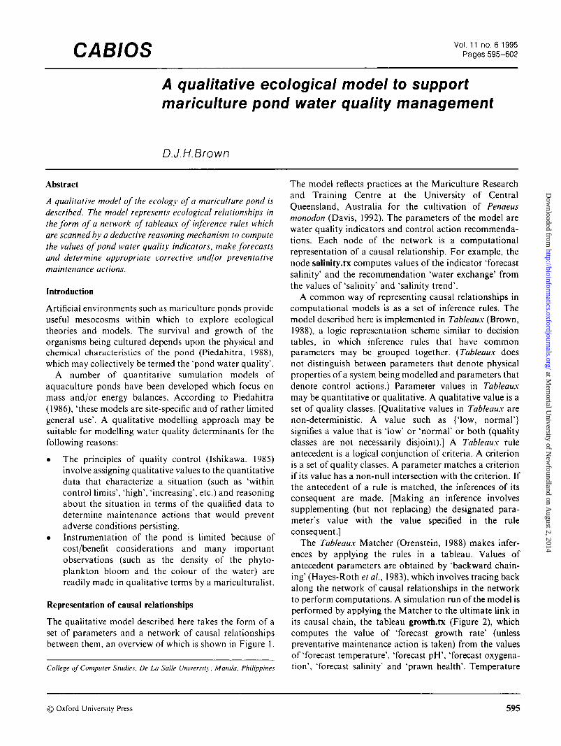
In the scenario, 'dissolved oxygen' (2.9 p.p.m.) isclassified by oxylevel.tx as 'low'. This, together with thevalue 'dawn' of the parameter 'time of day', satisfies theantecedent of rule 2, which assigns the value 'ok' to'oxygenation'. The tableau oxygen.tx (Figure 5) maps'oxygen production' and 'oxygen demand' onto 'oxygentrend'. In the scenario (as will be seen later) the Matcherestablishes 'oxygen production' is 'low' and 'oxygen

file Edit Options Utility Check Inference

° Lablab is a Filipino term for the black sludge at the bottom of pondscomposed of decaying organic matter.

dissolvedoxygen

time of day

oxygenation

exchange

aeration

food supply

Rule 1

<=

dawn

low

33X

Increase

Rule 4

dusk

crash

SOX

emergency

reduce

RuleS

>2«<S

lOW

3 3 *

ncrease

Rule 2

dawn

RuleS

>=5

ok

••LL _LtL

Fig. 4. oxylevel.tx.

597

at Mem


ewfoundland on A



ownloaded from


D.J.H.Brown

File gdlt Qptlons Utility Check Inference

Rule 1

Rule 2

Rule 4

Rule]

oxygenproduction

low

high

oxygendemand

low

high

low

oxygen trend

steady

decteasing

steady

Increasing

•enFig. 5. oxygen.tx.

demand' is 'high'. These values match rule 1 of oxygen.tx,which infers that 'oxygen trend' is 'decreasing'. This value,together with the inference 'oxygenation' is 'ok' drawn byoxylevel.tx, matches rule 2 of oxysol.tx, which infers that'future oxygenation' is 'low' and (consequently) that theactions 'water exchange rate' is '33%' and 'aeration' is'increase' are recommended.

Oxygen production

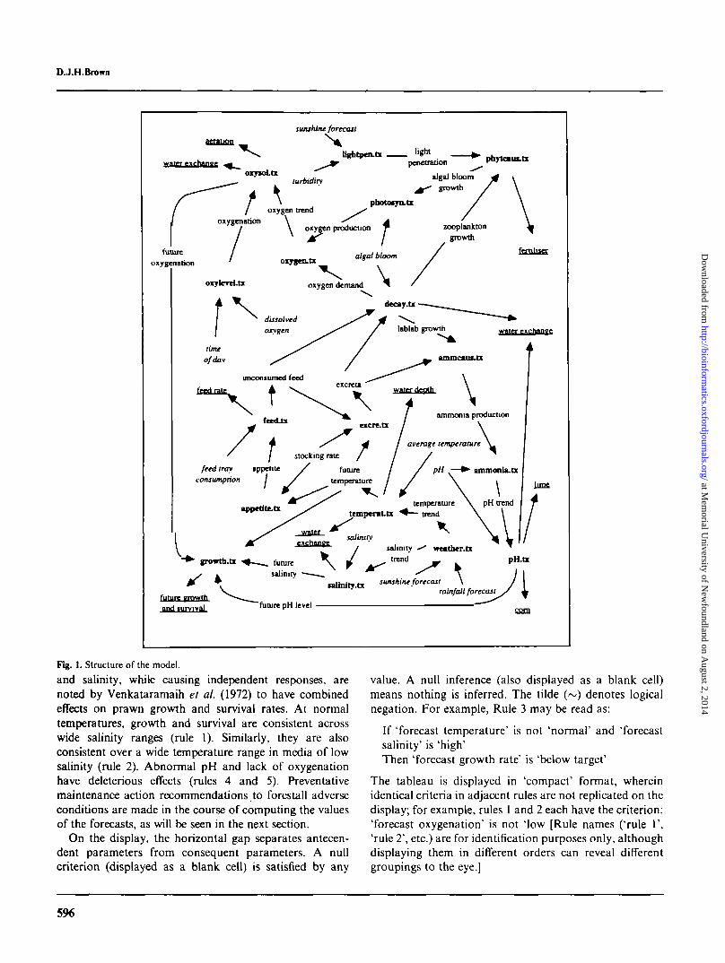
Variation in the production of dissolved oxygen derivesprincipally from variation in photosynthetic activity,which is a function of the density of the phytoplanktonbloom and its growth rate (Romaire el al., 1978), asmodelled by the rules of the tableau photosyn.tx (Figure6). Controlling the bloom is very difficult (Goldman andRyther, 1976; Boyd, 1979), but it is necessary asphytoplankton and paniculate organic matter dynamicsare the principal determinants of conditions in the pond(Piedrahita, 1986).

The 'algal bloom growth rate' is computed by the rulesin the tableau phytcaus.tx (Figure 7). Light is an importantelement needed for phytoplankton (algal bloom) growth;lack of sufficient sunlight due to consecutive rainy orcloudy days can result in reduced growth (rule 1).However, with a low algal biomass, irradiance is unlikelyto limit algal growth even on a dull day (rule 12). In fact,

phote«yej.txrFile Edit Qptions Utility Qheck Inference

Rule]

Rule 4

Rule 1

algal bloomgrowth

low

normal

algal bloom

thin

dense

oxygenproduction

low

high

• • £ ' • * - * •

File Edit SJlilitV Check Interencr

Rulel

Rule 11

Rule 4

RuleS

RuleS

Rule 2

Rule 12

lightpenetration

low

high

low

"high

zooplanktongrowth

high

T.lgh

waterexchange rate

high

low

"high

algal bloom

dense

thin

thin

• I f al bloomgrowth

low

normal

Fig. 7. phytcaus.tx.

the reverse may be true; under hot conditions in brightsunshine, algal growth may be inhibited (photo inhibition)in low turbidity cultures (rule 11). Phytoplankton popula-tions can decrease as a result of an increase in the rate ofzooplankton growth as zooplankton feed on bacteria andminor phytoplankton (Piedrahita, 1986). A large zoo-plankton population can reduce phytoplankton popula-tions because of nutrient limitation on one hand andzooplankton predation (grazing pressure) on the other(rule 4). Fertilizer application has been shown to increasethe chlorophyll levels in fresh water ponds (Boyd, 1973;Rubright et al., 1981).

With proper water exchange management, algae can bemaintained in their growth phase; this is important as fast-growing algal productions are less prone to algal die-offs(Laws and Malecha, 1981; Smith, 1987). Ignoring for themoment the grazing pressure, the pond behaves as acontinuous culture where the water exchange ratecorresponds to the dilution rate. If the dilution rateexceeds the maximum growth rate, the culture will bewashed out (rule 5). At just below the critical dilution ratethe culture will maintain itself with the cells growing at

File Edit Qptions Utility Check Inference

secchi depth

forecastsunshine

lightpenetration

turbidity

Rulel Rule? Rule 3

<n

high

high

low

low

normal

normal

low

Rule 4

>=23

low

high

Fig. 6. photosyn.lx. Fig. 8. lightpen.tx.

598

at Mem


ewfoundland on A



ownloaded from


A qualitative ecological model to support mariculture pond water quality management

ft MUMElle Edit Options Utility

algal bloom

unconsumedfeed

excreta

colour ofwater

turbidity

oxygendemand

lablab growth

zooplanktongrowthwater

exchange

Rulei

Check Inferrncc

Hule2

high

Rule 3

thin

RuleS

high

BBHRule 4

denBe

•high

low

milky white 'milky whHe

high

high

high

33X

• n •• • • —

low

normal

steady

•aM&i

I*

ft.

-


Fig. 9. decay tx.

their maximum growth rate but the biomass will be low(rule 2). As the dilution rate is reduced further, thebiomass will build up but the growth rate will fall asaverage light levels and nutrient availability per cell arereduced (rule 6).

Light penetration into the pond is judged by lightpen.tx(Figure 8) to be inversely proportional to the secchi depth(Davis, 1992). As the model endeavours to predict futureconditions in the pond, the forecast degree of sunshine isused to anticipate future photosynthetic activity based onthe current state of the phytoplankton bloom and itsinferred growth rate.

In the scenario, 'secchi depth' is 23 cm and 'forecastsunshine' is 'high'. Consequently, rule 4 of lightpen.txinfers 'light penetration' is 'low' and 'turbidity' is 'high'.As will be seen later, the Matcher also establishes'zooplankton growth' is 'high', from which rule 4 infers'algal bloom growth rate' is 'low'. Consequently theMatcher infers 'algal bloom growth rate' is 'low'. Becauseof this, and the observation 'algal bloom' is 'thin',photosyn.tx infers 'oxygen production' is 'low'.

Oxygen demand

The tableau decay.tx (Figure 9) infers the oxygen demandin the pond, which is roughly proportional to the lablabgrowth rate (Asian Shrimp News, 1991). (Prawn respira-

Rule 1

Rule?

Rule 3

Rule 1

RuleS

leed trayconsumption

high

normal

low

appetHe

normal

low

i^. II teed rateprawn heal thJ l d J l | s | n l < ! n t

good

poor

increase

ok

reduce

stop

unconsumedfeed

low

ok

high

Fig. 11. Iixd.lv

tion also affects the oxygen demand. This could bereflected by including, for example, stocking densitycriteria in the antecedents of rules in decay.tx.) Highamounts of unconsumed feed and/or excreta contribute tolablab growth (rules 1 and 2). When the water lacks adense phytoplankton bloom and is sufficiently clear toallow sunlight to reach the pond bottom, benthic algaegrow rapidly, stimulating lablab growth (rule 3).

Phytoplankton mortality is usually proportional to thelevel of the phytoplankton bloom, but mass death(evidenced by a milky white colour to the water) causesabnormally high lablab growth (rule 5). Losordo (1980)reports that flushing is the most widely used tactic fortreating sudden mass algal mortality in aquacultureponds, but Busch and Flood (1979) found that flushingdid not prove to be an effective preventative measure.Zooplankton growth is stimulated by an increase inlablab. as the zooplankton feed on its bacterial biomass(rules 1, 2, 3 and 5).

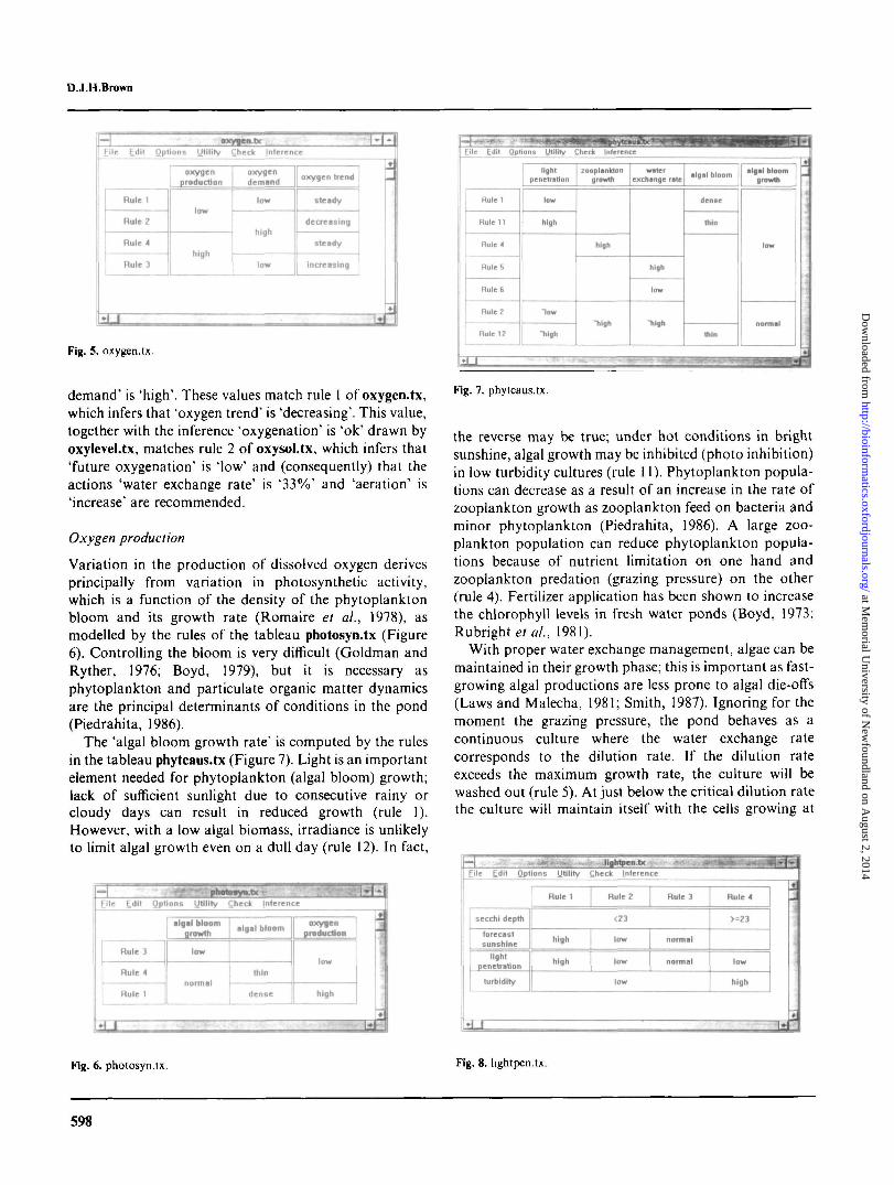
The level of excreta is inferred by extre.tx (Figure 10).High temperatures, feeding rates and stocking densitiestend to increase stress or activity levels in prawns whichlead to high rates of waste excretion (rules 1, 2, 3).

Feed rates are normally determined by reference tostandard estimates of survival. The tableau feed.tx (Figure11) determines whether adjustment to the feeding rate isnecessary and infers the rate of excreta required byexcre.tx. If the consumption rate is higher (lower) thanexpected, it can be assumed that the feed rate is too low(too high). (A common practice in Asian mariculturefarms is to put a proportion of the total feed into feeding

Fjle Ldil Options Utility Check Inference

Rule 1

Rule 2

Rule 3

Rule *

forecasttemperature

high

ttigh

unconsumedfeed

high

Tligh

slockingdensity

l o w

high

-high

excreta

high

normal

Fig. 10. excre.tx.


forecasttemperaturephase of the

moon

Rule 1

'normal

Rule? Rule 4

new, tull

prawn health poor

Rule 3

normnf

quarter.half

appetite

Fig. 12. appeti te . t \ .

599

at Mem


ewfoundland on A



ownloaded from


D.J.H.Brown

llo £dh Options Utility

RulcS

Role 9

Flu I t 4

Rale 6

Rutc7

Rute2

Rate 1

Rule 3

RuJcS

ibecfc Inference • • • £temperature

<28

>-2S* <-32

>32

temperaturetrcod

steady

decreasing

Increasing

steady

decreasing

Increasing

tleady

decreasing

forecasttemperature

low

nonul

low

high

normal

water depth

Increase

3

•LJ L»*

Rg. 13. temperat.tx

trays, whereupon consumption can be checked.) Low feedtray consumption rates may also indicate stress or diseasein the prawns (Davis, 1992). Checks of prawn health,including examination of stomach contents, may benecessary (healthy, well-fed prawns always have fullstomachs). If the prawns appear to be stressed or diseased,feeding and fertilization should be postponed until thesituation is remedied. The value of "appetite' is estimatedby appetite.tx (Figure 12). Appetites are reduced inabnormal temperatures and also during moulting, whichoccurs during new and full moons.

In the scenario, the Matcher establishes "forecasttemperature' is 'normal' (see below), whence it infers'appetite' is 'low' because "phase of the moon' is "new'.This, plus the observations that 'feed tray consumptionrate' is 'low' and 'prawn health' is 'good', match rules 3and 4 of feed.tx, yielding the inferences: 'unconsumedfeed' is 'high' and 'feed rate' is "too high'. To determine thevalue of the parameter 'excreta' of decay.tx. the Matcherexamines the tableau excre.tx (Figure 11). The inference'unconsumed feed' is 'high' drawn by feed.tx is counter-

•a

=llc Edit Option! JJtfirty

RsteS

Rule 3

R.k4

Rale 5

Rale 2

Rule 1

Rute7

R a l e l

forecastratnrafl

heavy

light

none

Hfhtnonc

heavy

£heck Infer

stmsJrfat

normal

"low

bkjb

low

race

watsrBxcfaanM rate

hhjk

normal

low

~M|h

MMhsmperstura

treaJ

steady

Increasing

decreasing

•HEssPntty trend

steady

Increasing

decreatJag

• L l *

pie Edit Option! Utility Check

Rale 6

Rule 7

RuleS

Rote 1

Rule 3

Rule 4

Rttte2

Role 5

RoleB

inanity

>30

>= 20 t <-30

>30

aafinNy trend

decreasing

•ready

Increasing

decreasing

steady

increasing

decreasing

steady

Increasing

forecastfalln.Hu

normal

Ugh

very high

very low

low

norm si

low

Dormal

high

water

33X

33*

33%

•JJ=

Fig. 14. weather tx.

Fig. 15. salinity.tx

balanced by 'stocking density' is 'low' and the inferencedrawn by temperat.tx that 'future temperature' is Mow', sorule 4 of excre.tx matches, which infers 'excreta' is'normal'. This notwithstanding, the values 'unconsumedfeed' is 'high', 'algal bloom' is 'thin' and 'colour of water'is 'brown' match rules 1 and 3 of decay.tx, from which it isinferred that 'oxygen demand' is 'high', "lablab growth' is'high' and 'zooplankton growth' is 'high'.

Forecasting temperature and salinity

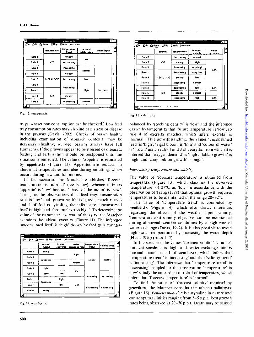
The value of 'forecast temperature' is obtained fromtemperat.tx (Figure 13), which classifies the observed'temperature' of 27°C as 'low' in accordance with theobservation of Tseng (1988) that optimal growth requirestemperatures to be maintained in the range 28-32°C.

The value of 'temperature trend' is computed byweather.tx (Figure 14), which also draws inferencesregarding the effects of the weather upon salinity.Temperature and salinity objectives can be maintainedduring abnormal weather conditions by a high rate ofwater exchange (Davis, 1992). It is also possible to avoidhigh water temperatures by increasing the water depth(Huet, 1970) (rules 1-3).

In the scenario, the values 'forecast rainfall' is 'none','forecast sunshine' is 'high' and 'water exchange rate' is'normal' match rule 1 of weather.tx, which infers that"temperature trend' is 'increasing' and that 'salinity trend'is 'increasing'. The inference that 'temperature trend' is'increasing' coupled to the observation 'temperature' is'low' satisfy the antecedent of rule 4 of temperat.tx, whichinfers that 'forecast temperature' is 'normal'.

To find the value of 'forecast salinity' required bygrowth.tx, the Matcher consults the tableau salinity.tx(Figure 15). Penaeus monodon is euryhaline in nature andcan adapt to salinities ranging from 3-5 p.p.t., best growthrates being observed at 20-30 p.p.t. Death may be caused

600

at Mem


ewfoundland on A



ownloaded from


A qualitative ecological model to support marimlture pond water quality management

Elle Edit Options UtBHy Caedc Inference

Rulo 1

Rale 4

R d e 3

RuteE

Rulo2

Rule 5

Rule 7

PH

>-S.5

<7

>-7 1 <9.5

pH trend

decreasing

Increasing

decreasing

Increasing

decreasing

steady

forecast pH

very high

aormal

very low

Irlgh,

law

normal

addMve

com

lime

com

lime

water

SOX

set

33X

JO.

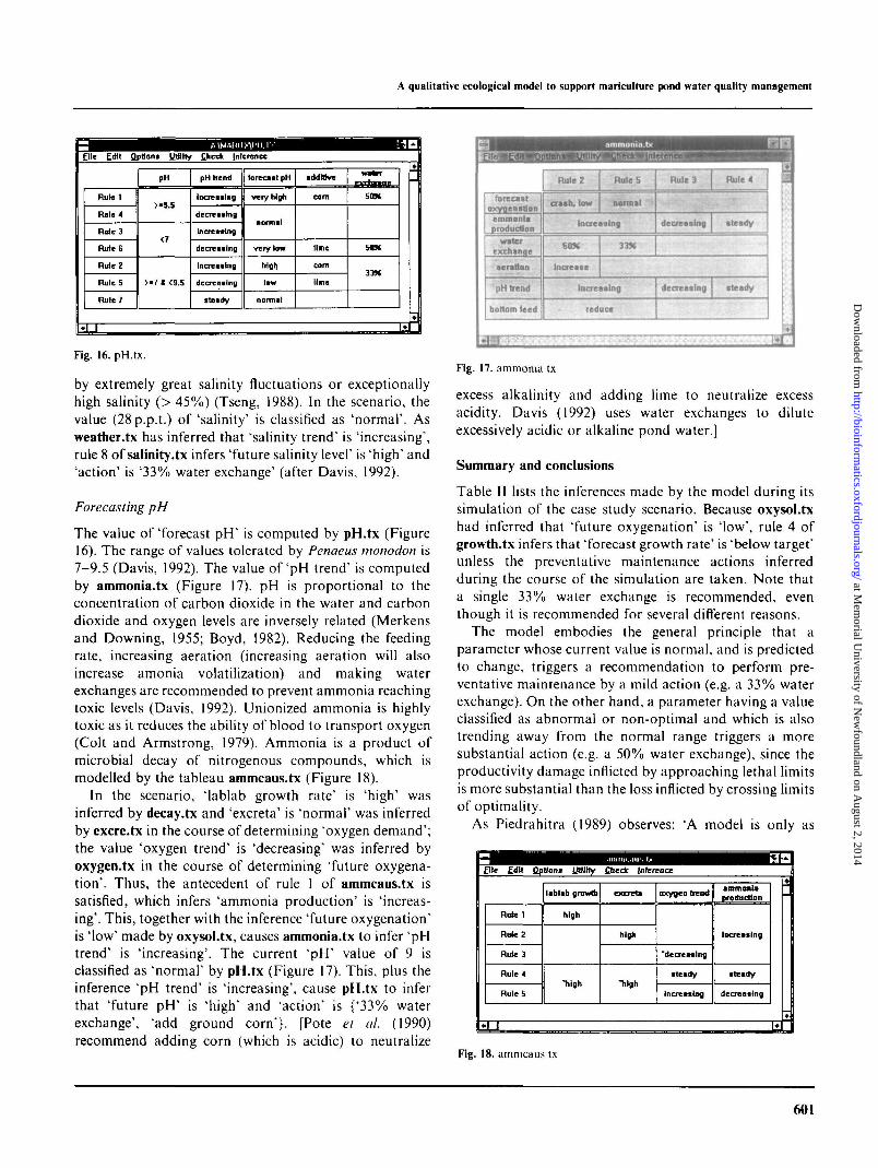
Fig. 16. pH.tx.

by extremely great salinity fluctuations or exceptionallyhigh salinity (> 45%) (Tseng, 1988). In the scenario, thevalue (28p.p.t.) of 'salinity' is classified as 'normal'. Asweather.tx has inferred that 'salinity trend' is 'increasing',rule 8 of salinity, tx infers 'future salinity level' is 'high' and'action' is '33% water exchange' (after Davis, 1992).

Forecasting pH

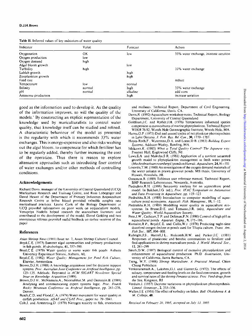
The value of 'forecast pH' is computed by pH.tx (Figure16). The range of values tolerated by Penaeus monodon is7-9.5 (Davis, 1992). The value of'pH trend' is computedby ammonia.tx (Figure 17). pH is proportional to theconcentration of carbon dioxide in the water and carbondioxide and oxygen levels are inversely related (Merkensand Downing, 1955; Boyd, 1982). Reducing the feedingrate, increasing aeration (increasing aeration will alsoincrease amonia volatilization) and making waterexchanges are recommended to prevent ammonia reachingtoxic levels (Davis, 1992). Unionized ammonia is highlytoxic as it reduces the ability of blood to transport oxygen(Colt and Armstrong, 1979). Ammonia is a product ofmicrobial decay of nitrogenous compounds, which ismodelled by the tableau ammcaus.tx (Figure 18).

In the scenario, Mablab growth rate' is 'high' wasinferred by decay.tx and 'excreta' is 'normal' was inferredby excre.tx in the course of determining 'oxygen demand';the value 'oxygen trend' is 'decreasing' was inferred byoxygen.tx in the course of determining 'future oxygena-tion'. Thus, the antecedent of rule 1 of ammcaus.tx issatisfied, which infers 'ammonia production' is 'increas-ing'. This, together with the inference 'future oxygenation'is 'low' made by oxysol.tx, causes ammonia.tx to infer 'pHtrend' is 'increasing'. The current 'pH' value of 9 isclassified as 'normal' by pH.tx (Figure 17). This, plus theinference 'pH trend' is 'increasing', cause pH.tx to inferthat 'future pH' is 'high' and 'action' is {'33% waterexchange', 'add ground corn'}. [Pote ei al. (1990)recommend adding corn (which is acidic) to neutralize

force* t toxygenaHoB

ammoniaproduction

waterexchange

aeration

pH trend

bottom feed

RuleZ

ara*fe,low

Rale 5

normal

Increasing

SOX

increase

33%

Rule 3 Rule 4

decreasing steady

Increasing

• reduce

decreasing steady

Fig. 17. ammonia tx

excess alkalinity and adding lime to neutralize excessacidity. Davis (1992) uses water exchanges to diluteexcessively acidic or alkaline pond water.]

Summary and conclusions

Table II lists the inferences made by the model during itssimulation of the case study scenario. Because oxysol.txhad inferred that 'future oxygenation' is Mow", rule 4 ofgrowth.tx infers that 'forecast growth rate' is "below target"unless the preventative maintenance actions inferredduring the course of the simulation are taken. Note thata single 33% water exchange is recommended, eventhough it is recommended for several different reasons.

The model embodies the general principle that aparameter whose current value is normal, and is predictedto change, triggers a recommendation to perform pre-ventative maintenance by a mild action (e.g. a 33% waterexchange). On the other hand, a parameter having a valueclassified as abnormal or non-optimal and which is alsotrending away from the normal range triggers a moresubstantial action (e.g. a 50% water exchange), since theproductivity damage inflicted by approaching lethal limitsis more substantial than the loss inflicted by crossing limitsof optimality.

As Piedrahitra (1989) observes: 'A model is only as

pie EdU Qotlons jpJIhy Check Inference

Hotel

Rote?

Ride 3

Rule 4

Rule 5

lablah growth

high

"high

OCCfCtA

hlgk

"high

oxygen trend

"decreasing

steady

Incrcastog

•ratnomlaproduction

Increasing

steady

decreasing

Fig. 18. ammcaus tx

601

at Mem


ewfoundland on A



ownloaded from


D.J.H. Brown

Table II. Inferred values of key indicators of water quality

Indicator Value Forecast Action

OxygenationOxygen productionOxygen demandAlgal bloom growthTurbidityLablab growthZooplankton growthFeed rateTemperatureSalinityPHAmmonia production

OKlowhigh

high

lownormalnormal

low

low

highhigh

normalhighalkalinehigh

33% water exchange, increase aeration

33% water exchange

reduce

33% water exchangeadd cornincrease aeration

good as the information used to develop it. As the qualityof the information improves, so will the quality of themodels.' By constructing an explicit representation of theknowledge used by mariculturalists to control waterquality, that knowledge itself can be studied and refined.A characteristic behaviour of the model as presentedis the regularity with which it recommends 33% waterexchanges. This is energy-expensive and also risks washingout the algal bloom, to compensate for which fertilizer hasto be regularly added, thereby further increasing the costof the operation. Thus there is reason to explorealternative approaches such as introducing finer controlof water exchanges and/or other methods of controllingconditions.

Acknowledgements

Richard Davis, manager of the University of Central Queensland (UCQ)Mariculture Research and Training Centre, and Ross Lobegeiger andDavid Hewitt of the Department of Primary Industries AcquacultureResearch Centre at bribie Island provided valuable insights intomaricultural practices. Laune Cook of the Biology Department atUCQ provided information on prior work on acquaculture models.Venupriya Nadella helped research the manculture literature andcontributed to the development of the model. David Golding and twoanonymous referees provided useful feedback on earlier versions of thispaper

References

Asian Shrimp News (1991) Issue no 7, Asian Shrimp Culture Council.Boyd.C.E. (1973) Summer algal communities and primary productivity

in fish ponds. Hydrobiologia, 41, 357-390.Boyd.C E. (1979) Water quality in warm water fish ponds Auburn

University Experiment Station. Auburn, ALBoyd.C.E. (1982) Water Quality Management for Pond Fish Culture.

Elsevier, AmsterdamBrown,D.J.H. (1988) A knowledge acquisition tool for decision support

systems. Proc. Australian Joint Conference on Artificial Intelligence, pp125-135, Adelaide. Reprinted in ACM S1GART Newsletter SpecialIssue on Knowledge Acquisition (1989).

Brown,DJ H . McNamara.A.. Noormfshar.M. and Orenstein.B. (1989)Analysing and communicating expert systems logic. Proc. FourthRocky Mountain Conference on Artificial Intelligence, pp. 261-276.Denver.

Busch.C.D. and Flood,C.A. (1979) Water movement for water quality incatfish production. ASAE and CSAE Proc, paper no. 79-5041.

Colt.J. and Armstrong.D (1979) Nitrogen toxicity to fish, crustaceans

and molluscs. Technical Report. Department of Civil Engineering.University of California, Davis. CA.

Davis,R (1992) Aquaculture workshop notes. Technical Report, BiologyDepartment, University of Central Queensland

GoldmanJ.C. and Ryther,J.H. (1976) Temperature influenced speciescompetition in mass cultures of marine phytoplankton. Technical ReportWHOI 76-92, Woods Hole Oceanographic Institute, Woods Hole, MA.

Harris,G.P. (1973) Diel and annual cycles of net plankton photosynthesisin Lake Ontario. J. Fish. Res. Bd. Can , 30, 1779-1787.

Hayes-Roth,F , Waterman.D A. and Lenat.D B. (1983) Building ExpertSystems. Addison-Wesley, Reading, MA.

Ishikawa.K. (1985) What is Total Quality Control' The Japanese way.Prentice Hall, Englewood Cliffs, NJ.

Laws.E.A and Malecha,S R. (1981) Application of a nutrient saturatedgrowth model to phytoplankton management in fresh water prawn(Machrobrachium rosenbergii) ponds in Hawaii. Aquaculture, 24,91 -101

Losordo,T.M. (1980) An investigation of the oxygen demand materials ofthe water column in prawn growout ponds. MS thesis, University ofHawaii, Honolulu, HI.

Orenstein.B. (1989) Tableaux user reference manual. Technical Report,BHP Research Laboratories, Newcastle, Australia.

Piedrahita.R.H. (1986) Sensitivity analysis for an aquaculture pondmodel. In Balchen.J.G (ed.), Proc IFAC Symposium on Automationand Data Processing in Aquaculture, pp. 119-123

Piedrahita.R.H. (1988) Introduction to computer modelling of aqua-culture pond ecosystems. Aquacull. Fish. Managmnt., 19, 1-12.

Piedrahita,R.H. (1989) Modelling water quality in aquaculture eco-systems. In Brune,D.E. and Tomasso.J.R. (eds), Aquaculture andWater Quality. World Aquaculture Society.

Pote.J.W , Cathcart,T P. and Deliman.P.N. (1990) Control of high pH inaquacultural ponds Aquacull. Engng., 9, 175-186.

Romaire,RP., Boyd.C.E. and Collis,W.J (1978) Predicting night-timedissolved oxygen decline in ponds used for Tilapia culture. Trans Am.Fish Soc, 107, 804-808.

Rubnght,J.S, HarrellJ L.. Holcomb.H.W. and Parker.J.C (1981)Responses of planktonic and benthic communities to fertilizer andfeed applications in shrimp manculture ponds J. World Maricul Soc,12,281-299

Smith.D.W. (1987) Biological control of excessive phytoplankton andenhancement of aquacultural production P h D dissertation. Uni-versity of California, Santa Barbara, CA.

Tseng, W.Y. (1988) Shrimp Mariculture. A Practical Manual. ChienCheng Publishers

Venkataramaih,A., Lakshrru,G.J. and Gunter,G. (1972). The effects ofsalinity, temperature and feeding levels on the food conversion, growthand survival rates of the shrimp Penaeus azlecus. Proc Feed-drugs fromthe Sea. Kingston, Rl

Verduin.J. (1957) Daytime variations in phytoplankton photosynthesis.Limnol Oceanogr., 2, 333-336.

Wallen.I.E (1951) The effect of turbidity on fishes. Bull OkalahomaA.&M. College, 48.

Received on February 20. 1995, accepted on July 13. 1995

602

at Mem


ewfoundland on A



ownloaded from


a qualitative ecological model to support mariculture pond water quality management

Documents