a pseudospectral method for two-point boundary value problems

JOURNAL OF COMPUTATIONAL PHYSICS 88, 1699182 (1990)

A Pseudospectral Method for Two-Point Boundary Value Problems

S. J. JACOBS

Department of Atmospheric, Oceanic, and Space Sciences, Department of Mechanical Engineering and Applied Mechanics,

University of Michigan, Ann Arbor, Michigan 48109

Received June 3, 1988; revised July 18, 1989

Pseudospectral collocation is employed for the numerical solution of nonlinear two-point boundary value problems with separated end conditions. Second-order finite difference schemes are used as preconditioners for the spectral calculation, and a solution of the discretized equations is obtained using versions of the defect correction principle. The method and a variant based on an adaptive grid technique are tested on a variety of sample problems and are shown to provide high accuracy with low storage requirements. 6 1990 Academic

Press, Inc.

1. INTRODUCTION

The purpose of the present paper is to present a pseudospectral collocation method for solving the boundary value problem

u’(x) - f[x, u(x)] = 0 (a < x < b), (Ia)

g1 (u(a)) = 0, gAu(b)) = 0,

in which u and f have dimension D, and g, and g, have dimension D, and D,, respectively, with D, + D2 = D. Problems of this type type arise in the study of the stability of atmospheric and oceanic flows, in other applications of fluid mechanics, and in the solution of parabolic initial value problems in one spatial variable w implicit time differencing is employed.

The simplest finite difference methods for solving (1) are based on the implicit midpoint and trapezoidal rules, for which the discretization error is ~ornpar~tiv~l~ large but can be reduced through the use of Richardson extrapolation or deferred corrections [l-3]. In these approaches, solving the discretized equations by Newton iteration is inexpensive because of the narrow bandwidth of the Jacobian matrix. By contrast, programs based on pseudospectral methods [4-S] solve differential equations by collocation using an interpolation polynomial for which the nodes are the extrema or the zeros of an orthogonal polynomial. Pseudospectral collocation is far more accurate than any low-order finite difference method using

169 OOZl-9991190 $3.00

Copyrigh! 0 1990 by Academic Pms, Inc. All rights of reproduction in any form reserved.

170 S. J. JACOBS

the same grid if a sufficient number of grid points is employed, but the Newton iteration part of the computation is expensive because the pseudospectral Jacobian matrix is dense.

Because of this, most applications of pseudospectral collocation employ an iteration procedure in which a preconditioning method is used to approximate the Jacobian matrix by a Jacobian obtained through use of a finite difference discretization. Consequently, the major issues involved in the development of a pseudospectral method for the numerical solution of (1) are the choices of an iteration procedure for solving the discretized equations and of a preconditioning finite difference scheme.

Taking these points in order, it can be seen that treating (1) using pseudospectral collocation with M grid points yields a set of MD equations F(u) = 0, with solution U=U*, where u temporarily stands for the solution evaluated at the grid points, while use of a finite difference method on the same grid requires solving a system G(u) = 0, with solution u”, for which the Jacobian matrix has a narrow bandwidth and is easy to invert. If u” is an isolated solution of G(u) =0 and if IG(u)-F(u)1 is sufficiently small for u in some closed neighborhood of u”, the existence of a unique solution u* of the pseudospectral equations can be proved using a generalization of Rouche’s theorem [S].

To obtain a constructive method for calculating u*, we express the equation F(u)=0 in either of the forms

u=u+u’-G-‘[F(u)], (24

u=G-‘[G(u)-F(u)] G’b)

and employ fixed point iteration to find the solution. The fixed point iteration scheme for (2a) is the Zadunaisky iteration [6]

G(u’) = 0,

U n+l=un+uo-G-l[F(~“)], n = 0, 1, . ..) (3)

also known as version A of the defect correction principle [7], and.the corresponding scheme for (2b) is

G(uO) = 0, (4)

U n+l=G-l[G(u”)-F(u”)], n = 0, 1, . ..)

which is commonly described as version B of the defect correction principle [7]. Here the solution G-‘(c) of the equation G(u) = c is obtained by Newton iteration, and convergence of (3) and (4) can be proved using a version of the contraction mapping theorem [9]. As in the proof of the existence of the solution u*, the crucial point is that the preconditioning method must be chosen such that G is a close approximation to F.

PSEUDOSPECTRAL METHOD 111

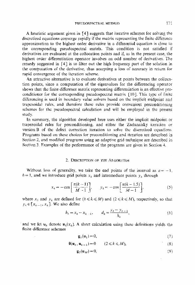
A heuristic argument given in [4] suggests that iterative schemes for solving the discretized equations converge rapidly if the matrix representing the finite difference approximation to the highest order derivative in a differential equation is close to the corresponding pseudospectral matrix. This condition is not satisfied if derivatives are evaluated at the collocation points and if, as in the present case, the highest order differentiation operator involves an odd number of derivatives. The remedy suggested in [4] is to filter out the high frequency part of the solution in the computation of the derivative, thus accepting a loss of accuracy in return for rapid convergence of the iteration scheme.

An attractive alternative is to evaluate derivatives at points between the cohoca- tion points, since a computation of the eigenvalues for the differencing operator shows that the finite difference matrix representing differentiation is an effective pre- conditioner for the corresponding pseudospectral matrix [IO]. This type of finite differencing is used in boundary value solvers based on the implicit midpoint an trapezoidal rules, and therefore these rules provide convenient precondit~~~i~g schemes for the pseudospectral calculation and will be employed in the present study.

In summary, the algorithm developed here uses either the implicit midpoint or trapezoidal rules for preconditioning, and either the Zadunaisky iteration or version B of the defect correction iteration to solve the discretized equations. Programs based on these choices for preconditioning and iteration are described in Section 2, and modified programs using an adaptive grid technique are described in Section 3. Examples of the performance of the programs are given in Section 4.

2. DESCRIPTION OF THE ALGQRITHM

Without loss of generality, we take the end points of the interval as a = - 1, b = 1, and we introduce grid points xk and intermediate points y, through

xk= -cos w ) [ 1 yk z -CQS i @--1;5) where xk and yk are defined for (1 d k d M) and (2 <k G M), respectively, so that yk E [xk _ 1, xk]. We also define

hk=xk-xk--, dk= yk-hyk-1, k

and we let uk denote uk(xk). A short calculation using these definitions yields the finite difference schemes

g,(ul)=o~ VI

e(“k, uk-l)=o (2<k<.M), w

&(U,) = 0, (91

172 S. J. JACOBS

where

0= uk-“k-l

h -f[yks dk”k+ l1 -dk) uk--ll

provides a generalized version of the implicit midpoint rule, and

a generalized version of the trapezoidal rule. The standard versions of these rules are obtained by defining y, as the average of xk _ 1 and xk.

In the pseudospectral method of solving the problem, u and u’ are approximated by

M-l M-1

U(X)= c &T/c(X), u’(x) = c Bk~k(X), k=O k=O

(12)

where T,+(x) are the Chebyshev polynomials defined by

Tk(x) = cos[k cos-l(x)] (13)

and where B, is expressed in terms of A, by the recursion

B -0 M-l- 2 B,,,_2=2(M-1)A,,,--l, (14)

c k+lBk=Bk+2+2(k+l)Ak+l (M-33k30),

in which c1 = cM = 2, ck = 1 for 1 <k < M. The Chebyshev coefficients A, are given in terms of the values of u at the grid points by

2 M-1 UMdj Ak=(M-l)ck j;. zcos (15)

and, for evaluation at the points xk and yk, the sums in (12) as well as the sum (15) can be evaluated through use of fast Hartley transform techniques as described in [ll, 121.

Using the definition of yk given above, the pseudospectral method of treating the boundary value problem consists of solving (7), (9), and

U’(Yk)-f[Yk, u(Yk)l =O (2<k<M). (16)

Hence (7), (8), and (9) define the function G(u) discussed in the previous section, and (7), (16), and (9) the function F(u). The solution of the problem thus reduces to carrying out the outer iteration procedures discussed above, using the linear algebra techniques given in Cl]. In carrying out this calculation the Jacobian of G(u) can be computed either analytically or by numerical differentiation.


The calculation runs as follows. At the start of the program, the user selects an initial value of M, tolerances TOLOUT, TOLNEWT, and TOLCHEB, a maximum number of outer iterations, and a maximum number of Newton iterations. the program increases the number of grid points by replacing M by (2M- grid is too coarse to provide the accuracy specified by the choice of TOL value MAXM for the maximum alowed number of grid points must also be provided. The initial M is chosen such that (M - 1) is an integral power of 2, and so the method used to refine the grid allows the use of a base two fast Hartley transform.

After an initial estimate u” is determined, the program carries out the iterations, with the Newton iteration ended if the relative magnitude of a Newton correction is less than TOLNEWT, and the outer iterations if

IU ??+ l- un/ < jlq . TOLOUT (17)

is satisfied for three successive values of ~1. Upon successful completion of the outer iterations, the program computes the quantities Lk = /Ak/$ LMAX, the maximum of L, over k, and a quantity NORMCHEB defined as the maximum of the ratios of the values of Lk for the three highest order Chebyshev coefficients to L NORMCHEB is less than TOLCHEB, the program ends. If not, a finer grid is selected by replacing M by (2M- l), with the previously calculated values and u(yJ used to provide an initial estimate for the solution on the new gri order to avoid futile calculations on too coarse a grid, a finer grid is also selected if the value of NORMCHEB at the end of the first outer iteration on any grid is larger than IE- 3.

If a finer grid is selected, the calculation continues until the criterion involving TOLCHEB is satisfied or until M= MAXM, the maximum number of grid points allowed for the calculation. For the test problems discussed below, the rna~~m~rn relative error in the solution is within an order of magnitude or so of the value selected for TOLCHEB if MAXM is sufficiently large. In addition, defining the residual norm at each grid point as a norm of the left side of (16), sample calculations show that this norm is also close to TOLCHEB.

The test problems were treated using the programs MZAD and MDEF, which are based on the implicit midpoint rule and either the Zadunaisky iteration or version B of the defect correction principle. Most of the problems were also solved using an adaptive grid version of these programs described in the next section.

3. AN ADAPTIVE GRID VERSION OF THE ALGORITHM

To describe the adaptive grid scheme used in the present study, it is necessary to review adaptive grid methods currently employed in finite difference calculations. These involve two elements, the choice of a criterion for deciding which regions af the domain require additional grid points, and the method by which the re~~eme~t of the grid is implemented.

174 S. J. JACOBS

The most widely used procedures for deciding where the grid should be refined are based on either the magnitude of the local truncation error, as in Lentini and Pereyra’s program PASVAR [2-31, or on the magnitude of the function

W(x) = 1 + Cl Ill’/ + c2 Ju”(, (18)

in which c1 and c2 are non-negative constants. If a criterion for grid modification is known, the grid can be refined either by adding grid points in regions where the solution varies rapidly or by solving the problem using a computational coordinate X= H(x), where the mapping is chosen so that the solution is a smoothly varying function of X. The first method is used in PASVAR, with grid points added so as to distribute the local truncation error equally over X, and the second in a number of papers reviewed in [13].

Because the choice of the grid point locations is not at the user’s disposal in a pseudospectral calculation, adaptive grid refinement for such methods must be based on a mapping technique. Accordingly, in the present study we introduce a positive weight function W(X) defined for x E [a, b] and a mapping X= H(x) through

X=u+~~xw(x’)dx’, (19) a

where

(20)

so that (19) maps the interval [a, b] into itself. Then, defining x = h(X) as the inverse mapping and U(X) as UC/Z(X)], (1) becomes

U’(X) - wlhyx)l fCw0 w31 = 0 (a<X<b), (214

g1 W(a)) = 03 &W(b)) = 0. @lb)

If 5 lies in [x, x + Sx] and if the corresponding region in the computational space is [X, X+ SX], the mean value theorem for Riemann integrals shows that 6X= [w(s)/01 6x. It can be seen that if w is chosen to be large in regions where u varies rapidly and if 6X is fixed, then 6x is small and the mapping effectively adds grid points where they are needed.

As before, we can take the end points of the interval as a = - 1, b = 1, without loss of generality. If w(x) is known the integrals in (19) and (20) can be determined by expanding w in a Chebyshev series of the form (12) and by integrating this series term by term, and the inverse mapping x = h(X) by solving (19) numerically. The solution of (21) can then be carried out as before, and hence the major remaining problem in developing a pseudospectral adaptive grid scheme is that of finding a suitable weight function.


In one such scheme [ 141, the grid is refined by taking w as a function F(x, yY c), where F peaks strongly at a single point y and where the magnitude of the constant c determines the height and width of the peak. In [14], y and c are determined by computing the solution to a certain degree of accuracy on the original grid, evafuat- ing a Sobolev type semi-norm as a function of these quantities, and choosing to minimize the semi-norm. Despite the success of this method as implement [14], it is clear that defining w as a function which peaks at a single point is too specialized to be of general use, and therefore we prefer taking the weight function as the function W(x) defined above in Eq. (18).

In our first try at devising an adaptive grid scheme using W as a weight function, the constants c1 and c2 were given various values and the accuracy of solutions obtained using the adaptive and original grids was compared for a fixed number of grid points. Although W peaks where it should, in regions of rapid variation of the solution, use of the adaptive method with user supplied values of c1 and c2 decreases the accuracy of the solutions in many cases. It appears that the method fails because W is both sharply peaked and noisy in difficult problems, an therefore we found it necessary to apply a low pass filler to W in order to obtain solutions of (21) with spectral accuracy. This is accomplished by taking ci = c2 = 1 in (18 ), by expanding the resulting expression for W in the form

M-l

W= c a,T,(x),

k=O

and by taking w as

M-1

w(x) = 1 ak exp( -;lk) Tk(x), k=O

(23)

where Jti is a damping constant. This constant must be chosen to smooth the weight function without losing the structure entirely.

Current versions of the adaptive grid scheme proposed here allow two methods for choosing the damping constant, both of which require an initial finite di~ere~~~ iteration and outer iteration on the original Chebyshev grid to calculate W. In the first option the damping constant is determined numerically so that

Max {a,exp(-X)) <lE-I5 k

In the other, the region LE [0, co] is mapped into M E [amin, I], where, recalling that xk (1 <k d M) are the Chebyshev grid points and that X= H(x) is the computational coordinate, the mapping CI = a(]+) is defined in terms of a rni~~rn~rn step size ratio by

176 S.J. JACOBS

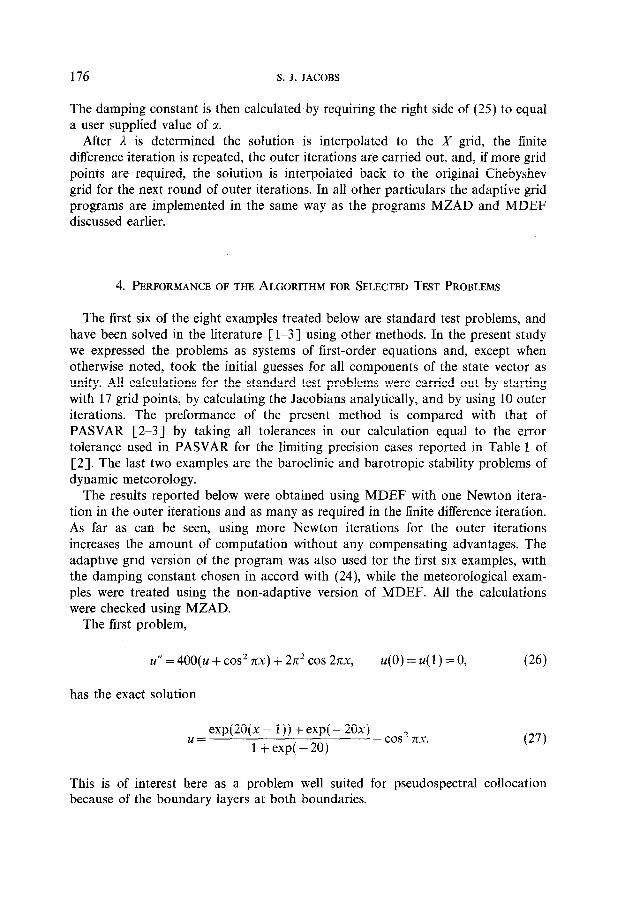
The damping constant is then calculated by requiring the right side of (25) to equal a user supplied value of CI.

After 2 is determined the solution is interpolated to the X grid, the finite difference iteration is repeated, the outer iterations are carried out, and, if more grid points are required, the solution is interpolated back to the original Chebyshev grid for the next round of outer iterations. In all other particulars the adaptive grid programs are implemented in the same way as the programs MZAD and MDEF discussed earlier.

4. PERFORMANCE OF THE ALGORITHM FOR SELECTED TEST PROBLEMS

The first six of the eight examples treated below are standard test problems, and have been solved in the literature [l-3] using other methods. In the present study we expressed the problems as systems of first-order equations and, except when otherwise noted, took the initial guesses for all components of the state vector as unity. All calculations for the standard test problems were carried out by starting with 17 grid points, by calculating the Jacobians analytically, and by using 10 outer iterations. The preformance of the present method is compared with that of PASVAR [2-31 by taking all tolerances in our calculation equal to the error tolerance used in PASVAR for the limiting precision cases reported in Table 1 of [2]. The last two examples are the baroclinic and barotropic stability problems of dynamic meteorology.

The results reported below were obtained using MDEF with one Newton iteration in the outer iterations and as many as required in the finite difference iteration. As far as can be seen, using more Newton iterations for the outer iterations increases the amount of computation without any compensating advantages. The adaptive grid version of the program was also used for the first six examples, with the damping constant chosen in accord with (24), while the meteorological examples were treated using the non-adaptive version of MDEF. All the calculations were checked using MZAD.

The first problem,

u” = 4OO(U + cos2 nx) + 27c2 cos 27rx, u(O)=u(l)=O, (26)

has the exact solution

u = exp(2O(x - 1)) + exp( -20.4 _ cos2 71x 1 + exp( -20) (27)

This is of interest here as a problem well suited for pseudospectral collocation because of the boundary layers at both boundaries.

PSEUDOSPECTRAL METHOD $77

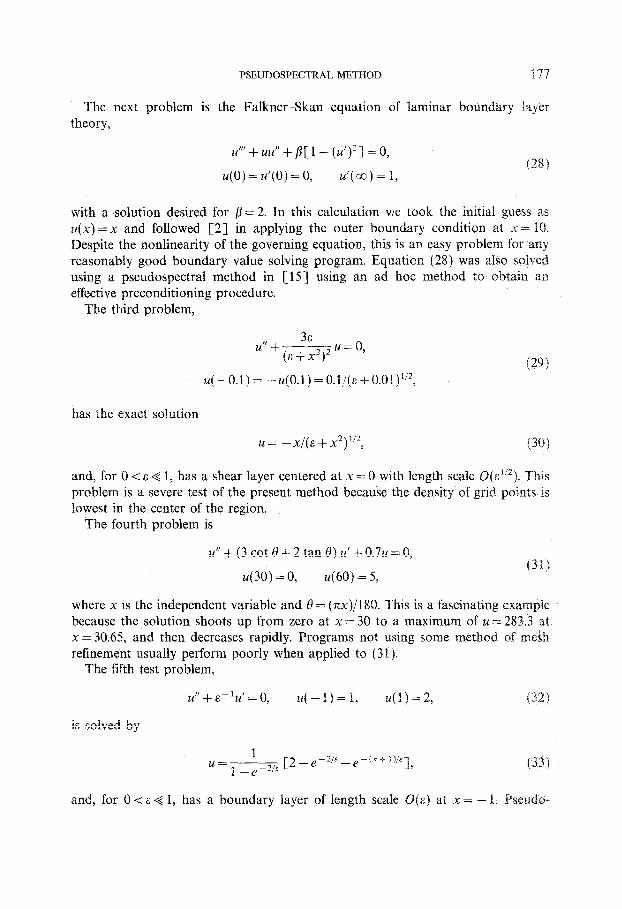
The next problem is the Falkner-Skan equation of laminar boundary layer theory,

u”’ + UU” + p[l - (U’)2] = 0,

u(0) = u’(0) = 0, u’(a) = I, (28)

with a solution desired for p = 2. In this calculation we took the initial guess as u(x) =x and followed [2] in applying the outer boundary condition at x = IO. Despite the nonlinearity of the governing equation, this is an easy problem for any reasonably good boundary value solving program. Equation (28) was also solve using a pseudospectral method in [15] using an ad hoc method to obtain an effective preconditioning procedure.

The third problem,

3E d + (E + x2)2 24 = 0,

1291 U(-o.i)= -u(0.1)=0.1/(E+0.0~)“2,

has the exact solution

u = -X/(& + x2y2: (30)

and, for 0 < F 4 1, has a shear layer centered at x = 0 with length scale O(E”‘). This problem is a severe test of the present method because the density of grid points is lowest in the center of the region.

The fourth problem is

U” + (3 cot 0 + 2 tan 0) 24’ + 0.724 = 0,

2.4 30) = 0, 460) = 5, (311

where x is the independent variable and 8 = (nx)/180. This is a fascinating example because the solution shoots up from zero at x = 30 to a maximum of u = 283.3 at x = 30.65, and then decreases rapidly. Programs not using some method of mesh refinement usually perform poorly when applied to (31).

The fifth test problem,

is solved by

Zl" + E -'u'=Q, U(-l)=E, u(1)=2, (321

1 Id= 1 -e~2,E [2-e-2/“--e(““i)/&],

and, for 0 <E < 1, has a boundary layer of length scale O(E) at x = - 1.

178 S. .I. JACOBS

spectral schems can be expected to be inefficient in solving this problem because the high resolution provided by such schemes at the right end point is wasted.

The final standard test problem is defined by

24’ = u3 - sin(x)[ 1+ sin2(x)], u(0) = U(7c) = 0, (34)

with solution u = sin(x). This was worked here and in [2] as an example of an easy problem.

In the summary of results shown in Table I the errors are the actual maximum errors in the solution for Problems 1, 3, 5, and 6, while, for Problems 2 and 4, the listed errors are an error tolerance TOL for the PASVAR results and the tolerance TOLCHEB for the results obtained using the present method. The number of equivalent function evaluations in the table is the sum (F+ wJ), where F is the number of function evaluations, J is the number of Jacobian evaluations, and w is a weighting constant. Values of the weighting constant for each problem are given in [2] along with a rationale for using the number of equivalent function evaluations as a means of evaluating the efficiency of the computation.

Although it may be paradoxical to describe calculations with errors less than lE- 17 as disappointing, there is no doubt that the present method performs poorly as compared to PASVAR when applied to the easy problems, 2 and 6. A dif- ficulty in computing efficiently using a pseudospectral scheme is that the method sometimes works too hard in the process of attaining more accuracy than needed. This does not always occur; for example, MDEF solves the standard test problem

u” = e”, u(0) = u( 1) = 0,

with an error of lE- 17 using only 900 equivalent function evaluations and 17 grid points. However, excessive computing can occur in a pseudospectral scheme and is one of its weaknesses. Its strength, as shown by the fact that the adaptive version of MDEF required only 65 grid points even for the most difficult problems treated here, is its combination of high accuracy and low storage requirements.

TABLE I

Comparison of Present Method with PASVAR

Problems 1 2 3 4 5 6

El 1.6E- 12 l.OE- 14 7.8E-11 1.6E-11 8.2E-11 l.OE- 14 E2 5.3E- 14 8.9E-20 1.6E- 15 4.4E- 19 9.5E-15 9.3E- 18 E3 5.3E- 13 1.9E-18 1.9E - 13 l.OE-15 9.0- 14 2.OE- 16 Fl 2096 3438 3559 9827 3212 747 F2 2203 6480 10,212 10,712 10,060 2400 F3 2635 8365 5776 4743 4439 3483

Motes. Absolute error in calculation: El, PASVAR; E2, MDEF; E3, Adaptive MDEF. Equivalent function evaluations: Fl, PASVAR; F2, MDEF; F3, Adaptive MDEF.


Turning next to the boundary layer problems, 1 and 5, it can be seen that k non-adaptive version of MDEF does well on problem 1 and poorly on problem for reasons indicated above, and, correspondingly, the present adaptive gr fails to improve the efficiency of the calculation for problem 1, but does so for problem 5. Finally, as regards the internal shear layer problems 3 and 4, these resemble problem 5 in the sense that use of an adaptive grid scheme greatly improves the efficiency of the calculation for all three problems. In these problems use of the adaptive grid version of MDEF decreases the number of equivalent function evaluations and the number of collocation points required for attaining t desired accuracy by a factor of two.

Ranking the performance of the programs on this set of problems is difficult. It is clear that the adaptive version of MDEF is more efficient than PASVA working problem 4 and that PASVAR is better in dealing with problems 2 and 6. Deciding which program is superior in dealing with the other problems depends on the weight placed by the user on the amount of computation as compared to the accuracy of the results.

In addition to these calculations, problems 3 and 5 were worked using an a tive grid scheme based on (25), in which the user supplies a value a of the minimum step size ratio on the right side of that equation. In these cases the choice m = 0.625 provides considerable improvement of the results over those given in Table I in terms of efficiency and accuracy, thus suggesting that it might be possible to developed a method for choosing an optimal damping constant.

The last two examples are taken from the quasigeostrophic theory of atmospheric flow. Letting (x, y, z) denote distance to the east, the north, and in the vertical, the inviscid version of the theory admits as a solution an arbitrary flow U( y, z) in the x-direction. The stability of this flow can be determined using a linear st&il&y analysis with the pressure pertubation expressed as the real part of

$(Y, z) exp[IW- ct)l,

where CI > 0 and where t denotes time. Here the complex phase velocity c is an eigenvalue, and the flow is unstable if ci, the imaginary part of c, is positive. In the baroclinic stability problem it is assumed that U and + depend only on z, while in the barotropic problem U and $ depend only on y.

In the version of the baroclinic stability problem treated here and in [16], the wind speed is linearly sheared in z and the problem can be expressed in dimensionless form by

where r is a parameter and where the boundary conditions are given by

at z =O,

581!88!1-13

180 S. J. JACOBS

and $ --f 0 as z + co. For numerical purposes, the latter condition can be expressed as

at z=Z, Wb)

where 2 is some suitably large number. In the present method the problem is treated by writing (35) as a system of lirst-

order equations, by regarding c as part of the state vector satisfying dc/dz=O, and by adding the normalization condition $(O) = 1. Then, after expressing the system in terms of its real and imaginary parts, a solution was obtained for r = 1 and Z= 4 using MDEF with all components of the state vector taken as unity for the initial guess. The iteration (4) converged rapidly despite the crudeness of the initial guess, probably because the imaginary part of the phase velocity is large enough for the singularity of (27) at z = c to lie well off the real z axis. As a check, the calculated values of ci for a in the range 0.90 < CI d 1.75 obtained using 33 grid points were found to be 0.161, 0.246, 0.252, 0.214, and 0.176 for ~=0.9, 1.00, 1.25, 1.50, and 1.75, respectively, which agree closely with the numerical solution given in [16].

The last example is the barotropic stability problem. Using the notation of [17], this can be expressed in the dimensionless form

d2ti dy2+

b-U”(y)

U(Y)-c $(Yl)=$(Y2)=0> (37)

where b is a parameter. Treating (37) is more difficult than the baroclinic case because in the latter problem ci#O except for a denumerable infinity of values of LX, and so, except when CI takes on one of these values, the coefficients in (36) are analytic on the real z axis. By contrast, the basic flow for the barotropic problem is unstable only when the parameters lie in a small region of the (b, a) plane, and therefore the coefficient l/( U- c) in (37) is close to being singular for (b, a) near the boundary of this region.

In the present study we treated the flow U = cos*( y/2) in the region - 7c 6 y < 7~ and restricted our attention to the symmetric solution in 0 < y < Z, with $‘(O) = 0 and ti(n) = 0 as boundary conditions and tj’(rc) = 1 as a normalizing condition. Using standard methods for treating problems of this type, it can be shown that (37) admits a regular neutrally stable solution

$0 = - 2 w Y/2), c,=f-b, %=ym, (38)

for O<b<i and that

(39)

when evaluated on the neutral curve. In carrying out the calculation, (38) was used to provide the initial guess for $, and the initial guess for c was obtained using the


first two terms in a Taylor series expansion in a’, with the derivative given by (39). Because of the small values of ci in this problem, the coefficients in (37) vary rapidly, and 65 grid points were needed for an accurate solution.

For the case b = 0.1, our calculation for the complex phase velocity yields t values ci = 0.0712, 0.0842, and 0.0715 for a = 0.45, 0.55, and 0.65, respectively, These values are smaller than those obtained in [17] by a factor of three or more. The description of the numerical scheme used in [17] is too vague to point to any specific reason for the discrepancy, but we suspect that the calculation in [ 173 was made with too coarse a grid.

5. Discussion

This study differs from previous papers on the use of pseudospectral collocation to solve boundary value problems in our choice of a preconditioning method an in our decision to use either the Zadunaisky scheme

G(u’) = 0, (40)

M n+l=~n+~o-G-l[F(~“)-J, n=o, 1 1 . . . .

or version B of the defect correction principle,

G(u’) = 0,

n+l=G-l[G(u”)-F(un)], (41)

U li = 0, 1, . ..)

as outer iteration schemes for solving the discretized equations. The iteration schems (40) or (41) are used here in preference to an approximate Newton iteration, in which the pseudospectral Jacobian matrix is replaced by the Jac~biari evaluated using a finite difference discretization, because the latter technique performs poorly when used as a damped Newton method. The reasons for our choice of preconditioning method were explained in Section 1.

As in other methods employing pseudospectral collocation, the accuracy of the present algorithm is exceptionally high if enough grid points are emp However, as shown by the treatment of the easy problems 2 and 6 discussed the method can be inefficient if only moderate accuracy is desired.

As regards problems in which the solution varies rapidly, the non-adaptive version of the present scheme performs well when the solution is of boundar character, with boundary layers at both the left and right boundaries. If a bo layer occurs at only one boundary, or if the region of rapid change occurs in an internal shear layer, use of the adaptive version of the algorithm greatly improves the efficiency of the calculation. Since this version requires comparatively little extra computing as compared to the non-adaptive version of the method, the cautious user might well prefer using the adaptive version as a matter of course.

182 S. J. JACOBS

REFERENCES

I. H B. KELLER, in Numerical Solutions of Boundary Value Problems for Ordinary Differential Equations, edited by A. K. Aziz (Academic Press, New York, 1975), p. 27.

2. M. LENTINI AND V. F%REYRA, SIAM J. Numer. Anal. 14, 91 (1977). 3. M. LENTINI AND V. PEREYRA, in Numerical Solutions of Boundary Value Problems for Ordinary

Differential Equations, edited by A. K. Aziz (Academic Press, New York, 1975), p. 293. 4. S. A. ORSZAG, J. Comput. Phys. 37, 70 (1980). 5. D. G~TTLIEB, M. Y. HUSSAINI, AND S. A. ORSZAG, in Spectral Methods for Partial Differential

Equations, edited by R. G. Voight et al. (SIAM, Philadelphia, 1984), p. 1. 6. P. E. ZADUNAISKY, Numer. Math. 27, 21 (1976). 7. H. J. STETTER, Numer. Math. 29, 425 (1978). 8. J. CRONIN, Differential Equations (Dekker, New York, 1980), p. 331. 9. E. ISAACSON AND H. B. KELLER, Analysis of Numerical Methods (Wiley, New York, 1966), p. 111.

10. D. FUNARO, SIAM J. Numer. Anal. 24, 1024 (1987). 11. R. N. BRACEWLL, Proc. IEEE 72, 1010 (1984). 12. 0. BUNEMAN, SIAM J. Sci. Statist. Comput. 7, 624 (1986). 13. P. R. EISEMAN, Comput. Methods Appl. Mech. Eng. 64, 321 (1987). 14. A. BAYLIS AND B. J. MATKOWSKY, J. Comput. Phys. 71, 147 (1987). 15. C. CANUTO, M. Y. HUSSAINI, A. QUARTRONI, AND T. A. ZANG, Spectral Methods in Fluid Dynamics

(Springer-Verlag, New York, 1988), p. 190. 16. R. S. LINDZEN AND A. J. ROSENTHAL, J. Atmos. Sci. 38, 619 (1981). 17. H. L. KUO, Adv. Appl. Mech. 13, 247 (1973).

a pseudospectral method for two-point boundary value problems

Documents