1

Briefings in Bioinformatics, 00(0), 2021,1–19

https://doi.org/10.1093/bib/bbab387Problem Solving Protocol

A protocol for dynamic model calibrationAlejandro F. Villaverde, Dilan Pathirana, Fabian Fröhlich,Jan Hasenauer and Julio R. BangaCorresponding author: Jan Hasenauer, Mathematics & Life Sciences, University of Bonn, 53115 Bonn, Germany. Tel: +49 (0) 228 73 62336. E-mail:jan.hasenauer@uni-bonn.de; Julio R. Banga, Bioprocess Engineering Group, Institute for Marine Research, Consejo Superior de Investigaciones Científicas(IIM-CSIC), Vigo 36208, Galicia, Spain. Tel: +34 986 214 473. Fax: +34 986 292 762. E-mail: j.r.banga@csic.es

Abstract

Ordinary differential equation models are nowadays widely used for the mechanistic description of biological processes andtheir temporal evolution. These models typically have many unknown and nonmeasurable parameters, which have to bedetermined by fitting the model to experimental data. In order to perform this task, known as parameter estimation ormodel calibration, the modeller faces challenges such as poor parameter identifiability, lack of sufficiently informativeexperimental data and the existence of local minima in the objective function landscape. These issues tend to worsen withlarger model sizes, increasing the computational complexity and the number of unknown parameters. An incorrectlycalibrated model is problematic because it may result in inaccurate predictions and misleading conclusions. For nonexpertusers, there are a large number of potential pitfalls. Here, we provide a protocol that guides the user through all the stepsinvolved in the calibration of dynamic models. We illustrate the methodology with two models and provide all the coderequired to reproduce the results and perform the same analysis on new models. Our protocol provides practitioners andresearchers in biological modelling with a one-stop guide that is at the same time compact and sufficiently comprehensiveto cover all aspects of the problem.

Key words: systems biology; dynamic modelling; parameter estimation; identification; identifiability; optimization

IntroductionThe use of dynamic models has become common practice inthe life sciences. Mathematical modelling provides a rigourous,compact way of encapsulating the available knowledge abouta biological process. Perhaps more importantly, it is also a toolfor understanding, analysing and predicting the behaviour of acomplex system under conditions for which no experimentaldata are available. To these ends, it is particularly importantthat the model has been developed with that specific purposein mind.

Alejandro F. Villaverde is a Ramón y Cajal research fellow at the Universidade de Vigo, Department of Systems Engineering & Control. He works on themodelling, analysis and identification of biosystems.Dilan Pathirana is a postdoctoral researcher at the Faculty of Mathematics and Natural Sciences, University of Bonn. His research focuses on thedevelopment of modelling tools, including simulation and model selection.Fabian Fröhlich is a HFSP postdoctoral fellow in the Laboratory of Systems Pharmacology at Harvard Medical School. He is specialized on methods toconstruct large kinetic models in precision medicine applications.Jan Hasenauer is a professor for Mathematics & Life Sciences at the University of Bonn. His research focuses on the development of methods for data-drivenmodelling of biological processes, which enable integration of different data sets, critical evaluation of available information, comparison of biologicalhypotheses and selection of experiments.Julio R. Banga is a research professor at the Consejo Superior de Investigaciones Científicas (CSIC). He works in computational systems and syntheticbiology. His research centers around the use of mathematical modelling, simulation and optimization to understand complex biosystems and bioprocesses.Submitted: 27 May 2021; Received (in revised form): 6 August 2021

© The Author(s) 2021. Published by Oxford University Press. All rights reserved. For Permissions, please email: journals.permissions@oup.comThis is an Open Access article distributed under the terms of the Creative Commons Attribution Non-Commercial License (http://creativecommons.org/licenses/by-nc/4.0/), which permits non-commercial re-use, distribution, and reproduction in any medium, provided the original work is properly cited.For commercial re-use, please contact journals.permissions@oup.com

In bio-medicine, dynamic models are used for basic researchas well as for medical applications. On one hand, dynamicmodels facilitate an understanding of biological processes, e.g.by identifying from a list of alternative mechanisms the mostplausible one [1]. On the other hand, dynamic models withsufficient mechanistic detail can be used to make predictions,including the selection of drug targets [2], and the outcome ofindividual and combination treatments [3, 4]. In bio- and processengineering, dynamic models are used to design and optimizebiotechnological processes. Here, models are, for instance, used

2 Villaverde et al.

Figure 1. Block diagram of the model calibration process presented in this protocol.

to find the genetic and regulatory modifications that enhancethe production of a target metabolite while enforcing constraintson certain metabolite levels [5–8]. In synthetic biology, dynamicmodels guide the design of artificial biological circuits wherefine-tuned expression levels are necessary to ensure the correctfunctioning of regulatory elements [9–12]. Beyond these topics,there is a broad spectrum of additional research areas.

The choice of model type and complexity depends on whichbiological question(s) the model will be used to answer. Once thishas been decided, the relevant biological knowledge is collected,e.g. from databases such as KEGG [13], STRING [14] and REAC-TOME [15], or from the literature. Furthermore, already availablemodels can be used, e.g. from JWS Online [16] or Biomodels [17],and information about kinetic parameters can be extracted, e.g.from BRENDA [18] or Sabio-RK [19]. This information is then usedto determine the biological species and biochemical reactionsthat are relevant to the process. In combination with assump-tions about reaction kinetics – e.g. mass action or Michaelis–Menten—these elements allow the construction of a tailoredmathematical model, which will usually have nonlinear dynam-ics and uncertainties associated to its structure and parametervalues [20]. The model can be specified in a standard format suchas SBML, to take advantage of the ecosystem of tools that alreadysupport a standard format [21].

The advent of high-throughput experimental techniques andthe ever-growing availability of computational resources haveled to the development of increasingly larger models. Commonmodels possess tens of state variables and tens to a few hun-dreds of parameters ([22, 23]). Large models can even possessthousands of state variables and parameters [3]. Dynamic mod-els need to be calibrated, i.e. their unknown parameters have tobe estimated from experimental data. In model calibration, themismatch between simulated model output and experimentaldata is minimized to find the best parameter values [24–28].Model calibration may be seen as part of a more general problemsometimes called reverse engineering [29] or (nonlinear) systemsidentification [30]. It is a process composed of a sequence ofsteps, which usually need to be iterated [31] until a satisfactory

result is found. The definition of “satisfactory” depends on theultimate goal of the model calibration procedure: it may focuson obtaining the most accurate parameter estimates or the mostaccurate predictions. While related, those two applications maylead to different outcomes, namely in regard to experimentaldesign.

In this work, we consider the calibration of ordinary differ-ential equation (ODE) models. ODE models are widely used todescribe biological processes, and their calibration has been dis-cussed in protocols for different classes of processes, includinggene regulatory circuits [32], signalling networks [26], biocat-alytic reactions [33], wastewater treatment [34, 35], food process-ing [36], biomolecular systems [37], and cardiac electrophysiol-ogy models [38]. Yet, these protocols focus on individual aspectsof the calibration process (relevant for the subdiscipline) and/orlack illustration examples and codes that can be reused. Thepapers [34] and [35] focus on parameter subset selection viasensitivity and correlation analysis and on subsequent modeloptimization. The works of [32], [36] and [33] consider only low-dimensional models and do not provide in-depth discussionof scalability. The paper [26] neither covers structural identi-fiability (SI) analysis nor experimental design and describesa prediction uncertainty approach with limited applicability.The works of [33], [37], [38] discuss most aspects of the cali-bration process, but do not provide a step-by-step illustrationwith an example model and codes. The work of [39] is tai-lored to users of the MATLAB software toolbox Data2Dynamics[40].

The protocol presented here aims to provide a compre-hensive description of the steps of the calibration process,which integrates recent advances. An outline of the procedureis depicted in Figure 1. The article is structured as follows.First we describe the requirements for running the calibrationprotocol. Then, we describe the individual steps of the protocol.The theoretical background for each step, along with a briefreview of available methodologies, is provided in boxes. Aftersome troubleshooting advice, we illustrate the application ofthe protocol for two case studies. For the sake of clarity, only a

A protocol for dynamic model calibration 3

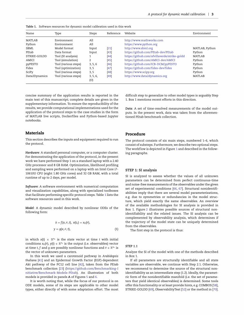
Table 1. Software resources for dynamic model calibration used in this work

Name Type Steps Reference Website Environment

MATLAB Environment All http://www.mathworks.comPython Environment All https://www.python.orgSBML Model format Input [21] http://www.sbml.org MATLAB, PythonPEtab Data format Input [43] https://github.com/PEtab-dev/PEtab PythonSTRIKE-GOLDD Tool (SI analysis) 1 [44] https://github.com/afvillaverde/strike-goldd MATLABAMICI Tool (simulation) 2 [45] https://github.com/AMICI-dev/AMICI PythonpyPESTO Tool (various steps) 3, 5, 6 [46] https://github.com/ICB-DCM/pyPESTO PythonFides Tool (optimization) 3, 5 [47] https://github.com/fides-dev/fides PythonSciPy Tool (various steps) 3, 5 [48] https://www.scipy.org PythonData2Dynamics Tool (various steps) 3, 5, 6,

(O)[49] http://www.data2dynamics.org MATLAB

concise summary of the application results is reported in themain text of this manuscript; complete details are given in thesupplementary information. To ensure the reproducibility of theresults, we provide computational implementations used for theapplication of the protocol steps to the case studies in the formof MATLAB live scripts, Dockerfiles and Python-based Jupyternotebooks.

MaterialsThis section describes the inputs and equipment required to runthe protocol.

Hardware: A standard personal computer, or a computer cluster.For demonstrating the application of the protocol, in the presentwork we have performed Step 1 on a standard laptop with a 2.40GHz processor and 8 GB RAM. Optimization, likelihood profilingand sampling were performed on a laptop with an Intel Core i7-10610U CPU (eight 1.80 GHz cores) and 32 GB RAM, with a totalruntime of up to 2 days, per model.

Software: A software environment with numerical computationand visualization capabilities, along with specialized toolboxesthat facilitate performing specific protocol steps. Table 1 lists thesoftware resources used in this work.

Model: A dynamic model described by nonlinear ODEs of thefollowing form:

x = f (x, θ , t), x(t0) = x0(θ ),

y = g(x, θ , t), (1)

in which x(t) ∈ Rnx is the state vector at time t with initial

conditions x0(θ ), y(t) ∈ Rny is the output (i.e. observables) vector

at time t, f and g are possibly nonlinear functions and θ ∈ Rnθ is

the vector of unknown parameters.In this work we used a carotenoid pathway in Arabidopsis

thaliana [41] and an Epidermal Growth Factor (EGF)-dependentAkt pathway of the PC12 cell line [42], taken from the PEtabbenchmark collection [23] (https://github.com/Benchmarking-Initiative/Benchmark-Models-PEtab). An illustration of bothmodels is provided in panels A of Figures 5 and 6.

It is worth noting that, while the focus of our protocol is onODE models, some of its steps are applicable to other modeltypes, either directly of with some adaptation effort. The most

difficult step to generalize to other model types is arguably Step1. Box 1 mentions recent efforts in this direction.

Data: A set of time-resolved measurements of the model out-puts. In the present work, data was taken from the aforemen-tioned PEtab benchmark collection.

ProcedureThe protocol consists of six main steps, numbered 1–6, whichconsist of substeps. Furthermore, we describe two optional steps.The workflow is depicted in Figure 1 and described in the follow-ing paragraphs.

STEP 1: SI analysis

SI is analyzed to assess whether the values of all unknownparameters can be determined from perfect continuous-timeand noise-free measurements of the observables under the givenset of experimental conditions [66, 67]. Structural nonidentifi-abilities imply that there are several model parameterizations,e.g. due to symmetries or redundancies in the model struc-ture, which yield exactly the same observables. An overviewof the available methodologies for SI analysis is provided inBox 1. Figure 2 illustrates possible sources of structural non-identifiability and the related issues. The SI analysis can becomplemented by observability analysis, which determines ifthe trajectory of the model state can be uniquely determinedfrom the observables.

The first step in the protocol is thus:

STEP 1.1

Analyze the SI of the model with one of the methods describedin Box 1.

If all parameters are structurally identifiable and all statevariables are observable, we continue with Step 2.1. Otherwise,we recommend to determine the source of the structural non-identifiability as an intermediate step (1.2). Ideally, the paramet-ric form of the nonidentifiable manifold (i.e. the set of parame-ters that yield identical observables) is determined. Some toolsoffer this functionality or at least provide hints, e.g. COMBOS [58],STRIKE-GOLDD [69], ObservabilityTest [52] or the method in [70].

4 Villaverde et al.

.

STEP 1.2

If parameters are structurally nonidentifiable or state variablesunobservable, use knowledge about the structure of the non-identifiable manifold to

(i) Reformulate the model by merging the nonidentifiableparameters into identifiable combinations, OR

(ii) Fix the nonidentifiable parameters to reasonable values,taken e.g. from the literature or from publicly availablebiological knowledge databases.

In both cases, the information about the nonidentifiability needsto be retained to later perform a proper analysis of the predictionuncertainties. That is, since parametric uncertainty can propa-gate to prediction uncertainty, when calculating the confidenceinterval of a prediction (STEP 6) the fixed parameters must bevaried along the range of values that was initially considered.If this point is not taken into account, the obtained confidenceintervals are only valid for the reformulated model, but not forthe original one—a fact that is often disregarded.

Model reformulation can be illustrated with the examplein Figure 2. Using the AutoRepar function in STRIKE-GOLDD, astructurally identifiable reparameterization of the mRNA trans-lation model is obtained. The new variables are M = k · s · mRNA,P = s · GFP, M0 = k · s · mRNA0. The new equations are M = −γ · M,P = −δ · P + M, y = P. Note that, while the resulting model isstructurally identifiable and observable, its variables no longerhave their original full mechanistic meaning. This is very often,but not always, the case [69]. The model user must decide ifsuch a transformation is acceptable depending on the modelpurposes. It should also be noted that it is not always possibleto find an identifiable reparameterization.

An alternative to the reformulation of the model or the fixingof parameters is to plan additional experiments, if possible.These can be experiments with new experimental conditions,new observables or both (keeping experimental constraints in

mind). The additional information should be recorded such thatmore, ideally all, parameters are structurally identifiable.

STEP 2: Formulation of objective function

The objective function measuring the mismatch of simulatedmodel observables and measurement data is defined. The choiceof the objective function depends on the characteristics of themeasurement technique and accounts for knowledge about itsaccuracy. Possible choices are discussed in Box 2.

STEP 2.1

Construct an objective function.

STEP 3: Parameter optimization

Parameter estimates are obtained by minimizing the objectivefunction. To this end, numerical optimization methods suitedfor nonlinear problems with local minima should be employed.Available methodologies and practical tips for their applicationare discussed in Box 3, and key aspects are illustrated in Fig. 3.

STEP 3.1

Launch multiple runs of local, global or hybrid optimizationalgorithms. The number of runs required is model-dependent.For an initial optimization we recommend at least 50 runs withpurely local searches or at least 10 runs with global or hybridsearches.

Accurate gradient computation is required for gradient-basedoptimization. Before optimization, check that the gradientsappear correct by evaluating the gradient at a point, andthen compare this with forward, backward and central finitedifference approximations of the gradient that are evaluatedwith different step sizes. Such a gradient check is a common,possibly optional, feature of tools that provide gradient-basedoptimization.

A protocol for dynamic model calibration 5

Figure 2. SI analysis. (A) Diagram of a simplified model of mRNA translation considering only the process in the cytosol. The model captures the translation of mRNA

and the degradation of mRNA and protein. (B) Mathematical formulation (ODEs) of mRNA translation dynamics [68] involving two states, mRNA and green fluorescent

protein (GFP). (C) The model output is the fluorescence intensity, which is proportional to the GFP level. The model has five unknown parameters: the initial condition of

the unmeasured state (mRNA0), three kinetic parameters (γ , δ, k) and an output scaling parameter(s). Given its simplicity, it is possible to calculate the output time-course

analytically (here shown for γ �= δ). The resulting function contains the product of three parameters (s·k·mRNA0), which is shown in orange, and an expression involving

δ and γ , which are shown in green. The latter expression is symmetrical with respect to δ and γ : their values can be exchanged without changing the result. Thus,

these two parameters are not structurally globally identifiable, but only locally identifiable with two possible solutions. Furthermore, the product (s · k · mRNA0) allows

for an infinite number of parameter combinations; the three involved parameters are structurally nonidentifiable. (D) Illustration of structural nonidentifiability: the

time-course of the model output is identical for an infinite number of parameter vectors. (E) Illustration of unobservability caused by nonidentifiability. For illustration

purposes, three different parameter vectors are shown, all of which produce the same model output. Each of them yields a different simulation of the mRNA time-

course; thus, this state cannot be determined. (F) Illustration of the correlations between the nonidentifiable parameters. The line indicates parameter combinations

for which the time-dependent output is identical.

STEP 3.2

Evaluate the reproducibility of the fitting results by comparingthe optimal objective function values achieved by different runs.The optimal objective function values should be robustly repro-ducible, meaning that a substantial number of runs (rule-of-thumb: 5) should find it. If this is not the case, repeat Step 3.1with a larger number of runs. Note that the difference betweenruns that is considered negligible should be statistically moti-vated. For the use of log-likelihood and log-posterior this corre-sponds to an absolute difference, not a relative one [23].

STEP 4: Goodness of fit

The quality of the fitted model should be assessed by visualinspection or use quantitative metrics. Details are provided inBox 4.

STEP 4.1

Assess the goodness of the fit achieved by the parameter opti-mization procedure.

If the fit is not good, further action is required. Proceed toSTEP 4.2.

STEP 4.2

If the fit is not good enough, check convergence of the optimiza-tion methods.

1. If there are hints that searches were stopped prematurely(e.g. error messages that indicate that local optimizationsdid not converge), go back to STEP 3: modify the settingsof the optimization algorithms (e.g. increase maximumallowed time and/or number of evaluations) and run theoptimizations again.

2. If there are no signs of a premature stop, the problem maybe that the optimal solution lies outside the initially chosenparameter bounds → go back to STEP 3: set larger parameterbounds and run the optimizations again. In fact, this actionis advisable whenever there are parameter estimates thathit the bounds, even if the fit is good. The exceptions areparameters with hard bounds, originated by physical ormathematical constraints, which should not be enlargedbeyond the meaningful limit.

3. If the actions above do not solve the issue, it may be becausethe optimization method is not well suited for the problem→ go back to STEP 3: choose a different method and run theoptimizations again.

6 Villaverde et al.

Figure 3. Parameter optimization. (A) Multi-start local optimization involves many local optimizations that are distributed within the parameter space. In systems with

multiple optima, many starts may be required to find the global optimum. Trajectories are indicated by arrows, with their initial points indicated with ‘×’. The contour

plot shows the negative log-likelihood, with darker contours indicating lesser (better) values. In all subfigures, the colours green (global) and brown (local) are used to

indicate results that correspond to a particular optimum, and parameters are labelled as θ with an index as the subscript. This subfigure is for illustration purposes only,

as it is generally infeasible to produce. (B) Convergence of starts towards an optimum can be assessed with a waterfall plot, where the existence of (multiple) plateaus

indicates optimizer convergence. If plateau(s) are not seen, possible solutions include: additional starts; alternative initial points or alternative global optimization

methods. (C) A parallel coordinates plot can be used to assess whether parameters are well determined. Here, lines belonging to a single optimum overlap (indicated

with n), suggesting that the parameters that have converged to the corresponding optimum are well determined.

If the new optimizations performed in STEP 4.2 do not yetyield a good fit, there may be a problem with the choice ofobjective function. Proceed to STEP 4.3.

STEP 4.3

If the fit is not good enough, go back to STEP 2 and select adifferent objective function.

If the new optimization results are still inappropriate, theproblem might be the model structure. Proceed to STEP 4.4.

STEP 4.4

If the fit is not good enough, go back to the model equations andperform a model refinement.

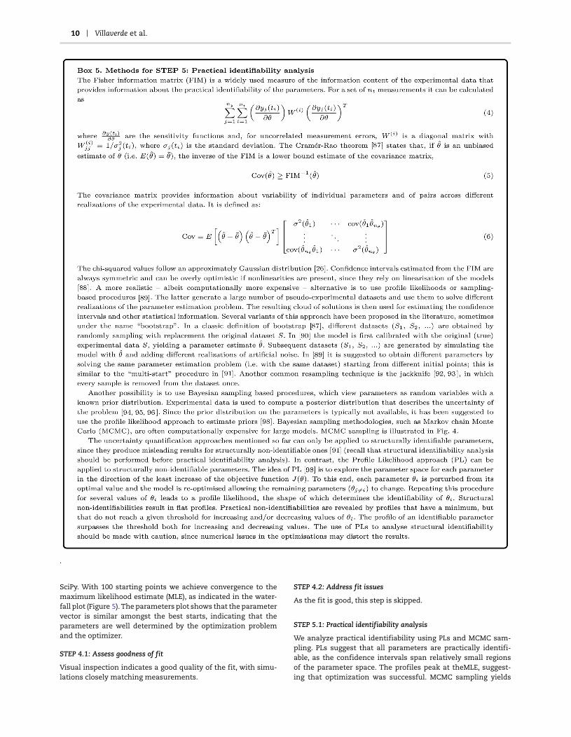
STEP 5: Practical identifiability analysis

The task of quantifying the uncertainty in parameterestimates is known as practical (or numerical) identifiabilityanalysis. It involves calculating univariate confidence intervalsor multivariate confidence regions for the parameter values.Key concepts and tools for practical identifiability analysis arelisted in Box 5. Practical identifiability issues are illustrated inFigures 5D and 6D.

STEP 5.1

Perform practical identifiability analysis with one of the meth-ods described in Box 5. If this analysis reveals uncertainties inparameter estimates that are too large for the intended applica-tion of the model, then proceed to STEP 5.2.

STEP 5.2

If there are large uncertainties, then:

1. If it is possible to perform new experiments → add moreexperimental data. In this case, the experiment should beoptimally designed in order to yield maximally informativedata. This is described in the following section.

2. If it is not possible to perform new experiments → assessthe possibility of simplifying the model parameterizationwithout losing biological interpretability.

3. If neither (1) nor (2) are possible → include prior knowledgeabout parameter values. Such information (either about thevalue of a parameter or about its bounds) can sometimes befound in publicly available databases.

After performing one of the above actions, go back to STEP 3.

(OPTIONAL STEP): Alternative experimental designfor parameter estimation

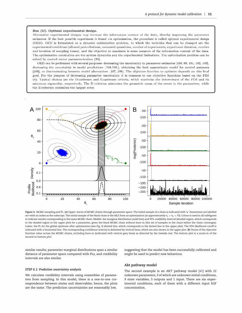
If practical identifiability analysis concludes that there are largeuncertainties in the parameter estimates, a solution may be tocollect new data. Ideally, it should be obtained by designing andperforming new experiments in an optimal way. Optimal exper-iment design (OED) seeks to maximize the information contentof the new experiments. It can be performed using optimizationtechniques that minimize an objective function that representssome measure of the uncertainty in the parameters. It is alsopossible to perform OED for other goals, such as model discrimi-nation or decreasing prediction uncertainty. OED techniques arediscussed in Box (O).

A protocol for dynamic model calibration 7

.

STEP O.1

Define the constraints of the new experimental setup and, incase of optimal design, the criterion to optimize.

STEP O.2

Obtain a new set of experiments, either by optimization or froman educated guess.

STEP O.3

Perform experiments and collect data.

STEP O.4

Include the new data in the objective function and repeat STEPS2–5.

8 Villaverde et al.

.

STEP 6: Prediction uncertainty quantification

If the calibrated model is used for making predictions, for exam-ple about the time course of its states, it is useful to assess theprediction uncertainty. This assessment is nontrivial becauseuncertainty in parameters does not directly translate to uncer-tainty in predictions. Hence, it is pertinent to quantify to whichextent the uncertainty in model parameters leads to uncertaintyin the predictions of state trajectories. Note that, if some param-eters were fixed in STEP 1 to achieve SI, in this step several valueswithin their plausible range should be considered, in order toobtain realistic confidence intervals of the state predictions. Theavailable methods for prediction uncertainty quantification arereviewed in Box 6. Their application to case studies is shown inFigures 5E and 6E.

STEP 6.1

Calculate confidence intervals for the time courses of the pre-dicted quantities of interest using one of the methods in Box6.

(OPTIONAL STEP): Model selection

The protocol presented so far assumes that the model structureis known, except for the specific values of the parameters. Some-times the form of the dynamic equations that define the model—and not only the parameter values—is not completely knowna priori, and a family of candidate models may be considered.Model selection techniques choose the best model from the setof possible ones, aiming at a balance between model complexityand goodness of fit. They are discussed in Box (MS).

A protocol for dynamic model calibration 9

.

TroubleshootingTroubleshooting advice can be found in Table 2.

ExamplesHere, we demonstrate the protocol by describing its applicationto two examples. The results described here can be reproducedwith Matlab live scripts and Jupyter notebooks, which are pro-vided as supplementary material. Additionally, pdf documentsthat show the scripts and the output generated by them are alsoincluded.

Carotenoid pathway model

Our first case study is the carotenoid pathway model by Brunoet al. [41], with 7 states, 13 parameters and no inputs. The modeloutput differs among the experimental conditions: in each ofthe six experimental conditions for which data is available, onlyone of the 7 state variables is measured (one is measured in twoexperiments, and two states are never measured).

The application of the protocol is summarized in the follow-ing paragraphs, and the main results are shown in Figure 5.

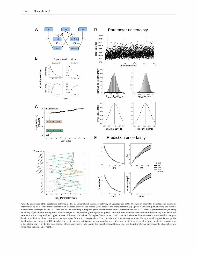
STEP 1.1: SI analysis

We first assess SI and observability for each individual exper-imental condition, obtaining a different subset of identifiableparameters for each one. Next, we repeat the analysis aftercombining the information from all experiments, obtaining thatall parameters are structurally identifiable. However, the twostate variables that are not measured in any experiment (β-ioand OH-β-io) are not observable. If the initial conditions of thesetwo states were considered as unknown parameters, they wouldbe nonidentifiable.

STEP 1.2: Address structural nonidentifiabilities

We are not interested in the two unobservable states. Hence, weomit this step and proceed with the original model.

STEP 2.1: Objective function

We use the negative log-likelihood objective function describedin Equation 2, which is the common choice in frequentistapproaches.

STEP 3.1 and 3.2: Parameter optimization

We estimate model parameters using the multi-start local opti-mization method L-BFGS-B implemented in the Python package

10 Villaverde et al.

.

SciPy. With 100 starting points we achieve convergence to themaximum likelihood estimate (MLE), as indicated in the water-fall plot (Figure 5). The parameters plot shows that the parametervector is similar amongst the best starts, indicating that theparameters are well determined by the optimization problemand the optimizer.

STEP 4.1: Assess goodness of fit

Visual inspection indicates a good quality of the fit, with simu-lations closely matching measurements.

STEP 4.2: Address fit issues

As the fit is good, this step is skipped.

STEP 5.1: Practical identifiability analysis

We analyze practical identifiability using PLs and MCMC sam-pling. PLs suggest that all parameters are practically identifi-able, as the confidence intervals span relatively small regionsof the parameter space. The profiles peak at theMLE, suggest-ing that optimization was successful. MCMC sampling yields

A protocol for dynamic model calibration 11

.

Figure 4. MCMC sampling and PL. (A) Upper: traces of MCMC chains through parameter space. The initial sample of a chain is indicated with ‘•’. Parameters are labelled

as θ with an index as the subscript. The initial sample of the black chain is the MLE from an optimization (at approximately θ1 = θ2 = 70). Colour is used in all subfigures

to indicate results corresponding to the same MCMC chain. Middle: the marginal distribution (solid line) and 95% credibility interval (shaded region, which corresponds

to the shaded region in the upper plot) for a parameter, given the black MCMC chain without burn-in (the set of samples in the chain before the chain converges).

Lower: the PL for the global optimum after optimization (see Fig. 3) (dotted line, which corresponds to the dotted line in the upper plot). The 95% likelihood cutoff is

indicated with a horizontal line. The corresponding confidence interval is delimited by vertical lines, which are also shown in the upper plot. (B) Traces of the objective

function value across the MCMC chains, including burn-in (indicated with vertical grey lines) as detected by the Geweke test. The bottom plot is a zoom-in of the

second-to-bottom plot.

similar results; parameter marginal distributions span a similardistance of parameter space compared with PLs, and credibilityintervals are also similar.

STEP 6.1: Prediction uncertainty analysis

We calculate credibility intervals using ensembles of parame-ters from sampling. In this model, there is a one-to-one cor-respondence between states and observables; hence, the plotsare the same. The prediction uncertainties are reasonably low,

suggesting that the model has been successfully calibrated andmight be used to predict new behaviour.

Akt pathway model

The second example is an AKT pathway model [42] with 22unknown parameters, 3 of which are unknown initial conditions,9 state variables, 3 outputs and 1 input. There are six exper-imental conditions, each of them with a different input EGFconcentration.

12 Villaverde et al.

.

.

Results are summarized in the following paragraphs and inFigure 6.

STEP 1.1: SI analysis

We consider the following scenarios:

1. For a single experiment with constant EGF, 11 parametersare structurally nonidentifiable, and 3 states are unobserv-able.

2. For a single experiment with time-varying EGF, the modelbecomes structurally identifiable and observable.

3. For multiple experiments (at least two) with constant EGF,the model is structurally identifiable and observable.

The experimental data available correspond to the scenario (3)above. The scenario (2) yields an identifiable and observablemodel, but it requires a continuously varying value of EGF, whichis not practical. It is also interesting to note the role of initialconditions in this case study. The results summarized above

A protocol for dynamic model calibration 13

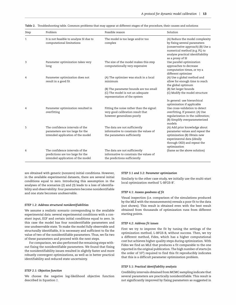
Table 2. Troubleshooting table. Common problems that may appear at different stages of the procedure, their causes and solutions

Step Problem Possible reason Solution

1 It is not feasible to analyze SI due tocomputational limitations

The model is too large and/or toocomplex

(A) Reduce the model complexityby fixing several parameters(conservative approach) (B) Use anumerical method (e.g. PL) toanalyze practical identifiabilityas a proxy of SI

3 Parameter optimization takes verylong

The size of the model makes this stepcomputationally very expensive

Use parallel optimizationapproaches to decreasecomputation times, or try adifferent optimizer

4 Parameter optimization does notresult in a good fit

(A) The optimizer was stuck in a localminimum

(A) Use a global method andallow for enough time to reachthe global optimum

(B) The parameter bounds are too small (B) Set larger bounds(C) The model is not an adequaterepresentation of the system

(C) Modify the model structure

In general: use hierarchicaloptimization if applicable

4 Parameter optimization resulted inoverfitting

Fitting the noise rather than the signal:very good calibration result thathowever generalizes poorly

Use cross-validation to detectoverfitting. If present: (A) Useregularization in the calibration;(B) Simplify overparameterizedmodels

5 The confidence intervals of theparameters are too large for theintended application of the model

The data are not sufficientlyinformative to constrain the values ofthe parameters sufficiently

(A) Add prior knowledge aboutparameter values and repeat theoptimization (B) Obtain newexperimental data (ideallythrough OED) and repeat theoptimization

6 The confidence intervals of thepredictions are too large for theintended application of the model

The data are not sufficientlyinformative to constrain the values ofthe predictions sufficiently

(Same as the above solution)

are obtained with generic (nonzero) initial conditions. However,in the available experimental datasets, there are several initialconditions equal to zero. Introducing this assumption in theanalyses of the scenarios (2) and (3) leads to a loss of identifia-bility and observability: four parameters become nonidentifiableand one state becomes unobservable.

STEP 1.2: Address structural nonidentifiabilities

We assume a realistic scenario corresponding to the availableexperimental data: several experimental conditions with a con-stant input, EGF and certain initial conditions equal to zero. Inthis case the model has four nonidentifiable parameters andone unobservable state. To make the model fully observable andstructurally identifiable, it is necessary and sufficient to fix thevalue of two of the nonidentifiable parameters. Thus, we fix twoof these parameters and proceed with the next steps.

For comparison, we also performed the remaining steps with-out fixing the nonidentifiable parameters. We found that fixingthe nonidentifiability issues resulted in slightly faster and morerobustly convergent optimizations, as well as in better practicalidentifiability and reduced state uncertainty.

STEP 2.1: Objective function

We choose the negative log-likelihood objective functiondescribed in Equation 2.

STEP 3.1 and 3.2: Parameter optimization

Similarly to the other case study, we initially use the multi-startlocal optimization method ‘L-BFGS-B’.

STEP 4.1: Assess goodness of fit

Visual inspection (i.e. comparison of the simulations producedby the MLE with the measurements) reveals a poor fit to the data(not shown). This result is obtained even with the best resultobtained from thousands of optimization runs from differentstarting points.

STEP 4.2: Address fit issues

First we try to improve the fit by tuning the settings of theoptimization method, L-BFGS-B, without success. Then, we trya different method, Fides, which has a higher computationalcost but achieves higher quality steps during optimization. WithFides we find an MLE that produces a fit comparable to the onereported in the original publication. The high number of starts (inthe order of 103) required to find this fit reproducibly indicatesthat this is a difficult parameter optimization problem.

STEP 5.1: Practical identifiability analysis

Credibility intervals obtained from MCMC sampling indicate thatseveral parameters are practically nonidentifiable. This result isnot significantly improved by fixing parameters as suggested in

14 Villaverde et al.

Figure 5. Calibration of the carotenoid pathway model. (A) Schematic of the model pathway. (B) Visualization of the fit. The plot shows the trajectories of the model

observables, as well as the means (points) and standard errors of the means (error bars) of the measurements. (C) Upper: A waterfall plot, showing the number

of starts that converged to the MLE. Here and in the remaining subfigures, green indicates results that correspond to the MLE. Lower: A parameters plot, showing

variability of parameters among starts that converged to the possible global optimum (green). Vertical dotted lines indicate parameter bounds. (D) Plots related to

parameter uncertainty analysis. Upper: a trace of the function values of samples from a MCMC chain. The vertical dotted line indicates burn-in. Middle: marginal

density distributions of two parameters, using samples from the converged chain. The plots show a kernel density estimate, histogram and rug plot. Lower: profile

likelihood of two parameters. (E) Plots related to prediction uncertainty analysis, computed as percentiles from predictions of samples. Upper: prediction uncertainties

of two states. Lower: prediction uncertainties of two observables. Note that in this model, observables are states without transformation; hence, the observables and

states have the same uncertainties.

A protocol for dynamic model calibration 15

Figure 6. Calibration of the Akt pathway model. (A) Schematic of the model pathway. (B) Visualization of the fit. The plot shows the trajectories of the model observables,

as well as the means (points) and standard errors of the means (error bars) of the measurements. (C) Upper: A waterfall plot, showing the number of starts that converged

to the MLE. Here and in the remaining subfigures, green indicates results that correspond to the MLE. Lower: A parameters plot, showing variability of parameters among

starts that converged to the possible global optimum (green). Vertical dotted lines indicate parameter bounds. (D) Plots related to parameter uncertainty analysis. Upper:

a trace of the function values of samples from an MCMC chain. The vertical dotted line indicates burn-in. Middle: marginal density distributions for two parameters,

using samples from the converged chain. The plots show a kernel density estimate, histogram and rug plot. Lower: profile likelihood of two parameters. The dotted

vertical line indicates a parameter bound. (E) Plots related to prediction uncertainty analysis, computed as percentiles from predictions of samples. Upper: prediction

uncertainties of two states under one experimental condition. Lower: prediction uncertainties of two observables under one experimental condition.

16 Villaverde et al.

STEP 1.2. Improving the practical identifiability of these param-eters would require repeating the calibration with additionalexperimental data.

STEP 6.1: Prediction uncertainty analysis

Credibility intervals obtained from MCMC sampling indicate thatthe uncertainties in the observable trajectories are reasonablylow. However, the state trajectories have larger uncertainties,which make this calibrated model unsuitable for predictionsinvolving these states. The quality of the predictions can beimproved by reducing practical nonidentifiabilities in the model,as mentioned in the previous step.

Discussion and conclusionIn this paper, we have proposed a pipeline of methods andresources for calibrating ODE models in the context of bio-logical applications. Its end goal is to obtain a model that iscapable of making predictions about quantities of interest withquantifiable uncertainty.

The pipeline consists of a series of steps, each of whichrepresents a task that should be fulfilled before proceeding tothe next one to ensure a successful calibration. Performing thesetasks entails applying computational methods of different types,symbolic and numerical. The analyses and calculations can becomputationally challenging in practice. While the protocol isnot dependent on a particular choice of software, we have rec-ommended a number of state-of-the-art tools that implementthe methods.

To facilitate the application of the protocol by novices as wellas by experienced modellers, we have described in detail how toperform each of the protocol steps. We have also provided thetheoretical background required for understanding the under-lying problems. Furthermore, we have illustrated its use withtwo case studies: a carotenoid pathway model in A. thaliana andan EGF-dependent Akt pathway of the PC12 cell line. Finally, wehave highlighted some of the most common pitfalls in biologicalmodelling, showing how to avoid them.

Key Points• The correct calibration of dynamic models is essential

for obtaining correct predictions and insights.• While a wide range of tools and resources are cur-

rently available, there are also many potential pitfalls,even for the expert.

• Here we propose a model calibration protocol thatcovers all aspects of the problem.

• The present paper guides the user through all thesteps of the pipeline, providing a one-stop guide thatis at the same time compact and comprehensive.

• We provide all the code required to reproduce theresults and perform the same analysis on new mod-els, so that the biological modelling community canbenefit from this pipeline.

Supplementary data

All data, scripts and examples presented in this paper canbe downloaded from https://github.com/ICB-DCM/model_calibration_protocol. Supplementary data are also availableonline at https://academic.oup.com/bib.

Funding

European Union’s Horizon 2020 Research and InnovationProgramme (grant no. 686282) (‘CANPATHPRO’); Span-ish MINECO/FEDER Project SYNBIOCONTROL (DPI2017-82896-C2-2-R to J.R.B.); Ramón y Cajal Fellowship (RYC-2019-027537-I to A.F.V.) from the Ministerio de Ciencia einnovación, Spain; Consellería de Cultura, Educación eOrdenación Universitaria, Xunta de Galicia (ED431F 2021/003to A.F.V.); Deutsche Forschungsgemeinschaft (DFG, GermanResearch Foundation) under Germany’s Excellence Strategy(EXC 2151 - 390873048 to J.H.), (EXC-2047/1 - 390685813to D.P.); German Federal Ministry of Economic Affairsand Energy (grant no. 16KN074236 to D.P.). Ministerio deCiencia e Innovación, Spain (grant PID2020-117271RB-C22,‘BIODYNAMICS’, to J.R.B.; Funding for open access charge:Universidade de Vigo/CISUG).

References1. Kuepfer L, Peter M, Sauer U, et al. Ensemble modeling

for analysis of cell signaling dynamics. Nat Biotechnol2007;25(9):1001–6.

2. Sachs K, Itani S, Fitzgerald J, et al. Learning cyclic signalingpathway structures while minimizing data requirements.In: Pacific Symposium on Biocomputing. Pacific Symposium onBiocomputing. NIH Public Access, Kohala Coast, Hawaii, USA,2009, 63.

3. Fröhlich F, Kessler T, Weindl D, et al. Efficient parame-ter estimation enables the prediction of drug responseusing a mechanistic pan-cancer pathway model. Cell Syst2018;7(6):567–79.

4. Henriques D, Villaverde AF, Rocha M, et al. Data-driven reverse engineering of signaling pathwaysusing ensembles of dynamic models. PLoS Comput Biol2017;13(2):e1005379.

5. Song H-S, DeVilbiss F, Ramkrishna D. Modeling metabolicsystems: the need for dynamics. Curr Opin Chem Eng2013;2(4):373–82.

6. Almquist J, Cvijovic M, Hatzimanikatis V, et al. Kineticmodels in industrial biotechnology–improving cell factoryperformance. Metab Eng 2014;24:38–60.

7. Villaverde AF, Bongard S, Mauch K, et al. Metabolic engineer-ing with multi-objective optimization of kinetic models. JBiotechnol 2016;222:1–8.

8. Briat C, Khammash M. Perfect adaptation and optimalequilibrium productivity in a simple microbial biofuelmetabolic pathway using dynamic integral control. ACSSynth Biol 2018;7(2):419–31.

9. Karamasioti E, Lormeau C, Stelling J. Computational designof biological circuits: putting parts into context. Mol SystDesign Eng 2017;2(4):410–21.

10. Hsiao V, Swaminathan A, Murray RM. Control theory forsynthetic biology: recent advances in system characteri-zation, control design, and controller implementation forsynthetic biology. IEEE Control Syst 2018;38(3):32–62.

11. Steel H, Papachristodoulou A. Design constraints for bio-logical systems that achieve adaptation and disturbancerejection. IEEE Trans Control Netw Syst 2018;5(2):807–17.

12. Tomazou M, Barahona M, Polizzi KM, et al. Computa-tional re-design of synthetic genetic oscillators for inde-pendent amplitude and frequency modulation. Cell Syst2018;6(4):508–20.

A protocol for dynamic model calibration 17

13. Kanehisa M, Goto S. Kegg: kyoto encyclopedia of genes andgenomes. Nucleic Acids Res 2000;28(1):27–30.

14. Szklarczyk D, Morris JH, Cook H, et al. The stringdatabase in 2017: quality-controlled protein–proteinassociation networks, made broadly accessible. NucleicAcids Res 2016;45:gkw937.

15. Fabregat A, Jupe S, Matthews L, et al. The reactome pathwayknowledgebase. Nucleic Acids Res 2017;46(D1):D649–55.

16. Olivier BG, Snoep JL. Web-based kinetic modelling usingJWS online. Bioinformatics 2004;20(13):2143–4.

17. Le Novère N, Bornstein B, Broicher A, et al. BioModelsdatabase: a free, centralized database of curated, published,quantitative kinetic models of biochemical and cellularsystems. Nucleic Acids Res Jan 2006;34(database issue):D689–91.

18. Chang A, Schomburg I, Placzek S, et al. Brenda in 2015:exciting developments in its 25th year of existence. NucleicAcids Res 2014;43:gku1068.

19. Wittig U, Kania R, Golebiewski M, et al. Sabio-rk databasefor biochemical reaction kinetics. Nucleic Acids Res2012;40(D1):D790–6.

20. van Riel NAW. Dynamic modelling and analysis ofbiochemical networks: mechanism-based models andmodel-based experiments. Brief Bioinform 2006;7(4):364–74.

21. Hucka M, Finney A, Sauro HM, et al. The systems biologymarkup language (SBML): a medium for representation andexchange of biochemical network models. Bioinformatics2003;19:524–31.

22. Villaverde AF, Fröhlich F, Weindl D, et al. Benchmarkingoptimization methods for parameter estimation in largekinetic models. Bioinformatics 2018;35(5):830–8.

23. Hass H, Loos C, Raimúndez-Álvarez E, et al. Benchmarkproblems for dynamic modeling of intracellular processes.Bioinformatics 2019;35(17):3073–82.

24. Jaqaman K, Danuser G. Linking data to models: data regres-sion. Nat Rev Mol Cell Bio 2006;7(11):813–9.

25. Ashyraliyev M, Fomekong-Nanfack Y, Kaandorp JA, et al.Systems biology: parameter estimation for biochemicalmodels. FEBS J 2009;276(4):886–902.

26. Geier F, Fengos G, Felizzi F, et al. Analyzing and constrainingsignaling networks: parameter estimation for the user. In:Liu X, Betterton MD (eds). Computational Modeling of SignalingNetworks, Volume 880 of Methods in Molecular Biology. Totowa,NJ: Humana Press, 2012, 23–40.

27. Raue A, Schilling M, Bachmann J, et al. Lessons learned fromquantitative dynamical modeling in systems biology. PLoSOne Jan 2013;8(9):e74335.

28. Kapil G, Kirouac DC, Mager DE, et al. A six-stage work-flow for robust application of systems pharmacology. CPTPharmacometrics Syst Pharmacol 2016;5(5):235–49.

29. Villaverde AF, Banga JR. Reverse engineering and identi-fication in systems biology: strategies, perspectives andchallenges. J R Soc Interface 2014;11(91):20130505.

30. Schoukens J, Ljung L. Nonlinear system identification: auser-oriented road map. IEEE Control Syst Mag 2019;39(6):28–99.

31. Balsa-Canto E, Alonso AA, Banga JR. An iterative identi-fication procedure for dynamic modeling of biochemicalnetworks. BMC Syst Biol 2010;4:11.

32. Seaton DD. ODE-Based Modeling of Complex Regulatory Cir-cuits. New York, NY: Springer New York, 2017, 317–30.

33. Eisenkolb I, Jensch A, Eisenkolb K, et al. Modeling ofbiocatalytic reactions: a workflow for model calibration,

selection and validation using Bayesian statistics. AIChE Jl2019;66(4):e16866.

34. Mannina G, Cosenza A, Vanrolleghem PA, et al. A practicalprotocol for calibration of nutrient removal wastewatertreatment models. J Hydroinf 2011;13(4):575–95.

35. Zhu A, Guo J, Ni B-J, et al. A novel protocol for model calibra-tion in biological wastewater treatment. Sci Rep 2015;5:8493.

36. Vilas C, Arias-Méndez A, García MR, et al. Toward predictivefood process models: a protocol for parameter estimation.Crit Rev Food Sci Nutr 2018;58(3):436–49.

37. Tuza Z, Bandiera L, Gomez-Cabeza D, et al. A systematicframework for biomolecular system identification. In: Pro-ceedings of the 58th IEEE Conference on Decision and Control,2019. IEEE, Nice, France.

38. Whittaker DG, Clerx M, Lei CL, et al. Calibration of ionic andcellular cardiac electrophysiology models. Wiley InterdiscipRev Syst Biol Med 2020;12(4):e1482.

39. Steiert B, Kreutz C, Raue A, et al. Recipes for analysisof molecular networks using the Data2Dynamics model-ing environment. In: Modeling Biomolecular Site Dynamics.Springer, Cham, Switzerland, 2019, 341–62.

40. Raue A, Steiert B, Schelker M, et al. Data2dynamics:a modeling environment tailored to parameter estima-tion in dynamical systems. Bioinformatics 2015;31(21):3558–60.

41. Bruno M, Koschmieder J, Wuest F, et al. Enzymatic studyon atccd4 and atccd7 and their potential to form acyclicregulatory metabolites. J Exp Bot 2016;67(21):5993–6005.

42. Fujita KA, Toyoshima Y, Uda S, et al. Decoupling of receptorand downstream signals in the Akt pathway by its low-passfilter characteristics. Sci Signal 2010;3(132):ra56–6.

43. Schmiester L, Schälte Y, Bergmann FT, et al. Petab-interoperable specification of parameter estimation prob-lems in systems biology. PLoS Comput Biol 2021;17(1):e1008646.

44. Villaverde AF, Tsiantis N, Banga JR. Full observabilityand estimation of unknown inputs, states and param-eters of nonlinear biological models. J R Soc Interface2019;16(156):20190043.

45. Fröhlich F, Kaltenbacher B, Theis FJ, et al. Scalable parame-ter estimation for genome-scale biochemical reaction net-works. PLoS Comput Biol 2017;13(1):e1005331.

46. Stapor P, Weindl D, Ballnus B, et al. Pesto: parameter esti-mation toolbox. Bioinformatics 2017;34(4):705–7.

47. Froehlich F, Sorger PK. Fides: Reliable trust-region opti-mization for parameter estimation of ordinary differentialequation models. bioRxiv 2021; 2021.05.20.445065.

48. Virtanen P, Gommers R, Oliphant TE, et al. SciPy 1.0: funda-mental algorithms for scientific computing in Python. NatMethods 2020;17:261–72.

49. Miao H, Xia X, Perelson AS, et al. On identifiability of non-linear ode models and applications in viral dynamics. SIAMRev Soc Ind Appl Math 2011;53(1):3–39.

50. Chis O, Banga JR, Balsa-Canto E. Structural identifiability ofsystems biology models: a critical comparison of methods.PLoS One 2011;6(11):e27755.

51. Villaverde AF. Observability and structural identi-fiability of nonlinear biological systems. Complexity2019;2019:8497093.

52. Sedoglavic A. A probabilistic algorithm to test local alge-braic observability in polynomial time. J Symbolic Comput2002;33(5):735–55.

53. Karlsson J, Anguelova M, Jirstrand M. An efficient methodfor structural identiability analysis of large dynamic

18 Villaverde et al.

systems. In: 16th IFAC Symposium on System Identification,IFAC, Brussels, Belgium. Vol. 16, 2012, 941–6.

54. Ohtsuka T. Model structure simplification of nonlin-ear systems via immersion. IEEE Trans Automatic Control2005;50(5):607–18.

55. Chatzis MN, Chatzi EN, Smyth AW. On the observabilityand identifiability of nonlinear structural and mechanicalsystems. Struct Control Health Monit 2015;22(3):574–93.

56. Ligon TS, Fröhlich F, Chis OT, et al. Genssi 2.0: multi-experiment structural identifiability analysis of sbml mod-els. Bioinformatics 2017;34(8):1421–3.

57. Hong H, Ovchinnikov A, Pogudin G, et al. Sian: software forstructural identifiability analysis of ode models. Bioinfor-matics 2019;35(16):2873–4.

58. Meshkat N, Kuo CE, DiStefano JIII. On finding and usingidentifiable parameter combinations in nonlinear dynamicsystems biology models and combos: a novel web imple-mentation. PLoS One 2014;9(10):e110261.

59. Saccomani MP, Bellu G, Audoly S, et al. A new version ofdaisy to test structural identifiability of biological mod-els. In: International Conference on Computational Methods inSystems Biology. Springer, Cham, Switzerland, 2019, 329–34.

60. Stigter JD, Molenaar J. A fast algorithm to assess localstructural identifiability. Automatica 2015;58:118–24.

61. Alkhoury Z, Petreczky M, Mercère G. Identifiability of affinelinear parameter-varying models. Automatica 2017;80:62–74.

62. Anstett F, Bloch G, Millérioux G, et al. Identifiability ofdiscrete-time nonlinear systems: the local state isomor-phism approach. Automatica 2008;44(11):2884–9.

63. Nõmm S, Moog CH. Further results on identifiability ofdiscrete-time nonlinear systems. Automatica 2016;68:69–74.

64. Browning AP, Warne DJ, Burrage K, et al. Identifiability anal-ysis for stochastic differential equation models in systemsbiology. J R Soc Interface 2020;17(173):20200652.

65. Renardy M, Kirschner D, Eisenberg M. Structural iden-tifiability analysis of pdes: a case study in contin-uous age-structured epidemic models. arXiv preprintarXiv:2102.06178. 2021.

66. Walter E, Pronzato L. Identification of Parametric Models fromExperimental Data. Masson: Springer, 1997.

67. DiStefano JIII. Dynamic Systems Biology Modeling and Sim-ulation. Academic Press, Cambridge, Massachusetts, USA,2015.

68. Ballnus B, Schaper S, Theis FJ, et al. Bayesian parame-ter estimation for biochemical reaction networks usingregion-based adaptive parallel tempering. Bioinformatics2018;34(13):i494–501.

69. Massonis G, Banga JR, Villaverde AF. Repairing dynamicmodels: a method to obtain identifiable and observ-able reparameterizations with mechanistic insights. arXivpreprint arXiv:2012.09826. 2020.

70. Merkt B, Timmer J, Kaschek D. Higher-order lie symmetriesin identifiability and predictability analysis of dynamicmodels. Phy Rev E 2015;92(1):012920.

71. Hengl S, Kreutz D, Timmer J, et al. Data-based identifiabil-ity analysis of non-linear dynamical models. Bioinformatics2007;23(19):2612–8.

72. Maier A, Westphal S, Geimer T, et al. Fast pose verificationfor high-speed radiation therapy. In: Bildverarbeitung für dieMedizin 2017. Springer, Cham, Switzerland, 2017, 104–9.

73. Mitra ED, Dias R, Posner RG, et al. Using both qualitative andquantitative data in parameter identification for systemsbiology models. Nat Commun 2018;9(1):1–8.

74. Mitra ED, Hlavacek WS. Bayesian inference using qual-itative observations of underlying continuous variables.Bioinformatics 2020;36(10):3177–84.

75. Schmiester L, Weindl D, Hasenauer J. Parameterizationof mechanistic models from qualitative data using anefficient optimal scaling approach. J Math Biol2020;81(2):603–23.

76. Schmiester L, Weindl D, Hasenauer J. Efficient gradient-based parameter estimation for dynamic models usingqualitative data. Bioinformatics 2021;btab512.

77. Hadamard J. Sur les problèmes aux dérivées partielles etleur signification physique. Princeton Univ Bull 1902;13:49–52.

78. Lopez D, Barz T, Körkel S, et al. Nonlinear ill-posed prob-lem analysis in model-based parameter estimation andexperimental design. Comput Chem Eng 2015;77:24–42.

79. Hross S, Hasenauer J. Analysis of CFSE time-series datausing division-, age-and label-structured population mod-els. Bioinformatics 2016;32(15):2321–9.

80. Kreutz C. New concepts for evaluating the performance ofcomputational methods. IFAC-Papers OnLine 2016;49(26):63–70.

81. Loos C, Krause S, Hasenauer J. Hierarchical optimization forthe efficient parametrization of ode models. Bioinformatics2018;34(24):4266–73.

82. Schmiester L, Schälte Y, Fröhlich F, et al. Efficient parame-terization of large-scale dynamic models based on relativemeasurements. Bioinformatics 2020;36(2):594–602.

83. Penas DR, González P, Egea JA, et al. Parameter estima-tion in large-scale systems biology models: a paralleland self-adaptive cooperative strategy. BMC Bioinformatics2017;18(1):52.

84. Li J. Assessing the accuracy of predictive models for numer-ical data: Not r nor r2, why not? then what? PLoS One Aug2017;12(8):e0183250.

85. Efron B, Tibshirani R. Bootstrap methods for standarderrors, confidence intervals, and other measures of statis-tical accuracy. Stat Sci 1986;1(1):54–75.

86. Pillonetto G, Dinuzzo F, Chen T, et al. Kernel methodsin system identification, machine learning and functionestimation: a survey. Automatica 2014;50(3):657–82.

87. Cramér H. Mathematical Methods of Statistics (PMS-9), Vol.9. Princeton university press, Princeton, New Jersey, USA,2016.

88. Wieland F-G, Hauber AL, Rosenblatt M, et al. On structuraland practical identifiability. Curr Opin Syst Biol 2021;25:60–9.

89. Banga JR, Balsa-Canto E. Parameter estimation and optimalexperimental design. Essays Biochem 2008;45:195–210.

90. Joshi M, Seidel-Morgenstern A, Kremling A. Exploiting thebootstrap method for quantifying parameter confidenceintervals in dynamical systems. Metab Eng 2006;8:447–55.

91. Fröhlich F, Theis FJ, Hasenauer J. Uncertainty analysis fornon-identifiable dynamical systems: profile likelihoods,bootstrapping and more. In: International Conference onComputational Methods in Systems Biology. Springer, Cham,Switzerland, 2014, 61–72.

92. Tukey JW. Bias and confidence in not-quite large samples.Ann Math Statist 1958;29:614.

93. Efron B, Stein C. The Jackknife estimate of variance. Ann Stat1981;9(3):586–96.

94. Toni T, Welch D, Strelkowa N, et al. Approximate Bayesiancomputation scheme for parameter inference andmodel selection in dynamical systems. J R Soc Interface2009;6(31):187–202.

A protocol for dynamic model calibration 19

95. Liepe J, Kirk P, Filippi S, et al. A framework for parameterestimation and model selection from experimental data insystems biology using approximate Bayesian computation.Nat Protoc 2014;9(2):439–56.

96. Hug S, Raue A, Hasenauer J, et al. High-dimensionalBayesian parameter estimation: case study for a model ofjak2/stat5 signaling. Math Biosci 2013;246(2):293–304.

97. Vanlier J, Tiemann CA, Hilbers PAJ, et al. An integratedstrategy for prediction uncertainty analysis. Bioinformatics2012;28(8):1130–5.

98. Raue A, Kreutz C, Maiwald T, et al. Structural and practi-cal identifiability analysis of partially observed dynamicalmodels by exploiting the profile likelihood. BioinformaticsAug 2009;25(15):1923–9.

99. Balsa-Canto E, Alonso AA, Banga JR. Computational pro-cedures for optimal experimental design in biological sys-tems. IET Syst Biol 2008;2(4):163–72.

100. Steiert B, Raue A, Timmer J, et al. Experimental design forparameter estimation of gene regulatory networks. PLoSOne 2012;7(7):e40052.

101. Bock HG, Körkel S, Schlöder JP. Parameter estimationand optimum experimental design for differential equa-tion models. In: Model Based Parameter Estimation. Springer,Berlin, Heidelberg, 2013, 1–30.

102. Franceschini G, Macchietto S. Model-based design of exper-iments for parameter precision: state of the art. Chem EngSci 2008;63(19):4846–72.

103. Pronzato L. Optimal experimental design and some relatedcontrol problems. Automatica 2008;44(2):303–25.

104. Kreutz C, Raue A, Kaschek D, et al. Profile likelihood insystems biology. FEBS J 2013;280(11):2564–71.

105. Hagen DR, White JK, Tidor B. Convergence in parametersand predictions using computational experimental design.Interface Focus 2013;3(4):20130008.

106. Gevers M. Identification for control: from the early achieve-ments to the revival of experiment design. Eur J Control2005;11(4–5):335–52.

107. Casey FP, Baird D, Feng Q, et al. Optimal experimentaldesign in an epidermal growth factor receptor signalling

and down-regulation model. IET Syst Biol 2007;1(3):190–202.108. Waldron C, Pankajakshan A, Quaglio M, et al. Closed-

loop model-based design of experiments for kinetic modeldiscrimination and parameter estimation: benzoic acidesterification on a heterogeneous catalyst. Ind Eng Chem Res2019;58(49):22165–22177.

109. Villaverde AF, Raimúndez E, Hasenauer J, et al. A com-parison of methods for quantifying prediction uncer-tainty in systems biology. IFAC-Papers OnLine 2019;52(26):45–51.

110. Shahmohammadi A, McAuley KB. Sequential model-based a-optimal design of experiments when the fisherinformation matrix is noninvertible. Ind Eng Chem Res2019;58(3):1244–61.

111. Kreutz C, Raue A, Timmer J. Likelihood basedobservability analysis and confidence intervals forpredictions of dynamic models. BMC Syst Biol 2012;6(1):120.

112. Hass H, Kreutz C, Timmer J, et al. Fast integration-basedprediction bands for ordinary differential equation models.Bioinformatics 2015;32(8):1204–10.

113. Brown KS, Hill CC, Calero GA, et al. The statistical mechan-ics of complex signaling networks: nerve growth factorsignaling. Phys Biol 2004;1(3):184.

114. Villaverde AF, Bongard S, Mauch K, et al. A consen-sus approach for estimating the predictive accuracy ofdynamic models in biology. Comput Methods ProgramsBiomed 2015;119(1):17–28.

115. Bozdogan H. Model selection and Akaike’s information cri-terion (AIC): the general theory and its analytical exten-sions. Psychometrika 1987;52(3):345–70.

116. Vyshemirsky V, Girolami MA. Bayesian ranking ofbiochemical system models. Bioinformatics 2008;24(6):833–9.

117. Tibshirani R. Regression shrinkage and selection via theLASSO. J R Stat Soc B Methodol 1996;58(1):267–88.

118. Steiert B, Timmer J, Kreutz C. L 1 regularization facilitatesdetection of cell type-specific parameters in dynamicalsystems. Bioinformatics 2016;32(17):i718–26.