A prospect theory model of goal behavior

George Wu*

Chip Heath†

Richard Larrick‡

April 22, 2008

Goals have a powerful effect on performance: higher goals typically produce better performance. Previous research has proposed three key mechanisms to explain these results: effort, persistence, and attention. We present a formal model that relates these mechanisms to a single underlying process. Our model assumes that goals divide performance into two regions, gains and losses, and that the resulting gains and losses are coded according to a prospect theory value function (Kahneman & Tversky, 1979). This simple model explains the stylized findings in the goal setting literature, while also offering several new testable predictions.

* Graduate School of Business, University of Chicago, george.wu@gsb.uchicago.edu † Graduate School of Business, Stanford University, heath_chip@gsb.stanford.edu ‡ Fuqua School of Business, Duke University, larrick@duke.edu

Much research on goal setting has shown that higher goals tend to lead to higher

performance (see, Locke & Latham, 1990, for a review). These consistent findings have been

explained as arising from three underlying mechanisms: goals encourage individuals to expend

more effort, persist longer, and direct attention to the goal at the expense of other activities. We

show how these three mechanisms—effort, persistence, and attention—can be understood as

outcomes of a single underlying process. We model the effect of goals on performance by

positing that goals divide the world into losses and gains as described by the prospect theory

value function (Kahneman & Tversky, 1979). In doing so, our model integrates the three

underlying mechanisms proposed by previous researchers and offers some new testable

implications.

This paper provides a formal model for Heath, Larrick, & Wu’s (1999) “goals as

reference points” approach. Heath et al. showed how the major results in the goal setting

literature can be explained by an approach in which goals inherit the properties of the prospect

theory value function. That paper also developed and tested some new predictions of the value

function on goal behavior, including implications of reference-dependence, loss aversion, and

diminishing sensitivity.

Our paper is organized as follows. In Section 1, we present a brief review of the goal

setting literature, in particular the three mechanisms proposed by Locke & Latham (1990)—

effort, persistence, and attention. In Section 2, we present our prospect theory model of goal

behavior and show how effort and persistence can be interpreted within this framework. In

Section 3, we show how our model explains the final mechanism, attention. We then develop

some new implications of our model. In Section 4, we discuss the relationship between loss

aversion and “piling up”, the tendency of performance to exceed moderately challenging goals

2

by a small amount. In Section 5, we discuss how the beneficial effects of subgoaling can be

interpreted in terms of the value function. We conclude in Section 6.

1. Literature

In many areas in psychology, key theoretical results are demonstrated by a handful of

studies. The literature on goals is exceptional in that its key findings have been replicated so

many times in so many domains. “Goal setting studies have been conducted with 88 different

tasks including bargaining, driving, faculty research, health promoting behaviors, logging,

maintenance and technical work, managerial work, management training, and safety.” (Locke &

Latham, 1991, p. 212). A decade ago when Locke and Latham (1990) conducted their

comprehensive book-length review, researchers had conducted 239 laboratory and 156 field

studies involving over 40,000 people; the number has increased since then.

The most frequently researched topic in the goal literature is how the content of goals

affects performance. Research has typically found that people perform better when they are

given goals that are specific and difficult. Mento, Steel, & Karren (1987) suggested that “If there

is ever to be a viable candidate from the organizational sciences for elevation to the lofty status

of a scientific law of nature, then the relationships between goal difficulty, difficulty / specificity,

and task performance are most worthy of serious consideration” (p. 74).

For a number of years, the goal literature focused only on documenting the fact that goal

difficulty and specificity affected performance in predictable ways (Naylor & Ilgen, 1984).

More recently, researchers have spent time trying to understand why goals work as they do. The

most widely cited explanation of the performance results is that of Locke & Latham (1990, 1991)

who attribute these findings to a small number of “mediators or causal mechanisms” that are

“relatively direct and automatic consequences of goal-directed activity” (Locke & Latham, 1991,

3

p. 227). Below, we review the three mechanisms proposed by Locke and Latham (1990)—

effort, persistence, and attention. While we applaud their focus on mechanisms in a literature

that has historically not focused much on explaining its own robust empirical results (e.g., see the

critique of Naylor & Ilgen, 1984), we propose that the mechanisms explained by Locke and

Latham can themselves be explained at a deeper level as arising from a single underlying

process. In the remainder of the paper, we propose a prospect theory model of goal behavior that

explains and integrates Locke and Latham’s three “separate” mechanisms.§

Goals Increase Effort

First, Locke & Latham (1990) have argued that goals increase “effort or energy

expenditure (i.e., intensity)...” They propose that “(t)his is the core explanation of the goal

difficulty effect” (p. 227). A wide variety of experiments have demonstrated that goals increase

effort. On physical tasks, goal subjects exercise at a higher rate (Bandura & Cervone, 1983),

squeeze a grip harder (Botterill, 1977), lift more weight (Ness & Patton, 1979), and pedal more

rapidly on a bicycle (Roberts & Hall, 1987). On cognitive tasks, goal subjects react faster

(Locke et al., 1970), perform better on well-rehearsed tasks like addition (Bryan & Locke, 1967)

and subtraction (Bandura & Schunk, 1981). Subjects even perform better on less-routinized

tasks like brainstorming (Garland, 1982) and anagrams (Sales, 1970). Even when the time

period is exceedingly constrained, subjects with higher goals recorded substantially more

creative uses for a common object even when they were given only one minute to perform

(Locke, 1982).

§ As Locke and Latham have noted (1990), the individual results summarized below are often hard to classify as

the result of only one mechanism. For example, it is not possible to completely separate the effects of effort and persistence since the same amount of work can be performed by varying either rate of work or time on task. In some cases, people work at a higher rate and for a longer period of time (Latham & Locke, 1975), and in other cases

4

Goals increase Persistence

The second mediating mechanism according to Locke and Latham is persistence: “goals

motivate individuals to persist in their activities through time. Hard goals ensure that individuals

will keep working longer than they would with vague or easy goals. Hard or challenging goals

inspire the individual to be tenacious in not settling for less than could be achieved” (Locke &

Latham, 1990, p. 95).

Like effort, persistence is found across a wide variety of tasks. On physical tasks, high

goal people compressed a hand dynamometer longer (Hall, Weinberg, & Jackson, 1987), and

persisted longer in a classic pain tolerance task (immersing one’s arm in very cold water;

Stevenson, Kanfer, & Higgins, 1984). People also persist longer on mental tasks. On anagrams,

Sales (1970) found that high goal subjects worked longer and rested less. On a complex mirror

maze, high goal subjects completed more than twice as many trials as subjects without goals

(Singer, Korienek, Jarvis, McCloskey, & Candeletti, 1981). On a prose comprehension task,

high goal people spent more time studying than subjects with do best goals (Laporte & Nath,

1976). High goal people were also less likely to quit when they encounter difficulties. On

bargaining tasks, high goal subjects bargained longer (Neale & Bazerman, 1985; Siegel &

Fouraker, 1960), and held their positions longer rather than compromising (Huber & Neale,

1987).

Goals direct Attention

Third, Locke & Latham (1990) suggested that goals “direct activity toward actions which

are relevant to it at the expense of actions which are not goal-relevant” (Locke & Latham, 1991,

p. 227). For example, Locke & Bryan (1969) gave subjects objective feedback about several

people adjust effort to the amount of time allowed (Bryan & Locke, 1967). One of the advantages of our model is

5

aspects of their driving performance on a driving course (e.g., steering, braking, acceleration),

but gave them goals on a single performance dimension. Scores changed only on the dimension

for which a goal was set. Other studies show similar results, e.g., Nemeroff & Cosentino (1979),

Rothkopf & Billington (1979), and Wyer, Srull, Gordon, & Hartwick (1982).

Because goals refocus attention, when people are assigned a goal on one dimension, they

may decrease performance on another. Organ (1977) found that subjects who were given a

proofreading goal learned less about the content of the passage than subjects with no goal. When

people are assigned a difficult quantity goal, they sometimes decrease work quality. For

example, when subjects in one experiment were asked to list objects that were hard, white and

edible; under the pressure of a high goal, many subjects listed objects that were hard and white,

but not very edible (Bavelas & Lee, 1978). Other similar results involved tasks such as sentence

composition, typing, and generating creative ideas.

2. A prospect theory model for goal setting

The basic model for goal-setting is classical in most respects: individuals balance benefits

and costs by equating marginal benefits and marginal costs. The main departure is with our

assumption of the prospect theory value function for the benefit function.

Preliminaries

We assume that an individual has a utility function that is additively separable in costs

and benefits. In particular, the utility function U(x) has the following form,

(1) ( ) ( ) ( ),= −U x b x c x

where ( )b x is the benefit of achieving 0≥x units, and ( )c x is the cost of achieving x units.

that it provides insight into the underlying process that integrates these mechanisms.

6

We consider a special case of the optimization of Eq. (1):

Assumption 1 (Myopic optimization): The individual stops performing when the marginal cost of obtaining an additional unit first exceeds the marginal benefit of obtaining that unit, i.e., the optimal performance is given by *

1min( ,..., )= nx x x , where 1,..., nx x are solutions to ( ) ( )′ ′=i ib x c x . If (0) (0)′ ′<c b , then the optimal performance is given by * 0x = .

We require the assumption of myopic optimization because solutions to ( ) ( )′ ′=i ib x c x with a

prospect theory value function are not necessarily unique. The last part is required to eliminate

the “starting problem”, i.e., situations in which the marginal cost of obtaining the first unit is

higher the marginal benefit obtained from that unit (see, Heath, Larrick, & Wu, 1999). However,

we return to this issue in Section 5 when we discuss subgoals and the starting problem. .

A myopic individual will sometimes behave differently than a forward looking one.

Assumption 1′ (Forward Looking): The individual chooses the performance level x that maximizes Eq. (1), i.e., the optimal performance is given by

* arg max ( ) ( ).= −xx b x c x

Next, we make a standard restriction that the cost function, ( )⋅c , be strictly positive and

increasing.

Assumption 2 (Increasing marginal costs): For all x¸ the cost function, ( )c x has the following properties: ( ) 0>c x and ( ) 0′ >c x .

Assumptions 1 and 2 are classical. Our main departure is the following assumption that

benefits are defined with respect to the goal g.

Assumption 3 (Prospect theory value function): The benefit function, ( )gb x , given a particular goal g, is given by ( )−v x g , where ( )⋅v is defined as follows:

(i) (0) 0=v ; (ii) ( ) 0′ >v x ; (iii) ( ) ( ) for 0< − − >v x v x x ; (iv) ( ) 0 for 0′′ > <v x x , and; (v) ( ) 0 for 0′′ < >v x x .

7

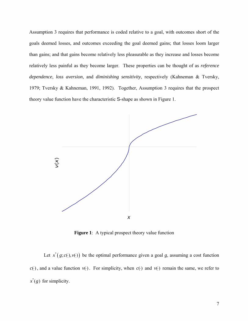
Assumption 3 requires that performance is coded relative to a goal, with outcomes short of the

goals deemed losses, and outcomes exceeding the goal deemed gains; that losses loom larger

than gains; and that gains become relatively less pleasurable as they increase and losses become

relatively less painful as they become larger. These properties can be thought of as reference

dependence, loss aversion, and diminishing sensitivity, respectively (Kahneman & Tversky,

1979; Tversky & Kahneman, 1991, 1992). Together, Assumption 3 requires that the prospect

theory value function have the characteristic S-shape as shown in Figure 1.

x

Figure 1: A typical prospect theory value function

Let ( )* ; ( ), ( )⋅ ⋅x g c v be the optimal performance given a goal g, assuming a cost function

( )⋅c , and a value function ( )⋅v . For simplicity, when ( )⋅c and ( )⋅v remain the same, we refer to

*( )x g for simplicity.

8

Results

Our model predicts that performance will be an inverted U-shaped function of the goal

level: performance increases as goal levels increase for “low” goals and decreases as goal levels

increase for “high” goals. We formalize this statement in the following proposition:

PROPOSITION 1: Let Assumption 1, 2, and 3 hold. Then, (i) *( ) / 0>dx g dg if and only if ( )*( ) 0v x g g′′ − < if and only if *( )x g g> ;

(ii) *( ) / 0<dx g dg if and only if ( )*( ) 0v x g g′′ − > if and only if *( )x g g< .

Proposition 1 indicates that increasing a goal improves absolute performance if

individuals exceed the initial goal (the goal is “easy”), while the opposite is true if individuals do

not exceed the initial goal (the goal is “hard”). As first blush, the second result seems at odds

with previous empirical findings which show that more difficult goals typically increase average

performance. Locke & Latham (1991) report that 91% of 192 studies of goal difficulty have

found that higher goals produce higher performance. Note, however, that Proposition 1 captures

how individual performance changes as a function of different goals, while the studies of goal

difficulty measure how collective performance changes as a result of different goals. Thus,

Proposition 1 is consistent with the goal difficulty result if increased performance by individuals

who are challenged by a higher goal overcomes the decreased performance by individuals who

fall further behind their goal. Heath, Larrick, & Wu (1999, pp. 100-102) show that an

asymmetry of this type occurs under reasonable parametric assumptions—higher goals produce

slightly worse performance for low ability individuals, but dramatically improved performance

for high ability individuals.

9

0 10 20 30 40 50 60 70 80units of performance, x

mar

gina

l cos

t and

be

nefit

func

tions

30( )′b x 40( )′b x

1( )c x′

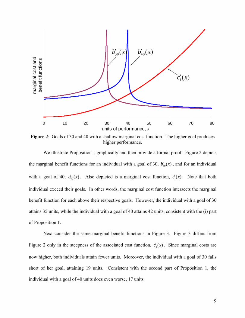
Figure 2: Goals of 30 and 40 with a shallow marginal cost function. The higher goal produces higher performance.

We illustrate Proposition 1 graphically and then provide a formal proof. Figure 2 depicts

the marginal benefit functions for an individual with a goal of 30, 30( )′b x , and for an individual

with a goal of 40, 40( )′b x . Also depicted is a marginal cost function, 1( )′c x . Note that both

individual exceed their goals. In other words, the marginal cost function intersects the marginal

benefit function for each above their respective goals. However, the individual with a goal of 30

attains 35 units, while the individual with a goal of 40 attains 42 units, consistent with the (i) part

of Proposition 1.

Next consider the same marginal benefit functions in Figure 3. Figure 3 differs from

Figure 2 only in the steepness of the associated cost function, 2( )′c x . Since marginal costs are

now higher, both individuals attain fewer units. Moreover, the individual with a goal of 30 falls

short of her goal, attaining 19 units. Consistent with the second part of Proposition 1, the

individual with a goal of 40 units does even worse, 17 units.

10

0 10 20 30 40 50 60 70 80units of performance, x

mar

gina

l cos

t and

be

nefit

func

tions

30( )′b x 40( )′b x

2( )′c x

Figure 3: Goals of 30 and 40 with a steep marginal cost function. The lower goal produces higher performance.

We now prove Proposition 1 formally. To do so, we establish the following Lemma.

LEMMA: Let Assumptions 1, 2, and 3 hold. Then ( ) ( )* *( ) ( )′′ ′′− <v x g g c x g .

PROOF OF LEMMA: Since *( )x g is the optimal performance given goal g,

( ) ( )* *( ) ( )v x g g c x g′ ′− = . By Assumption 1 and 2, * *( ( ) ) ( ( ) ) 0v x g g c x g′ ′− − ε > − ε > for 0ε > .

Therefore, ( ) ( )* *( ) ( )′′ ′′− <v x g g c x g . o

We now use this Lemma to prove Proposition 1.

PROOF OF PROPOSITION 1: Assumption 3 requires that ( )*( ) 0v x g g′′ − < if and only if *( )x g g> ,

and ( )*( ) 0v x g g′′ − > if and only if *( )x g g< . Thus it remains to be proved that *( ) / ( )0dx g dg < > if and only if ( )*( ) ( )0v x g g′′ − > < .

Rewriting Eq. (2) under Assumption 3, we have

(3) ( ) ( )* *( ) ( )c x g v x g g′ ′= − .

Using the implicit function theorem and differentiating Eq. (3) with respect to g, we get:

11

(4) ( ) ( )* *

* *( ) ( )( ) ( ) 1

dx g dx gc x g v x g g

dg dg⎛ ⎞

′′ ′′= − −⎜ ⎟⎝ ⎠

.

Rewriting Eq. (4) yields

(5) ( )

( ) ( )**

* *

( )( )( ) ( )

v x g gdx gdg v x g g c x g

′′ −=

′′ ′′− −.

We use the Lemma to prove the result. By the Lemma, we know that ( ) ( )* *( ) ( ) 0v x g g c x g′′ ′′− − < , which indicates that *( ) /dx g dg and *( ( ) )v x g g′′ − must have

opposite signs. Thus, *( ) / 0dx g dg < if and only if ( )*( ) 0v x g g′′ − > , and *( ) / 0dx g dg > if and

only if ( )*( ) 0v x g g′′ − < . ■

Proposition 1 implies that if an individual surpasses her goal, she could have performed

even better had she increased her goal by a small amount. From Eq. (5) and

( ) ( ) ( )* * *( ) ( ) ( )′′ ′′ ′′− − < −v x g g c x g v x g g , we note that for *( ) >x g g , *( ) 1<dx gdg

. In other

words, increasing a goal by 10 units will increase performance by less than 10 units.

It is also important to note that it is critical that ( )⋅v be strictly concave above the

reference point and strictly convex below it. It is easy to see from Eq. (5) that *( ) 0=

dx gdg

if and

only if ( )⋅v is linear. Thus, a piecewise linear value function with loss aversion will not predict

that higher goals lead to higher performance.

Finally, although it appears that the first and second parts of the Proposition are

inconsistent, they are not. They would be inconsistent for ( )′ ⋅v continuous. However,

Assumption 3 requires that the first derivative of the benefit function be discontinuous.

Proposition 1 requires that the result hold for *( ) 0x g > and for *( )x g g< , because there is a

discontinuity at *( )x g g= .

12

Interpreting effort and persistence

To interpret the empirical results on effort and persistence, we posit two strictly

increasing functions, ( )x h e= and ( )x k t= . The function ( )h ⋅ indicates how many units of

performance is produced by a particular level of effort e, while ( )k ⋅ indicates how many units of

performance is produced by working for a particular time t. We can re-write Eq. (2) as

( ) ( )( ) ( )b h e c h e′ ′= and ( ) ( )( ) ( )b k t c k t′ ′= respectively and solve for the optimal e and t. The

results will be identical since ( )h ⋅ and ( )k ⋅ are strictly increasing. To see the required result, let

*( )e g be the optimal effort for a goal g. The First Order Condition is now obtained by

differentiating the following equation with respect to *( )e g :

( )( ) ( ) ( )( ) ( )* * * *( ) ( ) ( ) ( )c h e g h e g v h e g g h e g′ ′ ′ ′= − .

After implicitly differentiating with respect to g and re-arranging, this becomes

( )( ) ( )

( )( ) ( ) ( )( ) ( )* **

* * * *

( ) ( )( )( ) ( ) ( ) ( )

v h e g g h e gde gdg v h e g g h e g c h e g h e g

′′ ′−=

′′ ′ ′′ ′− −.

Since ( )*( )h e g′ can be factored out of the numerator and denominator and, by assumption,

*( ) /de g dg is always the same sign as *( ) /dx g dg , the results of Proposition 1 follow

immediately. The analysis for persistence is identical and hence is omitted.

3. Goals and Attention

We noted above that goals direct attention from one activity to another. Studies have

shown that individuals given a goal on, say, quantity, improve quantity but not other

performance dimensions, such as quality. We show that this result also follows from a prospect

theory model of goal behavior.

13

Let there be n dimensions of performance. For simplicity, we let the first dimension

denote the dimension with the goal intervention. We denote the performance on dimension i, ix .

As before, we assume that an individual has a utility function that is additively separable in costs

and benefits. Moreover, we assume that the benefit function is additively separable in the uni-

dimensional benefit functions. In particular, the utility function U(x) has the following form,

(6) 1

( ) ( ) ( )=

= −∑n

i i i i ii

U x wv x c x

where ( )i iv x and ( )i ic x are the value and cost of attaining 0≥ix units and iw is the weight for

dimension i.

We assume that performance, 1( ,..., )nx x , is a function of time allocated to each

dimension, i.e., ( )=i i ix f t . We let it denote the time devoted to dimension i and impose the

constraint that 1=

≤∑n

ii

t T , the total amount of time available. We assume that there are positive

returns to an additional unit of time devoted to dimension i.

Assumption 4 (Positive returns on time): For all i, ( ) 0′ >if t .

We also make an assumption about the cost function that is analogous to Assumption 2, cost is

an increasing function of the time expended on a particular dimension:

Assumption 5 (Cost function): The cost function has the following properties: for all i, ( ) 0ic ⋅ > and ( ) 0′ ⋅ >ic .

We next consider the form of the value function. Recall that the first dimension is the

one with the goal intervention.

Assumption 6 (Value function): The value function has the following properties:

(i) 1( )⋅v has the properties of ( )⋅v in Assumption 3;

14

(ii) for all 1>i , ( ) 0, ( ) 0i iv x v x′ ′′> < .

Assumption 6 requires that the value function for the first dimension is defined with respect to a

goal g and inherits the properties of the prospect theory value function. The value functions for

all other dimensions are concave and increasing.

Finally, we assume that individuals maximize (6) by choosing the best allocation of time,

* *1( ,..., )nt t , i.e., the maximization problem is equivalent to:

(7) ( ) ( ) ( )1,..., 1 1 1 1 1

2 1

Max ( ,..., ) ( ) ( ) ( ) .= =

= − + −∑ ∑n

n n

t t n i i i i i i ii i

U x x w v f t g wv f t c f t

We prove the following Proposition that relates goals to attention:

PROPOSITION 2: Let Assumptions 1 and 4 through 6 hold. Then (i) if * *

1 1 1( )= >x f t g then *1 ( ) / 0>dt g dg ;

(ii) if * *1 1 1( )= <x f t g then *

1 ( ) / 0<dt g dg .

PROOF OF PROPOSITION 2: The first order condition is

(8) ( ) ( ) ( ) ( )* * * * * *1 1 1 1 1 1 1 1( ) ( ) ( ) ( )j j j j j j j jw v f t g f t c t w v f t f t c t′ ′ ′ ′ ′ ′− − = − = λ ,

for all 1,...,j n= , where λ is the Lagrange multiplier for the constraint on time. If *

1=

=∑n

ii

t T ,

then 0λ ≥ , otherwise 0λ = . Using the implicit function theorem and differentiating Eq. (8) with respect to g, we get:

(9) ( )( ) ( )( )* *

* *1 11 1 1 1 1 1 1

( ) ( )( ) ( ) 1

⎛ ⎞′′ ′′= − −⎜ ⎟

⎝ ⎠

dt g dt gc f t g w v f t g g

dg dg.

Rewriting Eq. (9), we get ( )( )

( )( ) ( )( )**

1 1 1 11* *

1 1 1 1 1 1 1

( )( )( ) ( )

w v f t g gdt gdg w v f t g g c f t g

′′ −=

′′ ′′− −. The rest of the proof

follows by applying the logic used in the proof of Proposition 1. ■

We might expect a change in the goal on the targeted dimension to affect performance on

the other dimensions, when the time constraint is binding, *

1=

=∑n

ii

t T . Indeed, this is the case.

15

The following Proposition establishes that in the presence of a time constraint, increasing the

goal on one dimension results in lower performance on another dimension.

PROPOSITION 3: Let Assumptions 1 and 4 through 6 hold. Then for 1≠j , if * *1 1 1( )= >x f t g , then

*( ) / 0≤jdt g dg .

PROOF OF PROPOSITION 3: Implicitly differentiating (8) with respect to g for 1=j and 1≠j , we get:

(10) ( ) ( )( )* *

* *1 11 1 1 1 1 1 1

( ) ( )( ( ) ) 1 ( )

⎛ ⎞′′ ′′− − − =⎜ ⎟

⎝ ⎠

dt g dt gw v f t g g c f t g

dg dg

( )( ) ( )( )* *

* *( ) ( )( ) ( )′′ ′′−j j

j j j j j j j

dt g dt gw v f t g c f t g

dg dg.

If * *1 1 1( )= >x f t g , then from Proposition 2, we know that *

1 ( ) / 0>dt g dg , and, from above, that *1 ( ) 1<dt gdg

. Therefore, it is clear that the left-hand side of Eq. (10) is negative. Since

( )( ) ( )( )* *( ) ( ) 0j j j j j j jw v f t g c f t g′′ ′′− = λ ≥ , *( ) / 0≤jdt g dg . ■

4. Piling Up

In this section, we show that a new implication called “piling up” follows from certain

reasonable assumptions concerning the value function, in particular, assumptions about loss

aversion. Informally, piling up implies that performance for “moderately” challenging goals will

tend to exceed the goal, but only by a very little. In other words, performance will tend to “pile

up” around the goal.

To illustrate, consider low, medium, and high ability producers, who must exert high,

medium, and low cost respectively to produce the same number of units of performance (see

Figure 4). Next, consider a goal of 10 units. This goal is “easy” in the sense that the low,

medium, and high ability producers all exceed the goal by a generous margin, completing 21, 26,

and 33 units respectively.

16

We now consider the “medium” goal of 35 units depicted in Figure 5. The goal of 35

units is more challenging – all three of our individuals exceed the goal, but never by much. Our

high ability producer completes 41 units, exceeding the goal by 6 units, whereas the medium and

low ability producers complete 36 and 35 units respectively.

Finally, we turn to a “high” goal of 60 units (Figure 6). This goal is sufficiently

challenging that only the high ability producer completes the goal, achieving 61 units. The

medium and low ability producers achieve 32 and 24 units respectively.

In this demonstration, low and high goals yield the highest variation in performance,

whereas the medium goal has the lowest spread. In addition, note that the medium goal induces

performance that exceeds the goal of 35 units by a small amount. In other words, performance

“piles up” around the goal. Note also that this numerical example is consistent with the goal

difficulty effect: the highest goal of 60 units leads to the highest average performance, even

though two of the three producers fall short of the goal. The goal setting literature generally

reports means but not distributions of performance. One exception is Garland (1985), who found

that the variance for an extremely challenging goal was 75% higher than the variance for a

somewhat less challenging goal (see Heath, Larrick, & Wu, 1999, pp. 101-102).

We tie the intuitive notion of piling up to the value function and show how piling up is

related to loss aversion. First, we formalize the notion of piling up. The definition defines a set

of goals in which performance exceeds a particular goal by δ or less.

DEFINITION: For a particular cost function, ( )⋅c , and a particular value function, ( )⋅v , a set of goals, ( ); ( ), ( )δ ⋅ ⋅G c v , exhibits δ-piling up if for all

( ); ( ), ( )g G c v∈ δ ⋅ ⋅ , ( )*0 ; ( ), ( )≤ ⋅ ⋅ − ≤ δx g c v g .

To show that “piling up” is an implication of loss aversion, we first make a simplifying

assumption about loss aversion that follows Tversky & Kahneman (1991).

17

Assumption 7 (Constant Loss Aversion): The value function, ( )⋅v , exhibits constant loss aversion, i.e., for all 0>x , ( ) ( )− − =v x kv x .

0 10 20 30 40 50 60 70 80units of performance, x

mar

gina

l cos

t and

ben

efit

func

tions ′c xL( )

′c xM ( )′c xH ( )10 ( )′b x

Figure 4: An easy goal with low, medium, and high ability producers

0 10 20 30 40 50 60 70 80units of performance, x

mar

gina

l cos

t and

ben

efit

func

tions ′c xL( )

′c xM ( )′c xH ( )

35 ( )b x′

Figure 5: A medium goal with low, medium, and high ability producers

18

We prove the following Proposition on piling up.

PROPOSITION 4: Let Assumption 1, 2, and 3 hold. Also, let Assumption 7 hold for 1( )⋅v and

2( )⋅v . Finally, let 1 2( ) ( )=v x v x for 0>x , 1 1 1( ) ( )− − =v x k v x and 2 2 2( ) ( )− − =v x k v x for 0<x , where 1 2<k k . Then, for all δ , ( ) ( )1 2; ( ), ( ) ; ( ), ( )G c v G c vδ ⋅ ⋅ ⊆ δ ⋅ ⋅ .

We interpret Proposition 4 as requiring that the set of goals that satisfy δ-piling up

weakly increases as the loss aversion coefficient increases, all else equal. Proposition 4 assumes

that individuals have the same marginal cost function, ( )⋅c , the same value function, but may

differ on individual goals. As the loss aversion coefficient increases, the number of individuals

who exceed their goal by a small amount increases as well.

0 10 20 30 40 50 60 70 80units of performance, x

mar

gina

l cos

t and

ben

efit

func

tions ′c xL( )′c xM ( )′c xH ( )

60 ( )b x′

Figure 6: A high goal with low, medium, and high ability producers

PROOF OF PROPOSITION 4: We prove the result by contradiction. Assume that Proposition 4 is false. Then there exists some g′ , such that ( )1; ( ), ( )g G c v′∈ δ ⋅ ⋅ but ( )2; ( ), ( )g G c v′∉ δ ⋅ ⋅ . If

( )2; ( ), ( )g G c v′∉ δ ⋅ ⋅ , then either ( )*2; ( ), ( )x g c v g′ ′⋅ ⋅ − > δ or ( )*

2; ( ), ( ) 0x g c v g′ ′⋅ ⋅ − < . Consider

the first case. By Assumption 1, ( )( ) ( )( )* *2 2 2 2; ( ), ( ) ; ( ), ( )v x g c v g c x g c v g′ ′ ′ ′ ′ ′⋅ ⋅ − = ⋅ ⋅ − , but

19

( ) ( )2 2′ ′>v x c x for all ( )*2; ( ), ( )x x g c v′< ⋅ ⋅ . However, ( )( )*

2 1; ( ), ( )v x g c v g′ ′ ′⋅ ⋅ − =

( )( )*2 1; ( ), ( )c x g c v g′ ′ ′⋅ ⋅ − since and 2( )v ⋅ coincide in the gains. Thus, ( )*

2; ( ), ( ) 0x g c v g′ ′⋅ ⋅ − < < δ .

In this case, Assumption 1 implies that there exists x g′< such that ( ) ( )2 2v x c x′ ′= . However,

since 1 2k k< , ( ) ( )1 2v x c x′ ′< , which implies that ( )*1; ( ), ( )x g c v g′ ′⋅ ⋅ < which is a contradiction. ■

An alternative formulation of piling up is found below. This proposition begins with a

different premise. We assume that Individuals 1 and 2 have the same value function but

different cost functions, 1( )c ⋅ and 2( )c ⋅ . Proposition 5 requires that there exists a sufficiently

large loss aversion coefficient that if Individual 1 surpasses the goal by a small amount, then

Individual 2 with a steeper cost function will also surpass the goal.

PROPOSITION 5: Let Assumption 1 hold, Assumption 2 hold for 1( )c ⋅ and 2( )c ⋅ , and Assumptions 3 and 7 hold for 1( )v ⋅ and 2( )v ⋅ , where 1 1 1( ) ( )v x k v x− − = for 0x < , 1 2( ) ( )v x v x= for 0x > , and

2 2 2( ) ( )v x k v x− − = for 0x < , where 1 2k k< . Also, let ( )2 1( ) ( )c x f c x= for ( )f ⋅ strictly

increasing and 2( )c ⋅ be bounded above for all ( )1 1; ( ), ( )g G c v∈ δ ⋅ ⋅ . Then there exists a finite 2k

such that if ( )1 1; ( ), ( ) ,g G c v∈ δ ⋅ ⋅ then ( )2 2; ( ), ( ) .g G c v∈ δ ⋅ ⋅

PROOF OF PROPOSITION 5: If ( )2 1; ( ), ( )g G c v∈ δ ⋅ ⋅ , then the Proposition clearly holds. Thus, we

must consider the case in which ( )1 1; ( ), ( )g G c v∈ δ ⋅ ⋅ and ( )2 1; ( ), ( )g G c v∉ δ ⋅ ⋅ . The latter implies

that for some 1 0x < , ( ) ( )1 1 2 1v x c x′ ′= . Thus, if 1 2k k< , ( ) ( )2 1 2 1v x c x′ ′> . The 2k that establishes

Proposition 5 can be constructed similarly: ( )( )

220

1 1

max x

c xkk v x<

′= + ε

′ for some arbitrarily small ε .

Such a 2k can always be found and is finite since 2( )c ⋅ is bounded above. ■

5. Subgoals and the Starting Problem

The “goals as reference points” approach suggests that individuals far away from the goal

may give up because they do not feel that they are making sufficient progress toward the goal.

Heath, Larrick & Wu (1999) called this the “starting problem” and presented some empirical

evidence supporting this implication.

20

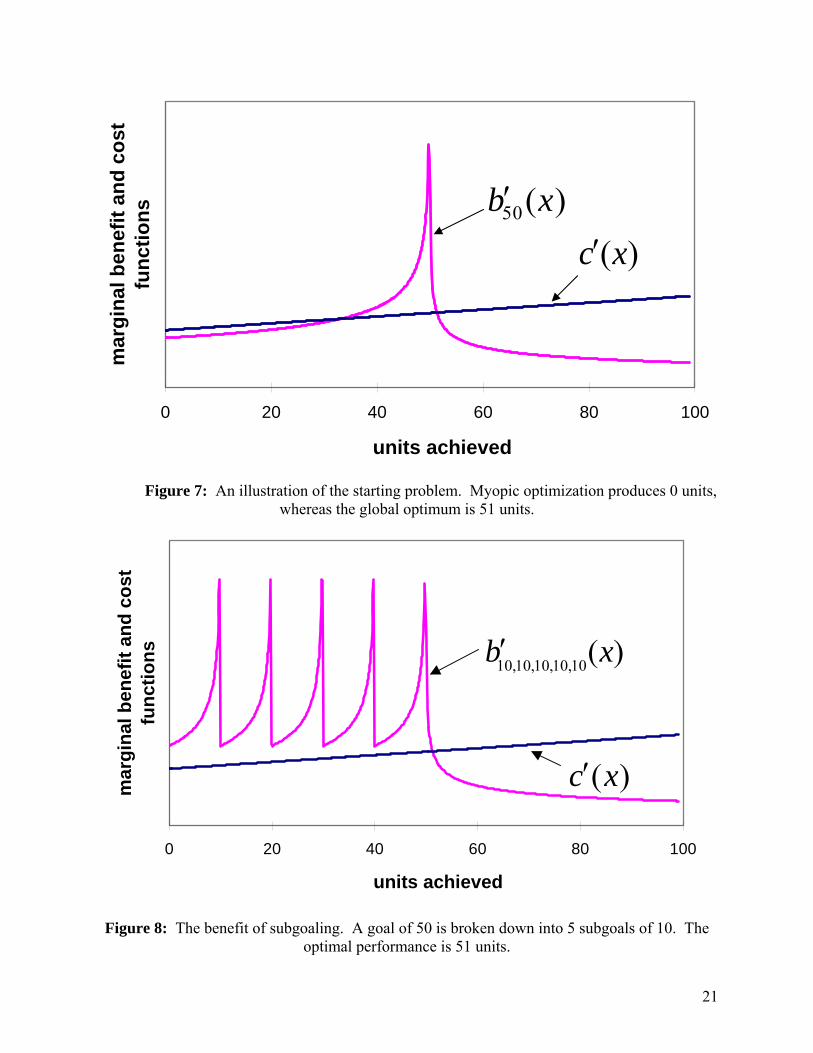
The starting problem is relevant when forward looking and myopic optimization produce

different levels of performance. Figure 7 illustrates such a situation. Since ( )0 (0)c v′ ′> , under

myopic optimization, this individual stops immediately. Note, however, that ( )′c x is quite flat,

and ( ) ( )c x v x g′ ′< − for 35>x . Indeed, the global optimum is * 51x = .

More formally, the starting problem follows from diminishing sensitivity of the value

function in losses. Since ( )v x g′ − might be close to zero for large g, it is possible that

( ) ( )c x v x g′ ′> − for small x. The starting problem depicted in Figure 7 can be overcome if the

goal of 50 is broken down into subgoals. For example, suppose that an individual sets five

subgoals of 10. Now, the individual is never more than 10 units away from the goal. This

transformation is illustrated in Figure 8. The saw-toothed marginal benefit function is written

10,10,10,10,10 ( )′b x to indicate the division of the goal of 50 into 5 subgoals of 10. The optimal

performance under subgoaling is * 51x = , even in the case of myopic optimization.

More generally, suppose that a goal g is decomposed into n subgoals of sg such that

sg ng= . The subgoals serve to redefine the marginal benefit function:

,...,

( ), ( 1)( )

( ),s s

s s sg g

v x ig i g x igb x

v x g x g′ − − < <⎧′ = ⎨ ′ − >⎩

,

where 1,...,i n= indexes the subgoals. It is easy to see that subgoaling cannot decrease

performance and may help. To see this, it is sufficient to note that ,..., ( ) ( )s sg g gb x b x′ ′≥ for all x.

Of course, the two functions coincide for x g> . For x g< , ( ) ( )sv x ig v x g′ ′− ≥ − for all 1i ≥

since sx ig x g− ≤ − for 1,...,i n= and ( ) 0v x′′ > for 0x < .

21

0 20 40 60 80 100

units achieved

mar

gina

l ben

efit

and

cost

fu

nctio

ns 50( )b x′

( )c x′

Figure 7: An illustration of the starting problem. Myopic optimization produces 0 units,

whereas the global optimum is 51 units.

0 20 40 60 80 100

units achieved

mar

gina

l ben

efit

and

cost

fu

nctio

ns

( )c x′

10,10,10,10,10( )b x′

Figure 8: The benefit of subgoaling. A goal of 50 is broken down into 5 subgoals of 10. The optimal performance is 51 units.

22

6. General Discussion

We proposed a very simple model to explain the stylized findings in the goal setting

literature. The model adopts the “goals as reference points” approach developed in Heath,

Larrick, & Wu (1999) to explain how higher goals lead to higher performance. We also explain

how effort, persistence, and attention can be interpreted as mechanisms within this framework.

The framework also generates some new predictions, such as the tendency of performance to

“pile up” around moderately challenging goals and the performance benefits of subgoals.

By systematically explaining three major classes of empirical results, our model adds to

previous approaches in the literature which have implicitly or explicitly used particular

assumptions about the shape of the value function to explain an occasional result. For example,

a linear value function was used by Locke & Latham (1991, p. 222) to explain why goals affect

satisfaction, but Proposition 1 shows that diminishing sensitivity is necessary to explain how

higher goals increase performance. Moreover several researchers have implicitly or explicitly

proposed step-function value functions to explain various aspects of goal-setting phenomena

(e.g., Simon, 1955; Campion & Lord, 1982). Such functions do not exhibit diminishing

sensitivity and hence have the same problem as linear value functions. What we find exciting

about this approach is that the value function, which has received robust support in many other

areas of research, contains properties that seem essential for explaining the empirical results of

the goal-setting literature—not only diminishing sensitivity in Proposition 1, but also loss

aversion in Propositions 4 and 5. By proposing a way to link the value function with the goal

setting literature, we provide a way of unifying two large empirical literatures with a single

underlying theoretical approach.

23

We see two main advantages of this modeling approach: parsimony and precision. Other

attempts to explain the stylized findings in the goal setting literature have evoked at least three

mechanisms: effort, persistence, and attention. Our model offers a more parsimonious story,

subsuming all three of these mechanisms. The model also has the benefit of precision. Although

it is simple in structure, it is nonetheless powerful enough to make new behavioral predictions as

illustrated by the results on piling up and subgoaling.

We close by suggesting some directions for extending our model. Other researchers have

tried to explain goal setting results in terms of expectancies: higher goals lead to higher

expectancies, and hence increased performance. Although we believe that expectancies play a

role in goal setting, in keeping with our emphasis on parsimony and precision, we have not

added an expectancy component to our current model. An expectancy story would be more

complex and is not needed to explain the goal setting literature’s major findings. Furthermore,

we currently lack a precise model to link expectations and behavior. However, we suspect that

there are other goal-setting phenomena that are not well-explained by a value function account,

and future research might investigate the implications of an expectancy-based model akin to our

value function-based model.

Another direction to extend the current work would be to consider endogenous goals.

For the most part, the goal setting literature has considered externally-determined goals even

though we know that individuals use goals to regulate their own behavior, whether they are

studying, exercising, or performing thankless chores. Endogenous goal setting is a topic that

deserves more attention and might be modeled by extending our framework to include a

principal-agent setup (e.g., Grossman & Hart, 1983), akin to the planner-do models used by

Thaler & Shefrin (1981). The planner would declare a goal, and the doer would respond

24

optimally to that goal using the framework developed here. This setup might be complicated by

the planner’s imperfect understanding of the doer’s “type” (the doer might be a low ability or

high ability type), and thus the planner and doer can be seen as playing a game of incomplete

information (Harsanyi, 1967-68).

Applications of prospect theory to economics, finance, law, medicine, and public policy

have yielded important insights (e.g., Barberis, Huang, & Santos, 2001; Bowman, Minehart, &

Rabin, 1997), but most of these have used the status quo as a reference point. Recently,

however, there is a growing body of literature that has investigated non-status quo reference

points (e.g., Camerer et al., 1997; Goette, Huffman, & Fehr, 2004; Hardie, Fader, & Johnson,

1993; Heath, Huddart, & Lang, 1999). For example, Camerer et al. showed evidence for income

targeting for New York City cab drivers. Many cab drivers appear to set daily earnings targets

(i.e., an income goal), going home when they exceed their daily goal. This seemingly plausible

behavior creates a paradox: drivers exceed their goal more rapidly on favorable days (e.g., a

rainy day with lots of conventions in town), so they end up working fewer hours on “high wage”

days and more hours on “low wage” days — a violation of standard labor theory. By

understanding more precisely the influence of goals on behavior, we will be in a better position

to understand a number of important organizational and economic phenomena.

25

References

Bandura, A., & Cervone, D. (1983). “Self-evaluative and self-efficacy mechanisms

governing the motivational effects of goal systems.” Journal of Personality and Social

Psychology, 45, 1017-1028.

Bandura, A. & Schunk, D.H. (1981). “Cultivating competence, self-efficacy, and

intrinsic interest through proximal self-motivation.” Journal of Personality and Social

Psychology, 41, 586-98.

Barberis, N., Huang, M., & Santos, T. (2001). “Prospect Theory and Asset Prices.”

Quarterly Journal of Economics, 116, 1-53.

Bavelas, J. & Lee, E. (1978). “Effects of goal level on performance: A trade-off of

quantity and quality.” Canadian Journal of Psychology, 32, 219-239.

Botterill, C.B. (1977). “Goal setting and performance on an endurance task.” University

of Alberta, unpublished doctoral dissertation.

Bowman, D., Minehart, D., & Rabin, M. (1999). “Loss aversion in a consumption-

savings model.” Journal of Economic Behavior and Organization, 38, 155-178.

Bryan, J.F., & Locke, E.A. (1967). “Parkinson's law as a goal-setting phenomenon.”

Organizational Behavior and Human Performance, 2, 258-275.

Camerer, C., Babcock, L., Loewenstein, G., & Thaler, R. (1997). “Labor supply of New

York City cabdrivers: One day at a time.” Quarterly Journal of Economics, 112, 407-441.

Campion, M.A., & Lord, R.G. (1982). “A control systems conceptualization of the goal-

setting and changing process.” Organizational Behavior and Human Performance, 30, 265-287.

Garland, H. (1982). “Goal levels and task performance: A compelling replication of

some compelling results.” Journal of Applied Psychology, 67, 245-48.

26

Garland, H. (1985). “A cognitive mediation theory of task goals and human

performance.” Motivation and Emotion, 9, 345–367.

Goette, L., Huffman, D., & Fehr, E. (2004). Loss Aversion and Labor Supply. Journal of

the European Economic Association, 2, 216-228.

Grossman, S.J. & Hart, O.D. (1983). “An Analysis of the Principal-Agent Problem.”

Econometrica, 51, 7-46.

Hall, H.K., Weinberg, R.S., & Jackson, A. (1987). “Effects of goal specificity, goal

difficulty, and information feedback on endurance performance.” Journal of Sport Psychology,

9, 43-54.

Hardie, B.G.S., Johnson, E.J., & Fader, P.S. (1993). “Modeling Loss Aversion and

Reference Dependence Effects on Brand Choice.” Marketing Science, 12, 378-394.

Harsanyi, J.C. (1967). “Games with Incomplete Information Played by Bayesian Players,

I-III.” Management Science 14, 159-182, 320-334, 486-503.

Heath, C., Huddart, S., & Lang, M. (1999). “Psychological factors and stock option

exercise.” Quarterly Journal of Economics, 114, 601-627.

Heath, C., Larrick, R.P., & Wu, G. (1999). “Goals as reference points.” Cognitive

Psychology 38, 79-109.

Huber, V.L. & Neale, M.A. (1987). “Effects of self-and competitor goals on

performance in an interdependent bargaining task.” Journal of Applied Psychology, 72, 197-203.

Kahneman, D., & Tversky, A. (1979). “Prospect theory: An analysis of decision under

risk.” Econometrica, 47, 263-291.

LaPorte, R.E., & Nath, R. (1976). “Role of performance goals in prose learning.”

Journal of Educational Psychology, 68, 260-264.

27

Latham, G. P., & Locke, E.A. (1975). “Increasing productivity with decreasing time

limits: A field replication of Parkinson’s law.” Journal of Applied Psychology, 60, 524-526.

Locke, E.A. (1982). “Relation of goal level to performance with a short work period and

multiple goal levels.” Journal of Applied Psychology, 67, 512-514.

Locke, E.A., & Bryan, J.F. (1969). “The directing function of goals in task

performance.” Organizational Behavior and Human Performance, 4, 35-42.

Locke, E.A., Cartledge, N., & Knerr, C. (1970). “Studies of the relationship between

satisfaction, goal-setting and performance.” Organizational Behavior and Human Decision

Processes, 5, 135-58.

Locke, E.A. & Latham, G.P. (1990). A theory of goal setting and task performance.

Englewood Cliffs, NJ: Prentice-Hall.

Locke, E.A. & Latham, G. (1991). “Self-regulation through goal setting.”

Organizational Behavior and Human Decision Processes, 50, 212-247.

Mento, A.J., Steel, R.P., & Karren, R.J. (1987). “A meta-analytic study of the effects of

goal setting on task performance: 1966-1984.” Organizational Behavior and Human Decision

Processes, 39, 52-83.

Naylor, J.C., & Ilgen, D.R. (1984). “Goal setting: A theoretical analysis of a

motivational technology.” In L.Cummings & B. Staw (Eds.), Research in Organizational

Behavior (pp. 95-140). Greenwich, CT: JAI Press.

Neale, M.A., & Bazerman, M.H. (1985). “The effect of externally set goals on reaching

integrative agreements in competitive markets.” Journal of Occupational Behavior, 6, 19-32.

28

Nemeroff, W.F., & Cosentino, J. (1979). “Utilizing feedback and goal setting to increase

performance appraisal interviewer skills of managers.” Academy of Management Journal, 22,

566-576.

Ness, R.G., & Patton, R.W. (1979). “The effect of beliefs on maximum weight-lifting

performance.” Cognitive Therapy and Research, 3, 205-211.

Organ, D.W. (1977). “Intentional vs. arousal effects of goal setting.” Organizational

Behavior and Human Performance, 18, 378-389.

Roberts, G.C., & Hall, H.K. (1987). “Motivation in sport: Goal setting and

performance.” Department of Kinesiology, University of Illinois, unpublished manuscript (cited

in Locke & Latham, 1990).

Rothkopf, E.Z., & Billington, M.J. (1979). “Goal-guided learning from text: Inferring a

descriptive processing model from inspection times and eye movements.” Journal of

Educational Psychology, 71, 310-327.

Sales, S.M. (1970). “Some effects on role overload and role underload.” Organizational

Behavior and Human Performance, 5, 592-608.

Siegel, S., & Fouraker, L.E. (1960). Bargaining and group decision making. New York:

McGraw-Hill.

Simon, H.A. (1955). “A behavioral model of rational choice.” Quarterly Journal of

Economics, 69, 99-118.

Singer, R.N., Korienek, G., Jarvis, D., McColskey, D., & Candeletti, G. (1981). “Goal

setting and task persistence.” Perceptual and Motor Skills, 53, 881-882.

Stevenson, M.K., Kanfer, F.H., & Higgins, J.M. (1984). “Effects of goal specificity and

time cues on pain tolerance.” Cognitive Therapy and Research, 8, 415-426.

29

Thaler, R.H., & Shefrin, H.M. (1981). “An economic theory of self-control.” Journal of

Political Economy, 89, 392-410.

Tversky, A., & Kahneman, D. (1991). “Loss aversion in riskless choice: A reference-

dependent model.” Quarterly Journal of Economics, 106, 1039-1061.

Tversky, A., & Kahneman, D. (1992). “Advances in prospect theory: Cumulative

representations of uncertainty.” Journal of Risk and Uncertainty, 5, 297-323.

Wyer, R.S., Srull, T.K., Gordon, S.E., & Hartwick, J. (1982). “Effect of processing

objectives on the recall of prose material.” Journal of Personality and Social Psychology, 43,

674-688.